Temporal-Difference estimation of dynamic discrete choice models

Abstract.

We study the use of Temporal-Difference learning for estimating the structural parameters in dynamic discrete choice models. Our algorithms are based on the conditional choice probability approach but use functional approximations to estimate various terms in the pseudo-likelihood function. We suggest two approaches: The first -linear semi-gradient- provides approximations to the recursive terms using basis functions. The second -Approximate Value Iteration- builds a sequence of approximations to the recursive terms by solving non-parametric estimation problems. Our approaches are fast and naturally allow for continuous and/or high-dimensional state spaces. Furthermore, they do not require specification of transition densities. In dynamic games, they avoid integrating over other players’ actions, further heightening the computational advantage. Our proposals can be paired with popular existing methods such as pseudo-maximum-likelihood, and we propose locally robust corrections for the latter to achieve parametric rates of convergence. Monte Carlo simulations confirm the properties of our algorithms in practice.

1. Introduction

Recent years have seen a number of important developments in the field of Reinforcement Learning (RL) for computation of value functions. The goal of this paper is to study the use of a popular RL technique, Temporal-Difference (TD) learning, for estimation and inference in Dynamic Discrete Choice (DDC) models.

DDC models are frequently used to describe the inter-temporal choices of forward-looking individuals in a variety of contexts. In these models, agents maximize their expected future payoff through repeated choice amongst a set of discrete alternatives. Based on a revealed preference argument, structural estimation proceeds by using microdata on choices and outcomes to recover the underlying model parameters. A key challenge in this literature is the complexity of estimation. Uncovering the structural parameters originally required an explicit solution to a dynamic programming problem in addition to the optimization of an estimation criterion. A key advance has been Hotz and Miller’s (1993) Conditional Choice Probability (CCP) algorithm which avoids the repeated solution of the inter-temporal optimization problem by taking advantage of a mapping between value function differences and conditional choice probabilities.

Unfortunately, the standard CCP algorithm is computationally infeasible when the underlying states are continuous and/or the state space is high-dimensional. Such state spaces are common in applications. One frequently employed approach to tackle continuous state spaces is through state space discretization, e.g., Kalouptsidi (2014) and Almagro and Domınguez-Iino (2019) use aggregation and clustering methods to do this. However, it is not always clear how to perform such a discretization in practice, and moreover, it introduces bias into the parameter estimates. An alternative is to employ functional approximations for the value functions. For instance, Barwick and Pathak (2015) and Kalouptsidi (2018) use estimated transition densities and numerical/analytical integration to approximate the value functions using linear sieves and LASSO, respectively. However, the theoretical properties of these methods when using machine learning methods (such as LASSO) are as yet unknown, and they still require estimation of transition densities, which is not straightforward, along with numerical integration, which can be computationally expensive.

The aim of this paper is to develop tractable algorithms for CCP estimation when the state variables are continuous and/or the state space is large. Such algorithms should possess three properties: First, they should be fast to compute even under high-dimensional state spaces. Second, they should avoid state space discretization, and instead rely on functional approximation of value functions. Third, they should avoid estimation of transition densities which are difficult to parameterize and estimate under continuous states.

In this paper, we suggest two methods, based on the idea of TD learning, that satisfy all the above properties. The methods involve two different techniques for estimating various recursive terms (which are akin to value functions) that arise in CCP estimation. The first approach, the linear semi-gradient method, provides functional approximations to the recursive terms using basis functions. This approach simply involves inverting a low-dimensional matrix, where the dimension is the number of basis functions being used. Thus the computational cost is trivial in most settings. Furthermore, it only requires the observed sequences of current and future state-action pairs as input and estimation of transition densities is not needed. The second approach, Approximate Value Iteration (AVI), builds a sequence of approximations to the value terms by solving a non-parametric estimation problem in each step. Almost any machine learning (ML) method devised for prediction can be used for approximation under this method, including (but not limited to) LASSO, random forests and neural networks. To the best of our knowledge, the AVI estimator is the first estimator for DDC models that can be applied with any ML method. Hence, it naturally allows for very high-dimensional state spaces. Again, no estimation of transition densities is required. We derive the non-parametric rates of convergence for estimation of the value terms under both these methods. With the estimates of these functions at hand, estimation of the structural parameters can proceed with standard methods such as pseudo-maximum-likelihood estimation (PMLE, Aguirregabiria and Mira (2002)) or minimum distance estimation.

The focus of this paper is on the estimation of structural parameters. To this end, our procedures allow one to avoid modeling state transitions. Performing counterfactual analysis may still require estimating the transition density, but we argue that our techniques remain useful, even for this purpose, for two reasons: First, counterfactuals often involve new transition densities which are different from the ones that enter the estimation of the structural parameters, see Kalouptsidi (2018) for an example. Our methods therefore avoid estimation of the original transition densities that may not be needed for counterfactual analysis. Second, with continuous states, decoupling the estimation of structural parameters and transition densities may be beneficial for robustness and efficiency reasons. For instance, it is common to employ AR (e.g., Aguirregabiria and Mira, 2007; Kalouptsidi, 2014) or VAR (Barwick and Pathak, 2015) specifications for transition densities. However, even within these specifications there are a number of choices to be made (e.g., dimension of VARs, distribution of error terms etc) and the estimates of the structural parameters may not be robust to these choices. More importantly, even when non-parametric estimates of transition densities are available, simply plugging them into the second-stage PMLE criterion would seriously degrade the rate of convergence of structural parameters. One would need to adjust the PMLE to account for the non-parametric first stage, but it is not known what form this adjustment takes. By contrast, our proposals employ non-parametric estimates of value functions, and as described below, we derive the necessary adjustments to account for this. To carry out counterfactual analysis, we therefore suggest plugging in our estimates of the structural parameters, which do not rely on non-parametric estimates of transition densities and are robust to mis-specification, together with non-parametric estimates of the transition densities.

The above discussion highlights that in continuous state spaces, estimation of structural parameters is inherently a problem of semi-parametric estimation. In fact, even under discrete states, Aguirregabiria and Mira (2002) show that estimation of transition densities affects the variance of the structural parameter estimates. If the state variables are continuous, existing two-step CCP methods, such as the PMLE will no longer converge at parametric rates. We therefore derive a locally robust estimator by adding a correction term to the PMLE criterion function that accounts for the non-parametric estimation of value function terms using either of our TD methods. We emphasize that this construction is novel and does not directly follow from existing results, e.g., in Chernozhukov et al. (2022). Its computation is particularly straightforward under the linear semi-gradient approach. The resulting estimator converges at parametric rates under continuous states and unrestricted transition densities.

Our TD estimators are thus consistent, computationally very cheap, and they converge at parametric rates. Importantly, they provide a feasible estimation method when the states are continuous and/or the state space is large. This is particularly important for the estimation of dynamic discrete games. Even with discrete states, existing methods for the estimation of dynamic games (Bajari et al., 2007; Aguirregabiria and Mira, 2007; Pesendorfer and Schmidt-Dengler, 2008) require integrating out other players’ actions. With many players, or under continuous states, this can get quite cumbersome. By contrast, our procedure works directly with the joint empirical distribution of the states and their sample successors. Thus the ‘integrating out’ is done implicitly within the sample expectations.

Finally, we also incorporate permanent unobserved heterogeneity into our methods by combining the TD estimation with an Expectation-Maximization (EM) algorithm (Dempster et al., 1977).

A range of Monte Carlo studies confirm the workings of our algorithms. First, we present simulations based on the dynamic firm entry problem described in Aguirregabiria and Magesan (2018). The model has seven structural parameters of interest and five continuous state variables. Existing methods usually struggle at this dimensionality; certainly, discretization of the state space would not work too well. We show simulations using both the linear semi-gradient method and the AVI method where we estimate the value function terms using random forests, and derive results both with and without locally robust correction. Our findings suggest that while the linear semi-gradient has very little bias even without the locally robust correction, the AVI method has slightly higher small sample bias which is substantially reduced when using our locally robust estimator. Overall, our estimators perform very well in this setting and they outperform CCP estimators that employ discretization, leading to a 4 to 11-fold reduction in average mean squared error across the seven structural parameters of interest.

Second, we test our algorithms for dynamic discrete games based on a firm entry game similar to that outlined in Aguirregabiria and Mira (2007). We use the linear semi-gradient method here and, as before, our estimates are closely centered around the true parameters. Since this approach requires the selection of a set of basis functions for the functional approximations, we present results for different sets of basis functions (a second, third and fourth order polynomial) in this model. Our findings suggest that the choice of basis functions has only a small effect on the performance of the estimator. Moreover, we show that a simple cross-validation procedure may be used to select the preferred set of functions.

1.1. Related literature

The paper contributes to the literature on estimation of DDC models. Rust (1987) is the seminal work in this literature. Motivated by computational considerations, Hotz and Miller (1993) propose the CCP algorithm. The CCP idea has subsequently been refined by Hotz et al. (1994) who suggest a simulation-based method, and Aguirregabiria and Mira (2002) who develop a pseudo-likelihood estimator. Arcidiacono and Miller (2011) introduce and exploit the property of finite dependence to speed up CCP estimation. Despite these advances, the estimation of DDC models remains constrained by its computational complexity, particularly in the large class of models where finite dependence does not hold. Estimation of dynamic discrete games is particularly affected by these issues as the strategic interaction of agents means that the state space increases exponentially with the number of players. It is also uncommon for finite dependence to hold in dynamic games.

The standard CCP algorithm is a two-step method, and is known to suffer from severe bias in finite samples. Aguirregabiria and Mira (2002; 2007) address this issue by presenting a recursive CCP algorithm, the nested pseudo-likelihood (NPL) algorithm. Under discrete states, the first-step estimation does not affect the rate of convergence, but shows up in form of higher-order bias for the structural parameters. The NPL algorithm can ameliorate this, see Kasahara and Shimotsu (2008). With continuous states, however, estimation of the transition density introduces bias that is the dominant term in determining the rate of convergence. This motivates the construction of our locally robust estimator which gets rid of this bias and restores parametric rates of convergence.

Ackerberg et al. (2014) and Chernozhukov et al. (2022) consider semi-parametric estimation using ML methods when either finite dependence or a “terminal action” property holds (Hotz and Miller, 1993). Chernozhukov et al. (2022) also derive locally robust corrections for this setting. In both cases, the PMLE criterion can be written as a function of choice probabilities only (transition densities are not required); the authors employ non-parametric estimates for choice probabilities and correct for this estimation in the second stage. Computation and estimation is thus relatively simpler under finite dependence. By contrast, our methods are applicable to the more general and difficult setting where finite dependence may not apply. Nevertheless, the computational speed of our linear semi-gradient procedure is comparable to methods that exploit finite dependence. For dynamic games, Semenova (2018) allows for high-dimensional state spaces, but the parameters are only partially identified.

In making use of TD learning, our methods relate to the literature on RL, particularly batch RL. Batch RL describes learning about how to map states into actions so as to maximize an expected payoff, using a fixed set of data (also called a batch); see Lange et al. (2012) for a survey. It is closely related to the idea of ‘experience replay’, an important ingredient of RL algorithms that achieve human level play in Atari games (Mnih et al., 2015). A key step in RL, including batch RL, is the estimation of value functions. TD learning methods, first formulated by Sutton (1988), are the most commonly used set of algorithms for this purpose. We study non-parametric estimation of value functions using two TD methods: semi-gradients and AVI. Our analysis builds on the techniques developed by Tsitsiklis and Van Roy (1997) for linear semi-gradients, and Munos and Szepesvári (2008) for AVI. While Tsitsiklis and Van Roy (1997) focus on online learning (i.e., where collection of data and estimation of value functions is conducted simultaneously), we translate their methods to batch learning. With regards to Munos and Szepesvári (2008), we differ in employing assumptions that are more common to econometrics and our characterization of the rates is also different (compare Theorem 2 in their paper with our Theorem 3).

TD methods are distinct from other value function approximation methods developed in economics, e.g., parametric policy iteration (Hall et al., 2000), simulation and interpolation (Keane and Wolpin 1994), and sieve value function iteration (Arcidiacono et al., 2013). The last of these is similar in spirit to AVI with linear functional approximations. However, our semi-gradient method provides a linear approximation in a single step without any need for iterations, and we analyze AVI under generic machine learning methods. Our approximation results, and the technical arguments leading to them, are thus different from Arcidiacono et al. (2013); in fact, their setting is different too as the authors focus on estimating the ‘optimal’ value function, while the recursive terms in our setting are more akin to a value function under a fixed policy.

The remainder of this paper is organized as follows. Section 2 outlines the setup of the DDC model and fixes notation. Section 3 describes our TD estimation method for the functional approximations of the value functions. Section 4 proves its theoretical properties and describes the second-step estimation of the structural parameters under discrete and continuous state variables. Section 5 discusses the estimation of dynamic discrete games. Section 6 provides Monte Carlo simulations for our algorithm. Section 7 concludes. The Online Appendix discusses extensions to permanent unobserved heterogeneity.

2. Setup

We start with a single agent DDC model. In particular, we consider an infinite horizon model in discrete time with $i=1,\dots,n$ agents. We assume that the individuals are homogeneous, relegating extensions for unobserved heterogeneity to Online Appendix B.6. In each period, an agent chooses among $A$ mutually exclusive actions, each of which is denoted by $a$. The payoff from the action depends on the current state $x$. Choosing action $a$ when the state is $x$ gives the agent an instantaneous utility of $z(a,x)^{\intercal}\theta+e$, where $z(a,x)$ is some known vector valued function of $a,x$ and $e$ is an idiosyncratic error term. We denote the realization of the state of an individual $i$ at time $t$ by $x_{it}$, and her corresponding action and error terms by $a_{it}$ and $e_{it}$. We assume that $e_{it}$ is an iid draw from some known distribution $g_{e}(\cdot)$. Let $(a^{\prime},x^{\prime})$ denote the one-period ahead random variables immediately following the actions and states $(a,x)$, where $x^{\prime}\sim K(\cdot|a,x)$, with $K(\cdot|a,x)$ denoting the transition density given $a,x$ (more precisely, it is the Markov kernel). We do not make any parametric assumptions about $K(\cdot|a,x)$. The utility from future periods is discounted by $\beta$.

Agent $i$ chooses actions ${\bf a}_{i}=(a_{i1},a_{i2},\dots)$ to sequentially maximize the discounted sum of payoffs

$$E\left[\sum_{t=1}^{\infty}\beta^{t}\left\{z(x_{it},a_{it})^{\intercal}\theta^{*}+e_{it}\right\}\right].$$

The econometrician observes a panel consisting of state-action pairs for all individuals, $({\bf x}_{i},{\bf a}_{i})=\{(x_{i1},a_{i1}),\dots,(x_{iT},a_{iT})\}$, for $T$ periods (note, however, that the agent maximizes an infinite horizon objective, not a fixed $T$ one). Typically $T\ll n$ in applications, so we work within an asymptotic regime where $n\to\infty$ but $T$ is fixed. Using this data, the econometrician aims to recover the structural parameters $\theta^{*}$.

In this paper, we study the CCP approach for estimating $\theta^{*}$ (Hotz and Miller, 1993). CCP methods are based on the conditional choice probabilities of choosing action $a$ given state $x$. We denote these by $P_{t}(a|x)$ for a given period $t$ but henceforth drop the subscript $t$ with the idea that it can be made a part of the state variable $x$, if needed (we should also add that some of our theoretical results are based on assuming stationarity, i.e $P_{t}(a|x)$ is independent of $t$). Denote $e(a,x)$ as expected value of the idiosyncratic error term $e$ given that action $a$ was chosen. Hotz and Miller (1993) show that if the distribution of $e$ follows a Generalized Extreme Value (GEV) distribution, it is possible to express $e(a,x)$ as a function of the choice probabilities $P(a|x)$, i.e $e(a,x)=\mathcal{G}(P(a|x))$. We assume that $e$ follows a Type I Extreme Value distribution, which is perhaps the most common choice in applications. In this case $e(a,x)=\gamma-\ln P(a|x)$, where $\gamma$ is the Euler constant.

The standard procedure in the CCP approach is as follows: Under the given distributional assumptions, the parameters are obtained as the maximizers of the pseudo-likelihood function

$$Q(\theta)=\sum_{i=1}^{n}\sum_{t=1}^{T-1}\log\frac{\exp\left\{h(a_{it},x_{it})^{\intercal}\theta+g(a_{it},x_{it})\right\}}{\sum_{a}\exp\left\{h(a,x_{it})^{\intercal}\theta+g(a,x_{it})\right\}},$$

where for any $(a,x)$, $h(.)$ and $g(.)$ solve the following recursive expressions:

$$h(a,x) =z(a,x)+\beta\mathbb{E}\left[h(a^{\prime},x^{\prime})|a,x\right],$$ (2.1)

$$g(a,x) =\beta\mathbb{E}\left[e(a^{\prime},x^{\prime})+g(a^{\prime},x^{\prime})|a,x\right].$$

Here, $\mathbb{E}[.]$ denotes the expectation over the distribution of $(a^{\prime},x^{\prime})$ conditional on $(a,x)$. Note that $\mathbb{E}\left[h(a^{\prime},x^{\prime})|a,x\right]$ is a function of $K(\cdot|a,x),P(.|x)$. Both $h(a,x)$ and $g(a,x)$ have a ‘value-function’ form, which turns out to be useful for our approach.

Clearly, $h(.)$ and $g(.)$ are functions of $K(\cdot|\cdot)$ and $P(.|.)$. Since the latter are unknown, the current literature proceeds by first estimating these as $(\hat{K},\hat{P})$. Typically, $\hat{K}$ is obtained by MLE based on a parametric form of $K(x^{\prime}|a,x;\theta_{f})$, while $\hat{P}$ is estimated non-parametrically using either a blocking scheme or kernel regression. Then, given $(\hat{K},\hat{P})$, the values of $h(.)$ and $g(.)$ can be estimated by solving the recursive equations (2.1). In the next section, we propose an alternative algorithm for maximizing $Q(\theta)$ that directly estimates $h(\cdot)$ and $g(\cdot)$ in a single step without requiring any knowledge about or estimation of $K(\cdot|\cdot)$.

Notation

We assume that the distribution of $(a_{it},x_{it})$ is time stationary. This greatly simplifies our notation. It is not necessary for our results on the approximation properties of our TD methods, see Appendix A, but we do require it for deriving a locally robust estimator. Let $\mathbb{P}$ denote the stationary population (i.e, in the limit as $n\to\infty$) distribution of $(a,x,a^{\prime},x^{\prime})$, and $\mathbb{E}[\cdot]$ the corresponding expectation over $\mathbb{P}$. Define $\mathbb{E}_{n}[\cdot]$ as the expectation over the empirical distribution, $\mathbb{P}_{n}$, of $(a,x,a^{\prime},x^{\prime})$. In particular, $\mathbb{E}_{n}[f(a,x,a^{\prime},x^{\prime})]:=(n(T-1))^{-1}\sum_{i=1}^{n}\sum_{t=1}^{T-1}f(a_{it},x_{it},a_{it+1},x_{it+1})$, i.e we always drop the last time period in the summation index even if $f(\cdot)$ does not depend on $a^{\prime},x^{\prime}$.

Let $\mathcal{H}$ denote the space of all square integrable functions over the domain $\mathcal{A}\times\mathcal{X}$ of $(a,x)$. Define the pseudo-norm $\left\|\cdot\right\|_{2}$ over $\mathcal{\mathcal{H}}$ as $\left\|f\right\|_{2}:=\mathbb{E}[|f(a,x)|^{2}]^{1/2}$ for all $f\in\mathcal{\mathcal{H}}$. We use $\left|\cdot\right|$ to denote the usual Euclidean norm on a Euclidean space.

3. Temporal-difference estimation

This section presents our TD method for estimating $h(.)$ and $g(.)$. Note that $h(\cdot)$ is a vector, of the same dimension as $\theta$. Our methods provide functional approximations separately for each component $h^{(j)}$ of $h$. To simplify notation, we drop the superscript $j$ indexing the elements of $h(.)$ and proceed as if the latter, and therefore $\theta^{*}$, is a scalar. However, it should be taken as implicit that all our results hold for general $h(.)$, as long as each of its elements are treated separately.

For any candidate function, $f(a,x)$, for $h(a,x)$, denote the TD error by

$$\delta_{z}(a,x,a^{\prime},x^{\prime};f):=z(a,x)+\beta f(a^{\prime},x^{\prime})-f(a,x),$$

and the dynamic programming operator by

$$\Gamma_{z}[f](a,x):=z(a,x)+\beta\mathbb{E}[f(a^{\prime},x^{\prime})|a,x].$$

Clearly, $h(a,x)$ is the unique fixed point of $\Gamma_{z}[\cdot]$. TD estimation involves approximating $h(a,x)$ using a functional class $\mathcal{F}$, where each element $h(\cdot;\omega)$ of $\mathcal{F}$ is indexed by a finite-dimensional vector $\omega$. The aim in TD estimation is to ostensibly minimize the mean-squared TD error

$$\textrm{TDE}(\omega):=\mathbb{E}\left[\left\|z(a,x)+\beta h(a^{\prime},x^{\prime};\omega)-h(a,x;\omega)\right\|^{2}\right].$$

However, this minimization problem is neither computationally feasible nor is it proven to converge when $h\notin\mathcal{F}$. Instead, two approaches are commonly used.

The first approach, the semi-gradient method, involves updating $\omega$ using the semi-gradients

$$\omega_{j+1}=\omega_{j}+\gamma\mathbb{E}\left[\left\{z(a,x)+\beta h(a^{\prime},x^{\prime};\omega_{j})-h(a,x;\omega_{j})\right\}\nabla_{\omega}h(a,x;\omega_{j})\right]$$ (3.1)

for some small value of $\gamma$. As the name suggests, the above is not a complete gradient as the derivative does not take into account how $\omega$ affects the ‘target’, i.e., the future value $h(a^{\prime},x^{\prime};\omega)$. Nevertheless, for linear functional classes $\mathcal{F}$, it is possible to explicitly characterize the limit point of the updates, $\omega^{*}$, and compute it directly. Section 3.1 describes this in greater detail. In the RL literature, it is popular to employ semi-gradients with neural networks as the functional class $\mathcal{F}$, but it appears difficult to extend our theoretical analysis to this setting.

The second approach, Approximate Value Iteration (AVI; Munos and Szepesvári, 2008), employs the idea of ‘target networks’. In this approach, the parameters in the future value of $h$, i.e $h(a^{\prime},x^{\prime};\omega)$, are fixed at the current $\omega$, and the functional parameters iteratively updated as

$$\omega_{j+1}=\operatorname*{arg\,min}_{\omega}\mathbb{E}\left[\left\|z(a,x)+\beta h(a^{\prime},x^{\prime};\omega_{j})-h(a,x;\omega)\right\|^{2}\right].$$ (3.2)

Clearly, the semi-gradient method and AVI are closely related: if one were to solve the minimization problem in (3.2) using gradient descent, the updates (within each iteration) would look similar to (3.1) except for fixing the value of $\omega$ in $h(a^{\prime},x^{\prime};\omega)$ at the past values. After the gradient updates converge, i.e at the end of the iteration, $h(a^{\prime},x^{\prime};\omega)$ is revised with the new $\omega$. The semi-gradient approach can thus be considered a one-step variant of AVI. Section 3.2 describes AVI in greater detail. We characterize the theoretical properties of AVI under general functional classes $\mathcal{F}$ including neural networks, random forests, LASSO etc.

The approximation to $g$ follows similarly after replacing $\delta_{z}(\cdot;f),\Gamma_{z}[\cdot]$ by

$$\delta_{e}(a,x,a^{\prime},x^{\prime};f) :=\beta e(a^{\prime},x^{\prime})+\beta f(a^{\prime},x^{\prime})-f(a,x),$$

$$\Gamma_{e}[f](a,x) :=\beta\mathbb{E}[e(a^{\prime},x^{\prime})+f(a^{\prime},x^{\prime})|a,x].$$

3.1. Semi-gradients

The semi-gradient approach with linear $\mathcal{F}$ is particularly well suited for computation. Let $\phi(a,x)$ consist of a set of basis functions over the domain $(a,x)$. Then the linear approximation class is $\mathcal{F}\equiv\{\phi(a,x)^{\intercal}\omega:\omega\in\mathbb{R}^{k}\}$. Denote the projection operator onto $\mathcal{F}$ by $P_{\phi}$:

$$P_{\phi}[f](a,x):=\phi(a,x)^{\intercal}\mathbb{E}[\phi(a,x)\phi(a,x)^{\intercal}]^{-1}\mathbb{E}[\phi(a,x)f(a,x)].$$

For linear basis functions, it can be shown, e.g Tsitsiklis and Van Roy (1997), that the sequence of functional approximations $h(a,x;\omega_{j}):=\phi(a,x)^{\intercal}\omega_{j}$ converges to $h^{*}:=\phi(a,x)^{\intercal}\omega^{*}$, defined as the fixed point of the projected dynamic programming operator $P_{\phi}\Gamma_{z}[\cdot]$ (i.e., $P_{\phi}\Gamma_{z}[h^{*}]=h^{*}$). Based on this characterization, we show in Lemma 1 in Appendix A that $h^{*}(a,x)=\phi(a,x)^{\intercal}\omega^{*}$, where

$$\omega^{*}=\mathbb{E}\left[\phi(a,x)\left(\phi(a,x)-\beta\phi(a^{\prime},x^{\prime})\right)^{\intercal}\right]^{-1}\mathbb{E}\left[\phi(a,x)z(a,x)\right].$$ (3.3)

Lemma 2 in Appendix A assures that $\mathbb{E}\left[\phi(a,x)\left(\phi(a,x)-\beta\phi(a^{\prime},x^{\prime})\right)^{\intercal}\right]$ is indeed non-singular as long as $\beta<1$ and $\mathbb{E}[\phi(a,x)\phi(a,x)^{\intercal}]$ is non-singular. As defined above, $\omega^{*}$ cannot be computed directly, since it is a function of the true expectation $\mathbb{E}[\cdot]$. We can however obtain an estimator, $\hat{\omega}$, after replacing $\mathbb{E}[\cdot]$ with the sample expectation $\mathbb{E}_{n}[\cdot]$:

$$\hat{\omega}=\mathbb{E}_{n}\left[\phi(a,x)\left(\phi(a,x)-\beta\phi(a^{\prime},x^{\prime})\right)^{\intercal}\right]^{-1}\mathbb{E}_{n}\left[\phi(a,x)z(a,x)\right].$$ (3.4)

Using $\hat{\omega}$, we obtain an estimate of $h(\cdot)$ as $\hat{h}(a,x)=\phi(a,x)^{\intercal}\hat{\omega}$.

We now turn to the estimation of $g(\cdot)$. As with $h(\cdot)$, we approximate $g(\cdot)$ using basis functions $r(a,x)$, which may generally be different from $\phi(a,x)$. Let $P_{r}$ denote the projection operator onto the space $\{r(a,x)^{\intercal}\xi:\xi\in\mathbb{R}^{k}\}$. The limit of the semi-gradient iterations is $g^{*}(a,x):=r(a,x)^{\intercal}\xi^{*},$ defined as the fixed point of $P_{r}\Gamma_{e}[\cdot]$. Assuming $e(a,x)$ is known, we obtain the following characterization of $\xi^{*}$ in analogy with (3.3):

$$\xi^{*}=\mathbb{E}\left[r(a,x)\left(r(a,x)-\beta r(a^{\prime},x^{\prime})\right)^{\intercal}\right]^{-1}\mathbb{E}\left[\beta r(a,x)e(a^{\prime},x^{\prime})\right].$$ (3.5)

In the above, $e(a,x)=\gamma-\ln P(a|x)$ is a function of choice probabilities, which are unknown. Denote $\eta(a,x):=P(a|x)$. Suppose that we have access to a non-parametric estimator $\hat{\eta}$ of $\eta$. This can be obtained, e.g., through series or kernel regression. We can then plug in this estimate to obtain $e(a,x;\hat{\eta}):=\gamma-\ln\hat{\eta}(a,x)$. This in turn enables us to estimate $\xi^{*}$ using $\hat{\xi}$, computed as

$$\hat{\xi} =\mathbb{E}_{n}\left[r(a,x)\left(r(a,x)-\beta r(a^{\prime},x^{\prime})\right)^{\intercal}\right]^{-1}\mathbb{E}_{n}\left[\beta r(a,x)e(a^{\prime},x^{\prime};\hat{\eta})\right].$$ (3.6)

Using the above, we obtain an estimate of $g(\cdot)$ as $\hat{g}(a,x)=r(a,x)^{\intercal}\hat{\xi}$.

Interestingly, estimation of $\xi^{*}$ is unaffected to a first order by the estimation of $\hat{\eta}$, even though the latter converges to the true $\eta$ at non-parametric rates (see Section 4 for a formal statement). This is because an orthogonality property holds for the estimation of $\xi$, in that

$$\partial_{\eta}\mathbb{E}\left[\beta r(a,x)e(a^{\prime},x^{\prime};\eta)\right]=0,$$ (3.7)

where $\partial_{\eta}\cdot$ denotes the Fréchet derivative with respect to $\eta$. To show (3.7), expand

$$\mathbb{E}\left[\beta r(a,x)e(a^{\prime},x^{\prime};\eta)\right] =\mathbb{E}\left[\beta r(a,x)\mathbb{E}\left[\left.e(a^{\prime},x^{\prime};\eta)\right|x^{\prime}\right]\right]$$

$$=\mathbb{E}\left[\beta r(a,x)\mathbb{E}\left[\left.\gamma-\ln\eta(a^{\prime},x^{\prime})\right|x^{\prime}\right]\right],$$ (3.8)

where the first equality follows from the Markov property. Consider the functional $M(\tilde{\eta}):=\mathbb{E}\left[\left.\ln\tilde{\eta}(a^{\prime},x^{\prime})\right|x^{\prime}\right]$ at different candidate values $\tilde{\eta}(\cdot,\cdot)$. At the true conditional choice probability, $\eta$, $M(\tilde{\eta})$ becomes the conditional entropy of $P(a|x^{\prime}$) and attains its maximum. Hence, $\partial_{\eta}\mathbb{E}\left[\left.\ln\eta(a^{\prime},x^{\prime})\right|x^{\prime}\right]=0$ and (3.7) follows from (3.8). Consequently, $\hat{\xi}$ is a locally robust estimator for $\xi$.

Note that computation of $\hat{\omega}$ and $\hat{\xi}$ only involves solving linear equations of dimension $\textrm{dim}(\phi)$ and $\textrm{dim}(r)$, respectively. This is computationally very cheap. Using $\hat{h}(a,x)$ and $\hat{g}(a,x)$, we can in turn estimate $\theta^{*}$ in many different ways. For instance, we can plug them into the PMLE estimator

$$\hat{\theta}:=\operatorname*{arg\,max}_{\theta}\hat{Q}(\theta):=\sum_{i=1}^{n}\sum_{t=1}^{T-1}\log\frac{\exp\left\{\hat{h}(a_{it},x_{it})\theta+\hat{g}(a_{it},x_{it})\right\}}{\sum_{a}\exp\left\{\hat{h}(a,x_{it})\theta+\hat{g}(a,x_{it})\right\}}.$$ (3.9)

However, such plug-in estimates are sub-optimal. In Section 4.2, we suggest a locally robust version of (3.9).

Suppose that the underlying states and actions are discrete, and that our algorithm uses basis functions comprised of the set of all discrete elements of $x,a$. Then, we show in Online Appendix B.1 that the resulting estimate of $h(a,x)$ is exactly the same as that obtained from the standard CCP estimators, if both the choice and transition probabilities were estimated using cell values.

3.2. Approximate Value Iteration (AVI)

For a feasible estimation procedure using AVI, we can replace $\mathbb{E}[\cdot]$ by $\mathbb{E}_{n}[\cdot]$ in (3.2). The procedure builds a sequence of approximations $\{\hat{h}_{j}:=h(a,x;\hat{\omega}_{j}),j=1,\dots,J\}$ for $h$, where

$$\hat{h}_{j+1}=\operatorname*{arg\,min}_{f\in\mathcal{F}}\mathbb{E}_{n}\left[\left\|z(a,x)+\beta\hat{h}_{j}(a^{\prime},x^{\prime})-f(a,x)\right\|^{2}\right].$$ (3.10)

The process can be started with an arbitrary initialization, e.g., $\hat{h}_{1}(a,x)=z(a,x)$. The maximum number of iterations, $J$, is only limited by computational feasibility.

The minimization problem in (3.10) is equivalent to a prediction problem using the functional class $\mathcal{F}$, where the outcomes are $z(a,x)+\beta\hat{h}_{j}(a^{\prime},x^{\prime})$ evaluated at the various sample draws of $(a,x,a^{\prime},x^{\prime})$. Hence, the estimation target for $\hat{h}_{j+1}$ is the conditional expectation $\mathbb{E}[z(a,x)+\beta\hat{h}_{j}(a^{\prime},x^{\prime})|a,x]\equiv\Gamma_{z}[\hat{h}_{j}](a,x)$. In other words, each $\hat{h}_{j+1}$ is a non-parametric approximation to $\Gamma_{z}[\hat{h}_{j}]$, and in this manner AVI builds a series of approximate value function iterations (as its name suggests).

The interpretation of (3.10) as a prediction problem also enables us to employ any machine learning method devised for prediction, including (but not limited to) LASSO, random forests and neural networks. Our theoretical results show that it is possible to estimate $h$ at suitably fast rates under very weak assumptions on the non-parametric estimation rates of machine learning methods.

The estimation procedure for $g(\cdot)$ is similar: we construct a sequence of approximations $\{\hat{g}_{j},j=1,\dots,J\}$ for $g$ as

$$\hat{g}_{j+1}=\operatorname*{arg\,min}_{f\in\mathcal{F}}\mathbb{E}_{n}\left[\left\|\beta e(a^{\prime},x^{\prime};\hat{\eta})+\beta\hat{g}_{j}(a^{\prime},x^{\prime})-f(a,x)\right\|^{2}\right].$$

As in Section 3.1, it will be shown that the estimation error of $\eta$ is first-order ignorable for the estimation of $g$. Using $\hat{h}(a,x)$ and $\hat{g}(a,x)$, we can, as before, estimate $\theta^{*}$ in many different ways, including the PMLE estimator 3.9.

Compared to the semi-gradient approach, AVI is computationally more expensive as it requires solving $J$ prediction problems (in Section 4.1 we show that in the worst case $J\approx\ln n$, but this can be substantially reduced through good initializations). However, semi-gradient methods require differentiable classes of functions (e.g., random forests are not allowed) and it appears difficult to characterize their theoretical properties in the case of nonlinear basis functions.

3.3. Tuning parameters

Both the semi-gradient and AVI methods will require choosing tuning parameters. For AVI this is straightforward: as each iteration is a non-parametric estimation problem, the tuning parameters can be chosen in the usual manner, e.g., using cross-validation. In the case of linear semi-gradient methods, the tuning parameters are the dimensions $k_{\phi}=\textrm{dim}(\phi)$ and $k_{r}=\textrm{dim}(r)$ of the basis functions. In analogy with AVI, we propose selecting both through a procedure akin to cross-validation. The value of $\omega$ is estimated using a training sample and its performance evaluated on a hold-out or test sample, where the performance is measured in terms of the empirical mean-squared TD error $\mathbb{E}_{n,\textrm{test}}[\delta_{h}^{2}(a,x,a^{\prime},x^{\prime};\hat{h})]$ on the test dataset. The values of $k_{\phi},k_{r}$ are chosen to minimize the mean squared TD error.

3.4. Nonlinear utility functions

We take the utility function to be linear in $\theta$ for simplicity - and because it is the most common choice in practice - but this is easily relaxed. Denote the nonlinear utility by $z(a,x;\theta)$. Then, $\theta^{*}$ is the maximizer of the pseudo-likelihood criterion

$$Q(\theta)=\sum_{i=1}^{n}\sum_{t=1}^{T-1}\log\frac{\exp\left\{h(a_{it},x_{it};\theta)+g(a_{it},x_{it})\right\}}{\sum_{a}\exp\left\{h(a,x_{it};\theta)+g(a,x_{it})\right\}},$$

where, for each $\theta$, $h(.;\theta)$ is defined analogously to (2.1) with $z(a,x;\theta)$ replacing $z(a,x)$.

We can use our TD procedures to obtain a functional approximation $\hat{h}(a,x;\theta)$ for $h(a,x;\theta)$ at each $\theta$ (estimation of $g(\cdot)$ remains unchanged as it does not depend on $\theta$). As argued earlier, computation of $\hat{h}(\cdot;\theta)$ can be very fast. Appealingly, the matrix $\mathbb{E}_{n}\left[\phi(a,x)\left(\phi(a,x)-\beta\phi(a^{\prime},x^{\prime})\right)^{\intercal}\right]$ employed in the linear semi-gradient estimate (3.4) does not feature $z(a,x;\theta)$, and therefore only has to be inverted once. We can then plug in the values of $\hat{h}(.;\theta)$ and $\hat{g}(\cdot)$ to estimate $\theta^{*}$ as

$$\hat{\theta}=\arg\max_{\theta\in\Theta}\hat{Q}(\theta);\quad\hat{Q}(\theta):=\sum_{i=1}^{n}\sum_{t=1}^{T-1}\log\frac{\exp\left\{\hat{h}(a_{it},x_{it};\theta)+\hat{g}(a_{it},x_{it})\right\}}{\sum_{a}\exp\left\{\hat{h}(a,x_{it};\theta)+\hat{g}(a,x_{it})\right\}}.$$

A locally robust counterpart to $\hat{Q}(\theta)$ can be derived in the same manner as in Section 4.2. However, computation of $\hat{\theta}$ is more involved as it is no longer convex optimization.

3.5. Unobserved heterogeneity

In Online Appendix B.6 we incorporate permanent unobserved heterogeneity into our models by pairing our TD methods with the sequential Expectation-Maximization (EM) algorithm (Arcidiacono and Jones, 2003). The resulting algorithm can handle discrete heterogeneity in both individual utilities and transition densities. Online Appendix B.7.2 provides Monte-Carlo evidence suggesting that the algorithm works well in practice.

4. Theoretical Properties of TD estimators

4.1. Estimation of non-parametric terms

We characterize rates of convergence for estimation of $h(\cdot)$ and $g(\cdot)$ under both semi-gradients and AVI.

4.1.1. Linear semi-gradients

We impose the following assumptions for estimation of $h(\cdot)$.

Assumption 1.

(i) The basis vector $\phi(a,x)$ is linearly independent (i.e. $\phi(a,x)^{\intercal}\omega\linebreak=0$ for all $(a,x)$ if and only if $\omega=0$). Additionally, the eigenvalues of $\mathbb{E}[\phi(a,x)\linebreak\phi(a,x)^{\intercal}]$ are uniformly bounded away from zero for all $k_{\phi}$.

(ii) $|\phi(a,x)|_{\infty}\leq M$ for some $M<\infty$.

(iii) There exists $C<\infty$ and $\alpha>0$ such that $\left\|h-P_{\phi}[h]\right\|_{2}\leq Ck_{\phi}^{-\alpha}$.

(iv) The domain of $(a,x)$ is a compact set, and $|z(a,x)|_{\infty}\leq L$ for some $L<\infty$.

(v) $k_{\phi}\to\infty$ and $k_{\phi}^{2}/n\to 0$ as $n\to\infty$.

Assumption 1(i) rules out multi-collinearity in the basis functions. This is easily satisfied. Assumption 1(ii) ensures that the basis functions are bounded. This is again a mild requirement and is easily satisfied if either the domain of $(a,x)$ is compact, or the basis functions are chosen appropriately (e.g., a Fourier basis). Assumption 1(iii) is a standard condition on the rate of approximation of $h(a,x)$ using a basis approximation. The value of $\alpha$ is related to the smoothness of $h(\cdot)$. Newey (1997) shows that for splines and power series, $\alpha=r/d$, where $r$ is the number of continuous derivatives of $h(a,\cdot)$ and $d$ is the dimension of $x$. Similar results can also be derived for other approximating functions such as Fourier series, wavelets and Bernstein polynomials. The smoothness properties of $h(a,\cdot)$ are discussed in Online Appendix B.2, where we provide primitive conditions on $z(a,x),K(x^{\prime}|a,x)$ that ensure existence of $r$ continuous derivatives of $h(a,\cdot)$ for each $a\in\mathcal{A}$. Assumption 1(iv) requires $z(a,x)$ to be bounded. Finally, Assumption 1(v) specifies the rate at which the dimension of the basis functions are allowed to grow. The rate requirements are mild, and are the same as those employed for standard series estimation. For the theoretical properties, the exact rate of $k_{\phi}$ is not relevant up to a first order since we propose estimators of $\theta^{*}$ that are locally robust to estimation of $h(\cdot)$.

We then have the following theorem on the estimation of $h(a,x)$:

Theorem 1.

Under Assumptions 1(i) - 1(v), the following hold:

(i) Both $\omega^{*}$ and $\hat{\omega}$ exist, the latter with probability approaching one.

(ii) $\left\|h(a,x)-\phi(a,x)^{\intercal}\omega^{*}\right\|_{2}\leq(1-\beta)^{-1}\left\|h-P_{\phi}[h]\right\|_{2}\leq C(1-\beta)^{-1}k_{\phi}^{-\alpha}$.

(iii) The $L^{2}$ error for the difference between $h(a,x)$ and $\phi(a,x)^{\intercal}\hat{\omega}$ is bounded as

$$\left\|h(a,x)-\phi(a,x)^{\intercal}\hat{\omega}\right\|_{2}=O_{p}\left((1-\beta)^{-1}\left\{\frac{k_{\phi}}{\sqrt{n}}+k_{\phi}^{-\alpha}\right\}\right).$$

We prove Theorem 1 in Appendix A.1 by adapting the results of Tsitsiklis and Van Roy (1997). The first part of Theorem 1 assures that both population and empirical TD fixed points exist. The second and third parts of Theorem 1 imply that the approximation bias and MSE of linear semi-gradients are analogous to those of standard series estimation apart from a $(1-\beta)^{-1}$ factor.

For the estimation of $\hat{\xi}$ we make use of cross-fitting as a technical device to obtain easy-to-verify assumptions for the estimation of $\hat{\eta}$. This entails the following: we randomly partition the data into two folds. We estimate $\hat{\xi}$ separately for each fold using $\hat{\eta}$ estimated from the opposite fold. The final estimate of $\xi^{*}$ is the weighted average of $\hat{\xi}$ from both the folds. We think of cross-fitting in this context as a convenient assumption for the proofs, and do not believe it is necessary in practice.

We impose the following assumptions for the estimation of $g(a,x)$. Let $k_{r}$ denote the dimension of $r(a,x)$.

Assumption 2.

(i) The basis vector $r(a,x)$ is linearly independent, and the eigenvalues of $\mathbb{E}[r(a,x)r(a,x)^{\intercal}]$ are uniformly bounded away from zero for all $k_{r}$.

(ii) $|r(a,x)|_{\infty}\leq M$ for some $M<\infty$.

(iii) There exists $C<\infty$ and $\alpha>0$ such that $\left\|g(a,x)-P_{r}[g(a,x)]\right\|_{2}\leq Ck_{r}^{-\alpha}$.

(iv) The domain of $(a,x)$ is a compact set, and $|e(a,x)|_{\infty}\leq L<\infty$.

(v) $k_{r}\to\infty$ and $k_{r}^{2}/n\to 0$ as $n\to\infty$.

(vi) $\hat{\xi}$ is estimated from a cross-fitting procedure described above. The conditional choice probability function satisfies $\eta(a,x)\geq\delta>0$, where $\delta$ is independent of $a,x$. Additionally, $\left\|\eta-\hat{\eta}\right\|_{\infty}=o_{p}(1)$ and $\left\|\eta-\hat{\eta}\right\|_{2}^{2}=o_{p}(n^{-1/2})$.

Assumption 2 is a direct analogue of Assumption 1, except for the last part which provides regularity conditions when $\eta(\cdot)$ is estimated. These conditions are typical for locally robust estimates and only require the non-parametric function $\eta(a,x)$ to be estimable at faster than $n^{-1/4}$ rates. This is easily verified for most non-parametric estimation methods such as kernel or series regression. Under these assumptions, we have the following analogue of Theorem 1, which we prove in Appendix A.2 .

Theorem 2.

Under Assumptions 2(i) to 2(vi), the following hold:

(i) Both $\xi^{*}$ and $\hat{\xi}$ exist, the latter with probability approaching one.

(ii) $\left\|g(a,x)-r(a,x)^{\intercal}\xi^{*}\right\|_{2}\leq(1-\beta)^{-1}\left\|g(a,x)-P_{r}g(a,x)\right\|_{2}\leq C(1-\beta)^{-1}k_{r}^{-\alpha}$.

(iii) The $L^{2}$ error for the difference between $g(a,x)$ and $r(a,x)^{\intercal}\hat{\xi}$ is bounded as

$$\left\|g(a,x)-r(a,x)^{\intercal}\hat{\xi}\right\|_{2}=O_{p}\left((1-\beta)^{-1}\left\{\frac{k_{r}}{\sqrt{n}}+k_{r}^{-\alpha}\right\}\right).$$

4.1.2. Approximate Value Iteration

We can expand the estimation error $\left\|\hat{h}_{J}-h\right\|_{2}$ in terms of the non-parametric estimation errors $\left\|\Gamma_{z}[\hat{h}_{j-1}]-h_{j}\right\|_{2}$ for $j=1,\dots,J$. In particular, since $\Gamma_{z}[h]=h$ and $\Gamma_{z}[\cdot]$ is a $\beta$-contraction, we have

$$\left\|h-\hat{h}_{j}\right\|_{2} \leq\left\|\Gamma_{z}[h]-\Gamma_{z}[\hat{h}_{j-1}]\right\|_{2}+\left\|\Gamma_{z}[\hat{h}_{j-1}]-h_{j}\right\|_{2}$$

$$\leq\beta\left\|h-\hat{h}_{j-1}\right\|_{2}+\left\|\Gamma_{z}[\hat{h}_{j-1}]-h_{j}\right\|_{2}.$$

Iterating the above gives

$$\left\|h-\hat{h}_{J}\right\|_{2}=\beta^{J-1}\left\|h-\hat{h}_{1}\right\|_{2}+\sum_{j=2}^{J}\beta^{J-j}\left\|\Gamma_{z}[\hat{h}_{j-1}]-\hat{h}_{j}\right\|_{2}.$$ (4.1)

Equation (4.1) can be considered a special case of error propagation (Munos and Szepesvári, 2008).

Recall that $\hat{h}_{1}$ is an arbitrary initialization. It is thus straightforward to provide conditions under which $\left\|h-\hat{h}_{1}\right\|_{2}$ is bounded by some constant $M_{1}$. As for the second term in (4.1), recall from the discussion in Section 3.2 that the minimization problem (3.10) corresponds to non-parametric estimation of $\Gamma_{z}[\hat{h}_{j-1}]$ using the functional class $\mathcal{F}$. Most machine learning methods come with guarantees on the non-parametric estimation rate $\left\|\Gamma_{z}[\hat{h}_{j-1}]-\hat{h}_{j}\right\|_{2}$.

We now describe our assumptions for AVI. Let $\mathcal{X}$ denote the $d$-dimensional space of $x$, and define $\mathcal{W}^{\gamma,\infty}(\mathcal{X})$ as the Hölder ball with smoothness parameter $\gamma$:

$$\mathcal{W}^{\gamma,\infty}(\mathcal{X}):=\left\{f:\max_{0<|p|\leq\gamma}\sup_{x\in\mathcal{X}}\left|D^{p}f\right|\leq M\right\}.$$

Assumption 3.

(i) The domain, $\mathcal{X}$, of $x$ is compact and there exist $M_{0},M<\infty$ such that $\left|h\right|_{\infty}\leq M_{0}$ and $h(\cdot,a)\in\mathcal{W}^{\gamma,\infty}(\mathcal{X})$ for each $a$.

(ii) $\left|\hat{h}_{1}\right|_{\infty}\leq M_{0}$ and $\left\|h-\hat{h}_{1}\right\|_{2}\leq M_{1}$ for some $M_{1}<\infty$.

(iii) $\left|\Gamma_{z}[f]\right|_{\infty}\leq M_{0}$ and $\Gamma_{z}[f](\cdot,a)\in\mathcal{W}^{\gamma,\infty}(\mathcal{X})$ for all $a\in\mathcal{A}$ and $\left\{f:\left|f\right|_{\infty}\leq M_{0}\right\}$.

(iv) The candidate class of functions $\mathcal{F}$ is such that $\left|f\right|_{\infty}\leq M_{0}$ for all $f\in\mathcal{F}.$ Additionally, consider the non-parametric estimation problem
$\hat{f}=\operatorname*{arg\,min}_{\tilde{f}\in\mathcal{F}}n^{-1}\sum_{i=1}^{n}(y_{i}-\tilde{f}(a_{i},x_{i}))^{2}$, where $y_{i}$ is compactly supported and $\mathbb{E}[y_{i}|a_{i},x_{i}]=f(a_{i},x_{i})$ for some $f\in\mathcal{W}^{\gamma,\infty}(\mathcal{X})$. Then, uniformly over all $f\in\mathcal{W}^{\gamma,\infty}(\mathcal{X})$, $\mathbb{E}\left[\left\|f-\hat{f}\right\|_{2}\right]\leq Cn^{-c}$ for constants $C<\infty$, $c>0$ independent of $n$, but which may depend on $M,M_{0},\gamma$.

Assumption 3(i) is a standard requirement in non-parametric estimation. The assumption of $\gamma$-Hölder continuity is taken from Farrell et al. (2021). Assumption 3(ii) is a mild condition on the initialization $\hat{h}_{1}$. Assumption 3(iii), which is novel to this paper, is a crucial smoothness condition requiring the operator $\Gamma_{z}[\cdot](\cdot,a)$ to map all bounded $f$ onto $\mathcal{W}^{\gamma,\infty}(\mathcal{X})$. In Online Appendix B.2, we show that this is satisfied if $z(a,\cdot)$ and $K(x^{\prime}|a,\cdot)$ are $\gamma$-Hölder continuous.

Assumption 3(iv) is a high-level condition on the machine learning (ML) method $\mathcal{F}$. The requirement of bounded $f$ implies that the ML method cannot diverge in the $l_{\infty}$ sense, see Farrell et al. (2021) for a discussion of this in the context of multi-layer perceptrons (MLPs). The second part of Assumption 3(iv) implies that the ML method is able to non-parametrically approximate all functions in $\mathcal{W}^{\gamma,\infty}(\mathcal{X})$ at the rate of at least $n^{-c}$. Most ML methods are proven to satisfy this. Consider, for instance, the class $\mathcal{F}$ of MLPs of width $W$ and depth $L$; MLPs and, more generally, Neural Networks are widely used in RL. The results of Farrell et al. (2021) imply that for $W\asymp n^{\frac{d}{2(\gamma+d)}}\ln^{2}n$ and $L\asymp\ln n$,

$$\sup_{f\in\mathcal{W}^{\gamma,\infty}(\mathcal{X})}\mathbb{E}\left[\left\|f-\hat{f}\right\|_{2}\right]\leq C\left\{n^{-\frac{\gamma}{2(\gamma+d)}}\ln^{4}n+\sqrt{\frac{\ln\ln n}{n}}\right\}.$$

Thus, Assumption 3(iv) is satisfied for MLPs. See Biau (2012) for related results on random forests.

Assumptions 3(iii) and 3(iv) imply that one can estimate $\Gamma[f]$ for any $\left|f\right|_{\infty}\leq M_{0}$ at the $n^{-c}$ rate, i.e., $\sup_{j}\mathbb{E}\left[\left\|\Gamma_{z}[\hat{h}_{j-1}]-\hat{h}_{j}\right\|_{2}\right]\leq Cn^{-c}.$ Combined with (4.1), this proves:

Theorem 3.

Suppose Assumptions 3(i) to 3(iv) hold. Then, for all $n$ large enough,

$$\mathbb{E}\left[\left\|h-\hat{h}_{J}\right\|_{2}\right]\leq\frac{C(1-\beta^{J-1})}{1-\beta}n^{-c}+M_{1}\beta^{J-1}.$$

The first term in the expression for $\mathbb{E}\left[\left\|h-\hat{h}_{J}\right\|_{2}\right]$ from Theorem 3 is the statistical rate of estimation of $h$. The second term is the numerical error, which is seen to decline exponentially with the number of iterations $J$. Setting $J\asymp\ln n$ will ensure the numerical error is smaller than the statistical rate of convergence. The number of iterations can be further reduced using a good initialization that makes $M_{1}$ small. For instance, $\hat{h}_{1}$ can be the linear semi-gradient estimator. This is fast to compute and ensures $M_{1}=o_{p}(1)$. Incidentally, Theorem 3 justifies the use of neural networks for batch RL; to the best of our knowledge this appears to be new even in the RL literature.

Turning to estimation of $\hat{g}$, we again assume cross-fitting is employed as in Theorem 2, i.e., $\hat{\eta}$ is computed from one half of the data, and $\hat{g}$ is computed using AVI on the other half, taking $\hat{\eta}$ as given.

Assumption 4.

(i) Assumptions 3(i) - 3(iv) hold after replacing $(h,\hat{h}_{1},\Gamma_{z}[\cdot])$ with $(g,\hat{g}_{1},\Gamma_{e}[\cdot])$.

(ii) $\hat{g}$ is estimated from a cross-fitting procedure. The conditional choice probability function satisfies $\eta(a,\cdot)\in\mathcal{W}^{\gamma,\infty}(\mathcal{X})$ for all $a$, and $\eta(a,x)\geq\delta>0$, where $\delta$ is independent of $a,x$. Additionally, $\left\|\eta-\hat{\eta}\right\|_{2}^{2}=o_{p}(n^{-1/2})$ and with probability approaching one, $\hat{\eta}(a,\cdot)\in\mathcal{W}^{\gamma,\infty}(\mathcal{X})$ for all $a$.

Assumption 4(ii) is similar to Assumption 2(vi) with the additional requirement that $\eta$ and $\hat{\eta}$ be $\alpha$-Hölder continuous, the latter with probability approaching one. Note that $\hat{\eta}$ would be $\alpha$-Hölder continuous if the non-parametric estimator consistently estimates not only $\eta$ but also its first $\alpha$ derivatives.

Let $\tilde{g}$ denote the fixed point of $\tilde{\Gamma}_{e}[f](a,x):=\beta\mathbb{E}[e(a^{\prime},x^{\prime};\hat{\eta})+f(a^{\prime},x^{\prime})|a,x]$. Decompose

$$\left\|g-\hat{g}_{J}\right\|_{2}\leq\left\|\tilde{g}-\hat{g}_{J}\right\|_{2}+\left\|g-\tilde{g}\right\|_{2}.$$

Since $\hat{\eta}(a,\cdot)\in\mathcal{W}^{\gamma,\infty}(\mathcal{X})$, the first term, $\left\|\tilde{g}-\hat{g}_{J}\right\|_{2}$, can be bounded by a similar rate as in Theorem 3 (recall that we take $\hat{\eta}$ as given under cross-fitting). As for the second term, $\left\|g-\tilde{g}\right\|_{2}$, observe that under Assumption 4,

$$\left\|g-\tilde{g}\right\|_{2} =\beta\left\|\mathbb{E}[\ln\eta(a,x)-\ln\hat{\eta}(a^{\prime},x^{\prime})|a,x]\right\|_{2}\lesssim\left\|\eta-\hat{\eta}\right\|_{2}^{2},$$

where the ‘$\lesssim$’ holds with probability approaching one, and uses $\partial_{\eta}\mathbb{E}\left[\left.\ln\eta(a^{\prime},x^{\prime})\right|x^{\prime}\right]=0$, see the discussion following (3.7). Since $\left\|\eta-\hat{\eta}\right\|_{2}^{2}=o_{p}(n^{-1/2})$, the above proves:

Theorem 4.

Suppose Assumptions 4(i) to 4(ii) hold. Then, with probability approaching one,

$$\left\|g-\hat{g}_{J}\right\|_{2}\leq\frac{C(1-\beta^{J-1})}{1-\beta}n^{-c}+M_{1}\beta^{J-1}+o(n^{-1/2}).$$

4.2. Estimation of structural parameters

Estimation of $h(a,x)$ and $g(a,x)$ is inherently non-parametric. This is because $h(a,x)$ and $g(a,x)$ are functions of two non-parametric terms: the choice probabilities $\eta(a,x)$, and the transition densities $K(x^{\prime}|a,x)$. The TD estimators implicitly take both into account. Under discrete states, the first-step estimation error does not affect the rates of convergence of structural parameters (see Online Appendix B.1). With continuous states, however, the first-step non-parametric estimation error does affect the estimation of $\theta^{*}$ to a first order when using the PMLE criterion (3.9). This is because the estimates for $K(x^{\prime}|a,x)$ and $\theta^{*}$ are not orthogonal under a PMLE, which extends to the lack of orthogonality between the estimates for $h(a,x),g(a,x)$ and $\theta^{*}$. Consequently, the PMLE estimator with plug-in values of $\hat{h}$ and $\hat{g}$ will converge at slower than parametric rates.

We can recover $\sqrt{n}$-consistent estimation by adjusting the PMLE criterion to account for the first-stage estimation of $h$ and $g$. Denote $(\tilde{{\bf a}},\tilde{{\bf x}}):=(a,x,a^{\prime},x^{\prime})$ and $m(a,x;\theta,h,g):=\partial_{\theta}\ln\pi(a,x;\theta,h,g)$, where

$$\pi(a,x;\theta,h,g):=\frac{\exp\left\{h(a,x)\theta+g(a,x)\right\}}{\sum_{\breve{a}}\exp\left\{h(\breve{a},x)\theta+g(\breve{a},x))\right\}}.$$

The PMLE estimator with plug-in estimates solves $\mathbb{E}_{n}[m(a,x;\theta,\hat{h},\hat{g})]=0$, but this is not robust to estimation of $h,g$. Let

$$V(a,x;\theta,h,g):=h(a,x)\theta+g(a,x)$$

denote the continuation value given $(a,x)$. Also, define $\lambda(a,x;\theta)$ as the fixed point of the ‘backward’ dynamic programming operator

$$\Gamma^{\dagger}[f](a,x):=-\psi(a,x;\theta,h,g)+\beta\mathbb{E}\left[f(a^{-\prime},x^{-\prime})|a,x\right],$$ (4.2)

where $(a^{-\prime},x^{-\prime})$ denotes the past actions and states preceding $(a,x)$, and

$$\psi(a,x;\theta,h,g)=-\sum_{\tilde{a}\in\mathcal{A}}\left\{\mathbb{I}(a=\tilde{a})-\pi(\tilde{a},x;\theta,h,g)\right\}h(\tilde{a},x).$$ (4.3)

In Online Appendix B.3, we show that the locally robust moment corresponding to $m(a,x;\theta,h,g)$ is given by

$$\zeta(\tilde{{\bf a}},\tilde{{\bf x}};\theta,h,g) :=m(a,x;\theta,h,g)-\lambda(a,x;\theta)\left\{z(a,x)\theta+\beta e(a^{\prime},x^{\prime};\eta)\right.$$

$$+\left.\beta V(a^{\prime},x^{\prime};\theta,h,g)-V(a,x;\theta,h,g)\right\}$$ (4.4)

The construction of the locally robust moment (4.4) is new. But it is infeasible since $\lambda(\cdot),h(\cdot)$ and $g(\cdot)$ are unknown. However, we can replace these quantities with consistent estimates. We have already described how to estimate $h(\cdot),g(\cdot)$. Let $\tilde{\theta}$ denote the plug-in estimator of $\theta^{*}$ using (3.9); note that $\tilde{\theta}$ consistently estimates $\theta^{*}$ but is not efficient. An estimator, $\hat{\lambda}(\cdot)$, of $\lambda(\cdot)$ can then be obtained by applying either of our TD estimation methods on (4.2), with $\tilde{\theta},\hat{h},\hat{g}$ plugged in in place of $\theta,h,g$. For instance, using AVI, we could obtain iterative approximations $\{\hat{\lambda}^{(j)},j=1,\dots,J\}$ for $\lambda(\cdot)$ using

$$\hat{\lambda}^{(j+1)}=\operatorname*{arg\,min}_{f\in\mathcal{F}}\mathbb{E}_{n}\left[\left\|-\psi(a,x;\tilde{\theta},\hat{h},\hat{g})+\beta\hat{\lambda}^{(j)}(a^{-\prime},x^{-\prime})-f(a,x)\right\|^{2}\right].$$

Plugging in $\hat{\lambda}(\cdot),\hat{h},\hat{g}$ into (4.4), we obtain the feasible locally robust moment

$$\zeta_{n}(\tilde{{\bf a}},\tilde{{\bf x}};\theta,\hat{h},\hat{g}) :=m(a,x;\theta,\hat{h},\hat{g})-\hat{\lambda}(a,x;\tilde{\theta})\left\{z(a,x)\tilde{\theta}+\beta e(a^{\prime},x^{\prime};\hat{\eta})\right.$$

$$\hfill\quad+\left.\beta V(a^{\prime},x^{\prime};\tilde{\theta},\hat{h},\hat{g})-V(a,x;\tilde{\theta},\hat{h},\hat{g})\right\}.$$ (4.5)

Based on the above, we can obtain a locally robust estimator, $\hat{\theta}$, as the solution to $\mathbb{E}_{n}[\zeta_{n}(\tilde{{\bf a}},\tilde{{\bf x}};\theta,\hat{h},\hat{g})]=0$. We recommend obtaining this estimate using cross-fitting, see Section 4.2.1 for more details. Compared to the plug-in estimate (3.9), our locally robust estimator requires computation of $\lambda(\cdot)$, but even this can be avoided when linear semi-gradients are used for estimating $h,g$ (see Online Appendix B.4). Solving $\mathbb{E}_{n}[\zeta_{n}(\tilde{{\bf a}},\tilde{{\bf x}};\theta,\hat{h},\hat{g})]=0$ is also computationally easy; the correction term is a constant, and $\partial_{\theta}\zeta_{n}(\tilde{{\bf a}},\tilde{{\bf x}};\theta,\hat{h},\hat{g})=\partial_{\theta}m(a,x;\theta,\hat{h},\hat{g})$ is negative definite (as the PMLE criterion is concave), so solving this is no harder than solving the original moment condition without a correction term.

4.2.1. $\sqrt{n}$-consistent estimation

We focus on the general construction of the locally robust estimator, $\hat{\theta}$, using (4.5). As mentioned in the previous sub-section, we advocate cross-fitting to obtain this estimator. This entails computing $\tilde{\theta},\hat{\lambda},\hat{h},\hat{g}$ using one half of the sample, say $\mathcal{N}_{2}$, and plugging them into the locally robust moment to compute $\hat{\theta}$ as the solution to $\mathbb{E}_{n}^{(1)}[\zeta_{n}(\tilde{{\bf a}},\tilde{{\bf x}};\theta,\hat{h},\hat{g})]=0$, where $\mathbb{E}_{n}^{(1)}[\cdot]$ is the empirical expectation using only observations from the other half of the sample $\mathcal{N}_{1}$. Following the analysis of Chernozhukov et al. (2022), it can be shown that this estimator has the same limiting distribution as the one based on (4.4). In particular, it achieves parametric rates of convergence. We state the regularity conditions below (for the remainder of this section we allow $\theta^{*}$ to be vector valued):

Assumption 5.

(i) $\theta^{*}\in\Theta$, a compact set, and $\mathbb{E}\left[\zeta(\tilde{{\bf a}},\tilde{{\bf x}};\theta,h,g)\right]=0\iff\theta=\theta^{*}$.

(ii) There exists a neighborhood, $\mathcal{N}$, of $\theta^{*}$ such that uniformly over $\theta\in\mathcal{N}$ and for $\parallel\!\tilde{h}-h\!\parallel$, $\parallel\!\tilde{g}-g\!\parallel$ sufficiently small, $\parallel\negmedspace\partial_{\theta}\zeta(\tilde{{\bf a}},\tilde{{\bf x}};\theta,\tilde{h},\tilde{g})-\partial_{\theta}\zeta(\tilde{{\bf a}},\tilde{{\bf x}};\theta^{*},\tilde{h},\tilde{g})\!\parallel\leq d(\tilde{{\bf a}},\tilde{{\bf x}})\left\|\theta-\theta^{*}\right\|$, where $\mathbb{E}[d(\tilde{{\bf a}},\tilde{{\bf x}})]<\infty$. Furthermore, $G:=\mathbb{E}\left[\partial_{\theta}\zeta(\tilde{{\bf a}},\tilde{{\bf x}};\theta^{*},h,g)\right]$ is invertible.

(iii) $\forall\ \theta\in\mathcal{N}$, $\left\|\lambda(\cdot,\cdot;\theta)-\lambda(\cdot,\cdot;\theta^{*})\right\|_{2}\leq d(a,x)\left\|\theta-\theta^{*}\right\|$, where $\mathbb{E}[d(a,x)]<\infty$.

(iv) $\left\|\hat{h}-h\right\|_{2}=o_{p}(n^{-1/4})$ and $\left\|\hat{g}-g\right\|_{2}=o_{p}(n^{-1/4})$.

(v) $\sup_{\theta}\left\|\hat{\lambda}(\cdot,\cdot;\theta)-\lambda(\cdot,\cdot;\theta)\right\|_{2}=o_{p}(n^{-1/4})$.

Assumption 5(i) implies $\theta^{*}$ is identified. Assumption 5(ii) is a mild regularity condition that is similar to Assumption 5 in Chernozhukov et al. (2022). Assumption 5(iii) is satisfied if $\psi(\cdot)$ is uniformly Lipschitz continuous in $\theta$. Assumption 5(iv) follows from Theorems 1-4 under suitable conditions on the degree of smoothness of $h,g$. For instance, it is satisfied for AVI with neural networks if $\gamma\geq d$. Assumption 5(v) requires $\lambda$ to be estimable at faster than $n^{-1/4}$ rates as well. If $h,g$ are known, it is straightforward to derive $n^{-1/4}$ rates as in Theorems 1-4. For plug-in estimation, we would need additional assumptions. For instance, we could employ three-way sample splitting (the first third of the sample is used to compute $\hat{h},\hat{g}$, which are then plugged into the second third of the sample to estimate $\lambda$), in which case Assumption 5(v) holds under the regularity condition

$$\mathbb{E}\left[\sup_{\theta}\left\|\psi(a,x;\theta,\hat{h},\hat{g})-\psi(a,x;\theta,h,g)\right\|\right]\leq\left\|\hat{h}-h\right\|_{2}+\left\|\hat{g}-g\right\|_{2}.$$

We refer to Chernozhukov et al. (2018) for more details on three-way splitting.

We are now ready to state the main result of this section.

Theorem 5.

Suppose that either Assumptions 1, 2 & 5 or 3-5 hold. Then the estimator, $\hat{\theta}$ of $\theta^{*}$, based on (4.5) is $\sqrt{n}$-consistent, and satisfies

$$\sqrt{n}(\hat{\theta}-\theta^{*})\Longrightarrow N(0,V),$$

where $V=\left(G^{\intercal}\Omega^{-1}G\right)^{-1}$, with $\Omega:=\mathbb{E}\left[\zeta(\tilde{{\bf a}},\tilde{{\bf x}};\theta^{*},h,g)\zeta(\tilde{{\bf a}},\tilde{{\bf x}};\theta^{*},h,g)^{\intercal}\right]$.

The proof of the above theorem follows by verifying the regularity conditions of Chernozhukov et al. (2022, Theorem 9). Since these are more or less straightforward to verify given our previous results, we omit the details. For inference on $\hat{\theta}$, the covariance matrix $V$ can be estimated as $\hat{V}=\left(\hat{G}^{\intercal}\hat{\Omega}^{-1}\hat{G}\right)^{-1},$ where

$$\hat{G} =\frac{1}{n(T-1)}\sum_{i=1}^{n}\sum_{t=1}^{T-1}\frac{\partial\zeta_{n}(a_{it},x_{it},a_{it+1},x_{it+1};\hat{\theta},\hat{h},\hat{g})}{\partial\theta^{\intercal}},\quad\textrm{and}$$

$$\hat{\Omega} =\frac{1}{n(T-1)}\sum_{i=1}^{n}\sum_{t=1}^{T-1}\zeta_{n}(a_{it},x_{it},a_{it+1},x_{it+1};\hat{\theta},\hat{h},\hat{g})\zeta_{n}(a_{it},x_{it},a_{it+1},x_{it+1};\hat{\theta},\hat{h},\hat{g})^{\intercal}.$$

Chernozhukov et al. (2022) provide conditions under which $\hat{V}$ is consistent for $V$; these are straightforward to translate to our context but we omit them for brevity. Alternatively, one could employ the bootstrap.

5. Estimation of dynamic discrete games

So far we have considered applications of our algorithm to single-agent models, where we have argued that there are substantial computational and statistical gains from using our procedure. These gains are magnified when extended to the estimation of dynamic discrete games.

Our setup is based on Aguirregabiria and Mira (2010). We assume a single Markov-Perfect-Equilibrium setup where multiple players $i=1,2,\dots,N$ play against each other in $M$ different markets. Each player chooses among $A$ mutually exclusive actions to maximize an infinite horizon objective. We observe the state of play for $T$ time periods, where both $T$ and the number of players $N$ are assumed fixed while $M\to\infty$. Utility of the players in any time period is affected by the actions of all the others, and a set of states $x$ that are observed by all players. The per-period utility is denoted by $z_{i}(a_{i},a_{-i},x)^{\intercal}\theta^{*}+e_{i}$ for each player $i$, for some finite-dimensional parameter $\theta^{*}$, where $a_{i}$ denotes player $i$’s action, $a_{-i}$ denotes the actions of all other players and $e_{i}$ is an idiosyncratic error term. As in Section 3, we take $\theta^{*}$ to be scalar to simplify the notation; all our results continue to hold for vector valued $\theta$, as long as each dimension is treated separately. Evolution of the states in the next period is determined by the transition density $K(x^{\prime}|a,x)$ where ${\bf a}:=(a_{1},\dots,a_{N})$ denotes the actions of all the players. We denote by $x_{tm}$ the state at market $m$ in time period $t,$ by ${\bf a}_{tm}$ the vector of actions by all players at time $t$ in market $m$, and by $a_{itm}$ the action of player $i$ at time $t$ in market $m$. We also let $P_{i}(a_{i}|x_{t})$ denote the choice probability of player $i$ taking action $a_{i}$ when the state is $x_{t}$ , and define $e(a_{i},x):=\gamma-\ln P_{i}(a_{i}|x)$.

As in the single agent case, the parameters $\theta^{*}$ can be obtained as solutions to the pseudo-likelihood function:

$$Q(\theta)=\sum_{i=1}^{N}\sum_{m=1}^{M}\sum_{t=1}^{T-1}\log\frac{\exp\left\{h_{i}(a_{itm},x_{tm})\theta+g_{i}(a_{itm},x_{tm})\right\}}{\sum_{a}\exp\left\{h_{i}(a,x_{tm})\theta+g_{i}(a,x_{tm})\right\}},$$ (5.1)

where $h_{i}(.)$ and $g_{i}(.)$ are now player-specific, and given by

$$h_{i}(a_{i},x) =\mathbb{E}[z_{i}(a,x)|a_{i},x]+\beta\mathbb{E}\left[h(a^{\prime},x^{\prime})|a_{i},x\right],$$ (5.2)

$$g_{i}(a_{i},x) =\mathbb{E}\left[e(a^{\prime},x^{\prime})+\beta g(a^{\prime},x^{\prime})|a_{i},x\right].$$

In contrast to (2.1) in the single agent case, the expectation now averages over the actions of the other players as well.

Previous literature estimates $\theta^{*}$ using a two-step procedure: In the first step, the conditional choice probabilities $P_{i}(a_{i}|x_{t})$ are calculated non-parametrically. These, along with estimates of $K(.)$ are then used to recursively solve for $h_{i}(.)$ and $g_{i}(.)$ using equation (5.2). This step requires integrating over the actions of all the other players. Finally, given the estimated values of $h_{i}(.)$ and $g_{i}(.)$, the parameter $\theta$ is estimated through either pseudo-likelihood (Aguirregabiria and Mira, 2007) or minimum distance estimation (Pesendorfer and Schmidt-Dengler, 2008).

By contrast, our algorithm is a straightforward extension of those suggested in earlier sections for single-agent models. Let $\hat{\eta}_{i}(a_{i},x)$ denote a non-parametric estimate of the choice probabilities for player $i$ and denote $e(a_{i},x;\hat{\eta}_{i})=\gamma-\ln\hat{\eta}_{i}(a_{i},x)$. We apply our TD methods on the recursion (5.2), separately for each player. The linear semi-gradient estimates are given by $\hat{h}_{i}(a_{i},x)=\phi(a_{i},x)^{\intercal}\hat{\omega}_{i}$ and $\hat{g}_{i}(a_{i},x)=r(a_{i},x)^{\intercal}\hat{\xi}$, where

$$\hat{\omega}_{i} =\mathbb{E}_{n}\left[\phi(a_{i},x)\left(\phi(a_{i},x)-\beta\phi(a_{i}^{\prime},x^{\prime})\right)^{\intercal}\right]^{-1}\mathbb{E}_{n}\left[\phi(a_{i},x)z_{i}(a_{i},a_{-i},x)\right],$$

$$\hat{\xi}_{i} =\mathbb{E}_{n}\left[r(a_{i},x)\left(r(a_{i},x)-\beta r(a_{i}^{\prime},x^{\prime})\right)^{\intercal}\right]^{-1}\mathbb{E}_{n}\left[\beta r(a_{i},x)e(a_{i}^{\prime},x^{\prime};\hat{\eta}_{i})\right],$$ (5.3)

and for any function $f(\cdot)$, we define

$$\mathbb{E}_{n}[f({\bf a},x,{\bf a}^{\prime},x^{\prime})]:=\frac{1}{M(T-1)}\sum_{m=1}^{M}\sum_{t=1}^{T-1}f({\bf a}_{tm},x_{tm},{\bf a}_{t+1m},x_{t+1m}).$$ (5.4)

Similarly, the AVI iterations for $h_{i}(\cdot),g_{i}(\cdot)$ are given by

$$\hat{h}_{i}^{(j+1)} =\operatorname*{arg\,min}_{f\in\mathcal{F}}\mathbb{E}_{n}\left[\left\|z_{i}(a_{i},a_{-i},x)+\beta\hat{h}_{i}^{(j)}(a_{i}^{\prime},x^{\prime})-f(a_{i},x)\right\|^{2}\right],$$

$$\hat{g}_{i}^{(j+1)} =\operatorname*{arg\,min}_{f\in\mathcal{F}}\mathbb{E}_{n}\left[\left\|\beta e(a_{i}^{\prime},x^{\prime};\hat{\eta}_{i})+\beta\hat{g}_{i}^{(j)}(a_{i}^{\prime},x^{\prime})-f(a_{i},x)\right\|^{2}\right].$$ (5.5)

If the players are symmetric ($z_{i}(a_{i},a_{-i},x)$ does not depend on player $i$) we can obtain computationally faster and more precise estimates by pooling across players.

Importantly, neither of the estimation strategies (5.3) nor (5.5) require partialling out other players’ actions, leading to a tremendous reduction of computation. Intuitively, the procedures take expectations over other players’ actions ‘internally’ using the empirical distribution. The non-parametric estimates $\hat{h}_{i},\hat{g}_{i}$ can be plugged into the PMLE criterion (5.1) to obtain an estimate for $\theta$ as

$$\hat{\theta} =\operatorname*{arg\,max}_{\theta}\sum_{i}Q_{i}(\theta,\hat{h}_{i},\hat{g}_{i}),\ \textrm{where}$$

$$Q_{i}(\theta,\hat{h}_{i},\hat{g}_{i}) :=\sum_{m=1}^{M}\sum_{t=1}^{T-1}\log\frac{\exp\left\{\hat{h}_{i}(a_{itm},x_{tm})\theta+\hat{g}_{i}(a_{itm},x_{tm})\right\}}{\sum_{a}\exp\left\{\hat{h}_{i}(a,x_{tm})\theta+\hat{g}_{i}(a,x_{tm})\right\}}.$$

It is straightforward to construct a locally robust estimator for $\theta$ in analogy with that for single-agent models. We describe this in Online Appendix B.5.

By the same reasoning as in Online Appendix B.1, it possible to show that with discrete states, $h_{i}(.)$ and $g_{i}(.)$ are numerically identical to the estimates obtained by plugging in cell estimates $\hat{P}_{j}(\cdot|x)$ and $\hat{K}(.)$ in (5.2). This implies the psuedo-likelihood with plug-in estimates for $h(.)$ and $g(.)$ is not efficient even with discrete states, as discussed by Aguirregabiria and Mira (2007). However the values of $h(.)$ and $g(.)$ can be plugged into other, more efficient objectives, such as our locally robust estimator or the minimum distance estimator of Pesendorfer and Schmidt-Dengler (2008). With continuous states, one would need to employ locally robust corrections even for the minimum distance estimator to recover parametric rates of convergence for $\theta$. The locally robust correction term can be constructed in a similar way as that for the PMLE criterion.

6. Simulations

We run Monte Carlo simulations to test our estimation methods. We start by presenting results for a DDC model using both the linear semi-gradient approach, and the AVI approach with random forests as the prediction method. For each of these methods, we compare findings from the locally robust version of our estimators to those obtained without correction. Our simulations for this part are based on the firm entry problem described in Aguirregabiria and Magesan (2018).

In a second set of Monte Carlo simulations, we test our estimation method for dynamic discrete games. For this part, we present results from the linear semi-gradient approach using different sets of basis functions to approximate the value function terms, and employ the cross-validation method described in Section 3.3 to select the preferred set of basis functions. Our simulations are based on the dynamic firm entry game used in Aguirregabiria and Mira (2007).

Finally, we run additional simulations based on the famous Rust (1987) bus engine replacement problem (see Online Appendix B.7.2). Using this model, we also provide simulation results for a case with permanent unobserved heterogeneity.

6.1. Firm entry problem

Consider the following dynamic firm entry problem described in Aguirregabiria and Magesan (2018). A firm decides whether to enter ($a_{t}=1)$ or not enter ($a_{t}=0)$ in a market for $t=1,...,T$ time periods. The payoff when entering is given by $\Pi_{t}=VP_{t}-FC_{t}-EC_{t}+\varepsilon_{t},$ where $VP_{t}$, $FC_{t}$ and $EC_{t}$ denote the firm’s variable profit, fixed cost and entry cost, and $\varepsilon_{t}$ is a transitory shock that follows a logistic distribution. Variable profit is given by $VP_{t}=(\theta_{0}^{VP}+\theta_{1}^{VP}z_{1t}+\theta_{2}^{VP}z_{2t})\exp(\omega_{t})$, where $\omega_{t}$ denotes the firm’s productivity shock, and $z_{1t}$, $z_{2t}$ are exogenous state variables affecting the price-cost margin in the market. The fixed cost is given by $FC_{t}=\theta_{0}^{FC}+\theta_{1}^{FC}z_{3t}$, and the entry cost is given by $EC_{t}=(\theta_{0}^{EC}+\theta_{1}^{EC}z_{4t})(1-a_{t-1})$, where $z_{3t}$, $z_{4t}$ are further exogenous state variables, and $a_{t-1}$ denotes the entry decision in period $t-1$ which is an endogenous state variable. The payoff of not entering is normalized to zero. The parameters $\theta^{*}\equiv\left\{\theta_{0}^{VP},\theta_{1}^{VP},\theta_{2}^{VP},\theta_{0}^{FC},\theta_{1}^{FC},\theta_{0}^{EC},\theta_{1}^{EC}\right\}$ are the structural parameters of interest. The exogenous state variables $z_{jt}$ and $\omega_{t}$ are continuous and follow AR(1) processes, where $z_{jt}=\gamma_{0}^{j}+\gamma_{1}^{j}z_{jt-1}+e_{jt}$, and $\omega_{t}=\gamma_{0}^{\omega}+\gamma_{1}^{\omega}\omega_{t-1}+e_{\omega t}$. The error terms $e_{jt},e_{\omega t}$ follow normal $N(0,1)$ distributions. The discount factor $\beta$ is $0.95$.

To carry out the simulations, we choose values for the structural parameters $\theta^{*}$ ($\theta_{0}^{VP}=0.5$, $\theta_{1}^{VP}=1.0$, $\theta_{2}^{VP}=-1.0$, $\theta_{0}^{FC}=1.5$, $\theta_{1}^{FC}=1.0$, $\theta_{0}^{EC}=1.0$, $\theta_{1}^{EC}=1.0$) and for the autoregressive processes of $z_{jt}$ and $\omega_{t}$ ($\gamma_{0}^{j}=0.0$, $\gamma_{1}^{j}=0.6$, $\gamma_{0}^{\omega}=0.2$, $\gamma_{1}^{\omega}=0.6$), and discretize the exogenous state variables to obtain a transition matrix with a 6-point support following Tauchen (1986). The resulting dimension of the state space is $2\times 6^{5}=15,552.$ The discretization of the support is for simulations only; our estimation algorithms treat these variables as continuous and do not require any prior knowledge of how they evolve (the knowledge of AR(1) dynamics is also not used). We iterate on the value function to obtain the vector of choice probabilities for each combination of the states, and use these to derive the steady-state distribution of the state variables. Using the steady-state distributions, we generate data for $3,000$ firms, with $T=2$ time periods.

6.1.1. Simulation results - firm entry problem

Panel A of Table 1 shows results for 1000 simulations using the linear semi-gradient method. Panel B of Table 1 presents results of 250 simulations using the AVI method. Each round of the simulations begins by generating new data, where the first-period state variables are drawn from the steady-state distribution. For the results in Panel A, we parameterize $h(a,x)$ and $g(a,x)$ using a second order polynomial in the state variables. For the results in Panel B, we approximate $h(a,x)$ and $g(a,x)$ using a random forest, where we iterate the AVI procedure 70 times for each round of the simulations. For both the linear semi-gradient and the AVI methods, we estimate the choice probabilities $\eta$ that enter $e(a^{\prime},x^{\prime};\eta)$ using a logit model where the explanatory variables are the same as those used as basis functions in Panel A.

We present results generated with and without the locally robust correction. For the results without correction, we obtain estimates for $\theta^{*}$ using (3.9). To generate the locally robust estimates, we use moment equation (B.11) for the linear semi-gradient method, and moment equation (4.5) for the AVI method where we employ a random forest to derive an estimate for the $\lambda(a,x,\tilde{\theta})$ term contained in the locally robust moment. As before, the AVI method for estimation of $\lambda(\cdot)$ iterated 70 times. We also use the sample splitting method described in Section 4.2.1 for the locally robust estimators, and we obtain the final $\hat{\theta}$ as weighted average of the $\theta^{*}$ estimates from the two samples.

Panel A of Table 1 shows that our linear semi-gradient results are closely centered around the true values. While the locally robust estimator should in theory be preferable, we find that it produces results which are similar and if anything have slightly higher mean squared error than the non-robust version of our algorithm. In fact, there is very little bias, and the distribution of the estimates under the non-robust version is already very close to normal, see Online Appendix B.7 for the plots of the finite sample distributions. On the other hand, locally robust methods are associated with higher variance due to sample splitting. So there appears to be no gain from the locally robust method here.

Panel B of Table 1 shows that the AVI method produces estimates with slightly higher small sample bias than the linear semi-gradient. In this case, the locally robust method is more useful as it decreases the bias significantly, especially for estimation of the entry cost parameters.

Table 1. Simulations: Firm entry problem

			not locally robust			locally robust
	DGP		TDL	MSE		TDL	MSE
	(1)		(2)	(3)		(4)	(5)
A. Linear semi-gradient
$\theta_{0}^{VP}$	0.5		0.4898	0.0062		0.5376	0.0111
			(0.0781)			(0.0983)
$\theta_{1}^{VP}$	1.0		0.9883	0.0064		1.0650	0.0154
			(0.0793)			(0.1060)
$\theta_{2}^{VP}$	-1.0		-0.9908	0.0070		-1.0675	0.0168
			(0.0831)			(0.1107)
$\theta_{0}^{FC}$	1.5		1.4905	0.0232		1.5745	0.0402
			(0.1521)			(0.1862)
$\theta_{1}^{FC}$	1.0		0.9877	0.0183		1.0446	0.0309
			(0.1348)			(0.1703)
$\theta_{0}^{EC}$	1.0		0.9949	0.0101		1.0253	0.0137
			(0.1002)			(0.1141)
$\theta_{1}^{EC}$	1.0		0.9978	0.0273		1.0529	0.0395
			(0.1654)			(0.1917)
B. AVI
$\theta_{0}^{VP}$	0.5		0.4183	0.0134		0.3903	0.0200
			(0.0823)			(0.0896)
$\theta_{1}^{VP}$	1.0		1.1043	0.0174		1.0608	0.0120
			(0.0810)			(0.0914)
$\theta_{2}^{VP}$	-1.0		-1.1080	0.0189		-1.0663	0.0145
			(0.0856)			(0.1006)
$\theta_{0}^{FC}$	1.5		1.5453	0.0280		1.4471	0.0334
			(0.1614)			(0.1751)
$\theta_{1}^{FC}$	1.0		1.1209	0.0337		1.0707	0.0319
			(0.1384)			(0.1645)
$\theta_{0}^{EC}$	1.0		1.1388	0.0314		1.0430	0.0241
			(0.1104)			(0.1495)
$\theta_{1}^{EC}$	1.0		1.2700	0.1145		1.1466	0.0847
			(0.2043)			(0.2519)

Notes: The table reports results with 3000 firms. Panel A is based on 1000 simulations, Panel B on 250 simulations. Column (1) shows the true parameter values in the model. Columns (2) and (4) report the empirical mean and standard deviation for the estimated parameters. Columns (2)-(3) are based on the estimation method without correction function, columns (4)-(5) report results using the locally robust estimator. The mean squared errors are reported in columns (3) and (5), respectively.

6.1.2. Comparison with existing methods

We compare our findings from Section 6.1 to those that would be obtained with a standard CCP estimator where the state variables are discretized and the transition and choice probabilities are estimated using cell values.

We start our simulations by generating data as outlined in Section 6.1. We then discretize the state space by creating dummy variables for each state variable $z_{1t},z_{2t},z_{3t},z_{4t}$ and $\exp(\omega_{t})$. To make the estimation feasible, the state space needs to be restricted further. A common approach is to use K-means clustering here, but this is not appropriate in the given simulation setting where the state variables are independent by construction. We therefore restrict the state space grid by combining variables $z_{1t}$ and $z_{2t}$ into a binary variable taking value one whenever both individual dummies take value one. The resulting state space consists of four binary variables, implying 16 cells in the state space grid. We try alternative feasible ways of discretizing the state space, but find that these do not lead to improvements over the chosen method. We run $1000$ simulations, and the results are shown in Table 2.

It can be seen that, compared to the results from Table 1, the CCP estimator leads to substantially larger bias in some of the estimated parameters. Column (4) shows that the corresponding mean squared errors are large and generally exceed those obtained using our estimators. This is particularly true for parameters $\theta_{1}^{VP}$and $\theta_{2}^{VP}$, highlighting the challenges inherent in the discretization of continuous state spaces. Overall, the average mean squared error increases from $0.01-0.04$ across all parameters in Table 1 to $0.16$ in Table 2. These results show that our estimation methods lead to important improvements over existing methods in models with as few as five continuous state variables.

Table 2. Simulations: Firm entry problem - Comparison with standard CCP

	DGP		TDL	bias	MSE
	(1)		(2)	(3)	(4)
CCP with
discretized state variables
$\theta_{0}^{VP}$	0.5		0.1518	-0.3482	0.1742
			(0.2303)
$\theta_{1}^{VP}$	1.0		0.7642	-0.2358	0.3704
			(0.5613)
$\theta_{2}^{VP}$	-1.0		-0.3826	0.6174	0.4401
			(0.2428)
$\theta_{0}^{FC}$	1.5		1.4139	-0.0861	0.0261
			(0.1366)
$\theta_{1}^{FC}$	1.0		0.8587	-0.1413	0.0404
			(0.1431)
$\theta_{0}^{EC}$	1.0		0.7788	-0.2212	0.0569
			(0.0894)
$\theta_{1}^{EC}$	1.0		0.9148	-0.0852	0.0416
			(0.1854)

Notes: The table reports results of 1000 simulations with 3000 firms. Column (1) shows the true parameter values in the model. Column (2) reports the empirical mean and standard deviation for the estimated parameters. Column (3) reports the average bias in the estimated parameters. The mean squared errors are reported in column (4).

6.2. Firm entry game

Consider the following firm market entry game, which is similar to that described in Aguirregabiria and Mira (2007). There are $i=1,...,5$ firms (players), and we observe their decision to enter ($a_{itm}=1)$ or not enter ($a_{itm}=0)$ in $m=1,...,M$ different markets for $t=1,...,T$ time periods. Denote a firm’s action by $j\in\left\{1,0\right\}$. The payoff of each firm $i$ is affected by the decision of all the other firms whether to enter, as well as firm $i$’s previous-period entry decision. Current-period profits when entering are given by

$$\Pi_{itm}=\theta_{RS}\ln(S_{tm})-\theta_{RN}\ln(1+\sum_{j\neq i}a_{jtm})-\theta_{FC}-\theta_{EC}(1-a_{i(t-1)m})+\varepsilon_{itm},$$

where $\ln(S_{tm})$ is a measure of consumer market size of market $m$ in period $t$, and $\varepsilon_{itm}$ is a transitory shock that follows a logistic distribution. We assume that $\ln(S_{tm})$ is continuous and follows an AR(1) process, where the parameters are the same across markets: $\ln(S_{tm})=\alpha+\lambda\ln(S_{(t-1)m})+u_{tm}.$ The error term $u_{tm}$ is assumed to follow a normal $N(0,1)$ distribution. The profit of not entering is normalized to zero, and the discount factor $\beta$ is $0.95$. The parameters $\theta^{*}\equiv\left\{\theta_{RS},\theta_{RN},\theta_{FC},\theta_{EC}\right\}$ are the structural parameters of interest. The state variables in this setting are given by the current market demand variable $S_{tm}$, as well as the vector of all firms’ previous entry decisions $a_{(t-1)m}=\left\{a_{i(t-1)m}:i=1,...,5\right\}$.

To carry out the simulations, we choose values for the structural parameters $\theta^{*}$ ($\theta_{RS}=1,\theta_{RN}=1,\theta_{FC}=1.7,\theta_{EC}=1$), and for the autoregressive process for log market size ($\alpha=1.5$, $\lambda=0.5$). We discretize $\ln(S_{tm})$ and obtain a transition matrix for the discretized variable with a 10-point support following the method by Tauchen (1986). As in the Monte Carlo experiments for the firm entry problem in Section 6.1, the discretization is for simulations of the data only and we treat the state variables as continuous in our estimations. We then solve for the Markov-Perfect-Equilibrium of the game. This is done by finding the firms’ conditional value functions $\nu_{j}(S_{tm},a_{(t-1)m})$ for each of the $2^{5}\times 10=320$ possible combinations of the state variables through repeated iteration, and using these to derive the equilibrium choice probabilities $p(S_{tm},a_{(t-1)m})$. Based on the equilibrium probabilities, we compute the equilibrium distribution of state variables. Using the equilibrium distributions, we generate data for $1000$ and for $3000$ markets, with $T=2$ time periods.

6.2.1. Simulation results - firm entry game

We present the results of $1000$ simulations based on the linear semi-gradient method, without employing the locally robust correction. Each round of the simulations begins by generating new data, where the first-period state variables are drawn from the steady-state distribution. In order to assess the sensitivity of our algorithm to different specifications for the basis functions, we parameterize $h(a,x)$ and $g(a,x)$ using different sets of polynomials in the state variables. In particular, we show results where $h(a,x)$ and $g(a,x)$ are approximated using a second, third or fourth order polynomial. For all simulations, the choice probabilities $\eta$ that enter $e(a^{\prime},x^{\prime};\eta)$ are estimated using individual logit models for each firm, where we use a third order polynomial in the state variables as explanatory variables. We then estimate the parameters $\omega$ and $\xi$ using equation 5.3. Finally, we obtain estimates for the $\theta^{*}$ parameters as the solutions to the pseudo-likelihood function 5.1.

The results are shown in Table 3. Panels A, B and C present simulations for the same dataset using different basis functions to parameterize the value function terms $h(a,x)$ and $g(a,x)$. Column (2) shows that even with 1000 markets our algorithm produces parameter estimates that are closely centered around the true values. The results are generally similar across Panels A to C, although the bias and mean squared error tends to be lowest for the second order polynomial, and highest for the fourth order polynomial. This is especially the case for the parameter on the number of market entrants, $\theta_{RN}$. To assess these differences formally, we use the cross-validation procedure described in Section 3.3. The procedure is applied to ten random samples of market size 1000, and we find that the TD error criterion consistently selects the second order polynomial as the optimal set of basis functions. This suggests that the proposed cross-validation method provides useful guidance when choosing a set of basis functions in practice.

In a similar version of the firm entry game, Aguirregabiria and Mira (2007) use the NPL algorithm and derive results comparable to ours. Our simulations rely on slightly larger sample sizes, but note that these differences are likely due to the fact that our algorithm implicitly estimates the transition densities for market size and therefore does not rely on the true transition density to be used in the estimation. For a direct comparison of our results with those obtained using the NPL algorithm, one would need to obtain a non-parametric estimate of the transition density which is not trivial in practice.

As expected, columns (4) and (5) show that increasing the market size generally reduces the small sample bias in the estimated parameters, and leads to a fall in the empirical standard deviations. In addition to being smaller, the mean squared error across Panels A to C is also more similar across the three sets of basis functions. As before, we employ the cross-validation method described above to compare these specifications more formally. In line with the estimation results, we find that all three polynomials now produce very similar sets of mean squared TD error, even though the second order polynomial continues to be the one that is selected by the criterion. While we view this as further evidence that the proposed cross-validation method can provide useful guidance to choose a suitable set of basis functions, more importantly, the small differences in the results across panels A to C also suggest that our methods prove fairly robust to this choice in practice.

Table 3. Simulations: Firm entry game - Linear semi-gradient

	DGP		TDL	MSE		TDL	MSE
	(1)		(2)	(3)		(4)	(5)
A. 2nd order polynomial			1000 markets			3000 markets
$\theta_{RS}$ (market size)	1.0		0.9718	0.0263		0.9847	0.0082
			(0.1598)			(0.0895)
$\theta_{RN}$ (n. of entrants)	1.0		0.8962	0.2915		0.9586	0.0857
			(0.5301)			(0.2899)
$\theta_{FC}$ (fixed cost)	1.7		1.7225	0.0870		1.6920	0.0262
			(0.2942)			(0.1617)
$\theta_{EC}$ (entry cost)	1.0		1.0191	0.0042		1.0226	0.0018
			(0.0621)			(0.0353)
B. 3rd order polynomial			1000 markets			3000 markets
$\theta_{RS}$ (market size)	1.0		0.9149	0.0287		0.9648	0.0088
			(0.1466)			(0.0867)
$\theta_{RN}$ (n. of entrants)	1.0		0.6905	0.3251		0.8862	0.0909
			(0.4792)			(0.2794)
$\theta_{FC}$ (fixed cost)	1.7		1.7815	0.0806		1.7135	0.0249
			(0.2721)			(0.1573)
$\theta_{EC}$ (entry cost)	1.0		1.0173	0.0042		1.0219	0.0017
			(0.0622)			(0.0353)
C. 4th order polynomial			1000 markets			3000 markets
$\theta_{RS}$ (market size)	1.0		0.8642	0.0358		0.9457	0.0101
			(0.1318)			(0.0845)
$\theta_{RN}$ (n. of entrants)	1.0		0.5075	0.4206		0.8166	0.1067
			(0.4222)			(0.2705)
$\theta_{FC}$ (fixed cost)	1.7		1.8338	0.0810		1.7337	0.0245
			(0.2513)			(0.1530)
$\theta_{EC}$ (entry cost)	1.0		1.0159	0.0041		1.0213	0.0017
			(0.0620)			(0.0352)

Notes: The table reports results for 1000 simulations. Panels A, B and C use different sets of basis functions to parameterize $h(a,x)$ and $g(a,x)$. Column (1) shows the true parameter values in the model. Columns (2) and (4) report the empirical mean and standard deviations for the estimated parameters, based on a sample of 1000 and 3000 markets, respectively. The mean squared errors are reported in columns (3) and (5). All results are based on the estimation method without correction function.

7. Conclusions

We propose two new estimators for DDC models which overcome previous computational and statistical limitations by combining traditional CCP estimation approaches with the idea of TD learning from the RL literature. The first approach, linear semi-gradient, makes use of simple matrix inversion techniques, is computationally very cheap and therefore fast. The second approach, Approximate Value Iteration, can be easily combined with any machine learning method devised for prediction. Unlike previous estimation methods, our methods are able to easily handle continuous and/or high-dimensional state spaces in settings where a finite dependence property does not hold. This is of particular importance for the estimation of dynamic discrete games. We also propose a locally robust estimator to account for the non-parametric estimation in the first stage. We prove the statistical properties of our estimator and show that it is consistent and converges at parametric rates. A range of Monte Carlo simulations using a dynamic firm entry problem, a dynamic firm entry game and a version of the famous Rust (1987) engine replacement problem show that the proposed algorithms work well in practice.

Appendix A Proofs of main results

In what follows we drop the functional argument $(a,x)$ when the context is clear and denote $f^{\prime}\equiv f(a^{\prime},x^{\prime})$ for different functions $f$.

Lemma 1.

There exists a unique fixed point to the operator $P_{\phi}\Gamma_{z}$. If Assumption 1(i) holds, this fixed point is given by $\phi^{\intercal}\omega^{*}$, where $\omega^{*}$ is such that

$$\mathbb{E}\left[\phi\left(z+\beta\phi^{\prime\intercal}\omega^{*}-\phi^{\intercal}\omega^{*}\right)\right]=0.$$ (A.1)

Proof.

First, note that $\Gamma_{z}$, and therefore $P_{\phi}\Gamma_{z}$, are both contraction maps with the contraction factor $\beta$. This implies $P_{\phi}\Gamma_{z}$ has a unique fixed point. Clearly, this fixed point must lie in the space $\mathcal{L}_{\phi}$. Let us denote this as $\phi^{\intercal}\omega^{*}$. Now, for any function $f\in\mathcal{L}_{\phi}$,

$$P_{\phi}\Gamma_{z}[f]-f =\phi^{\intercal}\mathbb{E}[\phi\phi^{\intercal}]^{-1}\mathbb{E}\left[\phi\left(z+\beta f^{\prime}\right)\right]-\phi^{\intercal}\mathbb{E}[\phi\phi^{\intercal}]^{-1}\mathbb{E}[\phi f]$$

$$=\phi^{\intercal}\mathbb{E}[\phi\phi^{\intercal}]^{-1}\mathbb{E}\left[\phi\left(z+\beta f^{\prime}-f\right)\right].$$

Since $\phi^{\intercal}\omega^{*}$ is the fixed point, we must have

$$\phi^{\intercal}\mathbb{E}[\phi\phi^{\intercal}]^{-1}\mathbb{E}\left[\phi\left(z+\beta\phi^{\prime\intercal}\omega^{*}-\phi^{\intercal}\omega^{*}\right)\right]=0.$$

But $\phi$ is linearly independent and $E[\phi\phi^{\intercal}]^{-1}$ is non-singular, by Assumption 1(i). Hence it must be the case that $\mathbb{E}\left[\phi\left(z+\beta\phi^{\prime\intercal}\omega^{*}-\phi^{\intercal}\omega^{*}\right)\right]=0.$ ∎

For the next lemma, we use the following definition: a square, possibly asymmetric, matrix $A$ is said to be negative definite with the coefficient $\bar{\lambda}(A)$ if

$$\sup_{|w|=1}w^{\intercal}Aw\leq\bar{\lambda}(A)<0.$$

For a symmetric negative-definite matrix, $\bar{\lambda}(A)=\textrm{maxeig}(A)$, where $\textrm{maxeig}(\cdot)$ is the maximal eigenvalue. We can similarly define a positive-definite matrix with the coefficient $\underline{\lambda}(A)$. If the latter is symmetric, then $\underline{\lambda}(A)=\textrm{mineig}(A)$. Note that under our definition, if $A$ is negative definite, it is also invertible. This holds even if the matrix is asymmetric, see e.g Johnson (1970).

Lemma 2.

Under Assumption 1(i), the matrix $A:=\mathbb{E}\left[\phi\left(\beta\phi^{\prime}-\phi\right)^{\intercal}\right]$ is negative definite with $\bar{\lambda}(A)\leq-(1-\beta)\underline{\lambda}(\mathbb{E}[\phi\phi^{\intercal}])$, and is therefore invertible.

Proof.

The proof is adapted from Tsitsiklis and van Roy (1997). Recall the definition of $\phi^{\intercal}\omega^{*}$ as the fixed point to $P_{\phi}\Gamma_{z}[\cdot]$ from Lemma 1. We now show that

$$(\omega-\omega^{*})^{\intercal}A(\omega-\omega^{*})\leq-(1-\beta)\underline{\lambda}(\mathbb{E}[\phi\phi^{\intercal}])\left|\omega-\omega^{*}\right|^{2}\ \forall\ \omega\in\mathbb{R}^{k}.$$

Observe that

$$A(\omega-\omega^{*}) =\mathbb{E}\left[\phi\left(z+\beta\phi^{\prime\intercal}\omega-\phi^{\intercal}\omega\right)\right]-\mathbb{E}\left[\phi\left(z+\beta\phi^{\prime\intercal}\omega^{*}-\phi^{\intercal}\omega^{*}\right)\right]$$

$$=\mathbb{E}\left[\phi\left(z+\beta\phi^{\prime\intercal}\omega-\phi^{\intercal}\omega\right)\right],$$

since the second expression in the first equation is $0$. Now,

$$\mathbb{E}\left[\phi\left(z+\beta\phi^{\prime\intercal}\omega-\phi^{\intercal}\omega\right)\right] =\mathbb{E}\left[\phi(a,x)\left(z(a,x)+\beta\mathbb{E}\left[\phi(a^{\prime},x^{\prime})^{\intercal}\omega|a,x\right]-\phi(a,x)^{\intercal}\omega\right)\right]$$

$$=\mathbb{E}\left[\phi\left(\Gamma_{z}[\phi^{\intercal}\omega]-\phi^{\intercal}\omega\right)\right]$$

$$=\mathbb{E}\left[\phi\left(P_{\phi}\Gamma_{z}[\phi^{\intercal}\omega]-\phi^{\intercal}\omega\right)\right],$$

where the last equality holds since $\mathbb{E}\left[\phi(I-P_{\phi})[f]\right]=0$ for all $f$. We thus have

$$(\omega-\omega^{*})^{\intercal}A(\omega-\omega^{*}) =\mathbb{E}\left[\left(\omega^{\intercal}\phi-\omega^{*\intercal}\phi\right)\left(P_{\phi}\Gamma_{z}[\phi^{\intercal}\omega]-\phi^{\intercal}\omega\right)\right]$$

$$=\mathbb{E}\left[\left(\omega^{\intercal}\phi-\omega^{*\intercal}\phi\right)\left(P_{\phi}\Gamma_{z}[\phi^{\intercal}\omega]-\phi^{\intercal}\omega^{*}\right)\right]-\left\|\phi^{\intercal}\omega-\phi^{\intercal}\omega^{*}\right\|_{2}^{2}$$

$$\leq\left\|\phi^{\intercal}\omega-\phi^{\intercal}\omega^{*}\right\|_{2}\cdot\left\|P_{\phi}\Gamma_{z}[\phi^{\intercal}\omega]-\phi^{\intercal}\omega^{*}\right\|_{2}-\left\|\phi^{\intercal}\omega-\phi^{\intercal}\omega^{*}\right\|_{2}^{2}.$$

Since $P_{\phi}\Gamma_{z}[\cdot]$ is a contraction mapping with contraction factor $\beta$, it follows

$$\left\|P_{\phi}\Gamma_{z}[\phi^{\intercal}\omega]-\phi^{\intercal}\omega^{*}\right\|_{2}=\left\|P_{\phi}\Gamma_{z}[\phi^{\intercal}\omega]-P_{\phi}\Gamma_{z}\left[\phi^{\intercal}\omega^{*}\right]\right\|_{2}\leq\beta\left\|\phi^{\intercal}\omega-\phi^{\intercal}\omega^{*}\right\|_{2}.$$

In view of the above,

$$(\omega-\omega^{*})^{\intercal}A(\omega-\omega^{*}) \leq-(1-\beta)\left\|\phi^{\intercal}\omega-\phi^{\intercal}\omega^{*}\right\|_{2}^{2}$$

$$=-(1-\beta)(\omega-\omega^{*})^{\intercal}\mathbb{E}[\phi\phi^{\intercal}](\omega-\omega^{*})$$

$$\leq-(1-\beta)\underline{\lambda}(\mathbb{E}[\phi\phi^{\intercal}])\left|\omega-\omega^{*}\right|^{2}.$$

This completes the proof of the lemma. ∎

Lemma 3.

Suppose that Assumption 1(i) holds. Then,

$$\left\|h-\phi^{\intercal}\omega^{*}\right\|_{2}\leq(1-\beta)^{-1}\left\|h-P_{\phi}[h]\right\|_{2}.$$

Proof.

Recall that $h(\cdot,\cdot)$ is the unique fixed point of $\Gamma_{z}$, and $\phi^{\intercal}\omega^{*}$ is the unique fixed point of $P_{\phi}\Gamma_{z}$. The operator $\Gamma_{z}$ is a contraction mapping with contraction factor $\beta$. Furthermore, the projection operator $P_{\phi}$ is linear, and $\left\|P_{\phi}[f]\right\|_{2}\leq\left\|f\right\|_{2}$ for any function $f$. Thus

$$\left\|h-\phi^{\intercal}\omega^{*}\right\|_{2} \leq\left\|h-P_{\phi}[h]\right\|_{2}+\left\|P_{\phi}[h]-P_{\phi}\Gamma_{z}[\phi^{\intercal}\omega^{*}]\right\|_{2}$$

$$\leq\left\|h-P_{\phi}[h]\right\|_{2}+\left\|h-\Gamma_{z}[\phi^{\intercal}\omega^{*}]\right\|_{2}$$

$$=\left\|h-P_{\phi}[h]\right\|_{2}+\left\|\Gamma_{z}[h]-\Gamma_{z}[\phi^{\intercal}\omega^{*}]\right\|_{2}$$

$$\leq\left\|h-P_{\phi}[h]\right\|_{2}+\beta\left\|h-\phi^{\intercal}\omega^{*}\right\|_{2}.$$

Rearranging the above expression proves the desired claim. ∎

For the proofs of Theorems 1-2, we work within a more general setting than in the main text, by letting the distribution of $(a_{it},x_{it})$ be time-varying. Let $P_{t}$ denote the population distribution of $(a,x)$ at time $t$. Also, let $P$ denote the probability distribution of the process $\{(a_{1},x_{1}),\dots,(a_{T},x_{T})\}$. Note that $P\equiv P_{1}\times\dots\times P_{T}$. We will denote $E[\cdot]$ as the expectation over $P$. Furthermore, we use the $o_{p}(\cdot)$ and $O_{p}(\cdot)$ notations to denote convergence in probability, and bounded in probability, respectively, under the probability distribution $P$.

We also need to extend the definitions of $\mathbb{P}$ and $\mathbb{E}[\cdot]$: Let $\mathbb{P}$ denote the relative frequency of occurrence of $(a,x,a^{\prime},x^{\prime})$ in the data as $n\to\infty$. Let $\mathbb{E}[\cdot]$ denote the corresponding expectation over $\mathbb{P}$. Note that $P$ is different from $\mathbb{P}$ since the latter is the distribution of $(a,x,a,x^{\prime})$ after dropping the time index. However, the two are related since for any function $f$, we have $\mathbb{E}[f(a,x,a^{\prime},x^{\prime})]=(T-1)^{-1}\sum_{t=1}^{T-1}E[f(a_{it},x_{it},a_{it+1},x_{it+1})]$. These updated definitions of $\mathbb{P}$ and $\mathbb{E}[\cdot]$ are applicable wherever these notations are used in the main text.

Note that due to the Markov process assumption, the conditional distribution $P(a_{t+1},x_{t+1}|a_{t},x_{t})$ is always independent of $t$ (indeed, one could always consider $t$ as also a part of $x$). Hence, $\mathbb{P}(a^{\prime},x^{\prime}|a,x)\equiv P(a_{t+1},x_{t+1}|a_{t},x_{t})$ and $\mathbb{E}[f(a^{\prime},x^{\prime})|a,x]\equiv E[f(a_{t+1},x_{t+1})|a_{t},x_{t}]$ for all $t$. Also note that time stationarity of $(a_{it},x_{it})$, if it holds, implies $P_{t}\equiv\mathbb{P}$ and $E_{t}[\cdot]\equiv\mathbb{E}[\cdot]$ for all $t$.

A.1. Proof of Theorem 1

Lemma 1 implies $\omega^{*}$ exists. To prove that $\hat{\omega}$ exists, it suffices to show that $\hat{A}:=\mathbb{E}_{n}\left[\phi\left(\beta\phi^{\prime}-\phi\right)^{\intercal}\right]$ is invertible with probability approaching one. Recall that using our notation, $\hat{A}=(n(T-1))^{-1}\sum_{i}\sum_{t=1}^{T-1}\phi_{it}(\beta\phi_{it+1}-\phi_{it})^{\intercal}$, while $A=(T-1)^{-1}\sum_{t=1}^{T-1}E[\phi_{it}(\beta\phi_{it+1}-\phi_{it})^{\intercal}$. We can thus write $\left|\hat{A}-A\right|\leq(T-1)^{-1}\sum_{t=1}^{T-1}\left|\hat{A}_{t}-A_{t}\right|$, where $\hat{A}_{t}:=n^{-1}\sum_{i}\phi_{it}(\beta\phi_{it+1}-\phi_{it})^{\intercal}$ and $A_{t}:=E[\phi_{it}(\beta\phi_{it+1}-\phi_{it})^{\intercal}]$. By Assumption 1(ii), $|\phi(a,x)|_{\infty}\leq M$ independent of $k_{\phi}$, so

$$E\left|\hat{A}_{t}-A_{t}\right|^{2} =E\left|\frac{1}{n}\sum_{i}\phi_{it}\left(\beta\phi_{it+1}-\phi_{it}\right)^{\intercal}-E\left[\phi_{it}\left(\beta\phi_{it+1}-\phi_{it}\right)^{\intercal}\right]\right|^{2}$$

$$\leq\frac{1}{n}\sum_{i}E\left|\phi_{it}\left(\beta\phi_{it+1}-\phi_{it}\right)^{\intercal}\right|^{2}\leq\frac{k_{\phi}^{2}M^{4}}{n}.$$

This proves $\left|\hat{A}_{t}-A_{t}\right|=O_{p}(k_{\phi}/\sqrt{n})$. But $T$ is fixed, which implies that $\left|\hat{A}-A\right|=O_{p}(k_{\phi}/\sqrt{n})$ as well. We thus obtain $\bar{\lambda}(\hat{A})\leq\bar{\lambda}(A)+\left|\hat{A}-A\right|\leq\bar{\lambda}(A)+o_{p}(1)$. Since $\bar{\lambda}(A)<0$, this proves that $\bar{\lambda}(\hat{A})<0$ with probability approaching one, and subsequently, that $\hat{A}$ is invertible. This completes the proof of the first claim.

The second claim follows directly from Lemma 3 and Assumption 1(iii).

To prove the last claim, we first show that with probability approaching one,

$$\left|\hat{\omega}-\omega^{*}\right|\leq C(1-\beta)^{-1}\sqrt{\frac{k_{\phi}}{n}}$$ (A.2)

for some $C<\infty$. Define $b=\mathbb{E}[\phi z]$ and $\hat{b}=\mathbb{E}_{n}[\phi z]$. We then have $A\omega^{*}=b$ and $\hat{A}\hat{\omega}=\hat{b}$. We can combine the two equations to get

$$\hat{A}(\hat{\omega}-\omega^{*})=(\hat{b}-b)+(A-\hat{A})\omega^{*}.$$

The above implies

$$(\hat{\omega}-\omega^{*})^{\intercal}(-\hat{A})(\hat{\omega}-\omega^{*})=(\hat{\omega}-\omega^{*})^{\intercal}(b-\hat{b})+(\hat{\omega}-\omega^{*})^{\intercal}(\hat{A}-A)\omega^{*}.$$ (A.3)

We earlier showed $\left|\hat{A}-A\right|=O_{p}(k_{\phi}/\sqrt{n})$. Hence, $\underline{\lambda}(-\hat{A})\geq\underline{\lambda}(-A)+o_{p}(1)$, so

$$(\hat{\omega}-\omega^{*})^{\intercal}(-\hat{A})(\hat{\omega}-\omega^{*})\geq c(1-\beta)\underline{\lambda}(\mathbb{E}[\phi\phi^{\intercal}])\left|\hat{\omega}-\omega^{*}\right|^{2},$$ (A.4)

with probability approaching one, for any constant $c\in(0,1)$. Given (A.3) and (A.4),

$$\left|\hat{\omega}-\omega^{*}\right|\leq\frac{1}{c(1-\beta)\underline{\lambda}(\mathbb{E}[\phi\phi^{\intercal}])}\left(\left|\hat{b}-b\right|+\left|\hat{A}\omega^{*}-A\omega^{*}\right|\right),$$

with probability approaching one.

It remains to bound $\left|\hat{b}-b\right|$ and $\left|\hat{A}\omega^{*}-A\omega^{*}\right|$. As before, we can define $\hat{b}_{t}=n^{-1}\sum_{i}\phi_{it}z_{it}$ and $b_{t}=E[\phi_{it}z_{it}]$ to obtain

$$E\left|\hat{b}_{t}-b_{t}\right|^{2} =E\left|\frac{1}{n}\sum_{i}\left\{\phi_{it}z_{it}-E\left[\phi_{it}z_{it}\right]\right\}\right|^{2}\leq\frac{1}{n}E\left|\phi_{it}z_{it}\right|^{2}.$$

This proves

$$E\left|\hat{b}-b\right|^{2}\leq\frac{1}{T-1}\sum_{t=1}^{T-1}E\left|\hat{b}_{t}-b_{t}\right|^{2}\leq\frac{1}{n}\mathbb{E}\left[\left|\phi z\right|^{2}\right]\leq\frac{k_{\phi}L^{2}M^{2}}{n}=O_{p}(k_{\phi}/n).$$

In a similar vein,

$$E\left|\hat{A}\omega^{*}-A\omega^{*}\right|^{2} =E\left|\frac{1}{n(T-1)}\sum_{t=1}^{T-1}\sum_{i}\left\{\phi_{it}\left(\beta\phi_{it+1}-\phi_{it}\right)^{\intercal}\omega^{*}-E\left[\phi_{it}\left(\beta\phi_{it+1}-\phi_{it}\right)^{\intercal}\omega^{*}\right]\right\}\right|^{2}$$

$$=O_{p}\left(k_{\phi}/n\right),$$

as long as $\mathbb{E}\left[\left|\phi\left(\beta\phi-\phi\right)^{\intercal}\omega^{*}\right|^{2}\right]=O(k_{\phi}).$ But the latter is true under Assumptions 1(ii)-(iv) since

$$\mathbb{E}\left[\left|\phi\left(\beta\phi^{\intercal}\omega^{*}-\phi^{\intercal}\omega^{*}\right)\right|^{2}\right] \leq k_{\phi}M^{2}(2+2\beta^{2})\mathbb{E}\left[\left|\phi^{\intercal}\omega^{*}\right|^{2}\right],$$

$$\mathbb{E}\left[\left|\phi^{\intercal}\omega^{*}\right|^{2}\right]^{1/2}\leq\left\|\phi^{\intercal}\omega^{*}-h\right\|_{2}+\left\|h\right\|_{2}\leq O(k_{\phi}^{-\alpha})+(1-\beta)^{-1}L<\infty,$$

where the second inequality uses $\left\|\phi^{\intercal}\omega^{*}-h\right\|_{2}=O(k_{\phi}^{-\alpha})$ (as shown above), and $|h(\cdot,\cdot)|_{\infty}\leq(1-\beta)^{-1}|z(\cdot,\cdot)|_{\infty}<(1-\beta)^{-1}L$ (which can be easily verified using (2.1) and Assumption 1(iv)). Combining the above, there exists $C<\infty$ such that $\left|\hat{\omega}-\omega^{*}\right|\leq C\sqrt{k_{\phi}/n},$ with probability approaching one. We have thus shown (A.2).

Now observe that

$$\left\|\phi^{\intercal}\hat{\omega}-h\right\|_{2}^{2} \leq 2\left\|\phi^{\intercal}\hat{\omega}-\phi^{\intercal}\omega^{*}\right\|_{2}^{2}+2\left\|\phi^{\intercal}\omega^{*}-h\right\|_{2}^{2}$$

$$=2(\hat{\omega}-\omega^{*})^{\intercal}\mathbb{E}[\phi\phi^{\intercal}](\hat{\omega}-\omega^{*})+2\left\|\phi^{\intercal}\omega^{*}-h\right\|_{2}^{2}$$

$$\leq 2\bar{\lambda}(\mathbb{E}[\phi\phi^{\intercal}])O_{p}\left(\frac{k_{\phi}}{n}\right)+O_{p}(k_{\phi}^{-2\alpha}),$$

where the final inequality follows from the second claim of this theorem and (A.2). The last claim then follows from the above along with the fact that, by Assumption 1(iv),

$$\bar{\lambda}(\mathbb{E}[\phi\phi^{\intercal}])\leq\left\|\phi\right\|_{2}^{2}\leq M^{2}k_{\phi},$$

A.2. Proof of Theorem 2

The first two claims follow from steps analogous to those in Theorem 1. We thus need to show that with probability approaching one,

$$\left|\hat{\xi}-\xi^{*}\right|\leq C(1-\beta)^{-1}\sqrt{\frac{k_{r}}{n}},$$ (A.5)

for some $C<\infty$. The third claim is a straightforward consequence of this.

Recall that we use a cross-fitting procedure to estimate $\xi^{*}$. Let $n_{1},n_{2}$ denote the sample sizes, and $\hat{\eta}_{1},\hat{\xi}_{1}$ and $\hat{\eta}_{2},\hat{\xi}_{2}$ the estimates of $\eta$ and $\xi^{*}$ in the two folds. We shall show that $|\hat{\xi}_{1}-\xi|=O_{p}(\sqrt{k_{r}/n})$ (and similarly $|\hat{\xi}_{2}-\xi|=O_{p}(\sqrt{k_{r}/n})$), and therefore $|\hat{\xi}-\xi|=O_{p}(\sqrt{k_{r}/n})$. To this end, let $A_{r}:=\mathbb{E}[rr^{\intercal}]$, $b_{r}:=\mathbb{E}[r(a,x)e(a^{\prime},x^{\prime})]$, $\hat{A}_{r}^{(1)}:=\mathbb{E}_{n}^{(1)}[rr^{\intercal}]$ and $\hat{b}_{r}^{(1)}:=\mathbb{E}_{n}^{(1)}[r(a,x)e(a^{\prime},x^{\prime};\hat{\eta}_{2})]$, where $\mathbb{E}_{n}^{(1)}[\cdot]$ denotes the empirical expectation using only the first block. We also employ the notation $\psi(a,x,a^{\prime},x^{\prime};\eta):=r(a,x)e(a^{\prime},x^{\prime};\eta)$ and $\psi_{it}(\eta):=r(a_{it},x_{it})e(a_{it+1},x_{it+1};\eta)$.

Based on the above definitions, we have $\hat{A}_{r}^{(1)}\hat{\xi}_{1}=\hat{b}_{r}^{(1)}$, and $A_{r}\xi^{*}=b_{r}$. Comparing with the proof of Theorem 1, the only difference is in the treatment of $|\hat{b}_{r}^{(1)}-b_{r}|$. As before, define $\hat{b}_{rt}^{(1)}:=n^{-1}\sum_{i}\psi_{it}(\hat{\eta}_{2})$ and $b_{rt}:=E[\psi_{it}(\eta)]$. We then have $|\hat{b}_{r}^{(1)}-b_{r}|=(T-1)^{-1}\sum_{t=1}^{T-1}|\hat{b}_{rt}^{(1)}-b_{rt}|$. Since $T$ is finite, it suffices to bound $|\hat{b}_{rt}^{(1)}-b_{rt}|$ for some arbitrary $t$. Now, by similar arguments as in the proof of Theorem 1, we have

$$\frac{1}{n_{1}}\sum_{i=1}^{n_{1}}\left\{\psi_{it}(\eta)-E\left[\psi_{it}(\eta)\right]\right\}=O_{p}\left(\sqrt{k_{r}/n}\right).$$

Hence (A.5) follows once we show

$$\hat{b}_{rt}^{(1)}-b_{rt}=\frac{1}{n_{1}}\sum_{i=1}^{n_{1}}\left\{\psi_{it}(\eta)-E\left[\psi_{it}(\eta)\right]\right\}+o_{p}\left(\sqrt{k_{r}/n}\right).$$ (A.6)

We now prove (A.6). Denoting $\mathcal{N}_{2}$ the set of observations in the second fold:

$$\hat{b}_{rt}^{(1)}-b_{rt}-\frac{1}{n_{1}}\sum_{i=1}^{n_{1}}\left\{\psi_{it}(\eta)-E\left[\psi_{it}(\eta)\right]\right\}$$

$$=\frac{1}{n_{1}}\sum_{i=1}^{n_{1}}\left\{\left(\psi_{it}(\hat{\eta}_{2})-\psi_{it}(\eta)\right)-\left(E\left[\psi_{it}(\hat{\eta}_{2})|\mathcal{N}_{2}\right]-E\left[\psi_{it}(\eta)\right]\right)\right\}+\left\{E\left[\psi_{it}(\hat{\eta}_{2})|\mathcal{N}_{2}\right]-E\left[\psi_{it}(\eta)\right]\right\}.$$

Define the above as $R_{1nt}+R_{2nt}$. First consider the term $R_{1nt}$. Define

$$\delta_{it}:=\left(\psi_{it}(\hat{\eta}_{2})-\psi_{it}(\eta)\right)-\left(E\left[\psi_{it}(\hat{\eta}_{2})|\mathcal{N}_{2}\right]-E\left[\psi_{it}(\eta)\right]\right).$$

Clearly, $E[\delta_{it}|\mathcal{N}_{2}]=0$. We then have

$$E\left[\left.|R_{1nt}|^{2}\right|\mathcal{\mathcal{N}}_{2}\right]=\frac{1}{n_{1}}E\left[\left.|\delta_{it}|^{2}\right|\mathcal{\mathcal{N}}_{2}\right]=\frac{1}{n_{1}}E\left[\left.\left|\psi_{it}(\hat{\eta}_{2})-\psi_{it}(\eta)\right|^{2}\right|\mathcal{\mathcal{N}}_{2}\right].$$ (A.7)

Now for any $(a,x,a^{\prime},x^{\prime})$, we can note from the definition of $\psi(\cdot)$ that with probability approaching one,

$$\left|\psi(a,x,a^{\prime},x^{\prime};\hat{\eta}_{2})-\psi(a,x,a^{\prime},x^{\prime};\eta)\right| \leq|r(a,x)|\left\{|\ln\hat{\eta}_{2}-\ln\eta|+|\hat{\eta}_{2}-\eta|\right\}$$

$$\leq M\sqrt{k_{r}}\left\{|\ln\hat{\eta}_{2}-\ln\eta|+|\hat{\eta}_{2}-\eta|\right\}$$

$$\leq M\sqrt{k_{r}}(2\delta^{-1}+1)|\hat{\eta}_{2}-\eta|,$$ (A.8)

where the second inequality follows from Assumption 2(iii), and the third follows from 2(v). In view of (A.7) and (A.8), there exists $C<\infty$ such that

$$E\left[\left.|R_{1nt}|^{2}\right|\mathcal{\mathcal{N}}_{2}\right] \leq\frac{Ck_{r}}{n_{1}}E\left[\left.\left|\hat{\eta}_{2}(a_{it+1},x_{it+1})-\eta(a_{it+1},x_{it+1})\right|^{2}\right|\mathcal{\mathcal{N}}_{2}\right]$$

$$\leq\frac{Ck_{r}T}{n_{1}}\left\|\hat{\eta}_{2}-\eta\right\|_{2}^{2}=o_{p}(k_{r}/n),$$

where the last equality follows by Assumption 2(v). This proves

$$|R_{1nt}|=o_{p}(\sqrt{k_{r}/n}).$$ (A.9)

Next consider the term $R_{2nt}$. We note that $E[\psi_{it}(\eta)]$ is twice Fréchet differentiable. In the main text we have shown that $\partial_{\eta}E[\psi_{it}(\eta)]=0$ (c.f equation (3.7)). Furthermore, following some straightforward algebra it is possible to show $|\partial_{\eta}^{2}E[\psi_{it}(\eta)]|\leq C_{1}\sqrt{k_{r}}$, for some $C_{1}<\infty$, as long as $\eta$ is bounded away from $0$ (as assured by Assumption 2(v)). Hence

$$E\left[\left.|R_{2nt}|^{2}\right|\mathcal{\mathcal{N}}_{2}\right] \leq C_{1}\sqrt{k_{r}}E\left[\left.\left|\hat{\eta}_{2}(a_{it+1},x_{it+1})-\eta(a_{it+1},x_{it+1})\right|^{2}\right|\mathcal{\mathcal{N}}_{2}\right]$$

$$\leq C_{1}T\sqrt{k_{r}}\left\|\hat{\eta}_{2}-\eta\right\|_{2}^{2}=o_{p}(k_{r}/n).$$ (A.10)

(A.9) and (A.10) imply (A.6), which concludes the proof of the theorem.

Appendix B Online Appendix

B.1. Discrete states

Following discretization, CCP methods (see e.g Aguirregabiria and Mira, 2010), estimate $h(a,x)$ by solving the recursive equations

$$\breve{h}(a,x)=z(a,x)+\beta\sum_{x^{\prime}}\hat{K}(x^{\prime}|a,x)\sum_{a^{\prime}}\hat{P}(a^{\prime}|x^{\prime})\breve{h}(a^{\prime},x^{\prime}),$$ (B.1)

where $\hat{K},\hat{P}$ are estimates of $K,P$ obtained as cell estimates. Now, by Tsitsiklis and Van Roy (1997), when the functional approximation saturates all the states, the TD estimate from (3.4) satisfies

$$z(a,x)+\beta\mathbb{E}_{n}[\hat{h}(a^{\prime},x^{\prime})|a,x]=\hat{h}(a,x),$$

where $\mathbb{E}_{n}[\hat{h}(a^{\prime},x^{\prime})|a,x]$ denotes the conditional expectation of $\hat{h}(a^{\prime},x^{\prime})$ given $a$ and $x$ under the empirical distribution $\mathbb{P}_{n}$ (the conditional distribution exists because of the discrete number of states). But for discrete data, $\mathbb{E}_{n}[\hat{h}(a^{\prime},x^{\prime})|a,x]$ is simply

$$\mathbb{E}_{n}[\hat{h}(a^{\prime},x^{\prime})|a,x]=\sum_{x^{\prime}}\hat{K}(x^{\prime}|a,x)\sum_{a^{\prime}}\hat{P}(a^{\prime}|x^{\prime})\hat{h}(a^{\prime},x^{\prime}),$$

and the values of $\hat{h}(a,x)$ and $\breve{h}(a,x)$ coincide exactly. Thus, the two algorithms give identical results (a similar property also holds for $g(a,x)$). Since our estimates $\hat{h}(a,x)$ coincide with those from the standard CCP estimators, the resulting estimate $\hat{\theta}$ is also exactly the same.

When the states are discrete, Aguirregabiria and Mira (2002) show that the estimation of $\eta$ is orthogonal to the estimation of $\theta^{*}$. It is important to note, however, that the estimation of the Markov kernel $K(x^{\prime}|a,x)$ is not orthogonal to the estimation of $\theta^{*}$. Now, with discrete states, any estimate, $\hat{K}(x^{\prime}|a,x)$, of $K(x^{\prime}|a,x)$ converges at parametric rates, so $\sqrt{n}$-consistent estimation of $\theta$ is still possible. However, as we show in Section 4.2, this creates issues with continuous states.

B.2. Smoothness properties of dynamic-programming operators and fixed points

The following result provides a sufficient condition for Assumption 3(iii).

Lemma 4.

Suppose that $\max_{|p|\leq\gamma}\sup_{a,x}\left|\partial_{x}^{p}z(a,x)\right|<C$ and
$\max_{|p|\leq\gamma}\sup_{a,x}\int\left|\partial_{x}^{p}K(x^{\prime}|a,x)\right|dx^{\prime}<C$ for some $C<\infty$. Then, there exists $M_{0}<\infty$ such that $\left|\Gamma_{z}[f]\right|_{\infty}\leq M_{0}$ for all $\left\{f:|f|_{\infty}\leq M_{0}\right\}$. Furthermore, for each $M_{0}$, there exists $M<\infty$ such that $\Gamma_{z}[f](\cdot,a)\in\mathcal{W}^{\gamma,\infty}$ for all $|f|_{\infty}\leq M_{0}$ and $a\in\mathcal{A}$.

Proof.

For the first claim, note that

$$\left|\Gamma_{z}[f](a,x)\right| \leq\left|z(a,x)\right|+(1-\beta)\sup_{a,x}\left|\int f(a^{\prime},x^{\prime})P(a^{\prime}|x^{\prime})K(x^{\prime}|a,x)da^{\prime}dx^{\prime}\right|$$

$$\leq C+(1-\beta)M_{0}.$$

Hence, the claim is satisfied for $M_{0}\geq C/\beta$.

We now turn to the second claim. For any $|p|\leq\gamma$, we have

$$\left|\partial_{x}^{p}\Gamma_{z}[f](a,x)\right| \leq\left|\partial_{x}^{p}z(a,x)\right|+(1-\beta)\sup_{a,x}\left|\int f(a^{\prime},x^{\prime})P(a^{\prime}|x^{\prime})\partial_{x}^{p}K(x^{\prime}|a,x)da^{\prime}dx^{\prime}\right|$$

$$<C+(1-\beta)M_{0}C.$$

Hence, $\max_{|p|\leq\gamma}\sup_{x\in\mathcal{X}}\left|D^{p}\Gamma_{z}[f]\right|<M:=\max\left\{M_{0},C+(1-\beta)M_{0}C\right\}$. ∎

We now provide sufficient conditions for $h(\cdot)$ to be $\gamma$-Hölder continuous. The result provides a sufficient condition for Assumption 3(i). It can also be used as a justification for Assumption 1(iii); see the discussion following Assumption 1.

Lemma 5.

Under the assumptions of Lemma 4, there exist $M_{0},M<\infty$ such that $|h|_{\infty}\leq M_{0}$ and $h(a,\cdot)\in\mathcal{W}^{\gamma,\infty}$ for all $a\in\mathcal{A}$.

Proof.

We start by showing $h(a,x)$ is uniformly bounded. Define $M_{0}$ to be any positive real number such that $|z(a,x)|_{\infty}<\beta M_{0}$ (such a number exists under the stated assumptions). Now, for any $f$ such that $|f|_{\infty}\leq M_{0}$,

$$|\Gamma_{z}[f](a,x)|_{\infty}\leq|z(a,x)|_{\infty}+(1-\beta)M_{0}\leq M_{0}.$$

In other words, $\Gamma_{z}[\cdot]$ maps the space $\mathcal{S}_{0}\equiv\{f:|f|_{\infty}\leq M_{0}\}$ onto itself. Hence, by the properties of contraction mappings, the fixed point of $\Gamma_{z}[\cdot]$ must lie in $\mathcal{S}_{0}$, i.e $|h(a,x)|_{\infty}\leq M_{0}$.

We now show $h(a,\cdot)\in\mathcal{W}^{\gamma,\infty}$ for all $a$. For any $f\in\mathcal{S}_{0}$, and $|p|\leq\gamma$,

$$\left|\partial_{x}^{p}\Gamma_{z}[f](a,x)\right|_{\infty} \leq\left|\partial_{x}^{p}z(a,x)\right|_{\infty}+(1-\beta)\sup_{a,x}\left|\int f(a^{\prime},x^{\prime})P(a^{\prime}|x^{\prime})\partial_{x}^{p}K(x^{\prime}|a,x)da^{\prime}dx^{\prime}\right|$$

$$\leq C+(1-\beta)M_{0}C\leq M,$$

where $M:=\max\{M_{0},C+(1-\beta)M_{0}C\}$.

Defining $\mathcal{S}_{1}\equiv\left\{f:\max_{0<|p|\leq\gamma}|\partial_{x}^{p}f|_{\infty}\leq M\right\}$, we have thus shown $\Gamma_{z}[\mathcal{S}_{0}]\subseteq\mathcal{S}_{1}$. But the first part of this proof implies $\Gamma_{z}[\mathcal{S}_{0}]\subseteq\mathcal{S}_{0}$. Hence, $\Gamma_{z}[\mathcal{S}_{0}]\subseteq\mathcal{S}_{0}\cap\mathcal{S}_{1}$. Consequently, by the properties of contraction mappings, $h(a,\cdot)\in\mathcal{S}_{0}\cap\mathcal{S}_{1}$. ∎

It is straightforward to write down analogous versions of Lemmas 4 and 5 for $\Gamma_{g}[\cdot]$ and $g(a,\cdot)$. We omit the details.

B.3. Verification of the locally robust moment function

The locally robust correction needs to satisfy two properties. First, it must be mean zero. This is easily verified. Second, it must satisfy the zero Gâteaux derivative requirement, i.e., after adding the correction term, the moment condition should satisfy

$$\left.\partial_{\tau}\mathbb{E}[\zeta(\tilde{{\bf a}},\tilde{{\bf x}};\theta,h+\tau\gamma,g)]\right|_{\tau=0}=0,\ \left.\partial_{\tau}\mathbb{E}[\zeta(\tilde{{\bf a}},\tilde{{\bf x}};\theta,h,g+\tau\gamma)]\right|_{\tau=0}=0$$ (B.2)

for all $\gamma\in\mathcal{H}$, where $\mathcal{H}$ is the set of all square integrable functions over the domain $\mathcal{A}\times\mathcal{X}$. We now verify this below:

Let $\psi_{h}(\cdot)$ denote the solution of the functional equation

$$\left.\partial_{\tau}\mathbb{E}\left[m(a,x;\theta,h+\tau\gamma,g)\right]\right|_{\tau=0}=\mathbb{E}\left[\psi_{h}(a,x;\theta,h,g)\cdot\gamma(a,x)\right]\ \forall\ \gamma\in\mathcal{H},$$ (B.3)

and similarly, $\psi_{g}(\cdot)$, the solution of the functional equation

$$\left.\partial_{\tau}\mathbb{E}\left[m(a,x;\theta,h,g+\tau\gamma)\right]\right|_{\tau=0}=\mathbb{E}\left[\psi_{g}(a,x;\theta,h,g)\cdot\gamma(a,x)\right]\ \forall\ \gamma\in\mathcal{H}.$$

Following some tedious but straightforward algebra, we can show $\psi_{g}(\cdot)=\psi(\cdot)$ and $\psi_{h}(\cdot)=\theta\psi(\cdot)$, where $\psi(\cdot)$ is defined in (4.3) in the main text.

Now, the doubly robust moment condition in (4.4) can be expanded as

$$\zeta(\tilde{{\bf a}},\tilde{{\bf x}};\theta,h,g) =m(a,x;\theta,h,g)-\theta\lambda(a,x;\theta)\left\{z(a,x)+\beta h(a^{\prime},x^{\prime})-h(a,x)\right\}$$

$$\quad-\lambda(a,x;\theta)\left\{\beta e(a^{\prime},x^{\prime};\eta)+\beta g(a^{\prime},x^{\prime})-g(a,x)\right\}$$

$$=m(a,x;\theta,h,g)-\lambda_{h}(a,x;\theta)\left\{z(a,x)+\beta h(a^{\prime},x^{\prime})-h(a,x)\right\}$$

$$\quad-\lambda_{g}(a,x;\theta)\left\{\beta e(a^{\prime},x^{\prime};\eta)+\beta g(a^{\prime},x^{\prime})-g(a,x)\right\},$$ (B.4)

where we have defined $\lambda_{h}(a,x;\theta)=\theta\lambda(a,x;\theta)$ and $\lambda_{g}(a,x,;\theta)=\lambda(a,x;\theta)$ for the second equality. Using the definitions of $\psi(\cdot),\psi_{h}(\cdot),\psi_{g}(\cdot)$ and $\lambda(\cdot)$, we observe that $\lambda_{h}(a,x;\theta)$ is the fixed point of the ‘backward’ dynamic programming operator

$$\Gamma_{h,\theta}^{\dagger}[f](a,x):=-\psi_{h}(a,x;\theta,h,g)+\beta\mathbb{E}\left[f(a^{-\prime},x^{-\prime})|a,x\right],$$ (B.5)

and $\lambda_{g}(a,x;\theta)$ is the fixed point of

$$\Gamma_{g,\theta}^{\dagger}[f](a,x):=-\psi_{g}(a,x;\theta,h,g)+\beta\mathbb{E}\left[f(a^{-\prime},x^{-\prime})|a,x\right].$$ (B.6)

We now verify (B.2). To this end, observe that for any square integrable $\gamma$,

$$\left.\partial_{\tau}\mathbb{E}[\zeta(\tilde{{\bf a}},\tilde{{\bf x}};\theta,h+\tau\gamma,g)]\right|_{\tau=0}$$

$$=\left.\partial_{\tau}\mathbb{E}[m(a,x;\theta,h+\tau\gamma,g)]\right|_{\tau=0}-\mathbb{E}[\beta\lambda_{h}(a,x;\theta)\gamma(a^{\prime},x^{\prime})]+\mathbb{E}[\lambda_{h}(a,x;\theta)\gamma(a,x)]$$

$$=\mathbb{E}[\psi_{h}(a,x;\theta,h,g)\gamma(a,x)]-\mathbb{E}[\beta\lambda_{h}(a,x;\theta)\gamma(a^{\prime},x^{\prime})]+\mathbb{E}[\lambda_{h}(a,x;\theta)\gamma(a,x)],$$ (B.7)

where the second equality follows from the definition of $\psi_{h}(\cdot)$ in (B.3). Since $\lambda_{h}(\cdot)$ is the fixed point of $\Gamma_{h,\theta}^{\dagger}[\cdot]$, we can expand the third term in (B.7) as

$$\mathbb{E}[\lambda_{h}(a,x;\theta)\gamma(a,x)] =\mathbb{E}\left[\left\{-\psi_{h}(a,x;\theta,h,g)+\beta\lambda_{h}(a^{-\prime},x^{-\prime};\theta)\right\}\gamma(a,x)\right]$$

$$=-\mathbb{E}\left[\psi_{h}(a,x;\theta,h,g)\gamma(a,x)\right]+\mathbb{E}[\beta\lambda_{h}(a,x;\theta)\gamma(a^{\prime},x^{\prime})],$$

where the second equality uses the fact that $\mathbb{E}[\cdot]$ corresponds to a stationary distribution. We thus conclude $\left.\partial_{\tau}\mathbb{E}[\zeta(\tilde{{\bf a}},\tilde{{\bf x}};\theta,h+\tau\gamma,g)]\right|_{\tau=0}=0$ for all $\gamma$, or $\partial_{h}\mathbb{E}[\zeta(\tilde{{\bf a}},\tilde{{\bf x}};\theta,h,g)]=0$, as required. In fact, by similar arguments, we can also show the stronger statement that $\partial_{h}\mathbb{E}[\zeta(\tilde{{\bf a}},\tilde{{\bf x}};\theta,h,g)]=0$ and $\partial_{g}\mathbb{E}[\zeta(\tilde{{\bf a}},\tilde{{\bf x}};\theta,h,g)]=0$ in a Fréchet sense. The argument for showing $\left.\partial_{\tau}\mathbb{E}[\zeta(\tilde{{\bf a}},\tilde{{\bf x}};\theta,h,g+\tau\gamma)]\right|_{\tau=0}=0$ is similar.

B.4. The locally robust estimator for linear functional classes

Suppose $h(x,a)$ and $g(x,a)$ were truly finite-dimensional, i.e $h(x,a)\equiv\phi(x,a)^{\intercal}\omega^{*}$ and $g(x,a)\equiv r(x,a)^{\intercal}\xi^{*}$. Denote $(\tilde{{\bf a}},\tilde{{\bf x}}):=(a,x,a^{\prime},x^{\prime})$, $\mathbf{v}:=(\omega,\xi)$, $\mathbf{v}^{*}:=(\omega^{*},\xi^{*})$ and

$$\pi(a,x;\theta,\mathbf{v}):=\frac{\exp\left\{\left(\phi(a,x){}^{\intercal}\omega\right)\theta+r(a,x){}^{\intercal}\xi\right\}}{\sum_{\breve{a}}\exp\left\{\left(\phi(\breve{a},x)^{\intercal}\omega\right)\theta+r(\breve{a},x)^{\intercal}\xi)\right\}}.$$

The true value $\theta^{*}$ solves

$$\mathbb{E}[m(a,x;\theta^{*},{\bf v}^{*})]=0;\quad m(a,x;\theta,\mathbf{v}):=\partial_{\theta}\ln\pi(a,x;\theta,\mathbf{v}).$$ (B.8)

Now, (3.3) and (3.5) imply $\omega^{*}$ and $\xi^{*}$ are identified by the auxiliary moments

$$\mathbb{E}[\varphi_{h}(\tilde{{\bf a}},\tilde{{\bf x}},\omega^{*})] =0,\ \textrm{and}\ \mathbb{E}[\varphi_{g}(\tilde{{\bf a}},\tilde{{\bf x}},\xi^{*})]=0,\ \textrm{where}$$ (B.9)

$$\varphi_{h}(\tilde{{\bf a}},\tilde{{\bf x}},\omega) :=\phi(a,x)\left\{z(a,x)+\beta\phi(a^{\prime},x^{\prime})^{\intercal}\omega-\phi(a,x)^{\intercal}\omega\right\},\ \textrm{and}$$

$$\varphi_{g}(\tilde{{\bf a}},\tilde{{\bf x}},\xi) :=r(a,x)\left\{\beta e(a^{\prime},x^{\prime};\hat{\eta})+\beta r(a^{\prime},x^{\prime})^{\intercal}\xi-r(a,x)^{\intercal}\xi\right\}.$$

We make use of (B.8) and (B.9) to construct a locally robust moment for $\theta^{*}$. Following Newey (1994) and Chernozhukov et al. (2022), this is given by

$$\mathbb{E}[\zeta(\tilde{{\bf a}},\tilde{{\bf x}};\theta^{*},{\bf v}^{*})]=0,$$ (B.10)

where

$$\zeta(\tilde{{\bf a}},\tilde{{\bf x}};\theta,{\bf v}) :=m(a,x;\theta,{\bf v})-\mathbb{E}[\partial_{\omega}m(a,x;\theta,{\bf v})]\mathbb{E}[\partial_{\omega}\varphi_{h}(\tilde{{\bf a}},\tilde{{\bf x}},\omega)]^{-1}\varphi_{h}(\tilde{{\bf a}},\tilde{{\bf x}},\omega)$$

$$\hfill-\mathbb{E}[\partial_{\xi}m(a,x;\theta,{\bf v})]\mathbb{E}[\partial_{\xi}\varphi_{g}(\tilde{{\bf a}},\tilde{{\bf x}},\xi)]^{-1}\varphi_{g}(\tilde{{\bf a}},\tilde{{\bf x}},\xi).$$

We can now construct a locally robust estimator for $\theta^{*}$ based on (B.10). Following Chernozhukov et al. (2022), we employ a cross-fitting procedure by randomly splitting the data into two samples $\mathcal{N}_{1}$ and $\mathcal{N}_{2}$. We compute $\hat{\omega}$ and $\hat{\xi}$ using one of the samples, say $\mathcal{N}_{2}$. We also compute, $\tilde{\theta}$, a preliminary consistent estimator of $\theta^{*}$ by applying the plug-in estimator (3.9) on observations in $\mathcal{N}_{2}$. Denote by $\mathbb{E}_{n}^{(1)}[\cdot]$ the empirical expectation using only the observations in the first sample, $\mathcal{N}_{1}$. We then obtain $\hat{\theta}$ as the solution to the moment equation

$$\mathbb{E}_{n}^{(1)}\left[\zeta_{n}(\tilde{{\bf a}},\tilde{{\bf x}};\theta,\hat{\omega},\hat{\xi})\right]=0,$$ (B.11)

where

$$\zeta_{n}(\tilde{{\bf a}},\tilde{{\bf x}};\theta,{\bf v}) :=m(a,x;\theta,{\bf v})-\mathbb{E}_{n}^{(1)}[\partial_{\omega}m(a,x;\tilde{\theta},{\bf v})]\mathbb{E}_{n}^{(1)}[\partial_{\omega}\varphi_{h}(\tilde{{\bf a}},\tilde{{\bf x}},\omega)]^{-1}\varphi_{h}(\tilde{{\bf a}},\tilde{{\bf x}},\omega)$$

$$\hfill-\mathbb{E}_{n}^{(1)}[\partial_{\xi}m(a,x;\tilde{\theta},{\bf v})]\mathbb{E}_{n}^{(1)}[\partial_{\xi}\varphi_{g}(\tilde{{\bf a}},\tilde{{\bf x}},\xi)]^{-1}\varphi_{g}(\tilde{{\bf a}},\tilde{{\bf x}},\xi).$$

The use of cross-fitting is critical. If we had used the entire sample to estimate all of $\theta^{*},\omega^{*}$ and $\xi^{*}$, we would have $\mathbb{E}_{n}[\varphi_{h}(\tilde{{\bf a}},\tilde{{\bf x}},\hat{\omega})]=0$ and $\mathbb{E}_{n}[\varphi_{g}(\tilde{{\bf a}},\tilde{{\bf x}},\hat{\xi})]=0$, which implies $\mathbb{E}_{n}\left[\zeta_{n}(\tilde{{\bf a}},\tilde{{\bf x}},\theta,\hat{\omega},\hat{\xi})\right]=\mathbb{E}_{n}\left[m(a,x,\theta,\hat{\omega},\hat{\xi})\right]$. As noted by Chernozhukov et al. (2022), cross-fitting gets rid of the ‘own observation bias’ that is the source of the degeneracy here. The solution, $\hat{\theta}$, of (B.11) is the locally robust pseduo-MLE estimator of $\theta^{*}$.

Even though the estimator in (B.11) is predicated on $h(x,a)$ and $g(x,a)$ being truly finite dimensional, the work of Chernozhukov et al. (2022) suggests that $\zeta_{n}(\tilde{{\bf a}},\tilde{{\bf x}};\theta,{\bf v})$ should have the same form as $\zeta_{n}(\tilde{{\bf a}},\tilde{{\bf x}};\theta,h,g)$ from (4.5). Suppose that the same vector of basis functions is used for both $h$ and $g$, i.e., $\phi(a,x)\equiv r(a,x)$. Then, substituting the expressions for $\varphi_{h}(\tilde{{\bf a}},\tilde{{\bf x}},\omega),\varphi_{g}(\tilde{{\bf a}},\tilde{{\bf x}},\xi)$, we obtain (after some algebra)

$$\zeta_{n}(\tilde{{\bf a}},\tilde{{\bf x}};\theta,{\bf v}) =m(a,x;\theta,{\bf v})-\hat{\lambda}(a,x;\theta)\left\{z(a,x)\theta+\beta e(a^{\prime},x^{\prime};\hat{\eta})\right.$$

$$\hfill+\left.\beta V(a^{\prime},x^{\prime};\tilde{\theta},\hat{\omega},\hat{\xi})-V(a,x;\tilde{\theta},\hat{\omega},\hat{\xi})\right\},$$

where

$$\hat{V}(a,x;\theta,\hat{\omega},\hat{\xi}) :=\theta\phi(a,x)^{\intercal}\hat{\omega}+r(a,x)^{\intercal}\hat{\xi},$$

$$\hat{\lambda}(a,x;\tilde{\theta}) :=-\phi(a,x)^{\intercal}\mathbb{E}_{n}^{(1)}\left[\left(\beta\phi(a^{\prime},x^{\prime})-\phi(a,x)\right)\phi(a,x)^{\intercal}\right]^{-1}\mathbb{E}_{n}^{(1)}\left[\phi(a,x)\psi(a,x;\tilde{\theta},\hat{h},\hat{g})\right].$$

Comparing with (4.4), we observe that $\hat{\lambda}(a,x;\theta)$ is simply the linear semi-gradient estimator of $\lambda(a,x;\theta)$. The benefit of (B.11) over (4.5) is that we no longer need to estimate $\lambda(\cdot)$ separately.

B.5. Locally robust estimators for dynamic games

The locally robust estimator for dynamic games is similar to that for single-agent models. To describe this, we recast the PMLE criterion function in the form $Q(a,x;\theta,\{h_{i}\},\{g_{i}\})\linebreak=\sum_{i}\ln Q_{i}(a_{i},x;\theta,h_{i},g_{i}),$ where

$$Q_{i}(a_{i},x;\theta,h_{i},g_{i}) :=\ln\pi_{i}(a_{i},x;\theta,h_{i},g_{i});$$

$$\pi_{i}(a_{i},x;\theta,h_{i},g_{i}) :=\frac{\exp\left\{h_{i}(a_{i},x)\theta+g(a_{i},x)\right\}}{\sum_{a}\exp\left\{h_{i}(a,x)\theta+g(a,x)\right\}}.$$

Denote $m_{i}(a_{i},x;\theta,h_{i},g_{i}):=\partial_{\theta}Q_{i}(a_{i},x;\theta,h_{i},g_{i})$, and

$$V_{i}(a_{i},x;\theta,h_{i},g_{i})=h_{i}(a_{i},x)\theta+g_{i}(a_{i},x).$$

The locally robust moment for $\theta$ is

$$\zeta(\tilde{{\bf a}},\tilde{{\bf x}};\theta,\{h_{i}\},\{g_{i}\}):=\sum_{i}\zeta^{(i)}(\tilde{{\bf a}}_{i},\tilde{{\bf x}};\theta,h_{i},g_{i}),$$

where

$$\zeta^{(i)}(\tilde{{\bf a}}_{i},\tilde{{\bf x}};\theta,h_{i},g_{i}) :=m_{i}(a_{i},x;\theta,h_{i},g_{i})-\lambda_{i}(a_{i},x;\theta)\left\{z_{i}(a_{i},a_{-i},x)\theta+\beta e(a_{i}^{\prime},x^{\prime};\eta_{i})\right.$$

$$\hfill+\left.\beta V_{i}(a_{i}^{\prime},x^{\prime};\theta,h_{i},g_{i})-V_{i}(a_{i},x;\theta,h_{i},g_{i})\right\}.$$

Here, $\lambda_{i}(a_{i},x;\theta)$ is the fixed point to

$$\Gamma_{i}^{\dagger}[f](a_{i},x) :=-\psi_{i}(a_{i},x;\theta,h_{i},g_{i})+\beta\mathbb{E}\left[f(a_{i}^{-\prime},x^{-\prime})|a_{i},x\right],$$

where

$$\psi_{i}(a_{i},x;\theta,h_{i},g_{i})=-\sum_{\tilde{a}\in\mathcal{A}_{i}}\left\{\mathbb{I}(a_{i}=\tilde{a})-\pi_{i}(\tilde{a},x;\theta,h_{i},g_{i})\right\}h_{i}(\tilde{a},x).$$

For computation, we employ cross-fitting as in the single-agent setting and randomly split the markets into two samples $\mathcal{N}_{1}$ and $\mathcal{N}_{2}$. We compute $\hat{h}_{i},\hat{g}_{i},\hat{\lambda}_{i}$ for all players using one of the samples, say $\mathcal{N}_{2}$. Let $\tilde{\theta}$ denote the plug-in estimator of $\theta^{*}$ obtained using $\mathcal{N}_{2}$. Also, denote by $\mathbb{E}_{n}^{(1)}[\cdot]$ the empirical expectation as in (5.4), but constructed only from observations in $\mathcal{N}_{1}$. The feasible locally robust moment for $\theta$ is

$$\mathbb{E}_{n}^{(1)}\left[\sum_{i}\zeta_{n}^{(i)}\left(\tilde{{\bf a}}_{i},\tilde{{\bf x}};\theta,\hat{h}_{i},\hat{g}_{i}\right)\right]=0,$$ (B.12)

where

$$\zeta^{(i)}(\tilde{{\bf a}}_{i},\tilde{{\bf x}};\theta,\hat{h}_{i},\hat{g}_{i}) :=m_{i}(a_{i},x;\theta,\hat{h}_{i},\hat{g}_{i})-\hat{\lambda}_{i}(a_{i},x;\tilde{\theta})\left\{z_{i}(a_{i},a_{-i},x)\tilde{\theta}+\beta e(a_{i}^{\prime},x^{\prime};\hat{\eta}_{i})\right.$$

$$\hfill+\left.\beta V_{i}(a_{i}^{\prime},x^{\prime};\tilde{\theta},\hat{h}_{i},\hat{g}_{i})-V_{i}(a_{i},x;\tilde{\theta},\hat{h}_{i},\hat{g}_{i})\right\}.$$

Note that $\hat{\theta}$ can be computed player-by-player, via $\mathbb{E}_{n}^{(1)}\left[\zeta_{n}^{(i)}(\tilde{{\bf a}}_{i},\tilde{{\bf x}};\theta,\hat{h}_{i},\hat{g}_{i})\right]=0$, if there were no common parameters $\theta$ across players, i.e if we could partition $\theta\equiv(\theta_{1},\dots,\theta_{N})$. Alternatively, if the players were symmetric, i.e, $z_{i}(\cdot)$ did not depend on $i$, we can pool all the players and compute a common $\hat{h},\hat{g},\hat{\lambda}$.

The locally robust estimator (B.12) has the same form as (B.11), except for there being separate correction terms for the estimates $\hat{h}_{i},\hat{g}_{i}$ of each player $i$. Its theoretical properties are thus equivalent to, and can be derived in the same manner, as those for single-agent models.

B.6. Incorporating permanent unobserved heterogeneity

We incorporate permanent unobserved heterogeneity into our models by pairing the techniques from Section 3 with the sequential Expectation-Maximization (EM) algorithm (Arcidiacono and Jones, 2003). The use of the sequential EM algorithm in CCP estimation under unobserved heterogeneity was first advocated by Arcidiacono and Miller (2011), and we employ a similar approach.

Suppose that in addition to the observed state $x$, and the choice-specific shock $e$, individuals also base their choice decisions on a random state variable $s$ which is known to the individual, but unobserved to the econometrician. As is common in the literature, we assume a finite set of unobserved states indexed by $\{1,2,\dots,k,...K\}$. The number of states is also assumed to be known a priori. Let $\pi_{k}$ denote the population probability $P(s=k)$. The value of $s$ for an individual is assumed to be permanent and not change with time. However, we do not place any restrictions on the transition density $K(x^{\prime}|a,x,s)$, which is allowed to change with $s$.

To simplify the exposition, we only describe the basic version of the algorithm without local robustness corrections as in Section 4.2. It is straightforward to incorporate the correction term into the algorithm, but it comes at the expense of higher computational times.

Suppose that the per-period utility is given by $z(a,x,s)\theta$. For each $k$, define $h_{k}(a,x)$ and $g_{k}(a,x)$ as the solutions to

$$h_{k}(a,x) =z(a,x,k)+\beta\mathbb{E}\left[h_{k}(a^{\prime},x^{\prime})|a,x,s=k\right],$$

$$g_{k}(a,x) =\beta\mathbb{E}\left[e(a^{\prime},x^{\prime})+g_{k}(a^{\prime},x^{\prime})|a,x,s=k\right].$$

To simplify notation, let $h_{itk}:=h_{k}(a_{it},x_{it})$ and $g_{itk}:=g_{k}(a_{it},x_{it})$. If these quantities were known, one can estimate $(\theta,\pi)$ by maximizing the integrated pseudo-likelihood

$$Q(\theta,\pi)=\sum_{i=1}^{N}\log\left[\sum_{k=1}^{K}\pi_{k}\prod_{t=1}^{T-1}\frac{\exp\left\{h_{itk}\theta+g_{itk}\right\}}{\sum_{a}\exp\left\{h_{k}(a,x_{it})\theta+g_{k}(a,x_{it})\right\}}\right].$$ (B.13)

As before, we have chosen to make $h(\cdot)$ uni-dimensional to simplify the notation. We emphasize that the methods suggested here could be employed even if there was no heterogeneity in individual utilities, but the transition density were heterogenous across individuals. This is because even just the latter would result in heterogenous values for $h(a,x)$, as it is a function of transition densities.

To make (B.13) usable, $h_{k}(a,x),g_{k}(a,x)$ would have to be estimated. Similar to the motivation of TD methods in Section 2, the heuristic we employ is to approximate $h_{k}$ (at each $k$) by minimizing the mean-squared TD error

$$\textrm{TDE}(\omega) =\bar{\mathbb{E}}\left[\mathbb{I}(s=k)\left\|z(a,x,s)+\beta h_{k}(a^{\prime},x^{\prime};\omega)-h_{k}(a,x;\omega)\right\|^{2}\right]$$

$$=\mathbb{E}\left[P(s=k|{\bf a},{\bf x})\left\|z(a,x,k)+\beta h_{k}(a^{\prime},x^{\prime};\omega)-h_{k}(a,x;\omega)\right\|^{2}\right],$$

where $\bar{\mathbb{E}}[\cdot]$ differs from $\mathbb{E}[\cdot]$ in also taking the expectation over the distribution of the unobserved state $s$, and

$$P(s=k|{\bf a},{\bf x}):=Pr(s=k|a_{1},x_{1},\dots,a_{T},x_{T}).$$

If $P(s=k|{\bf a},{\bf x})$ were known, we could use them as weights in the semi-gradient and AVI approaches. In particular, for linear semi-gradient methods, the estimates for $h_{k},g_{k}$ would be $\hat{h}_{k}(a,x)=\phi(a,x)^{\intercal}\hat{\omega}_{k}$ and $\hat{g}_{k}(a,x)=r(a,x)^{\intercal}\hat{\xi}_{k}$, where

$$\hat{\omega}_{k} =\left[\sum_{i=1}^{n}\sum_{t=1}^{T-1}p_{ik}\phi_{it}\left(\phi_{it}-\beta\phi_{it+1}\right)^{\intercal}\right]^{-1}\sum_{i=1}^{n}\sum_{t=1}^{T-1}p_{ik}\phi_{it}z_{itk},$$ (B.14)

$$\hat{\xi}_{k} =\left[\sum_{i=1}^{n}\sum_{t=1}^{T-1}p_{ik}r_{it}\left(r_{it}-\beta r_{it+1}\right)^{\intercal}\right]^{-1}\sum_{i=1}^{n}\sum_{t=1}^{T-1}\beta p_{ik}r_{it}\dot{e}_{it+1k},$$

and we have used the notation $p_{ik}=P(s=k|{\bf a}_{i},{\bf x}_{i})$, $z_{itk}:=z(a_{it},x_{it},k)$, $\phi_{it}:=\phi(a_{it},x_{it})$, $r_{it}:=r(a_{it},x_{it})$, and $\dot{e}_{it+1k}$ is the current estimate (described below) of $e_{it+1k}:=\gamma-\ln P(a_{it}|x_{it},s_{i}=k)$. Similarly, for AVI, we could obtain iterative approximations $\{\hat{h}_{k}^{(j)},j=1,\dots,J\}$ for $h_{k}(\cdot)$ using

$$\hat{h}_{k}^{(j+1)}=\operatorname*{arg\,min}_{f\in\mathcal{F}}\sum_{i=1}^{n}\sum_{t=1}^{T-1}p_{ik}\left\|z_{ik}+\beta\hat{h}_{k}^{(j)}(a_{it+1},x_{it+1})-f(a_{it},x_{it})\right\|^{2}.$$ (B.15)

The above involves solving a sequence of weighted non-parametric estimation problems, which most machine learning methods can easily handle. The estimates $\hat{g}_{k}^{(j)}(\cdot)$ of $g_{k}(\cdot)$ can be obtained in a similar fashion.

Estimation of $\theta^{*},h_{k},g_{k}$ using (B.13) and (B.14) or (B.15) requires knowledge of the unknown quantities $\pi_{k}$ and $p_{ik}$ along with $\dot{e}_{it+1k}$. Furthermore, even if $\pi_{k}$ were known, maximizing the integrated likelihood function (B.13) is computationally very expensive. The sequential EM algorithm of Arcidiacono and Jones (2003) solves both issues. To describe the procedure, let

$$l_{it}(\theta,h_{k},g_{k}):=\frac{\exp\left\{h_{k}(a_{it},x_{it})\theta+g_{k}(a_{it},x_{it})\right\}}{\sum_{a}\exp\left\{h_{k}(a,x_{it})\theta+g_{k}(a,x_{it})\right\}}.$$

Denote by $\hat{\pi}_{k}$ and $\hat{p}_{ik}$ the estimates for $\pi_{k}$ and $p_{ik}$. The algorithm consists of two steps: the M-step and the E-step. We first describe the M-step. Here, we update the estimates for $h_{k},g_{k}$ and $\theta^{*}$ based on the current estimates for $\pi_{k},p_{ik}$ and $e_{it+1k}$. To this end, note that we can estimate $h_{k},g_{k}$ using either (B.14) or (B.15). From these we can in-turn update $\hat{\theta}$ as

$$\hat{\theta}=\arg\max_{\theta}\left[\sum_{i=1}^{n}\sum_{t=1}^{T-1}\sum_{k}p_{ik}\ln l_{it}\left(\theta,\hat{h}_{k},\hat{g}_{k}\right)\right].$$ (B.16)

Next, given $(\hat{\theta},\hat{h}_{k},\hat{g}_{k})$, we update $\hat{\pi}_{k},\hat{p}_{ik}$ and $\dot{e}_{it+1k}$ for all $i,k$. This is the E-step of the EM algorithm. This step consists of three parts. In the first part, we use the current $\hat{\theta},\hat{h}_{k},\hat{g}_{k}$ and $\hat{\pi}_{k}$ to update $\hat{p}_{ik}$ for each $i,k$ using Bayes’ rule:

$$\hat{p}_{ik}\longleftarrow\frac{\hat{\pi}_{k}\prod_{t=1}^{T-1}l_{it}(\hat{\theta},\hat{h}_{k},\hat{g}_{k})}{\sum_{\tilde{k}}\hat{\pi}_{\tilde{k}}\prod_{t=1}^{T-1}l_{it}(\hat{\theta},\hat{h}_{\tilde{k}},\hat{g}_{\tilde{k}})}.$$ (B.17)

In the second part, we update $\hat{\pi}_{k}$, for each $k$, as

$$\hat{\pi}_{k}\longleftarrow\frac{1}{N}\sum_{i=1}^{N}\hat{p}_{ik}.$$ (B.18)

Finally, we also update $\dot{e}_{it+1k}$ for all $i,t,k$ as

$$\dot{e}_{it+1k}\longleftarrow\gamma-\ln l_{it+1k}(\hat{\theta},\hat{h}_{k},\hat{g}_{k}).$$ (B.19)

The E and M steps are iterated until convergence.

It is also possible to extend our methods to allow for Markovian unobserved heterogeneity, by employing a variant of the classical Baum-Welch algorithm. The computational and statistical details of such a procedure are however more involved and will be described elsewhere.

B.7. Additional simulation results

B.7.1. Firm entry problem - finite sample distributions

Figures B.1 and B.2 plot the finite sample distribution of the estimates for linear semi-gradients under non-locally robust and locally robust methods. The distributions are very close to normal even without a locally robust correction.

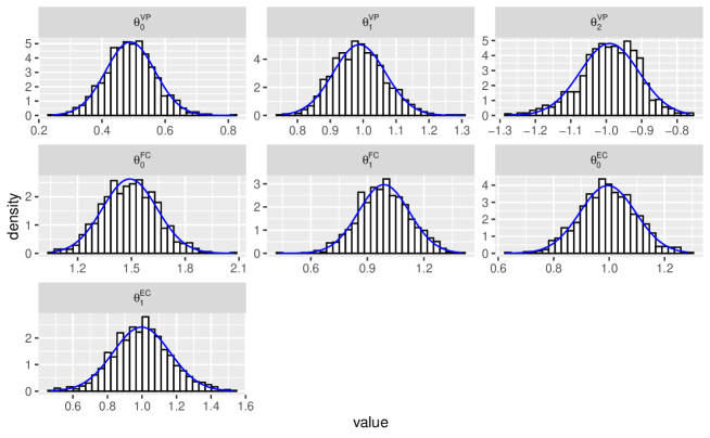
Note: Histograms denote the finite sample distribution, and blue line is normal density

Figure B.1. Finite sample distributions under linear semi-gradients without locally robust corrections.

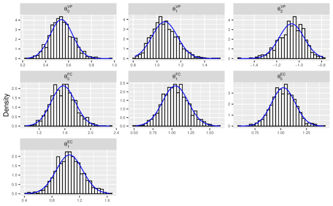
Note: Histograms denote the finite sample distribution, and blue line is normal density

Figure B.2. Finite sample distributions under linear semi-gradients with locally robust corrections.

Figures B.3 and B.4 present similar results for AVI.

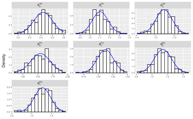
Note: Histograms denote the finite sample distribution, and blue line is normal density

Figure B.3. Finite sample distributions under AVI without locally robust corrections.

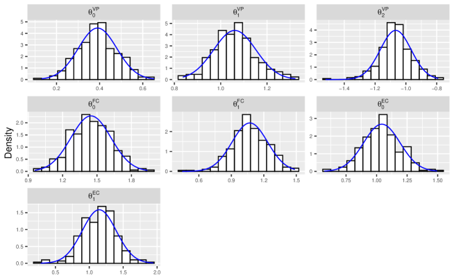
Note: Histograms denote the finite sample distribution, and blue line is normal density

Figure B.4. Finite sample distributions under AVI with locally robust corrections.

B.7.2. Bus engine replacement problem

Consider the following version of the Rust (1987) bus engine replacement problem which is adapted from Arcidiacono and Miller (2011). Each period $t=1,...,T;T<\infty$, Harold Zurcher decides whether to replace the engine of a bus ($a_{t}=0$), or keep it ($a_{t}=1$). Denote his action by $j\in\{0,1\}$. Each bus is characterized by a permanent type $s\in\{1,2\}$, and the mileage accumulated since the last engine replacement $x_{t}\in\{1,2,...\}$. Harold Zurcher observes both $s$ and $x_{t}$. The econometrician observes mileage $x_{t}$, and we make different assumptions on the observability of bus type $s$.

Mileage increases by one unit if the engine is kept in period $t$ and is set to zero if the engine is replaced. The current-period payoff for keeping the engine is given by $\theta_{0}+\theta_{1}x_{t}+\theta_{2}s+e_{1t}$, where $\theta^{*}\equiv\{\theta_{0},\theta_{1},\theta_{2}\}$ are the structural parameters of interest, and $e_{jt}$ is a choice-specific transitory shock that follows a Type 1 Extreme Value distribution. The current-period payoff of replacing the engine is normalized to $e_{0t}$, and the discount factor is set to 0.9 in this application.

To carry out the simulations, we choose values for the structural parameters ($\theta_{0}=2,\theta_{1}=-0.15,\theta_{2}=1$), and recursively derive the value functions for each possible combination of $x$, $s$ and $t$. We then use these to compute the conditional replacement probabilities for the same set of combinations of variables.

We provide results using the linear semi-gradient method to approximate $h(a,x)$ and $g(a,x)$. Our first set of results treats the bus type $s$ as known to the econometrician. We then provide findings for a setting with permanent unobserved heterogeneity. All results are based on $1000$ simulations with $1000$ buses and $T=30$ time periods each. Each round of the simulations begins by generating data for $1000$ buses and $2000$ time periods. The mileage of each bus is set to zero in $t=0$. We then simulate the choices $a_{t}$ using the conditional replacement probabilities. Finally, we restrict the generated data to $30$ time periods between $t=1000$ and $t=1030$. This is to ensure that our data is close to being drawn from a stationary model. In all simulations, we parameterize $h(a,x)$ and $g(a,x)$ using a third order polynomial in $s$, $x_{t}$ and $a_{t}$. The choice probabilities $\eta$ are estimated using a logit model that is a function of the state variables $s$ and $x_{t}$, where the same polynomial is used as before.

Table B.1 shows the results treating bus type $s$ as known, with and without locally robust correction. It can be seen that our estimator produces parameter estimates that are closely centered around the true values. These results are comparable to those found by Arcidiacono and Miller (2011) in a similar version of the bus engine replacement problem. However, in contrast to their CCP method, our estimator does not exploit a finite dependence property. When comparing the results from our locally robust estimator in column (4) to the results from the suboptimal estimator in column $(2)$, it can be seen that the absolute bias is smaller for all three parameter estimates. However the variance of the locally robust estimator is higher due to the sample splitting employed in the locally robust procedure (we used two-fold cross-fitting). Overall, while in theory the locally robust estimator is preferable to the non-robust version, we find that in practice there is very little difference between the two versions of the algorithm.

Table B.1. Simulations: Bus engine replacement problem

			not locally robust			locally robust
	DGP		TDL	MSE		TDL	MSE
	(1)		(2)	(3)		(4)	(5)
Linear semi-gradient
$\theta_{0}$ (intercept)	2.0		1.9788	0.0080		1.9778	0.0081
			(0.0868)			(0.0870)
$\theta_{1}$ (mileage)	-0.15		-0.1492	1.2e-05		-0.1489	1.3e-05
			(0.0033)			(0.0034)
$\theta_{2}$ (bus type)	1.0		1.0044	0.0034		1.0032	0.0034
			(0.0583)			(0.0584)

Notes: The table reports results for 1000 simulations. Column (1) shows the true parameter values in the model. Columns (2) and (4) report the empirical mean and standard deviations for the estimated parameters. Columns (2)-(3) are based on the estimation method without correction function, columns (4)-(5) report results for the locally robust estimator. The mean squared error are reported in columns (3) and (5), respectively.

In a final set of simulations, we introduce permanent unobserved heterogeneity into our setting by assuming that the permanent bus type $s\in\{1,2\}$ is unknown to the researcher. To generate results for these simulations, we follow the steps outlined in Section B.6 where we pair our techniques with a sequential EM algorithm (Arcidiacono and Jones, 2003), without using a locally robust correction. The results are shown in Table B.2. Once again, our algorithm produces parameter estimates that are closely centered around the true values. Compared to the results without permanent unobserved heterogeneity, the standard deviation of our estimates is slightly higher due to the uncertainty around the bus type $s$.

Table B.2. Simulations: Bus engine replacement problem with unobserved heterogeneity

	DGP		TDL	MSE
	(1)		(2)	(3)
Linear semi-gradient
$\theta_{0}$ (intercept)	2.0		1.9750	0.0164
			(0.1255)
$\theta_{1}$ (mileage)	-0.15		-0.1492	1.5e-05
			(0.0039)
$\theta_{2}$ (bus type)	1.0		1.0035	0.0104
			(0.1018)

Notes: The table reports results for 1000 simulations. Column (1) shows the true parameter values in the model. Column (2) reports the empirical mean and standard deviations for the estimated parameters. The mean squared errors are reported in column (3). The results are based on the estimation method without correction function.

References

- Ackerberg et al. (2014) D. Ackerberg, X. Chen, J. Hahn, and Z. Liao, “Asymptotic efficiency of semiparametric two-step gmm,” Review of Economic Studies, vol. 81, no. 3, pp. 919–943, 2014.
- Aguirregabiria and Magesan (2018) V. Aguirregabiria and A. Magesan, “Solution and estimation of dynamic discrete choice structural models using euler equations,” Working paper, 2018.
- Aguirregabiria and Mira (2002) V. Aguirregabiria and P. Mira, “Swapping the nested fixed point algorithm: A class of estimators for discrete markov decision models,” Econometrica, vol. 70, no. 4, pp. 1519–1543, 2002.
- Aguirregabiria and Mira (2007) ——, “Sequential estimation of dynamic discrete games,” Econometrica, vol. 75, no. 1, pp. 1–53, 2007.
- Aguirregabiria and Mira (2010) ——, “Dynamic discrete choice structural models: A survey,” Journal of Econometrics, vol. 156, no. 1, pp. 38–67, 2010.
- Almagro and Domınguez-Iino (2019) M. Almagro and T. Domınguez-Iino, “Location sorting and endogenous amenities: Evidence from amsterdam,” NYU, mimeograph, 2019.
- Arcidiacono and Jones (2003) P. Arcidiacono and J. B. Jones, “Finite mixture distributions, sequential likelihood and the em algorithm,” Econometrica, vol. 71, no. 3, pp. 933–946, 2003.
- Arcidiacono and Miller (2011) P. Arcidiacono and R. A. Miller, “Conditional choice probability estimation of dynamic discrete choice models with unobserved heterogeneity,” Econometrica, vol. 79, no. 6, pp. 1823–1867, 2011.
- Arcidiacono et al. (2013) P. Arcidiacono, P. Bayer, F. A. Bugni, and J. James, “Approximating high-dimensional dynamic models: Sieve value function iteration,” in Structural Econometric Models. Emerald Group Publishing Limited, 2013, pp. 45–95.
- Bajari et al. (2007) P. Bajari, C. L. Bankard, and J. Levin, “Estimating dynamic models of imperfect competition,” Econometrica, vol. 75, no. 5, pp. 1331–1370, 2007.
- Barwick and Pathak (2015) P. J. Barwick and P. A. Pathak, “The costs of free entry: an empirical study of real estate agents in greater boston,” The RAND Journal of Economics, vol. 46, no. 1, pp. 103–145, 2015.
- Biau (2012) G. Biau, “Analysis of a random forests model,” The Journal of Machine Learning Research, vol. 13, pp. 1063–1095, 2012.
- Chernozhukov et al. (2018) V. Chernozhukov, W. K. Newey, and R. Singh, “Learning l2 continuous regression functionals via regularized riesz representers,” arXiv preprint arXiv:1809.05224, vol. 8, 2018.