Hamiltonian Tomography via Quantum Quench

Abstract

We show that it is possible to uniquely reconstruct a generic many-body local Hamiltonian from a single pair of generic initial and final states related by evolving with the Hamiltonian for any time interval. We then propose a practical version of the protocol involving multiple pairs of such initial and final states. Using the eigenstate thermalization hypothesis, we provide bounds on the protocol’s performance and stability against errors from measurements and in the ansatz of the Hamiltonian. The protocol is efficient (requiring experimental resources scaling polynomially with system size in general and constant with system size given translation symmetry) and thus enables analog and digital quantum simulators to verify implementation of a putative Hamiltonian.

The advent of quantum many-body simulators Blatt and Roos (2012); Zhang et al. (2017); Islam et al. (2013); Devoret and Schoelkopf (2013); Gambetta et al. (2017); Greiner et al. (2002); Bloch et al. (2008); Bernien et al. (2017); Jördens et al. (2008); Gross and Bloch (2017); Mazurenko et al. (2017); Chiaro et al. (2019) has enabled the exploration of complex quantum dynamics beyond the capabilities of classical computers. Given this significant potential, it is vital to determine accurately the Hamiltonian actually being realized by a simulator. However, Hamiltonian tomography for a generic many-body system is challenging, precisely due to the fact that the complexity of many-body dynamics makes benchmarking with a classical computer difficult. Thus far, most progress has been made in systems with either a special Hamiltonian or a small size Schirmer et al. (2004); Devitt et al. (2006); Cole et al. (2005, 2006); Di Franco et al. (2009); Burgarth and Maruyama (2009); Burgarth et al. (2009, 2011); da Silva et al. (2011); Senko et al. (2014); Zhang and Sarovar (2014); Wiebe et al. (2014); Wang et al. (2015); Ma et al. (2017); Hauke et al. (2014); Jurcevic et al. (2015).

In this Letter, we introduce two protocols for Hamiltonian tomography (Fig. 1). The first is more of conceptual interest: we show that it is possible to uniquely reconstruct a generic many-body Hamiltonian with local interactions given only a single pair of generic initial and final states connected by time evolving with the Hamiltonian. Our approach is partly motivated by the recent proposals of reconstructing a many-body Hamiltonian from a single eigenstate or steady state Garrison and Grover (2018); Qi and Ranard (2019); Chertkov and Clark (2018); Bairey et al. (2019); Evans et al. (2019). As in these studies, our protocol relies on the physical assumption that the Hamiltonian is local, which implies that the number of its parameters scales polynomially with system size. However, in contrast to these works, our approach does not require a steady state and instead relies precisely on how a generic state changes in time.

Despite being conceptually interesting, this first protocol is impractical and we thus propose a second, practical version that uses multiple pairs of initial and final states connected by time evolving with the Hamiltonian. This protocol only requires measuring a set of local observables in each pair of initial and final states. We bound the errors in the reconstructed Hamiltonian due to errors in both the measurements and the ansatz of the Hamiltonian, and the fidelity of the reconstruction can be increased to unity by using more pairs of initial-final states.

We emphasize that our locality assumption does not necessarily have to be spatial locality; we only require that all interactions in the Hamiltonian involve a fixed number of degrees of freedom that is independent of system size. Hence, our protocol applies to all analog and digital quantum simulators, from superconducting circuits to trapped ion platforms. We only require measurement of local observables, which can be done with high precision thanks to recent advances in single-site resolution.

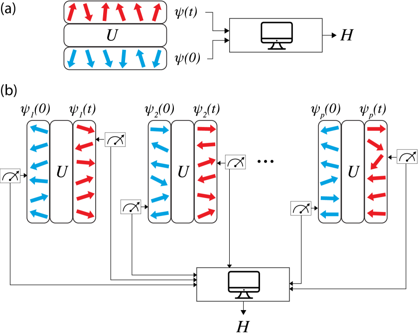
Figure 1: Two protocols for Hamiltonian tomography. (a) From a single pair of initial and final states related by time evolving with the Hamiltonian, $|\psi(t)\rangle=U|\psi(0)\rangle$ with $U=\exp\left(-iHt\right)$, a generic Hamiltonian can be uniquely reconstructed. (b) A practical version using $p$ pairs of initial and final states related by time evolving with the Hamiltonian and requiring only local measurements on the initial and final states.

Tomography from a single quench.—Given a Hamiltonian $H$ and an initial state $\ket{\psi(0)}$ of a $D$-dimensional Hilbert space, we ask whether one can determine $H$ from only $\ket{\psi(0)}$ and $\ket{\psi(t)}=e^{-iHt}\ket{\psi(0)}$. Without any restrictions, it is impossible to determine $H$ uniquely, since $H$ has $O(D^{2})$ parameters while the given wave functions contain $O(D)$ parameters. However, a many-body Hamiltonian with local interactions has number of parameters scaling polynomially with system size, $L$, whereas $D$ is exponential in $L$, and thus reconstructing a local $H$ is possible in principle.

Without loss of generality, we consider a traceless many-body Hamiltonian and decompose it into $n$ local interaction terms:

$$H=\sum_{\alpha=1}^{n}c_{\alpha}\mathcal{O}_{\alpha},$$ (1)

where $\{\mathcal{O}_{\alpha}\}$ are traceless local Hermitian operators, $\{c_{\alpha}\}$ are coupling constants, and $n$ is a polynomial of $L$ due to locality. Our goal is to determine $\{c_{\alpha}\}$ from $\ket{\psi(0)}$ and $\ket{\psi(t)}=e^{-iHt}\ket{\psi(0)}$.

Our approach is based on the simple observation of generalized energy conservation:

$$\bra{\psi(t)}H^{m}\ket{\psi(t)}=\bra{\psi(0)}H^{m}\ket{\psi(0)}$$ (2)

for any positive integer $m$. These equations place many constraints on the variables $\{c_{\alpha}\}$. Indeed, substituting Eq. (1) (with $c$ replaced by $x$, a symbol for unknowns) into Eq. (2) yields (repeated indices summed over):

$$M^{(m)}_{\alpha_{1}\alpha_{2}\cdots\alpha_{m}}x_{\alpha_{1}}x_{\alpha_{2}}...x_{\alpha_{m}}=0,$$ (3)

where

$$M^{(m)}_{\alpha_{1}\alpha_{2}\cdots\alpha_{m}}= \bra{\psi(0)}\mathcal{O}_{\alpha_{1}}\mathcal{O}_{\alpha_{2}}\cdots\mathcal{O}_{\alpha_{m}}\ket{\psi(0)}$$ (4)

$$-\bra{\psi(t)}\mathcal{O}_{\alpha_{1}}\mathcal{O}_{\alpha_{2}}\cdots\mathcal{O}_{\alpha_{m}}\ket{\psi(t)}.$$

More explicitly, we have $M^{(1)}_{\alpha_{1}}x_{\alpha_{1}}=0,M^{(2)}_{\alpha_{1}\alpha_{2}}x_{\alpha_{1}}x_{\alpha_{2}}=0$, etc., which we refer to as first order, second order, etc. This constitutes a system of polynomial equations for $\{x_{\alpha}\}$ which can be used to determine $\{c_{\alpha}\}$ (and thus $H$). Note that without knowledge of $t$, one can always rescale $H$ and $t$ to leave $Ht$ invariant, so $\{c_{\alpha}\}$ will be determined up to an overall multiplicative factor. Hereafter we omit the “up to a factor” caveat.

Although Eq. (2) is valid for any positive integer $m$, it can be shown sup that at most $(D-1)$ of these equations are independent. As long as $D-1\geqslant n$, our procedure uses the first $n$ equations ($m=1,2\cdots n$) to determine $\{c_{\alpha}\}$. We find that if there exists one example of a Hamiltonian, $H_{0}$, that can be uniquely reconstructed from this procedure, then a generic Hamiltonian can be uniquely reconstructed from this procedure. The proof of our claim is based on the analytic properties of resultants of polynomial equations, and we leave the technical details to the Supplementary Material sup . There we also show that given the time $t$ as an additional input, a generic $H$ can be determined completely (including the overall scale).

Our procedure applies to generic Hamiltonians and initial states, and it can be immediately generalized for mixed initial states. However, there will be fine-tuned cases for which it fails. For example, if $|\psi(0)\rangle$ is an eigenstate of $H$, Eq. (2) is trivially satisfied and we cannot obtain $H$ from it. Nevertheless, in this special case one can in principle employ the methods in Refs. Garrison and Grover (2018); Qi and Ranard (2019); Chertkov and Clark (2018); Bairey et al. (2019); Evans et al. (2019) to determine the Hamiltonian. Furthermore, if $H$ admits a conserved quantity $Q$ that can be decomposed into the same set of local operators, $\{\mathcal{O}_{\alpha}\}$, then Eq. (2) yields any linear combination of $H$ and $Q$.

Proof of concept.—In order to demonstrate uniqueness for generic cases, one needs to show the existence of $H_{0}$ for arbitrary system size, which is a difficult problem. In this Letter, we present three physically relevant checks.

The first is an analytical check on a spin-$1/2$ chain. We consider a translationally invariant transverse-field Ising model with three random couplings:

$$H=c_{1}\sum_{i}Z_{i}Z_{i+1}+c_{2}\sum_{i}X_{i}+c_{3}\sum_{i}Y_{i}Y_{i+2},$$ (5)

in which $X,Y,Z$ are Pauli operators. We have added a next-nearest-neighbor interaction; otherwise, the problem is trivial and the first order (linear) equation in Eq. (3) is enough to determine $c_{1}/c_{2}$. Using a small $t$ approximation, it can be analytically shown sup that the first and second order equations have two solutions, only one of which satisfies the third order equation, and this unique reconstruction for small $t$ is sufficient to establish unique reconstruction for finite $t$. We emphasize that the small $t$ approximation is not a requirement of our protocol; it is an intermediate step in establishing the uniqueness of reconstruction.

We also numerically check reconstruction using finite time evolution for similar models. For example, we check the Ising model with transverse and longitudinal fields and the Heisenberg model for chains up to length $L=10$:

$$H =c_{1}\sum_{i=1}^{L-1}Z_{i}Z_{i+1}+c_{2}\sum_{i=1}^{L}X_{i}+c_{3}\sum_{i=1}^{L}Z_{i},$$ (6)

$$H =c_{1}\sum_{i=1}^{L-1}X_{i}X_{i+1}+c_{2}\sum_{i=1}^{L-1}Y_{i}Y_{i+1}+c_{3}\sum_{i=1}^{L-1}Z_{i}Z_{i+1}.$$

We find similar uniqueness results as above.

The third check is closer to a generic Hamiltonian. We consider a transverse field Ising model with random spatially varying couplings $c_{1,i}$ and $c_{2,i}$:

$$H=\sum_{i=1}^{L}c_{1,i}X_{i}+\sum_{i=1}^{L-1}c_{2,i}Z_{i}Z_{i+1}$$ (7)

Due to the high computational complexity [the number of coefficients in Eq. (3) is exponential in $n$], we only check the case of $L=4$ (7 local operators in total) for illustration. Using the Gröbner basis Cox et al. (2015) technique, we find that $n=7$ polynomial equations indeed determine $\{c\}$ uniquely.

The above checks provide evidence for the existence of $H_{0}$ for various classes of Hamiltonians, which strongly suggests that a generic local many-body Hamiltonian can be uniquely reconstructed from a single pair of initial-final states related via time evolving with the Hamiltonian.

Reconstruction from multiple quenches.—Though the above protocol is conceptually interesting, it is impractical because the experimental and computational complexity are both exponential in $n$. Hence, below we present a more practical method for Hamiltonian tomography, whose experimental and computational complexity is only a polynomial of $n$ and whose sensitivity to errors can be controlled.

Since the high complexity of the first approach arises from the higher order equations [$m\geqslant 2$ in Eq. (3)], we will only keep the linear equation $(m=1)$. In order to uniquely determine $\{c_{\alpha}\}$, we need at least $(n-1)$ linear equations. Hence we use $p\geqslant(n-1)$ pairs of initial and final states related by time evolving with $H$:

$$\{\ket{\psi_{i}(0)}\to\ket{\psi_{i}(t)}=e^{-iHt}\ket{\psi_{i}(0)},~{}i=1,2\cdots p\},$$ (8)

As a result, we have a linear system of equations $Mx=0$, where $M$ is a $p\times n$ matrix with entries

$$M_{i\alpha}=\bra{\psi_{i}(0)}\mathcal{O}_{\alpha}\ket{\psi_{i}(0)}-\bra{\psi_{i}(t)}\mathcal{O}_{\alpha}\ket{\psi_{i}(t)}.$$ (9)

In principle it is sufficient to use $p=n-1$, and the kernel of $M$ will generically be one dimensional and equal to $\{c_{\alpha}\}$. (The uniqueness can be addressed by the same technique as for the single quench protocol.) In contrast to the first approach, the number of measurements required is proportional to the number of coefficients in $M$, which is $O(n^{2})$.

Inevitably there will be experimental errors in state preparation, time evolution, and measurements, and these will lead to errors in the reconstructed Hamiltonian. We can mitigate these errors by utilizing more than $(n-1)$ pairs of initial-final states. Using $p>n-1$, we want to find the best fit of $\{x\}$ for $Mx=0$ when $M_{i\alpha}$ has random error. We use the standard least squares method for a homogeneous system of equations: the best estimate of $\{x\}$ is given by the right singular vector of $M$ with the smallest singular value (or equivalently, the eigenvector of $M^{T}M$ with the smallest eigenvalue). A similar approach was used in Ref. Bentsen et al. (2019) to find local integrals of motion; however, while that approach used different time slices from evolving a fixed initial state, our approach fixes one time and uses different pairs of initial and final states, which leads to more efficient use of experimental resources, as we will discuss below.

Stability against measurement errors.—To quantify the error in the reconstructed Hamiltonian $H=\sum_{\alpha}x_{\alpha}\mathcal{O}_{\alpha}$, we define $\theta$ to be the angle between the vector of reconstructed coupling constants $x$ and the vector of actual coupling constants $c$, and correspondingly the fidelity $F=|\cos\theta|$ and reconstruction error $E=|\sin\theta|$.

Consider an error model in which each matrix element $M_{i\alpha}$ has an additive error uniformly distributed between $\pm\epsilon$. Using both standard perturbation theory and nonperturbative results in statistical theory Cai and Zhang (2018), we find that the average reconstruction error is bounded:

$$E\leqslant C\sqrt{\frac{n}{p}}\frac{\epsilon}{\lambda}$$ (10)

for $\epsilon<\lambda$, where $C$ is a constant and $\lambda$ is the gap between the two lowest singular values of $\frac{1}{\sqrt{p}}M$ ($\lambda$ becomes independent of $p$ as $p\rightarrow\infty$) sup .

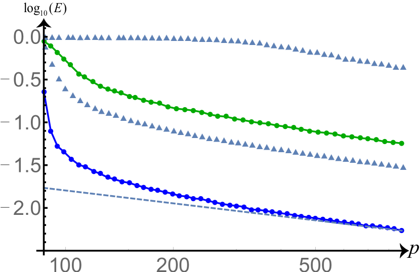
Figure 2: Reconstruction error vs number of initial and final pairs on log-log plot for $L=8,~{}t=1$ and error $\epsilon=0.1$ (green) and $\epsilon=0.01$ (blue). The gray triangles denote reconstruction error from the procedure in Ref. Bentsen et al. (2019), using $p$ different time slices separated by $dt=1$ and one fixed initial state, for $\epsilon=0.1$ (top) and $\epsilon=0.01$ (middle). Each point here is averaged over 200 realizations of error and random Hamiltonian Eq. (13) with couplings chosen from $(-1,1)$. The reference dashed line (bottom) corresponds to $E\propto\frac{1}{\sqrt{p}}$ predicted by Eq. (10). Note that the initial decrease in error is steeper than the final rate.

Therefore, by increasing the number of pairs of initial-final states, $p$, one can decrease the reconstruction error . As Eq. (10) implies, we would like $\lambda$ to be as large as possible. The gap is determined by $M$, which in turn depends on the important choices of time $t$ and the ensemble of initial states. Intuitively, larger $t$ is preferable so that the initial and final states are more distinguishable in terms of local observables. In the same vein, the initial states should not be too random; otherwise, the time evolution has little effect on changing local observables (for example, we find that Haar random initial states perform poorly). At the same time, states in the initial ensemble should be distinct enough to provide independent information about $H$.

We now discuss the dependence of $\lambda$ on these factors in more details. To understand the singular values of $\frac{1}{\sqrt{p}}M$, we note that

$$\left(\frac{1}{p}M^{T}M\right)_{\alpha\beta}\!\!=\overline{\bra{\psi}\mathcal{O}_{\alpha}-\mathcal{O}_{\alpha}(t)\ket{\psi}\bra{\psi}\mathcal{O}_{\beta}-\mathcal{O}_{\beta}(t)\ket{\psi}},$$ (11)

where the overline denotes an average over the initial state ensemble. We find that choosing the initial states from an ensemble of random product states provides a robust (and experimentally practical) scheme. Specifically, for a system of qubits we consider initial states given by

$$\ket{\psi(0)}=\prod_{i}\ket{\phi_{i}},$$ (12)

with $\ket{\phi_{i}}$ a random state on the Bloch sphere at site $i$. (Alternatively, for each site one can choose $\ket{\phi_{i}}=|\pm 1\rangle$ in either the $X$,$Y$, or $Z$ basis.) Our results hereafter will assume the random Bloch sphere states as the initial states.

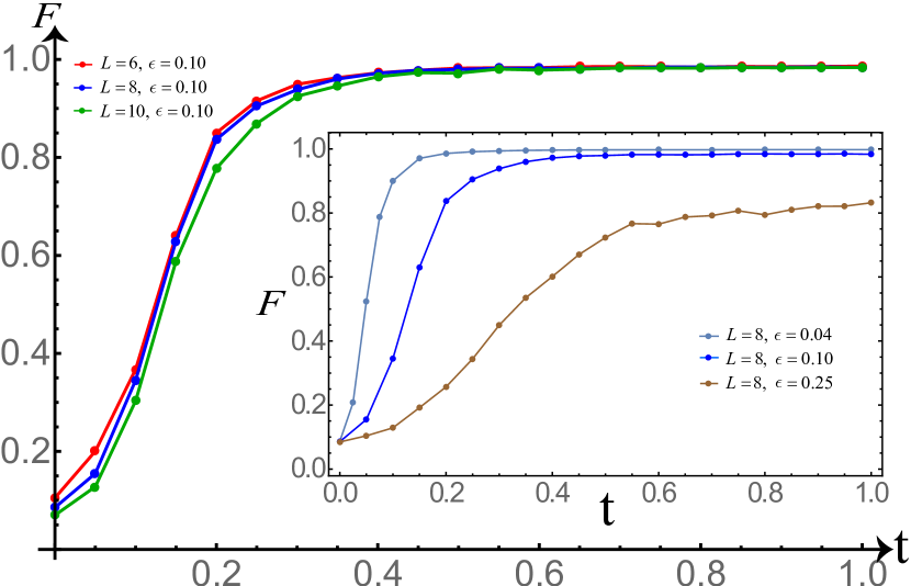
Figure 3: Reconstruction fidelity as a function of time interval $t$. We fix $p=2n$. Each point here is averaged over 200 realizations of error and random Hamiltonian Eq. (13) with couplings chosen from $(-1,1)$. In the main figure, three curves correspond to $L=6,8,10$ with errors in $(-0.1,0.1)$. In the subfigure, three curves correspond to errors in $(-0.04,0.04)$, $(-0.1,0.1)$, and $(-0.25,0.25)$, with $L=8$.

We analyze a generic class of Hamiltonians with random onsite and nearest-neighbor interactions in a spin$-1/2$ chain:

$$H=\sum_{i=1}^{L}\sum_{a=1}^{3}c_{ia}\sigma_{i}^{a}+\sum_{i=1}^{L-1}\sum_{a,b=1}^{3}c_{iab}\sigma_{i}^{a}\sigma_{i+1}^{b}.$$ (13)

Here $c_{ia}$ and $c_{iab}$ are random variables and $\sigma^{1,2,3}=\{X,Y,Z\}$ are Pauli operators. We will average over random Hamiltonian realizations $c_{ia},c_{iab}\in(-1,1)$ and error realizations in $(-\epsilon,\epsilon)$. In Fig. 2, we plot the reconstruction error vs. $p$ and confirm the $1/{\sqrt{p}}$ dependence in Eq. (10). We use the experimentally reasonable timescale $t=1$ for $L=8$ and observe that $p=2n$ number of pairs is sufficient to achieve a high fidelity of 0.98 when $\epsilon=0.1$.

Figure 2 also shows that our approach performs substantially better than evolving a fixed initial state with different times. This is because in the latter approach, if the times are too large, the final states will be locally thermal and hardly distinguishable. On the other hand, states separated by small time are also hard to distinguish. Using these states in Eq. (9) would result in $M$ and its gap $\lambda$ being smaller. This is also evident when we use our method and choose a small $t$ (see reconstruction fidelity versus $t$ in Fig. 3; the fidelity at $t\approx 0$ is nonzero because the overlap between two random vectors in $\mathbb{R}^{n}$ is roughly $\frac{1}{\sqrt{n}}$). It is only at later times that $M$ and $\lambda$ become sufficiently nonzero, and the fidelity approaches unity.

To understand the behavior of the fidelity curve in Fig. 3 and in particular its late time value, we have the following result. Consider the correlation function $C_{\alpha\beta}(t)=\frac{1}{D}{\rm Tr}[\mathcal{O}_{\alpha}(0)\mathcal{O}_{\beta}(t)]$ (an $n\times n$ matrix) and let $l_{\max}$ be the maximum size of an operator in $\{\mathcal{O}_{\alpha}\}$. For example, the operator $Z_{i}Z_{j}$ has size $2$ regardless of the distance $|i-j|$; a local Hamiltonian has $l_{\max}$ of $O(1)$. Using Eq. (11) and analyzing operator growth sup , we find

$$\lambda(t)\geqslant\left(\frac{1}{3}\right)^{l_{\max}/2}s_{2}\left(I-C(t)\right),$$ (14)

where $s_{2}(I-C(t))$ denotes the 2nd smallest singular value of $I-C(t)$. Due to operator scrambling, we expect $C(t)$ to decay in time; assuming the eigenstate thermalization hypothesis (ETH), matrix elements of $C(\infty)$ are $O(\frac{1}{L})$ Huang et al. (2019) with fluctuations exponentially small in system size Alhambra et al. (2020). We use similar techniques to find that $s_{2}(I-C(\infty))\geqslant 1-O(1/L)$. Eq. (14) thus provides an $O(1)$ lower bound for the gap.

We emphasize that the above lower bound is independent of system size. Indeed, we find in Fig. 3 that the late time reconstruction fidelity is insensitive to system size. However, the time scale at which the maximal fidelity is reached depends on the time scale at which $C(t)$ asymptotes, which is expected to increase at most polynomially with system size. Note that the fidelity timescale also depends on the error magnitude: in the limit of zero error, the timescale for saturation approaches zero. We observe in the numerics that for experimentally reasonable $L=10$, error $\epsilon=0.1$, and pairs of states $p=2n$, an $O(1)$ time is more than sufficient to reach maximal fidelity.

Stability against errors in the ansatz of the Hamiltonian.—In reality, interactions are not strictly compactly supported; there are small nonlocal interactions. This motivates consideration of an enlarged Hamiltonian

$$H=\sum_{\alpha}c_{\alpha}\mathcal{O}_{\alpha}+\sum_{\beta}c^{\prime}_{\beta}\mathcal{O}^{\prime}_{\beta}$$ (15)

in which the support of $\mathcal{O}^{\prime}_{\beta}$ is not necessarily bounded, but we assume $\left\lVert c^{\prime}\right\rVert\ll\left\lVert c\right\rVert$.

Restricted by experimental and computational resources, it is desirable to model only the dominant interactions. Assuming the real Hamiltonian is described by Eq. (15) and we use our method to reconstruct an “effective” Hamiltonian $H=\sum_{\alpha}x_{\alpha}\mathcal{O}_{\alpha}$, how different will $x$ be from $c$?

The matrix in Eq. (9) now consists of two pieces $(M;M^{\prime})$ from $\{\mathcal{O}_{\alpha}\},\{\mathcal{O}^{\prime}_{\beta}\}$ respectively. The actual coefficient vector $\begin{pmatrix}c\\ c^{\prime}\end{pmatrix}$ is the singular vector of $(M;M^{\prime})$ with singular value 0. By restricting the operator set to $\{\mathcal{O}_{\alpha}\}$, one only measures $M$ and calculates its minimal singular vector $x$.

We find sup that the reconstruction error between $x,c$ is controlled by

$$E\leqslant\frac{\left\lVert\frac{1}{\sqrt{p}}M^{\prime}\right\rVert}{s_{2}\left(\sqrt{\frac{1}{p}}M\right)}\frac{\left\lVert c^{\prime}\right\rVert}{\left\lVert c\right\rVert}.$$ (16)

Recall that $s_{2}(\sqrt{\frac{1}{p}}M)$ denotes the second smallest singular value of $\frac{1}{\sqrt{p}}M$. Using ETH, we show that $s_{2}(\sqrt{\frac{1}{p}}M)\geqslant(\frac{1}{3})^{l_{\max}/2}-O(\frac{1}{L})$, where $l_{\max}$ is the size of the largest operator in $\{\mathcal{O}_{\alpha}\}$ (not $\{\mathcal{O}^{\prime}_{\beta}\}$). Therefore $(\frac{1}{3})^{l_{\max}/2}$ is $O(1)$ and does not vanish even though the full Hamiltonian may contain arbitrarily nonlocal operators. We also show that $\left\lVert\frac{1}{\sqrt{p}}M^{\prime}\right\rVert$ has an $O(1)$ bound. Thus, as long as $\left\lVert c^{\prime}\right\rVert\ll\left\lVert c\right\rVert$, our reconstruction will succeed.

Summary.—We have shown that a single quantum quench is sufficient in principle to reconstruct a generic many-body Hamiltonian with local interactions. We also propose a practical version involving multiple quantum quenches from random initial product states and requiring only measurement of local observables. Using ETH, we analytically bound the reconstruction error arising from measurement errors and ignorance of nonlocal interactions. The efficiency and robustness of our protocol enable quantum simulators to determine precisely the Hamiltonian being implemented.

Acknowledgements.—We thank Álvaro Alhambra, Ehud Altman, Xiaoliang Qi, and Beni Yoshida for helpful discussions, and Gabriela Secara for help with figure design. Z.L. is grateful for the hospitality of the Visiting Graduate Fellowship program at Perimeter Institute where this work was carried out. Z.L. is also supported by the PQI fellowship from Pittsburgh Quantum Institution. L.Z. is supported by the John Bardeen Postdoctoral Fellowship. Research at Perimeter Institute is supported in part by the Government of Canada through the Department of Innovation, Science and Economic Development Canada and by the Province of Ontario through the Ministry of Colleges and Universities.

References

- Blatt and Roos (2012) R. Blatt and C. F. Roos, “Quantum simulations with trapped ions,” Nature Physics 8, 277–284 (2012).
- Zhang et al. (2017) J. Zhang, G. Pagano, P. W. Hess, A. Kyprianidis, P. Becker, H. Kaplan, A. V. Gorshkov, Z.-X. Gong, and C. Monroe, “Observation of a many-body dynamical phase transition with a 53-qubit quantum simulator,” Nature 551, 601–604 (2017).
- Islam et al. (2013) R. Islam, C. Senko, W. C. Campbell, S. Korenblit, J. Smith, A. Lee, E. E. Edwards, C.-C. J. Wang, J. K. Freericks, and C. Monroe, “Emergence and frustration of magnetism with variable-range interactions in a quantum simulator,” Science 340, 583–587 (2013).
- Devoret and Schoelkopf (2013) M. H. Devoret and R. J. Schoelkopf, “Superconducting circuits for quantum information: an outlook,” Science 339, 1169 (2013).
- Gambetta et al. (2017) Jay M. Gambetta, Jerry M. Chow, and Matthias Steffen, “Building logical qubits in a superconducting quantum computing system,” npj Quantum Information 3, 2 (2017).
- Greiner et al. (2002) Markus Greiner, Olaf Mandel, Tilman Esslinger, Theodor W. Hänsch, and Immanuel Bloch, “Quantum phase transition from a superfluid to a mott insulator in a gas of ultracold atoms,” Nature 415, 39–44 (2002).
- Bloch et al. (2008) Immanuel Bloch, Jean Dalibard, and Wilhelm Zwerger, “Many-body physics with ultracold gases,” Rev. Mod. Phys. 80, 885–964 (2008).
- Bernien et al. (2017) Hannes Bernien, Sylvain Schwartz, Alexander Keesling, Harry Levine, Ahmed Omran, Hannes Pichler, Soonwon Choi, Alexander S. Zibrov, Manuel Endres, Markus Greiner, Vladan Vuletić, and Mikhail D. Lukin, “Probing many-body dynamics on a 51-atom quantum simulator,” Nature 551, 579–584 (2017).
- Jördens et al. (2008) Robert Jördens, Niels Strohmaier, Kenneth Günter, Henning Moritz, and Tilman Esslinger, “A mott insulator of fermionic atoms in an optical lattice,” Nature 455, 204 EP – (2008).
- Gross and Bloch (2017) Christian Gross and Immanuel Bloch, “Quantum simulations with ultracold atoms in optical lattices,” Science 357, 995–1001 (2017).
- Mazurenko et al. (2017) Anton Mazurenko, Christie S. Chiu, Geoffrey Ji, Maxwell F. Parsons, Márton Kanász-Nagy, Richard Schmidt, Fabian Grusdt, Eugene Demler, Daniel Greif, and Markus Greiner, “A cold-atom fermi–hubbard antiferromagnet,” Nature 545, 462–466 (2017).
- Chiaro et al. (2019) B. Chiaro et al., “Growth and preservation of entanglement in a many-body localized system,” (2019), arXiv:1910.06024 [cond-mat.dis-nn] .
- Schirmer et al. (2004) S. G. Schirmer, A. Kolli, and D. K. L. Oi, “Experimental hamiltonian identification for controlled two-level systems,” Phys. Rev. A 69, 050306 (2004).
- Devitt et al. (2006) Simon J. Devitt, Jared H. Cole, and Lloyd C. L. Hollenberg, “Scheme for direct measurement of a general two-qubit hamiltonian,” Phys. Rev. A 73, 052317 (2006).
- Cole et al. (2005) Jared H. Cole, Sonia G. Schirmer, Andrew D. Greentree, Cameron J. Wellard, Daniel K. L. Oi, and Lloyd C. L. Hollenberg, “Identifying an experimental two-state hamiltonian to arbitrary accuracy,” Phys. Rev. A 71, 062312 (2005).
- Cole et al. (2006) Jared H Cole, Simon J Devitt, and Lloyd C L Hollenberg, “Precision characterization of two-qubit hamiltonians via entanglement mapping,” Journal of Physics A: Mathematical and General 39, 14649–14658 (2006).
- Di Franco et al. (2009) C. Di Franco, M. Paternostro, and M. S. Kim, “Hamiltonian tomography in an access-limited setting without state initialization,” Phys. Rev. Lett. 102, 187203 (2009).
- Burgarth and Maruyama (2009) Daniel Burgarth and Koji Maruyama, “Indirect hamiltonian identification through a small gateway,” New Journal of Physics 11, 103019 (2009).
- Burgarth et al. (2009) Daniel Burgarth, Koji Maruyama, and Franco Nori, “Coupling strength estimation for spin chains despite restricted access,” Phys. Rev. A 79, 020305 (2009).
- Burgarth et al. (2011) Daniel Burgarth, Koji Maruyama, and Franco Nori, “Indirect quantum tomography of quadratic hamiltonians,” New Journal of Physics 13, 013019 (2011).
- da Silva et al. (2011) Marcus P. da Silva, Olivier Landon-Cardinal, and David Poulin, “Practical characterization of quantum devices without tomography,” Phys. Rev. Lett. 107, 210404 (2011).
- Senko et al. (2014) C. Senko, J. Smith, P. Richerme, A. Lee, W. C. Campbell, and C. Monroe, “Coherent imaging spectroscopy of a quantum many-body spin system,” Science 345, 430–433 (2014).
- Zhang and Sarovar (2014) Jun Zhang and Mohan Sarovar, “Quantum hamiltonian identification from measurement time traces,” Phys. Rev. Lett. 113, 080401 (2014).
- Wiebe et al. (2014) Nathan Wiebe, Christopher Granade, Christopher Ferrie, and D. G. Cory, “Hamiltonian learning and certification using quantum resources,” Phys. Rev. Lett. 112, 190501 (2014).
- Wang et al. (2015) Sheng-Tao Wang, Dong-Ling Deng, and L-M Duan, “Hamiltonian tomography for quantum many-body systems with arbitrary couplings,” New Journal of Physics 17, 093017 (2015).
- Ma et al. (2017) Ruichao Ma, Clai Owens, Aman LaChapelle, David I. Schuster, and Jonathan Simon, “Hamiltonian tomography of photonic lattices,” Phys. Rev. A 95, 062120 (2017).
- Hauke et al. (2014) Philipp Hauke, Maciej Lewenstein, and André Eckardt, “Tomography of band insulators from quench dynamics,” Phys. Rev. Lett. 113, 045303 (2014).
- Jurcevic et al. (2015) P. Jurcevic, P. Hauke, C. Maier, C. Hempel, B. P. Lanyon, R. Blatt, and C. F. Roos, “Spectroscopy of interacting quasiparticles in trapped ions,” Phys. Rev. Lett. 115, 100501 (2015).
- Garrison and Grover (2018) James R. Garrison and Tarun Grover, “Does a single eigenstate encode the full hamiltonian?” Phys. Rev. X 8, 021026 (2018).
- Qi and Ranard (2019) Xiao-Liang Qi and Daniel Ranard, “Determining a local Hamiltonian from a single eigenstate,” Quantum 3, 159 (2019).
- Chertkov and Clark (2018) Eli Chertkov and Bryan K. Clark, “Computational inverse method for constructing spaces of quantum models from wave functions,” Phys. Rev. X 8, 031029 (2018).
- Bairey et al. (2019) Eyal Bairey, Itai Arad, and Netanel H. Lindner, “Learning a local hamiltonian from local measurements,” Phys. Rev. Lett. 122, 020504 (2019).
- Evans et al. (2019) Tim J. Evans, Robin Harper, and Steven T. Flammia, “Scalable bayesian hamiltonian learning,” (2019), arXiv:1912.07636 [quant-ph] .
- (34) See the Supplemental Material for detailed derivations of the claims in the main text.
- Cox et al. (2015) David A. Cox, John B. Little, and Donal O’Shea, Ideals, varieties, and algorithms an introduction to computational algebraic geometry and commutative algebra (Springer Int. Publ., Switzerland, 2015).
- Bentsen et al. (2019) Gregory Bentsen, Ionut-Dragos Potirniche, Vir B. Bulchandani, Thomas Scaffidi, Xiangyu Cao, Xiao-Liang Qi, Monika Schleier-Smith, and Ehud Altman, “Integrable and chaotic dynamics of spins coupled to an optical cavity,” Phys. Rev. X 9, 041011 (2019).
- Cai and Zhang (2018) T. Tony Cai and Anru Zhang, “Rate-optimal perturbation bounds for singular subspaces with applications to high-dimensional statistics,” Ann. Statist. 46, 60–89 (2018).
- Note (1) Why not fix and perform more measurements for each matrix element since the central limit theorem also guarantees that errors decay as ? We find that in the experimentally relevant regime of marginally greater than , error decreases faster than (see Fig. 2), and thus our approach is more efficient.
- Huang et al. (2019) Yichen Huang, Fernando G. S. L. Brandão, and Yong-Liang Zhang, “Finite-size scaling of out-of-time-ordered correlators at late times,” Phys. Rev. Lett. 123, 010601 (2019).
- Alhambra et al. (2020) Álvaro M. Alhambra, Jonathon Riddell, and Luis Pedro García-Pintos, “Time evolution of correlation functions in quantum many-body systems,” Phys. Rev. Lett. 124, 110605 (2020).