Drive-induced many-body localization and coherent destruction of Stark many-body localization

Abstract

We study the phenomenon of many-body localization (MBL) in an interacting system subjected to a combined dc as well as square wave ac electric field. First, the condition for the dynamic localization and coherent destruction of Wannier-Stark localization in the non-interacting limit, are obtained semi-classically. In the presence of interactions (and a confining/disordered potential), a static field alone leads to “Stark-MBL”, for sufficiently large field strengths. We find that in the presence of an additional high-frequency ac field, there are two ways of maintaining the MBL intact: either by resonant drive where the ratio of amplitude to the frequency of the drive ($A/\omega$) is tuned at the dynamic localization point of the non-interacting limit, or by off-resonant drive. Remarkably, resonant drive with $A/\omega$ tuned away from the dynamic localization point leads to a coherent destruction of Stark-MBL. Moreover, a pure (high-frequency) ac field can also give rise to the MBL phase if $A/\omega$ is tuned at the dynamic localization point of the zero dc field problem.

I Introduction

The phenomenon of many-body localization has grabbed much attention in the last decade or so Alet and Laflorencie (2018); Abanin and Papić (2017); Abanin et al. (2018); Basko et al. (2006); Gornyi et al. (2005); Nandkishore and Huse (2015). While disorder-induced localization (Anderson localization Anderson (1958)) is well known, a thorough understanding of the survival of localization in the presence of interactions (termed as “many-body localization (MBL)” (Anderson, 1958; Basko et al., 2006; Gornyi et al., 2005; Nandkishore and Huse, 2015)) is a work in progress. Very recently, MBL-like signatures (Stark-MBL) have been observed in a clean interacting system subjected to a static electric field (Schulz et al., 2019; van Nieuwenburg et al., 2019; Bhakuni and Sharma, 2019; Taylor et al., 2019). In this article, we investigate the fate of Stark-MBL in the presence of an additional drive.

In general, driving a many-body system heats it up as a consequence of the energy absorption from the external drive, albeit slowly at high-frequencies  (Abanin et al., 2015; D’Alessio and Rigol, 2014; Lazarides et al., 2014a, b; Ray et al., 2018a, b). Thus, the system approaches a prethermal phase at intermediate times followed by a featureless infinite-temperature-like state in the long-time limit Abanin et al. (2017a); Weidinger and Knap (2017). Avoiding such a heat death scenario has been an important goal as driven systems can lead to many exotic features such as Floquet topological insulators Gómez-León and Platero (2013); Cayssol et al. (2013); Rudner et al. (2013) and Floquet time-crystals Else et al. (2016). One way to avoid this is by the inclusion of a strong disorder leading to a stable MBL phase in the presence of high frequency driving (Ponte et al., 2015a; Lazarides et al., 2015; Abanin et al., 2016; D’Alessio and Polkovnikov, 2013; Ponte et al., 2015b), as has been observed experimentally (Bordia et al., 2017) or to resort to the prethermal time-window Weidinger and Knap (2017); Singh et al. (2019); Rubio-Abadal et al. (2020). Subjecting the system to a time-periodic electric field drive is special as it effectively suppresses the hopping strength (Dunlap and Kenkre, 1986, 1988; Bhakuni and Sharma, 2018; Eckardt et al., 2009), and may be used to convert an ergodic phase into a stable MBL phase Bairey et al. (2017). The noninteracting limit already yields a vast variety of phenomena associated with electric field drive (Dunlap and Kenkre, 1986, 1988; Bhakuni and Sharma, 2018; Eckardt et al., 2009; Holthaus et al., 1995a, b; Bhakuni et al., 2019; Kudo and Monteiro, 2011; Longhi and Della Valle, 2012; Caetano and Lyra, 2011).

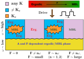
Figure 1: A schematic diagram of the different phases based on the average level spacing ratio. Top bar pertains to the undriven model ($\mathcal{F}(t)=F$). For the driven model, the different possibilities of the ergodic and MBL phases are also marked depending on the tuning of the parameters $K=A/\omega$ and $F$. In the high frequency, an MBL phase is obtained either by tuning the tuning the parameter at DL point or by off-resonant drive at strong field strengths. In the low frequency regime, the possibility of the ergodic and the MBL phase depends on the parameters $F$ and $A$. The actual transition from low-to-high frequency also depends on the different parameters of the system and hence shown by a wiggly line (only schematic in nature). The whole schematic is drawn while considering $K=A/\omega$ to lie below the second DL point.

An important open question has to do with the effect of a drive on a clean MBL system, which we address here. Specifically, we study the model resulting from the application of an ac field comprising of square wave pulses onto the clean MBL system of Schulz et al Schulz et al. (2019). Remarkably, the drive is found to take the undriven system from an ergodic phase to an MBL phase and vice-versa when the parameters are set appropriately. In the non-interacting limit, for the case of a combined dc and square-wave driving, we obtain analytically the conditions for dynamic localization (DL), coherent destruction of WS localization and super-Bloch oscillations.

Our main findings are captured schematically in Fig. 1. Keeping the dc field alone is equivalent to the undriven model, which exhibits a phase transition from an ergodic to a Stark MBL phase Schulz et al. (2019). In the presence of a high-frequency drive, we obtain an intricate set of possibilities dependent on how the static electric field and the ratio of the amplitude to the frequency ($A/\omega$) of the drive are tuned. The addition of a drive in the zero dc field limit, induces an MBL phase if the ratio $A/\omega$ is tuned close to the dynamic localization point, analogous to the drive-induced MBL phase reported Bairey et al. (2017) in a conventional disordered MBL model. For a large dc field, where the undriven model yields the Stark MBL phase, the addition of resonantly tuned drive leads to a destruction of Stark MBL for all values of the ratio $A/\omega$ tuned away from the dynamic localization point. We refer to this as coherent destruction of Stark-MBL. However, Stark MBL is found to be robust against off-resonant drive. Importantly, the coherent destruction of Stark-MBL is accompanied by the appearance of a large prethermal window before the final infinite-temperature-like state is reached, as captured by the dynamics of entanglement entropy. In the low-frequency limit, the nature of the phase obtained depends heavily on the choice of $F$ and $A$.

II Model Hamiltonian

The Hamiltonian of the system can be written as

$$H=-J\sum_{j=0}^{L-2}(c_{j}^{\dagger}c_{j+1}+c_{j+1}^{\dagger}c_{j})-\mathcal{F}(t)\sum_{j=0}^{L-1}j(n_{j}-\frac{1}{2})\qquad$$

$$+\alpha\sum_{j=0}^{L-1}\frac{j^{2}}{(L-1)^{2}}(n_{j}-\frac{1}{2})+V\sum_{j=0}^{L-2}(n_{j}-\frac{1}{2})(n_{j+1}-\frac{1}{2}),$$

where $V$ is the nearest neighbor interaction and $\mathcal{F}(t)=F+A\;\text{sgn}(\sin(\omega t))$ is a combined dc and ac electric field, with $A$ and $\omega$ respectively being the amplitude and frequency of the ac field ($F_{ac}$), while $F$ is the dc field. The curvature term (with strength $\alpha$) provides a non-linearity to the dc field and thus makes Stark-MBL possible Schulz et al. (2019). The lattice constant is kept at unity and natural units ($\hbar=e=1$) are adopted for all the calculations.

III Non-interacting case: Semi-classical description

Let us consider the non-interacting case ($V=0$), and with zero curvature $(\alpha=0)$. The quasi-momentum can be expressed as

$$q_{k}(t)=k+Ft+\int_{0}^{t}d\tau F_{ac}(\tau).$$ (2)

Due to the dc part, the quasi-momentum is no longer a periodic function. However, for the resonance condition $F=n\omega$, the quasi-momentum becomes a periodic function. Solving (as described in appendix A) for the one cycle average of quasi-energy, we get

$$\epsilon(k)=-2J_{\text{eff}}\cos(k+\frac{n\pi}{2}),$$ (3)

where

$$J_{\text{eff}}=J\left\{\frac{\sin(\frac{K\pi}{2}+\frac{n\pi}{2})}{(K\pi+n\pi)}+(-1)^{n}\frac{\sin(\frac{K\pi}{2}-\frac{n\pi}{2})}{(K\pi-n\pi)}\right\},$$ (4)

and $K=A/\omega$. In the limit $F=0$, this reduces to the well known quasi-energy dispersion for square wave driving: $\epsilon(k)=-2J\text{sinc}\left(\frac{\pi K}{2}\right)\cos k$, where $\text{sinc}(z)=\sin(z)/z$. The quasi-energy band collapses at the zeros of the function $\text{sinc}(\pi K/2)$, which occurs at $K=K_{c}=2\nu$, $\nu\in\mathbb{Z}$, which is the condition for dynamic localization  Eckardt et al. (2009).

For a finite $F=n\omega$, the quasi-energy spectrum can be further simplified. For even and odd $n$ respectively, we get $\epsilon(k)=-2J_{even}\cos k$ and $\epsilon(k)=-2J_{odd}\sin k$, where

$$J_{even}=\frac{2JK\sin(\frac{K\pi}{2})}{(K^{2}-n^{2})\pi};\;\;J_{odd}=\frac{2JK\cos(\frac{K\pi}{2})}{(K^{2}-n^{2})\pi}.$$ (5)

In the even and odd cases respectively, the band collapse occurs at $K=K_{c}=2\nu$ and $K=K_{c}=2\nu+1$, $\nu\in\mathbb{Z}$ and $K_{c}\neq n$. At these points an initially localized wave packet returns to its starting position. This gives the condition of dynamic localization. For other values of $K$, and provided that the resonance condition holds, band formation takes place and the WS localization due to the static dc field is destroyed. A slight detuning from resonance ($F=(n+\delta)\omega$), results in super-Bloch oscillations with the time period given by $T_{\text{SBO}}=\frac{2\pi}{\omega\delta}$ (Kudo and Monteiro, 2011; Longhi and Della Valle, 2012; Caetano and Lyra, 2011).

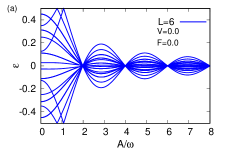
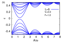
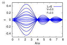
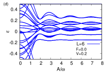
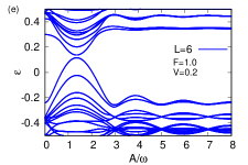
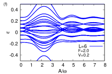
Figure 2: Top panel: Quasi-energy spectrum in the non-interacting case for different strengths of the static field. (a) for $F=0.0$, DL occurs for an even integer value of $A/\omega$. (b,c) DL for a finite value of the static field $F=n\omega$. The corresponding condition for DL also changes depending whether $n$ is odd (b) or even (c). Bottom panel: Quasi-energy spectrum for the interacting case with different strengths of the static field. A finite interaction avoids the band collapse thus destabilizing DL in the presence of interactions. The other parameters are: $L=6,\omega=1.0,t=0.25\ \text{and filling factor =}0.5$ in all the figures.

The band collapses for zero static field and both even and odd $n$ are shown in Fig. 2(a-c). The band collapse in Fig. 2(b) comes about because the quasi-energy is conserved modulo $\omega$, and therefore the zero level is the same as $0.5$.

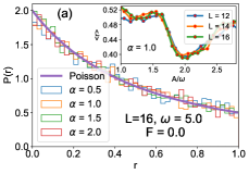
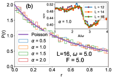
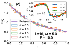
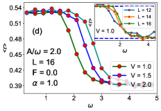
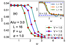
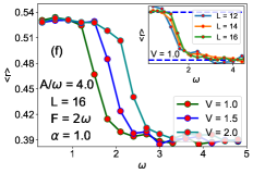
Figure 3: (a-c) Probability distribution of the quasi-energy gap ratio parameter for a high frequency drive ($\omega=5.0$) at the DL point. The cases $(a)$ without any dc field, $(b)$ resonantly tuned drive ($F=n\omega$) with $n$-odd and $(c)$ with $n$-even, are shown. The insets in (a-c) shows the average level-spacing ratio as a function of the ratio $A/\omega$ for different system sizes. (d-f) Frequency dependence of the average level-spacing ratio for various interaction strengths. In all the cases, the ratio $A/\omega$ is tuned at the DL point. (d) For zero dc field case, (e,f) For resonant drive with (e) $n$ odd and (f) $n$ even. The insets in (d-f) show the finite-size scaling of the frequency dependence transition for $\alpha=1.0$. The other parameters are: $J=1.0,V=1.0$.

IV Interacting model

In this section, we discuss how the presence of many-body interactions affect the dynamic localization and how the MBL phase can be obtained by including the curvature term.

IV.1 Absence of dynamic localization

For any general time-periodic Hamiltonian, the Floquet operator over one cycle can be expressed in terms of Floquet Hamiltonian $H_{F}$ as: $U(T)=\mathcal{T}\int_{0}^{T}e^{-iH(t)}dt=e^{-iH_{F}T}$, where $\mathcal{T}$ represents the time ordering and $T$ is the time period of the drive. For the square wave drive, defining $H_{+}$ and $H_{-}$ as the Hamiltonians for the first and second half of the driving period respectively, the Floquet operator can be simplified to $U(T)=(e^{-iH_{-}T/2}e^{-iH_{+}T/2})$. The required quasi-energies and the Floquet eigenstates are then calculated by numerically diagonalizing the Floquet operator (upto $L=16$ at half-filling).

The obtained quasi-energy spectrum for the interacting case with $\alpha=0$, is plotted in Fig. 2(d-f). We observe that the quasi-energy spectrum for all the cases of $F=0$,$\ n$-odd, and $n$-even, has a tendency to avoid the band collapse in contrast to the non-interacting problem (Fig. 2(a-c)) where the band does collapse at certain special points. This signifies the destruction of dynamic localization in the presence of many-body interactions.

IV.2 MBL in the presence of a curvature term

Although interactions are inimical to dynamic localization, the presence of a non-zero curvature term can lead to the MBL phase. As evident from the non-interacting case with $\alpha=0$, the drive re-normalizes the hopping strength (Eq. 5) and in the high-frequency limit, the Hamiltonian can be effectively written as a nearest-neighbor hopping model with re-normalized hopping strength for resonant driving. In the presence of interactions this picture fails as the quasi-momentum is no longer conserved. Nevertheless, there will be some residual suppression of the hopping strength  Luitz et al. (2017); Bairey et al. (2017). With only interactions, and tuning the parameters at the dynamic localization point ($J_{\text{eff}}=0$), this leads to the destruction of dynamic localization Luitz et al. (2017) and this eventually leads to a de-localization effect, however we point out that an additional non-zero onsite potential (curvature term) yields MBL around the dynamic localization point.

IV.2.1 High-frequency driving

To characterize the MBL phase, we study the probability distribution of the level spacing. Fig. 3 shows the probability distribution of the quasi-energy gap-ratio parameter: $r_{n}=\text{min}(\delta_{n}/\delta_{n+1},\delta_{n+1}/\delta_{n})$, where $\delta_{n}$ is the difference between the $n^{th}$ and $(n-1)^{th}$ quasi-energy levels, for a system of size $L=16$ and various values of the curvature term for a large driving frequency $\omega=5$. For all the cases $(F=0,n\omega)$, the probability distribution agrees with the Poisson distribution: $P(r)=2/(1+r)^{2}$ and suggests an MBL phase at these special points. The inset in Fig. 3(a) shows the level-spacing ratio as a function of $A/\omega$ for zero dc field. Although the un-driven model $F=0$, is in the ergodic phase Schulz et al. (2019), the application of drive leads to the MBL phase with a proper tuning of the ratio $A/\omega$ to the dynamic localization point ($A/\omega=2\nu$ with $\nu\in\mathbb{Z}$) of the non-interacting problem.

For the case where an additional static field is also present and satisfies the resonance condition: $F=n\omega$, the condition for dynamic localization in the non-interacting limit depends on whether the integer $n$ is odd or even (Eq. 5). We therefore explore both the cases setting $F=5,10$ (corresponding to $n=1,2$ respectively) as shown in the insets of the Fig. 3(b,c). The un-driven model corresponding to these field strengths shows the Stark-MBL phase. By turning on the drive in this case, we find that the Stark-MBL phase can be destroyed with resonant driving. We therefore term this phenomenon as “coherent destruction of Stark-MBL”. However, close to the points of dynamic localization, Stark-MBL is found to remain intact. Thus we see that by a proper tuning of $F$, $A$, and $\omega$ it is possible to convert the ergodic phase into the MBL phase and vice versa.

We have seen that tuning the ratio $A/\omega$ at the dynamic localization point, seems to favour MBL. However, this turns out to be true only for sufficiently high frequencies, and in fact, there is a frequency-dependent transition from the ergodic to the MBL phase. To demonstrate this, we tune the ratio $A/\omega$ at the dynamic localization point and vary the driving frequency $\omega$, while keeping the ratio $A/\omega$ fixed. For the zero static field case, Fig 3 (d) shows the average level spacing for various interaction strengths. Fig 3 (e) and Fig 3 (f) consider the scenario when an additional dc field is present. Here, in addition to keeping the ratio $A/\omega$ fixed at the dynamic localization point, we also keep the ratio $F/\omega$ fixed (at $1$,$2$ respectively) as $\omega$ is varied. It can be seen that only at sufficiently high frequency an MBL phase is observed. Moreover, the frequency required to observe the MBL phase also increases on increasing the interaction strength. This can be understood from the phase diagram of the undriven system (see appendix B), where the ergodic-to-MBL phase transition occurs at a higher value of the field strength on increasing the interaction strength. In the presence of the drive, an MBL phase is obtained only when the effective field in the two half-cycles ($F\pm A$) lies in the deep-MBL region of the undriven system where the drive only mixes the localized states of the undriven system. The insets of Fig 3 (d-f) show the finite-size scaling for $V=1.0$ and supports the argument presented above.

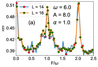
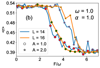
Figure 4: (a) High Frequency drive: Average level-spacing ratio as a function of $F/\omega$ and away from the DL point ($\omega=6.0,A=8.0$). For the condition $F=n\omega$, Stark-MBL is destroyed while for off-resonant driving, the Stark-MBL phase is robust. (b) Low frequency drive: The average level spacing ratio as a function of $F/\omega$ for $A=1.0,2.0$ for $(\omega=1.0)$. The transition from ergodic to the MBL phase is found to be dependent on the parameters $A$ and $F$. The other parameters are: $J=1.0,V=1.0$, and $\alpha=1.0$

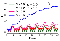
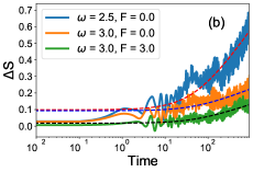
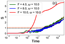
Figure 5: (a) Absence of DL in the presence of many-body interactions (with $\alpha=0$). A departure from perfect periodicity is observed. (b) Dynamics of the difference in EE ($\Delta S$) between the interacting and the corresponding non-interacting limit, at the DL point. The plots are smoothed out by convolution with a Gaussian: $w(n)=e^{-(n/\sigma)^{2}/2}$, with $\sigma=5$. (c) Coherent destruction of Stark-MBL phase at resonant driving and the robustness of Stark-MBL phase at off-resonant driving from the EE dynamics. The fitting is done with the curve: $f(x)=a\log(x)+b$. The other parameters are: $L=18,J=1.0,V=1.0,\alpha=1.0$.

Finally, we consider the case of an off-resonant drive. Fig. 4(a) shows the level-spacing ratio as a function of the ratio $F/\omega$. Only when the ratio $F/\omega$ approaches an integer, the level spacing ratio satisfies the Wigner-Dyson statistics signifying an ergodic phase for these special ratios. Thus, we see that in the high-frequency regime, Stark-MBL remains robust against off-resonant drive.

IV.2.2 Low-frequency driving

In the low-frequency regime, the nature of the phase crucially depends on the choice of the driving amplitude and the static field strength. Fig. 4(b) shows the variation of the average level spacing ratio as a function of the static dc field for different driving amplitudes. It can be seen that the ergodic-to-MBL phase transition depends on the choice of driving amplitude. The driven model yields an MBL phase when both $F+A$ and $F-A$ lie in the MBL phase of the undriven model, where the drive only mixes the localized eigenstates of the undriven system. On the other hand, when one or both of the parameters: $F+A$ or $F-A$ falls into the ergodic region of the undriven model, an ergodic phase is observed. We infer that if the drive mixes both localized and extended states, it is extended states that dominate.

V Dynamics of entanglement entropy

For a system in a pure state, the entanglement entropy (EE) of a subsystem $A$ is defined as: $S_{A}=-\text{Tr}(\rho_{A}\text{ln}\rho_{A})$, where $\rho_{A}$ is the reduced density matrix of the subsystem $A$ obtained by tracing out the degrees of freedom of the other subsystem $B$. To study the dynamics of the entanglement entropy, we start with an initial product state (where all the particles occupy the even sites) and use an exact numerical approach based on the re-orthogonalized Lanczos algorithm van Nieuwenburg et al. (2019); Luitz and Lev (2017) for the time evolution. Due to the interactions in the MBL phase, a logarithmic growth of the entanglement entropy is expected (Žnidarič et al., 2008; Bardarson et al., 2012; Serbyn et al., 2013).

We first consider the limit $\alpha=0$, and study the stability of dynamic localization in the presence of interactions. The dynamics of entanglement entropy for various interaction strengths is plotted in Fig. 5(a), where the ratio $A/\omega$ is tuned at the dynamic localization point. The entanglement entropy here starts to grow in time as opposed to the non-interacting case where as a consequence of the band collapse, it shows an oscillatory behavior and recurs to its initial value state) at times $t=mT$ with $m$ being a positive integer.

We now turn to the case with a finite curvature strength ($\alpha=1.0$), where an MBL phase is found at sufficiently high frequencies.We first consider the case where the MBL phase is obtained by tuning the ratio $A/\omega$ at the dynamic localization point. We define the quantity: $\Delta S=S(t,V)-S(t,V=0)$ as the difference between the entanglement entropy of the interacting and the corresponding non-interacting limit. Fig. 5(b) shows the dynamics of $\Delta S$ as a function of time for different sets of the frequency and the static field. In all the cases, a logarithmic behavior is observed which signifies an MBL-like phase at these points.

The dynamics of the entanglement entropy for the parameters tuned away from the dynamic localization point is shown in Fig. 5(c). It can be seen that for resonant drive ($F=n\omega$), the Stark-MBL phase is destroyed. The entanglement entropy increases rapidly for smaller times followed by a slow growth for the intermediate times and finally saturates to its thermal value. This slow growth of entanglement entropy in the intermediate times is a signature of Floquet prethermalization (Abanin et al., 2017a; Mori et al., 2016; Abanin et al., 2017b; Luitz et al., 2019), where the system prethermalizes before reaching an infinite-temperature-like state at high frequencies. For the off-resonant drive at high frequency, the entanglement entropy shows the usual logarithmic growth signifying the robustness of the Stark-MBL phase.

VI Summary and Conclusions

. To summarize, we study a clean interacting system driven by a combined ac and dc electric field. The underlying non-interacting problem is itself of interest, and we semi-classically obtain the condition for dynamic localization, coherent destruction of WS localization and super Bloch oscillations. In the presence of interactions, generic clean many-body systems under a drive, reach a featureless infinite-temperature-like state. In contrast, we find that our system can avoid such ‘heat death’, under high-frequency drive. This is achieved either by tuning the system at the dynamic localization point of the corresponding noninteracting model, or by subjecting the system to off-resonant drive.

We further study the fate of the Stark-MBL phase in the presence of an additional drive. Observing that the effects of low-frequency driving are heavily dependent on the field strength and the amplitude of the drive, we focus on high-frequency driving, uncovering an intricate set of possible phases. One striking possibility is that of generating an MBL phase from the undriven ergodic phase by the application of a pure ac field. A second remarkable possibility appears for sufficiently large dc field, where it is possible to destroy Stark-MBL, by the application of a resonantly tuned drive provided that the ratio $A/\omega$ is tuned away from the dynamic localization point. We term this as ‘coherent destruction of Stark-MBL’. On the other hand, the Stark-MBL phase is found to be robust against off-resonant drive.

Appendix A Non- interacting Case: Semi-classical Description

The form of the combined dc and ac field can be written as

$$\mathcal{F}(t)=\begin{cases}F+A&\text{for }0\leq t<T/2\\ F-A&\text{for }T/2\leq t<T,\\ \end{cases}$$ (6)

where $A$ and $T$ are the amplitude and the time-period of the drive respectively and $F$ is the static field strength.

Firstly, we will consider the case where the static field is absent ($F=0$). The quasi-momentum in the presence of this time dependent field changes as:$q_{k}(t)=k+\frac{1}{\hbar}\int_{0}^{t}d\tau\mathcal{F}(\tau).$ For square wave driving (Eq. 6), the expression for the quasi-momentum can be solved as Eckardt et al. (2009):

$$q_{k}(t)=\begin{cases}k+A(t-T/4)/\hbar&\text{for }0\leq t<T/2\\ k+A(3T/4-t)/\hbar&\text{for }T/2\leq t<T.\\ \end{cases}$$ (7)

The change in the quasi-momentum leads to a change in the dispersion, which is now time-dependent ($E(k)=-2J\cos(q_{k}(t))$). Due to the absence of energy conservation, we focus on the one-cycle average of the quasi-energy, which is given by: $\epsilon(k)=\frac{-2J}{T}\int_{0}^{T}\cos[q_{k}(t)]\ dt.$ Substituting the expression for $q_{k}(t)$ and solving the integral, we get

$$\epsilon(k)=-2J\text{sinc}\left(\frac{\pi K}{2}\right)\cos(k),$$ (8)

where, $\text{sinc}(z)=\sin(z)/z$ and $K=A/\omega$. The quasi-energy band collapses at the zeros of the function $\text{sinc}(\pi K/2)$, which occurs when $K=K_{c}=2\nu$, $\nu$ being any integer (Fig. 2(a)). This is the condition for dynamic localization.

For a combined ac and dc field the quasi-momentum can be expressed as: $q_{k}(t)=k+Ft+\int_{0}^{t}d\tau F_{ac}(\tau)$

Due to the dc part, the quasi-momentum is no longer a periodic function. However, for the resonance condition $F=n\omega$, the quasi-momentum becomes a periodic function. Solving for the one cycle average of quasi-energy, we get

$$\epsilon(k)=\frac{-2J}{T}\int_{0}^{T}\cos[q_{k}(t)]\ dt=\frac{-2J}{T}\int_{0}^{T/2}\cos\left(k+n\omega t+A(t-T/4)\right)\ dt+\int_{T/2}^{T}\cos\left(k+n\omega t+A(3T/4-t)\right)\ dt.$$ (9)

The integral can be solved to yield:

$$\epsilon(k)=-2J_{\text{eff}}\cos(k+\frac{n\pi}{2}),\ \ \text{and}\quad J_{\text{eff}}=J\left\{\frac{\sin(\frac{n\pi}{2}+\frac{K\pi}{2})}{(K\pi+n\pi)}+(-1)^{n}\frac{\sin(-\frac{n\pi}{2}+\frac{K\pi}{2})}{(K\pi-n\pi)}\right\}$$ (10)

A.1 Case 1: Odd $n$

For odd $n$, Eqn. 10 can be simplified to

$$\epsilon(k)=-2J\left(\frac{2K\cos(\frac{K\pi}{2})}{(K^{2}-n^{2})\pi}\right)\cos(k-\frac{\pi}{2}).$$ (11)

Here, the band collapses for $K=K_{c}=2\nu+1,\ \nu\in\mathbb{Z}$ and $K_{c}\neq n$ (Fig. 2(b)). This gives the condition of dynamic localization whereas for other $K$ with the resonance condition destruction of Wannier-Stark localization occurs.

A.2 Case 2: Even $n$

For even $n$, Eqn. 10 can be simplified to

$$\epsilon(k)=-2J\left(\frac{2K\sin(\frac{K\pi}{2})}{(K^{2}-n^{2})\pi}\right)\cos(k)=-2J\left(\frac{\text{sinc}(\frac{K\pi}{2})}{1-\frac{n^{2}}{K^{2}}}\right)\cos(k).$$ (12)

Again, the band collapse occurs at $K=K_{c}=2\nu,\ \nu\in\mathbb{Z}$ and $K_{c}\neq n$ (Fig. 2(c)). At these points an initially localized wave packet returns to its starting position. This gives the condition of dynamical localization. For other values of $K$, and provided that the resonance condition holds, band formation takes place and the WS localization due to the static dc field is destroyed.

A.3 Super-Bloch Oscillations

Considering the case of a slight detuning from the resonant condition: $F=(n+\delta)\omega$, the corresponding quasi-momentum can be written as: $q_{k}(t)=k+n\omega t+\delta\omega t+\int_{0}^{t}d\tau F_{ac}(\tau)$. The quasi-momentum is no longer periodic due to the extra term. However for $\delta<<1$, we can approximately take $q_{k}(t)$ as periodic and can proceed further to calculate the quasi-energy by assuming $\delta\omega t$ as a constant. It can be easily verified that for both even and odd $n$, the cosine term $\cos(k)$, acquires an additional phase $\delta\omega t$, which is equivalent to a static dc field of magnitude $\delta\omega$. The dynamics shows oscillatory behaviour similar to Bloch oscillations. These oscillations are termed as super-Bloch oscillations. The time period is given by: $T_{\text{SBO}}=\frac{2\pi}{\delta\omega}$.

Appendix B Undriven system: $\mathcal{F}(t)=F$

In the absence of driving, the Hamiltonian can be written as

$$H=-J\sum_{j=0}^{L-2}(c_{j}^{\dagger}c_{j+1}+c_{j+1}^{\dagger}c_{j})-F\sum_{j=0}^{L-1}j(n_{j}-\frac{1}{2})+\alpha\sum_{j=0}^{L-1}\frac{j^{2}}{(L-1)^{2}}(n_{j}-\frac{1}{2})+V\sum_{j=0}^{L-2}(n_{j}-\frac{1}{2})(n_{j+1}-\frac{1}{2}).$$ (13)

The model shows an ergodic phase for small field strengths, while for sufficiently strong field strength it shows an MBL phase.

To study the different phases, we plot the average level-spacing ratio as a function of field strength (Fig. 6(a)). For small field strength the level-spacing follows Wigner-Dyson statistics while for large field strength it follows Poisson statistics signifying an MBL phase for these values of the field strength. Finally, we also look at the interplay of the interactions and the field strength. Fig. 6(b) shows the surface plot of the average level-spacing ratio as a function of both field strength and the interaction strength. On increasing the interaction strength, the field required to show MBL also increases.

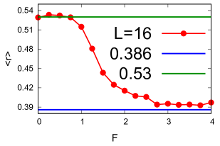
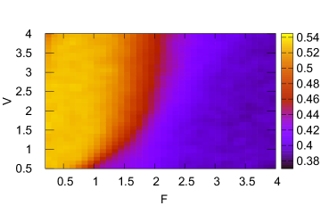
Figure 6: Left: Average level-spacing ratio as a function of the field strength for a fixed $V=1.0$. Right: Surface plot of the level statistics as a function of both field strength $(F)$ and the interaction strength $(V)$. The other parameters are: $L=16,\alpha=1.0$.

References

- Alet and Laflorencie (2018) F. Alet and N. Laflorencie, Comptes Rendus Physique 19, 498 (2018).
- Abanin and Papić (2017) D. A. Abanin and Z. Papić, Annalen der Physik 529, 1700169 (2017).
- Abanin et al. (2018) D. A. Abanin, E. Altman, I. Bloch, and M. Serbyn, arXiv preprint arXiv:1804.11065 (2018).
- Basko et al. (2006) D. M. Basko, I. L. Aleiner, and B. L. Altshuler, Annals of physics 321, 1126 (2006).
- Gornyi et al. (2005) I. V. Gornyi, A. D. Mirlin, and D. G. Polyakov, Phys. Rev. Lett. 95, 206603 (2005).
- Nandkishore and Huse (2015) R. Nandkishore and D. A. Huse, Annu. Rev. Condens. Matter Phys. 6, 15 (2015).
- Anderson (1958) P. W. Anderson, Phys. Rev. 109, 1492 (1958).
- Schulz et al. (2019) M. Schulz, C. Hooley, R. Moessner, and F. Pollmann, Physical review letters 122, 040606 (2019).
- van Nieuwenburg et al. (2019) E. van Nieuwenburg, Y. Baum, and G. Refael, Proceedings of the National Academy of Sciences , 201819316 (2019).
- Bhakuni and Sharma (2019) D. S. Bhakuni and A. Sharma, arXiv preprint arXiv:1909.10542 (2019).
- Taylor et al. (2019) S. R. Taylor, M. Schulz, F. Pollmann, and R. Moessner, arXiv preprint arXiv:1910.01154 (2019).
- Abanin et al. (2015) D. A. Abanin, W. De Roeck, and F. Huveneers, Physical review letters 115, 256803 (2015).
- D’Alessio and Rigol (2014) L. D’Alessio and M. Rigol, Physical Review X 4, 041048 (2014).
- Lazarides et al. (2014a) A. Lazarides, A. Das, and R. Moessner, Physical Review E 90, 012110 (2014a).
- Lazarides et al. (2014b) A. Lazarides, A. Das, and R. Moessner, Physical review letters 112, 150401 (2014b).
- Ray et al. (2018a) S. Ray, A. Ghosh, and S. Sinha, Physical Review E 97, 010101 (2018a).
- Ray et al. (2018b) S. Ray, S. Sinha, and K. Sengupta, Physical Review A 98, 053631 (2018b).
- Abanin et al. (2017a) D. A. Abanin, W. De Roeck, W. W. Ho, and F. Huveneers, Physical Review B 95, 014112 (2017a).
- Weidinger and Knap (2017) S. A. Weidinger and M. Knap, Scientific reports 7, 1 (2017).
- Gómez-León and Platero (2013) A. Gómez-León and G. Platero, Phys. Rev. Lett. 110, 200403 (2013).
- Cayssol et al. (2013) J. Cayssol, B. Dóra, F. Simon, and R. Moessner, physica status solidi (RRL)–Rapid Research Letters 7, 101 (2013).
- Rudner et al. (2013) M. S. Rudner, N. H. Lindner, E. Berg, and M. Levin, Physical Review X 3, 031005 (2013).
- Else et al. (2016) D. V. Else, B. Bauer, and C. Nayak, Physical review letters 117, 090402 (2016).
- Ponte et al. (2015a) P. Ponte, A. Chandran, Z. Papić, and D. A. Abanin, Annals of Physics 353, 196 (2015a).
- Lazarides et al. (2015) A. Lazarides, A. Das, and R. Moessner, Physical review letters 115, 030402 (2015).
- Abanin et al. (2016) D. A. Abanin, W. De Roeck, and F. Huveneers, Annals of Physics 372, 1 (2016).
- D’Alessio and Polkovnikov (2013) L. D’Alessio and A. Polkovnikov, Annals of Physics 333, 19 (2013).
- Ponte et al. (2015b) P. Ponte, Z. Papić, F. Huveneers, and D. A. Abanin, Physical review letters 114, 140401 (2015b).
- Bordia et al. (2017) P. Bordia, H. Lüschen, U. Schneider, M. Knap, and I. Bloch, Nature Physics 13, 460 (2017).
- Singh et al. (2019) K. Singh, C. J. Fujiwara, Z. A. Geiger, E. Q. Simmons, M. Lipatov, A. Cao, P. Dotti, S. V. Rajagopal, R. Senaratne, T. Shimasaki, et al., Physical Review X 9, 041021 (2019).
- Rubio-Abadal et al. (2020) A. Rubio-Abadal, M. Ippoliti, S. Hollerith, D. Wei, J. Rui, S. Sondhi, V. Khemani, C. Gross, and I. Bloch, arXiv preprint arXiv:2001.08226 (2020).
- Dunlap and Kenkre (1986) D. Dunlap and V. Kenkre, Physical Review B 34, 3625 (1986).
- Dunlap and Kenkre (1988) D. Dunlap and V. Kenkre, Physics Letters A 127, 438 (1988).
- Bhakuni and Sharma (2018) D. S. Bhakuni and A. Sharma, Phys. Rev. B 98, 045408 (2018).
- Eckardt et al. (2009) A. Eckardt, M. Holthaus, H. Lignier, A. Zenesini, D. Ciampini, O. Morsch, and E. Arimondo, Physical Review A 79, 013611 (2009).
- Bairey et al. (2017) E. Bairey, G. Refael, and N. H. Lindner, Physical Review B 96, 020201 (2017).
- Holthaus et al. (1995a) M. Holthaus, G. Ristow, and D. Hone, EPL (Europhysics Letters) 32, 241 (1995a).
- Holthaus et al. (1995b) M. Holthaus, G. H. Ristow, and D. W. Hone, Physical review letters 75, 3914 (1995b).
- Bhakuni et al. (2019) D. S. Bhakuni, S. Dattagupta, and A. Sharma, Phys. Rev. B 99, 155149 (2019).
- Kudo and Monteiro (2011) K. Kudo and T. Monteiro, Physical Review A 83, 053627 (2011).
- Longhi and Della Valle (2012) S. Longhi and G. Della Valle, Phys. Rev. B 86, 075143 (2012).
- Caetano and Lyra (2011) R. Caetano and M. Lyra, Physics Letters A 375, 2770 (2011).
- Luitz et al. (2017) D. J. Luitz, Y. Bar Lev, and A. Lazarides, SciPost Physics 3, 029 (2017).
- Luitz and Lev (2017) D. J. Luitz and Y. B. Lev, Annalen der Physik 529, 1600350 (2017).
- Žnidarič et al. (2008) M. Žnidarič, T. Prosen, and P. Prelovšek, Physical Review B 77, 064426 (2008).
- Bardarson et al. (2012) J. H. Bardarson, F. Pollmann, and J. E. Moore, Phys. Rev. Lett. 109, 017202 (2012).
- Serbyn et al. (2013) M. Serbyn, Z. Papić, and D. A. Abanin, Phys. Rev. Lett. 110, 260601 (2013).
- Mori et al. (2016) T. Mori, T. Kuwahara, and K. Saito, Physical review letters 116, 120401 (2016).
- Abanin et al. (2017b) D. Abanin, W. De Roeck, W. W. Ho, and F. Huveneers, Communications in Mathematical Physics 354, 809 (2017b).
- Luitz et al. (2019) D. J. Luitz, R. Moessner, S. Sondhi, and V. Khemani, arXiv preprint arXiv:1908.10371 (2019).