Zeroth-order Stochastic Compositional Algorithms for Risk-Aware Learning

Abstract

We present $\textit{Free-MESSAGE}^{p}$, the first zeroth-order algorithm for (weakly-)convex mean-semideviation-based risk-aware learning, which is also the first three-level zeroth-order compositional stochastic optimization algorithm whatsoever. Using a non-trivial extension of Nesterov’s classical results on Gaussian smoothing, we develop the $\textit{Free-MESSAGE}^{p}$ algorithm from first principles, and show that it essentially solves a smoothed surrogate to the original problem, the former being a uniform approximation of the latter, in a useful, convenient sense. We then present a complete analysis of the $\textit{Free-MESSAGE}^{p}$ algorithm, which establishes convergence in a user-tunable neighborhood of the optimal solutions of the original problem for convex costs, as well as explicit convergence rates for convex, weakly convex, and strongly convex costs, and in a unified way. Orderwise, and for fixed problem parameters, our results demonstrate no sacrifice in convergence speed as compared to existing first-order methods, while striking a certain balance among the condition of the problem, its dimensionality, as well as the accuracy of the obtained results, naturally extending previous results in zeroth-order risk-neutral learning.

90-08, 90C25, 90C15, 90C59, 90C99

1 Introduction

Statistical machine learning traditionally deals with the determination and characterization of optimal decision rules minimizing an expected cost criterion, quantifying, for instance, regression or misclassification error in relevant applications, on the basis of available training data [17, 20, 43]. Still, the expected cost paradigm is not appropriate, say, in applications involving highly dispersive disturbances, such as heavy tailed, skewed or multimodal noise, or in applications whose purpose is to imitate uncertain human behavior. In the first case, merely optimizing the expected cost is often statistically meaningless, since the resulting optimal prediction errors might exhibit unstable or erratic behavior, even with a small expected value. In the second case, as aptly put in [7], the fact is that human decision makers are inherently risk-averse, because they prefer consistent sequences of predictions instead of highly variable ones, even if the latter contain slightly better predictions.

Such situations motivate developments in the area of risk-aware statistical learning, in which expectation in the learning objective is replaced by more general functionals, called risk measures [39], whose purpose is to effectively quantify the statistical variability of the cost function considered, in addition to mean performance. Indeed, risk-awareness in learning and optimization has already been explored under various problem settings [1, 5, 7, 18, 21, 22, 23, 26, 31, 37, 41, 44, 47, 49], and has proved useful in many important applications, as well [5, 6, 24, 27, 34, 38].

In this paper, we study risk-aware learning problems in which expectation is generalized to the class of mean-semideviation risk measures developed in [23]. Specifically, given any complete probability space $\left(\Omega,\mathscr{F},{\cal P}\right)$, and a random element $\boldsymbol{W}:\Omega\rightarrow\mathbb{R}^{M}$ on $\left(\Omega,\mathscr{F}\right)$ modeling abstractly all the uncertainty involved in the learning task, we consider stochastic programs of the form

(1) $$\underset{\boldsymbol{x}\in{\cal X}}{\inf}\>\big{\{}\phi\left(\boldsymbol{x}\right)\triangleq\mathbb{E}\left\{F\left(\boldsymbol{x},\boldsymbol{W}\right)\right\}+c\left\|{\cal R}\left(F\left(\boldsymbol{x},\boldsymbol{W}\right)-\mathbb{E}\left\{F\left(\boldsymbol{x},\boldsymbol{W}\right)\right\}\right)\right\|_{{\cal L}_{p}}\big{\}},$$

for $c\in[0,1]$ and order $p\in\left[1,2\right]$, and where $F:\mathbb{R}^{N}\times\mathbb{R}^{M}\rightarrow\mathbb{R}$ is Borel in its second argument and either weakly convex, convex, or strongly convex in its first, $F\left(\cdot,\boldsymbol{W}\right)\in{\cal L}_{p}\left(\Omega,\mathscr{F},{\cal P};\mathbb{R}\right)\triangleq{\cal Z}_{p}$ , $\|\cdot\|_{{\cal L}_{p}}:{\cal Z}_{p}\rightarrow\mathbb{R}_{+}$ is the corresponding standard norm on ${\cal Z}_{p}$, the set ${\cal X}\subseteq\mathbb{R}^{N}$ is nonempty, closed and convex, and ${\cal R}:\mathbb{R}\rightarrow\mathbb{R}$ is a risk regularizer, or risk profile [23], that is, any convex, nonnegative, nondecreasing and nonexpansive function. Hereafter, (1) will be called the base problem.

The objective $\phi$ evaluates the mean-semideviation risk measure $\rho\left(\cdot\right)\triangleq\mathbb{E}\left\{\cdot\right\}+c\|{\cal R}\left((\cdot)-\mathbb{E}\left\{\cdot\right\}\right)\|_{{\cal L}_{p}}$ at $F\left(\cdot,\boldsymbol{W}\right)$, i.e., $\phi\left(\cdot\right)\equiv\rho\left(F\left(\cdot,\boldsymbol{W}\right)\right)$ [23]. The functional $\rho$ generalizes the well-known mean-upper-semideviation [39], which is recovered by choosing ${\cal R}\left(\cdot\right)\equiv\left(\cdot\right)_{+}\triangleq\max\left\{\cdot,0\right\}$, and is one of the most popular risk-measures in theory and practice [2, 9, 14, 25, 32, 33, 35, 36]. For $c\in\left[0,1\right]$, $\rho$ is a convex risk measure [23], ([39], Section 6) on ${\cal Z}_{p}$; thus, whenever $F$ is convex, $\phi$ in (1) is convex on $\mathbb{R}^{N}$, as well.

In (1), the expected cost, called the risk-neutral part of the objective, is penalized by a semideviation term, called the risk-averse part of the objective. The latter explicitly quantifies, for each feasible decision, the deviation of the cost relative to its expectation, interpreted as a standardized statistical benchmark. The risk profile ${\cal R}$ acts on this central deviation as a weighting function, and its purpose is to reflect the particular risk preferences of the learner. As partially mentioned above, typical choices for ${\cal R}$ include the hockey stick $\left(\cdot\right)_{+}+\eta$, also known as a Rectified Linear Unit (ReLU), as well as its smooth approximations $(1/t)\log\left(1+\exp\left(t\left(\cdot\right)\right)\right)+\eta,$ with $t>0$, and $\eta\geq 0$. For a constructive characterization of mean-semideviation risk-measures, the reader is referred to [23].

Stochastic subgradient-based recursive optimization of mean-semideviation risk measures was recently considered in [23], where the so-called $\textit{MESSAGE}^{p}$ algorithm was proposed and analyzed for solving (1). The work of [23] is based on the fact that (1) can be expressed in nested form (see Section 2), and builds on previous results on general compositional stochastic optimization [45, 46].

In this work, we are interested in solving (1) in a zeroth-order setting, using exclusively cost function evaluations, in absence of gradient information. Zeroth-order methods have a long history in both deterministic and risk-neutral stochastic optimization [4, 12, 15, 16, 19, 29, 40, 48], and are of particular interest in applications where gradient information is very difficult, or even impossible to obtain, such as training of deep neural networks [8, 42], nonsmooth optimization [30], clinical trials [7], and, more generally, machine learning in the field, simulation-based optimization [10, 40], online auctions and search engines [12], and distributed learning [48]. Still, to the best of our knowledge, the development of zeroth-order methods for possibly nonsmooth risk-aware problems such as (1) and, more generally, compositional stochastic optimization problems, is completely unexplored. Our contributions are as follows:

• We present $\textit{Free-MESSAGE}^{p}$, the first zeroth-order algorithm for solving (1) within a user-specified accuracy, which is also the first three-level zeroth-order compositional stochastic optimization algorithm, whatsoever. The $\textit{Free-MESSAGE}^{p}$ algorithm requires exactly four cost function evaluations per iteration, and is based on finite difference-based inexact quasigradients, in the spirit of [15, 16, 30]. By using a non-trivial extension of Nesterov’s classical results on Gaussian smoothing [30], which we present and discuss (Section 3), we develop the $\textit{Free-MESSAGE}^{p}$ algorithm from first principles (Section 4), and we show that it essentially solves a smoothed surrogate to the original problem, the former provably being a uniform approximation to the latter (Lemma 5.1).

• We present a complete analysis of the $\textit{Free-MESSAGE}^{p}$ algorithm, establishing path convergence in a user-specified neighborhood of the optimal solutions of (1) for convex costs (Theorem 6.8), as well as explicit convergence rates for convex, weakly convex and strongly convex costs (Theorems 6.10, 6.12 and 6.14/6.16, respectively). Orderwise, and for fixed problem parameters, our results demonstrate no sacrifice in convergence speed as compared to the fully gradient-based $\textit{MESSAGE}^{p}$ algorithm [23], and explicitly quantify the effects of strong convexity on problem conditioning, reflected on the derived rates. Also, our results exhibit certain tradeoffs between the size of the limiting neighborhood and the decision dimension $N$, and naturally extend core prior work on zeroth-order risk-neutral optimization [30]. Lastly, our results are supported by indicative numerical simulations (Section 7).

As compared with prior works that assume access to stochastic gradients [23, 45, 46], passing to the zeroth-order setting is challenging for several reasons, on top of the corresponding convergence analysis (Section 6). First, the key fact that $\textit{Free-MESSAGE}^{p}$ can be designed in a way that it itself constitutes a stochastic gradient method tackling directly a well-defined and clearly identifiable smoothed surrogate to the original risk-aware problem is non-trivial (Section 5); this is because the objective $\phi$ in (1) does not admit an expectation representation, as otherwise standard in stochastic optimization. Of course, such a surrogate does not emerge in a gradient-based setting [23], at least as an essential entity.

At the same time, the connection between the smoothed surrogate and the original risk-aware problem is also not trivial: In fact, the analysis leading to our relevant uniform approximation bounds is substantially different from and more complex than that under the risk-neutral (expectation-based) setting [30], in regard to both the structure of our proofs (Lemma 5.1, Proposition 5.2), and the novel technical conditions imposed on the problem (Section 3, and Assumption 5). Those approximation bounds then make it possible to analyze convergence of $\textit{Free-MESSAGE}^{p}$ as a method for solving the smoothed surrogate, and subsequently relate the obtained results to the base problem (Section 6), in a transparent way. The corresponding analysis takes place under additional technical conditions (Assumption 6, which may be thought of as an evolution of Assumption 5, in turn following the discussion in Section 3), which are also new and different from those in [23, 45, 46].

Potentially Nonstandard Notation: We use bold letters to denote multidimensional quantities, such as vectors and matrices. Additionally, the symbol “$\triangleq$” denotes equality by definition, the symbol “$\equiv$” denotes immediate equality/equivalence, whereas the standard symbol “$=$” denotes possibly not immediate equality/equivalence. For a general vector/matrix-valued function $\boldsymbol{f}\in{\cal F}$, the graph of $\boldsymbol{f}$ on a set ${\cal G}$ is defined as the set $\mathrm{Graph}_{{\cal G}}\left(\boldsymbol{f}\right)\triangleq\{(\boldsymbol{x},\boldsymbol{y})\in{\cal G}\times{\cal F}\hskip 1.00374pt|\hskip 1.00374pt\boldsymbol{y}=\boldsymbol{f}(\boldsymbol{x})\}$. Lastly, within a given Cartesian product space, tuples are referred to as $(\boldsymbol{x},\boldsymbol{y},\boldsymbol{z},\ldots)$ or, in vector format, $[\boldsymbol{x}|\boldsymbol{y}|\boldsymbol{z}|\ldots]$.

2 Basic Properties of the Base Problem

First, it will be convenient to express $\phi$ in compositional (or nested) form, as in [23]. By defining expectation functions $\varrho:\mathbb{R}_{+}\rightarrow\mathbb{R}$, $g:\mathbb{R}^{N}\times\mathbb{R}\rightarrow\mathbb{R}_{+}$, $\boldsymbol{h}:\mathbb{R}^{N}\rightarrow\mathbb{R}^{N}\times\mathbb{R}$ and $s:\mathbb{R}^{N}\rightarrow\mathbb{R}$ as

$$\varrho\left(x\right)\triangleq x^{1/p},\;g\left(\boldsymbol{x},y\right)\triangleq\mathbb{E}\left\{\left({\cal R}\left(F\left(\boldsymbol{x},\boldsymbol{W}\right)-y\right)\right)^{p}\right\},\;\boldsymbol{h}\left(\boldsymbol{x}\right)\triangleq[\boldsymbol{x}\,|\,s\left(\boldsymbol{x}\right)\triangleq\mathbb{E}\left\{F\left(\boldsymbol{x},\boldsymbol{W}\right)\right\}],$$

respectively, and provided that the involved quantities are well-defined, $\phi$ may be reexpressed as

$$\phi\left(\boldsymbol{x}\right)\equiv s\left(\boldsymbol{x}\right)+c\varrho\left(g\left(\boldsymbol{h}\left(\boldsymbol{x}\right)\right)\right),\quad\forall\boldsymbol{x}\in{\cal X}.$$

Further, under appropriate conditions, differentiability of $\phi$ may be ensured as follows.

Lemma 2.1 (Differentiability of $\phi$ [23]).

Let $s$ and $g$ be differentiable on ${\cal X}$ and $\mathrm{Graph}_{{\cal X}}\left(s\right)$, respectively, and let ${\cal R}:\mathbb{R}\rightarrow\mathbb{R}$ be such that $\left\{x\in\mathbb{R}\left|{\cal R}\left(x\right)\equiv 0\right.\right\}\neq\mathbb{R}$. Also, if $p\in\left(1,2\right]$, and with $\kappa_{{\cal R}}\triangleq\sup\left\{x\in\mathbb{R}\left|{\cal R}\left(x\right)\equiv 0\right.\right\}\in\left[-\infty,\infty\right)$, suppose that ${\cal P}\left(F\left(\boldsymbol{x},\boldsymbol{W}\right)-s\left(\boldsymbol{x}\right)\leq\kappa_{{\cal R}}\right)<1$, for all $\boldsymbol{x}\in{\cal X}$. Then $\phi$ is differentiable on ${\cal X}$, and its gradient $\nabla\phi:\mathbb{R}^{N}\rightarrow\mathbb{R}^{N}$ may be expressed as

(2) $$\nabla\phi\left(\boldsymbol{x}\right) \equiv\nabla s\left(\boldsymbol{x}\right)+c\nabla\boldsymbol{h}\left(\boldsymbol{x}\right)\nabla g\left(\boldsymbol{h}\left(\boldsymbol{x}\right)\right)\nabla\varrho\left(g\left(\boldsymbol{h}\left(\boldsymbol{x}\right)\right)\right),\quad\forall\boldsymbol{x}\in{\cal X}.$$

Lemma 2.1 states carefully the obvious: It verifies the composition rule for deriving the gradient of $\phi$, properly handling the root $\varrho$. Also note that Lemma 2.1 is not concerned with actually determining $\nabla\boldsymbol{h}$ and $\nabla g$; it just establishes the existence and intrinsically compositional structure of $\nabla\phi$.

3 Gaussian Smoothing and Its Properties

Let $f:\mathbb{R}^{N}\rightarrow\mathbb{R}$ be Borel. Also, for any $\mathbb{R}^{N}$-valued random element $\boldsymbol{U}\sim{\cal N}\left({\bf 0},\boldsymbol{I}_{N}\right)$, and for $\mu\geq 0$, consider another Borel function $f_{\mu}:\mathbb{R}^{N}\rightarrow\mathbb{R}$, defined as $f_{\mu}\left(\cdot\right)\triangleq\mathbb{E}\left\{f\left(\left(\cdot\right)+\mu\boldsymbol{U}\right)\right\}$, provided that the involved integral is well-defined and finite for all $\boldsymbol{x}\in\mathbb{R}^{N}$. In many cases, the smoothed function $f_{\mu}$ may be shown to be differentiable on $\mathbb{R}^{N}$, even if $f$ is not. A wide class of functions satisfying such a property is that of Shift-Lipschitz functions, or SLipschitz functions, for short, which are associated with two additional types of functions, which we call divergences and normal remainders, as introduced below.

Definition 3.1 (Divergences).

A function $\mathsf{D}:\mathbb{R}^{N}\rightarrow\mathbb{R}$ is called a stationary divergence, or simply a divergence, if and only if $\mathsf{D}(\boldsymbol{u})\geq 0$, for all $\boldsymbol{u}\in\mathbb{R}^{N}$, and $\mathsf{D}\left(\boldsymbol{u}\right)\equiv 0\iff\boldsymbol{u}\equiv{\bf 0}$.

Definition 3.2 (Normal Remainders).

A function $\mathsf{T}:\mathbb{R}^{N_{o}}\times\mathbb{R}^{N}\rightarrow\mathbb{R}$ is called a normal remainder on ${\cal F}\subseteq\mathbb{R}^{N_{o}}$ if and only if, for $\boldsymbol{U}\sim{\cal N}\left({\bf 0},\boldsymbol{I}_{N}\right)$, $\mathbb{E}\left\{\mathsf{T}\left(\boldsymbol{x},\mu\boldsymbol{U}\right)\right\}\equiv 0$, for all $\boldsymbol{x}\in{\cal F}$ and $\mu\geq 0$.

Definition 3.3 (Shift-Lipschitz Class).

A function $f:\mathbb{R}^{N}\rightarrow\mathbb{R}$ is called Shift-Lipschitz with parameter $L<\infty$, relative to a divergence $\mathsf{D}:\mathbb{R}^{N}\rightarrow\mathbb{R}$ and a normal remainder $\mathsf{T}:\mathbb{R}^{N}\times\mathbb{R}^{N}\rightarrow\mathbb{R}$, or $\left(L,\mathsf{D},\mathsf{T}\right)$-SLipschitz for short, on a subset ${\cal F}\subseteq\mathbb{R}^{N}$, if and only if, for every $\boldsymbol{u}\in\mathbb{R}^{N}$,

$$\sup_{\boldsymbol{x}\in{\cal F}}|f\left(\boldsymbol{x}+\boldsymbol{u}\right)-f\left(\boldsymbol{x}\right)-\mathsf{T}\left(\boldsymbol{x},\boldsymbol{u}\right)|\leq L\mathsf{D}\left(\boldsymbol{u}\right).$$

Apparently, every (real-valued) $L$-Lipschitz function on $\mathbb{R}^{N}$, with respect to some norm $\left\|\cdot\right\|_{*}:\mathbb{R}^{N}\rightarrow\mathbb{R}_{+}$, is $\left(L,\left\|\cdot\right\|_{*},0\right)$-SLipschitz on $\mathbb{R}^{N}$. Similarly, every $L$-smooth function $f$ on $\mathbb{R}^{N}$ is $\big{(}L/2,\left\|\cdot\right\|_{2}^{2},\langle\nabla f(\bullet),\cdot\rangle\big{)}$-SLipschitz on $\mathbb{R}^{N}$; just recall that if $f$ has $L$-Lipschitz gradient then

$$\big{|}f\left(\boldsymbol{x}_{1}\right)-f\left(\boldsymbol{x}_{2}\right)-\langle\nabla f\left(\boldsymbol{x}_{2}\right),\boldsymbol{x}_{1}-\boldsymbol{x}_{2}\rangle\big{|}\leq\dfrac{L}{2}\left\|\boldsymbol{x}_{1}-\boldsymbol{x}_{2}\right\|_{2}^{2},\quad\forall\left(\boldsymbol{x}_{1},\boldsymbol{x}_{2}\right)\in\mathbb{R}^{N}\times\mathbb{R}^{N}.$$

But there are many non-Lipschitz or non-smooth functions, which can be shown to be SLipschitz, at least on some proper subset ${\cal F}\subset\mathbb{R}^{N}$, but where still $\boldsymbol{u}\in\mathbb{R}^{N}$ (see Definition 3.3). This is the main reason for working with the SLipschitz class and its extensions, as it provides substantially increased degrees of freedom regarding the choice of the cost function in (1).

We now formulate the next central result, providing several useful properties of $f_{\mu}$. Simpler versions of this result have been presented earlier in the seminal paper [30], however under more restrictive conditions on $f$.

Lemma 3.4 (Properties of $f_{\mu}$).

Let $\boldsymbol{U}\sim{\cal N}\left({\bf 0},\boldsymbol{I}_{N}\right)$ and suppose that $f$ satisfies the elementary growth condition

(3) $$\big{[}\mathbb{E}\left\{\left|f\left(\mu_{\star}\boldsymbol{U}\right)\right|\right\}<\infty\iff f\left(\mu_{\star}\boldsymbol{U}\right)\in{\cal Z}_{1}\big{]},\quad\text{for some }\mu_{\star}\in(0,\infty).$$

Then, for any subset ${\cal F}\subseteq\mathbb{R}^{N}$, the following statements are true:

• For every $0\leq\mu<\mu_{\star}$, $f_{\mu}$ is well-defined and finite on ${\cal F}$. Further, if $f$ is $\left(L,\mathsf{D},\mathsf{T}\right)$-SLipschitz on ${\cal F}$,

  (4) $$\sup_{\boldsymbol{x}\in{\cal F}}|f_{\mu}\left(\boldsymbol{x}\right)-f\left(\boldsymbol{x}\right)|\leq L\mathbb{E}\left\{\mathsf{D}\left(\mu\boldsymbol{U}\right)\right\}.$$

• If $f$ is convex on $\mathbb{R}^{N}$, so is $f_{\mu}$, and $f_{\mu}$ overestimates $f$ everywhere on ${\cal F}$.

• For every $0<\mu<\mu_{\star}$, $f_{\mu}$ is differentiable on ${\cal F}$, and its gradient $\nabla f_{\mu}:\mathbb{R}^{N}\rightarrow\mathbb{R}^{N}$ may be written as

  (5) $$\nabla f_{\mu}\left(\boldsymbol{x}\right) \equiv\mathbb{E}\bigg{\{}\dfrac{f\left(\boldsymbol{x}+\mu\boldsymbol{U}\right)-f\left(\boldsymbol{x}\right)}{\mu}\boldsymbol{U}\bigg{\}},\quad\forall\boldsymbol{x}\in{\cal F},$$

  where integration is in the sense of Lebesgue. Further, if $f$ is $\left(L,\mathsf{D},\mathsf{T}\right)$-SLipschitz on ${\cal F}$, then, for every $\boldsymbol{x}\in{\cal F}$,

  (6) $$\mathbb{E}\left\{\bigg{\|}\dfrac{f\left(\boldsymbol{x}+\mu\boldsymbol{U}\right)-f\left(\boldsymbol{x}\right)}{\mu}\boldsymbol{U}\bigg{\|}_{2}^{2}\right\}\leq\dfrac{1}{\mu^{2}}\mathbb{E}\big{\{}\big{(}L\mathsf{D}\left(\mu\boldsymbol{U}\right)+|\mathsf{T}\left(\boldsymbol{x},\mu\boldsymbol{U}\right)|\big{)}^{2}\left\|\boldsymbol{U}\right\|_{2}^{2}\big{\}}.$$

Proof 3.5 (Proof of Lemma 3.4).

See Appendix A.   

Driven by Lemma 3.4, we also introduce a notion of effectiveness of a divergence-remainder pair, or $\big{(}\mathsf{D},\mathsf{T}\big{)}$-pair, for short, which quantifies the accuracy of Gaussian smoothing, in general terms.

Definition 3.6 (Effectiveness of Gaussian Smoothing).

Let $\boldsymbol{U}\sim{\cal N}\left({\bf 0},\boldsymbol{I}_{N}\right)$ and fix $q\geq 2$. Then:

• A $\big{(}\mathsf{D},\mathsf{T}\big{)}$-pair is called $q$-effective on ${\cal F}\subseteq\mathbb{R}^{N}$ if and only if there are Borel functions $\mathsf{d}:\mathbb{R}^{N}\rightarrow\mathbb{R}$ and $\mathsf{t}_{q}:{\cal F}\times\mathbb{R}^{N}\rightarrow\mathbb{R}$, such that, for some $\varepsilon\geq 0$, $\mu_{o}\in(0,\infty]$, and for every $\mu\leq\mu_{o}$,

  $$\mathsf{D}\left(\mu\boldsymbol{u}\right)\leq\mu^{1+\varepsilon}\mathsf{d}\left(\boldsymbol{u}\right)\hskip 1.00374pt\text{and}\,\;\|\mathsf{T}\left([\boldsymbol{x},\boldsymbol{Q}],\mu\boldsymbol{u}\right)\|_{{\cal L}_{q}}\leq\mu\mathsf{t}_{q}\left(\boldsymbol{x},\boldsymbol{u}\right),\;\forall\left(\boldsymbol{x},\boldsymbol{u}\right)\in{\cal F}\times\mathbb{R}^{N},$$

  where $\boldsymbol{Q}$ is $\mathscr{F}$-measurable, $\mathsf{d}\left(\boldsymbol{U}\right)\in{\cal Z}_{q}$ and $\mathsf{t}_{q}\left(\cdot,\boldsymbol{U}\right)\in{\cal Z}_{q}$.

• A $\big{(}\mathsf{D},\mathsf{T}\big{)}$-pair is called $q$-stable on ${\cal F}$ if and only if it is $q$-effective on ${\cal F}$, with $\mathsf{d}\left(\boldsymbol{U}\right)\left\|\boldsymbol{U}\right\|_{2}^{2/\overline{q}}\in{\cal Z}_{\overline{q}}$ and $\mathsf{t}_{q}\left(\cdot,\boldsymbol{U}\right)\left\|\boldsymbol{U}\right\|_{2}^{2/\overline{q}}\in{\cal Z}_{\overline{q}}$, for all $\overline{q}\in[2,q]$.

• A $\big{(}\mathsf{D},\mathsf{T}\big{)}$-pair is called uniformly $q_{o}$-effective (stable) on ${\cal F}$ if and only if it is $q$-effective (stable) on ${\cal F}$ and, additionally, it holds that $\sup_{\boldsymbol{x}\in{\cal F}}\|\mathsf{t}_{q}\left(\boldsymbol{x},\boldsymbol{U}\right)\|_{{\cal L}_{\overline{q}}}<\infty$ (plus $\sup_{\boldsymbol{x}\in{\cal F}}\|\mathsf{t}_{q}\left(\boldsymbol{x},\boldsymbol{U}\right)\left\|\boldsymbol{U}\right\|_{2}^{2/\overline{q}}\|_{{\cal L}_{\overline{q}}}<\infty$), for $\overline{q}\in[2,q]$.

In any case of the above, if $\varepsilon>0$, then $\mathsf{D}$ is called an efficient divergence.

In the context of Lemma 3.4, effectiveness of a $\big{(}\mathsf{D},\mathsf{T}\big{)}$-pair implies that $\mathbb{E}\left\{\mathsf{D}\left(\mu\boldsymbol{U}\right)\right\}$ in (4) decreases at least linearly in $\mu$ as $\mu\rightarrow 0$, whereas stability implies that the right of (6) stays bounded in $\mu$ as $\mu\rightarrow 0$. If the $\big{(}\mathsf{D},\mathsf{T}\big{)}$-pair is uniformly $2$-stable, then the right-hand side of (5) is also bounded in $\boldsymbol{x}$. Further, if $\mathsf{D}$ is an efficient divergence, then $\mathbb{E}\left\{\mathsf{D}\left(\mu\boldsymbol{U}\right)\right\}$ decreases superlinearly in $\mu$ as $\mu\rightarrow 0$. The additional conditions imposed by Definition 3.6 will be relevant shortly.

Typical examples of effective/stable $\big{(}\mathsf{D},\mathsf{T}\big{)}$-pairs are the one where $\mathsf{D}\left(\cdot\right)\equiv\left\|\cdot\right\|_{2}$ and $\mathsf{T}\equiv 0$, associated with the Lipschitz class on $\mathbb{R}^{N}$, and that where $\mathsf{D}\left(\cdot\right)\equiv\left\|\cdot\right\|_{2}^{2}$ and $\mathsf{T}\left([\bullet,\star],\cdot\right)\equiv\mathsf{T}\left(\bullet,\cdot\right)\equiv\langle\nabla f(\bullet),\cdot\rangle$, associated with the smooth class on $\mathbb{R}^{N}$.

4 The $\textit{Free-MESSAGE}^{p}$ Algorithm

The basic idea is to carefully exploit Lemma 3.4, and replace the gradients involved in expression (2) of Lemma 2.1 by appropriate smoothed versions, which may be evaluated by exploiting only zeroth-order information. To this end, for $\mu\geq 0$, define functions $g_{\mu}:\mathbb{R}^{N}\times\mathbb{R}\rightarrow\mathbb{R}_{+}$ and $\boldsymbol{h}_{\mu}:\mathbb{R}^{N}\rightarrow\mathbb{R}^{N}\times\mathbb{R}$ and $s_{\mu}:\mathbb{R}^{N}\rightarrow\mathbb{R}$ as

$$g_{\mu}\left(\boldsymbol{x},y\right) \triangleq\mathbb{E}\left\{\left({\cal R}\left(F\left(\boldsymbol{x}+\mu\boldsymbol{U},\boldsymbol{W}\right)-\left(y+\mu U\right)\right)\right)^{p}\right\},\quad\text{and}$$

$$\boldsymbol{h}_{\mu}\left(\boldsymbol{x}\right) \triangleq\big{[}\boldsymbol{x}\,|\,s_{\mu}\left(\boldsymbol{x}\right)\triangleq\mathbb{E}\left\{F\left(\boldsymbol{x}+\mu\boldsymbol{U},\boldsymbol{W}\right)\right\}\big{]},$$

where $\big{[}\boldsymbol{U}^{\boldsymbol{T}}\,U\big{]}^{\boldsymbol{T}}\sim{\cal N}\left(\boldsymbol{0},\boldsymbol{I}_{N+1}\right)$, $\big{[}\boldsymbol{U}^{\boldsymbol{T}}\,U\big{]}^{\boldsymbol{T}}$ and $\boldsymbol{W}$ are mutually independent, and where, temporarily, we implicitly and arbitrarily assume that the involved expectations are well-defined and finite. Then, for $\mu>0$, we may consider the $\mu$-smoothed quasigradient of $\phi$

Input: Initial points $\boldsymbol{x}^{0}\in{\cal X}$, $y^{0}\in{\cal Y}$, $z^{0}\in{\cal Z}$, stepsizes $\left\{\alpha_{n}\right\}_{n}$, $\left\{\beta_{n}\right\}_{n}$, $\left\{\gamma_{n}\right\}_{n}$, IID sequences $\left\{\boldsymbol{W}_{1}^{n}\right\}_{n}$, $\left\{\boldsymbol{W}_{2}^{n}\right\}_{n}$, penalty coefficient $c\in\left[0,1\right]$, smoothing parameter $\mu$.

Output: Sequence $\left\{\boldsymbol{x}^{n}\right\}_{n\in\mathbb{N}}$.

1:  for $n=0,1,2,\ldots$ do

2:     Sample $\boldsymbol{U}_{1}^{n+1}\sim{\cal N}\left(\boldsymbol{0},\boldsymbol{I}_{N}\right)$ and $F\big{(}\boldsymbol{x}^{n}+\mu\boldsymbol{U}_{1}^{n+1},\boldsymbol{W}_{1}^{n+1}\big{)}$.

3:     Update (First SA Level):

$$y^{n+1}=\Pi_{{\cal Y}}\big{\{}\left(1-\beta_{n}\right)y^{n}+\beta_{n}F\big{(}\boldsymbol{x}^{n}+\mu\boldsymbol{U}_{1}^{n+1},\boldsymbol{W}_{1}^{n+1}\big{)}\big{\}}$$

4:     Sample $\big{[}\big{(}\boldsymbol{U}_{2}^{n+1}\big{)}^{\boldsymbol{T}}\,U^{n+1}\big{]}^{\boldsymbol{T}}\sim{\cal N}\left(\boldsymbol{0},\boldsymbol{I}_{N+1}\right)$ and $F\big{(}\boldsymbol{x}^{n}+\mu\boldsymbol{U}_{2}^{n+1},\boldsymbol{W}_{2}^{n+1}\big{)}$.

5:     Update (Second SA Level): If $p>1$, set

$$\,\,\,\,\,\,\,\,\,\,\,\,\,z^{n+1}=\Pi_{{\cal Z}}\big{\{}\left(1-\gamma_{n}\right)z^{n}+\gamma_{n}\big{(}{\cal R}\big{(}F\big{(}\boldsymbol{x}^{n}+\mu\boldsymbol{U}_{2}^{n+1},\boldsymbol{W}_{2}^{n+1}\big{)}-\mu U^{n+1}-y^{n}\big{)}\big{)}^{p}\big{\}}.$$

5:     Otherwise, set $z^{n+1}=1$.

6:     Evaluate $F\big{(}\boldsymbol{x}^{n},\boldsymbol{W}_{1}^{n+1}\big{)}$ and $F\big{(}\boldsymbol{x}^{n},\boldsymbol{W}_{2}^{n+1}\big{)}$.

7:     Define auxiliary variables:

$$\quad\Delta_{1} =\dfrac{F\big{(}\boldsymbol{x}^{n}+\mu\boldsymbol{U}_{1}^{n+1},\boldsymbol{W}_{1}^{n+1}\big{)}-F\big{(}\boldsymbol{x}^{n},\boldsymbol{W}_{1}^{n+1}\big{)}}{\mu}$$

$$\quad\Delta_{2} =\dfrac{\big{(}{\cal R}\big{(}F\big{(}\boldsymbol{x}^{n}+\mu\boldsymbol{U}_{2}^{n+1},\boldsymbol{W}_{2}^{n+1}\big{)}-\mu U^{n+1}-y^{n}\big{)}\big{)}^{p}-\big{(}{\cal R}\big{(}F\big{(}\boldsymbol{x}^{n},\boldsymbol{W}_{2}^{n+1}\big{)}-y^{n}\big{)}\big{)}^{p}}{\mu}$$

$$\quad\boldsymbol{\Delta} =p^{-1}\left(z^{n}\right)^{\left(1-p\right)/p}\big{(}\boldsymbol{U}_{2}^{n+1}+\Delta_{1}\boldsymbol{U}_{1}^{n+1}U^{n+1}\big{)}\Delta_{2}$$

8:     Update (Third SA Level):

$$\boldsymbol{x}^{n+1}=\Pi_{{\cal X}}\big{\{}\boldsymbol{x}^{n}-\alpha_{n}\big{(}\Delta_{1}\boldsymbol{U}_{1}^{n+1}+c\boldsymbol{\Delta}\big{)}\big{\}}$$

9:  end for

Algorithm 1 $\;\textit{Free-MESSAGE}^{p}$

(7) $$\widehat{\nabla}_{\mu}\phi\left(\boldsymbol{x}\right) \equiv\nabla s_{\mu}\left(\boldsymbol{x}\right)+c\nabla\boldsymbol{h}_{\mu}\left(\boldsymbol{x}\right)\nabla g_{\mu}(\boldsymbol{h}_{\mu}\left(\boldsymbol{x}\right))\nabla\varrho(g_{\mu}(\boldsymbol{h}_{\mu}\left(\boldsymbol{x}\right))),\quad\forall\boldsymbol{x}\in{\cal X},$$

again provided that everything is well-defined and finite. If, further, the conditions of Lemma 3.4 are fulfilled, and with Fubini’s permission, it must be true that, for every $\boldsymbol{x}\in{\cal X}$,

(8) $$\nabla\boldsymbol{h}_{\mu}\left(\boldsymbol{x}\right)\equiv\left[\hskip 1.0pt\boldsymbol{I}_{N}\big{|}\hskip 1.0pt\nabla s_{\mu}\left(\boldsymbol{x}\right)\right]=\bigg{[}\hskip 1.0pt\boldsymbol{I}_{N}\bigg{|}\hskip 1.5pt\mathbb{E}\bigg{\{}\dfrac{F\left(\boldsymbol{x}+\mu\boldsymbol{U},\boldsymbol{W}\right)-F\left(\boldsymbol{x},\boldsymbol{W}\right)}{\mu}\boldsymbol{U}\bigg{\}}\bigg{]},$$

and, for every $\left(\boldsymbol{x},y\right)\in\mathrm{Graph}_{{\cal X}}(s_{\mu})$,

(9) $$\nabla g_{\mu}\left(\boldsymbol{x},y\right)=\mathbb{E}\left\{\dfrac{\left({\cal R}\left(F\left(\boldsymbol{x}+\mu\boldsymbol{U},\boldsymbol{W}\right)-\left(y+\mu U\right)\right)\right)^{p}-\left({\cal R}\left(F\left(\boldsymbol{x},\boldsymbol{W}\right)-y\right)\right)^{p}}{\mu}\begin{bmatrix}\boldsymbol{U}\\ U\end{bmatrix}\right\}.$$

The quasigradient $\widehat{\nabla}_{\mu}\phi$ suggests a compositional (nested) Stochastic Approximation (SA) scheme for approximating a stochastic gradient for $\phi$. Similarly to [23, 45, 46], this scheme consists of three SA levels and presumes the existence of two mutually independent, Independent and Identically Distributed (IID) information streams, $\left\{\boldsymbol{W}_{1}^{n}\right\}_{n}$, $\left\{\boldsymbol{W}_{2}^{n}\right\}_{n}$, accessible by a ${\cal Z}$eroth-${\cal O}$rder ${\cal S}$ampling ${\cal O}$racle (${\cal Z}{\cal O}{\cal S}{\cal O}$) for $F$. We also assume the existence of a Gaussian sampler, generating independent standard Gaussian elements on $\mathbb{R}^{N+1}$, mutually independently of $\left\{\boldsymbol{W}_{1}^{n}\right\}_{n}$ and $\left\{\boldsymbol{W}_{2}^{n}\right\}_{n}$.

The $\textit{Free-MESSAGE}^{p}$ algorithm is presented in Algorithm 1, where the updates of the first and second SA levels are clearly specified, and where ${\cal Y}\subseteq\mathbb{R}$ and ${\cal Z}\subseteq\mathbb{R}$ are closed intervals (to be properly selected later on; see Section 6). For the third SA level, given $F\big{(}\boldsymbol{x}^{n},\boldsymbol{W}_{1}^{n+1}\big{)}$ and $F\big{(}\boldsymbol{x}^{n},\boldsymbol{W}_{2}^{n+1}\big{)}$, and upon defining finite differences $\Delta_{1}^{n+1}:\mathbb{R}^{N}\times\Omega\rightarrow\mathbb{R}$ and $\Delta_{2}^{n+1}:\mathbb{R}^{N}\times\mathbb{R}\times\Omega\rightarrow\mathbb{R}$ as

$$\Delta_{1,\mu}^{n+1}\left(\boldsymbol{x}^{n}\right) \triangleq\dfrac{F\big{(}\boldsymbol{x}^{n}+\mu\boldsymbol{U}_{1}^{n+1},\boldsymbol{W}_{1}^{n+1}\big{)}-F\big{(}\boldsymbol{x}^{n},\boldsymbol{W}_{1}^{n+1}\big{)}}{\mu}\quad\text{and}$$

$$\Delta_{2,\mu,p}^{n+1}\left(\boldsymbol{x}^{n},y^{n}\right) \triangleq\dfrac{\big{(}{\cal R}\big{(}F\big{(}\boldsymbol{x}^{n}+\mu\boldsymbol{U}_{2}^{n+1},\boldsymbol{W}_{2}^{n+1}\big{)}-\mu U^{n+1}-y^{n}\big{)}\big{)}^{p}}{\mu}$$

$$\quad\quad\quad\quad\quad\quad\quad\quad\quad\quad\quad\quad\quad\quad\dfrac{-\,\big{(}{\cal R}\big{(}F\big{(}\boldsymbol{x}^{n},\boldsymbol{W}_{2}^{n+1}\big{)}-y^{n}\big{)}\big{)}^{p}}{\mu},$$

a stochastic quasigradient $\widehat{\nabla}_{\mu}^{n+1}\phi:\mathbb{R}^{N}\times\mathbb{R}\times\mathbb{R}\times\Omega\rightarrow\mathbb{R}$ is formed as (cf. (7))

$$\widehat{\nabla}_{\mu}^{n+1}\phi\left(\boldsymbol{x}^{n},y^{n},z^{n}\right)$$

$$\triangleq\Delta_{1,\mu}^{n+1}\left(\boldsymbol{x}^{n}\right)\boldsymbol{U}_{1}^{n+1}+c\dfrac{1}{p}\left(z^{n}\right)^{\frac{1-p}{p}}\left[\hskip 1.0pt\boldsymbol{I}_{N}\left|\hskip 1.0pt\Delta_{1,\mu}^{n+1}\left(\boldsymbol{x}^{n}\right)\boldsymbol{U}_{1}^{n+1}\right.\right]\Delta_{2,\mu,p}^{n+1}\left(\boldsymbol{x}^{n},y^{n}\right)\begin{bmatrix}\boldsymbol{U}_{2}^{n+1}\\ U^{n+1}\end{bmatrix}$$

$$\equiv\Delta_{1,\mu}^{n+1}\left(\boldsymbol{x}^{n}\right)\boldsymbol{U}_{1}^{n+1}+c\dfrac{1}{p}\left(z^{n}\right)^{\frac{1-p}{p}}\big{(}\boldsymbol{U}_{2}^{n+1}+\Delta_{1,\mu}^{n+1}\left(\boldsymbol{x}^{n}\right)\boldsymbol{U}_{1}^{n+1}U^{n+1}\big{)}\Delta_{2,\mu,p}^{n+1}\left(\boldsymbol{x}^{n},y^{n}\right)$$

$$\triangleq\Delta_{1,\mu}^{n+1}\left(\boldsymbol{x}^{n}\right)\boldsymbol{U}_{1}^{n+1}+c\boldsymbol{\Delta}_{\mu,p}^{n+1}\left(\boldsymbol{x}^{n},y^{n},z^{n}\right).$$

Finally, the current estimate $\boldsymbol{x}^{n}$ is updated via a projected quasigradient step as

$$\boldsymbol{x}^{n+1} \equiv\Pi_{{\cal X}}\big{\{}\boldsymbol{x}^{n}-\alpha_{n}\widehat{\nabla}_{\mu}^{n+1}\phi\left(\boldsymbol{x}^{n},y^{n},z^{n}\right)\big{\}}.$$

5 Smoothed Risk-Averse Surrogates

So far, most mathematical arguments presented in Section 4 have been imprecise, since we discussed neither well-definiteness of $g_{\mu}$, $\boldsymbol{h}_{\mu}$ and $\widehat{\nabla}_{\mu}\phi$, nor fulfillment of the conditions of Lemma 3.4. Here, we resolve all technicalities, and reveal the actual usefulness of $\widehat{\nabla}_{\mu}\phi$ in solving problem (1). Our discussion will revolve around the perturbed cost $F\left(\left(\cdot\right)+\mu\boldsymbol{U},\boldsymbol{W}\right)-\mu U\in{\cal Z}_{p}$, ranked via the risk measure $\rho$. Accordingly, we consider the well-defined, finite-valued function $\phi_{\mu}:\mathbb{R}^{N}\rightarrow\mathbb{R}$ defined as

$$\phi_{\mu}\left(\boldsymbol{x}\right)\triangleq\rho\left(\left[F\left(\boldsymbol{x}+\mu\boldsymbol{U},\boldsymbol{W}\right)-\mu U\right]\right).$$

We also impose regularity conditions on the cost $F$ and risk profile ${\cal R}$, as follows.

$F$ and ${\cal R}$ satisfy the following conditions:

$\mathbf{C0}$ The functions $s$ and $g$ obey (3).

$\mathbf{C1}$

There is $G<\infty$, and a $\big{(}\mathsf{D},\mathsf{T}\big{)}$-pair, such that

$$\sup_{\boldsymbol{x}\in{\cal X}}\left\|F\left(\boldsymbol{x}+\boldsymbol{u},\boldsymbol{W}\right)-F\left(\boldsymbol{x},\boldsymbol{W}\right)-\mathsf{T}\left([\boldsymbol{x},\boldsymbol{W}],\boldsymbol{u}\right)\right\|_{{\cal L}_{2}}\leq G\mathsf{D}\left(\boldsymbol{u}\right),\;\forall\boldsymbol{u}\in\mathbb{R}^{N}.$$

$\mathbf{C2}$

There is $V<\infty$, such that $\sup_{\boldsymbol{x}\in{\cal X}}\left\|F\left(\boldsymbol{x},\boldsymbol{W}\right)\right\|_{{\cal L}_{2}}\leq V$.

$\mathbf{C3}$

The associated $\big{(}\mathsf{D},\mathsf{T}\big{)}$-pair is uniformly $2$-effective on ${\cal X}$, and we define ${\cal D}_{i}\triangleq\|\mathsf{d}\left(\boldsymbol{U}\right)\|_{{\cal L}_{i}}$, for $i\in\left\{1,2\right\}$, and ${\cal T}_{2}\triangleq\mathrm{sup}_{\boldsymbol{x}\in{\cal X}}\|\mathsf{t}_{q}\left(\boldsymbol{x},\boldsymbol{U}\right)\|_{{\cal L}_{2}}<\infty$.

$\mathbf{C4}$

If $p\in\left(1,2\right]$, there is $\eta>0$, such that $\inf_{x\in\mathbb{R}}{\cal R}\left(x\right)\geq\eta$. Otherwise, $\eta\equiv 0$.

Under Assumption 5 and using Lemma 3.4, the next result establishes that $\phi_{\mu}$ qualifies as a surrogate to the base problem (1). In the following, recall that, for $\sigma>0$, a function $f:\mathbb{R}^{N}\rightarrow\mathbb{R}$ is $\sigma$-strongly ($\sigma$-weakly) convex if and only if $f(\cdot)-(+)\sigma\|\cdot\|^{2}$ is convex [11].

Lemma 5.1 (Smoothed Surrogates).

Suppose that Assumption 5 is in effect. Then, for $0\leq\mu\leq\mu_{o}$, if $F(\cdot,\boldsymbol{W})$ is (resp. $\sigma$-weakly, $\sigma$-strongly) convex, so is $\phi_{\mu}$, and $\phi_{\mu}$ is differentiable on ${\cal X}$ with $\nabla\phi_{\mu}\equiv\widehat{\nabla}_{\mu}\phi$, where $\boldsymbol{h}_{\mu}$, $g_{\mu}$ are well-defined and the gradients $\nabla\boldsymbol{h}_{\mu}$, $\nabla g_{\mu}$ are given by (8), (9), respectively. Further, it is true that

$$\sup_{\boldsymbol{x}\in{\cal X}}|\phi_{\mu}\left(\boldsymbol{x}\right)-\phi\left(\boldsymbol{x}\right)|\leq\mu^{1+\varepsilon}G{\cal D}_{1}+c\hskip 1.0pt{\cal C}\left(\mu\right)(\mu^{1+\varepsilon}G({\cal D}_{1}+{\cal D}_{2})+\mu({\cal T}_{2}+1)),$$

with

$${\cal C}\left(\mu\right)\triangleq\mathds{1}_{\left\{p\equiv 1\right\}}+\eta^{-p/2}\big{(}{\cal R}\left(0\right)+2V+\mu^{1+\varepsilon}G(2{\cal D}_{1}+{\cal D}_{2})+\mu({\cal T}_{2}+1)\big{)}^{p/2}\mathds{1}_{\left\{p\in\left(1,2\right]\right\}}.$$

Additionally, for every $\boldsymbol{x}\in{\cal X}$, it holds that

(10) $$\phi\left(\boldsymbol{x}\right)-\inf_{\boldsymbol{x}\in{\cal X}}\phi\left(\boldsymbol{x}\right) \leq\phi_{\mu}\left(\boldsymbol{x}\right)-\inf_{\boldsymbol{x}\in{\cal X}}\phi_{\mu}\left(\boldsymbol{x}\right)+2\sup_{\boldsymbol{x}\in{\cal X}}|\phi_{\mu}\left(\boldsymbol{x}\right)-\phi\left(\boldsymbol{x}\right)|$$

$$\leq\phi_{\mu}\left(\boldsymbol{x}\right)-\inf_{\boldsymbol{x}\in{\cal X}}\phi_{\mu}\left(\boldsymbol{x}\right)+\Sigma^{o}\mu(\mu^{\varepsilon}+c),$$

where $\Sigma^{o}\triangleq 2\max\{G{\cal D}_{1},{\cal C}\left(\mu\right)(\mu^{\varepsilon}G({\cal D}_{1}+{\cal D}_{2})+({\cal T}_{2}+1))\}$.

Lemma 5.1 suggests that $\phi_{\mu}$ is useful as a proxy for studying $\textit{Free-MESSAGE}^{p}$ as a method to solve (1). Specifically, although a simple fact, inequality (10) is of key importance to the convergence analysis of the $\textit{Free-MESSAGE}^{p}$ algorithm, discussed later in Section 6. Lemma 5.1 will be proved in several stages, as follows.

5.1 Proof of Lemma 5.1

First, an immediate but very useful consequence of Assumption 5 is the following proposition. The proof is elementary and is omitted.

Proposition 5.2 (Implied Properties of $F\left(\cdot,\boldsymbol{W}\right)$ I).

Suppose that condition $\mathbf{C1}$ of Assumption 5 is in effect. Then the function $\mathsf{T}\left(\bullet,\cdot\right)\triangleq\mathbb{E}\{\mathsf{T}\left([\bullet,\boldsymbol{W}],\cdot\right)\}$ is a normal remainder on ${\cal X}$. Further, it is true that, for every $\boldsymbol{u}\in\mathbb{R}^{N}$,

$$\sup_{\boldsymbol{x}\in{\cal X}}\left|s\left(\boldsymbol{x}+\boldsymbol{u}\right)-s\left(\boldsymbol{x}\right)-\mathsf{T}\left(\boldsymbol{x},\boldsymbol{u}\right)\right|$$

$$\leq\sup_{\boldsymbol{x}\in{\cal X}}\mathbb{E}\left\{\left|F\left(\boldsymbol{x}+\boldsymbol{u},\boldsymbol{W}\right)-F\left(\boldsymbol{x},\boldsymbol{W}\right)-\mathsf{T}\left([\boldsymbol{x},\boldsymbol{W}],\boldsymbol{u}\right)\right|\right\}\leq G\mathsf{D}\left(\boldsymbol{u}\right),$$

In other words, $\mathbb{E}\left\{F\left(\cdot,\boldsymbol{W}\right)\right\}$ is $\left(G,\mathsf{D},\mathsf{T}\right)$-SLipschitz on ${\cal X}$, and more. If, additionally, condition $\mathbf{C2}$ is in effect, it is true that, for every $\left(\boldsymbol{x},\boldsymbol{u}\right)\in{\cal X}\times\mathbb{R}^{N}$,

$$|s\left(\boldsymbol{x}+\boldsymbol{u}\right)| \leq\mathbb{E}\left\{\left|F\left(\boldsymbol{x}+\boldsymbol{u},\boldsymbol{W}\right)\right|\right\}$$

$$\leq\left\|F\left(\boldsymbol{x}+\boldsymbol{u},\boldsymbol{W}\right)\right\|_{{\cal L}_{2}}\leq G\mathsf{D}\left(\boldsymbol{u}\right)+\|\mathsf{T}\left([\boldsymbol{x},\boldsymbol{W}],\boldsymbol{u}\right)\|_{{\cal L}_{2}}+V,$$

For the rest of this section, define the set ${\cal Y}^{\prime}\triangleq\big{[}-V-\mu^{1+\varepsilon}G{\cal D}_{1},\mu^{1+\varepsilon}G{\cal D}_{1}+V\big{]}.$ Leveraging Proposition 5.2, Assumption 5, and Lemma 3.4, we have the next result.

Lemma 5.3 (Existence & Properties of $s_{\mu}$ and $g_{\mu}$).

Suppose that Assumption 5 is in effect. Then, for some $\varepsilon\geq 0$ and $\mu_{o}\in(0,\infty]$ according to Definition 3.6, the following statements are true:

• For every $0\leq\mu\leq\mu_{o}$, $s_{\mu}$ is well-defined and finite on ${\cal X}$, and

  $$\sup_{\boldsymbol{x}\in{\cal X}}|s_{\mu}\left(\boldsymbol{x}\right)-s\left(\boldsymbol{x}\right)|\leq\mu^{1+\varepsilon}G{\cal D}_{1}.$$

  Further, if $F(\cdot,\boldsymbol{W})$ is convex, then so is $s_{\mu}$, and $s_{\mu}\geq s$ on ${\cal X}$.

• For every $0<\mu\leq\mu_{o}$, $s_{\mu}$ is differentiable on ${\cal X}$, and $\nabla s_{\mu}$ is given by (8). Also,

  $$\mathbb{E}\left\{\bigg{\|}\dfrac{F\left(\boldsymbol{x}+\mu\boldsymbol{U},\boldsymbol{W}\right)-F\left(\boldsymbol{x},\boldsymbol{W}\right)}{\mu}\boldsymbol{U}\bigg{\|}_{2}^{2}\right\}\leq\mathbb{E}\big{\{}\big{(}\mu^{\varepsilon}G\mathsf{d}\left(\boldsymbol{U}\right)+\mathsf{t}_{2}\left(\boldsymbol{x},\boldsymbol{U}\right)\big{)}^{2}\left\|\boldsymbol{U}\right\|_{2}^{2}\big{\}}.$$

• For every $0\leq\mu$, $g_{\mu}$ is well-defined and finite on ${\cal X}\times{\cal Y}^{\prime}$, and if $F(\cdot,\boldsymbol{W})$ is convex, then so is $g_{\mu}$, and $g_{\mu}\geq g$ on ${\cal X}\times{\cal Y}^{\prime}$. Further, if $\mu\leq\mu_{o}$, then for every $\left(\boldsymbol{x},y_{1},y_{2}\right)\in{\cal X}\times{\cal Y}^{\prime}\times{\cal Y}^{\prime}$, and every $\big{[}\boldsymbol{u}^{\boldsymbol{T}}\,u\big{]}^{\boldsymbol{T}}\in\mathbb{R}^{N+1}$, $g$ satisfies the Lipschitz-like property

  $$\left|g\left(\boldsymbol{x}+\mu\boldsymbol{u},y_{1}+\mu u\right)-g\left(\boldsymbol{x},y_{2}\right)\right|$$

  $$\leq{\cal C}\left(\mu,\boldsymbol{x},\boldsymbol{u}\right)\big{(}\mu^{1+\varepsilon}G\mathsf{d}\left(\boldsymbol{u}\right)+\mu\mathsf{t}_{2}\left(\boldsymbol{x},\boldsymbol{u}\right)+\mu\left|u\right|+\left|y_{1}-y_{2}\right|\big{)},$$

  where

  $${\cal C}\left(\mu,\boldsymbol{x},\boldsymbol{u}\right)\triangleq\begin{cases}1,&\text{if }p\equiv 1\\ p\eta^{\left(p-2\right)/2}[{\cal R}\left(0\right)+2V+2\mu^{1+\varepsilon}G{\cal D}_{1}\\ \;\;+\,\mu^{1+\varepsilon}G\mathsf{d}\left(\boldsymbol{u}\right)+\mu\mathsf{t}_{2}\left(\boldsymbol{x},\boldsymbol{u}\right)+\mu\left|u\right|]^{p/2},&\text{if }p\in\left(1,2\right]\end{cases}.$$

• For every $0<\mu\leq\mu_{o}$, $g_{\mu}$ is differentiable on ${\cal X}\times{\cal Y}^{\prime}$, where $\nabla g_{\mu}$ is given by (9).

Proof 5.4 (Proof of Lemma 5.3).

For the first part of the result, we know from Proposition 5.2 that the function $s\left(\cdot\right)\equiv\mathbb{E}\left\{F\left(\cdot,\boldsymbol{W}\right)\right\}$ is $\left(G,\mathsf{D},\mathsf{T}\right)$-SLipschitz on ${\cal X}$. Then, for $0\leq\mu\leq\mu_{o}$, we may call the first part of Lemma 3.4, which implies that the function $\mathbb{E}\left\{s\left(\left(\cdot\right)+\mu\boldsymbol{U}\right)\right\}\triangleq s^{\prime}_{\mu}\left(\cdot\right)$ is well-defined and finite on ${\cal X}$, and

$$\sup_{x\in{\cal X}}|s^{\prime}_{\mu}\left(\boldsymbol{x}\right)-s\left(\boldsymbol{x}\right)|\leq G\mathbb{E}\left\{\mathsf{D}\left(\mu\boldsymbol{U}\right)\right\}\leq\mu^{1+\varepsilon}G\mathbb{E}\left\{\mathsf{d}\left(\boldsymbol{U}\right)\right\}.$$

Additionally, if $s$ is convex on ${\cal X}$, so is $\mathbb{E}\left\{s\left(\left(\cdot\right)+\mu\boldsymbol{U}\right)\right\}$, and the latter overestimates the former. Observe, though, that $s^{\prime}_{\mu}$ is by definition constructed as an iterated expectation, first relative to the distribution of $\boldsymbol{W}$, and then relative to that of $\boldsymbol{U}$, and not as an expectation relative to their product measure. Nevertheless, from Proposition 5.2 and condition $\mathbf{C3}$ we know that, for every $\left(\boldsymbol{x},\boldsymbol{u}\right)\in{\cal X}\times\mathbb{R}^{N}$,

$$\int\left|F\left(\boldsymbol{x}+\mu\boldsymbol{u},\boldsymbol{w}\right)\right|{\cal P}_{\boldsymbol{W}}\left(\mathrm{d}\boldsymbol{w}\right)\leq\mu^{1+\varepsilon}G\mathsf{d}\left(\boldsymbol{u}\right)+\mu\mathsf{t}_{2}\left(\boldsymbol{x},\boldsymbol{u}\right)+V,$$

which in turn implies that, for every $\boldsymbol{x}\in{\cal X}$,

$$\int\left[\int\left|F\left(\boldsymbol{x}+\mu\boldsymbol{u},\boldsymbol{w}\right)\right|{\cal P}_{\boldsymbol{W}}\left(\mathrm{d}\boldsymbol{w}\right)\right]{\cal P}_{\boldsymbol{U}}\left(\mathrm{d}\boldsymbol{u}\right)$$

$$\leq\mu^{1+\varepsilon}G\mathbb{E}\left\{\mathsf{d}\left(\boldsymbol{U}\right)\right\}+\mu\mathbb{E}\left\{\mathsf{t}_{2}\left(\boldsymbol{x},\boldsymbol{U}\right)\right\}+V<\infty.$$

Then, by Fubini’s Theorem (Corollary 2.6.5 and Theorem 2.6.6 in [3]), it follows that the function $\mathbb{E}\left\{F\left(\left(\cdot\right)+\mu\boldsymbol{U},\boldsymbol{W}\right)\right\}\equiv s_{\mu}\left(\cdot\right)$ is finite on ${\cal X}$, and that

$$s^{\prime}_{\mu}\left(\boldsymbol{x}\right) \equiv\int\left[\int F\left(\boldsymbol{x}+\mu\boldsymbol{u},\boldsymbol{w}\right){\cal P}_{\boldsymbol{W}}\left(\mathrm{d}\boldsymbol{w}\right)\right]{\cal P}_{\boldsymbol{U}}\left(\mathrm{d}\boldsymbol{u}\right)$$

$$\equiv\int F\left(\boldsymbol{x}+\mu\boldsymbol{u},\boldsymbol{w}\right)\left[{\cal P}_{\boldsymbol{W}}\times{\cal P}_{\boldsymbol{U}}\right]\left(\mathrm{d}\left[\boldsymbol{u},\boldsymbol{w}\right]\right)\equiv s_{\mu}\left(\boldsymbol{x}\right),\quad\forall\boldsymbol{x}\in{\cal X},$$

since $\boldsymbol{W}$ and $\boldsymbol{U}$ are statistically independent. A similar procedure may be followed for the second part of the lemma, concerning the gradient of $s_{\mu}$. Further, we have

$$\mathbb{E}\left\{\bigg{\|}\dfrac{F\left(\boldsymbol{x}+\mu\boldsymbol{U},\boldsymbol{W}\right)-F\left(\boldsymbol{x},\boldsymbol{W}\right)}{\mu}\boldsymbol{U}\bigg{\|}_{2}^{2}\right\}$$

$$\equiv\dfrac{1}{\mu^{2}}\mathbb{E}\big{\{}\mathbb{E}\big{\{}|F\left(\boldsymbol{x}+\mu\boldsymbol{U},\boldsymbol{W}\right)-F\left(\boldsymbol{x},\boldsymbol{W}\right)$$

$$\quad\quad-\mathsf{T}\left([\boldsymbol{x},\boldsymbol{W}],\mu\boldsymbol{U}\right)+\mathsf{T}\left([\boldsymbol{x},\boldsymbol{W}],\mu\boldsymbol{U}\right)|^{2}|\boldsymbol{U}\big{\}}\left\|\boldsymbol{U}\right\|_{2}^{2}\big{\}}$$

$$\leq\dfrac{1}{\mu^{2}}\mathbb{E}\big{\{}\big{(}\mu^{1+\varepsilon}G\mathsf{d}\left(\boldsymbol{U}\right)+\mu\mathsf{t}_{2}\left(\boldsymbol{x},\boldsymbol{U}\right)\big{)}^{2}\left\|\boldsymbol{U}\right\|_{2}^{2}\big{\}}$$

$$\equiv\mathbb{E}\big{\{}\big{(}\mu^{\varepsilon}G\mathsf{d}\left(\boldsymbol{U}\right)+\mathsf{t}_{2}\left(\boldsymbol{x},\boldsymbol{U}\right)\big{)}^{2}\left\|\boldsymbol{U}\right\|_{2}^{2}\big{\}},$$

which is what we wanted to show.

For the third part, because $g$ is nonnegative, Fubini’s Theorem implies that

$$\mathbb{E}\left\{g\left(\boldsymbol{x}+\mu\boldsymbol{U},y+\mu U\right)\right\}\equiv\mathbb{E}\left\{\left({\cal R}\left(F\left(\boldsymbol{x}+\mu\boldsymbol{U},\boldsymbol{W}\right)-\left(y+\mu U\right)\right)\right)^{p}\right\}\equiv g_{\mu}\left(\boldsymbol{x},y\right),$$

for all $\left(\boldsymbol{x},y\right)\in{\cal X}\times{\cal Y}^{\prime}$, and for every $\mu\geq 0$, where the involved integrals always exist. Then, since $g$ satisfies condition (3) of Lemma 3.4 by assumption (condition ${\bf C0}$), it follows that $g_{\mu}$ inherits the respective properties. Next, we show that $g$ is Lipschitz-like, as claimed. If $p\equiv 1$, we have, for every $\left(\boldsymbol{x},y_{1},y_{2}\right)\in{\cal X}\times{\cal Y}^{\prime}\times{\cal Y}^{\prime}$ and $\big{[}\boldsymbol{u}^{\boldsymbol{T}}\,u\big{]}^{\boldsymbol{T}}\in\mathbb{R}^{N+1}$,

$$\left|g\left(\boldsymbol{x}+\mu\boldsymbol{u},y_{1}+\mu u\right)-g\left(\boldsymbol{x},y_{2}\right)\right|$$

$$\leq\mathbb{E}\left\{\left|{\cal R}\left(F\left(\boldsymbol{x}+\mu\boldsymbol{u},\boldsymbol{W}\right)-(y_{1}+\mu u)\right)-{\cal R}\left(F\left(\boldsymbol{x},\boldsymbol{W}\right)-y_{2}\right)\right|\right\}$$

$$\leq\mathbb{E}\left\{\left|F\left(\boldsymbol{x}+\mu\boldsymbol{u},\boldsymbol{W}\right)-F\left(\boldsymbol{x},\boldsymbol{W}\right)\right|\right\}+\mu\left|u\right|+\left|y_{1}-y_{2}\right|$$

$$\leq\mu^{1+\varepsilon}G\mathsf{d}\left(\boldsymbol{u}\right)+\mu\mathsf{t}_{2}\left(\boldsymbol{x},\boldsymbol{u}\right)+\mu\left|u\right|+\left|y_{1}-y_{2}\right|,$$

and we are done. When $p\in\left(1,2\right]$, we will exploit another uniform estimate

$$\left\|{\cal R}\left(F\left(\boldsymbol{x}+\mu\boldsymbol{u},\boldsymbol{W}\right)-\mu u-y\right)\right\|_{{\cal L}_{p}}$$

$$\leq\left\|{\cal R}\left(F\left(\boldsymbol{x}+\mu\boldsymbol{u},\boldsymbol{W}\right)-\mu u-y\right)\right\|_{{\cal L}_{2}}$$

$$\leq\left\|{\cal R}\left(0\right)+\left|F\left(\boldsymbol{x}+\mu\boldsymbol{u},\boldsymbol{W}\right)-\mu u-y\right|\right\|_{{\cal L}_{2}}$$

$$\leq{\cal R}\left(0\right)+\left|y\right|+\mu\left|u\right|+\left\|F\left(\boldsymbol{x}+\mu\boldsymbol{u},\boldsymbol{W}\right)\right\|_{{\cal L}_{2}}$$

$$\leq{\cal R}\left(0\right)+2V+2\mu^{1+\varepsilon}G{\cal D}_{1}+\mu^{1+\varepsilon}G\mathsf{d}\left(\boldsymbol{u}\right)+\mu\mathsf{t}_{2}\left(\boldsymbol{x},\boldsymbol{u}\right)+\mu\left|u\right|,$$

which holds everywhere on ${\cal X}\times{\cal Y}^{\prime}\times\mathbb{R}^{N}\times\mathbb{R}$. Similarly,

$$\left\|{\cal R}\left(F\left(\boldsymbol{x},\boldsymbol{W}\right)-y\right)\right\|_{{\cal L}_{p}}\leq{\cal R}\left(0\right)+2\mu^{1+\varepsilon}G{\cal D}_{1}+2V,$$

everywhere on ${\cal X}\times{\cal Y}^{\prime}$. Then, for every $\left(\boldsymbol{x},y_{1},y_{2}\right)\in{\cal X}\times{\cal Y}^{\prime}\times{\cal Y}^{\prime}$, and for every $\big{[}\boldsymbol{u}^{\boldsymbol{T}}\,u\big{]}^{\boldsymbol{T}}\in\mathbb{R}^{N+1}$, we may write (recall Assumption 5)

$$\left|g\left(\boldsymbol{x}+\mu\boldsymbol{u},y_{1}+\mu u\right)-g\left(\boldsymbol{x},y_{2}\right)\right|$$

$$\leq\mathbb{E}\left\{\left|\left({\cal R}\left(F\left(\boldsymbol{x}+\mu\boldsymbol{u},\boldsymbol{W}\right)-\mu u-y_{1}\right)\right)^{p}-\left({\cal R}\left(F\left(\boldsymbol{x},\boldsymbol{W}\right)-y_{2}\right)\right)^{p}\right|\right\}$$

$$\equiv\mathbb{E}\big{\{}\big{|}\left({\cal R}\left(F\left(\boldsymbol{x}+\mu\boldsymbol{u},\boldsymbol{W}\right)-\mu u-y_{1}\right)\right)^{p/2}-\left({\cal R}\left(F\left(\boldsymbol{x}_{2},\boldsymbol{W}\right)-y_{2}\right)\right)^{p/2}\big{|}$$

$$\quad\times\big{(}\left({\cal R}\left(F\left(\boldsymbol{x}+\mu\boldsymbol{u},\boldsymbol{W}\right)-\mu u-y_{1}\right)\right)^{p/2}+\left({\cal R}\left(F\left(\boldsymbol{x},\boldsymbol{W}\right)-y_{2}\right)\right)^{p/2}\big{)}\big{\}}$$

$$\leq\dfrac{p\eta^{\left(p-2\right)/2}}{2}\mathbb{E}\big{\{}\left|{\cal R}\left(F\left(\boldsymbol{x}+\mu\boldsymbol{u},\boldsymbol{W}\right)-\mu u-y_{1}\right)-{\cal R}\left(F\left(\boldsymbol{x},\boldsymbol{W}\right)-y_{2}\right)\right|$$

$$\quad\times\big{(}\left({\cal R}\left(F\left(\boldsymbol{x}+\mu\boldsymbol{u},\boldsymbol{W}\right)-\mu u-y_{1}\right)\right)^{p/2}+\left({\cal R}\left(F\left(\boldsymbol{x},\boldsymbol{W}\right)-y_{2}\right)\right)^{p/2}\big{)}\big{\}}$$

$$\leq\dfrac{p\eta^{\left(p-2\right)/2}}{2}\mathbb{E}\big{\{}\left(\left|F\left(\boldsymbol{x}+\mu\boldsymbol{u},\boldsymbol{W}\right)-F\left(\boldsymbol{x},\boldsymbol{W}\right)\right|+\mu\left|u\right|+\left|y_{1}-y_{2}\right|\right)$$

$$\quad\times\big{(}\left({\cal R}\left(F\left(\boldsymbol{x}+\mu\boldsymbol{u},\boldsymbol{W}\right)-\mu u-y_{1}\right)\right)^{p/2}+\left({\cal R}\left(F\left(\boldsymbol{x},\boldsymbol{W}\right)-y_{2}\right)\right)^{p/2}\big{)}\big{\}}$$

$$\leq\dfrac{p\eta^{\left(p-2\right)/2}}{2}\big{(}\left\|F\left(\boldsymbol{x}+\mu\boldsymbol{u},\boldsymbol{W}\right)-F\left(\boldsymbol{x},\boldsymbol{W}\right)\right\|_{{\cal L}_{2}}+\mu\left|u\right|+\left|y_{1}-y_{2}\right|\big{)}$$

$$\quad\times\big{(}\|\left({\cal R}\left(F\left(\boldsymbol{x}+\mu\boldsymbol{u},\boldsymbol{W}\right)-\mu u-y_{1}\right)\right)^{p/2}\|_{{\cal L}_{2}}+\|\left({\cal R}\left(F\left(\boldsymbol{x},\boldsymbol{W}\right)-y_{2}\right)\right)^{p/2}\|_{{\cal L}_{2}}\big{)}$$

$$\equiv\dfrac{p\eta^{\left(p-2\right)/2}}{2}\big{(}\left\|F\left(\boldsymbol{x}+\mu\boldsymbol{u},\boldsymbol{W}\right)-F\left(\boldsymbol{x},\boldsymbol{W}\right)\right\|_{{\cal L}_{2}}+\mu\left|u\right|+\left|y_{1}-y_{2}\right|\big{)}$$

$$\quad\times\big{(}\|\left({\cal R}\left(F\left(\boldsymbol{x}+\mu\boldsymbol{u},\boldsymbol{W}\right)-\mu u-y_{1}\right)\right)\|_{{\cal L}_{p}}^{p/2}+\|\left({\cal R}\left(F\left(\boldsymbol{x},\boldsymbol{W}\right)-y_{2}\right)\right)\|_{{\cal L}_{p}}^{p/2}\big{)}$$

$$\leq p\eta^{\left(p-2\right)/2}\big{(}\mu^{1+\varepsilon}G\mathsf{d}\left(\boldsymbol{u}\right)+\mu\mathsf{t}_{2}\left(\boldsymbol{x},\boldsymbol{u}\right)+\mu\left|u\right|+\left|y_{1}-y_{2}\right|\big{)}$$

$$\quad\times\big{[}{\cal R}\left(0\right)+2V+2\mu^{1+\varepsilon}G{\cal D}_{1}+\mu^{1+\varepsilon}G\mathsf{d}\left(\boldsymbol{u}\right)+\mu\mathsf{t}_{2}\left(\boldsymbol{x},\boldsymbol{u}\right)+\mu\left|u\right|\big{]}^{p/2}.$$

Finally, the last part of Lemma 5.3 may be verified by another application of Fubini’s Theorem, as in the first and second part discussed above, or the tower property, and another application of Lemma 3.4.   

We now prove Lemma 5.1 for $p\in\left(1,2\right]$; the case where $p\equiv 1$ is similar, albeit simpler. To start, for $0\leq\mu\leq\mu_{o}$, convexity of $\phi_{\mu}$ on ${\cal X}$ follows from convexity of $F\left(\left(\cdot\right)+\mu\boldsymbol{U},\boldsymbol{W}\right)-\mu U$ on ${\cal X}$, which may be shown trivially, based on the convexity of $F\left(\cdot,\boldsymbol{W}\right)$, whenever that is the case. If $F\left(\cdot,\boldsymbol{W}\right)$ is also $\sigma$-strongly convex of on $\mathbb{R}^{N}$, then this is equivalent to the approximate secant inequality

$$F\left(\alpha\boldsymbol{x}+(1-\alpha)\boldsymbol{y},\boldsymbol{w}\right)\leq\alpha F\left(\boldsymbol{x},\boldsymbol{w}\right)+(1-\alpha)F\left(\boldsymbol{y},\boldsymbol{w}\right)-\alpha(1-\alpha)\sigma\|\boldsymbol{x}-\boldsymbol{y}\|_{2}^{2},$$

being true for all $(\boldsymbol{x},\boldsymbol{y},\boldsymbol{w})\in\mathbb{R}^{N}\times\mathbb{R}^{N}\times\mathbb{R}^{M}$ and for all $\alpha\in[0,1]$. Then, for the randomly perturbed cost $F\left((\cdot)+\mu\boldsymbol{U},\boldsymbol{W}\right)$ we have

$$F\left(\alpha\boldsymbol{x}+(1-\alpha)\boldsymbol{y}+\boldsymbol{u},\boldsymbol{w}\right) \equiv F\left(\alpha(\boldsymbol{x}+\boldsymbol{u})+(1-\alpha)(\boldsymbol{y}+\boldsymbol{u}),\boldsymbol{w}\right)$$

$$\leq\alpha F\left(\boldsymbol{x}+\boldsymbol{u},\boldsymbol{w}\right)+(1-\alpha)F\left((\boldsymbol{y}+\boldsymbol{u}),\boldsymbol{w}\right)$$

$$\quad-\alpha(1-\alpha)\sigma\|(\boldsymbol{x}+\boldsymbol{u})-(\boldsymbol{y}+\boldsymbol{u})\|_{2}^{2}$$

$$\equiv\alpha F\left(\boldsymbol{x}+\boldsymbol{u},\boldsymbol{w}\right)+(1-\alpha)F\left(\boldsymbol{y}+\boldsymbol{u},\boldsymbol{w}\right)$$

$$\quad-\alpha(1-\alpha)\sigma\|\boldsymbol{x}-\boldsymbol{y}\|_{2}^{2},$$

for all $(\boldsymbol{x},\boldsymbol{y},\boldsymbol{u},\boldsymbol{w})\in\mathbb{R}^{N}\times\mathbb{R}^{N}\times\mathbb{R}^{N}\times\mathbb{R}^{M}$ and for all $\alpha\in[0,1]$. This demonstrates that, for every $\mu\geq 0$, $F\left((\cdot)+\mu\boldsymbol{U},\boldsymbol{W}\right)$ and thus $F\left((\cdot)+\mu\boldsymbol{U},\boldsymbol{W}\right)-\mu U$ are both strongly convex on $\mathbb{R}^{N}$ with the same parameter $\sigma$, independent of $\mu$. Consequently, ([23], Proposition 5) implies that $\phi_{\mu}$ is $\sigma$-strongly convex on $\mathbb{R}^{N}$, as well. By exactly the same procedure we may show that $\phi_{\mu}$ is $\sigma$-weakly convex whenever $F\left(\cdot,\boldsymbol{W}\right)$ is $\sigma$-weakly convex; in the above inequalities, $\alpha(1-\alpha)\sigma\|\boldsymbol{x}-\boldsymbol{y}\|_{2}^{2}$ is simply negated [11].

Next, to verify differentiability of $\phi_{\mu}$, it suffices to check the sufficient conditions of Lemma 2.1. Indeed, since, by condition $\mathbf{C4}$, $\inf_{x\in\mathbb{R}}{\cal R}\left(x\right)\geq\eta>0$, it is true that $\kappa_{{\cal R}}\equiv-\infty$ and, thus, for every $\boldsymbol{x}\in{\cal X}$,

$${\cal P}\left(F\left(\boldsymbol{x}+\mu\boldsymbol{U},\boldsymbol{W}\right)-\mu U-\mathbb{E}\left\{F\left(\boldsymbol{x}+\mu\boldsymbol{U},\boldsymbol{W}\right)-\mu U\right\}\leq\kappa_{{\cal R}}\right)\equiv 0<1.$$

Then, Lemma 2.1 implies that $\phi_{\mu}$ is differentiable everywhere on ${\cal X}$, and also that $\nabla\phi_{\mu}\left(\boldsymbol{x}\right)\equiv\widehat{\nabla}_{\mu}\phi\left(\boldsymbol{x}\right),$ for all $\boldsymbol{x}\in{\cal X}$, which may easily shown by application of the composition rule to $\phi_{\mu}$, for which it is true that

$$\phi_{\mu}\left(\boldsymbol{x}\right) \equiv\mathbb{E}\left\{F\left(\boldsymbol{x}+\mu\boldsymbol{U},\boldsymbol{W}\right)-\mu U\right\}$$

$$\quad\quad+c\left\|{\cal R}\left(F\left(\boldsymbol{x}+\mu\boldsymbol{U},\boldsymbol{W}\right)-\mu U-\mathbb{E}\left\{F\left(\boldsymbol{x}+\mu\boldsymbol{U},\boldsymbol{W}\right)-\mu U\right\}\right)\right\|_{{\cal L}_{p}}$$

$$\equiv\mathbb{E}\left\{F\left(\boldsymbol{x}+\mu\boldsymbol{U},\boldsymbol{W}\right)\right\}$$

$$\quad\quad+c\left\|{\cal R}\left(F\left(\boldsymbol{x}+\mu\boldsymbol{U},\boldsymbol{W}\right)-\left(\mathbb{E}\left\{F\left(\boldsymbol{x}+\mu\boldsymbol{U},\boldsymbol{W}\right)\right\}+\mu U\right)\right)\right\|_{{\cal L}_{p}}$$

$$\equiv s_{\mu}\left(\boldsymbol{x}\right)+c\varrho(g_{\mu}(\boldsymbol{h}_{\mu}\left(\boldsymbol{x}\right))),\quad\forall\boldsymbol{x}\in{\cal X}.$$

Now, because of the fact that (see, for instance, Lemma 5.3)

$$-V-\mu^{1+\varepsilon}G{\cal D}_{1}<\inf_{\boldsymbol{x}\in{\cal X}}s_{\mu}\left(\boldsymbol{x}\right)\leq\sup_{\boldsymbol{x}\in{\cal X}}s_{\mu}\left(\boldsymbol{x}\right) \leq\mu^{1+\varepsilon}G{\cal D}_{1}+V\iff s_{\mu}\in{\cal Y}^{\prime}\text{ on }{\cal X},$$

we may invoke Lemma 5.3, yielding, for every $\boldsymbol{x}\in{\cal X}$,

(11) $$\left|\phi_{\mu}\left(\boldsymbol{x}\right)-\phi\left(\boldsymbol{x}\right)\right|$$

$$\leq\left|s_{\mu}\left(\boldsymbol{x}\right)-s\left(\boldsymbol{x}\right)\right|+c|\varrho(g_{\mu}(\boldsymbol{h}_{\mu}\left(\boldsymbol{x}\right)))-\varrho\left(g\left(\boldsymbol{h}\left(\boldsymbol{x}\right)\right)\right)|$$

$$\leq\mu^{1+\varepsilon}G{\cal D}_{1}+c|\varrho(g_{\mu}(\boldsymbol{h}_{\mu}\left(\boldsymbol{x}\right)))-\varrho\left(g\left(\boldsymbol{h}\left(\boldsymbol{x}\right)\right)\right)|$$

$$\leq\mu^{1+\varepsilon}G{\cal D}_{1}+cp^{-1}\eta^{1-p}|\mathbb{E}\{g(\boldsymbol{x}+\mu\boldsymbol{U},s_{\mu}\left(\boldsymbol{x}\right)+\mu U)\}-\mathbb{E}\left\{g\left(\boldsymbol{x},s\left(\boldsymbol{x}\right)\right)\right\}|$$

$$\leq\mu^{1+\varepsilon}G{\cal D}_{1}+cp^{-1}\eta^{1-p}\mathbb{E}\{|g\left(\boldsymbol{x}+\mu\boldsymbol{U},s_{\mu}\left(\boldsymbol{x}\right)+\mu U\right)-g\left(\boldsymbol{x},s\left(\boldsymbol{x}\right)\right)|\}$$

$$\leq\mu^{1+\varepsilon}G{\cal D}_{1}+cp^{-1}\eta^{1-p}\mathbb{E}\big{\{}{\cal C}\left(\mu,\boldsymbol{x},\boldsymbol{U}\right)(|s_{\mu}\left(\boldsymbol{x}\right)-s\left(\boldsymbol{x}\right)|$$

$$\quad\quad\quad\quad\quad\quad\quad\quad\quad\quad\quad\quad+\mu^{1+\varepsilon}G\mathsf{d}\left(\boldsymbol{U}\right)+\mu\mathsf{t}_{2}\left(\boldsymbol{x},\boldsymbol{U}\right)+\mu\left|U\right|)\big{\}}$$

$$\leq\mu^{1+\varepsilon}G{\cal D}_{1}+cp^{-1}\eta^{1-p}\mathbb{E}\big{\{}{\cal C}\left(\mu,\boldsymbol{x},\boldsymbol{U}\right)(\mu^{1+\varepsilon}G{\cal D}_{1}$$

$$\quad\quad\quad\quad\quad\quad\quad\quad\quad\quad\quad\quad+\mu^{1+\varepsilon}G\mathsf{d}\left(\boldsymbol{U}\right)+\mu\mathsf{t}_{2}\left(\boldsymbol{x},\boldsymbol{U}\right)+\mu\left|U\right|)\big{\}}$$

$$\leq\mu^{1+\varepsilon}G{\cal D}_{1}+cp^{-1}\eta^{1-p}\|{\cal C}\left(\mu,\boldsymbol{x},\boldsymbol{U}\right)\|_{{\cal L}_{2}}\big{\|}\mu^{1+\varepsilon}G{\cal D}_{1}$$

$$\quad\quad\quad\quad\quad\quad\quad\quad\quad\quad\quad\quad+\mu^{1+\varepsilon}G\mathsf{d}\left(\boldsymbol{U}\right)+\mu\mathsf{t}_{2}\left(\boldsymbol{x},\boldsymbol{U}\right)+\mu\left|U\right|\big{\|}_{{\cal L}_{2}}$$

$$\leq\mu^{1+\varepsilon}G{\cal D}_{1}+cp^{-1}\eta^{1-p}\|{\cal C}\left(\mu,\boldsymbol{x},\boldsymbol{U}\right)\|_{{\cal L}_{2}}(\mu^{1+\varepsilon}G{\cal D}_{1}+\mu^{1+\varepsilon}G{\cal D}_{2}+\mu{\cal T}_{2}+\mu).$$

Additionally, it is also true that

$$\|{\cal C}\left(\mu,\boldsymbol{x},\boldsymbol{U}\right)\|_{{\cal L}_{2}}$$

$$\equiv p\eta^{\frac{p-2}{2}}\big{\|}[{\cal R}\left(0\right)+2V+2\mu^{1+\varepsilon}G{\cal D}_{1}+\mu^{1+\varepsilon}G\mathsf{d}\left(\boldsymbol{U}\right)+\mu\mathsf{t}_{2}\left(\boldsymbol{x},\boldsymbol{U}\right)+\mu\left|u\right|]^{p/2}\big{\|}_{{\cal L}_{2}}$$

$$\equiv p\eta^{\frac{p-2}{2}}\big{\|}{\cal R}\left(0\right)+2V+2\mu^{1+\varepsilon}G{\cal D}_{1}+\mu^{1+\varepsilon}G\mathsf{d}\left(\boldsymbol{U}\right)+\mu\mathsf{t}_{2}\left(\boldsymbol{x},\boldsymbol{U}\right)+\mu\left|U\right|\big{\|}_{{\cal L}_{p}}^{p/2}$$

$$\leq p\eta^{\frac{p-2}{2}}\big{(}{\cal R}\left(0\right)+2V+2\mu^{1+\varepsilon}G{\cal D}_{1}+\mu^{1+\varepsilon}G{\cal D}_{2}+\mu{\cal T}_{2}+\mu\big{)}^{p/2}$$

Therefore, for every $\boldsymbol{x}\in{\cal X},$ (11) may be further bounded from above as

$$\left|\phi_{\mu}\left(\boldsymbol{x}\right)-\phi\left(\boldsymbol{x}\right)\right| \leq\mu^{1+\varepsilon}G{\cal D}_{1}+c\eta^{-p/2}\big{(}{\cal R}\left(0\right)+2V+2\mu^{1+\varepsilon}G{\cal D}_{1}+\mu^{1+\varepsilon}G{\cal D}_{2}+\mu{\cal T}_{2}+\mu\big{)}^{p/2}$$

$$\quad\quad(\mu^{1+\varepsilon}G{\cal D}_{1}+\mu^{1+\varepsilon}G{\cal D}_{2}+\mu{\cal T}_{2}+\mu),$$

and we are done. Lastly, for every $(\boldsymbol{x},\boldsymbol{x}^{\prime})\in{\cal X}\times{\cal X}$, we may write

$$\phi\left(\boldsymbol{x}\right)-\phi\left(\boldsymbol{x}^{\prime}\right) \leq\phi_{\mu}\left(\boldsymbol{x}\right)+\sup_{\boldsymbol{x}\in{\cal X}}|\phi_{\mu}\left(\boldsymbol{x}\right)-\phi\left(\boldsymbol{x}\right)|-\phi_{\mu}\left(\boldsymbol{x}^{\prime}\right)+\sup_{\boldsymbol{x}\in{\cal X}}|\phi_{\mu}\left(\boldsymbol{x}\right)-\phi\left(\boldsymbol{x}\right)|$$

$$\equiv\phi_{\mu}\left(\boldsymbol{x}\right)-\phi_{\mu}\left(\boldsymbol{x}^{\prime}\right)+2\sup_{\boldsymbol{x}\in{\cal X}}|\phi_{\mu}\left(\boldsymbol{x}\right)-\phi\left(\boldsymbol{x}\right)|$$

$$\leq\phi_{\mu}\left(\boldsymbol{x}\right)-\inf_{\boldsymbol{x}\in{\cal X}}\phi_{\mu}\left(\boldsymbol{x}\right)+2\sup_{\boldsymbol{x}\in{\cal X}}|\phi_{\mu}\left(\boldsymbol{x}\right)-\phi\left(\boldsymbol{x}\right)|.$$

Enough said.

Remark 5.5.

We would like to note that although (weak, strong) convexity of $\phi_{\mu}$ is guaranteed by (weak, strong) convexity of $F(\cdot,\boldsymbol{W})$ and provided that $c\in[0,1]$, the latter condition on $c$ is by no means necessary for weak convexity of $\phi_{\mu}$, in particular. In fact, it is possible that $\phi_{\mu}$ is weakly convex even if $c>1$, despite that, in such a case, $\rho$ is no longer a convex risk measure. This happens, for instance, when $\phi_{\mu}$ is smooth, i.e., when its gradient $\nabla\phi_{\mu}$ is Lipschitz.

6 Convergence Analysis

By Lemma 5.1, it follows that the compositional quasigradient $\widehat{\nabla}_{\mu}\phi$ (see (7)) is actually the gradient of the function $\phi_{\mu}$. Therefore, the $\textit{Free-MESSAGE}^{p}$ algorithm may be legitimately seen as a zeroth-order method to solve (exactly when convex) the mean-semideviation problem

(12) $$\underset{\boldsymbol{x}\in{\cal X}}{\inf}\>\big{\{}\phi_{\mu}\left(\boldsymbol{x}\right)\equiv\rho\left(\left[F\left(\boldsymbol{x}+\mu\boldsymbol{U},\boldsymbol{W}\right)-\mu U\right]\right)\big{\}},$$

where $\mu>0$ (if $\mu\equiv 0$, then $\phi_{0}\equiv\phi$, and the situation is trivial). Lemma 5.1 explicitly quantifies the quality of the approximation of $\phi$ by $\phi_{\mu}$, as well. Consequently, it makes sense to first study the $\textit{Free-MESSAGE}^{p}$ algorithm as a method for solving the surrogate (12), and then attempt to relate the obtained results to the original problem, using Lemma 5.1. Our results follow this path. The behavior of the $\textit{Free-MESSAGE}^{p}$ algorithm will be characterized under the following conditions, extending Assumption 5 of the previous section.

Assumption 5 is in effect and conditions $\mathbf{C1}$-$\mathbf{C3}$ are strengthened as follows:

$\overline{\mathbf{C1}}$

There is $G<\infty$, and a $\big{(}\mathsf{D},\mathsf{T}\big{)}$-pair, as in condition $\mathbf{C1}$, such that

$$\sup_{\boldsymbol{x}\in{\cal X}}\left\|F\left(\boldsymbol{x}+\boldsymbol{u},\boldsymbol{W}\right)-F\left(\boldsymbol{x},\boldsymbol{W}\right)-\mathsf{T}\left([\boldsymbol{x},\boldsymbol{W}],\boldsymbol{u}\right)\right\|_{{\cal L}_{4-2\mathds{1}_{\left\{p\equiv 1\right\}}}}\leq G\mathsf{D}\left(\boldsymbol{u}\right),\>\forall\boldsymbol{u}\in\mathbb{R}^{N}.$$

$\overline{\mathbf{C2}}$

There is $V_{p}<\infty$, such that $\sup_{\boldsymbol{x}\in{\cal X}}\left\|F\left(\boldsymbol{x},\boldsymbol{W}\right)\right\|_{{\cal L}_{2p}}\leq V_{p}$. Thus, $V_{1}\equiv V$.

$\overline{\mathbf{C3}}$

The associated $\big{(}\mathsf{D},\mathsf{T}\big{)}$-pair is uniformly $(4-2\mathds{1}_{\left\{p\equiv 1\right\}})$-stable on ${\cal X}$.

Additionally:

$\mathbf{C5}$

The sets ${\cal Y}$ and ${\cal Z}$ are chosen as

$${\cal Y} \triangleq\big{[}-V-\mu^{1+\varepsilon}G{\cal D}_{1},\mu^{1+\varepsilon}G{\cal D}_{1}+V\big{]}\quad\text{and}$$

$${\cal Z} \triangleq\big{[}\eta^{p},\infty\big{)}.$$

$\mathbf{C6}$

There is $L<\infty$, such that $g_{\mu}$ satisfies the marginal smoothness condition

$$\sup_{\boldsymbol{x}\in{\cal X}}\|\nabla g_{\mu}(\boldsymbol{x},y_{1})-\nabla g_{\mu}(\boldsymbol{x},y_{2})\|_{2}\leq L|y_{1}-y_{2}|,\quad\forall(y_{1},y_{2})\in{\cal Y}\times{\cal Y}.$$

Note that condition $\mathbf{C6}$ of Assumption 6 can be satisfied under various common circumstances, in particular when $g$ is $L$-smooth globally on $\mathbb{R}^{N}\times\mathbb{R}$. Note, though, that condition $\mathbf{C6}$ is significantly weaker than demanding $L$-smoothness of $g$.

6.1 Main Implications of Assumption 6

As in the case of Assumption 5, an immediate consequence of Assumption 6 is the following proposition. The proof is omitted.

Proposition 6.1 (Implied Properties of $F\left(\cdot,\boldsymbol{W}\right)$ II).

Suppose that conditions $\overline{\mathbf{C1}}$ and $\overline{\mathbf{C2}}$ of Assumption 6 are in effect. Then, it is true that

$$\left\|F\left(\boldsymbol{x}+\boldsymbol{u},\boldsymbol{W}\right)\right\|_{{\cal L}_{2p}}\leq G\mathsf{D}\left(\boldsymbol{u}\right)+\|\mathsf{T}\left([\boldsymbol{x},\boldsymbol{W}],\boldsymbol{u}\right)\|_{{\cal L}_{2p}}+V_{p},$$

for every $\left(\boldsymbol{x},\boldsymbol{u}\right)\in{\cal X}\times\mathbb{R}^{N}$. If condition $\overline{\mathbf{C3}}$ is also in effect, then, for every $\mu\in(0,\mu_{o}]$,

$$\sup_{\boldsymbol{x}\in{\cal X}}\left\|F\left(\boldsymbol{x}+\mu\boldsymbol{U},\boldsymbol{W}\right)\right\|_{{\cal L}_{2p}}\leq V^{\prime}_{p}\triangleq\mu^{1+\varepsilon}G\|\mathsf{d}\left(\boldsymbol{U}\right)\|_{{\cal L}_{2p}}+\mu\sup_{\boldsymbol{x}\in{\cal X}}\|\mathsf{t}_{2p}\left(\boldsymbol{x},\boldsymbol{U}\right)\|_{{\cal L}_{2p}}+V_{p}.$$

The main purpose of Assumption 6 is to guarantee uniform boundedness of the gradients appearing in the $\textit{Free-MESSAGE}^{p}$ algorithm in a certain sense, uniformly on the respective feasible sets. In this respect, we have the next result.

Lemma 6.2 (Gradient Boundedness).

Suppose that Assumption 6 is in effect. Then, for every $0<\mu\leq\mu_{o}$, there exist problem dependent constants $B_{1}\equiv B_{1}^{\mu}<\infty$ and $B_{2}\equiv B_{2}^{\mu}<\infty$, both increasing and bounded in $\mu$, such that

(13) $$B_{1} \geq\sup_{\boldsymbol{x}\in{\cal X}}\mathbb{E}\left\{\bigg{\|}\dfrac{F\left(\boldsymbol{x}+\mu\boldsymbol{U},\boldsymbol{W}\right)-F\left(\boldsymbol{x},\boldsymbol{W}\right)}{\mu}\boldsymbol{U}\bigg{\|}_{2}^{2}\right\}\quad\text{and}$$

(14) $$B_{2} \geq\sup_{\begin{subarray}{c}\boldsymbol{x}\in{\cal X}\\ \boldsymbol{y}\in{\cal Y}\end{subarray}}\mathbb{E}\left\{\bigg{\|}\dfrac{\left({\cal R}\left(F\left(\boldsymbol{x}+\mu\boldsymbol{U},\boldsymbol{W}\right)-\left(y+\mu U\right)\right)\right)^{p}-\left({\cal R}\left(F\left(\boldsymbol{x},\boldsymbol{W}\right)-y\right)\right)^{p}}{\mu}\begin{bmatrix}\boldsymbol{U}\\ U\end{bmatrix}\bigg{\|}_{2}^{2}\right\}.$$

It thus follows that $\sup_{\boldsymbol{x}\in{\cal X}}\|\nabla s_{\mu}\left(\boldsymbol{x}\right)\|_{2}^{2}\leq B_{1}$ and $\sup_{\left(\boldsymbol{x},y\right)\in{\cal X\times{\cal Y}}}\|\nabla g_{\mu}\left(\boldsymbol{x},y\right)\|_{2}^{2}\leq B_{2}$, implying that $s_{\mu}$ and $g_{\mu}$ are Lipschitz in the usual sense on ${\cal X}$ and ${\cal X}\times{\cal Y}$, respectively.

Proof 6.3 (Proof of Lemma 6.2).

We work assuming that $p\in(1,2]$. If $p\equiv 1$, the proof follows accordingly. Since (13) follows trivially from Lemma 5.3, we focus exclusively on showing (14). First, for every pair $\left(\boldsymbol{x},y\right)\in{\cal X\times{\cal Y}}$, we may carefully write

$$\mathbb{E}\big{\{}|\left({\cal R}\left(F\left(\boldsymbol{x}+\mu\boldsymbol{u},\boldsymbol{W}\right)-\left(y+\mu u\right)\right)\right)^{p}-\left({\cal R}\left(F\left(\boldsymbol{x},\boldsymbol{W}\right)-y\right)\right)^{p}|^{2}\big{\}}$$

$$\equiv\mathbb{E}\big{\{}|\left({\cal R}\left(F\left(\boldsymbol{x}+\mu\boldsymbol{u},\boldsymbol{W}\right)-\left(y+\mu u\right)\right)\right)^{p/2}-\left({\cal R}\left(F\left(\boldsymbol{x},\boldsymbol{W}\right)-y\right)\right)^{p/2}|^{2}$$

$$\quad\quad\times|\left({\cal R}\left(F\left(\boldsymbol{x}+\mu\boldsymbol{u},\boldsymbol{W}\right)-\left(y+\mu u\right)\right)\right)^{p/2}+\left({\cal R}\left(F\left(\boldsymbol{x},\boldsymbol{W}\right)-y\right)\right)^{p/2}|^{2}\big{\}}$$

$$\leq\dfrac{p^{2}\eta^{p-2}}{4}\mathbb{E}\big{\{}|{\cal R}\left(F\left(\boldsymbol{x}+\mu\boldsymbol{u},\boldsymbol{W}\right)-\left(y+\mu u\right)\right)-{\cal R}\left(F\left(\boldsymbol{x},\boldsymbol{W}\right)-y\right)|^{2}$$

$$\quad\quad\times|\left({\cal R}\left(F\left(\boldsymbol{x}+\mu\boldsymbol{u},\boldsymbol{W}\right)-\left(y+\mu u\right)\right)\right)^{p/2}+\left({\cal R}\left(F\left(\boldsymbol{x},\boldsymbol{W}\right)-y\right)\right)^{p/2}|^{2}\big{\}}$$

$$\leq\dfrac{p^{2}\eta^{p-2}}{4}\mathbb{E}\big{\{}\left(\left|F\left(\boldsymbol{x}+\mu\boldsymbol{u},\boldsymbol{W}\right)-F\left(\boldsymbol{x},\boldsymbol{W}\right)\right|+\mu\left|u\right|\right)^{2}$$

$$\quad\quad\times|\left({\cal R}\left(F\left(\boldsymbol{x}+\mu\boldsymbol{u},\boldsymbol{W}\right)-\left(y+\mu u\right)\right)\right)^{p/2}+\left({\cal R}\left(F\left(\boldsymbol{x},\boldsymbol{W}\right)-y\right)\right)^{p/2}|^{2}\big{\}}$$

$$\leq\dfrac{p^{2}\eta^{p-2}}{2}\|\left(\left|F\left(\boldsymbol{x}+\mu\boldsymbol{u},\boldsymbol{W}\right)-F\left(\boldsymbol{x},\boldsymbol{W}\right)\right|+\mu\left|u\right|\right)^{2}\|_{{\cal L}_{2}}$$

$$\quad\quad\times\big{(}\|\left({\cal R}\left(F\left(\boldsymbol{x}+\mu\boldsymbol{u},\boldsymbol{W}\right)-\left(y+\mu u\right)\right)\right)^{p}\|_{{\cal L}_{2}}+\|\left({\cal R}\left(F\left(\boldsymbol{x},\boldsymbol{W}\right)-y\right)\right)^{p}\|_{{\cal L}_{2}}\big{)}$$

$$\equiv\dfrac{p^{2}\eta^{p-2}}{2}\|\left|F\left(\boldsymbol{x}+\mu\boldsymbol{u},\boldsymbol{W}\right)-F\left(\boldsymbol{x},\boldsymbol{W}\right)\right|+\mu\left|u\right|\|_{{\cal L}_{4}}^{2}$$

$$\quad\quad\times\big{(}\|{\cal R}\left(F\left(\boldsymbol{x}+\mu\boldsymbol{u},\boldsymbol{W}\right)-\left(y+\mu u\right)\right)\|_{{\cal L}_{2p}}^{p}+\|{\cal R}\left(F\left(\boldsymbol{x},\boldsymbol{W}\right)-y\right)\|_{{\cal L}_{2p}}^{p}\big{)}$$

$$\leq\dfrac{p^{2}\eta^{p-2}}{2}\big{(}\|\left|F\left(\boldsymbol{x}+\mu\boldsymbol{u},\boldsymbol{W}\right)-F\left(\boldsymbol{x},\boldsymbol{W}\right)\right|\|_{{\cal L}_{4}}+\mu\left|u\right|\big{)}^{2}$$

$$\quad\quad\times\big{(}\|{\cal R}\left(F\left(\boldsymbol{x}+\mu\boldsymbol{u},\boldsymbol{W}\right)-\left(y+\mu u\right)\right)\|_{{\cal L}_{2p}}^{p}+\|{\cal R}\left(F\left(\boldsymbol{x},\boldsymbol{W}\right)-y\right)\|_{{\cal L}_{2p}}^{p}\big{)}$$

$$\leq p^{2}\eta^{p-2}\big{(}\mu^{1+\varepsilon}G\mathsf{d}\left(\boldsymbol{u}\right)+\mu\mathsf{t}_{4}\left(\boldsymbol{x},\boldsymbol{u}\right)+\mu\left|u\right|\big{)}^{2}$$

$$\quad\quad\times\big{(}{\cal R}\left(0\right)+2V_{p}+2\mu^{1+\varepsilon}G{\cal D}_{1}+\mu^{1+\varepsilon}G\mathsf{d}\left(\boldsymbol{u}\right)+\mu\mathsf{t}_{4}\left(\boldsymbol{x},\boldsymbol{u}\right)+\mu|u|\big{)}^{p}$$

$$\leq p^{2}\eta^{p-2}2^{p-1}\big{(}\mu^{1+\varepsilon}G\mathsf{d}\left(\boldsymbol{u}\right)+\mu\mathsf{t}_{4}\left(\boldsymbol{x},\boldsymbol{u}\right)+\mu\left|u\right|\big{)}^{2}$$

$$\quad\quad\times\big{(}\big{(}{\cal R}\left(0\right)+2V_{p}+2\mu^{1+\varepsilon}G{\cal D}_{1}\big{)}^{p}+\big{(}\mu^{1+\varepsilon}G\mathsf{d}\left(\boldsymbol{u}\right)+\mu\mathsf{t}_{4}\left(\boldsymbol{x},\boldsymbol{u}\right)+\mu|u|\big{)}^{p}\big{)}$$

$$\equiv\mu^{2}p^{2}\eta^{p-2}2^{p-1}\big{(}\mu^{p}\big{(}\mu^{\varepsilon}G\mathsf{d}\left(\boldsymbol{u}\right)+\mathsf{t}_{4}\left(\boldsymbol{x},\boldsymbol{u}\right)+\left|u\right|\big{)}^{p+2}$$

$$\quad\quad+\big{(}\mu^{\varepsilon}G\mathsf{d}\left(\boldsymbol{u}\right)+\mathsf{t}_{4}\left(\boldsymbol{x},\boldsymbol{u}\right)+\left|u\right|\big{)}^{2}\big{(}{\cal R}\left(0\right)+2V_{p}+2\mu^{1+\varepsilon}G{\cal D}_{1}\big{)}^{p}\big{)}.$$

Therefore, the tower property implies that

(15) $$\mathbb{E}\left\{\bigg{\|}\dfrac{\left({\cal R}\left(F\left(\boldsymbol{x}+\mu\boldsymbol{U},\boldsymbol{W}\right)-\left(y+\mu U\right)\right)\right)^{p}-\left({\cal R}\left(F\left(\boldsymbol{x},\boldsymbol{W}\right)-y\right)\right)^{p}}{\mu}\begin{bmatrix}\boldsymbol{U}\\ U\end{bmatrix}\bigg{\|}_{2}^{2}\right\}$$

$$\equiv\dfrac{1}{\mu^{2}}\mathbb{E}\bigg{\{}\mathbb{E}\big{\{}|\left({\cal R}\left(F\left(\boldsymbol{x}+\mu\boldsymbol{U},\boldsymbol{W}\right)-\left(y+\mu U\right)\right)\right)^{p}$$

$$\quad\quad\quad\quad\quad\quad\quad\quad\quad-\left({\cal R}\left(F\left(\boldsymbol{x},\boldsymbol{W}\right)-y\right)\right)^{p}|^{2}|\boldsymbol{U},U\big{\}}\bigg{\|}\begin{bmatrix}\boldsymbol{U}\\ U\end{bmatrix}\bigg{\|}_{2}^{2}\bigg{\}}$$

$$\leq p^{2}\eta^{\left(p-2\right)}2^{p-1}\big{(}\mu^{p}\mathbb{E}\big{\{}\big{(}\mu^{\varepsilon}G\mathsf{d}\left(\boldsymbol{U}\right)+\mathsf{t}_{4}\left(\boldsymbol{x},\boldsymbol{U}\right)+\left|U\right|\big{)}^{p+2}(\|\boldsymbol{U}\|_{2}^{2}+U^{2})\big{\}}$$

$$\;\;+\big{(}{\cal R}\left(0\right)+2V_{p}+2\mu^{1+\varepsilon}G{\cal D}_{1}\big{)}^{p}\mathbb{E}\big{\{}\big{(}\mu^{\varepsilon}G\mathsf{d}\left(\boldsymbol{U}\right)+\mathsf{t}_{4}\left(\boldsymbol{x},\boldsymbol{U}\right)+\left|U\right|\big{)}^{2}(\|\boldsymbol{U}\|_{2}^{2}+U^{2})\big{\}}\big{)},$$

for all $\boldsymbol{x}\in{\cal X}$. The proof is now complete, but let us consider the two expectations on the right-hand side of (15) separately. For the first one, we may write

$$\mathbb{E}\big{\{}\big{(}\mu^{\varepsilon}G\mathsf{d}\left(\boldsymbol{U}\right)+\mathsf{t}_{4}\left(\boldsymbol{x},\boldsymbol{U}\right)+\left|U\right|\big{)}^{p+2}(\|\boldsymbol{U}\|_{2}^{2}+U^{2})\big{\}}$$

$$\leq 2^{p+1}\mathbb{E}\big{\{}\big{(}\big{(}\mu^{\varepsilon}G\mathsf{d}\left(\boldsymbol{U}\right)+\mathsf{t}_{4}\left(\boldsymbol{x},\boldsymbol{U}\right)\big{)}^{p+2}+\left|U\right|^{p+2}\big{)}(\|\boldsymbol{U}\|_{2}^{2}+U^{2})\big{\}}$$

$$\equiv 2^{p+1}\big{(}\mathbb{E}\big{\{}\big{(}\mu^{\varepsilon}G\mathsf{d}\left(\boldsymbol{U}\right)+\mathsf{t}_{4}\left(\boldsymbol{x},\boldsymbol{U}\right)\big{)}^{p+2}\|\boldsymbol{U}\|_{2}^{2}\big{\}}$$

$$\quad+\mathbb{E}\big{\{}\big{(}\mu^{\varepsilon}G\mathsf{d}\left(\boldsymbol{U}\right)+\mathsf{t}_{4}\left(\boldsymbol{x},\boldsymbol{U}\right)\big{)}^{p+2}\left|U\right|^{p+2}\big{\}}+\mathbb{E}\big{\{}\left|U\right|^{p+2}\|\boldsymbol{U}\|_{2}^{2}\big{\}}+\mathbb{E}\big{\{}\left|U\right|^{p+4}\big{\}}\big{)}$$

$$\leq 2^{p+1}\big{(}2^{p+1}\big{(}\mu^{\varepsilon(p+2)}\mathbb{E}\big{\{}\big{(}G\mathsf{d}\left(\boldsymbol{U}\right)\big{)}^{p+2}\|\boldsymbol{U}\|_{2}^{2}\big{\}}+\sup_{\boldsymbol{x}\in{\cal X}}\mathbb{E}\big{\{}\big{(}\mathsf{t}_{4}\left(\boldsymbol{x},\boldsymbol{U}\right)\big{)}^{p+2}\|\boldsymbol{U}\|_{2}^{2}\big{\}}\big{)}$$

$$\;+2^{p+1}\big{(}\mu^{\varepsilon(p+2)}\mathbb{E}\big{\{}\big{(}G\mathsf{d}\left(\boldsymbol{U}\right)\big{)}^{p+2}\big{\}}\mathbb{E}\big{\{}\left|U\right|^{p+2}\big{\}}$$

$$\quad+\sup_{\boldsymbol{x}\in{\cal X}}\mathbb{E}\big{\{}\big{(}\mathsf{t}_{4}\left(\boldsymbol{x},\boldsymbol{U}\right)\big{)}^{p+2}\big{\}}\mathbb{E}\big{\{}\left|U\right|^{p+2}\big{\}}\big{)}+\mathbb{E}\big{\{}\left|U\right|^{p+2}\big{\}}\mathbb{E}\big{\{}\|\boldsymbol{U}\|_{2}^{2}\big{\}}+\mathbb{E}\big{\{}\left|U\right|^{p+4}\big{\}}\big{)}.$$

For the second one, the situation is similar. Enough said.   

6.2 Recursions

We follow the approach taken previously in ([23], Section 4.4), but with appropriate technical modifications in the proofs of the corresponding results, reflecting the problem setting and assumptions considered herein. Because the techniques utilized are similar to ([23], Section 4.4), the proofs are omitted. Still, we would like to emphasize that the results presented below crucially exploit gradient boundedness ensured by Lemma 6.2, which follows as a result of Assumption 6.

Hereafter, let $\left\{\mathscr{D}^{n}\subseteq\mathscr{F}\right\}_{n\in\mathbb{N}}$ be the filtration generated from all data observed so far, by both the user and the ${\cal ZOSO}$, with $\mathscr{D}^{n}\triangleq\sigma\big{\{}\boldsymbol{x}^{i},y^{i},z^{i},\boldsymbol{W}_{1}^{i},\boldsymbol{W}_{2}^{i},\boldsymbol{U}_{1}^{i},\boldsymbol{U}_{2}^{i},U^{i},\forall i\in\mathbb{N}_{n}\big{\}}$, $n\in\mathbb{N}$. Also, if $\mathscr{C}$ is a sub $\sigma$-algebra of $\mathscr{F}$, we compactly write $\mathbb{E}\left\{\cdot\left|\mathscr{C}\right.\right\}\equiv\mathbb{E}_{\mathscr{C}}\left\{\cdot\right\}$. Our first basic result follows.

Lemma 6.4 (Iterate Increment Growth).

Suppose that Assumption 6 is in effect. Then, for every $0<\mu\leq\mu_{o}$, there exists a problem dependent constant $\Sigma_{p}^{1}<\infty$, increasing and bounded in $\mu$, such that the process $\left\{\boldsymbol{x}^{n}\right\}_{n\in\mathbb{N}}$ generated by the $\textit{Free-MESSAGE}^{p}$ algorithm satisfies the inequality

$$\mathbb{E}_{\mathscr{D}^{n}}\big{\{}\|\boldsymbol{x}^{n+1}-\boldsymbol{x}^{n}\|_{2}^{2}\big{\}}\leq\Sigma_{p}^{1}\alpha_{n}^{2},$$

for all $n\in\mathbb{N}$, almost everywhere relative to ${\cal P}$.

Using Lemma 6.4, we have the next result on the growth of $|y^{n}-s_{\mu}\left(\boldsymbol{x}^{n}\right)|^{2}$.

Lemma 6.5 ($\bf{1^{st}}$ Zeroth-order SA Level: Error Growth).

Suppose that Assumption 6 is in effect. Also, let $\beta_{n}\in\left(0,1\right]$, for all $n\in\mathbb{N}$. Then, for every $0<\mu\leq\mu_{o}$, there exists a problem dependent constant $\Sigma_{p}^{2}<\infty$, increasing and bounded in $\mu$, such that the process $\left\{\left(\boldsymbol{x}^{n},y^{n}\right)\right\}_{n\in\mathbb{N}}$ generated by the $\textit{Free-MESSAGE}^{p}$ algorithm satisfies the inequality

$$\mathbb{E}_{\mathscr{D}^{n}}\big{\{}|y^{n+1}-s_{\mu}(\boldsymbol{x}^{n+1})|^{2}\big{\}}\leq\left(1-\beta_{n}\right)|y^{n}-s_{\mu}\left(\boldsymbol{x}^{n}\right)|^{2}+\Sigma_{p}^{2}(\beta_{n}^{2}+\beta_{n}^{-1}\alpha_{n}^{2}),$$

for all $n\in\mathbb{N}$, almost everywhere relative to ${\cal P}$.

Similarly, when $p>1$, the growth of $|z^{n}-\hskip 1.0ptg_{\mu}(\boldsymbol{x}^{n},y^{n})|^{2}$ may be characterized as follows.

Lemma 6.6 ($\bf{2^{nd}}$ Zeroth-order SA Level: Error Growth).

Suppose that Assumption 6 is in effect. Also, choose $p>1$, and let $\beta_{n}\in\left(0,1\right]$, $\gamma_{n}\in\left(0,1\right]$, for all $n\in\mathbb{N}$. Then, for every $0<\mu\leq\mu_{o}$, there exists a problem dependent constant $\Sigma_{p}^{3}<\infty$, increasing and bounded in $\mu$, such that the process $\left\{\left(\boldsymbol{x}^{n},y^{n},z^{n}\right)\right\}_{n\in\mathbb{N}}$ generated by the $\textit{Free-MESSAGE}^{p}$ algorithm satisfies the inequality

$$\mathbb{E}_{\mathscr{D}^{n}}\big{\{}|z^{n+1}-g_{\mu}(\boldsymbol{x}^{n+1},y^{n+1})|^{2}\big{\}}$$

$$\leq\left(1-\gamma_{n}\right)|z^{n}-g_{\mu}(\boldsymbol{x}^{n},y^{n})|^{2}+\Sigma_{p}^{3}(\gamma_{n}^{2}+\gamma_{n}^{-1}\alpha_{n}^{2}+\gamma_{n}^{-1}\beta_{n}^{2}),$$

for all $n\in\mathbb{N}$, almost everywhere relative to ${\cal P}$.

Now note that, as in the original $\textit{MESSAGE}^{p}$ algorithm [23], it is true that, for every $\left(n,\boldsymbol{x}\right)\in\mathbb{N}^{+}\times{\cal X}$,

$$\mathbb{E}\big{\{}\widehat{\nabla}_{\mu}^{n+1}\phi\big{(}\boldsymbol{x},s_{\mu}\left(\boldsymbol{x}\right),g_{\mu}(\boldsymbol{x},s_{\mu}\left(\boldsymbol{x}\right))\big{)}\big{\}}\equiv\widehat{\nabla}_{\mu}\phi\left(\boldsymbol{x}\right),$$

implying that $\widehat{\nabla}_{\mu}^{n+1}\phi$ constitutes an unbiased estimator of $\widehat{\nabla}_{\mu}\phi$, that is, a valid stochastic gradient associated with the latter. Using this fact, we now characterize the evolution of $\|\boldsymbol{x}^{n+1}-\boldsymbol{x}^{\star}\|_{2}^{2}$ for arbitrary $\boldsymbol{x}^{\star}\in{\cal X}$, to be properly selected later.

Lemma 6.7 ($\bf{3^{rd}}$ Zeroth-order SA Level: Error Growth).

Suppose that Assumption 6 is in effect, and let $\beta_{n}\in\left(0,1\right]$, $\gamma_{n}\in\left(0,1\right]$, for all $n\in\mathbb{N}$. Then, for every $0<\mu\leq\mu_{o}$ and an arbitrary $\boldsymbol{x}^{\star}\in{\cal X}$, there exists another problem dependent constant $0<\Sigma_{p}^{4}<\infty$, also increasing and bounded in $\mu$, such that the process $\left\{\left(\boldsymbol{x}^{n},y^{n},z^{n}\right)\right\}_{n\in\mathbb{N}}$ generated by the $\textit{Free-MESSAGE}^{p}$ algorithm satisfies

$$\mathbb{E}_{\mathscr{D}^{n}}\big{\{}\|\boldsymbol{x}^{n+1}-\boldsymbol{x}^{\star}\|_{2}^{2}\big{\}}$$

$$\leq\|\boldsymbol{x}^{n}-\boldsymbol{x}^{\star}\|{}_{2}^{2}-2\alpha_{n}(\boldsymbol{x}^{n}-\boldsymbol{x}^{\star})^{\boldsymbol{T}}\nabla\phi_{\mu}\left(\boldsymbol{x}^{n}\right)$$

$$\quad+\Sigma_{p}^{1}\alpha_{n}^{2}+2{\textstyle\sqrt{\Sigma_{p}^{4}}}c\alpha_{n}\|\boldsymbol{x}^{n}-\boldsymbol{x}^{\star}\|_{2}\big{(}|y^{n}-s_{\mu}(\boldsymbol{x}^{n})|+\mathds{1}_{\left\{p>1\right\}}|z^{n}-g{}_{\mu}(\boldsymbol{x}^{n},y^{n})|\big{)}$$

for all $n\in\mathbb{N}$, almost everywhere relative to ${\cal P}$.

At this point, it is important to observe that Lemmata 6.4, 6.5, 6.6 and 6.7 share essentially the same structure with the corresponding results used in the analysis of the gradient-based $\textit{MESSAGE}^{p}$ algorithm of [23]; see, in particular, ([23], Section 4.4). Therefore, the behavior of the $\textit{Free-MESSAGE}^{p}$ algorithm as a method to solve the surrogate problem (12) can be analyzed almost automatically, by calling the respective convergence results developed in [23], which are based exclusively on the counterparts of Lemmata 6.4, 6.5, 6.6 and 6.7, presented therein. Then, the obtained results can be related back to the base problem (1), via Lemma 5.1. This is the path taken for proving our main results, as discussed below.

Also note that the constants $\Sigma_{p}^{1}$, $\Sigma_{p}^{2}$, $\Sigma_{p}^{3}$ and $\Sigma_{p}^{4}$ involved in Lemmata 6.4, 6.5, 6.6 and 6.7, respectively, are all increasing and bounded in the smoothing parameter $\mu\in(0,\mu_{o}]$. Therefore, when deriving convergence rates of the expected value type, based exclusively on Lemmata 6.4, 6.5, 6.6 and 6.7, similarly to ([23], Section 4.4), and under appropriate stepsize initialization, all resulting constants will also be increasing and bounded functions of $\mu\in(0,\mu_{o}]$.

6.3 Path Convergence for Convex Surrogates

When the smoothed surrogate $\phi_{\mu}$ is convex (ensured if the cost $F(\cdot,\boldsymbol{W})$ is convex; see Lemma 5.1), the path behavior of the $\textit{Free-MESSAGE}^{p}$ algorithm may be characterized via the following result. Hereafter, let $\phi^{*}\triangleq\inf_{\boldsymbol{x}\in{\cal X}}\phi\left(\boldsymbol{x}\right)\in\mathbb{R}$.

Theorem 6.8 (Path Convergence $\textit{Free-MESSAGE}^{p}$ | Convex Surrogate).

Suppose that Assumption 6 is in effect, and let $\beta_{n}\in\left(0,1\right]$, $\gamma_{n}\in\left(0,1\right]$, for all $n\in\mathbb{N}$. Also, suppose that

$$\sum_{n\in\mathbb{N}}\alpha_{n}\equiv\infty,\;\sum_{n\in\mathbb{N}}\alpha_{n}^{2}+\beta_{n}^{2}+\dfrac{\alpha_{n}^{2}}{\beta_{n}}<\infty,\text{and if }p>1,\;\sum_{n\in\mathbb{N}}\gamma_{n}^{2}+\dfrac{\alpha_{n}^{2}}{\gamma_{n}}+\dfrac{\beta_{n}^{2}}{\gamma_{n}}<\infty.$$

Then, for $0<\mu\leq\mu_{o}$, and provided that $\phi_{\mu}$ is convex and ${\cal X}_{\mu}^{o}\triangleq\mathrm{arg\,min}_{\boldsymbol{x}\in{\cal X}}\phi_{\mu}\left(\boldsymbol{x}\right)\neq\emptyset$, there is an event $\Omega^{\prime}\subseteq\Omega$ with ${\cal P}(\Omega^{\prime})\equiv 1$, such that, for every $\omega\in\Omega^{\prime}$, the process $\left\{\boldsymbol{x}^{n}(\omega)\right\}_{n\in\mathbb{N}}$ generated by the $\textit{Free-MESSAGE}^{p}$ algorithm converges as

(16) $$\boldsymbol{x}^{n}\left(\omega\right)\underset{n\rightarrow\infty}{\longrightarrow}\boldsymbol{x}^{o}\left(\omega\right)\in{\cal X}_{\mu}^{o},$$

also implying that

(17) $$\lim_{n\rightarrow\infty}\phi\left(\boldsymbol{x}^{n}\left(\omega\right)\right)-\phi^{*}\leq 2\sup_{\boldsymbol{x}\in{\cal X}}|\phi_{\mu}\left(\boldsymbol{x}\right)-\phi\left(\boldsymbol{x}\right)|\equiv\Sigma^{o}\mu(\mu^{\varepsilon}+c).$$

In words, almost everywhere relative to ${\cal P}$, $\left\{\boldsymbol{x}^{n}\right\}_{n\in\mathbb{N}}$ converges in the set of optimal solutions of (12), and $\left\{\phi\left(\boldsymbol{x}^{n}\right)\right\}_{n\in\mathbb{N}}$ converges to a $\mu$-neighborhood of $\phi^{*}$.

Proof 6.9 (Proof of Theorem 6.8).

First, for every $\boldsymbol{x}^{o}\in{\cal X}_{\mu}^{o}\neq\emptyset$ (as assumed), by convexity, and after standard manipulations, Lemma 6.7 readily implies that

(18) $$\mathbb{E}_{\mathscr{D}^{n}}\big{\{}\|\boldsymbol{x}^{n+1}-\boldsymbol{x}^{o}\|_{2}^{2}\big{\}}$$

$$\leq\bigg{[}1+\Sigma_{p}^{4}c^{2}\bigg{(}\dfrac{\alpha_{n}^{2}}{\beta_{n}}+\dfrac{\alpha_{n}^{2}}{\gamma_{n}}\mathds{1}_{\left\{p>1\right\}}\bigg{)}\bigg{]}\|\boldsymbol{x}^{n}-\boldsymbol{x}^{o}\|{}_{2}^{2}+\Sigma_{p}^{1}\alpha_{n}^{2}$$

$$\quad-2\alpha_{n}\big{(}\phi_{\mu}\left(\boldsymbol{x}^{n}\right)-\phi_{\mu}^{o}\big{)}+\beta_{n}|y^{n}-s_{\mu}(\boldsymbol{x}^{n})|^{2}+\gamma_{n}|z^{n}-g_{\mu}\left(\boldsymbol{x}^{n},y^{n}\right)|^{2}\mathds{1}_{\left\{p>1\right\}},$$

for all $n\in\mathbb{N}$, almost everywhere relative to ${\cal P}$, where we define $\phi_{\mu}^{o}\triangleq\inf_{\boldsymbol{x}\in{\cal X}}\phi_{\mu}\left(\boldsymbol{x}\right)$.

Then, the proof of (16) follows directly from ([23], Section 4.4, Theorem 3), based on an application of the $T$-level almost-supermartingale convergence lemma [46]. To prove (17), note that, for every $\omega\in\Omega^{\prime}$, continuity of $\phi$ on ${\cal X}$ implies that

$$\lim_{n\rightarrow\infty}\phi\left(\boldsymbol{x}^{n}\left(\omega\right)\right)-\phi^{*}\equiv\phi\left(\boldsymbol{x}^{o}\left(\omega\right)\right)-\phi^{*}.$$

Then, since $\boldsymbol{x}^{o}\left(\omega\right)\in{\cal X}_{\mu}^{o}$, Lemma 5.1 implies that

$$\phi\left(\boldsymbol{x}^{o}\left(\omega\right)\right)-\phi^{*} \equiv\phi\left(\boldsymbol{x}^{o}\left(\omega\right)\right)-\inf_{\boldsymbol{x}\in{\cal X}}\phi\left(\boldsymbol{x}\right)$$

$$\leq\phi_{\mu}\left(\boldsymbol{x}^{o}\left(\omega\right)\right)-\inf_{\boldsymbol{x}\in{\cal X}}\phi_{\mu}\left(\boldsymbol{x}\right)+\Sigma^{o}\mu(\mu^{\varepsilon}+c)$$

$$\equiv\phi_{\mu}\left(\boldsymbol{x}^{o}\left(\omega\right)\right)-\phi_{\mu}\left(\boldsymbol{x}^{o}\left(\omega\right)\right)+\Sigma^{o}\mu(\mu^{\varepsilon}+c)$$

$$\equiv\Sigma^{o}\mu(\mu^{\varepsilon}+c),$$

and we are done.   

6.4 Convergence Rates

6.4.1 Convex Surrogate

For the case of a generic convex surrogate $\phi_{\mu}$ (obtained, e.g., whenever the cost $F(\cdot,\boldsymbol{W})$ is convex; see Lemma 5.1), we have the following result on the rate of convergence of the $\textit{Free-MESSAGE}^{p}$ algorithm, concerning smoothened iterates of the form [45, 46]

$$\widehat{\boldsymbol{x}}^{n}\triangleq\dfrac{1}{\left\lceil n/2\right\rceil}\sum_{i\in\mathbb{N}_{n}^{n-\left\lceil n/2\right\rceil}}\boldsymbol{x}^{i},\quad n\in\mathbb{N}^{+}.$$

Theorem 6.10 (Rate | Convex Surrogate | Subharmonic Stepsizes).

Let Assumption 6 be in effect, set $\alpha_{0}\equiv\beta_{0}\equiv\gamma_{0}\equiv 1$, and for $n\in\mathbb{N}^{+}$, choose $\alpha_{n}\equiv n^{-\tau_{1}}$, $\beta_{n}\equiv n^{-\tau_{2}}$ and $\gamma_{n}\equiv n^{-\tau_{3}}$, where, for fixed $\epsilon\in\left[0,1\right)$, $\delta\in\left(0,1\right)$ and $\zeta\in\left(0,1\right)$ such that $\delta\geq\zeta$,

$$\begin{cases}\tau_{1}\equiv(3+\epsilon)/4\quad\text{and}\quad\tau_{2}\equiv(1+\delta\epsilon)/2,&\text{if }p\equiv 1\\ \tau_{1}\equiv(7+\epsilon)/8,\quad\tau_{2}\equiv(3+\delta\epsilon)/4\quad\text{and}\quad\tau_{3}\equiv(1+\zeta\epsilon)/2,&\text{if }p>1\end{cases}.$$

Additionally, for $0<\mu\leq\mu_{o}$, suppose that $\phi_{\mu}$ is convex, and that $\sup_{n\in\mathbb{N}}\mathbb{E}\big{\{}\|\boldsymbol{x}^{n}-\boldsymbol{x}^{o}\|_{2}^{2}\big{\}}\leq E_{\mu}<\infty$, where $\boldsymbol{x}^{o}\in{\cal X}_{\mu}^{o}$. Then, for every $n\in\mathbb{N}^{+}$, the $\textit{Free-MESSAGE}^{p}$ algorithm satisfies

(19) $$\mathbb{E}\big{\{}\phi\left(\widehat{\boldsymbol{x}}^{n}\right)-\phi^{*}\big{\}}\leq{\cal K}_{p}^{E_{\mu}}n^{-(1-\epsilon)/(4\mathds{1}_{\left\{p\in(1,2]\right\}}+4)}+\Sigma^{o}\mu(\mu^{\varepsilon}+c),$$

where ${\cal K}_{p}^{E_{\mu}}\in(0,\infty)$ is increasing and bounded in $\mu$, whenever $E_{\mu}$ is in fact independent of $\mu$.

Proof 6.11 (Proof of Theorem 6.10).

By exploiting (18) as in the proof of Theorem 6.8, the result follows in part from ([23], Section 4.4, Theorem 4 and its proof), which applied to our setting yields

$$\mathbb{E}\big{\{}\phi_{\mu}\left(\widehat{\boldsymbol{x}}^{n}\right)-\phi_{\mu}^{o}\big{\}}\leq{\cal K}_{p}^{E_{\mu}}n^{-(1-\epsilon)/(4\mathds{1}_{\left\{p\in(1,2]\right\}}+4)},\quad\forall n\in\mathbb{N}^{+},$$

where ${\cal K}_{p}^{E_{\mu}}\in(0,\infty)$ is increasing and bounded in $\mu$, whenever $E_{\mu}$ is not dependent on $\mu$ (e.g., if ${\cal X}$ is compact). Then, for any $\boldsymbol{x}^{o}\in{\cal X}_{\mu}^{o}$, Lemma 5.1 implies that

$$\phi\left(\widehat{\boldsymbol{x}}^{n}\right)-\phi^{*} \equiv\phi\left(\widehat{\boldsymbol{x}}^{n}\right)-\inf_{\boldsymbol{x}\in{\cal X}}\phi\left(\boldsymbol{x}\right)$$

$$\leq\phi_{\mu}\left(\widehat{\boldsymbol{x}}^{n}\right)-\inf_{\boldsymbol{x}\in{\cal X}}\phi_{\mu}\left(\boldsymbol{x}\right)+\Sigma^{o}\mu(\mu^{\varepsilon}+c)$$

$$\equiv\phi_{\mu}\left(\widehat{\boldsymbol{x}}^{n}\right)-\phi_{\mu}\left(\boldsymbol{x}^{o}\right)+\Sigma^{o}\mu(\mu^{\varepsilon}+c)$$

$$\equiv\phi_{\mu}\left(\widehat{\boldsymbol{x}}^{n}\right)-\phi_{\mu}^{o}+\Sigma^{o}\mu(\mu^{\varepsilon}+c),\quad\forall n\in\mathbb{N}^{+},$$

everywhere on $\Omega$. Taking expectations completes the proof.   

6.4.2 Weakly Convex Objective and Surrogate

Next, we investigate the case of both a weakly convex objective $\phi$ and a weakly convex surrogate $\phi_{\mu}$ (simultaneously obtained, e.g., whenever the cost $F(\cdot,\boldsymbol{W})$ is weakly convex; see Lemma 5.1). Here, following the approach taken in [11], our figure of merit will rely on the Moreau envelope associated with the risk function $\phi$, $\phi^{\lambda}:\mathbb{R}^{N}\rightarrow\mathbb{R}$, defined for $\lambda>0$ as

$$\phi^{\lambda}(\boldsymbol{x})\triangleq\inf_{\boldsymbol{y}\in{\cal X}}\Big{\{}\phi(\boldsymbol{y})+\dfrac{1}{2\lambda}\|\boldsymbol{y}-\boldsymbol{x}\|_{2}^{2}\Big{\}},$$

as well as the closely related proximal mapping $\mathrm{prox}_{\lambda\phi}:\mathbb{R}^{N}\rightarrow\mathbb{R}^{N}$, defined as

$$\mathrm{prox}_{\lambda\phi}(\boldsymbol{x})\triangleq\underset{\boldsymbol{y}\in{\cal X}}{\arg\min}\Big{\{}\phi(\boldsymbol{y})+\dfrac{1}{2\lambda}\|\boldsymbol{y}-\boldsymbol{x}\|_{2}^{2}\Big{\}}.$$

From [28], or ([11], Lemma 2.2), we know that if $\phi$ is $\sigma$-weakly convex (in the sense used in the proof of Lemma 5.1), $\phi^{\lambda}$ is continuously differentiable on $\mathbb{R}^{N}$ for every $\lambda\in(0,(2\sigma)^{-1})$, and its gradient may be expressed as

$$\nabla\phi^{\lambda}(\boldsymbol{x})\equiv\dfrac{1}{\lambda}[\boldsymbol{x}-\mathrm{prox}_{\lambda\phi}(\boldsymbol{x})].$$

This is an important fact, because, as thoroughly explained in [11], the quantity $\|\nabla\phi^{\lambda}(\cdot)\|$ constitutes a reasonable measure of near-stationarity of $\phi$: A small-valued $\|\nabla\phi^{\lambda}(\boldsymbol{x})\|$ implies that the particular $\boldsymbol{x}$ is close to another point $\hat{\boldsymbol{x}}_{\lambda}\triangleq\mathrm{prox}_{\lambda\phi}(\boldsymbol{x})$ which is nearly stationary for $\phi$ [11]. Therefore, we may adopt $\|\nabla\phi^{\lambda}(\cdot)\|$ as a stationarity measure (i.e., a figure of merit) for the base problem (1).

Essentially, what we do here is that we replace the original risk-aware objective $\phi$ by the Moreau surrogate $\phi^{\lambda}$, and we study the rate of convergence of $\textit{Free-MESSAGE}^{p}$ for the resulting surrogate problem, instead of the original. This exactly matches the approach taken in [11]. However, the additional challenge here will be to understand the interplay between the Moreau surrogate $\phi^{\lambda}$ and the smoothed surrogate $\phi_{\mu}$, the latter naturally related to $\textit{Free-MESSAGE}^{p}$ by construction. In this respect, we have the next result.

Theorem 6.12 (Rate | Weakly Convex Objective/Surrogate | Subharmonic Stepsizes).

Let Assumption 6 be in effect, and consider the stepsize selection of Theorem 6.10. Suppose that both $\phi$ and $\phi_{\mu}$ are $\sigma$-weakly convex for some $0<\mu\leq\mu_{o}$ and, additionally, suppose that $\sup_{n\in\mathbb{N}}\mathbb{E}\big{\{}\|\boldsymbol{x}^{n}\|_{2}^{2}\big{\}}\leq E_{\mu}<\infty$. Then, for any fixed $\overline{\sigma}>\sigma$ and for every $n\in\mathbb{N}^{+}$, the $\textit{Free-MESSAGE}^{p}$ algorithm satisfies

$$\dfrac{1}{n}\sum_{i\in\mathbb{N}_{n}^{+}}\mathbb{E}\big{\{}\|\nabla\phi^{1/2\overline{\sigma}}(\boldsymbol{x}^{i})\|^{2}\big{\}}\leq\dfrac{\overline{\sigma}}{\overline{\sigma}-\sigma}\big{[}{\cal K}_{p,\overline{\sigma}}^{E_{\mu}}n^{-(1-\epsilon)/(4\mathds{1}_{\left\{p\in(1,2]\right\}}+4)}+2\overline{\sigma}\Sigma^{o}\mu(\mu^{\varepsilon}+c)\big{]},$$

where ${\cal K}_{p,\overline{\sigma}}^{E_{\mu}}\in(0,\infty)$ is increasing and bounded in $\mu$, as long as $E_{\mu}$ is independent of $\mu$.

Proof 6.13 (Proof of Theorem 6.12).

By weak convexity of $\phi_{\mu}$ and by invoking Lemma 5.1, it is true that, for every $(\boldsymbol{x},\boldsymbol{x}^{\prime})\in{\cal X}\times{\cal X}$,

$$(\boldsymbol{x}-\boldsymbol{x}^{\prime})^{\boldsymbol{T}}\nabla\phi_{\mu}\left(\boldsymbol{x}\right) \geq\phi_{\mu}\left(\boldsymbol{x}\right)-\phi_{\mu}\left(\boldsymbol{x}^{\prime}\right)-\sigma\|\boldsymbol{x}-\boldsymbol{x}^{\prime}\|_{2}^{2}$$

$$\geq\phi\left(\boldsymbol{x}\right)-\phi\left(\boldsymbol{x}^{\prime}\right)-\sigma\|\boldsymbol{x}-\boldsymbol{x}^{\prime}\|_{2}^{2}-\Sigma^{o}\mu(\mu^{\varepsilon}+c).$$

Setting $(\boldsymbol{x},\boldsymbol{x}^{\prime})\equiv(\boldsymbol{x}^{n},\hat{\boldsymbol{x}}_{1/2\overline{\sigma}}^{n})$, and for every choice of $\overline{\sigma}>\sigma$, it is a key fact that

$$(\boldsymbol{x}^{n}-\hat{\boldsymbol{x}}_{1/2\overline{\sigma}}^{n})^{\boldsymbol{T}}\nabla\phi_{\mu}\left(\boldsymbol{x}^{n}\right) \geq\phi\left(\boldsymbol{x}^{n}\right)-\phi(\hat{\boldsymbol{x}}_{1/2\overline{\sigma}}^{n})-\sigma\|\boldsymbol{x}^{n}-\hat{\boldsymbol{x}}_{1/2\overline{\sigma}}^{n}\|_{2}^{2}-\Sigma^{o}\mu(\mu^{\varepsilon}+c)$$

$$\equiv\phi\left(\boldsymbol{x}^{n}\right)+\overline{\sigma}\|\boldsymbol{x}^{n}-\boldsymbol{x}^{n}\|_{2}^{2}-(\phi(\hat{\boldsymbol{x}}_{1/2\overline{\sigma}}^{n})+\overline{\sigma}\|\boldsymbol{x}^{n}-\hat{\boldsymbol{x}}_{1/2\overline{\sigma}}^{n}\|_{2}^{2})$$

$$\quad\;\;+(\overline{\sigma}-\sigma)\|\boldsymbol{x}^{n}-\hat{\boldsymbol{x}}_{1/2\overline{\sigma}}^{n}\|_{2}^{2}-\Sigma^{o}\mu(\mu^{\varepsilon}+c)$$

$$\geq 2(\overline{\sigma}-\sigma)\|\boldsymbol{x}^{n}-\hat{\boldsymbol{x}}_{1/2\overline{\sigma}}^{n}\|_{2}^{2}-\Sigma^{o}\mu(\mu^{\varepsilon}+c)$$

$$\equiv\dfrac{(\overline{\sigma}-\sigma)}{2\overline{\sigma}^{2}}\|\nabla\phi^{1/2\overline{\sigma}}(\boldsymbol{x}^{n})\|_{2}^{2}-\Sigma^{o}\mu(\mu^{\varepsilon}+c),$$

where in the second inequality we have used the fact that the function $\phi\left(\cdot\right)+\overline{\sigma}\|(\cdot)-\boldsymbol{x}^{n}\|_{2}^{2}$ is $(\overline{\sigma}-\sigma)$-strongly convex and minimized at the proximal point $\hat{\boldsymbol{x}}_{1/2\overline{\sigma}}^{n}$, and in the second equivalence we have used the representation of the gradient of the Moreau envelope $\phi^{1/2\overline{\sigma}}$ at $\boldsymbol{x}^{n}$, due to weak convexity of $\phi$. Consequently, by definition of the Moreau envelope and Lemma 6.7 it follows that $\phi^{1/2\overline{\sigma}}(\boldsymbol{x}^{n})-\phi^{*}\geq 0$ is uniformly bounded in expectation relative to $n$ and that it satisfies the recursion

$$\mathbb{E}_{\mathscr{D}^{n}}\big{\{}\phi^{1/2\overline{\sigma}}(\boldsymbol{x}^{n+1})-\phi^{*}\big{\}}$$

$$\leq\bigg{[}1+\Sigma_{p}^{4}c^{2}\bigg{(}\dfrac{\alpha_{n}^{2}}{\beta_{n}}+\dfrac{\alpha_{n}^{2}}{\gamma_{n}}\mathds{1}_{\left\{p>1\right\}}\bigg{)}\bigg{]}(\phi^{1/2\overline{\sigma}}(\boldsymbol{x}^{n})-\phi^{*})+\overline{\sigma}\Sigma_{p}^{1}\alpha_{n}^{2}$$

$$\quad-\alpha_{n}\dfrac{\overline{\sigma}-\sigma}{\overline{\sigma}}\|\nabla\phi^{1/2\overline{\sigma}}(\boldsymbol{x}^{n})\|_{2}^{2}+\overline{\sigma}\beta_{n}|y^{n}-s_{\mu}(\boldsymbol{x}^{n})|^{2}+\overline{\sigma}\gamma_{n}|z^{n}-g_{\mu}(\boldsymbol{x}^{n},y^{n})|^{2}\mathds{1}_{\left\{p>1\right\}}$$

$$\quad\quad+2\alpha_{n}\overline{\sigma}\Sigma^{o}\mu(\mu^{\varepsilon}+c),$$

and the proof may be completed by following essentially the same procedure as in the proof of Theorem 6.10 (excluding the very last step), with the additional need for “dragging” the bias term $2\overline{\sigma}\Sigma^{o}\mu(\mu^{\varepsilon}+c)$ through all subsequent arguments.   

It is interesting to see that the rate is of the running average type (i.e., does not require the knowledge of a finite iteration horizon a priori), and of exactly the same order as in the convex case (Theorem 6.10). This is expected and in perfect agreement with the results reported in [11].

6.4.3 Strongly Convex Objective and Surrogate

Lastly, we assume that both $\phi$ and $\phi_{\mu}$ are strongly convex (this happens in particular whenever the cost $F(\cdot,\boldsymbol{W})$ is strongly convex; see Lemma 5.1). In this case, we can formulate the next result, significantly improving upon Theorem 6.10, whenever subharmonic stepsizes are used. Hereafter, let us also define $\boldsymbol{x}^{*}\triangleq\mathrm{arg\,min}_{\boldsymbol{x}\in{\cal X}}\phi\left(\boldsymbol{x}\right)$, which, by strong convexity, is of course unique.

Theorem 6.14 (Rate | Strongly Convex Objective/Surrogate | Subharmonic Stepsizes).

Let Assumption 6 be in effect, set $\alpha_{0}\equiv\sigma^{-1}$ and $\beta_{0}\equiv\gamma_{0}\equiv 1$, and for $n\in\mathbb{N}^{+}$, choose $\alpha_{n}\equiv(\sigma n)^{-1}$, $\beta_{n}\equiv n^{-\tau_{2}}$ and $\gamma_{n}\equiv n^{-\tau_{3}}$, where, if $p\equiv 1$, $\tau_{2}\equiv 2/3$, whereas if $p>1$, and for fixed $\epsilon\in\left[0,1\right)$, and $\delta\in\left(0,1\right)$,

$$\tau_{2}\equiv(3+\epsilon)/4\quad\text{and}\quad\tau_{3}\equiv(1+\delta\epsilon)/2.$$

Also define the quantity $\text{$n_{o}$}(\tau_{2})\triangleq\big{\lceil}(1-\tau_{2}^{1/(\tau_{2}+1)})^{-1}\big{\rceil}\in\mathbb{N}^{3}$. Additionally, suppose that both $\phi$ and $\phi_{\mu}$ are $\sigma$-strongly convex, for some $0<\mu\leq\mu_{o}$. Then. for every $n\in\mathbb{N}^{n_{o}(\tau_{2})}$, the $\textit{Free-MESSAGE}^{p}$ algorithm satisfies

(20) $$\mathbb{E}\big{\{}\|\boldsymbol{x}^{n+1}-\boldsymbol{x}^{*}\|_{2}^{2}\big{\}}$$

$$\leq\Sigma_{p}^{\sigma}\times\begin{Bmatrix}\begin{array}[]{ll}(n_{o}(\tau_{2})+3)n^{-2/3},&\text{if }p\equiv 1\\ (n_{o}(\tau_{2})+2\left(1-\epsilon\right)^{-1})n^{-\left(1-\epsilon\right)/2},&\text{if }p\in(1,2]\end{array}\end{Bmatrix}+\dfrac{2\Sigma^{o}\mu(\mu^{\varepsilon}+c)}{\sigma},$$

where $\Sigma_{p}^{\sigma}\in(0,\infty)$ is increasing and bounded in $\mu$, and if $\sigma\geq 1$, $\Sigma_{p}^{\sigma}\leq\Sigma_{p}/\sigma^{2}<\infty$.

Proof 6.15 (Proof of Theorem 6.14).

We focus on the case where $p\in(1,2]$; when $p\equiv 1$, the steps to the proof of the theorem are similar. By strong convexity of $\phi_{\mu}$, and specifically the fact that (recall that $\phi_{\mu}^{o}\equiv\inf_{\boldsymbol{x}\in{\cal X}}\phi_{\mu}\left(\boldsymbol{x}\right)$)

$$\phi_{\mu}\left(\boldsymbol{x}\right)-\phi_{\mu}^{o}\geq\sigma\|\boldsymbol{x}-\boldsymbol{x}^{*}\|_{2}^{2},\quad\forall\boldsymbol{x}\in{\cal X},$$

Lemma 6.7 once again implies that

$$\mathbb{E}\big{\{}\|\boldsymbol{x}^{n+1}-\boldsymbol{x}^{o}\|_{2}^{2}\big{\}} \leq\left(1-\sigma\alpha_{n}\right)\mathbb{E}\big{\{}\|\boldsymbol{x}^{n}-\boldsymbol{x}^{o}\|_{2}^{2}\big{\}}+\Sigma_{p}^{1}\alpha_{n}^{2}$$

$$\quad+\dfrac{\Sigma_{p}^{4}c^{2}}{\sigma}\alpha_{n}\big{(}\mathbb{E}\big{\{}|y^{n}-s_{\mu}(\boldsymbol{x}^{n})|^{2}\big{\}}+\mathbb{E}\big{\{}|z^{n}-g_{\mu}(\boldsymbol{x}^{n},y^{n})|^{2}\big{\}}\big{)},$$

where we recall that $\boldsymbol{x}^{o}\triangleq\mathrm{arg\,min}_{\boldsymbol{x}\in{\cal X}}\phi_{\mu}\left(\boldsymbol{x}\right)$.

Observe that, by our assumptions (in particular, Condition ${\bf C5}$), in addition to the constants $\Sigma_{p}^{2}$, $\Sigma_{p}^{3}$ and $\Sigma_{p}^{4}$ involved in Lemmata 6.5, 6.6 and 6.7 being bounded and increasing in $\mu\in(0,\mu_{o}]$, the average errors $\mathbb{E}\big{\{}|y^{n}-s_{\mu}(\boldsymbol{x}^{n})|^{2}\big{\}}$ and $\mathbb{E}\big{\{}|z^{n}-g_{\mu}(\boldsymbol{x}^{n},y^{n})|^{2}\big{\}}$ are both uniformly bounded relative to $n\in\mathbb{N}$ and $\sigma>0$ and $\mu\in(0,\mu_{o}]$, and increasing relative to the latter, as well (uniform boundedness of the term $\mathbb{E}\big{\{}|z^{n}-g_{\mu}(\boldsymbol{x}^{n},y^{n})|^{2}\big{\}}$ may be shown along the lines of ([46], arXiv version, Proof of Lemma 2.3(c))). Additionally, we may show that $\mathbb{E}\big{\{}\|\boldsymbol{x}^{n}-\boldsymbol{x}^{o}\|_{2}^{2}\big{\}}$ is also uniformly bounded relative to $n\in\mathbb{N}^{+}$ and increasing and bounded in $\mu\in(0,\mu_{o}]$, given our choice of $\alpha_{0}\equiv\sigma^{-1}$. Indeed, there is another constant $\Sigma_{p}^{5}<\infty$, increasing and bounded in $\mu$ and independent of $\sigma$, such that

$$\mathbb{E}\big{\{}\|\boldsymbol{x}^{n+1}-\boldsymbol{x}^{o}\|_{2}^{2}\big{\}}\leq\left(1-\sigma\alpha_{n}\right)\mathbb{E}\big{\{}\|\boldsymbol{x}^{n}-\boldsymbol{x}^{o}\|_{2}^{2}\big{\}}+\Sigma_{p}^{1}\alpha_{n}^{2}+\Sigma_{p}^{5}c^{2}\dfrac{\alpha_{n}}{\sigma},$$

for all $n\in\mathbb{N}$. By using the same inductive argument as in ([23], Section 4.4, last part of proof of Lemma 9), and by noting that

$$\mathbb{E}\big{\{}\|\boldsymbol{x}^{1}-\boldsymbol{x}^{o}\|_{2}^{2}\big{\}} \leq\left(1-\sigma\alpha_{0}\right)\mathbb{E}\big{\{}\|\boldsymbol{x}^{0}-\boldsymbol{x}^{o}\|_{2}^{2}\big{\}}+\Sigma_{p}^{1}\alpha_{0}^{2}+\Sigma_{p}^{5}c^{2}\dfrac{\alpha_{0}}{\sigma}$$

$$\equiv\Sigma_{p}^{1}\sigma^{-2}+\Sigma_{p}^{5}c^{2}\sigma^{-2},$$

where the right-hand side is increasing and bounded in $\mu$, it easily follows that

(21) $$\sup_{n\in\mathbb{N}^{+}}\mathbb{E}\big{\{}\|\boldsymbol{x}^{n}-\boldsymbol{x}^{o}\|_{2}^{2}\big{\}}\leq\Sigma_{p}^{1}\sigma^{-2}+\Sigma_{p}^{5}c^{2}\sigma^{-2}.$$

Now, by another closer inspection of ([23], Section 4.4, Lemma 9, Theorem 5 and the respective proofs), it follows that for $\mu\in(0,\mu_{o}]$ and for every $n\in\mathbb{N}^{n_{o}(\tau_{2})}\subseteq\mathbb{N}^{3}$,

$$\mathbb{E}\big{\{}\|\boldsymbol{x}^{n+1}-\boldsymbol{x}^{o}\|_{2}^{2}\big{\}}\leq\overline{\Sigma}_{p}^{\sigma}(n_{o}(\tau_{2})+2\left(1-\epsilon\right)^{-1})n^{-\left(1-\epsilon\right)/2},$$

for a problem dependent constant $\overline{\Sigma}_{p}^{\sigma}<\infty$, which, in case $\sigma\geq 1$, may be bounded as $\overline{\Sigma}_{p}^{\sigma}\leq\overline{\Sigma}_{p}/\sigma^{2}$, for some other constant $\overline{\Sigma}_{p}$ (independent of $\sigma$). The constant $\overline{\Sigma}_{p}^{\sigma}$ is also increasing and bounded in $\mu$, since it is dependent only on $\Sigma_{p}^{1}$, $\Sigma_{p}^{2}$, $\Sigma_{p}^{3}$ and $\Sigma_{p}^{4}$, as well as the uniform bounds of $\mathbb{E}\big{\{}|y^{n}-s_{\mu}(\boldsymbol{x}^{n})|^{2}\big{\}}$, $\mathbb{E}\big{\{}|z^{n}-g_{\mu}(\boldsymbol{x}^{n},y^{n})|^{2}\big{\}}$, and $\mathbb{E}\big{\{}\|\boldsymbol{x}^{n}-\boldsymbol{x}^{o}\|_{2}^{2}\big{\}}$. Finally, we may exploit Lemma 5.1, and the fact that

$$\phi\left(\boldsymbol{x}\right)-\phi^{*}\geq\sigma\|\boldsymbol{x}-\boldsymbol{x}^{*}\|_{2}^{2},\quad\forall\boldsymbol{x}\in{\cal X},$$

which of course follows by strong convexity of $\phi$, to obtain

(22) $$\mathbb{E}\big{\{}\|\boldsymbol{x}^{n+1}-\boldsymbol{x}^{*}\|_{2}^{2}\big{\}} \leq 2\mathbb{E}\big{\{}\|\boldsymbol{x}^{n+1}-\boldsymbol{x}^{o}\|_{2}^{2}\big{\}}+2\|\boldsymbol{x}^{o}-\boldsymbol{x}^{*}\|_{2}^{2}$$

$$\leq 2\mathbb{E}\big{\{}\|\boldsymbol{x}^{n+1}-\boldsymbol{x}^{o}\|_{2}^{2}\big{\}}+2\dfrac{1}{\sigma}(\phi\left(\boldsymbol{x}^{o}\right)-\phi^{*})$$

$$\leq\Sigma_{p}^{\sigma}(n_{o}(\tau_{2})+2\left(1-\epsilon\right)^{-1})n^{-\left(1-\epsilon\right)/2}+\dfrac{2\Sigma^{o}\mu(\mu^{\varepsilon}+c)}{\sigma},$$

being true for all $n\in\mathbb{N}^{n_{o}(\tau_{2})}$, where $\Sigma_{p}^{\sigma}\triangleq 2\overline{\Sigma}_{p}^{\sigma}$.   

We also provide a rate result for constant stepsize selection, very popular and reasonable in practical considerations. This is useful in particular when the distribution of $\boldsymbol{W}$ changes during the operation of the algorithm, and the goal is to make the $\textit{Free-MESSAGE}^{p}$ algorithm adaptive to such changes.

Theorem 6.16 (Rate | Strongly Convex Objective/Surrogate | Constant Stepsizes).

Let Assumption 6 be in effect and, for $n\in\mathbb{N}^{+}$, choose the stepsizes as $\alpha_{n}\equiv\alpha\sigma^{-1},\alpha\in(0,1)$, $\beta_{n}\equiv\beta\in(0,1]$ and $\gamma_{n}\equiv\gamma\in(0,1]$, such that $\alpha<\min\{\beta,\gamma\}$. Additionally, suppose that both $\phi$ and $\phi_{\mu}$ are $\sigma$-strongly convex, for some $0<\mu\leq\mu_{o}$. Then, for every $n\in\mathbb{N}^{+}$, the $\textit{Free-MESSAGE}^{p}$ algorithm satisfies

(23) $$\mathbb{E}\big{\{}\|\boldsymbol{x}^{n+1}-\boldsymbol{x}^{*}\|_{2}^{2}\big{\}}$$

$$\leq\left(1-\alpha\right)^{n}\bigg{(}2\|\boldsymbol{x}^{0}-\boldsymbol{x}^{o}\|_{2}^{2}+\dfrac{\widehat{\Sigma}_{p}^{1}}{\sigma^{2}}\bigg{)}+\widehat{\Sigma}_{p}^{\sigma}{\cal H}(\alpha,\beta,\gamma)+\dfrac{2\Sigma^{o}\mu(\mu^{\varepsilon}+c)}{\sigma},$$

where $\widehat{\Sigma}_{p}^{1}\in(0,\infty)$ is independent of $\sigma$, $\widehat{\Sigma}_{p}^{\sigma}\in(0,\infty)$ is such that if $\sigma\geq 1$, $\widehat{\Sigma}_{p}^{\sigma}\leq\widehat{\Sigma}_{p}^{0}/\sigma^{2}<\infty$, both are increasing and bounded in $\mu$, and ${\cal H}(\alpha,\beta,\gamma)\triangleq\alpha+\beta+\alpha^{2}\beta^{-2}+(\gamma+\alpha^{2}\gamma^{-2}+\beta^{2}\gamma^{-2})\mathds{1}_{\left\{p\in(1,2]\right\}}$.

Proof 6.17 (Proof of Theorem 6.16).

Once more, we explicitly present the proof whenever $p\in(1,2]$. Let $J_{s}^{n}\triangleq\mathbb{E}\big{\{}|y^{n}-s_{\mu}(\boldsymbol{x}^{n})|^{2}\big{\}}$ , $J_{g}^{n}\triangleq\mathbb{E}\big{\{}|z^{n}-g_{\mu}(\boldsymbol{x}^{n},y^{n})|^{2}\big{\}}$, and $J_{o}^{n}\triangleq\mathbb{E}\big{\{}\|\boldsymbol{x}^{n}-\boldsymbol{x}^{o}\|_{2}^{2}\big{\}}$, $n\in\mathbb{N}$, and for nonnegative sequences $\{H_{s}^{n}\}_{n\in\mathbb{N}}$ and $\{H_{g}^{n}\}_{n\in\mathbb{N}}$, define

$$J^{n}\triangleq J_{o}^{n}+H_{s}^{n-1}J_{s}^{n-1}+H_{g}^{n-1}J_{g}^{n-1},\quad n\in\mathbb{N}^{+}.$$

Then, by our assumptions, and from ([23], Section 4.4, Lemma 9), it follows that $\{H_{s}^{n}\}_{n\in\mathbb{N}}$ and $\{H_{g}^{n}\}_{n\in\mathbb{N}}$ may be chosen in a way such that, for every $n\in\mathbb{N}^{+}$,

$$J^{n+1}\leq(1-\alpha)J^{n}+\widetilde{\Sigma}_{p}^{\sigma}\bigg{(}\alpha^{2}+\dfrac{\alpha^{3}}{\beta^{2}}+\alpha\beta+\dfrac{\alpha^{3}}{\gamma^{2}}+\dfrac{\alpha\beta^{2}}{\gamma^{2}}+\alpha\gamma\bigg{)}.$$

where $0<\widetilde{\Sigma}_{p}^{\sigma}<\infty$ is increasing and bounded in $\mu$. Proceeding inductively, we have

$$J^{n+1} \leq(1-\alpha)J^{n}+\widetilde{\Sigma}_{p}^{\sigma}\bigg{(}\alpha^{2}+\dfrac{\alpha^{3}}{\beta^{2}}+\alpha\beta+\dfrac{\alpha^{3}}{\gamma^{2}}+\dfrac{\alpha\beta^{2}}{\gamma^{2}}+\alpha\gamma\bigg{)}$$

$$\leq\left(1-\alpha\right)^{n}J^{1}+\widetilde{\Sigma}_{p}^{\sigma}\bigg{(}\alpha^{2}+\dfrac{\alpha^{3}}{\beta^{2}}+\alpha\beta+\dfrac{\alpha^{3}}{\gamma^{2}}+\dfrac{\alpha\beta^{2}}{\gamma^{2}}+\alpha\gamma\bigg{)}\sum_{i\in\mathbb{N}_{n-1}}(1-\alpha)^{i}$$

$$\equiv\left(1-\alpha\right)^{n}J^{1}+\widetilde{\Sigma}_{p}^{\sigma}\bigg{(}\alpha^{2}+\dfrac{\alpha^{3}}{\beta^{2}}+\alpha\beta+\dfrac{\alpha^{3}}{\gamma^{2}}+\dfrac{\alpha\beta^{2}}{\gamma^{2}}+\alpha\gamma\bigg{)}\dfrac{1-(1-\alpha)^{n}}{\alpha}$$

$$\leq\left(1-\alpha\right)^{n}J^{1}+\widetilde{\Sigma}_{p}^{\sigma}\bigg{(}\alpha+\dfrac{\alpha^{2}}{\beta^{2}}+\beta+\dfrac{\alpha^{2}}{\gamma^{2}}+\dfrac{\beta^{2}}{\gamma^{2}}+\gamma\bigg{)}.$$

Now, again from ([23], Section 4.4, Lemma 9 and its proof), and as in Theorem 6.14, it follows that, whenever $\sigma\geq 1$, $\widetilde{\Sigma}_{p}^{\sigma}\leq\widetilde{\Sigma}_{p}^{0}/\sigma^{2}$, for some $\widetilde{\Sigma}_{p}^{0}<\infty$, and the same type of argument holds for $H_{s}^{0}$ and $H_{g}^{0}$, as well, but for all $\sigma>0$. Therefore, it is true that

$$J^{1} \equiv J_{o}^{1}+H_{s}^{0}J_{s}^{0}+H_{g}^{0}J_{g}^{0}$$

$$\leq\left(1-\alpha\right)J_{o}^{0}+\Sigma_{p}^{1}\dfrac{\alpha^{2}}{\sigma^{2}}+c^{2}\Sigma_{p}^{5}\dfrac{\alpha}{\sigma^{2}}+H_{s}^{0}J_{s}^{0}+H_{g}^{0}J_{g}^{0}\leq J_{o}^{0}+\dfrac{\widetilde{\Sigma}_{p}^{1}}{\sigma^{2}},$$

where $0<\widetilde{\Sigma}_{p}^{1}<\infty$ is independent of $\sigma$, and increasing and bounded in $\mu$. As a result, we get

$$J_{o}^{n+1}\leq J^{n+1}\leq\left(1-\alpha\right)^{n}\bigg{(}J_{o}^{0}+\dfrac{\widetilde{\Sigma}_{p}^{1}}{\sigma^{2}}\bigg{)}+\widetilde{\Sigma}_{p}^{\sigma}\bigg{(}\alpha+\beta+\gamma+\dfrac{\alpha^{2}}{\beta^{2}}+\dfrac{\alpha^{2}}{\gamma^{2}}+\dfrac{\beta^{2}}{\gamma^{2}}\bigg{)},$$

being true for all $n\in\mathbb{N}^{+}.$ Finally, using the same argument as in (22), we get

$$\mathbb{E}\big{\{}\|\boldsymbol{x}^{n+1}-\boldsymbol{x}^{*}\|_{2}^{2}\big{\}} \leq\left(1-\alpha\right)^{n}\bigg{(}2\|\boldsymbol{x}^{0}-\boldsymbol{x}^{o}\|_{2}^{2}+\dfrac{\widehat{\Sigma}_{p}^{1}}{\sigma^{2}}\bigg{)}$$

$$\quad+\widehat{\Sigma}_{p}^{\sigma}\bigg{(}\alpha+\beta+\gamma+\dfrac{\alpha^{2}}{\beta^{2}}+\dfrac{\alpha^{2}}{\gamma^{2}}+\dfrac{\beta^{2}}{\gamma^{2}}\bigg{)}+\dfrac{2\Sigma^{o}\mu(\mu^{\varepsilon}+c)}{\sigma},$$

for every $n\in\mathbb{N}^{+}$, where $\widehat{\Sigma}_{p}^{1}\triangleq 2\widetilde{\Sigma}_{p}^{1}$, $\widehat{\Sigma}_{p}^{\sigma}\triangleq 2\widetilde{\Sigma}_{p}^{\sigma}$ and, whenever $\sigma\geq 1$, $\widehat{\Sigma}_{p}^{\sigma}\leq\widehat{\Sigma}_{p}^{0}/\sigma^{2}\triangleq 2\widetilde{\Sigma}_{p}^{0}/\sigma^{2}$. The proof is now complete.   

6.5 Discussion

First, we comment on the role of $\epsilon\in\left[0,1\right)$ on the rates of Theorems 6.10, 6.12 and 6.14. For $\epsilon\equiv 0$, the rates are of the orders of ${\cal O}(n^{-1/(4\mathds{1}_{\left\{p\in(1,2]\right\}}+4)}+\mu)$ (roughly) and ${\cal O}(n^{-1/2}+\mu)$, as $\mu\rightarrow 0$, respectively, the latter when $p\in(1,2]$. However, if $\epsilon\equiv 0$, the resulting stepsizes do not satisfy the conditions of Theorem 6.8, and path convergence of the $\textit{Free-MESSAGE}^{p}$ algorithm is not guaranteed, at least for the case of a convex cost (see also [23]). Nevertheless, if $\epsilon\in(0,1)$, rates arbitrarily close to the ones above can be achieved, while path convergence is simultaneously guaranteed, ensuring better algorithmic stability.

We may also finalize all rate results developed in Theorems 6.10, 6.12, 6.14 and 6.16 by explicitly choosing $\mu$ appropriately in each case, as follows:

• Convex and weakly convex case (subharmonic stepsizes, Theorems 6.10 and 6.12): Assuming a fixed iteration horizon $T\in\mathbb{N}^{+}$, a compact feasible set (for simplicity), and relative to the appropriate figure of merit, choosing $\mu\equiv{\cal O}(T^{-1/(4\mathds{1}_{\left\{p\in(1,2]\right\}}+4)})$ results in a rate of the order of ${\cal O}(T^{-(1-\epsilon)/(4\mathds{1}_{\left\{p\in(1,2]\right\}}+4)})$, for every $\epsilon\in\left[0,1\right)$. Regarding stepsize selection, we may simply set $\delta\equiv\zeta\equiv 1/2$ (where applicable).

• Strongly convex case with subharmonic stepsizes (Theorem 6.14): Again, we assume a fixed iteration horizon $T\in\mathbb{N}^{n_{o}(\tau_{2})}$ (i.e., sufficiently large). For $p\equiv 1$, choosing $\mu\equiv{\cal O}(T^{-2/3})$ results in a rate of the order of ${\cal O}(T^{-2/3})$. For $p\in(1,2]$, the choice $\mu\equiv{\cal O}(T^{-1/2})$ gives a rate of the order of ${\cal O}(T^{-(1-\epsilon)/2})$, for every $\epsilon\in\left[0,1\right)$. Again, the stepsize choice $\delta\equiv\zeta\equiv 1/2$ works fine, as above.

• Strongly convex case with constant stepsizes (Theorem 6.16): For $p\equiv 1$, choosing $\beta\in(0,1)$, $\alpha\equiv\beta^{3/2}$ and $\mu\equiv{\cal O}(\beta)$ (as $\beta\downarrow 0$) results in the bound

  $$\mathbb{E}\big{\{}\big{\|}\boldsymbol{x}^{n+1}-\boldsymbol{x}^{*}\big{\|}_{2}^{2}\big{\}}\leq{\cal O}\big{(}\big{(}1-\beta^{3/2}\big{)}^{n}+\beta\big{)},\quad\text{as }\gamma\rightarrow 0,\quad\forall n\in\mathbb{N}^{+}.$$

  Lastly, for $p\in(1,2]$, we may choose $\gamma\in(0,1)$, $\beta\equiv\gamma^{3/2}$, $\alpha\equiv\gamma^{9/4}$ and $\mu\equiv{\cal O}(\gamma)$ (as $\gamma\downarrow 0$); in this case, we obtain the bound

  $$\mathbb{E}\big{\{}\big{\|}\boldsymbol{x}^{n+1}-\boldsymbol{x}^{*}\big{\|}_{2}^{2}\big{\}}\leq{\cal O}\big{(}\big{(}1-\gamma^{9/4}\big{)}^{n}+\gamma\big{)},\quad\text{as }\gamma\rightarrow 0,\quad\forall n\in\mathbb{N}^{+}.$$

  Observe that these bounds establish noisy linear convergence of $\textit{Free-MESSAGE}^{p}$ within a neighborhood around the solution of the base problem and of predictable diameter, and are very similar (though slower) to well-known bounds for the standard, risk-neutral stochastic gradient algorithm; also see Section 7 for a numerical demonstration of this result.

Further, we would like to emphasize the explicit dependence on $\sigma$ on both terms appearing on the right of (20) and (23), implying that strong convexity benefits both algorithmic and smoothing stability. More generally, all rates in (19), (20) and (23) present certain tradeoffs among $\mu$, $\sigma$ and $N$. In particular, the dependence on $N$ appears of both terms on the right of (19), (20) and (23), and varies relative to the associated $\big{(}\mathsf{D},\mathsf{T}\big{)}$-pair.

7 Numerical Simulations

Here, we evaluate the empirical performance of the $\textit{Free-MESSAGE}^{p}$ algorithm on a synthetic numerical setting, and compare its practical performance to that of the fully gradient-based $\textit{MESSAGE}^{p}$ algorithm of [23]. For our evaluation, we consider a regularized, strongly convex, linear-quadratic risk regression cost defined as

$$F_{\sigma}(\boldsymbol{x},\boldsymbol{W})\triangleq\dfrac{1}{2}(y-\langle\boldsymbol{h},\boldsymbol{x}\rangle)^{2}+\dfrac{\sigma}{2}\|\boldsymbol{x}\|_{2}^{2},\quad\boldsymbol{W}\triangleq(\boldsymbol{h},y),$$

where $y\equiv\langle\boldsymbol{h},\boldsymbol{x}_{o}\rangle\in\mathbb{R}$ for a constant $\boldsymbol{x}_{o}\equiv[-0.4,-1,1.7,0.7,2,-1.5,1]^{\boldsymbol{T}}\in\mathbb{R}^{7}$ and with the elements of $\boldsymbol{h}\in\mathbb{R}^{7}$ being independent Gaussian with zero mean and variance $0.5^{2}$, and $\sigma\equiv 0.1$. Then, by choosing $p\equiv 2$ and ${\cal R}(\cdot)\equiv(\cdot)_{+}+1/2$ (i.e., $\eta\equiv 1/2$), the resulting learning problem (cf. (1)) may be expressed as

$$\inf_{\boldsymbol{\boldsymbol{x}}\in{\cal X}}\dfrac{1}{2}\bigg{[}\mathbb{E}\{(y-\langle\boldsymbol{h},\boldsymbol{x}\rangle)^{2}\}+c\sqrt{\mathbb{E}\big{\{}\big{(}\big{(}(y-\langle\boldsymbol{h},\boldsymbol{x}\rangle)^{2}-\mathbb{E}\{(y-\langle\boldsymbol{h},\boldsymbol{x}\rangle)^{2}\}\big{)}_{+}+1\big{)}^{2}\big{\}}}+\sigma\|\boldsymbol{x}\|_{2}^{2}\bigg{]},$$

which clearly constitutes an instance of a risk-aware ridge regression task. Of course, if $c\equiv 0$, we recover standard (risk-neutral) $\sigma$-regularized ridge regression.

To test the effectiveness of $\textit{Free-MESSAGE}^{p}$, we execute it concurrently with its gradient-based sibling $\textit{MESSAGE}^{p}$ [23] with identical constant stepsizes selected as

$$\gamma\equiv 0.02,\quad\beta\equiv\gamma^{3/2}\equiv 0.0028,\quad\alpha\equiv\gamma^{9/4}\approx 0.00015,$$

and with $\mu\equiv 0.001$, in line with our discussion in Section 6.5, and over a single datastream comprised of $2T\equiv 6\times 10^{5}$ IID learning example realizations, $\{(\boldsymbol{h}^{n},y^{n})\}_{n\in\mathbb{N}_{2T}}$, taken sequentially in pairs. In other words, both algorithms are executed for $T$ iterations, and on exactly the same dataset. Also, we choose ${\cal X}\equiv[-20,20]^{7}$, but we arbitrarily set ${\cal Y}\equiv\mathbb{R}$ and ${\cal Z}\equiv\mathbb{R}$, reflecting the fact that the exact values of the parameters required for rigorously defining ${\cal Y}$ (see Assumption 6, condition ${\bf C5}$) are typically unknown in applications (and which would be the case in our ridge regression example), and to better evaluate iterate stability of both algorithms in practice. Under this setting, observe that $\textit{Free-MESSAGE}^{p}$ is implemented in a completely gradient-free and parameter-free fashion.

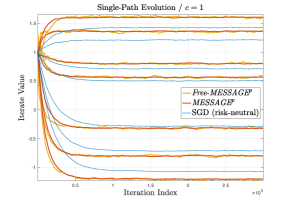
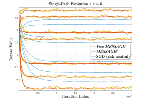
Figure 7.1: Single-path evolution of $\textit{Free-MESSAGE}^{p}$, $\textit{MESSAGE}^{p}$ and Stochastic Gradient Descent (SGD) for the problem setting considered in Section 7, and for two values of $c$ (left, right).

Fig. 7.1 shows the evolution of all seven entries of the regressor process $\{\boldsymbol{x}^{n}\}_{n\in\mathbb{N}_{T}}$, for both algorithms considered and for two values of $c$, namely, $c\equiv 1$ (left) and $c\equiv 5$ (right). Recall that if $c\in[0,1]$, then the risk-aware ridge regression problem at hand is strongly convex. Also, although convexity is not guaranteed if $c>1$, in such a case the problem is expected to be at least weakly convex (at least approximately); this is due to the smoothness of $F_{\sigma}$ and the Gaussian smoothing involved in the construction of the surrogate $\phi_{\mu}$ (in the case of $\textit{Free-MESSAGE}^{p}$, pertaining to our analysis). In the figure, we also provide comparatively the paths generated by standard Stochastic Gradient Descent (SGD) with constant stepsize $\alpha$, to highlight the substantial difference in the solutions of the learning problem between the risk-neutral (i.e., $c\equiv 0$) and risk-aware settings, respectively.

For both values of $c$, Fig. 7.1 clearly demonstrates that $\textit{Free-MESSAGE}^{p}$ closely mimics $\textit{MESSAGE}^{p}$, and that both algorithms converge to a stable neighborhood of the optimal regressor (hopefully for $c\equiv 5$) at an identical linear rate. In particular, for $c\equiv 1$ (where strong convexity is ensured), this behavior is in agreement with our theoretical results. We further observe that the price paid for the lack of first-order information is noisier and more sensitive zeroth-order quasigradients, as indicated by the larger fluctuations of the iterates generated by $\textit{Free-MESSAGE}^{p}$. Those fluctuations increase when $c\equiv 5$; this is expected, because the magnitude of the quasigradients of $\textit{Free-MESSAGE}^{p}$ is proportional to $c$. Still, we clearly observe that $\textit{Free-MESSAGE}^{p}$ exhibits very consistent behavior as compared with its gradient-based counterpart.

At this point, we would also like to note that in worse-conditioned problems than our indicative example where two-sample-based zeroth-order quasigradients might be too noisy, one can reformulate $\textit{Free-MESSAGE}^{p}$ in an almost straightforward way by incorporating Gaussian minibatching for quasigradient stabilization (see, e.g., [16], Section 5), and with little additional effort in the corresponding convergence analysis. However, minibatching comes at the expense of additional sampling requirements.

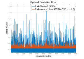
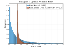
Figure 7.2: Prediction (test) errors achieved by $\textit{Free-MESSAGE}^{p}$ and SGD, for the problem setting considered in Section 7 with $c\equiv 2.5$ (left: error values, right: corresponding histogram).

Additionally, $\textit{Free-MESSAGE}^{p}$ is favorably comparable to $\textit{MESSAGE}^{p}$ in terms of computational requirements. While the throughput of the two algorithms is exactly the same ($1:2$, since each iteration requires two learning examples), the complexity per iteration of $\textit{Free-MESSAGE}^{p}$ is expected to be smaller, since $\textit{Free-MESSAGE}^{p}$ relies only on four function evaluations and elementary vector (not matrix) operations. This holds under the reasonable assumption that that full gradient evaluations are generally more complex than evaluations of cost function values. The only additional computational requirement of $\textit{Free-MESSAGE}^{p}$ over $\textit{MESSAGE}^{p}$ is that of a Gaussian sampler, which is really rather trivial for most practical considerations.

Lastly, the effects of the solutions achieved by $\textit{Free-MESSAGE}^{p}$ (or $\textit{MESSAGE}^{p}$) and SGD on the resulting optimal prediction errors are shown in Fig. 7.2 (for $c\equiv 2.5$). The premise of risk-aware statistical learning is to effectively control the statistical dispersion of the random cost associated with a particular learning task. In statistical regression, this translates to a desire to ensure optimal prediction error stability, also reasonably trading with keeping as small mean prediction error as possible; this is exactly what Fig. 7.2 illustrates for our risk-aware regression example. We observe that the reduction in the volatility of the instantaneous prediction errors achieved by the risk-aware solution is rather drastic as compared with the risk-neutral solution (left), also translating to a much tighter corresponding empirical distribution (right). Of course, the price to be paid for an optimal risk-aware regressor is a higher average regression cost; this is natural and expected, since the ultimately minimum average cost is achieved by the risk-neutral solution, which is recovered by setting $c\equiv 0$.

Remark 7.1.

The fact that convergence of $\textit{(Free-)MESSAGE}^{p}$ appears to be faster than that of stochastic gradient descent in Fig. 7.1 does not of course imply that risk-aware ridge regression is in general simpler and/or easier than risk-neutral ridge regression, as the two problems are structurally very different. In fact, the opposite is most probably true, especially for higher-dimensional problems. Also, the convergence rate achieved by stochastic gradient descent for our ridge regression example can be significantly and stably accelerated by using a more aggressive stepsize.

8 Future Work

There are several interesting topics for future work, building on the results presented in this paper; indicatively, we discuss some. First, although our rate results quantify explicitly the dependence on $\mu$ and $\sigma$, we have not paid much attention to the decision dimension, $N$. Indeed, if $c\equiv 0$, then, orderwise relative to $N$, our bounds are equivalent to those in [30], known to be order-suboptimal (see, e.g., [12]). Therefore, it would be of interest to see if order improvement relative to $N$ is possible, by potentially exploiting ideas from more ingenious methods for risk-neutral zeroth-order optimization, such as those with diminishing $\mu$, multi-point finite differences, and/or minibatching. Second, also driven by [12], another challenging topic is the development of lower complexity bounds for risk-aware learning, which would be useful in the design of optimal algorithms and, of course, as complexity benchmarks. Lastly, further relaxing the convexity of the base problem is of particular interest, as the resulting setting fits more accurately many application settings in modern artificial intelligence and deep learning.

Appendix A Proof of Lemma 3.4

If $\mu\equiv 0$, the situation is trivial. So, for the rest of the proof, we assume that $\mu>0$. Let ${\cal N}:\mathbb{R}^{N}\rightarrow\mathbb{R}$ be the standard Gaussian density on $\mathbb{R}^{N}$. We first make the observation that, for every finite $B>0$,

$${\cal N}\left(\dfrac{\boldsymbol{u}}{\mu}\right)\exp\left(\dfrac{\left\|\boldsymbol{u}\right\|_{2}B}{\mu^{2}}\right)\max\{1,\left\|\boldsymbol{u}\right\|_{2}\} \propto\exp\left(-\dfrac{\left\|\boldsymbol{u}\right\|_{2}^{2}}{2\mu^{2}}\right)\exp\left(\dfrac{\left\|\boldsymbol{u}\right\|_{2}B}{\mu^{2}}\right)\max\{1,\left\|\boldsymbol{u}\right\|_{2}\}$$

$$\leq\exp\left(-\dfrac{\left\|\boldsymbol{u}\right\|_{2}^{2}}{2\mu^{2}}+\dfrac{\left\|\boldsymbol{u}\right\|_{2}B}{\mu^{2}}+\left\|\boldsymbol{u}\right\|_{2}\right)$$

$$\leq\exp\left(-\dfrac{\left\|\boldsymbol{u}\right\|_{2}^{2}}{2\mu_{\star}^{2}}\right),$$

provided that $\mu<\mu_{\star}$ and $\left\|\boldsymbol{u}\right\|_{2}\geq\big{(}2(B+\mu^{2})\mu_{\star}^{2}\big{)}/\big{(}\mu_{\star}^{2}-\mu^{2}\big{)}$. Consequently, as long as condition (3) is in effect, it readily follows that

$$\int{\cal N}\left(\dfrac{\boldsymbol{u}}{\mu}\right)\exp\left(\dfrac{\left\|\boldsymbol{u}\right\|_{2}B}{\mu^{2}}\right)\max\{1,\left\|\boldsymbol{u}\right\|_{2}\}|f(\boldsymbol{u})|\mathrm{d}\boldsymbol{u}<\infty.$$

To see why this is important, recall the definition of $f_{\mu}(\cdot)\equiv\mathbb{E}\{f((\cdot)+\mu\boldsymbol{U})\}$, for which is must be true that

$$\mathbb{E}\{|f(\boldsymbol{x}+\mu\boldsymbol{U})|\} \equiv\mu^{-N}\int|f\left(\boldsymbol{u}\right)|\hskip 1.0pt{\cal N}\left(\dfrac{\boldsymbol{x}-\boldsymbol{u}}{\mu}\right)\mathrm{d}\boldsymbol{u}$$

$$\leq\mu^{-N}\int|f\left(\boldsymbol{u}\right)|\hskip 1.0pt{\cal N}\left(\dfrac{\boldsymbol{u}}{\mu}\right)\exp\left(\dfrac{\left\|\boldsymbol{u}\right\|_{2}\left\|\boldsymbol{x}\right\|_{2}}{\mu^{2}}\right)\mathrm{d}\boldsymbol{u}<\infty,$$

from where it follows that the random function $f\left(\boldsymbol{x}+\mu\boldsymbol{U}\right)$ in ${\cal Z}_{1}$, for all $\boldsymbol{x}\in\mathbb{R}^{N}$. Equivalently, we have shown that the function $f_{\mu}\left(\cdot\right)\equiv\mathbb{E}\left\{f\left(\left(\cdot\right)+\mu\boldsymbol{U}\right)\right\}$ is well-defined and finite, everywhere on $\mathbb{R}^{N}$. The rest of the first part, and the second part of Lemma 3.4 may be developed along the lines of [30], where we explicitly use the identity $\mathbb{E}\left\{\mathsf{T}\left(\boldsymbol{x},\boldsymbol{U}\right)\right\}\equiv 0$, for all $\boldsymbol{x}\in{\cal F}$, since $\mathsf{T}$ is a normal remainder on ${\cal F}$.

For the third part, the result on the existence and representation of $\nabla f_{\mu}$ will follow by a careful application of the Dominated Convergence Theorem, which provides an extension of the standard Leibniz rule of Riemann integration, and permits interchangeability of differentiation and integration. Specifically, we will exploit a multidimensional version of ([13], Theorem 2.27). To this end, for $\mu>0$, define

$$\varphi\left(\boldsymbol{x},\boldsymbol{u}\right)\triangleq f\left(\boldsymbol{u}\right)\mu^{-N}{\cal N}\left(\dfrac{\boldsymbol{x}-\boldsymbol{u}}{\mu}\right),\quad\left(\boldsymbol{x},\boldsymbol{u}\right)\in{\cal F}\times\mathbb{R}^{N}.$$

By our construction, $\varphi\left(\boldsymbol{x},\cdot\right)$ is Lebesgue integrable on $\mathbb{R}^{N}$ for every $\boldsymbol{x}\in\mathbb{R}^{N}$, and $\varphi\left(\cdot,\boldsymbol{u}\right)$ is differentiable everywhere on $\mathbb{R}^{N}$ for every $\boldsymbol{u}\in\mathbb{R}^{N}$, with

$$\nabla_{\boldsymbol{x}}\varphi\left(\boldsymbol{x},\boldsymbol{u}\right)\equiv\mu^{-N-2}f\left(\boldsymbol{u}\right){\cal N}\left(\dfrac{\boldsymbol{u}-\boldsymbol{x}}{\mu}\right)\left(\boldsymbol{u}-\boldsymbol{x}\right).$$

Now, consider any compact box ${\cal B}\subseteq\mathbb{R}^{N}$. Choosing $B\triangleq\sup_{\boldsymbol{x}\in{\cal B}}\left\|\boldsymbol{x}\right\|_{2}$ and for every $\boldsymbol{u}\in\mathbb{R}^{N}$, we may write

$$\left\|\nabla_{\boldsymbol{x}}\varphi\left(\boldsymbol{x},\boldsymbol{u}\right)\right\|_{2} \leq\mu^{-N-2}\hskip 1.0pt{\cal N}\left(\dfrac{\boldsymbol{u}-\boldsymbol{x}}{\mu}\right)\left|f\left(\boldsymbol{u}\right)\right|\left(\left\|\boldsymbol{u}\right\|_{2}+\left\|\boldsymbol{x}\right\|_{2}\right)$$

$$\leq\mu^{-N-2}\left(1+B\right){\cal N}\left(\dfrac{\boldsymbol{u}}{\mu}\right)\exp\left(\dfrac{\left\|\boldsymbol{u}\right\|_{2}B}{\mu^{2}}\right)\max\{1,\left\|\boldsymbol{u}\right\|_{2}\}\left|f\left(\boldsymbol{u}\right)\right|\triangleq\psi_{{\cal B}}\left(\boldsymbol{u}\right).$$

Note that the use of the $\ell_{2}$-norm is arbitrary; any (equivalent) vector norm works. The analysis in the beginning of the proof implies that $\psi_{{\cal B}}$ has a finite Lebesgue integral on $\mathbb{R}^{N}$. Therefore, it is true that $\sup_{\boldsymbol{x}\in{\cal B}}\left\|\nabla_{\boldsymbol{x}}\varphi\left(\boldsymbol{x},\cdot\right)\right\|_{2}\leq\psi_{{\cal B}}\left(\cdot\right)\in{\cal L}_{1}\big{(}\mathbb{R}^{N},\mathscr{\mathscr{B}}\bigl{(}\mathbb{R}^{N}\bigr{)},\lambda;\mathbb{R}\big{)}$, where $\lambda:\text{$\mathscr{\mathscr{B}}\bigl{(}\mathbb{R}^{M}\bigr{)}$}\rightarrow\mathbb{R}_{+}$ denotes the corresponding Lebesgue measure. It then follows that the function $f_{\mu}\left(\cdot\right)\equiv\int\varphi\left(\cdot,\boldsymbol{u}\right)\text{d}\boldsymbol{u}$ is differentiable on ${\cal B}$, and that

$$\nabla f_{\mu}\left(\boldsymbol{x}\right) \equiv\int\nabla_{\boldsymbol{x}}\varphi\left(\boldsymbol{x},\boldsymbol{u}\right)\text{d}\boldsymbol{u}$$

$$=\int\mu^{-1}f\left(\boldsymbol{x}+\mu\boldsymbol{u}\right){\cal N}\left(\boldsymbol{u}\right)\boldsymbol{u}\text{d}\boldsymbol{u}-\int\mu^{-1}f\left(\boldsymbol{x}\right){\cal N}\left(\boldsymbol{u}\right)\boldsymbol{u}\text{d}\boldsymbol{u}$$

$$\equiv\int\dfrac{f\left(\boldsymbol{x}+\mu\boldsymbol{u}\right)-f\left(\boldsymbol{x}\right)}{\mu}\boldsymbol{u}\hskip 1.0pt{\cal N}\left(\boldsymbol{u}\right)\text{d}\boldsymbol{u},$$

for every $\boldsymbol{x}\in{\cal B}$ (Theorem 2.27 in [13]). But the box ${\cal B}$ is arbitrary, and any $\boldsymbol{x}\in\mathbb{R}^{N}$ is contained in a compact box. For the rest of the third part of Lemma 3.4, if $f$ is $\left(L,\mathsf{D},\mathsf{T}\right)$-SLipschitz on ${\cal F}$, we may write

$$\mathbb{E}\left\{\bigg{\|}\dfrac{f\left(\boldsymbol{x}+\mu\boldsymbol{U}\right)-f\left(\boldsymbol{x}\right)}{\mu}\boldsymbol{U}\bigg{\|}_{2}^{2}\right\}$$

$$\equiv\dfrac{1}{\mu^{2}}\mathbb{E}\big{\{}|f\left(\boldsymbol{x}+\mu\boldsymbol{U}\right)-f\left(\boldsymbol{x}\right)-\mathsf{T}\left(\boldsymbol{x},\mu\boldsymbol{U}\right)+\mathsf{T}\left(\boldsymbol{x},\mu\boldsymbol{U}\right)|^{2}\left\|\boldsymbol{U}\right\|_{2}^{2}\big{\}}$$

$$\leq\dfrac{1}{\mu^{2}}\mathbb{E}\big{\{}\big{(}L\mathsf{D}\left(\mu\boldsymbol{U}\right)+|\mathsf{T}\left(\boldsymbol{x},\mu\boldsymbol{U}\right)|\big{)}^{2}\left\|\boldsymbol{U}\right\|_{2}^{2}\big{\}},$$

for all $\boldsymbol{x}\in{\cal F}$. Enough said.

References

• [1] P. L. A. and M. Fu, Risk-sensitive reinforcement learning: A constrained optimization viewpoint, arXiv preprint, arXiv:1810.09126, (2018), https://arxiv.org/abs/1810.09126.
• [2] S. Ahmed, U. Çakmak, and A. Shapiro, Coherent risk measures in inventory problems, European Journal of Operational Research, 182 (2007), pp. 226–238, https://doi.org/10.1016/j.ejor.2006.07.016.
• [3] R. B. Ash and C. Doléans-Dade, Probability and Measure Theory, Academic Press, 2000, https://doi.org/10.2307/2291440, https://arxiv.org/abs/arXiv:1011.1669v3.
• [4] K. Balasubramanian and S. Ghadimi, Zeroth-rder (non)-convex stochastic optimization via conditional gradient and gradient updates, in Advances in Neural Information Processing Systems, vol. 2018-Decem, 2018, pp. 3455–3464.
• [5] A. S. Bedi, A. Koppel, and K. Rajawat, Nonparametric compositional stochastic optimization, arXiv preprint, arXiv:1902.06011, (2019), https://arxiv.org/abs/1902.06011.
• [6] S. Bruno, S. Ahmed, A. Shapiro, and A. Street, Risk neutral and risk-averse approaches to multistage renewable investment planning under uncertainty, European Journal of Operational Research, 250 (2016), pp. 979–989, https://doi.org/10.1016/j.ejor.2015.10.013.
• [7] A. R. Cardoso and H. Xu, Risk-averse stochastic convex bandit, in International Conference on Artificial Intelligence and Statistics, vol. 89, Apr. 2019, pp. 39–47.
• [8] Y. Chen, H. Chang, J. Meng, and D. Zhang, Ensemble neural networks (enn): A gradient-free stochastic method, Neural Networks, 110 (2019), pp. 170–185, https://doi.org/10.1016/j.neunet.2018.11.009.
• [9] Z. Chen and Y. Wang, Two-sided coherent risk measures and their application in realistic portfolio optimization, Journal of Banking and Finance, 32 (2008), pp. 2667–2673, https://doi.org/10.1016/j.jbankfin.2008.07.004.
• [10] A. R. A. R. Conn, K. Scheinberg, and L. N. Vicente, Introduction to Derivative-Free Optimization, Society for Industrial and Applied Mathematics/Mathematical Programming Society, 2009.
• [11] D. Davis and D. Drusvyatskiy, Stochastic model-based minimization of weakly convex functions, SIAM Journal on Optimization, 29 (2019), pp. 207–239, https://doi.org/10.1137/18M1178244, https://arxiv.org/abs/1803.06523.
• [12] J. C. Duchi, M. I. Jordan, M. J. Wainwright, and A. Wibisono, Optimal rates for zero-order convex optimization: The power of two function evaluations, IEEE Transactions on Information Theory, 61 (2015), pp. 2788–2806, https://doi.org/10.1109/TIT.2015.2409256.
• [13] G. B. Folland, Real Analysis: Modern Techniques and their Applications, John Wiley & Sons, 2nd ed., 1999.
• [14] T. Fu, X. Zhuang, Y. Hui, and J. Liu, Convex risk measures based on generalized lower deviation and their applications, International Review of Financial Analysis, 52 (2017), pp. 27–37, https://doi.org/10.1016/j.irfa.2017.04.008.
• [15] S. Ghadimi and G. Lan, Stochastic first- and zeroth-order methods for nonconvex stochastic programming, SIAM Journal on Optimization, 23 (2013), pp. 2341–2368, https://doi.org/10.1137/120880811, https://arxiv.org/abs/1309.5549.
• [16] S. Ghadimi, G. Lan, and H. Zhang, Mini-batch stochastic approximation methods for nonconvex stochastic composite optimization, Mathematical Programming, 155 (2016), pp. 267–305, https://doi.org/10.1007/s10107-014-0846-1.
• [17] I. Goodfellow, Y. Bengio, and A. Courville, Deep learning, MIT Press, 2016.
• [18] J.-y. Gotoh and S. Uryasev, Support vector machines based on convex risk functions and general norms, Annals of Operations Research, 249 (2017), pp. 301–328, https://doi.org/10.1007/s10479-016-2326-x.
• [19] D. Hajinezhad and M. M. Zavlanos, Gradient-free multi-agent nonconvex nonsmooth optimization, in Proceedings of the IEEE Conference on Decision and Control, vol. 2018-Decem, IEEE, Dec. 2019, pp. 4939–4944, https://doi.org/10.1109/CDC.2018.8619333.
• [20] T. Hastie, R. Tibshirani, and J. Friedman, The Elements of Statistical Learning, Springer Series in Statistics, Springer New York, New York, NY, 2009, https://doi.org/10.1007/978-0-387-84858-7.
• [21] W. Huang and W. B. Haskell, Risk-aware q-learning for markov decision processes, in 2017 IEEE 56th Annual Conference on Decision and Control, CDC 2017, vol. 2018-Janua, IEEE, Dec. 2018, pp. 4928–4933, https://doi.org/10.1109/CDC.2017.8264388.
• [22] D. R. Jiang and W. B. Powell, Risk-averse approximate dynamic programming with quantile-based risk measures, Mathematics of Operations Research, 43 (2018), pp. 554–579, https://doi.org/10.1287/moor.2017.0872, https://arxiv.org/abs/1509.01920.
• [23] D. S. Kalogerias and W. B. Powell, Recursive optimization of convex risk measures: Mean-semideviation models, arXiv preprint, arXiv:1804.00636, (2018), https://arxiv.org/abs/1804.00636.
• [24] S.-K. Kim, R. Thakker, and A.-a. Agha-mohammadi, Bi-directional value learning for risk-aware planning under uncertainty, IEEE Robotics and Automation Letters, 4 (2019), pp. 2493–2500, https://doi.org/10.1109/LRA.2019.2903259, https://arxiv.org/abs/1902.05698.
• [25] W.-J. Ma, C. Oh, Y. Liu, D. Dentcheva, and M. M. Zavlanos, Risk-averse access point selection in wireless communication networks, IEEE Transactions on Control of Network Systems, 5870 (2018), pp. 1–1, https://doi.org/10.1109/TCNS.2018.2792309.
• [26] S. Moazeni, W. B. Powell, B. Defourny, and B. Bouzaiene-Ayari, Parallel nonstationary direct policy search for risk-averse stochastic optimization, INFORMS Journal on Computing, 29 (2017), pp. 332–349, https://doi.org/10.1287/ijoc.2016.0733.
• [27] S. Moazeni, W. B. Powell, and A. H. Hajimiragha, Mean-conditional value-at-risk optimal energy storage operation in the presence of transaction costs, IEEE Transactions on Power Systems, 30 (2015), pp. 1222–1232, https://doi.org/10.1109/TPWRS.2014.2341642.
• [28] J. Moreau, Proximité et dualité dans un espace hilbertien, Bulletin de la Société mathématique de France, 79 (1965), pp. 273–299, https://doi.org/10.24033/bsmf.1625.
• [29] A. S. Nemirovsky and D. B. Yudin, Problem Complexity and Method Efficiency in Optimization, John Wiley & Sons, New York, 1983.
• [30] Y. Nesterov and V. Spokoiny, Random gradient-free minimization of convex functions, Foundations of Computational Mathematics, 17 (2017), pp. 527–566, https://doi.org/10.1007/s10208-015-9296-2.
• [31] M. Norton, A. Mafusalov, and S. Uryasev, Soft margin support vector classification as buffered probability minimization, Journal of Machine Learning Research, 18 (2017), pp. 1–43.
• [32] W. Ogryczak and A. Ruszczyński, From stochastic dominance to mean-risk models: Semideviations as risk measures, European Journal of Operational Research, 116 (1999), pp. 33–50, https://doi.org/10.1016/S0377-2217(98)00167-2.
• [33] W. Ogryczak and A. Ruszczyński, Dual stochastic dominance and related mean-risk models, SIAM Journal on Optimization, 13 (2002), pp. 60–78, https://doi.org/10.1137/S1052623400375075.
• [34] A. A. Pereira, J. Binney, G. A. Hollinger, and G. S. Sukhatme, Risk-aware path planning for autonomous underwater vehicles using predictive ocean models, Journal of Field Robotics, 30 (2013), pp. 741–762, https://doi.org/10.1002/rob.21472.
• [35] R. T. Rockafellar, S. Uryasev, and M. Zabarankin, Generalized deviations in risk analysis, Finance and Stochastics, 10 (2006), pp. 51–74, https://doi.org/10.1007/s00780-005-0165-8.
• [36] T. R. Rockafellar, S. P. Uryasev, and M. Zabarankin, Deviation measures in risk analysis and optimization, SSRN Electronic Journal, (2003), https://doi.org/10.2139/ssrn.365640.
• [37] A. Sani, A. Lazaric, and R. Munos, Risk-aversion in multi-armed bandits, in Advances in Neural Information Processing Systems 25 (NIPS 2012), 2012, pp. 3275–3283.
• [38] D. Shang, V. Kuzmenko, and S. Uryasev, Cash flow matching with risks controlled by buffered probability of exceedance and conditional value-at-risk, Annals of Operations Research, 260 (2018), pp. 501–514, https://doi.org/10.1007/s10479-016-2354-6.
• [39] A. Shapiro, D. Dentcheva, and A. Ruszczyński, Lectures on Stochastic Programming: Modeling and Theory, Society for Industrial and Applied Mathematics, 2nd ed., 2014, https://doi.org/http://dx.doi.org/10.1137/1.9780898718751.
• [40] J. C. Spall, Introduction to Stochastic Search and Optimization: Estimation, Simulation, and Control, Wiley-Interscience, 2003.
• [41] A. Tamar, Y. Chow, M. Ghavamzadeh, and S. Mannor, Sequential decision making with coherent risk, IEEE Transactions on Automatic Control, 62 (2017), pp. 3323–3338, https://doi.org/10.1109/TAC.2016.2644871.
• [42] G. Taylor, R. Burmeister, Z. Xu, B. Singh, A. Patel, and T. Goldstein, Training neural networks without gradients: A scalable admm approach, in 33rd International Conference on Machine Learning (ICML 2016), June 2016, pp. 2722–2731, https://arxiv.org/abs/1605.02026.
• [43] V. N. Vapnik, The Nature of Statistical Learning Theory, Springer, 2000.
• [44] C. A. Vitt, D. Dentcheva, and H. Xiong, Risk-averse classification, Annals of Operations Research, (2019), https://doi.org/10.1007/s10479-019-03344-6, https://arxiv.org/abs/1805.00119.
• [45] M. Wang, E. X. Fang, and H. Liu, Stochastic compositional gradient descent: Algorithms for minimizing compositions of expected-value functions, Mathematical Programming, 161 (2017), pp. 419–449, https://doi.org/10.1007/s10107-016-1017-3, https://arxiv.org/abs/1411.3803.
• [46] S. Yang, M. Wang, and E. X. Fang, Multilevel stochastic gradient methods for nested composition optimization, SIAM Journal on Optimization, 29 (2019), pp. 616–659, https://doi.org/10.1137/18M1164846.
• [47] P. Yu, W. B. Haskell, and H. Xu, Approximate value iteration for risk-aware markov decision processes, IEEE Transactions on Automatic Control, 63 (2018), pp. 3135–3142, https://doi.org/10.1109/TAC.2018.2790261, https://arxiv.org/abs/1701.01290.
• [48] D. Yuan and D. W. Ho, Randomized gradient-free method for multiagent optimization over time-varying networks, IEEE Transactions on Neural Networks and Learning Systems, 26 (2015), pp. 1342–1347, https://doi.org/10.1109/TNNLS.2014.2336806.
• [49] L. Zhou and P. Tokekar, An approximation algorithm for risk-averse submodular optimization, arXiv preprint, arXiv:1807.09358, (2018), https://doi.org/10.1007/978-3-030-44051-0_9, https://arxiv.org/abs/1807.09358.