Abstract

We address the problem of minimizing a smooth function $f^{0}(x)$ over a compact set $D$ defined by smooth functional constraints $f^{i}(x)\leq 0,\leavevmode\nobreak\ i=1,\ldots,m$ given noisy value measurements of $f^{i}(x)$. This problem arises in safety-critical applications, where certain parameters need to be adapted online in a data-driven fashion, such as in personalized medicine, robotics, manufacturing, etc. In such cases, it is important to ensure constraints are not violated while taking measurements and seeking the minimum of the cost function. We propose a new algorithm s0-LBM, which provides provably feasible iterates with high probability and applies to the challenging case of uncertain zero-th order oracle. We also analyze the convergence rate of the algorithm, and empirically demonstrate its effectiveness.

1 INTRODUCTION

Many applications in robotics (Schaal and Atkeson,, 2010), manufacturing (Maier et al.,, 2018), health sciences, finance, etc. require minimizing a loss function under constraints and uncertainty. Optimizing a loss function under partially revealed constraints can be further complicated by the fact that observations are available only inside the feasible set. Hence, one needs to carefully choose actions to ensure the feasibility of each iterate while pursuing the optimal solution. In the machine learning community, this problem is known as safe learning. For such tasks, feasible optimization methods are required. There are many first and second order feasible methods in the literature. Although given noisy zero-th order oracle the Hessians are hard to estimate with good accuracy, we can approximate derivatives using finite differences. Most well known and widely used first order methods for stochastic optimization are dealing with constraints using projections. However, the lack of global knowledge of the constraint functionals makes it impossible to compute the corresponding projection operator.

Related work.

There is a lack of zero-th order feasible (safe) algorithms for black-box constrained optimization in the literature. Balasubramanian and Ghadimi, (2018) provide a comprehensive analysis of the performance of several zero-th order algorithms for non-convex optimization. However, the conditional gradient based algorithm (Frank-Wolfe) of Balasubramanian and Ghadimi, (2018) for constrained non-convex problems requires global knowledge of the constraint functions, as the linear objective must be optimized with respect to these constraints. Usmanova et al., (2019) introduce a Frank-Wolfe based algorithm applied to the case of noisy zero-th order oracle for linear constraints. This work proves the feasibility of iterates with high probability and bounded the convergence rate with high probability, but does require convexity.

Non-convex non-smooth problems can be addressed by feasible methods, such as the first order Method of Feasible Directions (Topkis and Veinott,, 1967) or the second order Feasible Sequential Quadratic Programming (FSQP) algorithm (Tang et al.,, 2014). Another algorithm for non-convex non-smooth problems is given by Facchinei et al., (2017). The idea of this algorithm is to use as a direction of movement the minimizer of a local convex approximation of the objective subject to a local convex approximation of constraint set. Unfortunately, all the guarantees for the above methods are in terms of asymptotic convergence to a stationary point.

Another class of safe algorithms for global black-box optimization is based on Bayesian Optimization(BO) such as SafeOpt (Sui et al.,, 2015) and its extensions (Berkenkamp et al.,, 2016). The main drawback of these methods is that the computational complexity grows exponentially with dimensionality.

Interior Point Methods (IPM) are feasible approaches by definition, and they are widely used for Linear Programming, Quadratic Programming, and Conic optimization problems. By using self-concordance properties of specifically chosen barriers and second order information, these problems are shown to be extremely efficiently solved by IPM. However, in the cases when constraints are unknown, building the barrier with self-concordance properties is not possible. In these cases it is possible to use logarithmic barriers for general black-box constraints. Hinder and Ye, (2018) propose to choose adaptive step sizes for the gradient algorithm for the log barriers and give the analysis of the convergence rate. The work of Hinder and Ye, (2018) assume knowledge of the exact gradients of the cost and constraint functions. In the present work, we extend this approach for the case in which we only have a possibly noisy zero-th order oracle.

Our Contributions.

In this paper we propose the first safe zero-th order algorithm for non-convex optimization with a black-box noisy oracle. We prove that it generates feasible iterations with high probability, and analyse its convergence rate to the local optimum. Each iteration is computationally very cheap and does not require solving any subproblems such as those required for Frank-Wolfe or Bayesian Optimization based algorithms. In Table 1, we provide a comparison of our algorithm with the existing ones for unconstrained and constrained zero-th order non-convex optimization. In the first two algorithms a multiple point feedback is assumed, i.e., it is possible to measure at several points with the same noise realization. The convergence rate in the second column is proven for known polyhedral constraints. In our algorithm we assume a more realistic and more complicated setup where the noise is changing with each measurement. There are some works in zero-th order 1-point feedback for convex optimization with known constraints, for example Bach and Perchet, (2016) require $O\left(\frac{d^{2}}{\eta^{3}}\right)$ measurements to achieve $\eta$ accuracy.

Problem	Unconstrained	Known constraints	Safe despite unknown constraints
Feedback	Noisy 2-point	Noisy 2-point	Noisy 1-point
Optimality criterion	Stationary point: $\mathbb{E}\|\nabla f(x_{t})\|_{2}\leq\eta$	$\eta$-stationary point: $\mathbb{E}\langle\nabla f(x_{t}),x_{t}-u\rangle\leq\eta\forall u\in D$	$\eta$-approximate scaled KKT point: $\mathbb{P}\{\|\nabla L(x_{t})\|_{2}\leq\eta(1+\|\lambda_{t}\|_{\infty})\}\geq 1-\delta$
Number of measurements	$O\left(\frac{d}{\eta^{4}}\right)$ (no matrix inversion) $O\left(\frac{d}{\eta^{3.5}}\right)+\tilde{O}\left(\frac{d^{4}}{\eta^{2.5}}\right)$ (hessian estimation) (Balasubramanian, Ghadimi, 2018)	$O\left(\frac{d}{\eta^{4}}\right)$ (conditional gradient based, requires $O\left(\frac{1}{\eta^{2}}\right)$ optimization subproblems w.r.t. $D$) (Balasubramanian, Ghadimi, 2018)	$\tilde{O}\left(\frac{d^{3}}{\eta^{7}}\sqrt{\ln 1/\delta}\right)$ ($O\left(\frac{1}{\eta^{3}}\right)steps$) (this paper, does not require solving subproblems or matrix inversions)

Table 1: Upper $O(\cdot)$ bounds on number of zero-th order oracle calls for non-convex smooth optimization.

2 PROBLEM STATEMENT

Notations and definitions.

Let $\|\cdot\|_{2}$,$\|\cdot\|_{1}$ and $\|\cdot\|_{\infty}$ denote $l_{2}$-norm, $l_{1}$-norm and $l_{\infty}$-norm respectively on $\mathbb{R}^{d}$. A function $f(x)$ is called $L$-Lipschitz continuous if

$$|f(x)-f(y)|\leq L\|x-y\|_{2}.$$ (1)

It is called $M$-smooth if the gradients $\nabla f(x)$ are $M$-Lipschitz continuous, i.e.,

$$\|\nabla f(x)-\nabla f(y)\|_{2}\leq M\|x-y\|_{2}.$$ (2)

A random variable $\xi$ is zero-mean $\sigma$-sub-Gaussian if

$$\forall\lambda\in\mathbb{R}\leavevmode\nobreak\ \mathbb{E}\left[e^{\lambda\xi}\right]\leq\text{exp}\left(\frac{\lambda^{2}\sigma^{2}}{2}\right),$$

which implies that $\text{Var}\left[\xi\right]\leq\sigma^{2}$.

Problem formulation

We consider the problem of non-convex safe learning defined as a constrained optimization problem

$$\min_{x\in\mathbb{R}^{d}}\leavevmode\nobreak\ \leavevmode\nobreak\ \leavevmode\nobreak\ \leavevmode\nobreak\ \leavevmode\nobreak\ \leavevmode\nobreak\ \leavevmode\nobreak\ f^{0}(x)$$

$$\text{subject to }f^{i}(x)\leq 0,\leavevmode\nobreak\ \leavevmode\nobreak\ i=1,\ldots,m,$$ (3)

where the objective function $f^{0}:\mathbb{R}^{d}\rightarrow\mathbb{R}$ and the constraints $f^{i}:\mathbb{R}^{d}\rightarrow\mathbb{R}$ are unknown continuous functions, and can only be accessed at feasible points $x$. We denote by $D$ the feasible set $D:=\{x\in\mathbb{R}^{d}:f^{i}(x)\leq 0,i=1,\ldots,m\}.$

Assumption 1.

Let $M,L>0$. The objective and the constraint functions $f^{i}(x)$ for $i=0,\ldots,m$ are $M$-smooth on $D$. Also, constraint functions $f^{i}(x)$ for $i=1,\ldots,m$ are $L$-Lipschitz continuous on $D$.

Assumption 2.

The feasible set $D$ has a non-empty interior, and there exists a known starting point $x_{0}$ for which $f^{i}(x_{0})<0$ for $i=1,\ldots,m.$

Oracle information.

We consider zero-th order oracle information. If we can measure the function values exactly, then one possible oracle is the Exact Zero-th Order oracle (EZO).
EZO: provides the exact values $f^{i}(x_{t})\leavevmode\nobreak\ \forall i=0,\ldots,m$ for any requested point $x_{t}\in D.$

In many applications, the measurements of the functions are noisy. We assume that the additive noise $\xi$ is coming from a zero-mean $\sigma$-sub-Gaussian distribution. We call this oracle Stochastic Zero-th Order oracle (SZO).
SZO: $\forall i=0,\ldots,m$ provides the noisy function values $F^{i}(x_{t},\xi^{i}_{t})=f^{i}(x_{t})+\xi^{i}_{t}$, $\xi^{i}_{t}$ is a zero-mean $\sigma$-sub-Gaussian noise independent of previous measurements for any requested point $x_{t}\in D$. We assume that the noise values $\xi^{i}_{t}$ are independent over time $t$ and indices $i$.

Optimality criterion.

The condition $\|\nabla f^{0}(x_{T})\|_{2}\leq\varepsilon$ is usually used as an optimality criterion in non-convex smooth optimization without constraints. It is well known that in the unconstrained case the classical gradient descent method converges with rate $O(\frac{1}{\varepsilon^{2}}),$ which matches the lower bound derived for this class of problems (Carmon et al.,, 2017). In the non-convex constrained optimization, first order criteria are Karush-Kuhn-Tucker (KKT) conditions, which are necessary in the presence of regularity conditions called Constraint Qualification (CQ). In such cases, we can measure the solution accuracy by satisfying approximate KKT conditions. The point $(x,\lambda)\in\mathbb{R}^{n}\times\mathbb{R}^{m}$ is called a KKT point if it satisfies the necessary condition for local optimality:

$$\lambda^{i},-f^{i}(x)\geq 0,\leavevmode\nobreak\ \forall i=1,\ldots,m$$

$$\lambda^{i}(-f^{i}(x))=0,\leavevmode\nobreak\ \forall i=1,\ldots,m$$

$$\|\nabla L(x,\lambda)\|_{2}=0,$$

where $\lambda$ is the vector of dual variables and $L(x,\lambda):=f^{0}(x)+\sum_{i=1}^{m}\lambda^{i}f^{i}(x)$ is the Lagrangian. There are several ways to define an approximate KKT point, see (Cartis et al.,, 2014; Birgin et al.,, 2016). Similar to Cartis et al., (2014), we define an approximate KKT point as follows. An $\eta$-approximate scaled KKT point (s-KKT) for some $\eta>0$ is a pair $(x,\lambda)$ which satisfies:

$$\lambda^{i},-f^{i}(x)\geq 0,\leavevmode\nobreak\ \forall i=1,\ldots,m$$ (s-KKT.1)

$$\lambda^{i}(-f^{i}(x))\leq\eta,\leavevmode\nobreak\ \forall i=1,\ldots,m$$ (s-KKT.2)

$$\|\nabla L(x,\lambda)\|_{2}\leq\eta(1+\|\lambda\|_{\infty}).$$ (s-KKT.3)

Note that the approximation lies in substituting the equality constraints of the standard KKT with inequalities (s-KKT.2), (s-KKT.3). In case $\|\lambda\|_{\infty}$ can be uniformly bounded by some constant $Q$, the scaled $\eta$-approximate KKT point is an unscaled $(Q+1)\eta$-approximate KKT point.

3 PRELIMINARIES

3.1 Log barrier algorithm.

We address the safe learning problem using the log barriers approach. The log barrier function and its gradient are defined as follows:

$$B_{\eta}(x) =f^{0}(x)-\eta\sum_{i=1}^{m}\log(-f^{i}(x)),$$ (4)

$$\vspace{-0.3cm}\nabla B_{\eta}(x) =\nabla f^{0}(x)-\eta\sum_{i=1}^{m}\frac{\nabla f^{i}(x)}{f^{i}(x)}.$$ (5)

The main idea of the log barrier methods is to solve a sequence of the barrier subproblems

$$\min_{x\in\mathbb{R}^{d}}B_{\eta_{k}}(x)$$ (6)

with decreasing $\eta_{k}=\eta_{k-1}/\mu$ for some $\mu>1.$ For the rest of the paper we fix $\eta$ to be constant, since we propose an algorithm to solve the subproblems, which is challenging given only noisy function evaluations. Let us set the pair of primal and dual variables to be $(x,\lambda)=\left(x,\left[\frac{\eta}{-f^{i}(x)}\right]\right)$, where $\lambda^{i}=\frac{\eta}{-f^{i}(x)}$ for $i=1,\ldots,m.$ Then, one can verify the following properties:

1. $\|\nabla L(x,\lambda)\|_{2}=\|\nabla B_{\eta}(x)\|_{2};$

2. $\lambda_{t}(-f^{i}(x))=\frac{\eta}{-f^{i}(x)}(-f^{i}(x))=\eta;$

3. $\lambda,-f^{i}(x)\geq 0.$

Now recall (s-KKT.1)-(s-KKT.3) and suppose that $x$ is such that $\|\nabla B_{\eta}(x)\|_{2}\leq\eta.$ Then, one can verify that the pair $(x,\lambda)$ is an $\eta$-approximate scaled KKT point.

First order log barrier algorithm (Hinder and Ye,, 2019).

For structured problems like conic optimization with known self-concordant barriers and computable Hessians, to solve the log barrier subproblems (6) barrier methods classically use the Newton algorithm. However, since we assume that the structure is unknown, and the second order information is inaccessible, we would like to use gradient descent type methods with the step direction $g_{t}^{\prime}=-\nabla B_{\eta}(x_{t})$ to find a solution of the barrier subproblem (6). The main drawback of solving and analysing the log barrier subproblems using gradient methods is that the log barriers themselves are non-Lipschitz continuous and non-smooth functions since their gradients grow to infinity on the boundary. This might lead to unstable behaviour of the gradient based algorithm close to the boundary, and the step sizes have to be chosen exponentially small. To handle this drawback, in the paper (Hinder and Ye,, 2019) the authors proposed to choose an adaptive step size $\gamma_{t}=\min\left\{\frac{\min\{-f^{i}(x_{t})\}}{2L\|g_{t}^{\prime}\|},\frac{1}{L_{2}(x_{t})}\right\}$, where $L_{2}(x_{t})$ represents a local Lipschitz constant of $\nabla B_{\eta}(x)$ at the point $x_{t}$. The convergence rate for finding the solution of the subproblem $B_{\eta}(x)$, i.e., convergence to an $\eta$-approximate KKT point using their algorithm with adaptive step sizes is formulated in Theorem 1.

Theorem 1.

(Claim 2. (Hinder and Ye,, 2019)) Under Assumption 1 for any constant $\tau_{l}>0$, after at most $T$ iterations such that

$$T\leq 2\frac{B_{\eta}(x_{0})-\min_{x\in D}B_{\eta}(x)}{\min\left\{\frac{\tau_{l}\eta^{2}}{2L},\frac{\tau_{l}^{2}\eta^{2}}{4(M+\frac{L^{2}}{\eta})}\right\}}$$

the procedure finds a point $(x_{k},\lambda_{k})$ such that

$$\|\nabla B_{\eta}(x_{k})\|_{2}\leq\tau_{l}\eta\left(1+\|\lambda_{k}\|_{1}\right).$$

Hinder and Ye, (2019) were first to derive such rates for first order log barrier methods for general $L$-Lipschitz, $M$-smooth functions because of their adaptive step size. This choice allowed them to define and use local Lipschitz constant of the barrier gradients for their analysis.

Idea of our algorithm.

We extend the first order algorithm of Hinder and Ye, (2019) to the zero-th order oracle case. To this end, we propose to estimate the gradients from zero-th order information using finite differences. Based on these estimates we can estimate the barrier gradients. At the same time, we ensure that the measurements are taken in the safe region despite lack of knowledge of the constraint functions.

3.2 Zero-th order gradient estimation.

We now construct estimators $G^{i}(x_{t},\nu_{t})$ and $\hat{G}^{i}(x_{t},\nu_{t},\xi_{t})$ of the gradient $\nabla f^{i}(x_{t})$ for each $i=1,\ldots,m$, based on the zero-th order information provided by EZO and SZO, respectively. We denote the differences between the estimators and the function gradient by $\Delta^{i}_{t}$ and $\hat{\Delta}^{i}_{t}$:

$$\Delta^{i}_{t}=G^{i}(x_{t},\nu_{t})-\nabla f^{i}(x_{t})$$ (7)

$$\hat{\Delta}^{i}_{t}=\hat{G}^{i}(x_{t},\nu_{t},\xi)-\nabla f^{i}(x_{t}).\vspace{-0.3cm}$$ (8)

EZO estimator of the gradient.

For the exact oracle, we take $d$ measurements around the current point to estimate $\nabla f^{i}(x_{t})$. Let $e_{j}$ be the $j$-th coordinate vector. For $\nu_{t}>0$ we can use the following estimator of $\nabla f^{i}(x_{t})$ :

$$G^{i}(x_{t},\nu_{t})=\sum_{j=1}^{d}\frac{f^{i}(x_{t}+\nu_{t}e_{j})-f^{i}(x_{t})}{\nu_{t}}e_{j}.\vspace{-0.3cm}$$ (9)

Using (2), we can upper-bound the deviation in (8) of this estimator from $\nabla f^{i}(x_{t})$ as follows (see Appendix I for the proof):

$$\|\Delta_{t}^{i}\|_{2}\leq\frac{\sqrt{d}\nu_{t}M}{2}.$$ (10)

SZO estimator of the gradient.

For the stochastic oracle, we take $(d+1)n_{t}$ measurements around the current point $x_{t}$. The number of measurements $n_{t}$ needs to be chosen dependent on $\nu_{t}$ since the influence of the noise variance increases with the decreasing distance of measurements from each other. We define the vector of noises $\xi^{i}_{l}=\{\xi^{i}_{0l},\ldots,\xi^{i}_{dl}\}\in\mathbb{R}^{d+1},$ where $F^{i}(x_{t}+\nu_{t}e_{j},\xi^{i}_{jl})=f^{i}(x_{t}+\nu_{t}e_{j})+\xi^{i}_{jl},F^{i}(x_{t},\xi^{i}_{0l})=f^{i}(x_{t})+\xi^{i}_{0l}.$ Then, the estimator $\hat{G}^{i}(x_{t},\nu_{t},\xi^{i}_{(n_{t})})$ with $\xi^{i}_{(n_{t})}=\{\xi^{i}_{l}\}_{l=1,\ldots,n_{t}}$ is given by

$$\hat{G}^{i}(x_{t},\nu_{t},\xi^{i}_{(n_{t})})=\frac{\sum_{l=1}^{n_{t}}\hat{G}^{i}_{0}(x_{t},\nu_{t},\xi^{i}_{l})}{n_{t}},$$ (11)

$$\hat{G}^{i}_{0}(x_{t},\nu_{t},\xi^{i})=\sum_{j=1}^{d}\frac{F^{i}(x_{t}+\nu_{t}e_{j},\xi^{i}_{j})-F^{i}(x_{t},\xi^{i}_{0})}{\nu_{t}}e_{j}.$$

Lemma 1.

The deviation in (8) is bounded as:

$$\mathbb{P}\left\{\|\hat{\Delta}^{i}_{t}\|_{2}\leq\sqrt{\frac{d\nu_{t}^{2}M^{2}}{4}+2d\sigma^{2}\frac{\ln 1/\delta}{n_{t}\nu_{t}^{2}}}\right\}\geq 1-\delta.$$

To balance the above two terms inside the square root, we can choose $n_{t}=\frac{8\sigma^{2}\ln\frac{1}{\delta}}{3\nu_{t}^{4}M^{2}}$, then $\mathbb{P}\left\{\|\hat{\Delta}^{i}_{t}\|_{2}\leq\frac{\sqrt{d}\nu_{t}M}{2}\right\}\geq 1-\delta.$

For the proof see Appendix F.

4 ALGORITHM

Having computed the gradient estimators for both exact and noisy oracles, we devise our proposed safe oracle-based optimization algorithm.

4.1 Safe zero-th order log barrier algorithm for EZO.

Using (5) and (9), we can estimate $\nabla B_{\eta}(x_{t})$ by:

$$g_{t}=G^{0}(x_{t},\nu_{t})+\eta\sum_{i=1}^{t}\frac{G^{i}(x_{t},\nu_{t})}{-f^{i}(x_{t})}.$$ (12)

Motivated by Hinder and Ye, (2019), we define the local smoothness constant of $B_{\eta}(x_{t})$

$$L_{2}(x_{t})=M+\sum_{i=1}^{m}\frac{2\eta M}{-f^{i}(x_{t})}+\frac{4\eta L^{2}}{(-f^{i}(x_{t}))^{2}}.$$ (13)

It is based on bounding the change of $\nabla B_{\eta}(x_{t})$ on the region restricted by the step size $\gamma_{t}$ and is used for obtaining the convergence rate. Then, we propose the following algorithm:

Algorithm 1 Safe Logarithmic Barrier method with EZO (0-LBM)

1:Input: $x_{0}\in D$, number of iterations $T$, $\eta>0$ , $L,M>0$;

2:while $t\leq T$ do

3:     Take $\nu_{t}=\min\left\{\frac{\eta}{\sqrt{d}M},\frac{\min\{-f^{i}(x_{t})\}}{\max\{L,m\sqrt{d}M\}}\right\};$

4:     Make $d+1$ calls to EZO for $f^{i}(x),i=0,\ldots,m$ at the points $x_{t},x_{t}+\nu_{t}e_{j},j=1,\ldots,d;$

5:     Compute an estimator $g_{t}$ of $\nabla B_{\eta}(x_{t})$ (12), $L_{2}(x_{t})$ (13) ;

6:     $\gamma_{t}=\min\left\{\frac{\min_{i}\{-f_{i}(x_{t})\}}{2L\|g_{t}\|},\frac{1}{L_{2}(x_{t})}\right\}$;

7:     $x_{t+1}=x_{t}-\gamma_{t}g_{t}$, $\lambda_{t+1}=\left[\frac{\eta}{-f^{i}(x_{t+1})}\right]$;

4.2 Safe zero-th order log barrier algorithm for SZO.

In case of a noisy zero-th order oracle, we construct the upper confidence bound $\hat{f}^{i}_{\delta}(x_{t})$ for $f_{i}(x_{t})$ based on $(d+1)n_{t}$ measurements taken around $x_{t}$ during the algorithm iterations.

Lemma 2.

$\mathbb{P}\left\{\hat{f}^{i}_{\delta}(x_{t})-\varepsilon_{t}\leq f^{i}(x_{t})\leq\hat{f}^{i}_{\delta}(x_{t})\right\}\geq 1-\delta,$ where $\varepsilon_{t}=2\frac{\sigma\sqrt{\ln\frac{1}{\delta}}}{\sqrt{n_{t}}}$ and

$$\hat{f}^{i}_{\delta}(x_{t},\xi_{(n_{t})}^{i})=\frac{\sum_{l=1}^{n_{t}}F^{i}(x_{t},\xi^{i}_{0l})}{n_{t}}+\frac{\sigma\sqrt{\ln\frac{1}{\delta}}}{\sqrt{n_{t}}}$$ (14)

For the proof see Appendix D.
We construct an estimator of $\nabla B_{\eta}(x_{t})$ as $\hat{g}_{t}$:

$$\hat{g}_{t}=\hat{G}^{0}(x_{t},\nu_{t},\xi^{0}_{(n_{t})})+\eta\sum_{i=1}^{t}\frac{\hat{G}^{i}(x_{t},\nu_{t},\xi^{i}_{(n_{t})})}{-\hat{f}^{i}_{\delta}(x_{t},\xi^{i}_{(n_{t})})}.$$ (15)

An upper confidence bound on $L_{2}(x_{t})$ is then

$$\hat{L}_{2}(x_{t})=M+\sum_{i=1}^{m}\frac{2\eta M}{-\hat{f}^{i}_{\delta}(x_{t})}+\frac{4\eta L^{2}}{(-\hat{f}^{i}_{\delta}(x_{t}))^{2}}.$$ (16)

The algorithm for SZO is as follows:

Algorithm 2 Safe Logarithmic Barrier method with SZO (s0-LBM)

1:Input: $x_{0}\in D$, $T$, $\eta>0$, $L,M>0$, $\sigma>0$, $\delta>0$;

2:while $t\leq T$ do

3:     $\nu_{t}=\min\left\{\frac{\eta}{\sqrt{d}M},\frac{\min\{-f^{i}(x_{t})\}}{\max\{L,m\sqrt{d}M\}}\right\}$, $n_{t}=\frac{8\sigma^{2}\ln\frac{1}{\delta}}{3\nu_{t}^{4}M^{2}}$;

4:     Make $n_{t}$ calls to SZO for $f^{i}(x),i=0,\ldots,m$ at each point $x_{t},x_{t}+\nu_{t}e_{j},j=1,\ldots,d;$

5:     Compute the upper confidence bounds $\hat{f}_{i}(x_{t})$ (14) and the estimator $\hat{g}_{t}$ of $\nabla B_{\eta}(x_{t})$ (15), $L_{2}(x_{t})$ (13);

6:     $\gamma_{t}=\min\left\{\frac{\min_{i}\{-\hat{f}^{i}_{\delta}(x_{t})\}}{2L\|\hat{g}_{t}\|_{2}},\frac{1}{\hat{L}_{2}(x_{t})}\right\}$;

7:     $x_{t+1}=x_{t}-\gamma_{t}\hat{g}_{t}$, $\hat{\lambda}_{t+1}=\left[\frac{\eta}{-\hat{f}^{i}_{\delta}(x_{t+1})}\right]$;

5 SAFETY AND CONVERGENCE

5.1 Safety of 0-LBM with EZO

To guarantee the safety of $x_{t}$, the step size $\gamma_{t}$ for barrier gradient step $g_{t}$ is restricted using Lipschitzness of the constraints.

Lemma 3.

For $\nu_{t}\leq\frac{\min_{i}-f^{i}(x_{t})}{L}$ the measurements taken around $x_{t}$ at Step 4 of 0-LBM are feasible. Moreover, if the step size $\gamma_{t}$ for step $g_{t}$ is such that $\gamma_{t}\leq\frac{\min\{-f^{i}(x_{t})\}}{2L\|g_{t}\|}$ then $f^{i}(x_{t+1})\leq\frac{1}{2}f^{i}(x_{t})\leq 0$, i.e., $x_{t+1}$ is feasible.

Proof.

For any point $y\in\mathbb{R}^{d}$ satisfying $\|x_{t}-y\|\leq\frac{\min_{i}-f^{i}(x_{t})}{2L}$ we have $\forall i=1,\ldots,m,\leavevmode\nobreak\ f^{i}(y)\leq$

$$\leq f^{i}(x_{t})+\langle\nabla f^{i}(x_{t}),y-x_{t}\rangle\leq f^{i}(x_{t})+L\|y-x_{t}\|$$

$$\leq f^{i}(x_{t})+L\frac{-f^{i}(x_{t})}{2L}\leq\frac{1}{2}f^{i}(x_{t})\leq 0.$$

The statement of the lemma follows directly. ∎

5.2 Safety of s0-LBM with SZO

From Step 5 of the algorithm recall that $\gamma_{t}\leq\frac{1}{t^{1/3}}\frac{\min_{i}\{-\hat{f}^{i}_{\delta}(x_{t})\}}{2L\|\hat{g}_{t}\|}$ and from Lemma 2 that $\mathbb{P}\{\hat{f}^{i}_{\delta}(x_{t})\geq f^{i}(x_{t})\}\geq 1-\delta.$ Thus, directly from Lemma 3 we obtain the following result.

Lemma 4.

For any $x_{t}$ generated by s0-LBM with probability $\geq 1-\delta$ it is true that $f^{i}(x_{t+1})\leq\frac{1}{2}f^{i}(x_{t})\leq 0$. Moreover, given $\nu_{t+1}\leq\frac{\min_{i}\{-\hat{f}^{i}_{\delta}(x_{t})\}}{2L}$ the measurements around the next point $x_{t+1}$ at Step 4 of s0-LBM are also feasible with probability $\geq 1-\delta$.

5.3 Convergence of 0-LBM and s0-LBM

Let us denote $\zeta_{t}:=\nabla B_{\eta}(x_{t})-g_{t}$ and $\hat{\zeta}_{t}:=\nabla B_{\eta}(x_{t})-\hat{g}_{t}$, as the errors in the estimate of the gradient of the barrier functions for the EZO and SZO, respectively. Let $\alpha_{t}=\min_{i=1,\ldots,m}-f^{i}(x),\leavevmode\nobreak\ \hat{\alpha}_{t}=\min_{i=1,\ldots,m}-\hat{f}^{i}_{\delta}(x),.$ Our approach is to first bound $\|\zeta_{t}\|_{2}$, and $\|\hat{\zeta}_{t}\|_{2}$ with high probability. Then we can construct a bound on the total number of steps and total number of measurements, required to find an $\eta$-approximate scaled KKT point.

EZO: Note that $\zeta_{t}=\Delta^{0}_{t}+\eta\sum_{i=1}^{m}\frac{\Delta_{t}}{-f^{i}(x_{t})}.$ As such, it is easy to see that if $\nu_{t}=\min\{\frac{\eta}{\sqrt{d}M},\frac{\alpha_{t}}{L},\frac{\alpha_{t}}{m\sqrt{d}M}\}$, then

$$\|\zeta_{t}\|_{2}\leq\|\Delta^{0}_{t}\|_{2}+\frac{\eta}{\alpha_{t}}\sum_{i=1}^{m}\|\Delta^{i}_{t}\|_{2}$$

$$\vspace{-0.2cm}\leq\left(1+\frac{m\eta}{\alpha_{t}}\right)\frac{\sqrt{d}\nu_{t}M}{2}\leq\eta.$$ (17)

SZO:

Lemma 5.

If $\nu_{t}=\min\{\frac{\eta}{\sqrt{d}M},\frac{\alpha_{t}}{L},\frac{\alpha_{t}}{m\sqrt{d}M}\}$, then

$$\mathbb{P}\bigg{\{}\|\hat{\zeta}_{t}\|_{2}\leq\eta\left(4+\frac{\eta}{L\sqrt{d}}\right)\bigg{\}}\geq 1-\delta.$$ (18)

For the proof see Appendix E.
Let us next bound the number of iterations of the s0-LBM and 0-LBM.

Lemma 6.

After $T=\frac{C}{\eta^{3}}$ iterations of the 0-LBM or the s0-LBM algorithm with $C=$

$$2(B_{\eta}(x_{0})-\min_{x\in D}B_{\eta}(x))\max\left\{mM\eta+4L^{2}m,L\eta\right\}$$

we obtain that for some $k\leq T$, $(x_{k},\lambda_{k})$ satisfy

$$\|\nabla B_{\eta}(x_{k})\|_{2}\leq\begin{cases}&\eta(1+\|\lambda_{k}\|_{\infty})+3\|\zeta_{k}\|_{2}\text{, 0-LBM}\\ &\eta(1+\|\hat{\lambda}_{k}\|_{\infty})+3\|\hat{\zeta}_{k}\|_{2}\text{, s0-LBM}\end{cases}.$$

For the proof of Lemma 6 see Appendix A. To guarantee that the point $(x_{k},\lambda_{k})$ above is an approximated scaled KKT point, $\|\zeta_{k}\|_{2}$ and $\|\hat{\zeta}_{k}\|_{2}$ need to be upper bounded by $O(\eta)$. Such a bound can be obtained using (5.3) and (20). Consequently, we can also bound the total number of measurements for 0-LBM and s0-LBM for convergence to an approximate scaled KKT point.

Theorem 2.

After $T=\frac{C}{\eta^{3}}$ iterations of 0-LBM, there exists an iteration $k=\arg\min_{k\leq T}\gamma_{t}\|g_{t}\|^{2}_{2}$ such that $(x_{k},\lambda_{k})=\left(x_{k},[\frac{\eta}{-f^{i}(x_{k})}]\right)$ is an $\eta$-approximate scaled KKT point. The total number of measurements is $N_{T}\leq T(d+1)=O\left(\frac{d}{\eta^{3}}\right).$

Theorem 3.

After $T=\frac{C}{\eta^{3}}$ iterations of s0-LBM, there exists an iteration $k=\arg\min_{k\leq T}\gamma_{t}\|\hat{g}_{t}\|^{2}$ such that with probability greater than $1-\delta$ $(x_{k},\hat{\lambda}_{k})$ is a $4\eta$-approximate scaled KKT point. The total number of measurements is $N_{T}\leq T(d+1)n_{t}=O\left(\frac{d^{3}\sigma^{2}\ln\frac{1}{\delta}}{\eta^{3}(\min\{\eta,\min_{t}{\hat{\alpha}_{t}}\})^{4}}\right).$

Note that in s0-LBM, the total number of measurements is dependent on how close the iterations of the algorithm get to the boundary: $\min_{t}\{\hat{\alpha}_{t}\}$. For specific cases, we can prove that $\alpha_{t}$ are bounded from below by $\Omega(\eta)$, because the barrier gradient direction will be pointing out of the boundary. Moreover, for such cases $\|\lambda_{t}\|_{\infty}=\frac{\eta}{\min_{t}\{\hat{\alpha}_{t}\}}$ are bounded for all $t$, which means that we get an unscaled KKT point.

Corollary 1.

Assume we have only one smooth constraint $f^{1}(x)$, $m=1$. Also, assume that $\exists F>0:\|\nabla f^{1}(x)\|\geq F$ for all $x\in\{D|f^{1}(x)\geq-\eta\}$ close enough to the boundary. Then, for $x_{t}$ generated by the s0-LBM we can guarantee $-f^{1}(x_{t})\geq\frac{F}{L}\eta.$ Hence, after $T=\frac{C}{\eta^{3}}$ iterations of the s0-LBM for $k=\arg\min_{k\leq T}\gamma_{t}\|\hat{g}_{t}\|^{2}$ we find an unscaled $\eta$-approximate KKT point $\mathbb{P}\left\{\|\nabla B_{\eta}(x_{k})\|\leq\eta\right\}\geq 1-\delta.$ The total number of measurements is $N_{T}=O\left(\frac{d^{3}}{\eta^{7}}\right).$

For the proof see Appendix H.
It is also possible to extend this result for the case of multiple constraints, but then more regularity assumptions are needed.

Discussion.

We use two notions for analysing our algorithms: the number of iterations $T$ and the number of measurements $N_{T}$. The number of steps of the first order method in Hinder and Ye, (2019) was $T=O\left(\frac{1}{\eta^{3}}\right),$ similar to number of steps in our algorithm. In SafeOpt (Berkenkamp et al.,, 2016) the number of measurements $N_{T}$ is such that $\frac{N_{T}}{\bar{\gamma}_{N_{T}}}=O\left(\frac{1}{\eta^{2}}\right)$ (where $\bar{\gamma}_{N_{T}}$ is sub-linear on $N_{T}$), to achieve the accuracy $\eta$, however the complexity of each iteration is exponential in dimensionality $d$ due to solving a non-convex optimization problem in it. This makes the approach inapplicable for high dimensional problems. Safe Frank-Wolfe algorithm from Usmanova et al., (2019) requires $N_{T}=O\left(\frac{d^{2}\ln\frac{1}{\delta}}{\eta^{2}}\right)$ measurements for known convex objective and unknown linear constraints. The convexity of the problem simplifies the situation for the number of iterations to $T=O(\frac{1}{\eta}).$ The fact that constraints are linear makes local information global to estimate the constraint set. In our case safety under non-convexity, unknown constraints with noisy 1-point feedback, and convergence with high probability come at cost.

6 EXPERIMENTS

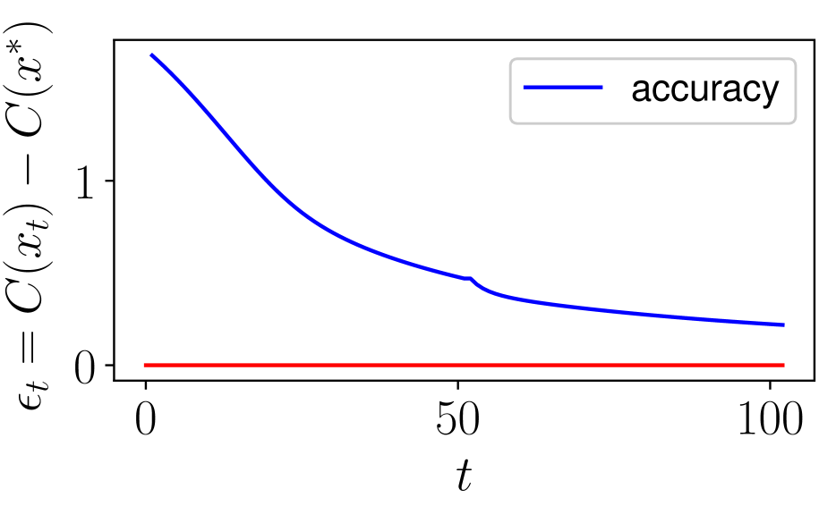
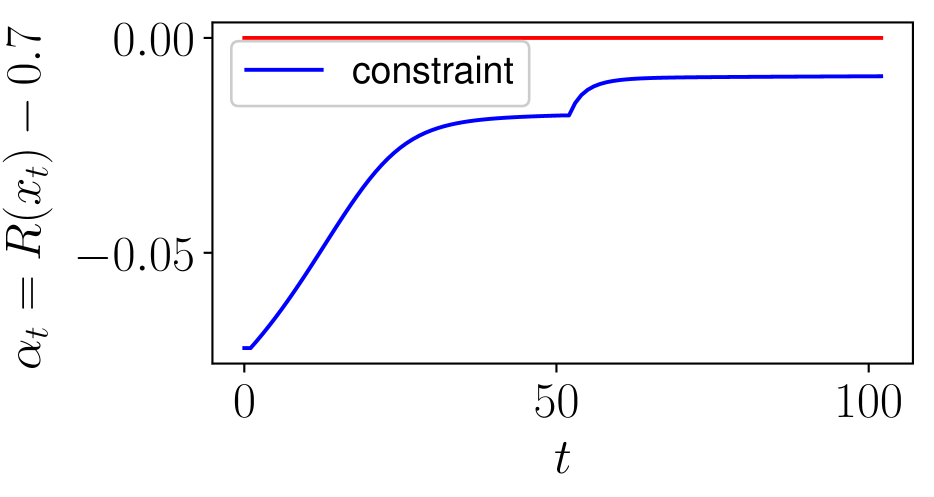
a)

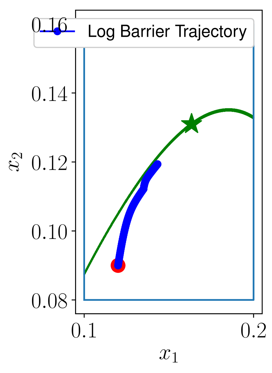
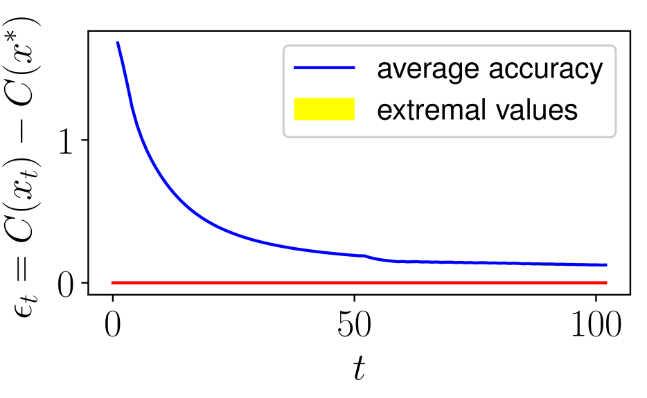
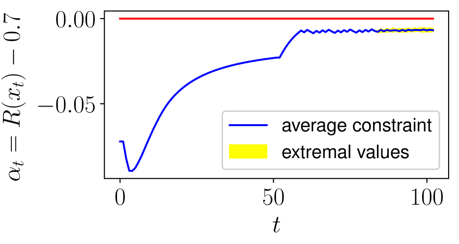
b)

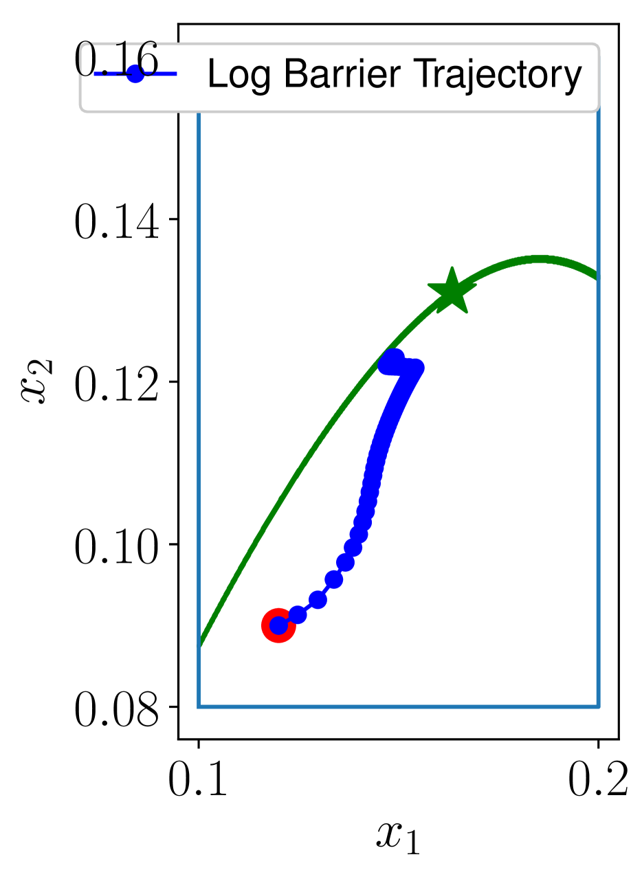
Figure 1: a) Convergence of the objective, distance to the boundary, and optimization trajectories of 0-LBM. By the green star the optimal point is denoted. Blue points denote the optimization trajectory, red point denotes the starting point, green line is the boundary $R(x)=0.7$.
b) Convergence, distance to the boundary, and optimization trajectories of s0-LBM with SZO $\xi\sim\mathcal{N}(0,\sigma^{2})$ added to the measurements $\hat{R}(x_{t},\xi)=R(x_{t})+\xi$, $\hat{C}(x_{t},\xi)=C(x_{t})+\xi$, 20 samples.

We consider the scenario of a cutting machine (Maier et al.,, 2018) which has to produce certain tools and optimize the cost of production by tuning the turning process parameters such as the feed rate $f$ and the cutting speed $\nu_{c}$. For the turning process we need to minimize a non-convex cost function $C(x)$, where the decision variable is $x=(\nu_{c},f)\in\mathbb{R}^{2}$. The constraints include box constraints and a non-convex quality roughness constraint $R(x)$. We perform realistic simulations, by using the cost function and constraints estimated from hardware experiments with artificially added normally distributed noise $\xi\sim N(0,\sigma^{2})$. The obtained non-convex smooth optimization problem with concave objective and convex constraints is:

$$\min_{x\in\mathbb{R}^{2}}\leavevmode\nobreak\ \leavevmode\nobreak\ \leavevmode\nobreak\ \leavevmode\nobreak\ \leavevmode\nobreak\ \leavevmode\nobreak\ \leavevmode\nobreak\ \leavevmode\nobreak\ \leavevmode\nobreak\ C(x)=t_{c}(x)\left(C_{M}+\frac{C_{I}}{T(x)}\right)$$

$$\text{subject to\leavevmode\nobreak\ \leavevmode\nobreak\ }R(x)\leq 0.7,x_{1}=\nu_{c}\in[100,200],$$

$$\leavevmode\nobreak\ \leavevmode\nobreak\ \leavevmode\nobreak\ \leavevmode\nobreak\ \leavevmode\nobreak\ \leavevmode\nobreak\ \leavevmode\nobreak\ \leavevmode\nobreak\ \leavevmode\nobreak\ \leavevmode\nobreak\ \leavevmode\nobreak\ \leavevmode\nobreak\ \leavevmode\nobreak\ \leavevmode\nobreak\ \leavevmode\nobreak\ \leavevmode\nobreak\ \leavevmode\nobreak\ \leavevmode\nobreak\ \leavevmode\nobreak\ \leavevmode\nobreak\ \leavevmode\nobreak\ \leavevmode\nobreak\ \leavevmode\nobreak\ \leavevmode\nobreak\ \leavevmode\nobreak\ \leavevmode\nobreak\ \leavevmode\nobreak\ \leavevmode\nobreak\ \leavevmode\nobreak\ \leavevmode\nobreak\ \leavevmode\nobreak\ \leavevmode\nobreak\ x_{2}=f\in[0.08,0.16].$$

Here $t_{c}(x)=\frac{LD\pi}{\nu_{c}f},$ $T(x)=127.5365-0.84629\nu_{c}-144.21f+0.001703\nu_{c}^{2}+0.3656\nu_{c}f,$ $R(x)=0.7844-0.010035\nu_{c}+7.0877f+0.000034\nu_{c}^{2}-0.018969\nu_{c}f,$ $C_{I}=40$, $C_{M}=50$. Note that we assume the box constraints to be known, i.e., not corrupted with noise. However, the roughness constraint $R(x)$ and the cost $C(x)$ are assumed to be unknown and we only can measure their values. Hence, this problem is an instance of the safe learning problem formulated in (2). More details are presented by Maier et al., (2018), who proposed to use Bayesian optimization to solve the problem. Although the Bayesian optimization used there indeed requires a small number of measurements, it is not safe and hence may require several measurements to be taken in the unsafe region. The roughness constraints are not fulfilled for unsafe measurements, i.e., the tools produced during unsafe experiments could not be realised in the market. That is why safety is necessary for this problem. Although there exist safe Bayesian optimization methods, they require strong prior knowledge in terms of suitable kernel function. We solve barrier sub-problem (6) iteratively $K=2$ times using s0-LBM with decreasing $\eta_{k+1}=\frac{\eta_{k}}{\mu}$, where we fix $\mu=5$. We set $\sigma=0.01,L=7,M=5,\delta=0.01$ and re-scaled $\nu^{\prime}_{c}=0.001\nu_{c}$ so that $\nu^{\prime}_{c}\in[0.1,0.2].$ The starting point is $x_{0}=(\nu^{\prime}_{c},f)=(0.15,0.09).$ In Figure 1a) we show the performance of 0-LBM, and in b) we run 20 realizations s0-LBM. In all the realizations the method converges to a local optimum and the constraints are not violated.

7 CONCLUSION

We developed a zero-th order algorithm guaranteeing safety of the iterates and converging to a local stationary point. We provided its convergence analysis, which is comparable to existing zero-th order methods for non-convex optimization, and demonstrated its performance in a case study.

Appendix A

Proof.

First, recall that $\alpha_{t}=\min_{i=1,\ldots,m}-f^{i}(x).$ Note that $\lambda_{t}^{i}=\frac{\eta}{-f^{i}(x_{t})},$ $\|\lambda_{t}\|_{\infty}=\max_{i=1,\ldots,m}\frac{\eta}{-f^{i}(x_{t})}=\frac{\eta}{\min_{i=1,\ldots,m}-f^{i}(x_{t})}=\frac{\eta}{\alpha_{t}}.$ Recall that the steps are given by

$$x_{t+1}= x_{t}-\gamma_{t}g_{t}=x_{t}-\gamma_{t}\bigg{(}G^{0}(x_{t},\nu_{t})+\eta\sum_{i=1}^{t}\frac{G^{i}(x_{t},\nu_{t})}{-f^{i}(x_{t})}\bigg{)},$$ (19)

where the safe step size $\gamma_{t}$ is $\gamma_{t}=\min\left\{\frac{\min_{i}\{-\hat{f}_{i}(x_{t})\}}{2L\|\hat{g}_{t}\|},\frac{1}{L_{2}(x_{t})}\right\}.$ In the paper (Hinder and Ye,, 2019) the authors have shown that

$$L_{2}(x_{t}) =M\left(1+\sum_{i=1}^{m}\frac{2\eta}{\{-f^{i}(x_{t})\}}\right)+\sum_{i=1}^{m}\frac{4\eta L}{(-f^{i}(x_{t}))^{2}}=M(1+2\|\lambda_{t}\|_{1})+\frac{4L\|\lambda_{t}\|_{2}^{2}}{\eta}$$

represents a "local" Lipschitz constant of $\nabla B_{\eta}(x)$ at the point $x_{t}$. In particular in Lemma 1(Hinder and Ye,, 2019) the authors have shown that $|v^{T}\nabla^{2}B_{\eta}(x_{t}+\theta v)v|\leq L_{2}(x_{t})$ for any $\theta\leq\frac{\alpha_{t}}{2L}$ and $v\in B(0,1)$. Note that

$$L_{2}(x_{t}) =M\left(1+\sum_{i=1}^{m}\frac{2\eta}{\{-f^{i}(x_{t})\}}\right)+\sum_{i=1}^{m}\frac{4\eta L^{2}}{(-f^{i}(x_{t}))^{2}}=M(1+2\|\lambda_{t}\|_{1})+\frac{4L^{2}\|\lambda_{t}\|_{2}^{2}}{\eta}$$

$$\leq M\left(1+2\frac{m\eta}{\alpha_{t}}\right)+\frac{4L^{2}\eta m}{\alpha_{t}^{2}}=M\left(1+2m\|\lambda_{t}\|_{\infty}\right)+\frac{4L^{2}m\|\lambda_{t}\|_{\infty}^{2}}{\eta}.$$

For the next inequalities we also use the fact that $\alpha_{t}=\frac{\eta}{\|\lambda_{t}\|_{\infty}}.$ Also we denote by $\hat{\gamma}_{t}=\gamma_{t}\|g_{t}\|.$ Then, at each iteration of Algorithm 1 we have

$$B_{\eta}(x_{t})-B_{\eta}(x_{t+1})\geq-\gamma_{t}\langle\nabla B_{\eta}(x_{t}),g_{t}\rangle-\frac{1}{2}L_{2}(x_{t})\gamma_{t}^{2}\|g_{t}\|^{2}_{2}=\textit{[Taylor's theorem and local smoothness]}$$

$$=\gamma_{t}\langle\zeta_{t},g_{t}\rangle+\gamma_{t}\|g_{t}\|^{2}_{2}-\frac{1}{2}L_{2}(x_{t})\gamma_{t}^{2}\|g_{t}\|^{2}_{2}\geq\textit{by definition }\gamma_{t}=\min\left\{\frac{1}{\hat{L}_{2}(x_{t})},\frac{\hat{\alpha}_{t}}{2L\|g_{t}\|}\right\}$$

$$\geq-\hat{\gamma}_{t}\|\zeta_{t}\|_{2}+\frac{{\gamma_{t}}}{2}\|g_{t}\|^{2}_{2}\geq-\hat{\gamma}_{t}\|\zeta_{t}\|_{2}+\frac{\hat{\gamma}_{t}}{2}\|g_{t}\|_{2}\geq\frac{\hat{\gamma}_{t}}{2}(\|\nabla B_{\eta}(x_{t})\|_{2}-3\|\zeta_{t}\|_{2}).$$

Hence, we can derive the following bound for all $t$ for which $\|g_{t}\|_{2}\geq\|g_{t}\|_{2}-2\|\zeta_{t}\|\geq\eta(1+\frac{\eta}{\hat{\alpha}_{t}})$, we have

$$B_{\eta}(x_{0})-\min_{x\in D}B_{\eta}(x)\geq B_{\eta}(x_{0})-B_{\eta}(x_{T})=\sum_{t=0}^{T}\left(B_{\eta}(x_{t})-B_{\eta}(x_{t+1})\right)\geq\sum_{t=1}^{T}\frac{\hat{\gamma}_{t}}{2}(\|\nabla B_{\eta}(x_{t})\|_{2}-3\|\zeta_{t}\|_{2})\geq$$

$$\geq\frac{1}{2}\sum_{t=1}^{T}\min\left\{\frac{\|g_{t}\|_{2}}{\hat{L}_{2}(x_{t})},\frac{\hat{\alpha}_{t}}{2L}\right\}\eta\left(1+\frac{\eta}{\alpha_{t}}\right)\geq\frac{1}{2}\sum_{t=1}^{T}\min\left\{\frac{\eta^{2}\left(1+\frac{\eta}{\alpha_{t}}\right)^{2}}{\hat{L}_{2}(x_{t})},\frac{\hat{\alpha}_{t}\eta\left(1+\frac{\eta}{\alpha_{t}}\right)}{2L}\right\}$$

$$\geq\frac{1}{2}\sum_{t=1}^{T}\min\left\{\frac{\eta^{2}\left(1+\frac{\eta}{\alpha_{t}}\right)^{2}}{mM\left(1+\frac{\eta}{\alpha_{t}}\right)+\frac{4L^{2}m}{\eta}(\frac{\eta^{2}}{\alpha_{t}^{2}})},\frac{\eta^{2}}{L}\right\}\geq\frac{T}{2}\min\left\{\frac{\eta^{3}}{mM\eta+4L^{2}m},\frac{\eta^{2}}{L}\right\}.$$

∎

Proof.

(Continuation) Hence after

$$T\leq 2(B_{\eta}(x_{0})-\min_{x\in D}B_{\eta}(x))\max\left\{\frac{mM\eta+4L^{2}m}{\eta^{3}},\frac{L}{\eta^{2}}\right\}.$$

iterations we will find $\|g_{k}\|_{2}-2\|\zeta_{k}\|_{2}\leq\eta\left(1+\frac{\eta}{\hat{\alpha}_{k}}\right).$ ∎

Appendix G

Proof.

For 0-LBM

$$\|\nabla B_{\eta}(x_{k})\|_{2}\leq\|g_{k}\|_{2}+\|\zeta_{k}\|_{2}\leq\eta\left(1+\frac{\eta}{\alpha_{k}}\right)+3\|\zeta_{k}\|_{2}.$$

For s0-LBM

$$\|\nabla B_{\eta}(x_{k})\|_{2}\leq\|\hat{g}_{k}\|_{2}+\|\hat{\zeta}_{k}\|_{2}\leq\eta\left(1+\frac{\eta}{\hat{\alpha}_{k}}\right)+3\|\hat{\zeta}_{k}\|_{2}\leq\eta\left(1+\frac{\eta}{\alpha_{k}}\right)+3\|\hat{\zeta}_{k}\|_{2}.$$

If $\|\zeta_{k}\|_{2}\leq\eta,$ then $\|\nabla B_{\eta}(x_{k})\|_{2}\leq\eta(4+\frac{\eta}{\hat{\alpha}_{k}}).$

$$\hat{\lambda}_{i}(-f^{i}(x_{k}))=\frac{\eta}{-\hat{f}^{i}_{\delta}(x_{k})}(-f^{i}(x_{k}))=\eta+\frac{\eta}{-\hat{f}^{i}_{\delta}(x_{k})}(\hat{f}^{i}(x_{k})-f^{i}(x_{k}))\leq\eta+\frac{\eta\varepsilon_{k}}{-\hat{f}^{i}_{\delta}(x_{k})}$$

$$\leq\eta+\frac{3\eta\nu_{k}^{2}M^{2}}{-\hat{f}^{i}_{\delta}(x_{k})}\leq\eta+3\eta\nu_{k}M\leq 4\eta.$$

Then

$$\|\nabla B_{\eta}(x_{k})\|\leq\eta(4+\|\hat{\lambda}_{k}\|_{\infty}),$$

$$\hat{\lambda}_{k}^{i}(-f^{i}(x_{t}))\leq 4\eta,$$

$$-f^{i}(x_{t}),\hat{\lambda}_{k}^{i}\geq 0,$$

i.e., $(x_{k},\hat{\lambda}_{k})$ is a $4\eta$-approximate scaled KKT point. ∎

Appendix E

Proof.

Let us denote by

$$g^{\prime}_{t}=\hat{G}^{0}(x_{t},\nu_{t},\xi)+\eta\sum_{i=1}^{m}\frac{\hat{G}^{i}(x_{t},\nu_{t},\xi)}{-f^{i}(x_{t})}$$

and $\zeta^{\prime}_{t}=g^{\prime}_{t}-\nabla B_{\eta}(x_{t}).$ Note that by Equation 14 we have $0\leq\hat{f}^{i}(x)-f^{i}(x)\leq\varepsilon_{t}$ with high probability by construction. Then, based on (15), with probability $\geq 1-\delta$

$$\|\hat{\zeta}_{t}\|_{2} =\|\hat{g}_{t}-\nabla B_{\eta}(x_{t})\|_{2}\leq\|\hat{g}_{t}-g^{\prime}_{t}\|_{2}+\|g^{\prime}_{t}-\nabla B_{\eta}(x_{t})\|_{2}$$

$$=\eta\left\|\sum_{i=1}^{m}\hat{G}^{i}(x_{t},\nu_{t},\xi)\left(\frac{1}{-\hat{f}^{i}(x_{t})}-\frac{1}{-f^{i}(x_{t},)}\right)\right\|_{2}+\|\zeta^{\prime}_{t}\|_{2}$$

$$\leq\eta\left\|\sum_{i=1}^{m}\frac{\hat{G}^{i}(x_{t},\nu_{t},\xi)}{-f^{i}(x_{t})}\frac{\varepsilon_{t}}{-\hat{f}^{i}(x_{t})}\right\|_{2}+\|\zeta^{\prime}_{t}\|_{2}\leq\frac{\eta}{\alpha_{t}\hat{\alpha}_{t}}\left\|\sum_{i=1}^{m}(\nabla f^{i}(x_{t})+\hat{\Delta}^{i}_{t})\varepsilon_{t}\right\|_{2}+\|\zeta^{\prime}_{t}\|_{2}$$

$$\leq\frac{\eta}{\hat{\alpha}_{t}^{2}}\left(mL+\sum_{i=1}^{m}\|\hat{\Delta}^{i}_{t}\|_{2}\right)\varepsilon_{t}+\sqrt{\|\hat{\Delta}^{0}_{t}\|^{2}_{2}+\sum_{i=1}^{m}\frac{\eta^{2}}{\alpha_{t}^{2}}\|\hat{\Delta}^{i}_{t}\|^{2}_{2}}$$

Recall that by Lemma 1 with probability $\geq 1-\delta$, if $n_{t}=\frac{8\sigma^{2}\ln\frac{1}{\delta}}{3M^{2}\nu_{t}^{4}}.$

$$\|\hat{\Delta}_{t}\|^{2}_{2}\leq\frac{d\nu_{t}^{2}M^{2}}{4}+2d\sigma^{2}\frac{\ln 1/\delta}{n_{t}\nu_{t}^{2}}\leq d\nu_{t}^{2}M^{2}$$

$$\varepsilon_{t}\leq 2\frac{\sigma\sqrt{\ln\frac{1}{\delta}}}{\sqrt{n_{t}}}\leq M\nu_{t}^{2}$$

Then

$$\|\hat{\zeta}_{t}\|_{2} \leq\frac{\eta}{\hat{\alpha}_{t}^{2}}M\nu_{t}^{2}\left(mL+m\sqrt{d}\nu_{t}M\right)+\sqrt{d\nu_{t}^{2}M^{2}+m\frac{\eta^{2}}{\alpha_{t}^{2}}d\nu_{t}^{2}M^{2}}.$$

If $\nu_{t}=\min\{\frac{\eta}{\sqrt{d}M},\frac{\alpha_{t}}{L},\frac{\alpha_{t}}{m\sqrt{d}M}\}$, then

$$\mathbb{P}\bigg{\{}\|\hat{\zeta}_{t}\|_{2}\leq\eta\left(4+\frac{\eta}{L\sqrt{d}}\right)\bigg{\}}\geq 1-\delta.$$ (20)

∎

Appendix F

Proof.

Denote by $\xi^{i}_{t,j}:=\frac{\sum_{l=1}^{n_{t}}\xi^{i}_{jl}}{n_{t}}$ at iteration $t$. The deviation is bounded as follows.

$$\|\hat{\Delta}_{t}^{i}\|_{2}=\|\hat{G}^{i}(x_{t},\nu_{t},\xi^{i}_{(n_{t})})-\nabla f^{i}(x_{t})\| =\sqrt{\sum_{j=1}^{d}\left[\frac{f^{i}(x_{t}+\nu_{t}e_{j})+\xi^{i}_{t,j}-f^{i}(x_{t})-\xi^{i}_{t,0}}{\nu_{t}}-\langle\nabla f^{i}(x_{t}),e_{j}\rangle\right]^{2}\|e_{j}\|^{2}}\leq$$

$$\leq\sqrt{\frac{d\nu^{2}M^{2}}{4}+\frac{1}{\nu_{t}^{2}}\sum_{j=1}^{d}[\xi^{i}_{t,j}-\xi^{i}_{t,0}]^{2}}\leq\sqrt{\frac{d\nu_{t}^{2}M^{2}}{4}+\frac{1}{\nu_{t}^{2}}\sum_{j=1}^{d}[\xi^{i}_{t,j}-\xi^{i}_{t,0}]^{2}}$$

Hence, the deviation is upper bounded with high probability by

$$\mathbb{P}\left\{\|\hat{\Delta}_{t}^{i}\|_{2}\leq\sqrt{\frac{d\nu_{t}^{2}M^{2}}{4}+2d\sigma^{2}\frac{\ln 1/\delta}{n_{t}\nu_{t}^{2}}}\right\}\geq 1-\delta$$

Hence, $n_{t}$ has to be chosen by trading off this 2 terms. Setting $n_{t}\geq\frac{8\sigma^{2}\ln\frac{1}{\delta}}{3\nu_{t}^{4}M^{2}}$, we obtain:

$$\mathbb{P}\left\{\|\hat{\Delta}_{t}^{i}\|_{2}\leq\sqrt{d}\nu_{t}M\right\}\geq 1-\delta$$ (21)

∎

Appendix D

Proof.

Recall $\xi^{i}_{t,j}:=\frac{\sum_{l=1}^{n_{t}}\xi^{i}_{jl}}{n_{t}}.$ Note that

$$f^{i}(x_{t})=F^{i}(x_{t},\xi^{i}_{t,0})-\xi^{i}_{t,0}=\frac{1}{n_{t}}\sum_{l=1}^{n_{t}}F^{i}(x_{t},\xi^{i}_{0l})-\frac{1}{n_{t}}\sum_{l=1}^{n_{t}}\xi^{i}_{0l}$$

From the sub-Gaussian property of $\xi^{i}_{0}$ and Hoeffding inequality, we have that:

$$\mathbb{P}\left\{\sum_{l=1}^{n_{t}}\frac{\xi^{i}_{0l}-\mathbb{E}\xi^{i}_{0l}}{n_{t}}\geq b\right\}=\mathbb{P}\left\{\frac{1}{n_{t}}\sum_{l=1}^{n_{t}}\xi^{i}_{0l}\geq b\right\}\leq\exp{\frac{-n_{t}b^{2}}{\sigma^{2}}}=\delta.$$

Then $b=\frac{\sigma\sqrt{\ln\frac{1}{\delta}}}{\sqrt{n_{t}}},$ $\mathbb{P}\left\{\frac{1}{n_{t}}\sum_{l=1}^{n_{t}}\xi^{i}_{0l}\leq\frac{\sigma\sqrt{\ln\frac{1}{\delta}}}{\sqrt{n_{t}}}\right\}\geq 1-\delta.$ Similarly,

$$\mathbb{P}\left\{\frac{1}{n_{t}}\sum_{l=1}^{n_{t}}-\xi^{i}_{0l}\leq\frac{\sigma\sqrt{\ln\frac{1}{\delta}}}{\sqrt{n_{t}}}\right\}\geq 1-\delta.$$

Hence, if $\hat{f}^{i}_{\delta}=\frac{1}{n_{t}}\sum_{l=1}^{n_{t}}F^{i}(x_{t},\xi^{i}_{0l})+\frac{\sigma\sqrt{\ln\frac{1}{\delta}}}{\sqrt{n_{t}}},$ then $\mathbb{P}\left\{\hat{f}^{i}_{\delta}-2\frac{\sigma\sqrt{\ln\frac{1}{\delta}}}{\sqrt{n_{t}}}\leq f^{i}_{\delta}\leq\hat{f}^{i}_{\delta}\right\}\geq 1-\delta.$ ∎

Appendix H.

Proof.

Assume we have only one smooth constraint $f^{1}(x)$, $m=1$. Also, assume that close enough to the boundary $\forall x\in D:f^{1}(x)\geq-\eta$ we have $\|\nabla f^{1}(x)\|\geq F.$
Assume that for some $x_{t}$ $-f^{1}(x_{t})\leq\frac{F^{2}}{L^{2}+\eta}\eta.$ At that point

$$F\leq\|\nabla f^{1}(x_{t})\|\leq L$$

and

$$\|\nabla f^{1}(x_{t})\|\leq L$$

Then the step direction $-\hat{g}_{t}=-\nabla B_{\eta}+\hat{\zeta}_{t}$ is such that

$$\langle\hat{g}_{t},\nabla f^{1}(x_{t})\rangle=\langle\nabla B_{\eta}+\hat{\zeta}_{t},\nabla f^{1}(x_{t})\rangle=$$

$$\langle\nabla f^{0}(x_{t})+\eta\frac{\nabla f^{1}(x_{t})}{-f^{1}(x_{t})}+\hat{\zeta}_{t},\nabla f^{1}(x_{t})\rangle\geq\langle\nabla f^{0}(x_{t}),\nabla f^{1}(x_{t})\rangle+\frac{\|\nabla f^{1}(x_{t})\|^{2}}{F^{2}/(L^{2}+\eta L)}-\eta L\geq L^{2}+\eta L-L^{2}-\eta L\geq 0.$$

Then if $\gamma_{t}\leq\frac{1}{M}$ and $-f^{1}(x_{t})\leq\frac{F^{2}}{(L^{2}+\eta L)}\eta$, the next step $f^{1}(x_{t+1})<f^{1}(x_{t})$ will decrease. On the other hand, if $-f^{1}(x_{t})\geq\frac{F^{2}}{(L^{2}+\eta L)}\eta$ for one step it cannot decrease more than twice $f^{1}(x_{t+1})\geq\frac{F^{2}}{2(L^{2}+\eta L)}\eta.$ Hence, for $x_{t}$ generated by s0-LBM we can guarantee $-f^{1}(x_{t})\geq\frac{F^{2}}{2(L^{2}+\eta L)}\eta.$ ∎

Appendix I.

Proof.

Using smoothness

$$f(x)\geq f(y)+\langle\nabla f(y),x-y\rangle-\frac{M}{2}\|x-y\|_{2}^{2}$$

we can obtain

$$\|\Delta_{t}^{i}\|_{2} =\sqrt{\sum_{j=1}^{d}\left[\frac{f^{i}(x_{t}+\nu_{t}e_{j})-f^{i}(x_{t})}{\nu_{t}}-\langle\nabla f^{i}(x_{t}),e_{j}\rangle\right]^{2}\|e_{j}\|_{2}^{2}}$$

$$\leq\sqrt{\sum_{j=1}^{d}\left[\frac{f^{i}(x_{t}+\nu_{t}e_{j})-f^{i}(x_{t})-\langle\nabla f^{i}(x_{t}),\nu_{t}e_{j}\rangle}{\nu_{t}}\right]^{2}\|e_{j}\|_{2}^{2}}$$

$$\leq\sqrt{\sum_{j=1}^{d}\left[\frac{M\nu_{t}^{2}}{2\nu_{t}}\right]^{2}}\leq\frac{\sqrt{d}\nu_{t}M}{2}.$$

∎

References

- Bach and Perchet, (2016) Bach, F. and Perchet, V. (2016). Highly-smooth zero-th order online optimization. In Conference on Learning Theory, pages 257–283.
- Balasubramanian and Ghadimi, (2018) Balasubramanian, K. and Ghadimi, S. (2018). Zeroth-order (non)-convex stochastic optimization via conditional gradient and gradient updates. In Advances in Neural Information Processing Systems, pages 3455–3464.
- Berkenkamp et al., (2016) Berkenkamp, F., Krause, A., and Schoellig, A. P. (2016). Bayesian optimization with safety constraints: safe and automatic parameter tuning in robotics. arXiv preprint arXiv:1602.04450.
- Birgin et al., (2016) Birgin, E. G., Gardenghi, J., Martinez, J. M., Santos, S. A., and Toint, P. L. (2016). Evaluation complexity for nonlinear constrained optimization using unscaled kkt conditions and high-order models. SIAM Journal on Optimization, 26(2):951–967.
- Carmon et al., (2017) Carmon, Y., Duchi, J. C., Hinder, O., and Sidford, A. (2017). Lower bounds for finding stationary points i. Mathematical Programming, pages 1–50.
- Cartis et al., (2014) Cartis, C., Gould, N. I., and Toint, P. L. (2014). On the complexity of finding first-order critical points in constrained nonlinear optimization. Mathematical Programming, 144(1-2):93–106.
- Facchinei et al., (2017) Facchinei, F., Lampariello, L., and Scutari, G. (2017). Feasible methods for nonconvex nonsmooth problems with applications in green communications. Mathematical Programming, 164(1-2):55–90.
- Ghadimi and Lan, (2013) Ghadimi, S. and Lan, G. (2013). Stochastic first-and zeroth-order methods for nonconvex stochastic programming. SIAM Journal on Optimization, 23(4):2341–2368.
- Hinder and Ye, (2018) Hinder, O. and Ye, Y. (2018). A one-phase interior point method for nonconvex optimization. arXiv preprint arXiv:1801.03072.
- Hinder and Ye, (2019) Hinder, O. and Ye, Y. (2019). A polynomial time log barrier method for problems with nonconvex constraints. arXiv preprint: https://arxiv.org/pdf/1807.00404.pdf.
- Maier et al., (2018) Maier, M., Rupenyan, A., Zwicker, R., Akbari, M., and Wegener, K. (2018). Turning: Autonomous process set-up through bayesian optimization and gaussian process models in turning. 12th CIRP Conference on Intelligent Computation in Manufacturing Engineering, Gulf of Naples, Italy.
- Schaal and Atkeson, (2010) Schaal, S. and Atkeson, C. G. (2010). Learning control in robotics. IEEE Robotics & Automation Magazine, 17(2):20–29.
- Sui et al., (2015) Sui, Y., Gotovos, A., Burdick, J., and Krause, A. (2015). Safe exploration for optimization with gaussian processes. In International Conference on Machine Learning, pages 997–1005.
- Tang et al., (2014) Tang, C.-m., Liu, S., Jian, J.-b., and Li, J.-l. (2014). A feasible sqp-gs algorithm for nonconvex, nonsmooth constrained optimization. Numerical Algorithms, 65(1):1–22.
- Topkis and Veinott, (1967) Topkis, D. M. and Veinott, Jr, A. F. (1967). On the convergence of some feasible direction algorithms for nonlinear programming. SIAM Journal on Control, 5(2):268–279.
- Usmanova et al., (2019) Usmanova, I., Krause, A., and Kamgarpour, M. (2019). Safe convex learning under uncertain constraints. In The 22nd International Conference on Artificial Intelligence and Statistics, pages 2106–2114.
- Yu and Ho, (2019) Yu, Z. and Ho, D. W. (2019). Zeroth-order stochastic block coordinate type methods for nonconvex optimization. arXiv preprint arXiv:1906.05527.