A schematic reaction-theory model for nuclear fission

Abstract

The K-matrix formalism is applied to a schematic model for nuclear fission. The purpose is to explore the dependence of observables on the assumptions made about the configuration space and nucleon interaction in the Hamiltonian of the fissile nucleus. As expected, branching ratios in induced fission are found to depend sensitively on the character of the residual interaction, whether it is pairing in form or taken from a random ensemble. On the other hand, the branching ratio is not much affected by the presence of additional configurations that do not introduce new fission paths.

I Motivation

Nuclear fission is one of the most challenging topics in the quantum theory of finite many-particle systems. Useful phenomenological models are available that take into account both nuclide-dependent shell effects and nucleon-blind collective variables, see sch16 ; sch18 for recent reviews. But anchoring these models to the underlying many-body Hamiltonian faces enormous obstacles related to the huge number of many-body configurations participating in the dynamics.

It is obvious that the practical theory should be informed by microscopic Hamiltonian dynamics, but since a full Hamiltonian theory is presently out of reach, it might be useful to examine simple models that include qualitative aspects of the complete Hamiltonian. Perhaps the reliability of the various approximation schemes can be assessed in much smaller spaces than would be required for a quantitative theory. It is the goal of the present work to propose a simplified model for this purpose.

Most fission theory based on nucleonic Hamiltonians is carried out in the time domain, for example with time-dependent mean field approximationssim18 ; bul15 . In contrast, the physical observables in fission reactions are the energy-dependent cross sections. This is another reason for using reaction theory in constructing models.

II Reaction theory

The K-matrix formalism is well-suited for a Hamiltonian-based reaction theory of multi-particle systems. It has been used in a number of different branches of physicsdal61 ; chu95 ; fyo96 ; alh00 ; lin19 . In nuclear physics, it has been applied nucleon-induced reactions using Hamiltonians based on nucleon-nucleon interactionmah69 . It has also been successfully applied to develop statistical reaction theorymit10 ; kaw15 . The $K$-matrix formalism is built on two matrix components. The first is a Hamiltonian matrix $H$ in the space of internal or quasi-bound configurations. Some of these configurations have decay amplitudes to possible final-state channels. These amplitudes are contained in a second matrix ${\tilde{\gamma}}$. It has $N_{conf}$ rows corresponding to the dimension of $H$ and $N_{ch}$ columns corresponding to the number of decay channels. The $K$-matrix is defined as

$$K=\pi{{\tilde{\gamma}}}^{T}\frac{1}{E-H}{{\tilde{\gamma}}}$$ (1)

where $E$ is the total energy of the reacting system. The $S$-matrix is computed as

$$S=\frac{1-iK}{1+iK}.$$ (2)

The partial width $\gamma_{\mu c}$ for a configuration $\mu$ decaying through channel $c$ is

$$\Gamma_{\mu c}=2\pi\gamma^{2}_{\mu c}.$$ (3)

Eq. (1) effectively separates the computational problem into separate tasks. The first task is the construction of a Hamiltonian matrix $H$ for the internal states. It requires setting up a basis composed of many-body configurations and computing the interactions between the configurations. This configuration-interaction (CI) approach is very well known, and it has been very successful in many fields including nuclear structure physics. The second task is to calculate ${\tilde{\gamma}}$, the matrix of partial decay widths of the internal states to the continuum channels. This is much more challenging when the channel states are all composite particles; at this point the needed approximations are not testable with simple models ber19 . Given the two matrices, all that remains of the computation is ordinary linear algebra.

III Model Hamiltonian

The requirements for the model Hamiltonian are that it:
–is expressible in terms of one- and two-body Fock-space operators;
–defines an operator $\hat{Q}$ that can be used to measure the evolving shape of the fissioning system;
–is flexible enough to simulate induced fission as well as spontaneous fission.

These requirements can be fulfilled by the following model. Configurations are generated in a space of $N_{orb}$ orbitals, each orbital containing two time-reversed pairs $k$ and $\bar{k}$. The first $N_{orb}/2$ orbitals are fully occupied in the ground-state configuration, while the remaining $N_{orb}/2$ orbitals are fully occupied in the doorway state to fission. In operator representation, the Hamiltonian is

$$\hat{H}=\sum_{k=1}^{N_{orb}/2}\left((k\;\mathrm{mod}\;N_{orb}/2)-1\right)\varepsilon_{0}\hat{n}_{k}+v_{Q}\hat{Q}\hat{Q}+\sum_{k,k^{\prime}}v_{k,k^{\prime}}\hat{P}^{\dagger}_{k}\hat{P}_{k^{\prime}}.$$ (4)

Here $\hat{n}_{k}=\hat{a}^{\dagger}_{k}\hat{a}_{k}+\hat{a}^{\dagger}_{\bar{k}}\hat{a}_{\bar{k}}$ gives the occupation number of the $k$ orbital, $\hat{P}^{\dagger}_{k}=\hat{a}^{\dagger}_{k}\hat{a}^{\dagger}_{\bar{k}}$ is the pair creation operator, and $\hat{Q}=\sum_{k}q\hat{n}_{k}$ measures the elongation of the configuration. In the expression for $\hat{Q}$ $q(k)=\pm 1$ for the first $N_{orb/2}/2$ orbitals and $-1$ for the others. Note that the first two terms in $\hat{H}$ are diagonal in the configurations and serve to define their energies.

The qualitative scheme of orbital energies and how they are filled for low-energy configurations is shown in Fig. 1, assuming the parameter $v_{Q}$ in the Hamiltonian is negative.

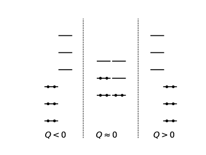
Figure 1: Single-particle spectra at different deformations, taking $v_{Q}<0$ in the model Hamiltonian. The orbital occupancies of low-energy configurations are indicated by the filled circles.

The left-hand configuration has all $q=-1$ orbitals filled and represents the ground state of the fissile nucleus. The one on the right with all $q=+1$ orbitals filled represents a scission doorway configuration.

For the numerical calculations we take $N_{orb}=6$ for the dimension of the orbital space. The space is half filled with $N=6$ nucleons that occupy the orbitals as pairs. The configurations are thus restricted to seniority zero; the dimension of the space is

$$N_{conf}={6\choose 3}=20.$$ (5)

$Q$ in the model ranges from -6 to +6, with one state at each end point and 18 states in between. As an example, Fig. 2

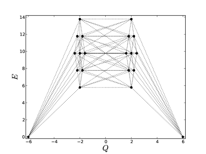
Figure 2: Spectrum of the barrier model. The vertical axis has been shifted to put the entry and prescission configurations at zero energy. The horizontal positions of the configurations have been slightly shifted to make visible the degeneracies of the intermediate configurations. The dotted lines join configurations that are connected by $v_{k,k^{\prime}}$.

shows the energy of the configurations as a function of $Q$ in the ”barrier” model, constructed with $v_{Q}=-\frac{1}{4}e_{0}$. The Figure also shows the connectivity of the network linked by the two-particle interaction. The state at $Q=-6$ will be coupled to an entrance channel, and the one at $Q=+6$ will be coupled to a fission channel. With the energies of the configurations as depicted in Fig. 2, the model could simulate the fission cross section in the presence of a barrier along the fission path. Note that $Q$ is a discrete property of individual configurations. This is to be contrasted with the generator-coordinate method (GCM) of constrained Hartree-Fock theoryben03 which treats the expectation value $\langle Q\rangle$ as a continuous variable.

For the present study we will examine the fission-to-capture branching ratio at energies above the barriers. Physically, the level density of internal states is very large. In the model with $V_{Q}=0$, the highest level density of the internal states is at the entry doorway energy. The resulting configuration energies are shown in Fig. 3; we shall call this the “no-barrier” model. Note that the fission doorway energy is also at the point of highest level density.

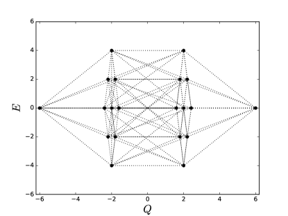
Figure 3: Spectrum of the ”no barrier” Hamiltonian. The vertical axis has shifted to put the first and last configurations at zero energy.

Two extreme choices for the interaction will be examined. The first is the pure pairing model,

$$v_{k,k^{\prime}}=-G\,\,\,\,\,\,{\rm(pairing)}$$ (6)

where $G$ is the pairing strength. The other extreme is a random interaction taken from a Gaussian ensemble. Here the probability $W$ of the interaction strength $v_{k,k^{\prime}}$ is taken as

$$W(v_{k,k^{\prime}})=\frac{1}{\sqrt{2\pi G^{2}}}\exp(-v_{k,k^{\prime}}^{2}/2G^{2})\,\,\,\,\,\,{\rm(random)}.$$ (7)

The two model interactions have equal rms matrix elements.

There is a technical problem in using the Hamiltonian as given for the pairing interaction. Namely, the uniform spacing of the single-particle energies produces a significant degeneracy in the energies of the configurations. This might give rise to unphysical effects in the transport properties of the Hamiltonian. This problem is mitigated in the numerical calculations by modifying the single-particle energies to

$$\varepsilon_{k}^{\prime}=\varepsilon_{k}+0.1r_{k}e_{0}.$$ (8)

Here $r_{k}$ is a random number of unit variance taken from a Gaussian ensemble. In fact this complication of the model is physically warranted: the spacings are also not uniform in more realistic models. The cost of introducing random terms into the Hamiltonian is that the ensemble must be sampled multiple times to compute observables.

The two-particle interaction strength is the last parameter in the Hamiltonian that needs to be set. Here one can get guidance from empirical pairing systematics. The mixing between low-lying Hartree-Fock configurations is controlled by the ratio of pairing gap $\Delta$ and the average level spacing $e_{0}$ of the single-particle orbitals. In actinide nuclei, the (neutron) pairing gap is about

$$\Delta\approx 12./A^{1/2}\approx 0.75\;\;\mathrm{MeV}.$$ (9)

The neutron orbital spacing roughly given in terms of the number of neutrons $N$ in the nucleus and their kinetic energy at the Fermi surface $\varepsilon_{f}$ as

$$e_{0}\approx\frac{4\varepsilon_{f}}{3N}\approx 0.33\;\;\mathrm{MeV}.$$ (10)

This yields a ratio $\Delta/\varepsilon_{0}\approx 2.25$. This is close to the calculated ratio for the barrier model taking the pairing strength to be $G=e_{0}$; this value is adopted for numerical computation in the following section. Table 1 summarizes the numerical parameters for the no-barrier model.

Parameter	Value
$N_{orb}$	6
$N$	6
$v_{Q}$	0
$G$	1

Table 1: Parameters for the model Hamiltonian. Energies are in units of $e_{0}$.

IV Application to branching ratios

In this section the model is applied to the fission-to-capture branching ratio. To treat this as a reaction in the K-matrix theory, we need to assign partial widths for the entrance, capture, and fission channels. For a fissile nucleus such as ²³⁵U bombarded with low-energy neutrons, the fission and capture widths are comparable, and the entrance channel width is small compared to both of them. This is achieved by the partial widths assignments shown in Table II.

Configuration $\mu$	Channel	$\Gamma_{\mu,c}/e_{0}$
$1$	n	$0.063$
$1$	c	$1.0$
$20$	f	$1.0$

Table 2: Partial widths for modeling the fission-to-capture branching ratio. Channel labels are: $n$ for entry channel as in neutron-induced fission; $c$ capture leading to the ground state of the fissile nucleus; $f$ fission decay.

We can now apply the $K$-matrix formula to calculate the $S$-matrix elements for the three channels. The cross sections show large fluctuations associated with individual resonances in the internal structure of the fissioning nucleus. This may be seen in Fig. 3 and 4, plotting the strengths $|S_{nc}|^{2}$ and $|S_{nf}|^{2}$ as a function of energy.

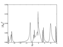
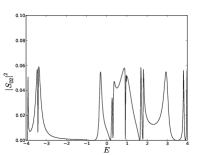
Figure 4: $S$-matrix transmission strengths for the pairing Hamiltonian. Upper panel: $|S_{01}|^{2}$; lower panel: $|S_{02}|^{2}$.

The branching ratios are highly fluctuating quantities as a function of energy, so we only report averages. The fission-to-capture ratio is calculated as

$$\alpha^{-1}=\frac{\langle|S_{nf}|^{2}\rangle}{\langle|S_{nc}|^{2}\rangle},$$ (11)

where the brackets denote an energy average. We have taken a window of energies from $E=-4\varepsilon_{0}$ to $E=4\varepsilon_{0}$ for making the averages. The results are shown in Table III under the column $\alpha^{-1}$.

$N_{conf}$	$v_{k,k^{\prime}}$	$\alpha^{-1}$
20	pairing	$0.82\pm 0.06$
20	random	$0.28\pm 0.13$
20+18	pairing	$0.73\pm 0.05$
20+18	random	$0.28\pm 0.12$

Table 3: Branching ratio $\alpha^{-1}$ for the parameter treatments discussed in the text.

The first entry in the Table uses the pairing Hamiltonian following Eq. (4), (6) and (7). The branching between capture and fission is close to one for the chosen parameters. This is just what one expects in the naïve compound nucleus model, since the Hamiltonian has equal couplings to neutron capture and fission. However, from the perspective of transport theory one would have expected the branching to the exit channel from the entry doorway would be much favored. That turns out to be the case when the random interaction is used in the model, as may be seen in the second line of Table III. There the calculated branching ratio is a factor three smaller than the pairing or compound nucleus models. Clearly, the coherence of the pairing interaction has a major effect on branching ratios between different decay modes. While that qualitative conclusion does not come as a surprise, the model shows that the means to study such issues are at hand, given an adequate basis of configurations and their couplings to decay channels.

We would also like to see the effects of the severe model space truncation. It is easy to add configurations that couple to the ones in the Hamiltonian but do not change the deformation $Q$; these may be called “spectator” configurations. The bottom two lines in Table III show the results for augmenting the space by adding 18 spectator states, each one coupled to a non-doorway state of the Hamiltonian depicted in Fig. 3. As may be seen in Table III, the resulting branching ratio for both interactions is hardly changed or not changed at all. This is good news for justifying the drastic truncations of the configuration spaces needed in more realistic models. However, it is somewhat puzzling that models that couple collective variables to internal degrees of freedom, eg. Ref. cal83 ; sca15 , show significant effects in time-dependent dynamics. It may be that branching ratios are nevertheless insensitive to spectator configurations, or it might be that the present size of the model space is too small to see a real effect.

V Extensions of the model

To make firm conclusions about the approximations invoked in realistic fission theory, it is essential to include both neutron and protons in the Hamiltonian. To this end, one can easily generalize Eq. (4) to include both species of particles, allowing them to interact with each other through the field $\hat{Q}$. The dimension of the space as constructed in Sect. (II) increases from $N_{conf}=20$ to $20^{2}=400$. The resulting model has a small enough dimension to permit easy coding and quick execution times on laptop computers. One should not expect qualitative differences in the comparisons that were presented with the present model. The changes in the proton shape distributions will track closely with the neutrons, and the separate coherences of the two pairing fields will preserve and perhaps amplify the stronger transport through shape changes.

More challenging for a more realistic model is to extend the space beyond seniority zero to access quasiparticle excitations. The statistical properties such as level densities depend crucially on these excitations. In models of fission such as the Langevin dynamics, the quasiparticles provide a thermal reservoir for energy exchanges with the collective degrees of freedom. In the context of the present model, the dimension of the space (for one species) goes from 20 to

$${12\choose 6}=924.$$ (12)

Including both protons and neutrons, the total dimension becomes $\approx 10^{6}$. The resulting computational problem is then well beyond the capabilities of general-purpose linear algebra libraries and laptop computers. Aside from the numerical challenge, it is far from clear how to parameterize the interaction Hamiltonian between quasiparticles. It is easy to model the pairing interaction and the $Q$-dependent mean-field interaction, but interactions that change the number of quasiparticles or scatter them from one set of orbitals to another are not well understood.

A nice feature of CI models of induced fission is that the same Hamiltonian can also be applied to spontaneous fission. The physical observable for spontaneous fission is the lifetime or the decay rate. To calculate the decay widths, one simply adds partial fission widths $i\Gamma_{muf}/2$ to the diagonal energies of the fission doorway state and diagonalizes the resulting non-Hermitian Hamiltonian. The mean lifetime of the ground state is then given by $\tau=\hbar/2{\rm Im}E_{gs}$. The tunneling physics is be simulated by adjusting $v_{Q}$ to make a barrier between the leftmost configuration and the fission doorway on the right, as shown in Fig. 2.

For completeness, it should be mentioned that an important quantity for reaction theory in a statistical regime is the channel transmission coefficient $T_{c}$. This may be defined empirically as $T_{c}=1-R_{c}$ where $R_{c}$ is the average reflection probability for an incoming flux in the channel $c$. The averaging makes sense only if there are many doorways to the channel; if that is the case and the average partial decay width is small, the transmission factor can be calculates as

$$T_{c}=2\pi\frac{\langle\Gamma_{\mu c}\rangle}{D}$$ (13)

where $D$ is the average level spacing the doorways. Obviously, transmission coefficients are beyond the scope of the present model since it has only one doorway for each decay model. Whether an extension of the model to many doorways can be achieved with parameters justified by a nucleonic Hamiltonian remains to be seen.

VI Summary

In a general sense, the subject of this work was a simplified model of large-amplitude shape changes in a fermionic system. The model can only be solved numerically, but the dimension is small enough to carry out with desktop tools. The first finding is confirmation of the accepted wisdom that the pairing interaction plays a major role in nuclear fission, although it was not so evident in previous models of induced fission. With enough excitation energy, the coherence of the pairing interaction should disappear and the observables should be close to those calculated with the random interaction. It would be of interest see what the energy limits are and how they correlate with the collapse of the pairing condensate at finite temperature.

Another provocative finding concerns the role of spectator configurations. The naïve expectation is not borne out that these configurations would decrease the branching ratio of fission to capture because they would slow down the dynamic evolution. According to the model, that effect is quite small. Whether it remains small in larger and more realistic model spaces is another interesting open question.

VII Acknowledgments

I would like to thank J. Dobaczewski, K. Hagino, W. Nazarewicz, and other participants in the workshop ”Future of Fission Theory”, York, UK (2019) for discussions motivating this work.

References

- (1) N. Schunck and L.M. Robledo, Rep. Rog. Phys. 79 116301 (2016).
- (2) K.H. Schmidt and Beatriz Jurado, Rep. Rog. Phys. 81 106301 (2018).
- (3) C. Simenel and A.S. Umar, Prog. Part. Nucl. Phys. 100 19 (2018).
- (4) A. Bulgac, P. Magierski, K. Roche and I. Stetcu, Phys Rev. Lett. 116 122504 (2015).
- (5) E.P. Wigner and L. Eisenbud, Phys. Rev. 72 29 (1947).
- (6) O. Bouland, J.E. Lynn, and P. Talou, Phys. Rev. C bf 88 054612 (2013).
- (7) R.H. Dalitz, Rev. Mod. Phys 33 471 (1961).
- (8) S.U. Chung, et al., Ann. Physik 4 404 (1995).
- (9) Y.V. Fyodorov and H.-J. Sommers, Phys. Rev. Lett. 76 (1996).
- (10) Y. Alhassid, Rev. Mod. Phys. 72 895 (2000).
- (11) X.H. Lin, et al., Chem. Phys. 522 10 (2019).
- (12) C. Mahaux and H.A. Weidenmüller, Shell-Model Approach to Nuclear Reactions, (North-Holland, Amsterdam).
- (13) G.E. Mitchell, A. Richter, and H.A. Weidenmüller, Rev. Mod. Phys. 82 2845 (2010).
- (14) T. Kawano, P. Talou, and H.A. Weidenmüller, Phys. Rev. C 92, 044617 (2015).
- (15) M. Bender, P.-H. Heenen, and P.-G. Reinhard, Rev. Mod. Phys. 75 121 (2013)
- (16) A.O Caldeira and A.J. Leggett, Ann.Phys. 149 374 (1983).
- (17) G. Scamps and K. Hagino, Phys. Rev. C 91 044606 (2015).
- (18) G.F. Bertsch and W. Younes, Ann. Phys. 403 68 (2019).