Magnon-driven chiral charge and spin pumping and electron-magnon scattering from time-dependent quantum transport combined with atomistic spin dynamics theory

Abstract

Using newly developed quantum-classical hybrid framework, we investigate interaction between spin-polarized conduction electrons and a single spin wave (SW) coherently excited within a metallic ferromagnetic nanowire. The SW is described by classical atomistic spin dynamics as a collection of localized magnetic moments on each atom, which precess as classical vectors with harmonic variation in the phase of precession of adjacent moments around the local magnetization direction. The conduction electrons are described quantum-mechanically using time-dependent nonequilibrium Green functions. When the nanowire hosting SW is attached to two normal metal (NM) leads, with no dc bias voltage applied between them, the SW pumps chiral electronic charge and spin currents into the leads—their direction is tied to the direction of SW propagation and they scale linearly with the frequency of the precession. This is in contrast to: standard pumping by the uniform precession mode with identical spin currents flowing in both directions and no accompanying charge current; or experimentally observed [C. Ciccarelli et al., Nat. Nanotech. 10, 50 (2014); M. Evelt et al., Phys. Rev. B 95, 024408 (2017)] magnonic charge pumping which requires spin-orbit coupling (SOC). The mechanism behind our prediction is nonadiabaticity due to time-retardation effects—motion of localized magnetic moment affects conduction electron spin in a retarded way, so that it takes a finite time until the electron spin reacts to the motion of the classical vector. This makes the two vectors misaligned, even for zero SOC, and we visualize retardation effects by computing the spatial profile of nonadiabaticity angle between these two vectors across the nanowire. Upon injecting dc spin-polarized charge current from the left NM lead, electrons interact with SW where outflowing charge and spin current into the right NM lead are changed due to both scattering off time-dependent potential generated by the SW and superposition with the currents pumped by the SW itself. Using Lorentzian voltage pulse to excite leviton out of the Fermi sea, which carries one electron charge with no accompanying electron-hole pairs and behaves as soliton-like quasiparticle, we describe how a single electron interacts with a single SW.

I Introduction

In the semiclassical picture Kim2010 ; Evans2014 , a spin wave (SW) is a disturbance in the local magnetic ordering of a ferromagnetic material in which localized magnetic moments precess around the easy axis with the phase of precession of adjacent moments varying harmonically in space over the wavelength $\lambda$, as illustrated in Fig. 1. The quanta of energy of SW behave as a quasiparticle, termed magnon, which carries energy $\hbar\omega$ and spin $\hbar$. The frequency $\omega$ of the precession is commonly in GHz range of microwaves, but it can reach THz range in antiferromagnets Jungfleisch2018 . The SWs can be excited in equilibrium as incoherent thermal fluctuations, which then reduce the total magnetization with increasing temperature Hofmann2011 . They can also be excited by external fields Zilberman1995 ; Demidov2007 ; Woo2017 ; Sandweg2011 ; Tzschaschel2017 ; Evelt2017 which leads to coherent propagation of SWs as a dispersive signal.

Out of equilibrium, electron-magnon interaction is encountered in numerous phenomena in spintronic devices, such as inside magnetic layers or at their interfaces with layers of normal metals and insulators. For example, such processes can: increase resistivity of ferromagnetic metal (FM) with temperature due to spin-flip scattering from thermal spin disorder Raquet2002 ; Starikov2018 ; play an essential role in the laser-induced ultrafast demagnetization Carpene2008 ; generate nontrivial temperature and bias voltage dependence of tunneling magnetoresistance in magnetic tunnel junctions Drewello2008 ; Mahfouzi2014 ; open inelastic conducting channels Slonczewski2007 ; contribute to spin-transfer Balashov2008 ; Cheng2019 ; Wang2019 and spin-orbit torques Okuma2017 ; and convert magnonic spin currents into electronic spin current or vice versa at magnetic-insulator/normal-metal interfaces Kajiwara2010 ; Sandweg2011 ; Zheng2017 ; Uchida2010 . Magnon driven chiral charge pumping—where magnon generates electronic charge current in the absence of any bias voltage with the direction of current changing upon changing the direction of magnon propagation—has also been observed experimentally Evelt2017 ; Ciccarelli2014 , while crucially relying on the presence of spin-orbit coupling (SOC).

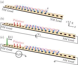
Figure 1: Schematic view of two-terminal setups where FM wire, modeled as 1D chain of ferromagnetic atoms Spinelli2014 , hosts SW comprised of $N=10$ localized magnetic moments $\mathbf{M}_{i}(t)$ precessing as classical vectors with frequency $\omega$ and cone angle $\theta=10^{\circ}$ Demidov2007 , as well as with harmonic variation in the phase of precession of adjacent moments. The wire is attached to L and R semi-infinite NM leads which terminate into the macroscopic reservoirs where in: (a) no bias voltage is applied between the reservoirs; (b) small bias voltage $V_{b}$ is applied to inject dc unpolarized charge current into the wire, which is then spin-polarized by three fixed spins (red arrows); and (c) Lorentzian voltage pulse Ivanov1997 ; Keeling2006 is applied between the reservoirs to inject leviton current pulse $I_{\mathrm{L}}(t)$ into the wire carrying charge $\int\!\!dt\,I_{\mathrm{L}}(t)=2e$.

The nonequilibrium many-body perturbation theory Mahfouzi2014 ; Zheng2017 , formulated using Feynman diagrams for nonequilibrium Green function (GF) Stefanucci2013 , offers rigorous quantum-mechanical treatment of both electrons and magnons, once the original spin operators are mapped to the bosonic ones Kiselev2000 . However, to ensure current conservation, one has to sum large classes of such diagrams Mera2016 which can lead to errors due to missed vertex corrections Gukelberger2015 . Furthermore, due to small magnon bandwidth, small electron-magnon interaction constant $J_{sd}$ in the realm of electrons can become strongly correlated regime for magnons due to large ratio $J_{sd}/$magnon-bandwidth. This can lead to quasibound states of magnons surrounded by electron-hole pairs Mahfouzi2014 , therefore suggesting that complicated higher order diagrams should be evaluated. This severely limits system size in two-terminal geometries of Fig. 1 or time scale over which electronic spin and charge currents, or magnonic spin current, can be computed. Since both electrons and magnons have intrinsic angular momentum, their translational flow leads to a flux of spin angular momentum as spin current.

On the other hand, experiments Zilberman1995 ; Woo2017 ; Demidov2007 ; Evelt2017 exciting dipole or exchange dominated SWs are commonly interpreted using classical micromagnetics Kim2010 or atomistic spin dynamics Evans2014 simulations (the latter is akin to the former but with atomistic discretization). They describe SWs using trajectories of classical vectors $\mathbf{M}_{i}(t)$ of fixed (unit) length, pointing along the direction of localized magnetic moments, which precesses around an easy axis with frequency $\omega$ and precession cone angle $\theta$, as illustrated in Fig. 1. The cone angle has been measured Demidov2007 as $\theta\lesssim 10^{\circ}$.

In this study, we employ recently developed multiscale and nonperturbative (i.e., numerically exact) time-dependent-quantum-transport/classical-atomistic-spin-dynamics formalism Petrovic2018 ; Bajpai2019a ; Petrovic2019 to the problem of electron-SW interaction. This makes possible treating large number of time-dependent localized spins in experimentally relevant noncollinear configurations and over technologically relevant time scales $\sim 1$ ns. The formalism combines time-dependent nonequilibrium Green function (TDNEGF) Stefanucci2013 ; Gaury2014 description of electrons out of equilibrium in open quantum systems, such as those illustrated in Fig. 1, with the Landau-Lifshitz-Gilbert (LLG) equation describing classical dynamics of localized magnetic moments. The classical treatment of localized magnetic moments is justified Wieser2015 in the limit of large localized spins $S\rightarrow\infty$ and $\hbar\rightarrow 0$ (while $S\times\hbar\rightarrow 1$), as well as in the absence of entanglement Mondal2019 between quantum state of localized spins which is expected to be satisfied at room temperature.

The paper is organized as follows. In Sec. II we introduce SW solution and its coupling to quantum Hamiltonian of electrons and TDNEGF calculations. Since explanation of electron-SW scattering for dc injected electronic current [Sec. III.3] or leviton current pulse [Sec. III.4] crucially relies on understanding of how SW pumps spin and charge currents in the absence of any bias voltage, we carefully analyze the origin of such pumping in Sec. III.1 and Sec. III.2, respectively. This includes computation of nonadiabaticity angle between nonequilibrium electronic spin density and localized magnetic moments in Sec. III.2 which visualizes time-retardation effects. We conclude in Sec. IV.

II Models and Methods

Since we assume that a single coherent SW has been excited externally, such as by microwave current flowing through narrow antennas Evelt2017 , we fix dynamics of localized magnetic moment $\mathbf{M}_{i}(t)$ at site $i$ of a one-dimensional (1D) lattice to be the SW solution Kim2010 ; Evans2014 of the LLG equation (for simplicity without damping):

$$\mathrm{M}_{i}^{x}(t) = \sin\theta\ \mathrm{cos}\left(kx_{i}+\omega t\right),$$ (1a)

$$\mathrm{M}_{i}^{y}(t) = \sin\theta\ \mathrm{sin}\left(kx_{i}+\omega t\right),$$ (1b)

$$\mathrm{M}_{i}^{z}(t) = \cos\theta.$$ (1c)

Due to 1D geometry, the wavevector is just a number $k=2\pi/[a(N-1)]=2\pi/\lambda$, while the discrete coordinate is $x_{i}=(i-1)a$ and $N$ is the total number of localized magnetic moments. Note that the uniform mode–which describes all magnetic moments precessing in-phase in magnetic materials driven by microwaves under the ferromagnetic resonance conditions Tserkovnyak2005 —is obtained by setting $k=0$. Even though we employ 1D geometry as a toy model of a realistic three-dimensional FM layer, such 1D geometries can be realized experimentally, such as by using an artificial chain of ferromagnetically coupled Fe atoms whose SWs are excited and detected using atom-resolved inelastic tunneling spectroscopy in a scanning tunneling microscope Spinelli2014 . We note that solution in Eq. (1) also appears in classical micromagnetics Kim2010 , but there $\mathbf{M}_{i}$ represents magnetization of a small volume of space, typically (2–10 nm)³, rather than of individual atoms Evans2014 that we must assume in order to couple classical dynamics of $\mathbf{M}_{i}(t)$ to time-dependent quantum transport calculations where electrons hop from atom to atom.

The FM nanowire hosting such SW is an active region of devices in Fig. 1, which is attached to two normal metal (NM) semi-infinite leads terminating into the macroscopic reservoirs. We use three different two-terminal geometries depicted Fig. 1: (a) no bias voltage $V_{b}$ is applied between the left (L) and right (R) reservoirs kept at the same chemical potential $\mu_{\mathrm{L}}=\mu_{\mathrm{R}}$; (b) small dc bias voltage, $eV_{b}=\mu_{\mathrm{L}}-\mu_{\mathrm{R}}=0.01$ eV, is applied between the reservoirs to inject unpolarized charge current into the active region where electrons are spin-polarized by three static localized magnetic moments [red arrows in Fig. 1(b)] pointing along the $z$-axis; and (c) the Lorentzian voltage pulse Ivanov1997 ; Keeling2006 applied to the left NM lead injects a leviton current pulse $I_{\mathrm{L}}(t)$ carrying charge $\int\!\!dt\,I_{\mathrm{L}}(t)=2e$, which is then spin-polarized by the same three static localized magnetic moments as in (b).

The quantum Hamiltonian of electrons within the FM nanowire is chosen as 1D tight-binding model

$$\hat{H}(t)=-\sum_{\braket{ij}}\gamma_{ij}\hat{c}_{i}^{\dagger}\hat{c}_{j}-J_{sd}\sum_{i}\hat{c}_{i}^{\dagger}{\bm{\sigma}}\cdot\mathbf{M}_{i}(t)\hat{c}_{i},$$ (2)

with an additional $sd$ exchange interaction of strength $J_{sd}=0.5$ eV Cooper1967 between the spins of the conduction electrons, described by the vector of the Pauli matrices ${\bm{\sigma}}=(\hat{\sigma}_{x},\hat{\sigma}_{y},\hat{\sigma}_{z})$, and $\mathbf{M}_{i}(t)$ from Eq. (1). Here $\hat{c}_{i}^{\dagger}=(\hat{c}_{i\uparrow}^{\dagger}\ \ \hat{c}_{i\downarrow}^{\dagger})$ is a row vector containing operators $\hat{c}_{i\sigma}^{\dagger}$ which create an electron with spin $\sigma=\uparrow,\downarrow$ at site $i$; $\hat{c}_{i}$ is a column vector containing the corresponding annihilation operators; and $\gamma_{ij}=1$ eV is the nearest-neighbor hopping. The NM leads are described by the same Hamiltonian as in Eq. (2) but with $J_{sd}\equiv 0$.

The fundamental quantity of nonequilibrium quantum statistical mechanics is the density matrix. The time-dependent one-particle density matrix can be expressed Gaury2014 , ${\bm{\rho}_{\rm neq}}(t)=\mathbf{G}^{<}(t,t)/i$, in terms of the lesser GF of TDNEGF formalism defined by $G^{<,\sigma\sigma^{\prime}}_{ii^{\prime}}(t,t^{\prime})=i\langle\hat{c}^{\dagger}_{i^{\prime}\sigma^{\prime}}(t^{\prime})\hat{c}_{i\sigma}(t)\rangle$ where $\langle\ldots\rangle$ is the nonequilibrium statistical average Stefanucci2013 . We solve a matrix integro-differential equation Popescu2016

$$i\hbar\frac{d{\bm{\rho}}_{\rm neq}}{dt}=[\mathbf{H}(t),{\bm{\rho}}_{\rm neq}]+i\sum_{p=L,R}[{\bm{\Pi}}_{p}(t)+{\bm{\Pi}}_{p}^{\dagger}(t)],$$ (3)

for the time evolution of ${\bm{\rho}_{\rm neq}}(t)$ where $\mathbf{H}(t)$ is the matrix representation of Hamiltonian in Eq. (2). This can be viewed as an exact master equation for the reduced density matrix of an open finite-size quantum system attached to macroscopic Fermi liquid reservoirs via semi-infinite NM leads. The leads ensure continuous energy spectrum of the system and, thereby, dissipation. The ${\bm{\Pi}}_{p}(t)$ matrices

$${\bm{\Pi}}_{p}(t)=\int_{t_{0}}^{t}\!\!dt_{2}\,[\mathbf{G}^{>}(t,t_{2}){\bm{\Sigma}}_{p}^{<}(t_{2},t)-\mathbf{G}^{<}(t,t_{2}){\bm{\Sigma}}_{p}^{>}(t_{2},t)],$$ (4)

are expressed in terms of the lesser and greater GF and the corresponding self-energies ${\bm{\Sigma}}_{p}^{>,<}(t,t^{\prime})$ Popescu2016 . They yield directly time-dependent total charge, $I_{p}(t)=\frac{e}{\hbar}\mathrm{Tr}\,[{\bm{\Pi}}_{p}(t)]$, and spin, $I_{p}^{S_{\alpha}}(t)=\frac{e}{\hbar}\mathrm{Tr}\,[\hat{\sigma}_{\alpha}{\bm{\Pi}}_{p}(t)]$, currents flowing into the lead $p=\mathrm{L},\mathrm{R}$. Local currents Bajpai2019 , or any other local quantity within the active region, are obtained by tracing the corresponding operator with ${\bm{\rho}_{\rm neq}}(t)$. We use the same units for charge and spin currents, defined as $I_{p}=I_{p}^{\uparrow}+I_{p}^{\downarrow}$ and $I_{p}^{S_{\alpha}}=I_{p}^{\uparrow}-I_{p}^{\downarrow}$, in terms of spin-resolved charge currents $I_{p}^{\sigma}$. In our convention, positive current in NM lead $p$ means charge or spin is flowing out of that lead.

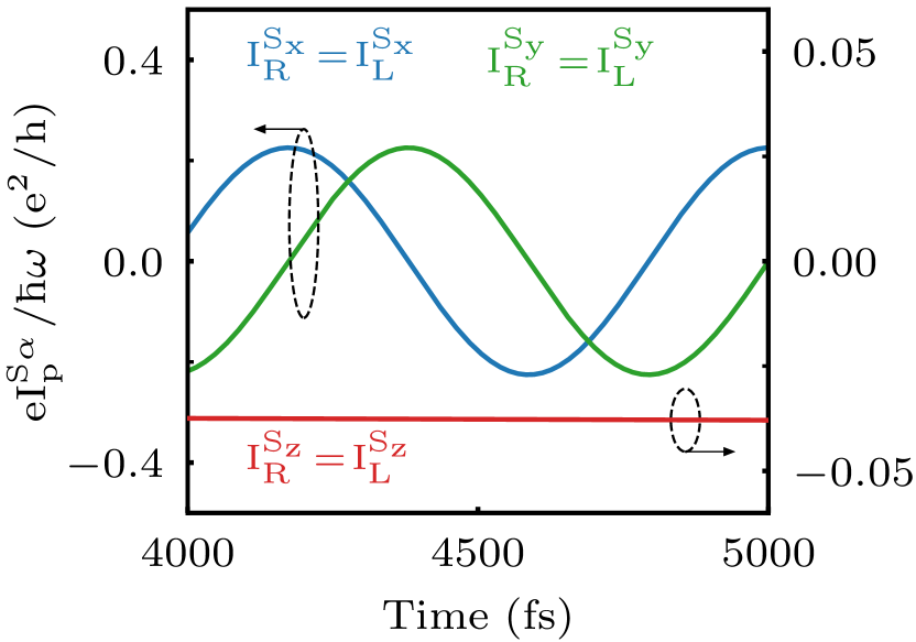
Figure 2: Time-dependence of electronic spin currents $I_{\mathrm{L}}^{S_{\alpha}}(t)=I_{\mathrm{R}}^{S_{\alpha}}(t)$ pumped symmetrically Tserkovnyak2005 ; Chen2009 into the L and R NM leads of setup in Fig. 1(a) whose localized magnetic moments precess as a uniform mode with $k=0$ in Eq. (1). The Fermi energy is chosen as $E_{F}=-1.6$ eV, the frequency of precession is $\hbar\omega=0.005$ eV, the total number of localized magnetic moments is $N=10$ and dc bias voltage is absent $V_{b}\equiv 0$.

III Results

III.1 Spin-wave-driven chiral spin pumping

As a warm-up, we first consider standard Tserkovnyak2005 ; Chen2009 ; Mahfouzi2012 ; Dolui2019 spin pumping by the uniform mode, with $k=0$ in Eq. (1) and no dc bias voltage applied, which will serve as a reference point for subsequent discussion. In this case, identical pure (i.e., not accompanied by any charge current) spin currents $I_{\mathrm{L}}^{S_{\alpha}}(t)=I_{\mathrm{R}}^{S_{\alpha}}(t)$ are pumped into both leads, as shown in Fig. 2. Their $I_{\mathrm{L}}^{S_{z}}=I_{\mathrm{R}}^{S_{z}}$ components are time independent, and their negative sign shows that they flow into the NM leads, as obtained also in the scattering theory Tserkovnyak2005 , rotating frame approach Chen2009 or Floquet-NEGF theory Mahfouzi2012 ; Dolui2019 .

On the other hand, the excited SW in the setup of Fig. 1(a) pumps both charge and spin currents into the NM leads in the absence of any dc bias voltage. Their time dependences, $I_{p}^{S_{\alpha}}(t)$ and $I_{p}(t)$, are shown in Fig. 2 after transient currents have died out. Furthermore, in contrast to pumping by the uniform mode, we find $|I_{\mathrm{L}}^{S_{z}}|>|I_{\mathrm{R}}^{S_{z}}|$. This is due to the spin current carried by the SW itself Sandweg2011 . That is, spin current carried by the SW must be “transmuted” Bauer2011 into electronic spin current at the FM-wire/NM-left-lead interface Sandweg2011 ; Woo2017 ; Petrovic2019 because no localized magnetic moments exist in the NM lead to support transport of angular momentum via their dynamics. This current is then added or subtracted to symmetrically pumped spin currents into the left or right NM leads, respectively. This interpretation is supported by the fact that changing the sign of $k$ in Eq. (1) leads to a reversed situation, $|I_{\mathrm{L}}^{S_{z}}|<|I_{\mathrm{R}}^{S_{z}}|$.

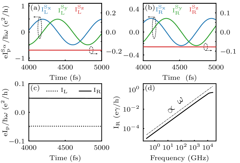
Figure 3: Time-dependence of electronic spin currents pumped into the (a) left and (b) right NM leads of setup in Fig. 1(a) whose localized magnetic moments precess as coherent SW mode with $k\neq 0$ in Eq. (1). (c) The SW with its nonuniform precessing magnetic moments also pumps dc charge current $I_{\mathrm{L}}=-I_{\mathrm{R}}$ into the NM leads, whose dependence on frequency (solid line) in panel (d) is linear $\propto\omega$ (dash-dot line). The Fermi energy is chosen as $E_{F}=-1.6$ eV, the frequency of SW is $\hbar\omega=0.005$ eV, the total number of localized magnetic moments is $N=10$ and dc bias voltage is absent, $V_{b}\equiv 0$.

III.2 Spin-wave-driven chiral charge pumping

The charge pumping in spintronic devices with excited coherent SWs was observed experimentally in compressively strained (Ga,Mn)As bar Ciccarelli2014 , as well as in YIG/graphene Evelt2017 . In the latter case, SW is excited within insulating YIG while pumped current flows through metallic graphene where localized magnetic moments are induced by proximity exchange coupling Hallal2017 . However, both of these experimental setups require SOC, unlike our setup in Fig. 1(a) where SOC is absent.

In the adiabatic limit Stahl2017 , the conduction electron spin at site $i$, $\langle\hat{\mathbf{s}}_{i}\rangle_{t}=\frac{\hbar}{2}\mathrm{Tr}\,[{\bm{\rho}}_{\mathrm{neq}}(t)|i\rangle\langle i|\otimes{\bm{\sigma}}]$, follows strictly the direction of localized magnetic moment $\mathbf{M}_{i}(t)$ at the same site. In this limit, the charge pumping by time-dependent noncoplanar and noncollinear magnetic texture, described by local magnetization $\mathbf{m}(\mathbf{r},t)$ as a continuous variable, is predicted by the spin motive force (SMF) theory Volovik1987 ; Barnes2007 ; Duine2008 ; Tserkovnyak2008a ; Zhang2009b

$$j_{\alpha}(\mathbf{r})=C[\partial_{\alpha}\mathbf{m}(\mathbf{r},t)\times\mathbf{m}(\mathbf{r},t)]\cdot\partial_{t}\mathbf{m}(\mathbf{r},t).$$ (5)

This formula is rooted in the associated geometrical Berry phase. Here ${\bm{\rho}}_{\mathrm{eq}}$ is the equilibrium density matrix; $C=PG_{0}\hbar/2e$; $P=(G^{\uparrow}-G^{\downarrow})/(G^{\uparrow}+G^{\downarrow})$ is the spin polarization of the ferromagnet; and $G_{0}=G^{\uparrow}+G^{\downarrow}$ is the total conductivity. We use notation $\partial_{t}=\partial/\partial t$ and $\partial_{\alpha}=\partial/\partial\alpha$ for $\alpha\in\{x,y,z\}$. If we plug SW solution for the local magnetization—$m_{x}(x)=\sin\theta\cos(kx+\omega t)$; $m_{y}(x)=\sin\theta\sin(kx+\omega t)$; and $m_{z}(x)=\cos\theta$—into Eq. (5) we obtain zero pumped charge current, $j_{x}(x)\equiv 0$.

It is worth clarifying that if plug SW solution from Eq. (1) into the discretized version of Eq. (5)

$$j_{x}(i)=\frac{C}{a}\left[\partial_{t}\mathbf{M}_{i}\times\mathbf{M}_{i+1}\right]\cdot\mathbf{M}_{i},$$ (6)

we actually obtain a nonzero result, $j_{x}(i)=\frac{C\omega}{a}\sin\theta\sin 2\theta\sin^{2}(ka/2)$. This apparently contradicts $j_{x}(x)\equiv 0$ obtain from the continuous formula in Eq. (5). However, in the limit of the lattice spacing going to zero, $a\rightarrow 0$, we have $\lim_{a\to 0}\frac{1}{a}\sin^{2}(ka/2)=0$ and, therefore, the same conclusion, $j_{x}(i)\equiv 0$.

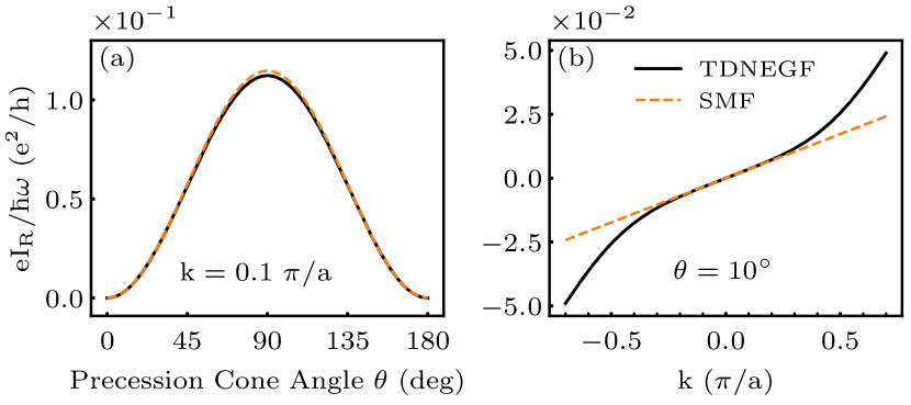
Figure 4: The dependence of charge current from Fig. 3(c) on: (a) precession cone angle $\theta$; and (b) wavevector $k$ of the SW. The solid lines are obtained from TDNEGF calculations and the dashed line is obtained from modified Evelt2017 SMF formula in Eq. (8).

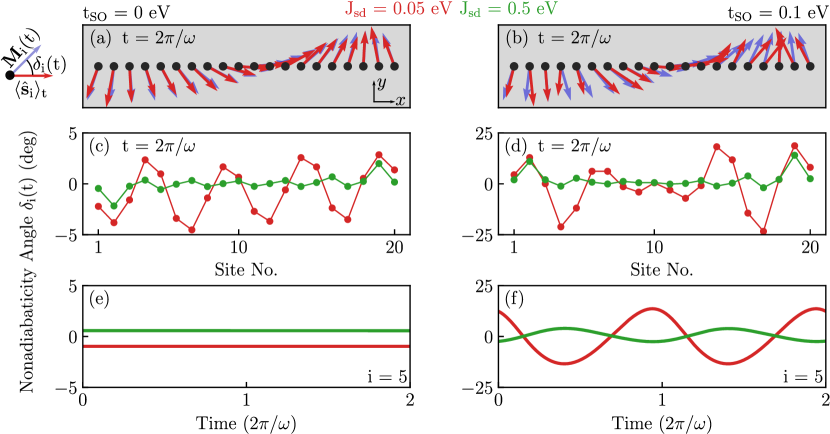
Figure 5: (a),(b) Spatial profile at time $t=2\pi/\omega$ of the in-$xy$-plane component of nonequilibrium electronic spin density vector $\langle\hat{\mathbf{s}}_{i}\rangle_{t}$ and localized magnetic moments $\mathbf{M}_{i}(t)$ across FM nanowire hosting a SW of wavevector $k\simeq 0.2a$. Inset on the left illustrates the nonadiabaticity angle $\delta_{i}$ between these two vectors. (c),(d) Spatial profile of nonadiabaticity angle $\delta_{i}(t)$ at time $t=2\pi/\omega$. (e),(f) Time dependence of $\delta_{i=5}(t)$ at site $i=5$. In panels (a),(c),(e) SOC is absent, while in panels (b),(d),(f) we use Rashba SOC in Eq. (9) of strength $t_{\mathrm{SO}}=0.1$ eV. Two different values of $sd$ exchange interaction in the Hamiltonian [Eq. (2)] are used, $J_{sd}=0.05$ eV (red lines) and $J_{sd}=0.5$ eV (green lines). The Fermi energy is chosen as $E_{F}=-1.6$ eV, the frequency of SW is $\hbar\omega=0.005$ eV, the total number of localized magnetic moments is $N=20$ and dc bias voltage is absent, $V_{b}\equiv 0$.

In Ref. Evelt2017 , a modified version of the SMF formula

$$j_{\alpha}(\mathbf{r})=C[\partial_{\alpha}\mathbf{m}(\mathbf{r},t)\times\mathbf{m}(\mathbf{r},t)+\beta\partial_{\alpha}\mathbf{m}(\mathbf{r},t)]\cdot\partial_{t}\mathbf{m}(\mathbf{r},t),$$ (7)

was employed to explain the experiment. Here adding nonadiabatic correction of magnitude $\beta$ to purely geometrical first term was justified Evelt2017 as the consequence of slight misalignment between electron spin and localized magnetic moments caused by SOC and thereby induced relaxation of nonequilibrium electron spin density. Thus, using SW solution in the discretized version of $\beta$-term in Eq. (7) gives

$$j_{x}^{\beta}(i) = C\beta\partial_{t}\mathbf{M}_{i}\cdot\left(\frac{\mathbf{M}_{i+1}-\mathbf{M}_{i}}{a}\right)$$ (8)

$$= C\beta\omega\sin^{2}\theta\,\left(\frac{\sin ka}{a}\right)\xrightarrow[a\to 0]{}Ck\omega\sin^{2}\theta.$$

The final result explains experimentally observed Evelt2017 chiral nature of pumping where charge current changes sign upon $k\rightarrow-k$.

We compare this result with the one from TDNEGF calculations in Fig. 4, where they track each other [Fig. 4(a)] as a function of cone angle $\theta$, except around $\theta=90^{\circ}$; as well as as a function of $k$ [Fig. 4(a)] within $|k|\lesssim 0.2\pi/a$ interval. Since our TDNEGF calculations are numerically exact, such deviations (for values of $\theta$ and $k$ not commonly found in experiments though Woo2017 ; Demidov2007 ) stem from the fact that the SMF formula in Eq. (7) contains only the lowest order Duine2008 time and spatial derivatives of local magnetization.

This also demonstrates how TDNEGF calculations automatically include nonadiabatic effects in spin dynamics even when SOC is zero. The origin of $\beta$-term in Eq. (7) in the absence of SOC, which is effectively generated by TDNEGF calculations in Fig. 4, is that direction of nonequilibrium electron spin density at site $i$, $\langle\hat{\mathbf{s}}_{i}\rangle_{t}$, is always somewhat behind the ‘adiabatic direction’ set by the classical vector $\mathbf{M}_{i}(t)$. So, the nonadiabaticity results from the fact that the motion of the classical spin affects the conduction electrons in a retarded way Sayad2015 —it takes a finite time until the local conduction electron spin $\langle\hat{\mathbf{s}}_{i}\rangle_{t}$ reacts to the motion of the classical spin. This is visualized in Fig. 5(a),(c) where nonadiabaticity angle $\delta_{i}(t)$ between $\langle\hat{\mathbf{s}}_{i}\rangle_{t}$ and $\mathbf{M}_{i}(t)$ decreases with increasing $J_{sd}$ (realistic values measured experimentally are $J_{sd}\simeq 0.1$ eV Cooper1967 ). In the absence of SOC, the angle $\delta_{i}(t)$ in Fig. 5(e) is time independent. The resulting spin torque, $\propto\langle\hat{\mathbf{s}}_{i}\rangle_{t}\times\mathbf{M}_{i}(t)$, exerted on the classical localized magnetic moment acts then like an additional Gilbert damping which is, generally, described by nonlocal-in-time damping kernel with memory effects Bajpai2019a ; Sayad2015 ; Hurst2020 . Note, however, that we fix the dynamics of localized magnetic moments to SW solutions in Eq. (1), rather than solving TDNEGF and LLG equations self-consistently Petrovic2018 ; Bajpai2019a ; Petrovic2019 .

For comparison, in Fig. 5(b),(d) we use additional Rashba SOC term Manchon2015 in the quantum Hamiltonian in Eq. (2)

$$\hat{H}_{\mathrm{SO}}=\sum_{ij}\hat{c}_{i}^{\dagger}\mathbf{t}_{ij}\hat{c}_{j},$$ (9)

where $\mathbf{t}_{ij}=-it_{\mathrm{SO}}\hat{\sigma}_{y}$ for $i=j+1$. The strength of the Rashba SOC is chosen as $t_{\mathrm{SO}}=0.1$ eV, which generates conventional static Gilbert damping $\alpha_{\mathrm{G}}=0.01$ via the scattering theory Brataas2011 as the typical value Taniguchi2015 found in FM nanowires. This additional Rashba SOC leads to increase of $\delta_{i}$ in Fig. 5(b),(d) when compared to Fig. 5(a),(c), respectively. It also generates periodic time dependence of $\delta_{i}(t)$ in Fig. 5(f).

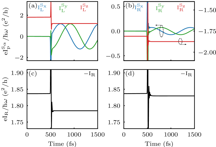
Figure 6: Time-dependence of electronic spin currents in the (a) left and (b) right NM leads of setup in Fig. 1(b) whose localized magnetic moments start to precess at $t=500$ fs as a coherent SW with $k\neq 0$ in Eq. (1) in the presence of a flux of electrons injected into the active region by dc bias voltage $eV_{b}=0.01$ eV. The electrons are spin-polarized by three fixed spins (red arrows) in Fig. 1(b). The corresponding time-dependence of their charge current $I_{\mathrm{R}}(t)$ is shown in panel (c). Panel (d) plots time dependence of $I_{\mathrm{R}}(t)$ for “frozen-in-time” Starikov2018 SW where $t=0$ in Eq. (1). The Fermi energy is chosen as $E_{F}=-1.6$ eV, the frequency of SW is $\hbar\omega=0.005$ eV, the total number of localized magnetic moments is $N=10$ and dc bias voltage is $V_{b}=0.01$ V.

Another way to interpret the origin of charge pumping by SW is to analyze its frequency dependence shown in Fig. 3(d). This complies with the general theory of “adiabatic” quantum pumping Moskalets2002 ; FoaTorres2005 ; Bajpai2019 since it scales linearly with frequency in the physically relevant frequency range GHz–THz Jungfleisch2018 . Note that terminology “adiabatic” in this context is not related to spin (unlike the preceding discussion where adiabatic means that flowing electron spin and localized spins are aligned instantaneously Stahl2017 )—instead it signifies sufficiently slow change of harmonic potential driving the quantum system so that its frequency is $\hbar\omega\ll E_{F}$ and/or smaller than relevant relaxation time for electrons. In contrast, charge pumping by SW in YIG/graphene heterostructure with SOC peaks between 5 and 7 GHz Evelt2017 . We recall that such linear scaling is in accord with the key requirement—breaking of left-right symmetry—for nonzero dc component of quantum charge pumping by a time-dependent potential Moskalets2002 ; FoaTorres2005 ; Bajpai2019 . This can be achieved by breaking inversion symmetry and/or time-reversal symmetry. In the “adiabatic” regime, quantum charge pumping requires both inversion and time-reversal symmetries to be broken dynamically, such as by two spatially separated potentials oscillating out-of-phase Moskalets2002 , which leads to $\bar{I}_{p}(t)\propto\omega$ at low frequencies ($\bar{A}$ is the average of quantity $A$ over one period). In the case of SW, it is the wave-like pattern of precessing localized magnetic moments which dynamically breaks the left-right symmetry in Fig. 1(a), with respect to vertical plane positioned between moments localized at sites $i=N/2$ and $i=N/2+1$. In contrast, in the “nonadiabatic” regime only one of those two symmetries needs to be broken and this does not have to occur dynamically. The dc component of the pumped current in the “nonadiabatic“ regime is FoaTorres2005 $\bar{I}_{p}(t)\propto\omega^{2}$ at low frequencies as obtained in, e.g., the case of charge pumping by uniform mode across potential barrier that breaks the left-right symmetry of the device statically Chen2009 .

Figure 7: Time-dependence of electronic spin currents $I_{\mathrm{R}}^{S_{\alpha}}(t)$ in the right NM lead after unpolarized leviton is injected by the Lorentzian voltage pulse Ivanov1997 ; Keeling2006 into the active region hosting: (a) three static localized magnetic moments (red arrows) pointing along the $z$-axis, acting as spin-polarizer, followed by SW excited at $t=500$ fs, as illustrated in Fig. 1(c); (b) three static localized magnetic moments and a “frozen-in-time” SW excited at $t=500$ fs. Panels (c) and (d) show time dependence of the charge current $I_{\mathrm{R}}(t)$ corresponding to (a) and (b), respectively. In addition, panels (b) and (d) plot (dotted lines) time dependence of $I_{\mathrm{R}}^{S_{\alpha}}(t)$ and $I_{\mathrm{R}}(t)$, respectively, for the active region containing only the three static localized magnetic moments pointing along the $z$-axis. The Fermi energy is chosen as $E_{F}=-1.6$ eV, the frequency of SW is $\hbar\omega=0.005$ eV and the total number of localized magnetic moments is $N=10$.

III.3 Electron/spin-wave scattering for injected dc spin-polarized charge current

For the setup in Fig. 1(b), we first establish (after some transient period not shown explicitly) steady charge current $I_{\mathrm{R}}$ [flat line in Fig. 6(c) for $t<500$ fs] of electrons injected by dc bias voltage into $3+10$ static localized magnetic moments oriented along the $z$-axis. The initially unpolarized current becomes spin-polarized due to static moments, as characterized by steady spin current $I_{\mathrm{R}}^{S_{z}}\neq 0$ [flat line in Fig. 6(b) for $t<500$ fs] and the corresponding spin-polarization $P_{z}=|I_{\mathrm{R}}^{S_{z}}|/|I_{\mathrm{R}}|\approx 50$%. Then at $t=500$ fs we suddenly excite SW composed of $10$ precessing localized magnetic moments in Fig. 1(b). This induces transient currents around that instant which help us to visualize the boundary between the time interval without and with SW being present. Within the time interval $t>500$ fs where SW is present, new time-dependent spin currents $I_{p}^{S_{x}}(t)$ and $I_{p}^{S_{y}}(t)$ emerge [Fig. 6(a),(b)] due to spin pumping by SW demonstrated in Fig. 3(a),(b).

Concurrently, dc spin currents $I_{\mathrm{L}}^{S_{z}}$ [Fig. 6(a)] and $I_{\mathrm{R}}^{S_{z}}$ [Fig. 6(b)], as well as dc charge current $I_{\mathrm{R}}$ [Fig. 6(c)], are reduced compared to their values prior to SW excitation. This reduction is mostly due to charge and spin currents pumped in the direction right-NM-lead$\rightarrow$left-NM-lead in Fig. 3, which is opposite to the flow of originally injected charge and spin currents by dc bias voltage. Thus, outflowing spin and charge currents in the right NM lead can also be enhanced if we invert the sign of $k$ in Eq. (1) and, therefore, the direction of SW propagation. Another reason for the reduction is backscattering of electrons by time-dependent potential generated by SW, whose magnitude for charge current shown in Fig. 6(c) we estimate using $[I_{\mathrm{R}}(t<500\ \mathrm{fs})-I_{\mathrm{R}}(t>500\ \mathrm{fs})+I_{\mathrm{R}}^{\mathrm{SW}}]/I_{\mathrm{R}}(t<500\ \mathrm{fs})$ to be less than $1$%. Here $I_{\mathrm{R}}^{\mathrm{SW}}$ denotes charge current pumped by SW [Fig. 3(c)] in the absence of dc bias voltage.

Recent time-independent quantum transport calculations Starikov2018 of the resistance of FM have include “frozen magnons” as correlated spin disorder where localized spins are tilted away from the easy axis in accord with thermal population of magnon modes. To understand time-dependent effects missed in such calculations, we freeze localized magnetic moments by setting $t=0$ in Eq. (1). The scattering from such “frozen-in-time” SW leads to much smaller current reduction in Fig. 6(d).

III.4 Electron/spin-wave scattering for injected spin-polarized charge current leviton pulse

In order to simulate single-electron/single-SW scattering, we inject pulsed current into the active region using the Lorentzian voltage pulse Popescu2016 , $V_{\mathrm{L}}(t)=2\hbar\tau/[(t-t_{0})^{2}+\tau^{2}]$, where the pulse duration is $\tau=7.5\hbar/\gamma$. As confirmed experimentally Dubois2013 , such special pulse profile with $\frac{e}{\hbar}\int\!\!dt\,V_{\mathrm{L}}(t)=2\pi n$ Moskalets2016 drives the Fermi sea in the left reservoir to ensure Ivanov1997 ; Keeling2006 excitation of an integer number $n$ of purely electronic states above the sea. They appear without spurious electron-hole pairs and exhibit minimal Gaury2016 nonequilibrium noise in charge transfer across the active region. We use $n=2$, so that injected unpolarized charge current pulse, called leviton Dubois2013 , carries charge $\int\!\!dt\,I_{\mathrm{L}}(t)=2e$. This can be viewed as minimalistic unpolarized current composed of one spin-$\uparrow$ and one spin-$\downarrow$ electron flowing together. Upon spin-polarization by three static localized magnetic moments in Fig. 1(c), the leviton interacts with SW excited suddenly at $t=500$ fs. After such interaction, leviton outflows into the right NM lead where its spin and charge currents are plotted in Figs. 7(a) and  7(c), respectively. For comparison, Figs. 7(b) and  7(d) plot spin and charge currents in the right NM lead, respectively, for a leviton interacting with “frozen-in-time” SW. In addition, Figs. 7(b) and  7(d) also include (dotted lines) spin and charge current of leviton outflowing into the right NM lead when SW in Fig. 1(c) is removed from the active region. The integrals for outflowing spin-polarized leviton after scattering from SW in Figs. 7(a) and  7(c) are $\int\!\!dt\,I_{\mathrm{R}}^{S_{z}}(t)=0.939e$ and $\int\!\!dt\,I_{\mathrm{R}}(t)=0.822e$, respectively. They can be compared to $\int\!\!dt\,I_{\mathrm{R}}^{S_{z}}(t)=0.944e$ and $\int\!\!dt\,I_{\mathrm{R}}(t)=0.827e$ in Figs. 7(b) and  7(d), respectively. Note that the the ratio of integrals of two dotted curves in Figs. 7(b) and  7(d) is $P_{z}=|\int\!\!dt\,I_{\mathrm{R}}^{S_{z}}(t)|/|\int\!\!dt\,I_{\mathrm{R}}(t)|\approx 40$% which can be considered as the spin-polarization of leviton after passing through three static localized magnetic moments in Fig. 1(c).

IV Conclusions

In conclusion, using time-dependent-quantum-transport/classical-atomistic-spin-dynamics multiscale framework Petrovic2018 ; Bajpai2019a ; Petrovic2019 we predict that SW coherently excited within a metallic ferromagnet will pump chiral electronic charge and spin currents into the attached normal metal leads. The chirality of pumped currents means that their direction is tied to the direction of SW propagation, changing upon reversal of the SW wavevector. The pumped currents scale linearly with the frequency of the SW in experimentally relevant GHz–THz range. In contrast, recent experiments on “magnonic charge pumping” Ciccarelli2014 ; Evelt2017 were interpreted by requiring nonzero SOC to introduce misalignment between electron spin and localized magnetic moments, thereby adding nonadiabatic contribution Evelt2017 to the spin motive force formula Volovik1987 ; Barnes2007 ; Duine2008 ; Tserkovnyak2008a ; Zhang2009b . This formula describes charge pumping by time-dependent noncoplanar and noncollinear magnetic textures. Although SW is an example of such texture, standard purely adiabatic (i.e., for electron spin and localized spins aligned instantaneously) spin motive force formula [Eq. (5)] valid in the absence of SOC predicts zero pumped charge current [Sec. III.2]. Thus our prediction reveals the importance of time-retardation effects Bajpai2019a ; Sayad2015 , where conduction electron spin is always somewhat behind the ‘adiabatic direction’ set by the classical localized spins. The retardation is visualized [Fig. 5] by plotting the nonadiabaticity angle between conduction electron spin and classical localized magnetic moment, both in the absence and presence of SOC. When dc spin-polarized charge current is injected into the ferromagnet, electrons interact with SW in such a way that the outflowing charge and spin current are changed both by the scattering off time-dependent potential generated by the SW and superposition with the currents pumped by the SW itself. Using Lorentzian voltage pulse to excite leviton out of the Fermi sea, which carries one electron charge with no accompanying electron-hole pairs and behaves as soliton-like quasiparticle, we also show how a single electron scatters from a single SW.

- (1) S.-K. Kim, Micromagnetic computer simulations of spin waves in nanometre-scale patterned magnetic elements, J. Phys. D: Appl. Phys. 43, 264004 (2010).
- (2) R. F. L. Evans, W. J. Fan, P. Chureemart, T. A. Ostler, M. O. A. Ellis, and R. W. Chantrell, Atomistic spin model simulations of magnetic nanomaterials, J. Phys.: Condens. Matter 26, 103202 (2014).
- (3) B. Jungfleisch, W. Zhang, and A. Hoffmann, Perspectives of antiferromagnetic spintronics, Phys. Lett. A 382, 865 (2018).
- (4) C. P. Hofmann, Spontaneous magnetization of an ideal ferromagnet: Beyond Dyson’s analysis, Phys. Rev. B 84, 064414 (2011).
- (5) P. E. Zil’berman, A. G. Terniryazev, and M. P. Tikhornirova, Excitation and propagation of exchange spin waves in films of yttrium iron garnet, JETP 81, 151 (1995).
- (6) V. E. Demidov, U.-H. Hansen, and S. O. Demokritov, Spin-wave eigenmodes of a saturated magnetic square at different precession angles, Phys. Rev. Lett. 98, 157203 (2007).
- (7) M. Evelt, H. Ochoa, O. Dzyapko, V. E. Demidov, A. Yurgens, J. Sun, Y. Tserkovnyak, V. Bessonov, A. B. Rinkevich, and S. O. Demokritov, Chiral charge pumping in graphene deposited on a magnetic insulator, Phys. Rev. B 95, 024408 (2017).
- (8) S. Woo, T. Delaney, and G. S. D. Beach, Magnetic domain wall depinning assisted by spin wave bursts, Nat. Phys. 13, 448 (2017).
- (9) C. Tzschaschel, K. Otani, R. Iida, T. Shimura, H. Ueda, S. Günther, M. Fiebig, and T. Satoh, Ultrafast optical excitation of coherent magnons in antiferromagnetic NiO, Phys. Rev. B 95, 174407 (2017).
- (10) C. W. Sandweg, Y. Kajiwara, A. V. Chumak, A. A. Serga, V. I. Vasyuchka, M. B. Jungfleisch, E. Saitoh, and B. Hillebrands, Spin pumping by parametrically excited exchange magnons, Phys. Rev. Lett. 106, 216601 (2011).
- (11) B. Raquet, M. Viret, E. Sondergard, O. Cespedes, and R. Mamy, Electron-magnon scattering and magnetic resistivity in 3d ferromagnets, Phys. Rev. B 66, 024433 (2002).
- (12) A. A. Starikov, Y. Liu, Z. Yuan, and P. J. Kelly, Calculating the transport properties of magnetic materials from first principles including thermal and alloy disorder, noncollinearity, and spin-orbit coupling, Phys. Rev. B 97, 214415 (2018).
- (13) E. Carpene, E. Mancini, C. Dallera, M. Brenna, E. Puppin, and S. De Silvestri, Dynamics of electron-magnon interaction and ultrafast demagnetization in thin iron films, Phys. Rev. B 78, 174422 (2008).
- (14) V. Drewello, J. Schmalhorst, A. Thomas, and G. Reiss, Evidence for strong magnon contribution to the TMR temperature dependence in MgO based tunnel junctions, Phys. Rev. B 77, 014440 (2008).
- (15) F. Mahfouzi and B. K. Nikolić, Signatures of electron-magnon interaction in charge and spin currents through magnetic tunnel junctions: A nonequilibrium many-body perturbation theory approach, Phys. Rev. B 90, 045115 (2014).
- (16) J. C. Slonczewski and J. Z. Sun, Theory of voltage-driven current and torque in magnetic tunnel junctions, J. Magn. Magn. Mater. 310, 169 (2007).
- (17) T. Balashov, A. F. Takács, M. Däne, A. Ernst, P. Bruno, and W. Wulfhekel, Inelastic electron-magnon interaction and spin transfer torque, Phys. Rev. B 78, 174404 (2008).
- (18) Y. Wang et al., Magnetization switching by magnon-mediated spin torque through an antiferromagnetic insulator, Science 366, 1125 (2019).
- (19) Y. Cheng, W. Wang, and S. Zhang, Amplification of spin-transfer torque in magnetic tunnel junctions with an antiferromagnetic barrier, Phys. Rev. B 99, 104417 (2019).
- (20) N. Okuma and K. Nomura, Microscopic derivation of magnon spin current in a topological insulator/ferromagnet heterostructure, Phys. Rev. B 95, 115403 (2017).
- (21) Y. Kajiwara, K. Harii, S. Takahashi, J. Ohe, K. Uchida, M. Mizuguchi, H. Umezawa, H. Kawai, K. Ando, K. Takanashi, S. Maekawa and E. Saitoh, Transmission of electrical signals by spin-wave interconversion in a magnetic insulator, Nature 464, 262 (2010).
- (22) J. Zheng, S. Bender, J. Armaitis, R. E. Troncoso, and R. A. Duine, Green’s function formalism for spin transport in metal-insulator-metal heterostructures, Phys. Rev. B 96, 174422 (2017).
- (23) K. Uchida, J. Xiao, H. Adachi, J. Ohe, S. Takahashi, J. Ieda, T. Ota, Y. Kajiwara, H. Umezawa, H. Kawai, G. E. W. Bauer, S. Maekawa and E. Saitoh, Spin Seebeck insulator, Nat. Mater. 9, 894 (2010).
- (24) C. Ciccarelli, K. M. D. Hals, A. Irvine, V. Novak, Y. Tserkovnyak, H. Kurebayashi, A. Brataas, and A. Ferguson, Magnonic charge pumping via spin-orbit coupling, Nat. Nanotech. 10, 50 (2014).
- (25) G. Stefanucci and R. van Leeuwen, Nonequilibrium Many-Body Theory of Quantum Systems: A Modern Introduction (Cambridge University Press, Cambridge, 2013).
- (26) M. N. Kiselev and R. Oppermann, Schwinger-Keldysh semionic approach for quantum spin systems, Phys. Rev. Lett. 85, 5631 (2000).
- (27) H. Mera, T. G. Pedersen, B. K. Nikolić, Hypergeometric resummation of self-consistent sunset diagrams for steady-state electron-boson quantum many-body systems out of equilibrium, Phys. Rev. B 94, 165429 (2016).
- (28) J. Gukelberger, L. Huang, and P. Werner, On the dangers of partial diagrammatic summations: Benchmarks for the two-dimensional Hubbard model in the weak-coupling regime, Phys. Rev. B 91, 235114 (2015).
- (29) A. Spinelli, B. Bryant, F. Delgado, J. Fernández-Rossier, and A. F. Otte, Imaging of spin waves in atomically designed nanomagnets, Nat. Mater. 10, 782 (2014).
- (30) D. Ivanov, H. Lee, and L. Levitov, Coherent states of alternating current, Phys. Rev. B 56, 6839 (1997).
- (31) J. Keeling, I. Klich, and L. Levitov, Minimal excitation states of electrons in one-dimensional wires, Phys. Rev. Lett. 97, 116403 (2006).
- (32) M. D. Petrović, B. S. Popescu, U. Bajpai, P. Plecháč, and B. K. Nikolić, Spin and charge pumping by a steady or pulse-current-driven magnetic domain wall: A self-consistent multiscale time-dependent quantum-classical hybrid approach, Phys. Rev. Applied 10, 054038 (2018).
- (33) U. Bajpai and B. K. Nikolić, Time-retarded damping and magnetic inertia in the Landau-Lifshitz-Gilbert equation self-consistently coupled to electronic time-dependent nonequilibrium Green functions, Phys. Rev. B 99, 134409 (2019).
- (34) M. D. Petrović, P. Plecháč, and B. K. Nikolić, Annihilation of topological solitons in magnetism: How domain walls collide and vanish to burst spin waves and pump electronic spin current of broadband frequencies, arXiv:1908.03194 (2019).
- (35) B. Gaury, J. Weston, M. Santin, M. Houzet, C. Groth, and X. Waintal, Numerical simulations of time-resolved quantum electronics, Phys. Rep. 534, 1 (2014).
- (36) R. Wieser, Description of a dissipative quantum spin dynamics with a Landau-Lifshitz-Gilbert like damping and complete derivation of the classical Landau-Lifshitz equation, Euro. Phys. J. B 88, 77 (2015).
- (37) P. Mondal, U. Bajpai, M. D. Petrović, P. P. Plecháč, and B. K. Nikolić, Quantum spin-transfer torque induced nonclassical magnetization dynamics and electron-magnetization entanglement, Phys. Rev. B 99, 094431 (2019).
- (38) Y. Tserkovnyak, A. Brataas, G. E. W. Bauer, and B. I. Halperin, Nonlocal magnetization dynamics in ferromagnetic heterostructures, Rev. Mod. Phys. 77, 1375 (2005).
- (39) R. L. Cooper and E. A. Uehling, Ferromagnetic resonance and spin diffusion in supermalloy, Phys. Rev. 164, 662 (1967).
- (40) B. Popescu and A. Croy, Efficient auxiliary-mode approach for time-dependent nanoelectronics, New J. Phys. 18, 093044 (2016).
- (41) U. Bajpai, B. S. Popescu, P. Plecháč, B. K. Nikolić, L. E. F. Foa Torres, H. Ishizuka, and N. Nagaosa, Spatio-temporal dynamics of shift current quantum pumping by femtosecond light pulse, J. Phys.: Mater. 2, 025004 (2019).
- (42) S.-H. Chen, C.-R. Chang, J. Q. Xiao, and B. K. Nikolić, Phys. Rev. B 79, 054424 (2009).
- (43) F. Mahfouzi, J. Fabian, N. Nagaosa, and B. K. Nikolić, Charge pumping by magnetization dynamics in magnetic and semimagnetic tunnel junctions with interfacial Rashba or bulk extrinsic spin-orbit coupling, Phys. Rev. B 85, 054406 (2012).
- (44) K. Dolui, U. Bajpai, and B. K. Nikolić, Effective spin-mixing conductance of topological-insulator/ferromagnet and heavy-metal/ferromagnet spin-orbit-coupled interfaces: A first-principles Floquet-nonequilibrium-Green-function approach, arXiv:1905.01299 (2019).
- (45) G. E. Bauer and Y. Tserkovnyak, Viewpoint: spin-magnon transmutation, Physics 4, 40 (2011).
- (46) A. Hallal, F. Ibrahim, H. X. Yang, S. Roche, and M. Chshiev, Tailoring magnetic insulator proximity effects in graphene: First-principles calculations, 2D Mater. 4, 025074 (2017).
- (47) C. Stahl and M. Potthoff, Anomalous spin precession under a geometrical torque, Phys. Rev. Lett. 119, 227203 (2017).
- (48) G. E. Volovik, Linear momentum in ferromagnets, J. Phys. C: Solid State Phys. 20, L83 (1987).
- (49) S. E. Barnes and S. Maekawa, Generalization of Faraday’s law to include nonconservative spin forces, Phys. Rev. Lett. 98, 246601 (2007).
- (50) R. A. Duine, Spin pumping by a field-driven domain wall, Phys. Rev. B 77, 014409 (2008).
- (51) Y. Tserkovnyak and M. Mecklenburg, Electron transport driven by nonequilibrium magnetic textures, Phys. Rev. B 77, 134407 (2008).
- (52) S. Zhang and S. S.-L. Zhang, Generalization of the Landau-Lifshitz-Gilbert equation for conducting ferromagnets, Phys. Rev. Lett. 102, 086601 (2009).
- (53) M. Sayad and M. Potthoff, Spin dynamics and relaxation in the classical-spin Kondo-impurity model beyond the Landau-Lifschitz-Gilbert equation, New J. Phys. 17, 113058 (2015).
- (54) H. M. Hurst, Victor Galitski, and Tero T. Heikkilä, Electron-induced massive dynamics of magnetic domain walls, Phys. Rev. B 101, 054407 (2020).
- (55) A. Manchon, H. C. Koo, J. Nitta, S. M. Frolov and R. A. Duine, New perspectives for Rashba spin–orbit coupling, Nat. Mater. 14, 871 (2015).
- (56) A. Brataas, Y. Tserkovnyak, and G. E. W. Bauer, Magnetization dissipation in ferromagnets from scattering theory, Phys. Rev. B 84, 054416 (2011).
- (57) T. Taniguchi, K.-J. Kim, T. Tono, T. Moriyama, Y. Nakatani, and T. Ono, Precise control of magnetic domain wall displacement by a nanosecond current pulse in Co/Ni nanowires, Appl. Phys. Express 8, 073008 (2015).
- (58) M. Moskalets and M. Büttiker, Floquet scattering theory of quantum pump, Phys. Rev. B 66, 205320 (2002).
- (59) L. E. F. Foa Torres, Mono-parametric quantum charge pumping: Interplay between spatial interference and photon-assisted tunneling, Phys. Rev. B 72, 245339 (2005).
- (60) J. Dubois, T. Jullien, F. Portier, P. Roche, A. Cavanna, Y. Jin, W. Wegscheider, P. Roulleau, and D. Glattli, Minimal-excitation states for electron quantum optics using levitons, Nature 502, 659 (2013).
- (61) M. Moskalets, Fractionally charged zero-energy single-particle excitations in a driven Fermi sea, Phys. Rev. Lett. 117, 046801 (2016).
- (62) B. Gaury and X. Waintal, A computational approach to quantum noise in time-dependent nanoelectronic devices, Physica E 75, 72 (2016).