Phase separation and nucleation in mixtures of particles with different temperatures

Abstract

Differences in activities in colloidal particles are sufficient to drive phase separation between active and passive (or less active) particles, even if they have only excluded volume interactions. In this paper, we study the phase separation kinetics and propose a theory of phase separation of colloidal mixtures in the diffusive limit. Our model considers a mixture of diffusing particles coupled to different thermostats, it thus has a non-equilibrium nature due to the temperature differences. However, we show that indeed the system recovers an effective equilibrium thermodynamics in the dilute limit. We obtain phase diagrams showing the asymmetry in concentrations due to activity differences. By using a more general approach, we show the equivalence of phase separation kinetics with the well known Cahn-Hilliard theory. On the other hand, higher order expansions in concentration indicate the emergence of non-equilibrium effects leading to a breakdown of the equilibrium analogy. We lay out the general theory in terms of accessible parameters which we demonstrate by several applications. In this simple formalism, we capture a positive surface tension for hard spheres, and interesting scaling laws for interfacial properties, droplet growth dynamics, and phase segregation conditions. Several of our results are in agreement with existing numerical simulations while we also propose testable predictions.

I Introduction

Many-body systems self-organize and exhibit macroscopic collective behavior, which is amenable to coarse-grained dynamics Chaikin and Lubensky (1995). The principles of equilibrium thermodynamics which provide the essential tools for studying equilibrium self-assembly are not adapted to the new phenomena emerging in active systems Marchetti et al. (2013). While active systems are non-equilibrium in their nature, with each constituent having its own energy budget and objective, it is quite fascinating how these systems can display distinct characteristics which are sometimes non-trivially related to the known basic physical principles. A typical example is that of active phase separation.

In living organisms, activity-driven phase separation plays an important role by promoting self-organization and increasing the efficiency of biological functions inside cells Zwicker et al. (2014); Woodruff et al. (2017), which are due to operate in a very crowded and noisy environment. The constant use of energy in unequal amounts by individual cellular sub-components reflects their varieties in dynamical and chemical activities Agudo-Canalejo and Golestanian (2019) as well as with their innate physiological differences. In turn, these activity differences may enhance phase separation by creating effective attractions between alike components. Remarkably, similar characteristics and governing principles are observed at various length scales on diverse biological systems and they are now also guiding synthetic model systems Palacci et al. (2013); Singh et al. (2017); Zhang et al. (2018); Lin et al. (2018); Popescu et al. (2018).

It is now well known that activity differences in colloidal particles are sufficient to drive phase separation between active and passive (or less active) hard spheres having only excluded volume interactions. These systems can be considered to have particles with two different temperatures which mimics the effect of activity differences Grosberg and Joanny (2015); Weber et al. (2016); Tanaka et al. (2017). In principle, the constituent particles exchange energy, the hotter ones providing extra energy for the colder ones. This, in turn, indicates a non-equilibrium behavior Grosberg and Joanny (2018). Similarly, in polymeric systems, tiny activity differences in active/passive polymer mixtures enhance phase segregation Smrek and Kremer (2017, 2018). If the system is diffusive, the effective temperature can simply be deduced from the effective diffusivity. For instance, at room temperature $T$, bacteria may reach an effective temperature $T_{\mathcal{A}}\sim 10^{2}-10^{3}T$ in translational motion by chemotaxis Berg (2008). These realizations are not limited to biological or polymeric systems, but are also seen in plasma physics Pitaevskii and Lifshitz (2012) and in the description of thermal phases in the interstellar medium Wolfire et al. (2003); Cox (2005). Due to having different heating/cooling processes, ionized hydrogen reaches a temperature $\sim 10^{2}$ times larger than atomic hydrogen distributed in the interstellar medium Ferriere (2001). In many other contexts, the concept of effective temperature Cugliandolo (2011) proves quite useful in understanding large-scale phenomena that originate from microscopic motility or even chemical differences between the building components Exartier and Peliti (1999); Crisanti et al. (2012); Chertovich et al. (2004); Pande et al. (2000). Considering the growing interest in these systems, it is important to study and establish a theory of phase separation starting from the microscopic dynamics.

In this work, we extend the theory of mixtures of particles with different temperatures introduced in Ref.Grosberg and Joanny (2015) to inhomogeneous mixtures and we study the phase separation kinetics of solutions composed of two diffusing species, which are coupled to different thermostats. Starting from the microscopic model (Sec.II), we derive and present the theory in the dilute limit (Secs.II-IV) and obtain the scaling laws for phase behaviors. Even though the system has inherently non-equilibrium properties due to activity differences, it obeys an effective equilibrium thermodynamics in the dilute limit including the interfacial contributions, which generalizes the Cahn-Hilliard theory of solutions Cahn and Hilliard (1958) to two temperature mixtures. We verify this comparing the equilibrium thermodynamic route with the mechanical one. In Section V, we demonstrate example applications of the theory in diverse systems, and we discuss the results in comparison to previous studies with new predictions. In Section VI, we consider higher order corrections in concentrations which break the equilibrium analogy and raise the difficulty to define a scalar temperature. For purely hard-core interactions, we present higher order corrections in density to the theory by considering depletion interactions between spheres of different activities, and obtain results, which do not seem to be easily obtainable otherwise. We summarize and discuss all these results in the conclusion.

II Microscopic model

We start by introducing the microscopic model and derive an effective thermodynamic description, which is valid when the solutions that we study are very dilute. We follow the lines of Ref.Grosberg and Joanny (2015) but we extend this approach to inhomogeneous mixtures. Thus, we study a solution of mixed particles satisfying overdamped Langevin equations, in contact with reservoirs at different temperatures

$$\zeta_{m}\dot{x}_{m}=-\partial_{m}U+(2T_{m}\zeta_{m})^{1/2}\xi_{m}(t)$$ (1)

where $U$ is the overall interaction potential between the particles. The position of particle $m$ is denoted by $x_{m}$, its friction coefficient by $\zeta_{m}$, its temperature by $T_{m}$ and $\xi_{m}(t)$ is a standard zero mean, unit variance, Gaussian white noise. Here, we consider two different species of particles each being in contact with a thermostat at temperature $T_{\mathcal{A}}$ or $T_{\mathcal{B}}$. This dynamics presented as a Langevin equation for each particle in the system, can be reformulated as a Fokker-Planck equation for a multi-particle probability distribution $P(\{{\bf r}\})$ where $\{{\bf r}\}$ is a vector whose components are the positions of all the particles. The Fokker-Planck equation is written in terms of the fluxes $J_{m}$ for each particle:

$$\frac{\partial P(\{{\bf r}\})}{\partial t} = -\sum_{m}\partial_{m}J_{m},$$

$$J_{m} = -\partial_{m}UP/\zeta_{m}-T_{m}\partial_{m}P/\zeta_{m}.$$ (2)

Distinguishing the two species of particles $\mathcal{A}$ and $\mathcal{B}$ and integrating over all coordinates except for one, we obtain the single particle distributions $p_{\alpha}({\bf r}_{1})$ where now $\alpha,\beta=\mathcal{A}$ or $\mathcal{B}$ Grosberg and Joanny (2015):

$$\frac{\partial p_{\alpha}{({\bf r}_{1})}}{\partial t}= \frac{T_{\alpha}}{\zeta_{\alpha}}\nabla_{{\bf r}_{1}}^{2}p_{\alpha}({\bf r}_{1})-\frac{1}{\zeta_{\alpha}}\partial_{{\bf r}_{1}}p_{\alpha}({\bf r}_{1})\sum_{\beta}\bar{f}_{\alpha\beta},$$ (3)

$$\bar{f}_{\alpha\beta}=-N_{\beta}\int\frac{\partial u_{\alpha\beta}}{\partial{\bf r}_{1}}\frac{p_{2}^{\alpha\beta}({\bf r}_{1},{\bf r}_{2})}{p_{\alpha}({\bf r}_{1})}d{\bf r}_{2}.$$

and $N_{\beta}$ is the number of $\beta$-type particles. We may write the two particle densities in terms of single particle distributions and a pair distribution function $p_{2}^{\alpha\beta}({\bf r}_{1},{\bf r}_{2})=p_{\alpha}({\bf r}_{1})p_{\beta}({\bf r}_{2})g_{\alpha\beta}({\bf r}_{1}-{\bf r}_{2})$. Accordingly, $g_{\alpha\beta}({\bf r}_{1}-{\bf r}_{2})$ is the pair distribution function and in the long time limit, it reaches a steady-state value, i.e., $g_{\alpha\beta}({\bf r}_{1}-{\bf r}_{2})\rightarrow g_{\alpha\beta}^{ss}({\bf r}_{1}-{\bf r}_{2})$. The knowledge of the steady state pair distribution function is sufficient to close this set of equations. In general, $g_{\alpha\beta}^{ss}({\bf r}_{1}-{\bf r}_{2})$ depends on the particle concentrations and can be expanded in powers of the concentrations. In the dilute limit, when considering only pair interactions, the solution of Eq. (II) imposes:

$$g_{\alpha\beta}^{ss}({\bf r}_{1}-{\bf r}_{2})=\exp[-u_{\alpha\beta}({\bf r}_{1}-{\bf r}_{2})/T_{\alpha\beta}]$$ (4)

where $T_{\alpha\beta}$ are the mobility-weighted average temperatures and are defined as $T_{\mathcal{AA}}\equiv T_{\mathcal{A}}$, $T_{\mathcal{BB}}\equiv T_{\mathcal{B}}$, and $T_{\mathcal{AB}}=\left(\zeta_{\mathcal{B}}T_{\mathcal{A}}+\zeta_{\mathcal{A}}T_{\mathcal{B}}\right)/(\zeta_{\mathcal{A}}+\zeta_{\mathcal{B}})$.

In order to determine the forces $\bar{f}_{\alpha\beta}$, we rewrite the two- particle distribution function as $p_{2}^{\alpha\beta}({\bf r}_{1},{\bf r})=p_{\alpha}({\bf r}_{1})p_{\beta}({\bf r}_{1}+{\bf r})\exp[-u^{\alpha\beta}({\bf r})/T_{\alpha\beta}]$ by defining ${\bf r}_{2}={\bf r}_{1}+{\bf r}$. This change of variables inside the integrals yields

$$\begin{split}\bar{f}_{\alpha\beta}=&-N_{\beta}T_{\alpha\beta}\\ &\times\int\frac{\partial}{\partial{\bf r}_{1}}\left(1-e^{-u_{\alpha\beta}({\bf r})/T_{\alpha\beta}}\right)p_{\beta}({\bf r}_{1}+{\bf r})d{\bf r}.\end{split}$$ (5)

Assuming that the concentrations vary slowly over a length scale much larger than the range of the pairwise interactions, we expand $p_{\alpha}({\bf r}_{1}+{\bf r})\approx p_{\alpha}({\bf r}_{1})+{\bf r}\cdot\nabla p_{\alpha}({\bf r}_{1})+\frac{1}{2}({\bf r}\cdot\nabla)^{2}p_{\alpha}({\bf r}_{1})$. While inserting in the integrand, the first term gives the uniform or homogeneous contribution to the force, the second term vanishes, and the third term provides an inhomogeneous contribution to the force.

II.1 Effective thermodynamic identities

We introduce the concentrations $c_{\alpha}({\bf x})=N_{\alpha}p_{\alpha}({\bf x})$, and obtain closed equations for the concentrations:

$$\frac{\partial c_{\alpha}({\bf r}_{1})}{\partial t}=\frac{T_{\alpha}}{\zeta_{\alpha}}\nabla_{{\bf r}_{1}}^{2}c_{\alpha}({\bf r}_{1})-\frac{1}{\zeta_{\alpha}}\nabla_{{\bf r}_{1}}c_{\alpha}({\bf r}_{1})\bar{f}_{\alpha}({\bf r}_{1})$$ (6)

We have defined here the total mean force $\bar{f}_{\alpha}=\sum_{\beta}\bar{f}_{\alpha\beta}$ acting on a particle of species $\alpha$ due to all the other particles. In this particular case, this total mean force is the gradient of a potential and we can write the conservation equation for the concentrations in the Cahn-Hilliard form:

$$\frac{\partial c_{\alpha}({\bf r}_{1})}{\partial t}=\frac{1}{\zeta_{\alpha}}\nabla_{{\bf r}_{1}}\cdot c_{\alpha}({\bf r}_{1})\nabla_{{\bf r}_{1}}\mu_{\alpha},$$ (7)

This equation defines the functions $\mu_{\alpha}$ as non-equilibrium analogs of chemical potentials.

$$\mu_{\alpha}=\mu_{\alpha}^{\text{id}}+\Phi_{\alpha},\hskip 10.0pt\mu_{\alpha}^{\text{id}}=T_{\alpha}\ln c_{\alpha},\hskip 10.0pt-\bar{f}_{\alpha}({\bf r}_{1})=\nabla_{{\bf r}_{1}}\Phi_{\alpha}.$$ (8)

We decompose the non-equilibrium chemical potentials as sums of a homogeneous part, which depends only on the concentration and a non-homogeneous part, which depends on the concentration gradients.

$$\mu_{\alpha} = \mu_{\alpha}^{0}+\mu_{\alpha}^{\nabla},$$ (9a)

$$\mu_{\alpha}^{0} = T_{\alpha}\ln c_{\alpha}+\sum_{\beta}T_{\alpha\beta}B_{\alpha\beta}c_{\beta},$$ (9b)

$$\mu_{\alpha}^{\nabla} = \sum_{\beta}T_{\alpha\beta}\Lambda_{\alpha\beta}\nabla^{2}c_{\beta},$$ (9c)

The quantities $B_{\alpha\beta}=\int(1-e^{-u^{\alpha\beta}({\bf r})/T_{\alpha\beta}})d{\bf r}$ are the effective excluded volumes or second virial coefficients and $\Lambda_{\alpha\beta}=\frac{1}{6}\int r^{2}(1-e^{-u^{\alpha\beta}({\bf r})/T_{\alpha\beta}})d{\bf r}$.

The non-equilibrium chemical potentials can themselves be calculated as the functional derivatives of an effective non-equilibrium free energy $\mu_{\alpha}=\delta\mathcal{F}/\delta c_{\alpha}$ which is the functional derivative of the total free energy $\mathcal{F}[c_{\mathcal{A}},c_{\mathcal{B}}]=\int fd\bf{r}$ with respect to the concentration $c_{\alpha}({\bf r})$. The reconstruction of free energy from the chemical potentials gives the free energy per unit volume which is given by

$$f = f^{0}+f^{\nabla},$$ (10a)

$$f^{0} = \sum_{\alpha}T_{\alpha}c_{\alpha}\ln(c_{\alpha}/e)+\sum_{\alpha,\beta}\frac{1}{2}T_{\alpha\beta}B_{\alpha\beta}c_{\alpha}c_{\beta},$$ (10b)

$$f^{\nabla} = \sum_{\alpha,\beta}\frac{1}{2}L_{\alpha\beta}(\nabla c_{\alpha})(\nabla c_{\beta})$$ (10c)

where $L_{\alpha\beta}=-T_{\alpha\beta}\Lambda_{\alpha\beta}$ is negative. The free energy $f^{0}$ for uniform concentrations has already been derived in Ref.Grosberg and Joanny (2015). It has a Flory- Huggins form with differences in interactions dictated by the two different temperatures and the effective excluded volumes $B_{\alpha\beta}$’s (second virial coefficients). The contrast in temperatures further enhances the tendency toward demixing that is inherent to the Flory-Huggins free energy. For instance, in the case where all the virial coefficients $B_{\alpha}$ are identical ($B_{\mathcal{A}}=B_{\mathcal{AB}}=B_{\mathcal{B}}$), (which corresponds in particular to equal-sized hard spheres), solely the difference in temperatures drives asymmetrically weighted interactions between particles that are responsible for phase separation. A crucial remark is that the friction coefficients $\zeta_{\alpha}$ or the mobilities, which are the inverse of the friction coefficients, only enter through the effective pairwise temperature $T_{\mathcal{AB}}$ which becomes indistinct for $T_{\mathcal{A}}=T_{\mathcal{B}}$. Hence, a difference in diffusivities $\mathcal{D}_{\alpha}\propto T_{\alpha}/\zeta_{\alpha}$ at the same temperature $T_{\mathcal{A}}=T_{\mathcal{B}}$ but $\zeta_{\mathcal{A}}\neq\zeta_{\mathcal{B}}$ has no influence on the thermodynamics. This is expected a priori since in this case the system is at thermal equilibrium.

It is remarkable that the concept of effective free energy can be extended to inhomogeneous solutions of particles with two different temperatures. In a dilute limit, at lowest order in the concentration gradients, this shows compatibility with the Landau-Ginzburg theory Bray (2002). A major difference in this case is that the steady-state is maintained at the expense of extra power input Oono and Paniconi (1998).

II.2 Internal stress

In order to derive the local stress tensor $\sigma_{ij}$ in the solution, we first calculate it from the free energy as could be done in an equilibrium system and then give a mechanical derivation based on the Irving-Kirkwood formulation of the stress, which leads to the same results.

Effective thermodynamic construction:

In a deformation of the volume $V+\delta V$, the total work is obtained by integrating the work across each surface element. If we call $dS_{j}$ the surface element and $u_{i}$ the infinitesimal displacement along respectively $i-$ and $j$-direction in Cartesian coordinates, the work associated to the deformation of the volume is

$$\delta W=\int_{\partial V}dS_{j}u_{i}\sigma_{ij}$$ (11)

On the other hand, if there is an effective free energy, the work done by the displacement is $\delta W=\delta\mathcal{F}$ . Hence, we may obtain the stress tensor $\sigma_{ij}$ from the surface contribution to the change in free energy $\delta\mathcal{F}$ which can be written as:

$$\delta\mathcal{F}=\int_{\delta V}fd{\bf r}+\int\delta fd{\bf r}.$$ (12)

The first term on the right-hand side gives the surface integral $\int f({\bf u\cdot dS})$ while the second one can be converted to a surface integral by expanding $\delta f$ in terms of of the changes in the concentrations $\delta c_{\alpha}$ induced by the deformation, i.e.,

$$\begin{split}\delta f=&\mu_{\mathcal{A}}\delta c_{\mathcal{A}}+\mu_{\mathcal{B}}\delta c_{\mathcal{B}}\\ &+\nabla\cdot\left(\frac{\partial f}{\partial(\nabla c_{\mathcal{A}})}\delta c_{\mathcal{A}}\right)+\nabla\cdot\left(\frac{\partial f}{\partial(\nabla c_{\mathcal{B}})}\delta c_{\mathcal{B}}\right)\end{split}$$ (13)

We study here the stress in a steady state, and as discussed in the previous sections, the chemical potentials $\mu_{\mathcal{A}}$ and $\mu_{\mathcal{B}}$ are constant throughout the volume. We can therefore eliminate the changes in concentrations $\delta c_{\alpha}$ by using the conservation of the total numbers of particles $\mathcal{A}$ and $\mathcal{B}$ during the deformation $\int_{V}\delta c_{\alpha}+\int_{\delta V}c_{\alpha}=0$.

The total change in the free energy can then be written as a surface integral

$$\begin{split}\delta\mathcal{F}=\int_{\partial V}dS_{j}&\bigg{[}u_{i}\left(f-\mu_{\mathcal{A}}c_{\mathcal{A}}-\mu_{\mathcal{B}}c_{\mathcal{B}}\right)\delta_{ij}\\ &+\delta c_{\mathcal{A}}\left(L_{\mathcal{A}}\partial_{i}c_{\mathcal{A}}+L_{\mathcal{AB}}\partial_{i}c_{\mathcal{B}}\right)\\ &+\delta c_{\mathcal{B}}\left(L_{\mathcal{B}}\partial_{i}c_{\mathcal{B}}+L_{\mathcal{AB}}\partial_{i}c_{\mathcal{A}}\right)\bigg{]}\end{split}$$ (14)

Finally, the variation of the concentration on the surface is given by $\delta c_{\alpha}=-{\bf u}\cdot\nabla c_{\alpha}$ for both species. The resulting stress tensor reads:

$$\begin{split}\sigma_{ij}=&\left(f-\mu_{\mathcal{A}}c_{\mathcal{A}}-\mu_{\mathcal{B}}c_{\mathcal{B}}\right)\delta_{ij}\\ &-\partial_{i}c_{\mathcal{A}}\left[L_{\mathcal{A}}\partial_{j}c_{\mathcal{A}}+L_{\mathcal{AB}}\partial_{j}c_{\mathcal{B}}\right]\\ &-\partial_{i}c_{\mathcal{B}}\left[L_{\mathcal{B}}\partial_{j}c_{\mathcal{B}}+L_{\mathcal{AB}}\partial_{j}c_{\mathcal{A}}\right].\end{split}$$ (15)

Accordingly, the pressure $p$ can be deduced directly from the diagonal component of the stress, $p\delta_{ii}=-\sigma_{ii}$ which gives in three dimensions:

$$\begin{split}p=&\left(\mu_{\mathcal{A}}c_{\mathcal{A}}+\mu_{\mathcal{B}}c_{\mathcal{B}}-f\right)\\ &+\frac{1}{3}\left(L_{\mathcal{A}}(\nabla c_{\mathcal{A}})^{2}+L_{\mathcal{B}}(\nabla c_{\mathcal{B}})^{2}+2L_{\mathcal{AB}}(\nabla c_{\mathcal{A}})(\nabla c_{\mathcal{B}})\right)\end{split}$$ (16)

The first term contains the locally uniform pressure $p^{0}=\left(\mu^{0}_{\mathcal{A}}c_{\mathcal{A}}+\mu^{0}_{\mathcal{B}}c_{\mathcal{B}}-f^{0}\right)$ that is given by the standard Gibbs-Duhem equation and the gradient terms including the contributions of $\mu^{\nabla}_{\mathcal{A}}$, $\mu^{\nabla}_{\mathcal{B}}$ and $f^{\nabla}$ determine the interfacial contributions.

Irving-Kirkwood method:

An alternative, more general method to calculate the stress tensor without any reference to the equilibrium thermodynamics, has been proposed by Irving and Kirkwood Irving and Kirkwood (1950), starting from the mechanical virial equation Hansen and McDonald (1995). The stress tensor $\sigma_{ij}^{(v)}$ is given by:

$$\sigma_{ij}^{(v)}=\sigma_{ij}^{K}+\underbrace{\frac{1}{2}\bigg{\langle}\sum_{\alpha,\beta}\frac{r_{i}r_{j}}{{\bf r}}\left(\frac{\partial u_{\alpha\beta}({\bf r})}{\partial r}\right)\bigg{\rangle}}_{\sigma_{ij}^{u}}$$ (17)

where $\sigma_{ij}^{K}$ is the stress in the absence of interactions (for an ideal gas), while the second part is the contribution to the stress due to interparticle potentials that we name $\sigma_{ij}^{u}$. The interaction part of the stress can be decomposed into a sum over the particle species $\alpha$ and $\beta$ and the average in Eq.(17) can be calculated using the two-particle probability distribution $p_{2}^{\alpha\beta}({\bf r_{1}},{\bf r})$. As in the previous paragraphs, we expand the two-particle densities around ${\bf r_{1}}$, and make a change of variables to calculate the average values. This leads to the following stress,

$$\begin{split}\sigma_{ij}^{u}=&\sum_{\alpha,\beta}\frac{N_{\alpha}N_{\beta}}{2}\\ &\times\int\frac{r_{i}r_{j}}{{\bf r}}\frac{\partial u_{\alpha\beta}({\bf r})}{\partial r}\sum_{l=1}^{\infty}\frac{(-{\bf r}\cdot\nabla)^{l-1}}{l!}p_{2}^{\alpha\beta}({\bf r}_{1},{\bf r})d{\bf r}\end{split}$$ (18)

The rest of the calculation is straightforward. We give the full result of this calculation in Appendix B. It turns out that the stress tensor calculated by the Irving-Kirkwood method is different from the stress calculated from the free energy; it can be written as $\sigma_{ij}^{(v)}=\sigma_{ij}^{(f)}+\sigma_{ij}^{\prime}$ where $\sigma_{ij}^{(f)}$ is the stress obtained in the previous paragraph from the free energy Eq. (15). This shows that the stress is not defined in a unique way Schofield and Henderson (1982). However, it conserves all the properties of $\sigma_{ij}^{(f)}$ for our analysis, and strictly does not alter the force-balance since $\partial_{i}\sigma_{ij}^{\prime}=0$. Interestingly, $\sigma_{ij}^{(v)}$, could just be obtained from a free energy perturbation by adding surface terms $-\frac{1}{3}\nabla^{2}\left[L_{\mathcal{A}}c_{\mathcal{A}}^{2}+2L_{\mathcal{AB}}c_{\mathcal{A}}c_{\mathcal{B}}+L_{\mathcal{B}}c_{\mathcal{B}}^{2}\right]$ to the free energy given by Eq. (10a).

This result validates that in the limit of low concentrations, we can still use the thermodynamic approach to calculate the stress inside the solution. In the more general case where there is no effective free energy, one would need to rely on the Irving-Kirkwood description. A final note is that an alternative formulation of Irving-Kirkwood method can be achieved by using microscopic force-balance Aerov and Krüger (2014); Krüger et al. (2018) in the time evolution equations Eqns (6), thus summing up all mean internal forces.

III Phase lines and the critical point

We now use the effective thermodynamic description of the solution to calculate the phase diagram of a solution of particles at two different temperatures.

III.1 Dimensionless effective thermodynamic quantities

Let us introduce first the volume fractions $\phi_{\alpha}=c_{\alpha}B_{\alpha}/\epsilon_{\alpha}$ where $\epsilon_{\alpha}\equiv B_{\alpha}/v_{\alpha}$ is the conversion factor to molecular volume $v_{\alpha}$. The volume factions are well defined only if the total volume fraction is smaller than one. They must then satisfy $\phi_{\mathcal{A}}+\phi_{\mathcal{B}}\leq 1$. We also define $\beta_{\mathcal{B}}=\epsilon_{\mathcal{B}}B_{\mathcal{AB}}/(B_{\mathcal{B}})$, the temperature ratio $\alpha_{T}=T_{\mathcal{A}}/T_{\mathcal{B}}$, volume ratio $\alpha_{v}=v_{\mathcal{A}}/v_{\mathcal{B}}$, and the friction ratio $\alpha_{\zeta}=\zeta_{\mathcal{A}}/\zeta_{\mathcal{B}}$. Finally, we define $\hat{L}_{\alpha\beta}=T_{\mathcal{B}}^{-1}L_{\alpha\beta}v_{\mathcal{A}}/(v_{\alpha}v_{\beta})$. Accordingly, we set the dimensionless free energy density $\hat{f}=T_{\mathcal{B}}^{-1}v_{\mathcal{A}}f$ while the total free energy is $\hat{\mathcal{F}}=\int\hat{f}d{\bf r}$. As a result, we obtain the dimensionless chemical potentials $\hat{\mu}_{\alpha}=\delta\hat{\mathcal{F}}/\delta\phi_{\alpha}$:

$$\hat{\mu}_{\mathcal{A}}\equiv T_{\mathcal{B}}^{-1}\mu_{\mathcal{A}}=\begin{aligned} &\alpha_{T}\left(\ln\phi_{\mathcal{A}}+\epsilon_{\mathcal{A}}\phi_{\mathcal{A}}\right)+\frac{\alpha_{T}+\alpha_{\zeta}}{1+\alpha_{\zeta}}\beta_{\mathcal{B}}\phi_{\mathcal{B}}\\ &-\hat{L}_{\mathcal{A}}\nabla^{2}\phi_{\mathcal{A}}-\hat{L}_{\mathcal{AB}}\nabla^{2}\phi_{\mathcal{B}},\end{aligned}$$ (19)

$$\hat{\mu}_{\mathcal{B}}\equiv T_{\mathcal{B}}^{-1}\alpha_{v}\mu_{\mathcal{B}}=\begin{aligned} &\alpha_{v}\left(\ln\phi_{\mathcal{B}}+\epsilon_{\mathcal{B}}\phi_{\mathcal{B}}\right)+\frac{\alpha_{T}+\alpha_{\zeta}}{1+\alpha_{\zeta}}\beta_{\mathcal{B}}\phi_{\mathcal{A}}\\ &-\hat{L}_{\mathcal{B}}\nabla^{2}\phi_{\mathcal{B}}-\hat{L}_{\mathcal{AB}}\nabla^{2}\phi_{\mathcal{A}},\end{aligned}$$ (20)

where we ignored the density-independent terms. Note that $\hat{\mu}_{\mathcal{B}}$ has an extra scaling factor $\alpha_{v}$ in order to conserve all the functional properties to construct the thermodynamic functions of the previous section. Similarly for pressure we have $\hat{p}=T_{\mathcal{B}}^{-1}v_{\mathcal{A}}p$. This completes our transformation to dimensionless functionals $X[c_{\mathcal{A}}({\bf r}),c_{\mathcal{B}}({\bf r})]\rightarrow\hat{X}[\phi_{\mathcal{A}}({\bf r}),\phi_{\mathcal{B}}({\bf r})]$. As in the previous case, we can separate these into locally uniform and interfacial components, i.e., $\hat{X}=\hat{X}^{0}+\hat{X}^{\nabla}$.

III.2 Two phase coexistence

At zero-flux steady state for single particle concentrations, we should have uniform chemical potentials and pressure. For a mixed state this would suggest to have uniform concentrations (a single phase). However, if there are any two phases coexisting, they should satisfy the following conditions at their interface:

$$\hat{\mu}_{\mathcal{A}}^{0}\left(\phi_{\mathcal{A}}^{a},\phi_{\mathcal{B}}^{a}\right) = \hat{\mu}_{\mathcal{A}}^{0}\left(\phi_{\mathcal{A}}^{b},\phi_{\mathcal{B}}^{b}\right),$$ (21a)

$$\hat{\mu}_{\mathcal{B}}^{0}\left(\phi_{\mathcal{A}}^{a},\phi_{\mathcal{B}}^{a}\right) = \hat{\mu}_{\mathcal{B}}^{0}\left(\phi_{\mathcal{A}}^{b},\phi_{\mathcal{B}}^{b}\right),$$ (21b)

$$\hat{p}^{0}\left(\phi_{\mathcal{A}}^{a},\phi_{\mathcal{B}}^{a}\right) = \hat{p}^{0}\left(\phi_{\mathcal{A}}^{b},\phi_{\mathcal{B}}^{b}\right),$$ (21c)

where $a$ and $b$ denote the two coexisting phases. Together, these suggest no net particle exchange and force-balance at phase boundary while concentrations continuously vary from one phase to the other. We obtain the coexistence curve (or binodal line) in our phase diagrams by numerically solving the above conditions.

III.3 Spinodal line

The stability of the uniform state $\phi_{\mathcal{A}}({\bf r})=\phi_{\mathcal{A}}^{0}$ and $\phi_{\mathcal{B}}({\bf r})=\phi_{\mathcal{B}}^{0}$ can be analyzed by linearizing $\partial\phi_{\mathcal{A}}/\partial t$ and $\partial\phi_{\mathcal{B}}/\partial t$ around the uniform state by introducing $\phi_{\mathcal{A}}({\bf r})=\phi_{\mathcal{A}}^{0}+\delta\phi_{\mathcal{A}}({\bf r})$ and $\phi_{\mathcal{B}}({\bf r})=\phi_{\mathcal{B}}^{0}+\delta\phi_{\mathcal{B}}({\bf r})$ where $\phi_{\mathcal{A}}^{0}$ and $\phi_{\mathcal{B}}^{0}$ denote the uniform states. As a result, we obtain in Fourier space the equation of the relaxation of a perturbation of wave vector ${\bf q}$, ${\bf{\delta\tilde{\phi}}}({\bf q})=(\delta\tilde{\phi}_{\mathcal{A}}({\bf q}),\delta\tilde{\phi}_{\mathcal{B}}({\bf q}))$

$$\frac{\partial{\bf{\delta\tilde{\phi}}}({\bf q})}{\partial t}=-q^{2}\Gamma{\bf{\delta\tilde{\phi}}}({\bf q}),$$ (22)

with the relaxation matrix:

$$\Gamma = T_{\mathcal{B}}\left(\begin{matrix}\phi_{\mathcal{A}}^{0}\zeta_{\mathcal{A}}^{-1}&0\\ 0&\alpha_{v}^{-1}\phi_{\mathcal{B}}^{0}\zeta_{\mathcal{B}}^{-1}\end{matrix}\right)\kappa^{-1}_{p},$$

$$\kappa^{-1}_{p} = \left(\begin{matrix}\alpha_{T}\left(\frac{1+\epsilon_{\mathcal{A}}\phi_{\mathcal{A}}}{\phi_{\mathcal{A}}}\right)&\frac{\alpha_{T}+\alpha_{\zeta}}{1+\alpha_{\zeta}}\beta_{\mathcal{B}}\\ \frac{\alpha_{T}+\alpha_{\zeta}}{1+\alpha_{\zeta}}\beta_{\mathcal{B}}&\alpha_{v}\left(\frac{1+\epsilon_{\mathcal{B}}\phi_{\mathcal{B}}}{\phi_{\mathcal{B}}}\right)\end{matrix}\right)$$ (23)

where $\kappa^{-1}_{p}$ is the inverse of the compressibility matrix obtained from the linearization of the chemical potentials and we have neglected terms of order $q^{4}$. Note that in $\kappa^{-1}_{p}$ and for the remainder, we no longer write the superscript zero of $\phi_{\alpha}$’s. The instability occurs when at least one of the eigenvalues of $\Gamma$ becomes negative. Thus, it is enough to determine the limit where the determinant $|\kappa^{-1}_{p}|$ is negative. The non-dimensionalized spinodal line equation is obtained as

$$\nu_{s}=\frac{1+\epsilon_{\mathcal{A}}\phi_{\mathcal{A}}}{\phi_{\mathcal{A}}}\frac{1+\epsilon_{\mathcal{B}}\phi_{\mathcal{B}}}{\phi_{\mathcal{B}}}-\frac{(\alpha_{T}+\alpha_{\zeta})^{2}\beta_{\mathcal{B}}^{2}}{(1+\alpha_{\zeta})^{2}\alpha_{T}\alpha_{v}}=0$$ (24)

for vanishing wavevector q. The instability occurs when $\nu_{s}<0$. The spinodal line is symmetric if $\epsilon_{\mathcal{A}}=\epsilon_{\mathcal{B}}$. It is clear that a larger contrast of activity, i.e., a larger $\alpha_{T}$ enlarges unstable region of the phase diagram.

III.4 Critical point

The critical point is calculated by finding the point where the two phases in equilibrium are identical Gibbs (1878). This is the point along spinodal line where the fluctuations are maximum. Hence, we search for the point along the spinodal line where the gradient of the spinodal line in the volume fraction parameter space $\nabla\nu_{s}={\bf\widehat{\phi}}_{\mathcal{A}}\partial_{\phi_{\mathcal{A}}}\nu_{s}+{\bf\widehat{\phi}}_{\mathcal{B}}\partial_{\phi_{\mathcal{B}}}\nu_{s}$ is aligned with the eigenvector ${\bf e}_{0}$ of the inverse compressibility matrix, corresponding to the eigenvalue $\epsilon=0$. Accordingly, the volume fractions at the critical point $(\phi_{\mathcal{A}}^{*},\phi_{\mathcal{B}}^{*})$ satisfy:

$$\frac{\phi_{\mathcal{B}}^{*}(1+\epsilon_{\mathcal{B}}\phi_{\mathcal{B}}^{*})}{(1+\epsilon_{\mathcal{A}}\phi_{\mathcal{A}}^{*})^{2}}=\frac{\alpha_{T}(1+\alpha_{\zeta})}{\beta_{\mathcal{B}}(\alpha_{T}+\alpha_{\zeta})},$$ (25a)

$$\nu_{s}\left(\phi_{\mathcal{A}}^{*},\phi_{\mathcal{B}}^{*}\right)=0.$$ (25b)

We observe that even at $\epsilon_{\mathcal{A}}=\epsilon_{\mathcal{B}}$ where the spinodal line is symmetric, the location of the critical point can be shifted along the spinodal line by controlling the ratio $\alpha_{T}/\alpha_{v}$. One easy way to see that is to use the conjugate of Eq.(25) and symmetrize these two forms for $\phi_{\mathcal{A}}$ and $\phi_{\mathcal{B}}$. Accordingly, choosing $\alpha_{T}>\alpha_{v}$ moves the critical point toward the $\mathcal{B}$-rich part of the phase diagram while setting $\alpha_{T}<\alpha_{v}$ moves it toward the $\mathcal{A}$-rich side. However, if $\epsilon_{\mathcal{A}}\neq\epsilon_{\mathcal{B}}$, it seems more complicated to get a sense on such symmetrization and one should follow Eq.(52). We will investigate further the properties of such asymmetric phase diagrams in Section V in order to get a hint on the structure of coexisting phases that can be either both liquid-like phases or a solid-like and a gas-like phase.

III.5 Condition for existence of phase separation

In the previous paragraphs, we outlined the calculation of phase diagrams using the effective free energy obtained in the limit of low concentrations, but imposing no constraints on the volume fractions and assuming that both phases remain fluid. If the volume fractions are high enough in one of the phases, this phase cannot be fluid and is solid. There is in this case equilibrium between a liquid or gaseous (very dilute) phase and a solid phase for which our concentration expansion is not accurate but approximate. Still, it qualitatively indicates a crystalline phase. Simulations show that this phase exhibits hexagonal packing in 2-dimensions Weber et al. (2016), while both face-centered cubic and hexagonal-close packed structures in 3-dimensions Chari et al. (2019). On the other hand, for hard-sphere interactions and considering that the two phases remain fluid, we improve our approximation in Section VI by adding one order in concentration.

A general constraint on the volume fractions is that the total volume fraction is not space filling and that it is smaller than the critical concentration for space filling $\phi_{max}$ (for a random packing of identical spheres $\phi_{max}\simeq 0.64$). Here, for generality, we stick with $\phi_{max}=1$ following the general literature. This choice, together with low density approximation is sufficient to observe qualitative tendency to phase-separate while varying interaction and activity parameters.

A common approach to study the conditions for phase separation Lebowitz and Rowlinson (1964) is to impose this space filling condition for the spinodal line given by Eq. (24). This conjecture accepts the emergence of an instability region in the phase diagram as the sufficient condition for phase separation. An alternative more restrictive view would be that the critical point should exist inside a physical phase diagram. In this case, the valid condition is the existence of the critical point inside the physical regime. These two approaches are identical if the critical point is at the tip of the spinodal line while the latter condition delays the onset of the coexistence region. We evaluate both conditions for the cases we consider (Fig. 3).

IV Phase separation kinetics

Knowing the coexisting phases and the effective thermodynamic description, we can develop the theory of phase separation kinetics for two temperature mixtures. We start here by determining the surface tension between two phases at equilibrium and then discuss phase separation kinetics. Note that the interface between the two phases is stable only if the surface tension is positive.

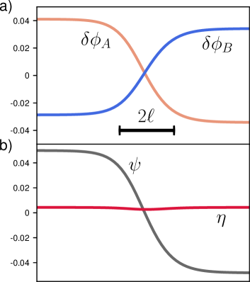
Figure 1: Example density profiles between coexisting phases for hard-spheres with $\alpha_{v}=27$ and $\alpha_{T}=20$ and $\epsilon_{\mathcal{A}}=\epsilon_{\mathcal{B}}=\beta_{\mathcal{B}}=8$ and hence $\tan\theta^{*}\approx 0.836$. We show a) profiles of the particle volume fractions $\delta\phi_{\mathcal{A}}=\phi_{\mathcal{A}}(z)-\phi_{\mathcal{A}}^{*}$ and $\delta\phi_{\mathcal{B}}=\phi_{\mathcal{B}}(z)-\phi_{\mathcal{B}}^{*}$, b) profiles of the normal coordinates $\psi(z)$ and $\eta(z)$; we observe that $\eta(z)\ll\psi(z)$. The interface width is $2\ell$ and away from the interface the densities take constant values at two coexisting phases.

IV.1 Surface tension

We consider a mixture with two phases at equilibrium and with a flat interface between the two phases. In this geometry, the two concentrations or the volume fractions vary only along one direction, say the $z$-direction so that $\partial_{y}c_{\alpha}=\partial_{x}c_{\alpha}=0$. The stress is isotropic in the bulk of each phase but becomes anisotropic close to the interface. The interfacial tension between the two phases can be calculated from the stress distribution in the solution

$$\gamma=\int_{z_{a}}^{z_{b}}(\sigma_{xx}-\sigma_{zz})dz$$ (26)

where the integration is from one phase (phase-$a$) to the other (phase-$b$). Using our calculated value of the stress tensor $\sigma_{ij}$, Eq. (15), we see that the isotropic component of the stress proportional to $\delta_{ij}$ cancels out and that only the non-diagonal components of the stress contribute to the surface tension: they vanish for $\sigma_{xx}$ but do not vanish for $\sigma_{zz}$. In dimensionless form, $\hat{\sigma}_{ij}\equiv v_{\mathcal{A}}T_{\mathcal{B}}^{-1}\sigma_{ij}$, we find

$$\hat{\sigma}_{xx}-\hat{\sigma}_{zz}=\hat{L}_{\mathcal{A}}(\partial_{z}\phi_{\mathcal{A}})^{2}+\hat{L}_{\mathcal{B}}(\partial_{z}\phi_{\mathcal{B}})^{2}$$

$$+2\hat{L}_{\mathcal{AB}}(\partial_{z}\phi_{\mathcal{A}})(\partial_{z}\phi_{\mathcal{B}})$$ (27)

In order to determine the surface tension $\gamma$ from Eqns (26) and  (27), we then need to determine the concentration profiles along $z$-direction. We first introduce the boundary conditions in the two phases in equilibrium: i) $\hat{\mu}_{\mathcal{A}}\left(\phi^{a}_{\mathcal{A}},\phi^{a}_{\mathcal{B}}\right)=\hat{\mu}_{\mathcal{A}}^{\dagger}=\hat{\mu}_{\mathcal{A}}\left(\phi^{b}_{\mathcal{A}},\phi_{\mathcal{B}}^{b}\right)$, ii) $\hat{\mu}_{\mathcal{B}}\left(\phi_{\mathcal{A}}^{a},\phi_{\mathcal{B}}^{a}\right)=\hat{\mu}_{\mathcal{B}}^{\dagger}=\hat{\mu}_{\mathcal{B}}\left(\phi_{\mathcal{A}}^{b},\phi^{b}_{\mathcal{B}}\right)$ and iii) $\hat{p}\left(\phi^{a}_{\mathcal{A}},\phi^{a}_{\mathcal{B}}\right)=\hat{p}^{\dagger}=\hat{p}\left(\phi_{\mathcal{A}}^{b},\phi_{\mathcal{B}}^{b}\right)$ where the values with daggers are the constant values of the chemical potentials and the pressure at equilibrium. The concentration profiles can then be calculated from the coupled differential equations:

$$\hat{\mu}_{\mathcal{A}}^{0}(z)-\hat{\mu}_{\mathcal{A}}^{\dagger}=\hat{L}_{\mathcal{A}}\nabla^{2}\phi_{\mathcal{A}}(z)+\hat{L}_{\mathcal{AB}}\nabla^{2}\phi_{\mathcal{B}}(z),$$ (28a)

$$\hat{\mu}_{\mathcal{B}}^{0}(z)-\hat{\mu}_{\mathcal{B}}^{\dagger}=\hat{L}_{\mathcal{B}}\nabla^{2}\phi_{\mathcal{B}}(z)+\hat{L}_{\mathcal{AB}}\nabla^{2}\phi_{\mathcal{A}}(z).$$ (28b)

Using the Gibbs-Duhem expression of the free energy in the phases at equilibrium, $\hat{f}^{0}=\hat{\mu}_{\mathcal{A}}^{0}\phi_{\mathcal{A}}+\hat{\mu}_{\mathcal{B}}^{0}\phi_{\mathcal{B}}-\hat{p}^{0}$ and integrating Eq.(28) is consistent with $\hat{\sigma}_{xx}-\hat{\sigma}_{zz}=\Delta\hat{f}\left[\phi_{\mathcal{A}}(z),\phi_{\mathcal{B}}(z)\right]$ where the tilted free energy is given by:

$$\Delta\hat{f}=\hat{f}-\left(\hat{\mu}_{\mathcal{A}}^{\dagger}\phi_{\mathcal{A}}+\hat{\mu}_{\mathcal{B}}^{\dagger}\phi_{\mathcal{B}}-\hat{p}^{\dagger}\right).$$ (29)

While this is the generic form, the same treatment more specifically implies that $\Delta\hat{f}=2\Delta\hat{f}^{0}$. The tilted free energy is the difference between the local free energy along the concentration profiles and the energy obtained from the so-called common tangent construction. Since the common tangent construction gives the minimal possible free energy, the tilted free energy is always positive $\Delta\hat{f}>0$ as long as one can solve the set of equations (28) with appropriate boundary conditions. We may therefore write an alternative form of the interfacial tension :

$$\hat{\gamma}\equiv T_{\mathcal{B}}^{-1}v_{\mathcal{A}}\gamma=2\int_{z_{a}}^{z_{b}}\Delta\hat{f}^{0}\left(\phi_{\mathcal{A}}(z),\phi_{\mathcal{B}}(z)\right)dz.$$ (30)

If there is a consistent profile, the surface tension $\gamma$ is therefore always positive and the interface between the two phases is stable. The set of equations (28) can be solved numerically by linearization of the two equations around one boundary (say phase $a$) and integrating up to the other boundary (phase $b$) using a shooting method. Alternatively, an analytical approximation can be obtained by considering the system close to the critical point as done in the next paragraph. This analytical approximation is in excellent agreement with the numerical results.

Surface tension near the critical point: In the vicinity of the critical point, we show in Appendix C how the effective thermodynamics can be expressed as a function of a single order parameter $\psi$ which is a linear combination volume fractions relative to the critical point. In addition, the other normal coordinate $\eta$ gives the normal distance from the critical point, and a phase separation occurs when a solution exists $\eta_{a}\approx\eta_{b}>0$. Each value of $\eta_{a}$ defines the two coexisting phases $\psi_{a}$ and $\psi_{b}$.The transformed coordinates are illustrated in Fig.1, where at first the concentration profiles $\phi_{\mathcal{A}}(z)$ and $\phi_{\mathcal{B}}(z)$ are obtained by solving Eq. (28) numerically. The effective tilted free energy density is given in (61) as a function of the order parameter only, which is obtained by transforming (29) to normal coordinates. Minimization with respect to $\psi$ leads to

$$\Delta\hat{f}^{0}=\frac{1}{4}{k_{\psi}}(\psi-\psi_{a})^{2}(\psi-\psi_{b})^{2}=\frac{1}{2}\hat{L}_{\psi}({\bf\nabla}\psi)^{2}.$$ (31)

Eqs.(30),(31) suggest that $\hat{\gamma}=\hat{L}_{\psi}\int(\nabla\psi)^{2}$, and hence the sign of $L_{\psi}$ determines the sign of the surface tension. It is then simple to prove that the surface tension for equal-sized hard spheres is positive for all $\alpha_{T}$ values. For hard spheres with varying size ratios, we checked by numerical evaluation of $L_{\psi}$ that it is positive for the values of the parameters $\alpha_{V}$ and $\alpha_{T}$ that lead to a phase separation except when $\alpha_{v}\ll 1$ or $\alpha_{v}\gg\alpha_{T}$ (see Appendix D for calculations, and Section V.2 for more discussion). The solution of (31) gives the concentration profile

$$\psi=\frac{\Delta\psi_{ab}}{2}\tanh z/\ell$$ (32)

where the interface width is $\ell=\left(\frac{8L_{\psi}}{{\Delta\psi_{ab}}^{2}k_{\psi}}\right)^{1/2}$. The surface tension can then be calculated by integration of Eq.(27) where we keep only the terms involving the gradient of $\psi$

$$\hat{\gamma}\approx\frac{1}{12}(\Delta\psi_{ab})^{3}\left(2k_{\psi}\hat{L}_{\psi}\right)^{1/2}.$$ (33)

In order to look at the scaling variation with parameters of the mixture such as $\alpha_{T}$ or $\alpha_{v}$, one must express the dimensionless quantities that we used as functions of these parameters. Taking as an example equal-sized hard spheres where $\alpha_{v}=1$, and hence $\alpha_{\zeta}=1$, $\epsilon_{\mathcal{A}}=\epsilon_{\mathcal{B}}=\beta_{\mathcal{B}}=8$, the volume fractions at the critical point are given by $\phi_{\mathcal{A}}^{*}=\alpha_{T}^{-1}$, $\phi_{\mathcal{B}}^{*}=1/8+(5/4)\alpha_{T}^{-1}$ when $\alpha_{T}\gg 1$. Considering a particle mixture of given volume fractions of particles (which could be called the laboratory conditions) $\phi_{\mathcal{A}}^{0}$ and $\phi_{\mathcal{B}}^{0}$ defined by $\phi_{\alpha}^{0}=V^{-1}\int_{V}\phi_{\alpha}({\bf r})d{\bf r}$ and for finite volume fractions in the vicinity of the critical point, we obtain:

$$\hat{\gamma}\sim(\phi_{\mathcal{A}}^{0})^{3/2}v_{0}^{1/3}\alpha_{T}^{3/2}$$ (34)

where $v_{0}$ is the volume of the particles . The real surface tension is then $\gamma=T_{\mathcal{B}}v_{0}^{-1}\hat{\gamma}$. The surface tension therefore increases as a power law of the ratio between the temperatures of the two types of particles $\alpha_{T}$ (see Appendix E for details).

IV.2 Kinetics of droplet growth

We consider a mixture quenched in the two phase region which is therefore supersaturated. We focus on a spherical droplet of phase-$b$ with radius $R$, growing inside the background phase which has a composition close to phase-$a$. The volume fractions outside the droplet are not equal to the concentrations in the $a$ phase due to the supersaturation, i.e., $\phi_{\mathcal{A}}\rightarrow\phi_{\mathcal{A}}^{a}+\delta\phi_{\mathcal{A}}$ and $\phi_{\mathcal{B}}\rightarrow\phi_{\mathcal{B}}^{a}+\delta\phi_{\mathcal{B}}$. Note that the concentrations inside the droplet are also slightly different from the concentrations of the $b$ phase but we can ignore this difference here.

This is a multi-scale problem with two well separated length scales: the width of the interface $\ell$ is much smaller than the droplet size $R$. At the scale of the small length $\ell$, the system is still close to equilibrium with chemical potentials $\hat{\mu}_{\mathcal{A}}^{\prime}$ and $\hat{\mu}_{\mathcal{B}}^{\prime}$ which are the chemical potentials slightly shifted from the phase equilibrium values and calculated outside the droplet on its surface. The steady-state equations, which give the particle concentration profiles are

$$\frac{\partial\hat{f}}{\partial\phi_{\mathcal{A}}}-\hat{\mu}_{\mathcal{A}}^{\prime}= \hat{L}_{\mathcal{A}}\left(\frac{\partial^{2}\phi_{\mathcal{A}}}{\partial r^{2}}+\frac{2}{r}\frac{\partial\phi_{\mathcal{A}}}{\partial r}\right)$$

$$+\hat{L}_{\mathcal{AB}}\left(\frac{\partial^{2}\phi_{\mathcal{B}}}{\partial r^{2}}+\frac{2}{r}\frac{\partial\phi_{\mathcal{B}}}{\partial r}\right),$$ (35)

$$\frac{\partial\hat{f}}{\partial\phi_{\mathcal{B}}}-\hat{\mu}_{\mathcal{B}}^{\prime}= \hat{L}_{\mathcal{B}}\left(\frac{\partial^{2}\phi_{\mathcal{B}}}{\partial r^{2}}+\frac{2}{r}\frac{\partial\phi_{\mathcal{B}}}{\partial r}\right)$$

$$+\hat{L}_{\mathcal{AB}}\left(\frac{\partial^{2}\phi_{\mathcal{A}}}{\partial r^{2}}+\frac{2}{r}\frac{\partial\phi_{\mathcal{A}}}{\partial r}\right).$$ (36)

In order to solve the so-called inner problem at the length scale $\ell$, we choose a length $\delta$ such that $\ell\ll\delta\ll R$. We multiply the first equation by $\partial\phi_{\mathcal{A}}/\partial r$ and the second one by $\partial\phi_{\mathcal{B}}/\partial r$, add them up and then integrate across the interface over a region of size $\delta$ such that in both phases, $\partial\phi_{\mathcal{A}}/\partial r=\partial\phi_{\mathcal{B}}/\partial r=0$ away from the interface. As a result, we obtain the Gibbs-Thomson relation Langer and Beenakker (1985) :

$$\delta\hat{\mu}_{\mathcal{A}}\Delta\phi_{\mathcal{A}}^{ab}+\delta\hat{\mu}_{\mathcal{B}}\Delta\phi_{\mathcal{B}}^{ab}=\frac{2\hat{\gamma}}{R}$$ (37)

where for each species, $\Delta\phi_{\alpha}^{ab}=\phi_{\alpha}^{b}-\phi_{\alpha}^{a}$ and $\delta\hat{\mu}_{\alpha}=\hat{\mu}_{\alpha}^{\dagger}-\hat{\mu}^{\prime}_{\alpha}$. Note that outside the droplet, as discussed below, the volume fractions and the chemical potentials vary over the large length scale $R$ and do not change over the length $\delta$. As in the previous section, we now transform the volume fractions to normal coordinates and obtain:

$$\delta\hat{\mu}_{\eta}\Delta\eta_{ab}+\delta\hat{\mu}_{\psi}\Delta\psi_{ab}=\frac{2\hat{\gamma}}{R}.$$ (38)

The non-critical variable $\eta$ is identical in the two phases so that $\Delta\eta_{ab}=0$. The small variation of the chemical potential $\delta\hat{\mu}_{\psi}$ can be obtained from Eq.(57) as $\delta\hat{\mu}_{\psi}\simeq 2k_{\psi}\psi_{a}^{2}\delta\psi$ using Eq.(60) where $\delta\psi=\psi(R)-\psi_{a}$ is the small shift of the order parameter on the surface of the droplet from its equilibrium value in phase-$a$. Then, rearranging Eq.(38), we have:

$$\delta\psi(R)=\frac{\hat{\gamma}}{Rk_{\psi}\psi_{a}^{2}\Delta\psi_{ab}}.$$ (39)

We now study the dynamics of the growing droplet by studying the outer problem, calculating the order parameter profile of the droplet material. As the non-critical variable $\eta$ has the same value in the two phases and as we find numerically that its variation is very small, we will assume here that there is no flux associated to this variable. The problem then has a single conserved order parameter $\psi$.

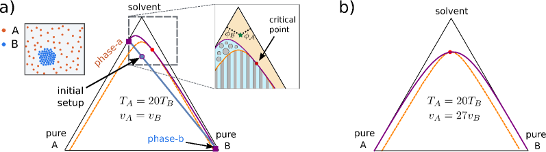
Figure 2: Triangular phase diagrams for three component system $\phi_{\mathcal{A}},\phi_{\mathcal{B}},\phi_{s}$(solvent) where $\phi_{\mathcal{A}}+\phi_{\mathcal{B}}+\phi_{s}=1$; for every point in the triangle the volume fractions are given by their distance from the facing triangle side (exemplified on scaled inset by star). Both diagrams are for hard-sphere systems ($a_{\alpha\beta}=0$, $\epsilon_{\mathcal{A}}=\epsilon_{\mathcal{B}}=8$) with temperature ratio $T_{\mathcal{A}}/T_{\mathcal{B}}=20$ while size ratios differ. In a) $v_{\mathcal{A}}=v_{\mathcal{B}}$ whereas in b) $v_{\mathcal{A}}=27v_{\mathcal{B}}$. The purple and dashed orange lines shows binodal and spinodal lines respectively and red dots are the critical points. The location of the critical point is asymmetric in both cases (though in opposite directions). Moreover, in a) we mark two coexisting phases $a$ and $b$ (purple squares) which are strongly asymmetric. Starting from the initial well-mixed setup, the system phase separates into a solid-like close-packed $\mathcal{B}$ particles (phase-$b$) surrounded by an $\mathcal{A}$ gas (phase-$a$) as illustrated in top left inset. In b) the phase diagram appears to be more symmetric indicating both liquid-like coexisting phases though shifted slightly towards $\mathcal{A}$-rich side. This results from having $\alpha_{T}/\alpha_{v}=20/27\lesssim 1$, the ratio which controls the symmetry of two phases (see Section III.4)

Outside the droplet, the order parameter $\psi$ follows a diffusion equation $\partial\psi/\partial t=D_{\psi}\nabla^{2}\psi$. We discuss the value of the effective diffusion constant $D_{\psi}$ in Appendix F. The boundary conditions for this diffusion equation are the value $\delta\psi(R)$ given by the Eq.(39) and the value at infinity $\psi_{\infty}$ which measures the supersaturation. The solution of the diffusion equation is

$$\psi(r)=\psi_{\infty}-(R/r)\left(\delta\psi_{\infty}-\delta\psi(R)\right).$$ (40)

The growth of the droplet is due to the radial flux $j_{\psi}=-D_{\psi}\frac{\partial\psi}{\partial r}|_{r=R}$ The conservation of the flux of the order parameter $\psi$ on the surface of the droplet leads to $\Delta\psi_{ab}\frac{dR}{dt}=D_{\psi}\frac{\partial\psi}{\partial r}|_{R}$. Inserting the solution of the diffusion equation, we obtain the evolution of the radius of the droplet

$$\frac{dR}{dt}=\frac{D_{\psi}}{R}\left(\Delta-\frac{d_{0}}{R}\right)$$ (41)

where the supersaturation is defined as $\Delta=\delta\psi(\infty)/\Delta\psi_{ab}$ and $d_{0}=\hat{\gamma}/(k_{\psi}\psi_{a}^{2}\Delta\psi_{ab}^{2})$ is a length of the order of the interfacial width $\ell$. This gives the critical nucleation radius of the droplet $R_{c}=d_{0}/\Delta$. Droplets smaller than $d_{0}$ collapse whereas droplets larger than $d_{0}$ grow.

At the early stages of the phase separation just after the quench, there are few droplets and the droplets that are larger than the critical radius grow as $R\sim t^{1/2}$. At long times, the value of the supersaturation decreases with time and a much more detailed analysis is required, which has been made by Lifshitz and Slyozov Lifshitz and Slyozov (1961). The supersaturation decreases as $\Delta\sim d_{0}/R$ and the average droplet radius increases as $R\sim t^{1/3}$. Plugging in the value of $D_{\psi}$ obtained in Appendix F gives the scaling of droplet growth with time, $R\sim(r_{G}t)^{1/3}$ in which the growth rate of mean droplet volume $r_{G}\sim(\phi_{\mathcal{A}}^{0}\alpha_{T})^{1/2}v_{0}^{1/3}T_{\mathcal{B}}/\zeta$ that is linearly proportional to the geometric mean of $T_{\mathcal{A}}$ and $T_{\mathcal{B}}$.

Here we obtain these power laws in the dilute limit of our two-temperature model (which can be mapped on an equilibrium system). On the other hand, at higher order in the density expansion even though the solution parameters ($\Delta,d_{0},D_{\psi},r_{G}$) change, there is no reason to expect a different power law behavior than $R\sim t^{1/3}$ as long as the droplet material is transported by diffusion. Similar examples include one component active fluids which respect the $1/3$ law Wittkowski et al. (2014); Lee (2017).

V Some applications of the theory

In this section, we show a few examples of application of the theory, to various systems. Some of these results are in accordance with existing numerical studies while some may motivate future experiments and simulations.

As discussed earlier, the intra- and inter-species interactions can be controlled either by modifying the interaction potentials between particles or by changing the activity difference (the temperature ratio). In the first case one alters the virial coefficients while in the latter case, one changes both the entropic part of the effective free energy by changing the temperatures $T_{\alpha}$ but also the weight of the interactions through the pairwise temperatures $T_{\alpha\beta}$ as seen in Eq. (10b). In general, for short-range interactions, the second virial coefficients can be written as $B_{\alpha\beta}\approx b_{\alpha\beta}+a_{\alpha\beta}/T_{\alpha\beta}$, where $b_{\alpha\beta}$ is the effective pair excluded volume and $a_{\alpha\beta}$ is the additional interaction part. Moreover, $b_{\alpha\beta}$ can be approximated by its hard-core value. As an example, for spherical particles, $b_{\alpha\beta}\approx(4\pi/3)d_{\alpha\beta}^{3}$ and $a_{\alpha\beta}\approx 4\pi\int_{d_{\alpha\beta}}^{\infty}u_{\alpha\beta}(r)r^{2}dr$ where $d_{\alpha\beta}$ is the distance between the centers of the particles at contact for an $\alpha\beta$ pair. If the additional interaction is purely attractive, $a_{\alpha\beta}<0$ is negative whereas it is positive if the additional interaction is repulsive. For a mixture of particles with given hard core sizes, this part of the virial coefficient can be tuned by chemical modifications. In addition, the contrast in activity which can be adjusted by the energy input per constituent, provides an extra handle Palacci et al. (2013); Theurkauff et al. (2012) for controlling the phase separation.

V.1 Colloidal hard spheres with different temperatures

Pure hard spheres interact with each other only through excluded volume interactions, which do not allow them to interpenetrate: $a_{\alpha\beta}=0$ and $B_{\alpha\beta}=b_{\alpha\beta}$. The dramatic influence of activity contrast towards demixing is clearly observed in mixtures of hard spheres with equal sizes and hence equal mobilities Weber et al. (2016). In Fig.2a we show the phase diagram for equal-sized hard spheres $\alpha_{v}=1,\ \alpha_{\zeta}=1$, then $\epsilon_{\mathcal{A}}=\epsilon_{\mathcal{B}}=\beta_{\mathcal{B}}=8$ with temperature ratio $\alpha_{T}=20$ . The volume fractions of the cold and hot particles are not equal at the critical point where the volume fraction of the cold particles is larger, indicating asymmetric phases. As exemplified in the phase diagram, starting from a mixture in the unstable region, the system phase separates into a solid-like close-packed $\mathcal{B}$ particles (phase-$\beta$, which is not quantitatively well described by our low density approximation) surrounded by an $\mathcal{A}$ gas (phase-$\alpha$) as illustrated by top left inset.

Using our formalism, we can also investigate the phase behavior of hard-sphere mixtures with different sizes. As we mentioned earlier, exclusively for active systems where $T_{\mathcal{A}}\neq T_{\mathcal{B}}$, do the mobilities (or the friction coefficients $\zeta_{\alpha}$) come into play via the effective pairwise temperature $T_{\mathcal{AB}}$ when $\zeta_{\mathcal{A}}\neq\zeta_{\mathcal{B}}$. For a given size ratio $\alpha_{v}$, $\beta_{\mathcal{B}}=(1+\alpha_{v}^{1/3})^{3}$ and using Stoke’s law $\alpha_{\zeta}=\alpha_{v}^{1/3}$. In Fig.2b we plot the phase diagram for mixtures of hard-spheres where the hot particles $\mathcal{A}$ are larger with a volume ratio $\alpha_{v}=27$ and a temperature ratio $\alpha_{T}=20$. The evolution of the phase diagram upon increasing the size ratio can be appreciated by comparison to equal-size hard-spheres at the same temperature ratio (Fig.2a-b). A more symmetrical phase diagram is predicted by increasing the volume ratio to reach $\alpha_{v}\approx\alpha_{T}$ and we expect coexistence between two liquid-like phases (Fig.2b). A further increase of size ratio shifts the phase diagram towards the $\mathcal{A}$-rich side as expected for mixtures of hard spheres with different sizes at the same temperature. Another way to observe the effect of tuning both size and temperature ratios is to evaluate the conditions required for the existence of a phase separation given in Section III.5 as a function of temperature and size ratios. We show this phase diagram in Fig. 3a which displays reenterances in both size ratio and temperature ratio axes.

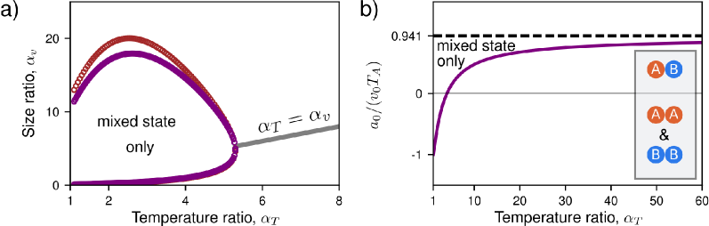
Figure 3: Control over mixing. a) Phase diagram for the existence of a phase separation in the temperature ratio $\alpha_{T}=T_{\mathcal{A}}/T_{\mathcal{B}}$ and volume ratio $\alpha_{v}=v_{\mathcal{A}}/v_{\mathcal{B}}$ plane for pure hard spheres. The purple line follows the spinodal condition while the outer brown boundary more strictly requires the existence of a critical point (see Section III.5). Inside these lines the solution remains mixed at all compositions. Interestingly, the phase diagram shows reentrance in both the lateral and vertical directions. The gray line $\alpha_{T}=\alpha_{v}$ separates the different regimes of phase compositions: i) on lower half-plane, we expect solid-like $\mathcal{B}$-rich phase and gas-like $\mathcal{A}$-rich phase, and ii) vice versa on upper half-plane, iii) whereas near the gray line we expect both liquid-like phases. In b) we use the same condition (in purple) for the existence of demixing for equal size hard spheres with short-range interactions of equal magnitude but opposing behavior (attractive vs. repulsive) for intra- and inter-species. The inset shows the favored interactions in both regimes. If $a_{0}>0$, the molecular interactions only promote mixing while at sufficiently large temperature ratios, the system can still reach phase separation.

V.2 Relation to active swimmers and active-passive particle mixtures

In dilute mixtures of active swimmers and passive particles, the run and tumble mechanism of the swimmers with propulsion speed $V_{\mathcal{A}}$ and reorientation time $\tau_{r}$ dictated by the time step between two tumbling events, can be considered at long times as entirely diffusive. If the reorientation time of swimmers is much smaller than the mean collision time (or mean free time), i.e., $\tau_{r}\ll\tau_{c}$, then $(T_{\mathcal{A}}-T_{\mathcal{B}})\approx P_{cs}\tau_{r}/3$ where $T_{\mathcal{B}}$ is the background temperature and $P_{cs}^{\mathcal{A}}=V_{\mathcal{A}}^{2}\zeta_{\mathcal{A}}$ is the mean power required to drive chemotaxis Mitchell (1991) for an active particle. Accordingly, keeping $\tau_{r}$ high will serve lower dissipation rate to maintain the same translational diffusivity. The validity range of this approximation in terms of the Péclet number $\text{Pe}=3V_{\mathcal{A}}\tau_{r}/d_{\mathcal{A}}$ where $d_{\mathcal{A}}$ is the diameter can be obtained by estimating $\tau_{c}$ for active swimmers Bruss and Glotzer (2018) using collision theory. It suggests that the effective diffusive approximation $(T_{\mathcal{A}}-T_{\mathcal{B}})\approx P_{cs}\tau_{r}/3$ remains valid for $\text{Pe}\ll\frac{3}{8\phi_{\mathcal{A}}}$ and density corrections are required as the concentration increases ($\tau_{r}\gg\tau_{c}$). Moreover, when we consider the emergence of the spinodal region as the demixing condition (Section III.5), we obtain at equal volume fractions $\phi_{\mathcal{A}}=\phi_{\mathcal{B}}=\phi_{s}$, the phase boundary follows $\phi_{s}\sim\text{Pe}^{-1}$. This relation is in accordance with simulations of mixtures of passive and active Brownian particles in two dimensions Stenhammar et al. (2015), although the simulations probe the phase separation at denser concentrations where both the diffusive approximation of the active swimmers fails (high Pe) and the dilute limit approximation of the phase separation theory is not qualitatively accurate.

One interesting aspect of our results is that we predict a positive surface tension as discussed in the previous section. In single component active fluids, the contribution from the swim pressure to the sign of surface tension is controversial. Certain approaches report negative Bialké et al. (2015), near zero Omar et al. (2020) or positive Hermann et al. (2019) values, or even supporting both Solon et al. (2018). For the two temperature model, at this order, the traditional ”effective” equilibrium route coincides with the mechanical framework, however, we discuss the breakdown of this construction on Section VI while going one order higher in density.

We can also express the cluster growth rate in terms of the mean power input. If the $\mathcal{A}$ and $\mathcal{B}$ constituents have the same volume $v_{0}$, at later stages of clustering, Eq.(72) suggests that the growth rate of mean cluster size $r_{G}\sim(\phi_{\mathcal{A}}P_{cs}\tau_{r})^{1/2}v_{0}^{1/3}T_{\mathcal{B}}^{1/2}/\zeta$ when $P_{cs}\gg T_{\mathcal{B}}/\tau_{r}$. This can be generalized similarly when there are two different types of swimmers and so on.

V.3 Interacting particles with different temperatures

Another interesting scenario appears when the interactions between particles enhance mixing while the activity contrast opposes and boosts demixing. To illustrate this scenario with an example, consider a system of particles with equal strength of interactions which are repulsive for identical particles and attractive between different particles. This could be achieved for example by mixing hot and cold particles of opposite net electric charges in a medium with a finite screening length. Similar other systems can be prepared by engineering chemical interactions. The interaction part of the virial coefficients can in this case be written as $a_{\mathcal{AA}}=a_{\mathcal{BB}}=a_{0}$ and $a_{\mathcal{AB}}=-a_{0}$. We may further simplify the problem by considering spherical particles of equal sizes such that $b_{\alpha\beta}=b_{0}=8v_{0}$ where $v_{0}$ is the molecular volume of the particles. We can evaluate the parameter range where a phase separation occurs. In Fig. 3b, we show the phase diagram in terms of the scaled interaction parameter $a_{0}/(T_{\mathcal{A}}v_{0})$, and the temperature ratio $\alpha_{T}=T_{\mathcal{A}}/T_{\mathcal{B}}$ for $T_{\mathcal{A}}>T_{\mathcal{B}}$. When $a_{0}>0$, the molecular interactions only promote mixing while at sufficiently large temperature ratios, the system can still reach phase separation.

V.4 Active-passive polymer blends

Biopolymers play a key role in intra-cellular or intra-nuclear organization in many instances Brangwynne et al. (2015), while they often interact with active proteins which confer them an active character. In our context, such activity in biopolymers has been shown to enhance spatial segregation and maintain compaction. This is the case for example displayed in the structure and compaction of DNA inside the cell nucleus Ganai et al. (2014); Nuebler et al. (2018). Similarly to colloidal particles, the active forces induce an effective temperature higher than the ambient one Osmanović and Rabin (2017). To give an example within our theory, we consider here a mixture of poly-$\mathcal{A}$ and poly-$\mathcal{B}$ chains in solution with equal lengths but with different temperatures (or activities) $T_{\mathcal{A}}>T_{\mathcal{B}}$ and having only excluded-volume interactions. For dilute solutions, one can still expect an effective thermodynamic behavior with an effective free energy given by a Flory-Huggins theory. In the spirit of the Flory-Huggins mean-field theory, we suppose here that the interaction part of the free energy does not depend on the connectivity between the monomers and that we can employ the results obtained for colloidal particles. Therefore, in order to describe the polymers, we use the chemical potentials obtained in the section II.1 by making the transformation $\mu_{\alpha}\rightarrow\mu_{\alpha}^{id}/N_{\alpha}+\Phi_{\alpha}$, where $N_{\alpha}$ is the number of monomers in each chain. Here, we consider the size interactions to be identical such that $\epsilon_{\mathcal{A}}=\epsilon_{\mathcal{B}}=\beta_{\mathcal{B}}=\epsilon_{0}$. By using the phase separation conditions described in Section III (both approaches agree in this case when $N_{\alpha}\gg 1$), we observe that segregation requires $(T_{\mathcal{A}}-T_{\mathcal{B}})/T_{\mathcal{B}}=\alpha_{T}-1>(2\epsilon_{0}^{-1/2})\left(N_{\mathcal{A}}^{-1/2}+N_{\mathcal{B}}^{-1/2}\right)$. This result agrees with extensive simulations of active-passive polymer mixtures Smrek and Kremer (2017) where the same scaling law is observed for $N_{\mathcal{A}}=N_{\mathcal{B}}=N$ as the condition becomes $\alpha_{T}-1>(4\epsilon_{0}^{-1/2})N^{-1/2}$, though in terms of effective temperatures. Our mean-field exponents on the profile $\Delta\psi\sim\alpha_{T}^{1/2}$, and interface width $\ell\sim\alpha_{T}^{-1/2}$ seem close to the values obtained from simulations by the same authors in Ref.Smrek and Kremer (2018).

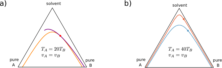
Figure 4: Evolution of triangular phase diagrams by third order contributions. The presentation on how to read the components in the phase diagrams is given in caption of Figure 2. In a) we only show the resulting phase diagram obtained using third-order expansion where we display binodal (purple), spinodal (orange dashed) lines and the critical point (red) for equal-sized hard spheres with $T_{\mathcal{A}}/T_{\mathcal{B}}=20$. In b) we compare the spinodal lines and the critical points (for clarity, not the binodals) obtained from second-order (orange) and third-order (light blue) expansions for equal-sized hard spheres with $T_{\mathcal{A}}/T_{\mathcal{B}}=40$.

VI Higher order expansions in concentration

VI.1 General form

Up to this point, we have studied the general phase behavior of a suspension of mixed particles with different temperatures in the dilute limit. In this limit, the theory takes into account only two-particle correlations, the system has an effective thermodynamic description and the phase behavior can be obtained from the direct analog of the equilibrium construction of phase separation, despite the existence of non-equilibrium aspects such as the violation of detailed balance that are observed at the microscopic level Grosberg and Joanny (2015). A natural extension of this approach is then to calculate higher order corrections in concentration and see whether the effective thermodynamic description is preserved.

In order to answer this question, we must first obtain the steady-state pair distribution function $g_{\alpha\beta}^{ss}({\bf r}_{1}-{\bf r}_{2})$ at next orders in particle densities $c_{\alpha}$. A general strategy would be to start from the Fokker-Planck equation (II) for the multi-particle probability distribution $P$, and integrate up to the desired order in densities. One can then solve the remaining coupled equations to obtain the pair distribution functions $g_{\alpha\beta}^{ss}({\bf r}_{1}-{\bf r}_{2})$. This approach leads to the Bogoliubov-Born-Green-Kirkwood-Yvon (BBGKY) hierarchy Hansen and McDonald (1995). For our problem, a non-equilibrium analog of this hierarchy is detailed in Ref. Grosberg and Joanny (2015). In the equilibrium case, the fluxes vanish and the distribution functions are found by imposing a closure relation. By contrast, in a non-equilibrium case, for $T_{\mathcal{A}}\neq T_{\mathcal{B}}$, there might exist non-vanishing fluxes associated to dissipation in the system . This complication makes it difficult to obtain a systematic expansion at higher orders in densities.

A solvable example of Fokker-Planck equation (or the Langevin dynamics) at higher order has been given for pairwise harmonic potential interactions. In this case, a steady-state solution exists Wang and Grosberg (2020) for $\sum_{m}\partial_{m}J_{m}=0$ while the fluxes $J_{m}\neq 0$ when $T_{\mathcal{A}}\neq T_{\mathcal{B}}$. As a result, it is not possible to formulate a solution in Boltzmann form with a scalar temperature.

Other classical approaches such as the Kirkwood superposition approximation would also fail. We refer the reader to the probabilistic interpretation of the Kirkwood closure in Ref.Singer (2004). Nevertheless, in the following section, we demonstrate an alternative approach based on the calculation of depletion forces, to obtain third-order density corrections for pure hard-sphere interactions.

VI.2 Hard spheres

In the case of mixtures with only hard-sphere interactions, an appropriate approach to expand at least to the next order, considers the depletion interaction between two particles due to a third particle Asakura and Oosawa (1958). This method has been used repeatedly in colloid science Mao et al. (1995) and recovers exactly the third virial coefficients in hard-sphere mixtures with different radii. The full details of the calculation are given in Appendix G. Here as an example, we briefly sketch the results obtained for equal-sized hard-spheres with different temperatures. The method is also applicable to particles of differing size ratios as shown in the Appendix G. The resulting pressure is given by the standard virial expansion:

$$p^{0}=\sum_{\alpha}T_{\alpha}c_{\alpha}+\frac{B}{2}\sum_{\alpha,\beta}T_{\alpha\beta}c_{\alpha}c_{\beta}+C\sum_{\alpha,\beta,\gamma}T_{\gamma}c_{\gamma}c_{\alpha}c_{\beta}$$ (42)

where $B$ and $C$ are the second and third virial coefficients respectively, which are identical for all types of pairs and triplets of particles and $\alpha,\beta,\gamma=\mathcal{A}$ or $\mathcal{B}$.

In equilibrium systems, there is a direct route from pressure to chemical potentials using the Gibbs-Duhem equation $p_{0}=\sum_{\alpha}\mu_{\alpha}^{0}c_{\alpha}-f^{0}$, where the chemical potentials are given by $\mu_{\alpha}^{0}=\partial f^{0}/\partial c_{\alpha}$. Our analysis for systems with two temperatures has shown that this remains applicable in the dilute limit approximation. However, without knowing explicitly the effective free energy, this approach is not founded. Thus, one should always start from the dynamic equations for the concentrations. If we insist in rewriting the interaction part of the chemical potentials defined in Eq. (8) as a series expansion in densities $\Phi_{\alpha}=\Phi_{\alpha}^{(1)}+\Phi_{\alpha}^{(2)}$, we only obtain the value of the chemical potential gradient at second order in the densities:

$$\begin{split}\nabla\Phi_{\mathcal{A}}^{(2)}=&C\bigg{[}\nabla\left(\frac{3}{2}T_{\mathcal{A}}c_{\mathcal{A}}^{2}+\frac{3}{2}T_{\mathcal{B}}c_{\mathcal{B}}^{2}\right)\\ &+\left(2T_{\mathcal{B}}+T_{\mathcal{A}}\right)c_{\mathcal{B}}\nabla c_{\mathcal{A}}+\left(2T_{\mathcal{A}}+T_{\mathcal{B}}\right)c_{\mathcal{A}}\nabla c_{\mathcal{B}}\bigg{]}\end{split}$$ (43)

where $C$ is the third virial coefficient between hard spheres of the same size (see Appendix G), which is equal for all types of interactions. At this order, $\nabla\Phi_{\mathcal{B}}^{(2)}=\nabla\Phi_{\mathcal{A}}^{(2)}$ because the mixture contains particles of equal sizes. The total chemical potentials $\mu_{\alpha}^{(2)}=\mu_{\alpha}+\Phi_{\alpha}^{(2)}$ are then obtained from Eqs. (9), (43). However, the gradient $\nabla\Phi_{\alpha}^{(2)}$ given by Eq. (43) is non-integrable to a potential function due to the mismatch between the cross terms. This incompatibility is related to the non-equilibrium character of solutions of particles at different temperatures and hence the mismatch vanishes for an equilibrium solution, when $T_{\mathcal{A}}=T_{\mathcal{B}}$. As a result, the non-equilibrium additional terms break down the routes to construct an effective thermodynamic theory. A similar breakdown has been previously observed in one component active fluids with density-dependent motilities Wittkowski et al. (2014) where the interfacial contributions lead to terms not integrable to a free energy. That issue has then been addressed in Ref. Solon et al. (2018), by introducing a functional transformation using an alternative scalar order parameter. By contrast, here we are not able to define even the local chemical potentials at third order in the dynamical equations  (6), (7). This could as well indicate the existence of bubbly phases Tjhung et al. (2018) in which two steady state phases exist only locally and are separated by interfaces. A more detailed study would require to extend the analysis in gradient terms presented in the previous sections. We plan to address this question in a further study.

Since the term $\nabla\Phi_{\mathcal{A}}^{(2)}$ is not integrable to a chemical potential form, it is not straightforward to determine all uniformly conserved quantities at the zero-flux steady-state. At phase equilibrium, we only find two conserved quantities since $\nabla p^{0}=0$ and $\nabla(\mu_{\mathcal{A}}^{0}-\mu_{\mathcal{B}}^{0})=0$. The latter condition exists specifically for equal-sized hard-spheres, because $\nabla\Phi_{\mathcal{B}}^{(2)}=\nabla\Phi_{\mathcal{A}}^{(2)}$. A third condition however, can be obtained by linearization of one of the concentration fluxes around the critical point. Then, the calculated phase diagrams are shown in Fig.4 in comparison to the phase diagram obtained from the previous expansion using second order virial coefficients (dilute limit) for the same set of parameters $\alpha_{v}=1$, $\alpha_{T}=40$. Curiously, the contribution from the third order terms delays the onset of demixing. We also observe that the instability occurs in physical region of the phase diagram for temperature ratios $\alpha_{T}>6.171$, not very far from the value obtained using second order analysis, i.e., $\alpha_{T}>4$ Note (2).

VII Conclusion

To summarize, in this work, we have outlined the general framework to study the characteristics of phase equilibria in active mixtures of diffusive type where the temperatures of the constituents are different. We obtain the phase diagrams and phase growth properties using two methods in parallel which cover both the equilibrium thermodynamic description through functional analysis and a more general approach considering steady-state solutions of the Fokker-Planck equations. For each observable and method, we compare and contrast the non-equilibrium $T_{\mathcal{A}}\neq T_{\mathcal{B}}$ scenarios to the equilibrium ones $T_{\mathcal{A}}=T_{\mathcal{B}}$. This allows us to reexplore landmark methods and concepts developed to establish the foundational principles of equilibrium solution theory. Resemblances appear in the steady-state solutions while the non-equilibrium state when $T_{\mathcal{A}}\neq T_{\mathcal{B}}$ is only maintained with a net power dissipation. Even though these systems have a non-equilibrium character, it turns out that they recover a direct analog of the equilibrium construction in the dilute limit. Within this approximation, the direct connection with the equilibrium thermodynamics is linked to the closure of the hierarchy of correlation functions,which imposes a vanishing flux along the coordinate of interactions (the separation vector) for all two-body clusters (while this is no longer true for higher order clusters). In this dilute limit, we were able to construct a Cahn-Hilliard theory generalized to two temperature mixtures. This also validates a reasonable ground for phenomenological studies considering active systems as a perturbation around an equivalent equilibrium dynamics.

The analog of the equilibrium picture provides a rich palette to explore various aspects of active/passive (or less active) mixtures. In this case, the activity differences between the particles, introduce another level of control on the phase separation properties. As we demonstrate by examples, the theory has broad applications in diverse physical systems at different length scales. We have also introduced a transformation to normal coordinates around the critical state where the phase dynamics can be described by a single critical order parameter. We obtain counterparts of mean-field exponents of profile parameter $\psi$ to express interfacial properties, while $\eta$ becomes a measure of normal distance from the critical point (Similar to the temperature direction in regular solutions Cahn and Hilliard (1958); Bray (2002), but not exactly the same since $\eta\equiv\eta(z)$ is a slightly varying function of $z$ along the interface). In this simplified formalism, we capture interesting scaling laws for interfacial properties, droplet growth dynamics, and for the phase segregation condition. We observe that the surface tension is always positive at the interface of two phases for binary mixtures of equal-sized hard spheres. Some of our results are in agreement with existing numerical simulations (detailed in Section V). Our results also suggest a means to calibrate the composition of coexisting phases (liquid-liquid vs. gas-like and solid-like) by controlling the ratio $\alpha_{T}/\alpha_{v}$ which could motivate experimental applications.

Higher order corrections (though not available for the general case) break down the direct analogy with the equilibrium construction in the case of pure hard-core interactions. However, the results do not indicate significant qualitative differences with the equilibrium behavior, and hence in general, the qualitative behavior of the system should be obtained from the simpler theory describing the dilute limit (Sections II-IV) that gives an intuitive understanding of demixing in diffusive systems. On the other hand, the existence of non-local terms in the chemical potentials at the third order in a power expansion in densities might indicate the emergence of new phenomena. It would be interesting to study these cases further including inhomogeneous terms, in order to bridge the gap between microscopic and coarse-grained models Solon et al. (2018); Tjhung et al. (2018).

Appendix A Solution of the two-particle Fokker-Planck equation

By evaluating Eq. (II) for only two-particles $\alpha$ and $\beta$ at positions ${\bf r}_{1}$ and ${\bf r}_{2}$, and introducing a pairwise potential which depends only on the distance between these particles, $u_{\alpha\beta}\equiv u_{\alpha\beta}\left(|{\bf r}_{1}-{\bf r}_{2}|\right)$ such that $\partial_{{\bf r}_{1}}u_{\alpha\beta}=-\partial_{{\bf r}_{2}}u_{\alpha\beta}$, we can derive the steady-state solution using separation of variables where $\alpha,\beta=\mathcal{A}$ or $\mathcal{B}$. Accordingly, we set the two-particle probability function $P_{\alpha\beta}\equiv G_{\alpha\beta}({\bf R})g_{\alpha\beta}({\bf r})$ where ${\bf r}={\bf r}_{2}-{\bf r}_{1}$ is the separation vector and ${\bf R}=\tau_{\alpha}{\bf r}_{1}+\tau_{\beta}{\bf r}_{2}$ is the center of motion with $\tau_{\alpha}=\zeta_{\alpha}T_{\beta}/(\zeta_{\alpha}T_{\beta}+\zeta_{\beta}T_{\alpha})$ such that the diffusions along ${\bf r}$ and ${\bf R}$ are statistically independent Grosberg and Joanny (2015). As a result, we obtain:

$$\frac{\partial P_{\alpha\beta}}{\partial t}=-\partial_{r}J_{r}^{\alpha\beta}-\partial_{R}J_{R}^{\alpha\beta}$$ (44)

with flux components:

$$J_{r}^{\alpha\beta} =\begin{aligned} &-\left(\frac{\zeta_{\alpha}+\zeta_{\beta}}{\zeta_{\alpha}\zeta_{\beta}}\right)\frac{\partial u_{\alpha\beta}}{\partial{\bf r}}P_{\alpha\beta}\\ &-\left(\frac{\zeta_{\alpha}T_{\beta}+\zeta_{\beta}T_{\alpha}}{\zeta_{\alpha}\zeta_{\beta}}\right)\frac{\partial P_{\alpha\beta}}{\partial{\bf r}}\end{aligned}$$ (45)

$$J_{R}^{\alpha\beta} =\begin{aligned} &-\left(\frac{T_{\alpha}-T_{\beta}}{\zeta_{\alpha}T_{\beta}+\zeta_{\beta}T_{\alpha}}\right)\frac{\partial u_{\alpha\beta}}{\partial{\bf r}}P_{\alpha\beta}\\ &-\left(\frac{T_{\alpha}T_{\beta}}{\zeta_{\alpha}T_{\beta}+\zeta_{\beta}T_{\alpha}}\right)\frac{\partial P_{\alpha\beta}}{\partial{\bf R}}.\end{aligned}$$ (46)

Setting the flux $J_{r}=0$ for the steady-state solution results Eq.(4) in the main text. The remaining part only requires a uniform $G({\bf R})$ which satisfies the steady-state solution though $J_{R}^{\alpha\beta}$ does not necessarily vanish for $T_{\alpha}\neq T_{\beta}$ .

Appendix B Irving-Kirkwood method for calculation of internal stress

Following the stress equation for the interaction part, Eq.(18) in the main text up to second order in separation vector ${\bf r}$ while using Eq.(4) and keeping only non-vanishing terms upon integration, we rewrite the internal stress $\sigma_{ij}^{(v)}$ given by Eq. (17) as:

$$\begin{split}\sigma_{ij}^{(v)}=-p_{0}\delta_{ij}+\sum_{\alpha,\beta}&\frac{T_{\alpha\beta}}{2}\int\bigg{[}\frac{r_{i}r_{j}}{{\bf r}}\frac{\partial}{\partial r}\left(1-e^{-u_{\alpha\beta}(r)/T_{\alpha\beta}}\right)\\ &\bigg{(}\frac{1}{6}({\bf r}\cdot\nabla)^{2}c_{\alpha}({\bf r}_{1})c_{\beta}({\bf r}_{1})\\ &-\frac{1}{2}[{\bf r}\cdot\nabla c_{\alpha}({\bf r}_{1})][{\bf r}\cdot\nabla c_{\beta}({\bf r}_{1})]\bigg{)}\bigg{]}d{\bf r},\end{split}$$ (47)

where $p^{0}=\left(\mu^{0}_{\mathcal{A}}c_{\mathcal{A}}+\mu^{0}_{\mathcal{B}}c_{\mathcal{B}}-f^{0}\right)$ is the locally uniform pressure. Integrating by parts gives:

$$\begin{split}\sigma_{ij}^{(v)}=-p_{0}\delta_{ij}+\sum_{\alpha,\beta}\frac{T_{\alpha\beta}}{2}\mathcal{I}_{ijkl}&\bigg{[}\frac{1}{12}\left(\partial_{k}c_{\alpha}\partial_{l}c_{\beta}+\partial_{k}c_{\beta}\partial_{l}c_{\alpha}\right)\\ &-\frac{1}{6}\left(c_{\alpha}\partial_{k}\partial_{l}c_{\beta}+c_{\beta}\partial_{k}\partial_{l}c_{\alpha}\right)\bigg{]}\end{split}$$ (48)

where a summation on the $k,l$ indices is performed using an Einstein summation convention, and the integral $\mathcal{I}_{ijkl}$ is given by:

$$\mathcal{I}_{ijkl}=\int\frac{r_{i}r_{j}r_{k}r_{l}}{r^{2}}\left(1-e^{-u_{\alpha\beta}(r)/T_{\alpha\beta}}\right)d{\bf r}.$$ (49)

Considering the symmetries and performing the sum, we finally reach an expression for the difference between stress obtained by two different methods:

$$\begin{split}\sigma_{ij}^{(v)}-\sigma_{ij}=\sum_{\alpha,\beta}L_{\alpha\beta}\bigg{[}-\frac{1}{3}\nabla^{2}\left(c_{\alpha}c_{\beta}\right)\delta_{ij}+\frac{1}{3}\partial_{i}\partial_{j}\left(c_{\alpha}c_{\beta}\right)\bigg{]}\end{split}$$ (50)

where $\sigma_{ij}$ is the result obtained by free energy deformation given in Eq. (15). Summing over $\alpha,\beta$ suggests that the addition of the gauge term discussed in Section II.2, i.e., $-\frac{1}{3}\nabla^{2}\left[L_{\mathcal{A}}c_{\mathcal{A}}^{2}+2L_{\mathcal{AB}}c_{\mathcal{A}}c_{\mathcal{B}}+L_{\mathcal{B}}c_{\mathcal{B}}^{2}\right]$ to the original free energy $f$, leads back to the Irving-Kirkwood formula.

Appendix C Transformation of order parameters to normal coordinates around the critical point

Close to the critical point $\{\phi_{\mathcal{A}}^{*},\phi_{\mathcal{B}}^{*}\}$, the effective thermodynamic description becomes simpler if instead of using the volume fractions measured with respect to the volume fractions at the critical point $\delta\phi_{\alpha}=\phi_{\alpha}-\phi_{\alpha}^{*}$ as variables, we make a linear transformation to the eigenvectors of the inverse compressibility matrix $\kappa^{-1}_{p}$ at the critical point. The inverse compressibility matrix is a symmetric matrix given by Eq. (23) and it can be written as

$$\kappa^{-1}_{p}=\left(\begin{matrix}c+a&b\\ b&c-a\end{matrix}\right)$$ (51)

The values of the coefficients are given by Eq.(23) $c=\frac{1}{2}\left[\alpha_{T}\left(\frac{1+\epsilon_{\mathcal{A}}\phi_{\mathcal{A}}}{\phi_{\mathcal{A}}}\right)+\alpha_{v}\left(\frac{1+\epsilon_{\mathcal{B}}\phi_{\mathcal{B}}}{\phi_{\mathcal{B}}}\right)\right]$, $a=\frac{1}{2}\left[\alpha_{T}\left(\frac{1+\epsilon_{\mathcal{A}}\phi_{\mathcal{A}}}{\phi_{\mathcal{A}}}\right)-\alpha_{v}\left(\frac{1+\epsilon_{\mathcal{B}}\phi_{\mathcal{B}}}{\phi_{\mathcal{B}}}\right)\right]$ and $b=\frac{\alpha_{T}+\alpha_{\zeta}}{1+\alpha_{\zeta}}\beta_{\mathcal{B}}$. We denote the two eigenvalues of the matrix by $\epsilon$ and $\lambda$. The coefficients of the matrix are real and related to the eigenvalues by $c=\frac{\lambda+\epsilon}{2}$ and $(a^{2}+b^{2})^{1/2}=\frac{\lambda-\epsilon}{2}$. In the vicinity of the critical point, $\epsilon$ is small and vanishes as one approaches the critical point and the other eigenvalue $\lambda$ remains finite at the critical point. The eigenvector associated with $\epsilon=0$ at the critical point, gives the direction in which the fluctuations diverge. We also define an angle $\theta$ such that $a=-\frac{\lambda-\epsilon}{2}\cos 2\theta$ and $b=\frac{\lambda-\epsilon}{2}\sin 2\theta$. The diagonalization appears then as a rotation of angle $\theta$ and the eigenvalue matrix $D_{\epsilon,\lambda}$ with diagonal entries $\epsilon$ and $\lambda$ is obtained by rotation to the basis of eigenvectors $D_{\epsilon,\lambda}=R(\theta)\kappa^{-1}_{p}R^{T}(\theta)$ using the standard rotation matrix $R(\theta)$.

In the volume fraction space, the eigenvectors are obtained using a rotation of the natural coordinates by an angle $\theta$. The normal coordinates that we use are the coordinates along the eigenvectors of the inverse compressibility matrix at the critical point. At the critical point, the rotation angle of the eigenvectors is $\theta^{*}$ that satisfies

$$\tan\theta^{*}=\frac{b^{*}}{c^{*}-a^{*}}=\frac{(\alpha_{T}+\alpha_{\zeta})\beta_{\mathcal{B}}\phi_{\mathcal{B}}^{*}}{\alpha_{v}(1+\alpha_{\zeta})(1+\epsilon_{\mathcal{B}}\phi_{\mathcal{B}}^{*})}$$ (52)

which can also be expressed in conjugate form in terms of $\phi_{\mathcal{A}}^{*}$ using $\tan\theta^{*}=\frac{c^{*}+a^{*}}{b^{*}}$. This angle gives the orientation of the tie lines close to the critical point. As a result, it provides an indication on the asymmetry of composition between the two phases. Thus, when $\tan\theta^{*}\approx 1$ , we would have two liquid-like phases, whereas for $\tan\theta^{*}\gg 1$, the critical point is towards $\mathcal{B}$-rich side of the phase diagram with a solid-like and a gas-like phase coexisting and vice versa for $\tan\theta^{*}\ll 1$.

In the eigenbasis of the inverse compressibility matrix at the critical point, there is a coordinate $\psi$ along the eigenvector associated to the vanishing eigenvalue and a coordinate $\eta$ along the eigenvector associated to the finite eigenvalue $\lambda$. These two normal coordinates are related to the original volume fractions by the rotation matrix $R(\theta^{*})$. Accordingly, we define:

$$\left(\begin{matrix}\psi\\ \eta\end{matrix}\right)=R(\theta^{*})\left(\begin{matrix}\delta\phi_{\mathcal{A}}\\ \delta\phi_{\mathcal{B}}\end{matrix}\right).$$ (53)

The coordinate $\psi$ is the critical variable that we call the order parameter. Along these new coordinates, differentiation is performed as:

$$\left(\begin{matrix}\frac{\partial}{\partial\psi}\\ \frac{\partial}{\partial\eta}\end{matrix}\right)=R(\theta^{*})\left(\begin{matrix}\frac{\partial}{\partial\phi_{\mathcal{A}}}\\ \frac{\partial}{\partial\phi_{\mathcal{B}}}\end{matrix}\right).$$ (54)

Using these relations, we expand the free energy around the critical point and obtain:

$$\hat{f}_{0}=\hat{f}_{0}^{*}+\hat{\mu}_{\eta}^{*}\eta+\hat{\mu}_{\psi}^{*}\psi+\frac{k_{2}}{2}\psi^{2}\eta+\frac{k_{4}}{4}\psi^{4}+\frac{\lambda^{*}}{2}\eta^{2},$$ (55)

where the coefficients of the expansion are the derivatives of the free energy $\hat{f}_{0}$ evaluated at the critical point: $k_{2}=\frac{\partial^{3}\hat{f}_{0}}{\partial\psi^{2}\partial\eta}\Big{|}_{*}$, $k_{4}=\frac{1}{3!}\frac{\partial^{4}\hat{f}_{0}}{\partial\psi^{4}}\Big{|}_{*}$, $\lambda^{*}=\frac{\partial^{2}\hat{f}_{0}}{\partial\eta^{2}}\Big{|}_{*}$ and we used the fact that $\eta$ is a slowly changing variable. The Hessian matrix of the second derivatives of the free energy is equal to the inverse compressibility matrix. In the coordinates $\psi,\eta$ the inverse compressibility matrix is $D_{\epsilon,\lambda}$ evaluated at the critical point where $\epsilon=0$. The two derivatives $\frac{\partial^{2}\hat{f}_{0}}{\partial\psi\partial\eta}\Big{|}_{*}$ and $\frac{\partial^{2}\hat{f}_{0}}{\partial\psi^{2}}\Big{|}_{*}$ therefore vanish. The third derivative of the free energy $\frac{\partial^{3}\hat{f}_{0}}{\partial\psi^{3}}\Big{|}_{*}$ also vanishes because $\psi$ is the tangent direction to the spinodal line at the critical point. The two chemical potentials along the new coordinates are obtained again by differentiation of the free energy $\hat{f}_{0}$:

$$\hat{\mu}_{\eta} = \hat{\mu}_{\eta}^{*}+\lambda^{*}\eta+k_{2}\frac{\psi^{2}}{2}$$ (56)

$$\hat{\mu}_{\psi} = \hat{\mu}_{\psi}^{*}+k_{2}\eta\psi+{k_{4}}\psi^{3}$$ (57)

The coordinates of the equilibrium phases $a$ and $b$ (the binodal line) are obtained by equating the chemical potentials $\hat{\mu}_{\psi}$ and $\hat{\mu}_{\eta}$ and the pressure in the two phases. This leads to $\eta_{a}=\eta_{b}$ and $\psi_{a}^{2}=\psi_{b}^{2}=-\frac{k_{2}}{k_{4}}\eta_{a}$. By construction of the normal coordinates, the tie lines, which are the straight lines joining the two phases at equilibrium correspond to lines of constant values of $\eta$. The binodal line has therefore a parabolic shape with $\psi_{a}\approx-\psi_{b}$. Each value of $\eta_{a}\approx\eta_{b}>0$ defines the coexisting phases $\psi_{a}$ and $\psi_{b}$. It is convenient in the following to consider a symmetrized version of the order parameter $\Delta\psi_{ab}=\psi_{b}-\psi_{a}$, which satisfies $\Delta\psi_{ab}^{2}=-\frac{4k_{2}}{k_{4}}\eta_{a}$.

The total free energy density is obtained by including the gradient terms which also can be transformed to the normal coordinates. In the vicinity of the critical point, as the non-critical variable $\eta$ is much smaller than the order parameter $\psi$ we only need to retain terms in $({\bf\nabla}\psi)^{2}$. The total free energy density reads then

$$\hat{f}=\hat{f}_{0}+\frac{\hat{L}_{\psi}}{2}({\bf\nabla}\psi)^{2}$$ (58)

where the coefficient $\hat{L}_{\psi}$ is given by $\hat{L}_{\psi}={\hat{L}}_{\mathcal{A}}\cos^{2}\theta^{*}-2{\hat{L}}_{\mathcal{AB}}\cos\theta^{*}\sin\theta^{*}+{\hat{L}}_{\mathcal{B}}\sin^{2}\theta^{*}$.

In order to calculate the interfacial tension, we must define the two phases at equilibrium i.e. fix the values $\eta_{a}$ in the two phases in equilibrium. This also fixes the order parameter $\Delta\psi_{ab}$. We must then calculate what we called the tilted free energy around the critical point

$$\Delta\hat{f}[\psi,\eta]=\hat{f}[\psi,\eta]-\hat{f}^{0}(\psi_{a},\eta_{a})-\hat{\mu}_{\psi}^{\dagger}\left(\psi-\psi_{a}\right)-\hat{\mu}_{\eta}^{\dagger}\left(\eta-\eta_{a}\right)$$ (59)

The constants $\hat{\mu}_{\psi}^{\dagger}$ and $\hat{\mu}_{\eta}^{\dagger}$ are the chemical potentials calculated in the two phases at equilibrium. Note that the tilted free energy has a minimum and vanishes in the two phases in equilibrium. The profiles of $\psi$ and $\eta$ as a function of the coordinate $z$ perpendicular to the interface are obtained by minimization of the tilted free energy. We first minimize the tilted free energy with respect to $\eta$. This leads to

$$\eta=\eta_{a}-\frac{k_{2}}{2\lambda^{*}}(\psi^{2}-{\psi_{a}}^{2}).$$ (60)

Inserting this result into the tilted free energy, we obtain the tilted free energy as a function of the order parameter $\psi$ only, which we write as

$$\Delta\hat{f}(\psi)=\frac{k_{\psi}}{4}(\psi-\psi_{a})^{2}(\psi-\psi_{b})^{2}+\frac{\hat{L}_{\psi}}{2}({\bf\nabla}\psi)^{2}$$ (61)

where $k_{\psi}=k_{4}-\frac{k_{2}^{2}}{2\lambda^{*}}$. This free energy is minimal and vanishes at $\psi=\psi_{a}$ and $\psi=\psi_{b}$. Finally, minimization with respect to $\psi$ yields:

$$\Delta\hat{f}^{0}(\psi)=\frac{k_{\psi}}{4}(\psi-\psi_{a})^{2}(\psi-\psi_{b})^{2}=\frac{\hat{L}_{\psi}}{2}({\bf\nabla}\psi)^{2}$$ (62)

which shows that along the order parameter profile between the two phases, $\Delta\hat{f}(\psi)=2\Delta\hat{f}^{0}(\psi)$.

Appendix D Positivity of the surface tension

As mentioned in the main text, since $\hat{\gamma}=L_{\psi}\int(\nabla\psi)^{2}$ integrated from one phase to the other, the sign of $L_{\psi}$ determines the sign of the surface tension. We can determine the sign of $L_{\psi}$ using our results in Section II. From the definition $\hat{L}_{\psi}={\hat{L}}_{\mathcal{A}}\cos^{2}\theta^{*}-2{\hat{L}}_{\mathcal{AB}}\cos\theta^{*}\sin\theta^{*}+{\hat{L}}_{\mathcal{B}}\sin^{2}\theta^{*}$, the positivity of surface tension requires:

$$2\tan\theta^{*}-\frac{{\hat{L}}_{\mathcal{A}}}{{\hat{L}}_{\mathcal{AB}}}-\frac{{\hat{L}}_{\mathcal{B}}}{{\hat{L}}_{\mathcal{AB}}}\tan^{2}\theta^{*}>0.$$ (63)

We have previously defined rescaled parameters $\hat{L}_{\alpha\beta}=T_{\mathcal{B}}^{-1}L_{\alpha\beta}v_{\mathcal{A}}/(v_{\alpha}v_{\beta})$ on Section III.A (then $\hat{L}_{\mathcal{A}}/\hat{L}_{\mathcal{AB}}=(L_{\mathcal{A}}/L_{\mathcal{AB}})\alpha_{v}^{-1}$ and $\hat{L}_{\mathcal{B}}/\hat{L}_{\mathcal{AB}}=(L_{\mathcal{B}}/L_{\mathcal{AB}})\alpha_{v}$ ) whereas $L_{\alpha\beta}=-T_{\alpha\beta}\Lambda_{\alpha\beta}$ and the coefficients $\Lambda_{\alpha\beta}=\frac{1}{6}\int r^{2}(1-e^{-u^{\alpha\beta}({\bf r})/T_{\alpha\beta}})d{\bf r}=\tilde{\sigma}_{D}B_{\alpha\beta}^{5/3}$ with $\tilde{\sigma}_{D}=\frac{1}{10}(3/4\pi)^{2/3}$ for hard spheres. Bringing these together and using $\epsilon_{\mathcal{A}}=\epsilon_{\mathcal{B}}=8$ suggests the positivity condition for the surface tension to be:

$$2\alpha_{v}\tan\theta^{*}-\frac{1+\alpha_{\zeta}}{\alpha_{T}+\alpha_{\zeta}}\left(\frac{8}{\beta_{\mathcal{B}}}\right)^{5/3}\left(\alpha_{T}\alpha_{v}^{5/3}+\alpha_{v}^{2}\tan^{2}\theta^{*}\right)>0.$$ (64)

We can then use the definition of $\tan\theta^{*}$ from Eq.(52), and $\alpha_{\zeta}=\alpha_{v}^{1/3}$, $\beta_{\mathcal{B}}=(1+\alpha_{v}^{1/3})^{3}$. For the specific cases $\alpha_{v}=1$ and $\alpha_{v}=\alpha_{T}$, it is easy to prove the positivity of $L_{\psi}$. For varying size ratios, a numerical evaluation shows that $L_{\psi}$ is positive in the region where demixing occurs except when $\alpha_{v}\ll 1$ or $\alpha_{v}\gg\alpha_{T}$. In these two extreme limits, the surface tension can result a negative value, although it is not clear whether this is a true behavior since for extreme size ratios, the flat interface assumption would also fail.

Appendix E Scaling relations for equal-sized hard spheres when $\alpha_{T}\gg 1$

As shown in the main text for equal-sized hard spheres where $\alpha_{v}=1$, (and hence $\alpha_{\zeta}=1$), and $\epsilon_{\mathcal{A}}=\epsilon_{\mathcal{B}}=\beta_{\mathcal{B}}=8$, the volume fractions at the critical point are $\phi_{\mathcal{A}}^{*}=\alpha_{T}^{-1}$, $\phi_{\mathcal{B}}^{*}=1/8+(5/4)\alpha_{T}^{-1}$ when $\alpha_{T}\gg 1$. Using these relations, the rotation angle at the critical point given by Eq. (52) reads,

$$\tan\theta^{*}\approx\frac{\alpha_{T}}{4}.$$ (65)

We consider a mixture with average particle volume fractions $\phi_{\mathcal{A}}^{0}$ and $\phi_{\mathcal{B}}^{0}$ defined by $\phi_{\alpha}^{0}=V^{-1}\int_{V}\phi_{\alpha}({\bf r})d{\bf r}$. We determine the normal distance $\eta(\phi_{\mathcal{A}}^{0},\phi_{\mathcal{B}}^{0})$ from the critical point. Then, as discussed in Appendix C, this fixes the order parameter $\Delta\psi_{ab}^{2}=-\frac{4k_{2}}{k_{4}}\eta(\phi_{\mathcal{A}}^{0},\phi_{\mathcal{B}}^{0})$, and hence the compositions of the coexisting phases. In the limit where $\alpha_{T}\gg 1$, the order parameter is $\Delta\psi_{ab}^{2}\approx\alpha_{T}(\phi_{\mathcal{A}}^{0}-\phi_{\mathcal{A}}^{*})/4+(\phi_{\mathcal{B}}^{0}-\phi_{\mathcal{B}}^{*})$ which becomes

$$\Delta\psi_{ab}^{2}\approx\frac{\phi_{\mathcal{A}}^{0}}{4}\alpha_{T}$$ (66)

at (reasonably) finite volume fractions in the vicinity of the critical point.

In order to discuss the scaling of the surface tension, we also need the expressions of the coefficients $k_{\psi}$ and $\hat{L}_{\alpha\beta}$ as functions of $\alpha_{T}$. For equal-size hard spheres, we have:

$$\hat{L}_{\mathcal{A}}=-\sigma_{D}\alpha_{T}v_{0}^{2/3},\hskip 10.00002pt\hat{L}_{\mathcal{B}}=-\sigma_{D}v_{0}^{2/3},$$

$$\hat{L}_{\mathcal{AB}}=-\sigma_{D}\frac{(1+\alpha_{T})}{2}v_{0}^{2/3}$$ (67)

where $\sigma_{D}=\frac{4}{5}(6/\pi)^{2/3}$ and $v_{0}$ is the molecular volume. We can then use these results to obtain $\hat{L}_{\psi}={\hat{L}}_{\mathcal{A}}\cos^{2}\theta^{*}-2{\hat{L}}_{\mathcal{AB}}\cos\theta^{*}\sin\theta^{*}+{\hat{L}}_{\mathcal{B}}\sin^{2}\theta^{*}$. The other coefficient $k_{\psi}=k_{4}-\frac{k_{2}^{2}}{2\lambda^{*}}$ can be calculated by taking into account the definitions below Eq.(55) and differentiating Eq.(54). For $\alpha_{T}\gg 1$, $k_{4}\approx 256\sin^{4}\theta^{*}$, $k_{2}\approx-16\alpha_{T}\sin^{3}\theta^{*}$ and $\lambda^{*}\approx\alpha_{T}^{2}\sin^{2}\theta^{*}$. Accordingly, $k_{\psi}\approx 128$ in this limit which is independent of the temperature ratio similarly to $\hat{L}_{\psi}$. These relations using (33) lead to Eq.(34) in the main text.

Appendix F Calculation of $D_{\psi}$ and the droplet growth rate

In order to determine the diffusion coefficient of the relevant order parameter $\psi$ given in IV.2, we need first to linearize time evolution equations (7) around one of the phases (say phase-$a$). This suggests:

$$\frac{\partial}{\partial t}\left(\begin{matrix}\delta\phi_{\mathcal{A}}\\ \delta\phi_{\mathcal{B}}\end{matrix}\right)=\Gamma^{a}\nabla^{2}\left(\begin{matrix}\delta\phi_{\mathcal{A}}\\ \delta\phi_{\mathcal{B}}\end{matrix}\right).$$ (68)

in which we define $\delta\phi_{\alpha}=\phi_{\alpha}-\phi_{\alpha}^{*}$ and obtain $\Gamma^{a}$ by evaluating (III.3) at phase-$a$. Then, following Appendix B, we obtain:

$$\frac{\partial}{\partial t}\left(\begin{matrix}\psi\\ \eta\end{matrix}\right)=\Gamma^{\prime a}\nabla^{2}\left(\begin{matrix}\psi\\ \eta\end{matrix}\right).$$ (69)

where $\Gamma^{\prime a}=R(\theta^{*})\Gamma^{a}R^{T}(\theta^{*})$. Using $\partial\eta/\partial t\approx 0$, we have $D_{\psi}=|\Gamma^{\prime a}|/\Gamma^{\prime a}_{22}$ with $|\Gamma^{\prime a}|=|\Gamma^{a}|$ being the determinant of matrix $\Gamma^{\prime a}$ and $\Gamma^{\prime a}_{22}$ is the second diagonal component. Around the critical point, using Eqs.(54),(57) and (60), the diffusion coefficient is:

$$D_{\psi}\approx\frac{T_{\mathcal{B}}\phi_{\mathcal{A}}^{*}\phi_{\mathcal{B}}^{*}}{\zeta_{\mathcal{B}}\alpha_{v}\left(\phi_{\mathcal{A}}^{*}\sin^{2}\theta^{*}+\phi_{\mathcal{B}}^{*}\cos^{2}\theta^{*}\alpha_{v}^{-1}\alpha_{\zeta}\right)}2k_{\psi}\psi_{a}^{2}$$ (70)

where $\phi_{\mathcal{A}}^{a}$ and $\phi_{\mathcal{A}}^{a}$ are the values of volume fractions at phase-$a$. At high temperature ratios $\alpha_{T}\gg 1$, we see that $\sin\theta^{*}\approx 1$ and hence:

$$D_{\psi}\approx\frac{T_{\mathcal{B}}}{4\zeta}k_{\psi}\psi_{a}^{2}$$ (71)

where we consider equal-size hard-spheres, $\alpha_{v}=\alpha_{\zeta}=1$ and $\zeta_{\mathcal{A}}=\zeta_{\mathcal{B}}=\zeta$.

Next, we estimate the growth rate of average droplet size $r_{G}$ such that $R\sim(r_{G}t)^{1/3}$. Near saturation $\Delta\sim d_{0}/R$ and hence $r_{G}\sim D_{\psi}d_{0}$. Using the above relation and the value of $d_{0}$ from the main text, we obtain $r_{G}\sim T_{\mathcal{B}}\Delta\psi_{ab}v_{0}^{1/3}/\zeta$. Finally, since $\Delta\psi_{ab}\sim(\phi_{\mathcal{A}}^{0}\alpha_{T})^{1/2}/2$ from (66), we have

$$r_{G}\sim(\phi_{\mathcal{A}}^{0}\alpha_{T})^{1/2}v_{0}^{1/3}T_{\mathcal{B}}/\zeta.$$ (72)

Appendix G Third order expansion for pure hard-spheres

G.1 Virial expansion to third order

The strategy that we follow in this appendix is to define a potential of mean force at a finite concentration $u_{\alpha\beta}^{tot}(r)$ for an $\alpha\beta$ pair and to insert it into the Fokker-Planck equation (44), (45) by replacing $u_{\alpha\beta}\rightarrow u_{\alpha\beta}^{tot}$. This results in the steady-state value of the pair distribution function written in the Boltzmann form $g_{\alpha\beta}^{ss}(r)=\exp\left(-u_{\alpha\beta}^{tot}(r)/T_{\alpha\beta}\right)$ where $g_{\alpha\beta}$ is the pair distribution function, $u_{\alpha\beta}^{tot}(r)$ is the potential of mean force, and $T_{\alpha\beta}$ is the pairwise temperature between the two particles under consideration. In general, we can separate the potential of mean force into two parts, $u_{\alpha\beta}^{tot}(r)=u_{\alpha\beta}(r)+W_{\alpha\beta}(r)$ where $u_{\alpha\beta}(r)$ is the bare pair interaction potential for two particles while $W_{\alpha\beta}(r)$ Kirkwood (1935) is due to the existence of other surrounding particles. The potential of mean force can be derived by geometrical considerations for hard-sphere mixtures.

When the excluded volumes between the two particles overlap such that a third particle $\gamma$ cannot enter in the space between the two particles, there is a net attractive force between the two particles known as the depletion force Asakura and Oosawa (1958). The mean force between an $\alpha\beta$ pair due to a third particle is given as $F_{\alpha\beta}=-p_{0}^{tot}S$ where $p_{0}^{tot}$ is the total pressure of third body particles and $S(r)$ is the cross-sectional area loss at the overlapping region, which depends on the distance $r$ between the two particles of an $\alpha\beta$ pair. For equal-size particles with diameter $d$, this surface is given by:

$$S(r)=\begin{cases}\pi(d^{2}-r^{2}/4)&d\leq r\leq 2d\\ 0&r\geq 2d\end{cases}$$ (73)

The integration of this force $F_{\alpha\beta}$ yields the potential of mean force and the interaction $W_{\alpha\beta}(r)$ between the $\alpha\beta$ pair mediated by a third particle within the region $d\leq r\leq 2d$. By imposing continuity of the interaction potential, we obtain:

$$W_{\alpha\beta}(r) = -p_{0}^{tot}w(r)$$ (74)

$$w(r) = \frac{\pi}{12}\left(16d^{3}-12d^{2}r+r^{3}\right)\Theta(2d-r)$$

where $w(r)$ is the overlap volume and $\Theta(x)$ is Heaviside step function. Note that since $p_{0}^{tot}$ is a function of the third particle only, the mean force and the corresponding potential are independent of the $\alpha\beta$ pair, i.e., $W_{\alpha\beta}(r)=W(r)$. In a more formal manner, this potential can be expressed as:

$$W_{\alpha\beta}=-\sum_{\gamma}\int T_{\gamma}c_{\gamma}({\bf r}_{\gamma})\Theta(d-r_{\alpha\gamma})\Theta(d-r_{\beta\gamma})d{\bf r}_{\gamma}.$$

Then by using the piecewise definition of the hard-sphere potential we write, up to first order in concentrations:

$$g_{\alpha\beta}(r)\approx e^{-u_{\alpha\beta}(r)/T_{\alpha\beta}}\left[1-\frac{W_{\alpha\beta}(r)}{T_{\alpha\beta}}\right]$$ (76)

where the pairwise hard-sphere potential $u_{\alpha\beta}(r)=\infty$ for $r<d$ and $u_{\alpha\beta}(r)=0$ elsewhere.

We now use this pair distribution function to obtain thermodynamic properties. The pressure is obtained from the virial equation which becomes in the case of hard-spheres of equal-sizes:

$$p=\sum_{\alpha}T_{\alpha}c_{\alpha}+\frac{2}{3}\pi d^{3}\sum_{\alpha,\beta}c_{\alpha}c_{\beta}g_{\alpha\beta}(d)T_{\alpha\beta}.$$ (77)

Inserting the expression of the pair distribution function Eq. (76), we obtain the pressure as:

$$p=\sum_{\alpha}T_{\alpha}c_{\alpha}+\frac{2}{3}\pi d^{3}\sum_{\alpha,\beta}c_{\alpha}c_{\beta}\left[T_{\alpha\beta}+w(d)\sum_{\gamma}c_{\gamma}T_{\gamma}\right]$$

The second and third virial coefficients are therefore $B=\frac{4\pi}{3}d^{3}$ and $C=\frac{2\pi}{3}d^{3}w(d)$ with $w(d)=\frac{5\pi}{12}d^{3}$ from Eq.(74). Rewriting in terms of the virial coefficients gives Eq.(42) in main text. Note that the third order terms in the expansion are weighted by the temperature of the third particle. Thus, introducing different mobilities will not alter the form of this equation.

The next task is to implement the same strategy to the time evolution equations for the concentrations $c_{\mathcal{A}}$ and $c_{\mathcal{B}}$, given by Eqs. (6), (7). In a similar way, we define the total mean force $\bar{f}_{\alpha}$ on particles $m$, as the gradient of a potential $\bar{f}_{\alpha}=-\nabla\Phi_{\alpha}$. Using Eq.(76), the interaction part of the chemical potentials is expanded in powers of concentrations as $\Phi_{\mathcal{A}}=\Phi_{\mathcal{A}}^{(1)}+\Phi_{\mathcal{A}}^{(2)}$. The lowest order term $\Phi_{\mathcal{A}}^{(1)}$ has been obtained in terms of the second virial coefficients in Eq. (9). We obtain the next order contribution using Eqs.(G.1) and (76):

$$\nabla_{{\bf r}_{1}}\Phi_{\alpha}^{(2)} =\sum_{\beta,\gamma}\bigg{[}\int\frac{\partial}{\partial{\bf r}_{1}}\left(1-e^{-u_{\alpha\beta}(r)/T_{\alpha\beta}}\right)c_{\beta}({\bf r}_{2})$$ (79)

$$\int T_{\gamma}c_{\gamma}({\bf r}_{3})\Theta(d-r_{13})\Theta(d-r_{23})d{\bf r}_{3}d{\bf r}_{2}\bigg{]}.$$

By coordinate transformation, we get:

$$\nabla_{{\bf r}_{1}}\Phi_{\alpha}^{(2)} =\sum_{\beta,\gamma}\bigg{[}\int\widehat{{\bf r}}\hskip 2.0pt\delta(r-d)c_{\beta}({\bf r}_{1}+{\bf r})$$ (80)

$$\int T_{\gamma}c_{\gamma}({\bf r}_{1}+{\bf r}^{\prime})\Theta(d-r^{\prime})\Theta(d-|{\bf r}-{\bf r}^{\prime}|)d{\bf r}^{\prime}d{\bf r}\bigg{]}$$

with ${\bf r}={\bf r}_{2}-{\bf r}_{1}$ and ${\bf r^{\prime}}={\bf r}_{3}-{\bf r}_{1}$ where $\widehat{{\bf x}}$ denotes the unit vector along the direction of a vector ${\bf x}$. The second integral is constrained over the overlap volume ${V_{\cap}}$. Taking into account the Dirac delta function $\delta(r-d)$, it can be expressed as:

$$\int\limits_{{V_{\cap}}}T_{\gamma}c_{\gamma}({\bf r}_{1}+{\bf r}^{\prime})d{\bf r}^{\prime}=\int\limits_{0}^{2\pi}d\phi^{\prime}\int\limits_{0}^{d}dr^{\prime}r^{\prime 2}\int\limits_{\frac{r^{\prime}}{2d}}^{1}dy^{\prime}T_{\gamma}c_{\gamma}({\bf r}_{1}+{\bf r}^{\prime})$$

where $y^{\prime}=\cos\theta^{\prime}$. Finally, by Taylor expanding the concentrations around ${\bf r}_{1}$ up to first order in displacement vectors, we obtain:

$$\nabla_{{\bf r}_{1}}\Phi_{\alpha}^{(2)}= \sum_{\beta,\gamma}\bigg{[}T_{\gamma}\int\widehat{{\bf r}}\hskip 2.0pt\delta(r-d)$$ (82)

$$\int\limits_{V_{\cap}}\big{[}c_{\beta}({\bf r}_{1})c_{\gamma}({\bf r}_{1})+c_{\gamma}({\bf r}_{1})\hskip 2.0pt{\bf r}\cdot\nabla_{{\bf r}_{1}}c_{\beta}({\bf r}_{1})$$

$$\quad+c_{\beta}({\bf r}_{1})\hskip 2.0pt{\bf r^{\prime}}\cdot\nabla_{{\bf r}_{1}}c_{\gamma}({\bf r}_{1})\big{]}d{\bf r}^{\prime}d{\bf r}\bigg{]}.$$

Clearly, the first term, i.e., $c_{\beta}({\bf r}_{1})c_{\gamma}({\bf r}_{1})$ vanishes upon integration. The second term can be integrated by writing $\nabla_{{\bf r}_{1}}c_{\gamma}({\bf r}_{1})\equiv\widehat{{\bf z}}|\nabla_{{\bf r}_{1}}c_{\gamma}({\bf r}_{1})|$. A similar implementation on the third term (using product rules) gives:

$$\nabla_{{\bf r}_{1}}\Phi_{\alpha}^{(2)}=C\sum_{\beta,\gamma}T_{\gamma}\big{[} 2c_{\gamma}({\bf r}_{1})\nabla_{{\bf r}_{1}}c_{\beta}({\bf r}_{1})$$

$$+c_{\beta}({\bf r}_{1})\nabla_{{\bf r}_{1}}c_{\gamma}({\bf r}_{1})\big{]}.$$ (83)

For equilibrium systems with $T_{\mathcal{A}}=T_{\mathcal{B}}$, this result gives back the third-virial coefficients between hard-spheres. In the general case, for mixtures of particles with two different temperatures, we obtain Eq.(43) of the main text and $\nabla\Phi_{\mathcal{B}}^{(2)}=\nabla\Phi_{\mathcal{A}}^{(2)}$. Hence, it appears that this field is not integrable to obtain $\Phi_{\mathcal{B}}^{(2)}$. On the other hand, we observe that $c_{\mathcal{A}}\nabla\mu_{\mathcal{A}}+c_{\mathcal{B}}\nabla\mu_{\mathcal{B}}=\nabla p$ consistent with the result obtained from virial equation (G.1).

This method could as well be implemented for mixtures of hard-spheres with different diameters $d_{\mathcal{A}}\neq d_{\mathcal{B}}$ as well as different temperatures $T_{\mathcal{A}}\neq T_{\mathcal{B}}$. This would require to solve the general form of Eq.(80) with varying contact distances,

$$\nabla_{{\bf r}_{1}}\Phi_{\alpha}^{(2)} =\sum_{\beta,\gamma}\int\widehat{{\bf r}}\hskip 2.0pt\delta(r-d_{12})c_{\beta}({\bf r}_{1}+{\bf r})$$ (84)

$$\int T_{\gamma}c_{\gamma}({\bf r}_{1}+{\bf r}^{\prime})\Theta(d_{13}-r^{\prime})\Theta(d_{23}-|{\bf r}-{\bf r}^{\prime}|)d{\bf r}^{\prime}d{\bf r}.$$

G.2 Phase separation and coexistence conditions

Following the procedure described in Section 3, we determine the phase diagrams at third-order in concentration. A first remark is that we find an instability when $T_{\mathcal{A}}/T_{\mathcal{B}}\gtrapprox 6.171$ for equal-sized spherical particles. Hence, the third order terms delay the onset of phase separation compared to the second order expansion which leads to phase separation when $T_{\mathcal{A}}/T_{\mathcal{B}}>4$ Note (2). The phase coexistence conditions can be calculated by imposing that the particle fluxes to zero as well as the momentum flux. This last condition is obtained from $c_{\mathcal{A}}\nabla\mu_{\mathcal{A}}+c_{\mathcal{B}}\nabla\mu_{\mathcal{B}}=\nabla p=0$, which gives mechanical equilibrium, and therefore imposes that pressure is constant. The other conditions require that $\nabla\mu_{\mathcal{A}}=0$ and $\nabla\mu_{\mathcal{B}}=0$. However, the chemical potential gradients are not integrable. Nevertheless, since $\nabla\Phi_{\mathcal{A}}^{(2)}=\nabla\Phi_{\mathcal{B}}^{(2)}$, we can use the condition that $\nabla(\mu_{\mathcal{A}}-\mu_{\mathcal{B}})=0$ which would lead to two gradient free equations. Therefore, to summarize, we find two conditions for the the $a$ and $b$ phases to coexist

$$\mu_{\mathcal{A}}^{(1)}\left(c_{\mathcal{A}}^{a},c_{\mathcal{B}}^{a}\right)-\mu_{\mathcal{B}}^{(1)}\left(c_{\mathcal{A}}^{a},c_{\mathcal{B}}^{a}\right) = \mu_{\mathcal{A}}^{(1)}(c_{\mathcal{A}}^{b},c_{\mathcal{B}}^{b})-\mu_{\mathcal{B}}^{(1)}(c_{\mathcal{A}}^{b},c_{\mathcal{B}}^{b})$$

$$p\left(c_{\mathcal{A}}^{a},c_{\mathcal{B}}^{a}\right) = p(c_{\mathcal{A}}^{b},c_{\mathcal{B}}^{b}).$$ (86)

where we defined with $\mu_{\alpha}^{(1)}=\mu_{\alpha}^{\text{id}}+\Phi_{\alpha}^{(1)}$, $\alpha=\mathcal{A,B}$.

The third condition required to construct the phase diagrams is not directly accessible in a general form due to the lack of well-defined chemical potentials. Yet, it is possible to derive an approximate condition in the vicinity of the critical point by linearizing the time evolution equations in concentrations.

References

• Chaikin and Lubensky (1995) P. M. Chaikin and T. C. Lubensky, Principles of condensed matter physics, Vol. 1 (Cambridge university press Cambridge, 1995).
• Marchetti et al. (2013) M. C. Marchetti, J.-F. Joanny, S. Ramaswamy, T. B. Liverpool, J. Prost, M. Rao,  and R. A. Simha, Rev. Mod. Phys. 85, 1143 (2013).
• Zwicker et al. (2014) D. Zwicker, M. Decker, S. Jaensch, A. A. Hyman,  and F. Jülicher, Proc. Natl. Acad. Sci. U.S.A 111, E2636 (2014).
• Woodruff et al. (2017) J. B. Woodruff, B. F. Gomes, P. O. Widlund, J. Mahamid, A. Honigmann,  and A. A. Hyman, Cell 169, 1066 (2017).
• Agudo-Canalejo and Golestanian (2019) J. Agudo-Canalejo and R. Golestanian, Phys. Rev. Lett. 123, 018101 (2019).
• Palacci et al. (2013) J. Palacci, S. Sacanna, A. P. Steinberg, D. J. Pine,  and P. M. Chaikin, Science 339, 936 (2013).
• Singh et al. (2017) D. P. Singh, U. Choudhury, P. Fischer,  and A. G. Mark, Adv. Mater. 29, 1701328 (2017).
• Zhang et al. (2018) J. Zhang, J. Guo, F. Mou,  and J. Guan, Micromachines 9, 88 (2018).
• Lin et al. (2018) Z. Lin, C. Gao, M. Chen, X. Lin,  and Q. He, Curr. Opin. Colloid In. 35, 51 (2018).
• Popescu et al. (2018) M. N. Popescu, W. E. Uspal, C. Bechinger,  and P. Fischer, Nano Lett. 18, 5345 (2018).
• Grosberg and Joanny (2015) A. Y. Grosberg and J.-F. Joanny, Phys. Rev. E 92, 032118 (2015).
• Weber et al. (2016) S. N. Weber, C. A. Weber,  and E. Frey, Phys. Rev. Lett. 116, 058301 (2016).
• Tanaka et al. (2017) H. Tanaka, A. A. Lee,  and M. P. Brenner, Phys. Rev. Fluids 2, 043103 (2017).
• Grosberg and Joanny (2018) A. Y. Grosberg and J.-F. Joanny, Polym. Sci. Ser. C 60, 118 (2018).
• Smrek and Kremer (2017) J. Smrek and K. Kremer, Phys. Rev. Lett. 118, 098002 (2017).
• Smrek and Kremer (2018) J. Smrek and K. Kremer, Entropy 20, 520 (2018).
• Berg (2008) H. C. Berg, E. coli in Motion (Springer Science & Business Media, 2008).
• Pitaevskii and Lifshitz (2012) L. Pitaevskii and E. Lifshitz, Physical kinetics, Vol. 10 (Butterworth-Heinemann, 2012).
• Wolfire et al. (2003) M. G. Wolfire, C. F. McKee, D. Hollenbach,  and A. Tielens, Astrophys. J. 587, 278 (2003).
• Cox (2005) D. P. Cox, Annu. Rev. Astron. Astrophys. 43, 337 (2005).
• Ferriere (2001) K. M. Ferriere, Rev. Mod. Phys. 73, 1031 (2001).
• Cugliandolo (2011) L. F. Cugliandolo, J. Phys. A 44, 483001 (2011).
• Exartier and Peliti (1999) R. Exartier and L. Peliti, Phys. Lett. A 261, 94 (1999).
• Crisanti et al. (2012) A. Crisanti, A. Puglisi,  and D. Villamaina, Phys. Rev. E 85, 061127 (2012).
• Chertovich et al. (2004) A. Chertovich, E. Govorun, V. Ivanov, P. Khalatur,  and A. Khokhlov, Eur. Phys. J. E 13, 15 (2004).
• Pande et al. (2000) V. S. Pande, A. Y. Grosberg,  and T. Tanaka, Rev. Mod. Phys. 72, 259 (2000).
• Cahn and Hilliard (1958) J. W. Cahn and J. E. Hilliard, J. Chem. Phys. 28, 258 (1958).
• Note (1) This differs from the standard definition of virial coefficients by a factor of 2. We chose it this way to keep the free energy in Flory-Huggins form.
• Bray (2002) A. J. Bray, Adv. Phys. 51, 481 (2002).
• Oono and Paniconi (1998) Y. Oono and M. Paniconi, Prog. Theor. Phys. Supp. 130, 29 (1998).
• Irving and Kirkwood (1950) J. Irving and J. G. Kirkwood, J. Chem. Phys. 18, 817 (1950).
• Hansen and McDonald (1995) J.-P. Hansen and I. R. McDonald, Theory of Simple Liquids, Vol. 1 (Cambridge university press Cambridge, 1995).
• Schofield and Henderson (1982) P. Schofield and J. R. Henderson, Proc. R. Soc. London Ser. A 379, 231 (1982).
• Aerov and Krüger (2014) A. A. Aerov and M. Krüger, J. Chem. Phys. 140, 094701 (2014).
• Krüger et al. (2018) M. Krüger, A. Solon, V. Démery, C. M. Rohwer,  and D. S. Dean, J. Chem. Phys. 148, 084503 (2018).
• Gibbs (1878) J. W. Gibbs, Am J. Sci. , 441 (1878).
• Chari et al. (2019) S. S. N. Chari, C. Dasgupta,  and P. K. Maiti, Soft matter 15, 7275 (2019).
• Lebowitz and Rowlinson (1964) J. Lebowitz and J. Rowlinson, J. Chem. Phys. 41, 133 (1964).
• Langer and Beenakker (1985) J. S. Langer and C. W. J. Beenakker, Fundamental problems in statistical mechanics 6, 313 (1985).
• Lifshitz and Slyozov (1961) I. M. Lifshitz and V. V. Slyozov, J. Phys. Chem. Solids 19, 35 (1961).
• Wittkowski et al. (2014) R. Wittkowski, A. Tiribocchi, J. Stenhammar, R. J. Allen, D. Marenduzzo,  and M. E. Cates, Nat. Commun. 5, 4351 (2014).
• Lee (2017) C. F. Lee, Soft Matter 13, 376 (2017).
• Theurkauff et al. (2012) I. Theurkauff, C. Cottin-Bizonne, J. Palacci, C. Ybert,  and L. Bocquet, Phys. Rev. Lett. 108, 268303 (2012).
• Note (2) Note that $\alpha_{T}>4$ is the updated demixing condition for isometric hard spheres consistent with the second order virial expansion. In Ref.Grosberg and Joanny (2015), the authors had obtained $\alpha_{T}>34$ where they chose $\epsilon_{\mathcal{A}}=\epsilon_{\mathcal{B}}=1$ for simplicity.
• Mitchell (1991) J. G. Mitchell, Microb. Ecol. 22, 227 (1991).
• Bruss and Glotzer (2018) I. R. Bruss and S. C. Glotzer, Phys. Rev. E 97, 042609 (2018).
• Stenhammar et al. (2015) J. Stenhammar, R. Wittkowski, D. Marenduzzo,  and M. E. Cates, Phys. Rev. Lett. 114, 018301 (2015).
• Bialké et al. (2015) J. Bialké, J. T. Siebert, H. Löwen,  and T. Speck, Phys. Rev. Lett. 115, 098301 (2015).
• Omar et al. (2020) A. K. Omar, Z.-G. Wang,  and J. F. Brady, Phys. Rev. E 101, 012604 (2020).
• Hermann et al. (2019) S. Hermann, D. de las Heras,  and M. Schmidt, Phys. Rev. Lett. 123, 268002 (2019).
• Solon et al. (2018) A. P. Solon, J. Stenhammar, M. E. Cates, Y. Kafri,  and J. Tailleur, New J. Phys. 20, 075001 (2018).
• Brangwynne et al. (2015) C. P. Brangwynne, P. Tompa,  and R. V. Pappu, Nat. Phys. 11, 899 (2015).
• Ganai et al. (2014) N. Ganai, S. Sengupta,  and G. I. Menon, Nucleic Acids Res. 42, 4145 (2014).
• Nuebler et al. (2018) J. Nuebler, G. Fudenberg, M. Imakaev, N. Abdennur,  and L. A. Mirny, Proc. Natl. Acad. Sci. U.S.A 115, E6697 (2018).
• Osmanović and Rabin (2017) D. Osmanović and Y. Rabin, Soft Matter 13, 963 (2017).
• Note (3) These fluxes are already present at the level of two-particle with different temperatures. As shown in Appendix A, the flux along the relative coordinate vanishes while a non-vanishing current exists along the center of friction coordinate.
• Wang and Grosberg (2020) M. Wang and A. Y. Grosberg, Physical Review E 101, 032131 (2020).
• Singer (2004) A. Singer, J. Chem. Phys. 121, 3657 (2004).
• Asakura and Oosawa (1958) S. Asakura and F. Oosawa, J. Polym. Sci. 33, 183 (1958).
• Mao et al. (1995) Y. Mao, M. Cates,  and H. Lekkerkerker, Physica A 222, 10 (1995).
• Tjhung et al. (2018) E. Tjhung, C. Nardini,  and M. E. Cates, Phys. Rev. X 8, 031080 (2018).
• Kirkwood (1935) J. G. Kirkwood, J. Chem. Phys. 3, 300 (1935).