3Yonsei University 4Georgia Institute of Technology
Neural Design Network: Graphic Layout Generation with Constraints
Abstract
Graphic design is essential for visual communication with layouts being fundamental to composing attractive designs. Layout generation differs from pixel-level image synthesis and is unique in terms of the requirement of mutual relations among the desired components. We propose a method for design layout generation that can satisfy user-specified constraints. The proposed neural design network (NDN) consists of three modules. The first module predicts a graph with complete relations from a graph with user-specified relations. The second module generates a layout from the predicted graph. Finally, the third module fine-tunes the predicted layout. Quantitative and qualitative experiments demonstrate that the generated layouts are visually similar to real design layouts. We also construct real designs based on predicted layouts for a better understanding of the visual quality. Finally, we demonstrate a practical application on layout recommendation.
![[Uncaptioned image]](/html/1912.09421/assets/x1.png)
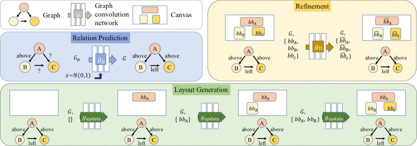
figure Graphic layout generation with user constraints. We present realistic use cases of the proposed model. Given the desired components and partial user-specified constraints among them, our model can generate layouts following these constraints. We also present example designs constructed based on the generated layouts.
1 Introduction
Graphic design surrounds us on a daily basis, from image advertisements, movie posters, and book covers to more functional presentation slides, websites, and mobile applications. Graphic design is a process of using text, images, and symbols to visually convey messages. Even for experienced graphic designers, the design process is iterative and time-consuming with many false starts and dead ends. This is further exacerbated by the proliferation of platforms and users with significantly different visual requirements and desires.
In graphic design, layout – the placement and sizing of components (e.g., title, image, logo, banner, etc.) – plays a significant role in dictating the flow of the viewer’s attention and, therefore, the order by which the information is received. Creating an effective layout requires understanding and balancing the complex and interdependent relationships amongst all of the visible components. Variations in the layout change the hierarchy and narrative of the message.
In this work, we focus on the layout generation problem that places components based on the component attributes, relationships among components, and user-specified constraints. Figure Neural Design Network: Graphic Layout Generation with Constraints illustrates examples where users specify a collection of assets and constraints, then the model would generate a design layout that satisfies all input constraints, while remaining visually appealing. Generative models have seen a success in rendering realistic natural images [7, 17, 27]. However, learning-based graphic layout generation remains less explored. Existing studies tackle layout generation based on templates [3, 12] or heuristic rules [25], and more recently using learning-based generation methods [16, 22, 33]. However, these approaches are limited in handling relationships among components. High-level concepts such as mutual relationships of components in a layout are less likely to be captured well with conventional generative models in pixel space. Moreover, the use of generative models to account for user preferences and constraints is non-trivial. Therefore, effective feature representations and learning approaches for graphic layout generation remain challenging.
In this work, we introduce neural design network (NDN), a new approach of synthesizing a graphic design layout given a set of components with user-specified attributes and constraints. We employ directional graphs as our feature representation for components and constraints since the attributes of components (node) and relations among components (edge) can be naturally encoded in a graph. NDN takes as inputs a graph constructed by desired components as well as user-specified constraints, and then outputs a layout where bounding boxes of all components are predicted. NDN consists of three modules. First, the relation prediction module takes as input a graph with partial edges, representing components and user-specified constraints, and infers a graph with complete relationships among components. Second, in the layout generation module, the model predicts bounding boxes for components in the complete graph in an iterative manner. Finally, in the refinement module, the model further fine-tunes the bounding boxes to improve the alignment and visual quality.
We evaluate the proposed method qualitatively and quantitatively on three datasets under various metrics to analyze the visual quality. The three experimental datasets are RICO [4, 24], Magazine [33], and an image banner advertisement dataset collected in this work. These datasets reasonably cover several typical applications of layout design with common components such as images, texts, buttons, toolbars and relations such as above, larger, around, etc. We construct real designs based on the generated layouts to assess the quality. We also demonstrate the efficacy of the proposed model by introducing a practical layout recommendation application.
To summarize, we make the following contributions in this work:
-
•
We propose a new approach that can generate high-quality design layouts for a set of desired components and user-specified constraints.
-
•
We validate that our method performs favorably against existing models in terms of realism, alignment, and visual quality on three datasets.
-
•
We demonstrate real use cases that construct designs from generated layouts and a layout recommendation application. Furthermore, we collect a real-world advertisement layout dataset to broaden the variety of existing layout benchmarks.
2 Related Work
Natural scene layout generation. Layout is often used as the intermediate representation in the image generation task conditioned on text [9, 11, 31] or scene graph [15]. Instead of directly learning the mapping from the source domain (e.g., text and scene graph) to the image domain, these methods model the operation as a two-stage framework. They first predict layouts conditioned on the input sources, and then generate images based on the predicted layouts. Recently, Jyothi et al. propose the LayoutVAE [16], which is a generative framework that can synthesize scene layout given a set of labels. However, a graphic design layout has several fundamental differences to a natural scene layout. The demands for relationship and alignment among components are strict in graphic design. A few pixels offsets of components can either cause a difference in visual experience or even ruin the whole design. The graphic design layout does not only need to look realistic but also needs to consider the aesthetic perspective.
Graphic design layout generation. Early work on design layout or document layout mostly relies on templates [3, 12], exemplars [21], or heuristic design rules [25, 30]. These methods rely on predefined templates and heuristic rules, for which professional knowledge is required. Therefore, they are limited in capturing complex design distributions. Other work leverages saliency maps [1] and attention mechanisms [26] to capture the visual importance of graphic designs and to trace the user’s attention. Recently, generative models are applied to graphic design layout generation [22, 33]. The LayoutGAN model [22] can generate layouts consisting of graphic elements like rectangles and triangles. However, the LayoutGAN model generates layout from input noises and fails to handle layout generation given a set of components with specified attributes, which is the common setting in graphic design. The Layout Generative Network [33] is a content-aware layout generation framework that can render layouts conditioned on attributes of components. While the goals are similar, the conventional GAN-based framework cannot explicitly model relationships among components and user-specified constraints.
Graph neural networks in vision. Graph Neural Networks (GNNs) [6, 8, 29] aim to model dependence among nodes in a graph via message passing. GNNs are useful for data that can be formulated in a graph data structure. Recently, GNNs and related models have been applied to classification [20], scene graph [2, 15, 23, 32, 34], motion modeling [13], and molecular property prediction [5, 14], to name a few. In this work, we model a design layout as a graph and apply GNNs to capture the dependency among components.
3 Graphic Layout Generation
Our goal is to generate design layouts given a set of design components with user-specified constraints. For example, in image ads creation, the designers can input the constraints such as “logo at bottom-middle of canvas”, “call-to-action button of size (100px, 500px)”, “call-to-action-button is below logo”, etc. The goal is to synthesize a set of design layouts that satisfy both the user-specified constraints as well as common rules in image ads layouts. Unlike layout templates, these layouts are dynamically created and can serve as inspirations for designers.
We introduce the neural design network using graph neural network and conditional variational auto-encoder (VAE) [19, 28] with the goal of capturing better representations of design layouts. Figure 1 illustrates the process of generating a three-component design with the proposed neural design network. In the rest of this section, we first describe the problem overview in Section 3.1. Then we detail three modules in NDN: the relation prediction (Section 3.2) and layout generation modules (Section 3.3), and refinement module (Section 3.4).
3.1 Problem Overview
The inputs to our network are a set of design components and user-specified constraints. We model the inputs as a graph, where each design component is a node and their relationships are edges. In this paper, we study two common relationships between design components: location and size.
Define , where is a set of components with each coming from a set of categories . We use to denote the canvas that is fixed in both location and size, and to denote other design components that need to be placed on the canvas, such as logo, button. and are sets of directed edges with and , where and . Here, specifies the relative size of the component, such as smaller or bigger, and can be left, right, above, below, upper-left, lower-left, etc. In addition, if anchoring on the canvas , we extend the to capture the location that is relative to the canvas, e.g., upper-left of the canvas.
Furthermore, in reality, designers often do not specify all the constraints. This results in an input graph with missing edges. Figure 1 shows an example of a three-component design with only one specified constraint “(, above, )” and several unknown relations “”. To this end, we augment and to include an additional unknown category, and represent graphs that contain unknown size or location relations as and , respectively, to indicate they are the partial graphs. In Section 3.2, we describe how to predict the unknown relations in the partial graphs.
Finally, we denote the output layout of the neural design network as a set of bounding boxes , where represents the location and shape.
In all modules, we apply the graph convolutional networks on graphs. The graph convolutional networks take as the input the features of nodes and edges, and outputs updated features. The input features can be one-hot vectors representing the categories or any embedded representations.
More implementation details can be found in the supplementary material.
3.2 Relation Prediction
In this module, we aim to infer the unknown relations in the user-specified constraints. Figure 1 shows an example where a three-component graph is given and we need to predict the missing relations between , , and . For brevity, we denote the graphs with complete relations as , and the graphs with partial relations as , which can be either or . Note that since the augmented relations include the unknown category, both and are complete graphs in practice. We also use to refer to either or depending on the context.
We model the prediction process as a paired graph-to-graph translation task: from to . Since the translation is multimodal, i.e., a graph with partial relations can be translated to many possible graphs with complete relations. Therefore, we adopt a similar framework to the multimodal image-to-image translation [35] and treat as the source domain and as the target domain. Similar to [35], the translation is a conditional generation process that maps the source graph, along with a latent code, to the target graph. The latent code is encoded from the corresponding target graph to achieve reconstruction during training, and is sampled from a prior during testing. The conditional translation encoding process is modeled as:
| (1) | ||||||
where and are graph convolutional networks, and is a relation predictor. In addition, is the set of edges in the target graph. Note that since the graph is a complete graph.
The model is trained with the reconstruction loss on the relation categories, where the indicates cross-entropy function, and a KL loss on the encoded latent vectors to facilitate sampling at inference time: , where . The objective of the relation prediction module is:
| (2) |
The reconstruction loss captures the knowledge that the predicted relations should agree with the existing relations in , and fill in any missing edge with the most likely relation discovered in the training data.
3.3 Layout Generation
Given a graph with complete relations, this module aims to generate the design layout by predicting the bounding boxes for all nodes in the graph.
Let be the graph with complete relations constructed from and , the output of the relation prediction module. We model the generation process using a graph-based iterative conditional VAE model. We first obtain the features of each component by
| (3) |
where is a graph convolutional network. These features capture the relative relations among all components. We then predict bounding boxes in an iterative manner starting from an empty canvas (i.e., all bounding boxes are unknown). As shown in Figure 1, the prediction of each bounding box is conditioned on the initial features as well as the current canvas, i.e., predicted bounding boxes from previous iterations. At iteration , the condition can be modeled as:
| (4) | ||||
where is another graph convolutional network. is a tuple of features and current canvas at iteration , and is a vector. Then we apply conditional VAE on the current bounding box conditioned on .
| (5) | ||||
where and represent encoders and decoders consisting of fully connected layers. We train the model with conventional VAE loss: a reconstruction loss and a KL loss . The objective of the layout generation module is:
| (6) |
The model is trained with teacher forcing where the ground truth bounding box at step will be used as the input for step . At test time, the model will use the actual output boxes from previous steps. In addition, the latent vector will be sampled from a conditional prior distribution , where is a prior encoder.
Bounding boxes with predefined shapes.
In many design use cases, it is often required to constrain some design components to fixed size. For example, the logo size needs to be fixed in the ad design. To achieve this goal, we augment the original layout generation module with an additional VAE encoder to ensure the encoded latent vectors can be decoded to bounding boxes with desired widths and heights. Similar to (5), given a ground-truth bounding box , we obtain the reconstructed bounding box with and . Then, instead of applying reconstruction loss on whole bounding boxes tuples, we only enforce the reconstruction of width and height with
| (7) |
The objective of the augmented layout generation module is given by:
| (8) |
3.4 Layout Refinement
We predict bounding boxes in an iterative manner that requires to fix the predicted bounding boxes from the previous iteration. As a result, the overall bounding boxes might not be optimal, as shown in the layout generation module in Figure 1. To tackle this issue, we fine-tune the bounding boxes for better alignment and visual quality in the final layout refinement module. Given a graph with ground-truth bounding boxes , we simulate the misalignment by randomly apply offsets on , where is the uniform distribution. We obtain misaligned bounding boxes = . We apply a graph convolutional network for finetuning:
| (9) |
The model is trained with reconstruction loss .
4 Experiments and Analysis
Datasets
We perform the evaluation on three datasets:
-
•
Magazine [33]. The dataset contains images of magazine pages and categories (texts, images, headlines, over-image texts, over-image headlines, backgrounds).
-
•
RICO [4, 24]. The original dataset contains images of the Android apps interface and categories. We choose most frequent categories (toolbars, images, texts, icons, buttons, inputs, list items, advertisements, pager indicators, web views, background images, drawers, modals) and filter the number of components within an image to be less than , totaling images.
-
•
Image banner ads. We collect image banner ads of the size via image search using keywords such as “car ads”. We annotate bounding boxes of categories: images, regions of interest, logos, brand names, texts, and buttons.
Evaluated methods.
We evaluate and compare the following algorithms:
-
•
sg2im [15]. The model is proposed to generate a natural scene layout from a given scene graph. The sg2im method takes as inputs graphs with complete relations in the setting where all constraints are provided. When we compare with this method in the setting where no constraint is given, we simplify the input scene graph by removing all relations. We refer the simplified model as sg2im-none.
-
•
LayoutVAE [16]. This model takes a label set as input, and predicts the number of components for each label as well as the locations of each component. We compare with the second stage of the LayoutVAE model (i.e., the bounding box prediction stage) by giving the number of components for each label. In addition, we refer to LayoutVAE-loo as the model that predicts the bounding box of a single component when all other components are provided and fixed (the leave-one-out setting).
-
•
Neural Design Network. We refer to NDN-none when the input contains no prior constraint, NDN-all in the same setting as sg2im when all constraints are provided, and NDN-loo in the same setting as LayoutVAE-loo.
We do not compare our method with LayoutGAN [22] since LayoutGAN generates outputs in an unconditional manner (i.e., generation from sampled noise vectors). Even in the no-constraint setting, it is difficult to conduct fair comparisons as multiple times of resampling are required to generate the same combinations of components.
4.1 Implementation Details
In this work, , , and consists of fully-connected layers. In addition, , , , and consist of graph convolution layers. The dimension of latent vectors in the relation prediction and layout generation module is . The input features of nodes and edges are obtained from a dictionary mapping, which is trained along with the model. For training, we use the Adam optimizer [18] with batch size of , learning rate of , and . In all experiments, we set the hyper-parameters as follows: , , , and . We use a predefined order of component sets in all experiments.
For the relation prediction module, the graphs with partial constraint are generated from the ground-truth graph with dropout rate. For the layout generation module, the input graphs with complete relations are constructed from the ground-truth layouts. The location and size relations are obtained by ground-truth bounding boxes. The corresponding outputs are the bounding boxes from the ground-truth layouts.
Since the location relations are discretized and mutually exclusive, there might be some ambiguity. For example, a component is both “above” and “right” of another component when it is in the upper-right direction to the other. To handle the ambiguity, we predefine the order when conflicts occur. Specifically, “above” and “below” have higher priority than “left of” and “right of”.
More implementation details can be found in the supplementary material.
| Datasets | Ads | Magazine | RICO | |||
| FID | Align. | FID | Align. | FID | Align. | |
| sg2im-none | 116.63 | 0.63 | 95.81 | 0.97 | 269.60 | 0.14 |
| LayoutVAE | 138.11 | 1.210.08 | 81.5636.78 | .3140.11 | 192.1129.97 | 1.190.39 |
| NDN-none | 129.6832.12 | 0.910.07 | 69.4332.92 | 2.510.09 | 143.5122.36 | 0.910.03 |
| sg2im | 230.44 | 0.0069 | 102.35 | 0.0178 | 190.68 | 0.007 |
| NDN-all | 168.4421.83 | 0.610.05 | 82.7716.24 | 1.510.09 | 64.7811.60 | 0.320.02 |
| Pred. error | Align. | Pred. error | Align. | Pred. error | Align. | |
| LayoutVAE-loo | 0.0710.002 | 0.480.01 | 0.0590.002 | 1.410.02 | 0.0450.0021 | 0.390.02 |
| NDN-loo | 0.0430.001 | 0.360.01 | 0.0240.0002 | 1.300.01 | 0.0180.002 | 0.140.01 |
| real data | - | 0.0034 | - | 0.0126 | - | 0.0012 |
4.2 Quantitative Evaluation
Realism and accuracy. We evaluate the visual quality following Fréchet Inception Distance (FID) [10] by measuring how close the distribution of generated layout is to the real ones. We train a binary layout classifier to discriminate between good and bad layouts. The bad layouts are generated by randomly moving component locations of good layouts. The classifier consists of four graph convolution layers and three fully connected layers. The binary classifier achieves classification accuracy of , , and on the Ads, Magazine, and RICO datasets, respectively. We extract the features of the second from the last fully connected layer to measure FID.
We measure FID in two settings. First, a model predicts bounding boxes without any constraints. That is, only the number and the category of components are provided. We compare with LayoutVAE and sg2im-none in this setting. Second, a model predicts bounding boxes with all constraints provided. We compare with sg2im in this setting since LayoutVAE cannot take constraints as inputs. The first two rows in Table 1 present the results of these two settings. Since LayoutVAE and the proposed method are both stochastic models, we generate 100 samples for each testing design in each trial. The results are averaged over trials. In both no-constraint and all-constraint settings, the proposed method performs favorably against the other schemes.
We also measure the prediction accuracy in the leave-one-out setting, i.e., predicting the bounding box of a component when bounding boxes of other components are provided. We measure the accuracy by the error between the predicted and the ground-truth bounding boxes. The third row of Table 1 shows the comparison to the LayoutVAE-loo method in this setting. The proposed method gains better accuracy with statistical significance ( 95%), indicating that the graph-based framework encodes better relations among components.
|
|
|
|
Refinement | FID | Align. | ||||||||
| 0 | 0 | 0 | 0 | ✓ | 143.5122.36 | 0.910.03 | ||||||||
| 20 | 20 | 0 | 0 | ✓ | 141.6420.01 | 0.870.03 | ||||||||
| 0 | 0 | 20 | 20 | ✓ | 129.9223.76 | 0.810.03 | ||||||||
| 20 | 20 | 20 | 20 | 126.1823.11 | 0.740.02 | |||||||||
| 20 | 20 | 20 | 20 | ✓ | 125.4121.68 | 0.700.02 | ||||||||
| 100 | 100 | 100 | 100 | 70.5512.68 | 0.360.02 | |||||||||
| 100 | 100 | 100 | 100 | ✓ | 64.7811.60 | 0.320.02 |
| Order | Size | Occurence | Random | ||
| FID | 132.84 | 136.22 | 143.51 | ||
|
1.080.04 | 1.020.04 | 0.910.03 |
| Dataset | Ads | Magazine | RICO | ||
|
96.8 | 95.9 | 98.2 |
Alignment. Alignment is an important principle in design creation. In most good designs, components need to be either in center alignment or edge alignment (e.g., left- or right-aligned). Therefore, in addition to realism, we explicitly measure the alignment among components using:
| (10) |
where is the number of generated layouts, is the component of the layout. In addition, , , and are alignment functions where the distances between the left, center, and right of components are measured, respectively.
Table 1 presents the results in the no-constraint, all-constraint, and leave-one-out settings. The results are also averaged over trials. The proposed method performs favorably against other methods. The sg2im-none method gets better alignment score since it tends to predict bounding boxes in several fixed locations when no prior constraint is provided, which leads to worse FID. For similar reasons, the sg2im method gains a slightly higher alignment score on RICO.
Partial constraints. Previous experiments are conducted under the settings of either no constraints or all constraints provided. Now, we demonstrate the efficacy of the proposed method on handling partial constraints. Table 2 shows the results of layout prediction with different percentages of prior constraints provided. We evaluate the partial constraints setting using the RICO dataset, which is the most difficult dataset in terms of diversity and complexity. Ideally, the FID and alignment scores should be similar regardless of the percentage of constraints given. However, in the challenging RICO dataset, the prior information of size and location still greatly improves the visual quality, as shown in Table 2, The location constraints contribute to more improvement since they explicitly provide guidance from the ground-truth layouts. As for the alignment score, layouts in all settings perform similarly. Furthermore, the refinement module can slightly improve the alignment score as well as FID.
User constraint consistency The major goal of the proposed model is to generate layouts according to user-specified constraints. Therefore, we explicitly measure the consistency between the relations among generated components and the original user-specified constraints. Table 4 shows that the generated layouts reasonably conform to the input constraints.
Order of components. Since the proposed model predicts layouts in an iterative manner, the order of the components plays an important role. We evaluate our method using three different strategies of defining orders: ordered by size, ordered by occurrences, and random order. We show the comparisons in Table 4. We have a similar finding as in LayoutVAE that the order of components affects the generation results. However, we use the random order in all our experiments since our goal is not only to generate layouts, but also enable flexible user control. In user cases such as leave-one-out prediction and layout recommendation, using random order can better align the training and testing scenarios.
4.3 Qualitative Evaluation
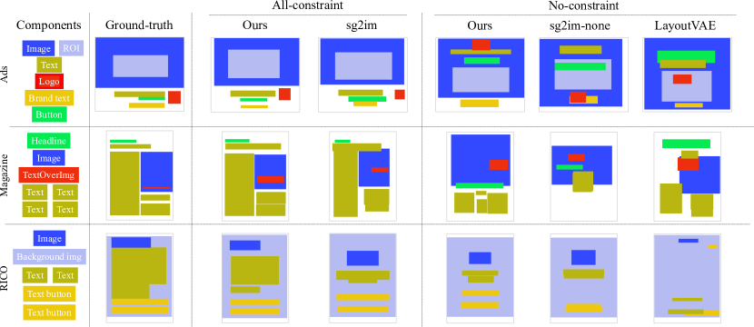
We compare the proposed method with related work in Figure 2. In the all-constraint setting, both the sg2im method and the proposed model can generate reasonable layouts similar to the ground-truth layouts. However, the proposed model can better tackle alignment and overlapping issues. In the no-constraint setting, the sg2im-none method tends to place components of the same categories at the same location, like the “text”s in the second row and the “text”s and “text button”s in the third row. The LayoutVAE method, on the other hand, cannot handle relations among components well without using graphs. The proposed method can generate layouts with good visual quality, even with no constraint provided.
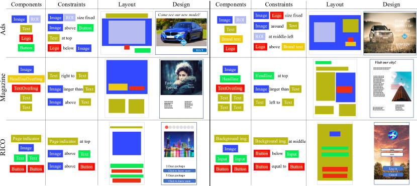
Partial constraints. In Figure 3, we present the results of layout generation given several randomly selected constraints on size and location. Our model generates design layouts that are both realistic and follows user-specified constraints. To better visualize the quality of the generated layouts, we present designs with real assets generated from the predicted layouts. Furthermore, we can constrain the size of specific components to desired shapes (e.g., we fix the image and logo size in the first row of Figure 3.) using the augmented layout generation module.
![[Uncaptioned image]](/html/1912.09421/assets/x5.png) \captionof
\captionof
figureLayout Recommendation. We show examples of layout recommendations where locations of desired components are recommended given the current layouts.
![[Uncaptioned image]](/html/1912.09421/assets/x6.png) \captionof
\captionof
figureFailure cases. Generation may fail when the sampled latent vectors locate in under-sample spaces or the characteristics of inputs differ greatly from that in the training data.
Layout recommendation. The proposed model can also help designers decide the best locations of a specific design component (e.g., logo, button, or headline) when a partial design layout is provided. This can be done by building graphs with partial location and size relations based on the current canvas and set the relations to target components as unknown. We then complete this graph using the relation prediction module. Finally, conditioned on the predicted graph as well as current canvas, we perform iterative bounding boxes prediction with the layout generation module. Figure 4.3 shows examples of layout recommendations.
Failure cases. Several reasons may lead to undesirable generation. First, due to the limited amount of training data, the sampled latent vectors used for generation might locate in undersampled spaces that are not fully exploited during training. Second, the characteristic of the set of components is too different from the training data. For example, the lower-left image in Figure 4.3 demonstrates a generation requiring three buttons and two logos, which are less likely to exist in real designs.
5 Conclusion and Future Work
In this work, we propose a neural design network to handle design layout generation given user-specified constraints. The proposed method can generate layouts that are visually appealing and follow the constraints with a three-module framework, including a relation prediction module, a layout generation module, and a refinement module. Extensive quantitative and qualitative experiments demonstrate the efficacy of the proposed model. We also present examples of constructing real designs based on generated layouts, and an application of layout recommendation.
Visual design creation is an impactful but understudied topic in our community. It is extremely challenging. Our work is among one of the first works tackling graphic design in a well-defined setting that is reasonably close to the real use case. However, graphic design is a complicated process involving content attributes such as color, font, semantic labels, etc. Future directions may include content-aware graphic design or fine-grained layout generation beyond the bounding box.
6 Acknowledgement
This work is supported in part by the NSF CAREER Grant .
References
- [1] Bylinskii, Z., Kim, N.W., O’Donovan, P., Alsheikh, S., Madan, S., Pfister, H., Durand, F., Russell, B., Hertzmann, A.: Learning visual importance for graphic designs and data visualizations. In: UIST (2017)
- [2] Cheng, Y.C., Lee, H.Y., Sun, M., Yang, M.H.: Controllable image synthesis via segvae. In: ECCV (2020)
- [3] Damera-Venkata, N., Bento, J., O’Brien-Strain, E.: Probabilistic document model for automated document composition. In: DocEng (2011)
- [4] Deka, B., Huang, Z., Franzen, C., Hibschman, J., Afergan, D., Li, Y., Nichols, J., Kumar, R.: Rico: A mobile app dataset for building data-driven design applications. In: UIST (2017)
- [5] Duvenaud, D.K., Maclaurin, D., Iparraguirre, J., Bombarell, R., Hirzel, T., Aspuru-Guzik, A., Adams, R.P.: Convolutional networks on graphs for learning molecular fingerprints. In: NeurIPS (2015)
- [6] Goller, C., Kuchler, A.: Learning task-dependent distributed representations by backpropagation through structure. In: ICNN (1996)
- [7] Goodfellow, I., Pouget-Abadie, J., Mirza, M., Xu, B., Warde-Farley, D., Ozair, S., Courville, A., Bengio, Y.: Generative adversarial nets. In: NeurIPS (2014)
- [8] Gori, M., Monfardini, G., Scarselli, F.: A new model for learning in graph domains. In: IJCNN (2005)
- [9] Gupta, T., Schwenk, D., Farhadi, A., Hoiem, D., Kembhavi, A.: Imagine this! scripts to compositions to videos. In: ECCV (2018)
- [10] Heusel, M., Ramsauer, H., Unterthiner, T., Nessler, B., Hochreiter, S.: GANs trained by a two time-scale update rule converge to a local nash equilibrium. In: NeurIPS (2017)
- [11] Hong, S., Yang, D., Choi, J., Lee, H.: Inferring semantic layout for hierarchical text-to-image synthesis. In: CVPR (2018)
- [12] Hurst, N., Li, W., Marriott, K.: Review of automatic document formatting. In: DocEng (2009)
- [13] Jain, A., Zamir, A.R., Savarese, S., Saxena, A.: Structural-rnn: Deep learning on spatio-temporal graphs. In: CVPR (2016)
- [14] Jin, W., Yang, K., Barzilay, R., Jaakkola, T.: Learning multimodal graph-to-graph translation for molecular optimization. In: ICLR (2019)
- [15] Johnson, J., Gupta, A., Fei-Fei, L.: Image generation from scene graphs. In: CVPR (2018)
- [16] Jyothi, A.A., Durand, T., He, J., Sigal, L., Mori, G.: Layoutvae: Stochastic scene layout generation from a label set. In: ICCV (2019)
- [17] Karras, T., Laine, S., Aila, T.: A style-based generator architecture for generative adversarial networks. In: CVPR (2019)
- [18] Kingma, D., Ba, J.: Adam: A method for stochastic optimization. In: ICLR (2015)
- [19] Kingma, D.P., Welling, M.: Auto-encoding variational bayes. In: ICLR (2014)
- [20] Kipf, T.N., Welling, M.: Semi-supervised classification with graph convolutional networks. In: ICLR (2017)
- [21] Kumar, R., Talton, J.O., Ahmad, S., Klemmer, S.R.: Bricolage: example-based retargeting for web design. In: SIGCHI (2011)
- [22] Li, J., Yang, J., Hertzmann, A., Zhang, J., Xu, T.: Layoutgan: Generating graphic layouts with wireframe discriminators. In: ICLR (2019)
- [23] Li, Y., Jiang, L., Yang, M.H.: Controllable and progressive image extrapolation. arXiv preprint arXiv:1912.11711 (2019)
- [24] Liu, T.F., Craft, M., Situ, J., Yumer, E., Mech, R., Kumar, R.: Learning design semantics for mobile apps. In: UIST (2018)
- [25] O’Donovan, P., Agarwala, A., Hertzmann, A.: Learning layouts for single-pagegraphic designs. TVCG (2014)
- [26] Pang, X., Cao, Y., Lau, R.W., Chan, A.B.: Directing user attention via visual flow on web designs. ACM TOG (Proc. SIGGRAPH) (2016)
- [27] Razavi, A., Oord, A.v.d., Vinyals, O.: Generating diverse high-fidelity images with vq-vae-2. arXiv preprint arXiv:1906.00446 (2019)
- [28] Rezende, D.J., Mohamed, S., Wierstra, D.: Stochastic backpropagation and approximate inference in deep generative models. In: ICML (2014)
- [29] Scarselli, F., Gori, M., Tsoi, A.C., Hagenbuchner, M., Monfardini, G.: The graph neural network model. TNN (2008)
- [30] Tabata, S., Yoshihara, H., Maeda, H., Yokoyama, K.: Automatic layout generation for graphical design magazines. In: SIGGRAPH (2019)
- [31] Tan, F., Feng, S., Ordonez, V.: Text2scene: Generating abstract scenes from textual descriptions. In: CVPR (2019)
- [32] Tseng, H.Y., Lee, H.Y., Jiang, L., Yang, W., Yang, M.H.: Retrievegan: Image synthesis via differentiable patch retrieval. In: ECCV (2020)
- [33] Xinru Zheng, Xiaotian Qiao, Y.C., Lau, R.W.: Content-aware generative modeling of graphic design layouts. SIGGRAPH (2019)
- [34] Yang, J., Lu, J., Lee, S., Batra, D., Parikh, D.: Graph r-cnn for scene graph generation. In: ECCV (2018)
- [35] Zhu, J.Y., Zhang, R., Pathak, D., Darrell, T., Efros, A.A., Wang, O., Shechtman, E.: Toward multimodal image-to-image translation. In: NeurIPS (2017)