Gravitomagnetism in the Lewis cylindrical metrics

Abstract

The Lewis solutions describe the exterior gravitational field produced by infinitely long rotating cylinders, and are useful models for global gravitational effects. When the metric parameters are real (Weyl class), the exterior metrics of rotating and static cylinders are locally indistinguishable, but known to globally differ. The significance of this difference, both in terms of physical effects (gravitomagnetism) and of the mathematical invariants that detect the rotation, remain open problems in the literature. In this work we show that, by a rigid coordinate rotation, the Weyl class metric can be put into a “canonical” form where the Killing vector field $\partial_{t}$ is time-like everywhere, and which depends explicitly only on three parameters with a clear physical significance: the Komar mass and angular momentum per unit length, plus the angle deficit. This new form of the metric reveals that the two settings differ only at the level of the gravitomagnetic vector potential which, for a rotating cylinder, cannot be eliminated by any global coordinate transformation. It manifests itself in the Sagnac and gravitomagnetic clock effects. The situation is seen to mirror the electromagnetic field of a rotating charged cylinder, which likewise differs from the static case only in the vector potential, responsible for the Aharonov-Bohm effect, formally analogous to the Sagnac effect. The geometrical distinction between the two solutions is also discussed, and the notions of local and global staticity revisited. The matching in canonical form to the van Stockum interior cylinder is also addressed.

, ,

Keywords: gravitomagnetism, Sagnac effect, frame-dragging, van Stockum cylinder, gravito-electromagnetic analogy, 1 + 3 quasi-Maxwell formalism, locally and globally static spacetimes

1 Introduction

The Lewis metrics [1] are the general stationary solution of the vacuum Einstein field equations with cylindrical symmetry, and are usually interpreted as describing the exterior gravitational field produced by infinitely long rotating cylinders (for a recent review on cylindrical systems in General Relativity, see [2]). They are divided into two sub-classes: the Lewis class and the Weyl class, the latter corresponding to the case where all the metric parameters are real. The Weyl class metrics have the same Cartan scalars as in the special case of a static cylinder (Levi-Civita metric), and so are locally indistinguishable [3]; they are known, however, to have distinct global properties, namely in the matching to the interior solutions (as the former, but not the latter, can be matched to rotating interior cylinders). The physical implications of such difference remain an unanswered question in the literature [3, 4, 5]; they are expected to be manifested as “gravitomagnetism”, the gravitational effects generated by the motion of matter (thus known due to their many analogies with magnetism). From a mathematical point of view, this distinction also remains an open question, namely whether it stems from topology [3, 4] or geometry [6], what are the invariants that detect the rotation, or what is the nature of the “transformation” [3, 7, 8] that is known to relate the Weyl class rotating and static metrics. The physical significance of the four Lewis parameters also remains unclear [5]; it has been shown in [4] that only three are independent, but an explicit form of the metric in terms of three parameters, with a clear physical interpretation, has proved elusive. Another open question is the rather mysterious “force” parallel to the cylinder’s axis found in the literature [9], which seemingly deflects test particles moving in these spacetimes axially. In this work we address these questions.

This paper is organized as follows. In the preliminary Section 2, after briefly reviewing some relevant features of stationary spacetimes, we discuss and formulate, in a suitable framework, the Sagnac effect, which plays a crucial role in the context of this work. In Sec. 3 we discuss, in parallel with their electromagnetic analogues, the different levels of gravitomagnetism, corresponding to different levels of differentiation of the “gravitomagnetic vector potential”; special attention is given to the gravitomagnetic clock effect — another important effect in this work — which is revisited and reinterpreted in the framework herein. In Sec. 4, as a preparation for the gravitational problem, we study the electromagnetic field produced by infinitely long rotating charged cylinders, as viewed from both static and rotating frames, and the Aharonov-Bohm effect. In Sec. 5 we start by discussing the Lewis metrics of the Weyl class in their usual form given in the literature, studying the inertial and tidal fields as measured in the associated reference frame; we also dissect (Sec. 5.1.2) the origin of the axial coordinate acceleration found in the literature. Subsections 5.2 and 5.3 contain the main results in this paper. In 5.2 we show that the usual form of the Weyl class metrics is actually written in a system of rigidly rotating coordinates; gauging such rotation away leads to a coordinate system which is inertial at infinity (thus fixed with respect to the “distant stars”), the Killing vector field $\partial_{t}$ is time-like everywhere, and the metric depends explicitly only on three parameters: the Komar mass and angular momentum per unit length, plus the angle deficit. We dub such form of the metric “canonical”. It makes transparent that the gravitational fields of (Weyl class) rotating and static cylinders differ only in the gravitomagnetic potential 1-form $\bm{\mathcal{A}}$ (which is non-vanishing in the former); the observers at rest measure the same inertial and tidal fields (Sec. 5.2.3), the only distinction being the global effects governed by $\bm{\mathcal{A}}$. The situation is seen to exactly mirror the electromagnetic fields of rotating/static charged cylinders. In Sec. 5.3 this distinction is explored both on physical grounds, putting forth (thought) physical apparatuses to reveal it (Sec. 5.3.1), and on geometrical grounds (Sec. 5.3.4). It turns out to be an archetype of the contrast between globally static, and locally but non-globally static spacetimes; hence we also revisit (Secs. 5.3.2-5.3.3) the notions of local and global staticity in the literature, devising equivalent formulations that are more enlightening in this context. In Sec. 5.4 we discuss the matching to the interior van Stockum cylinder. We first establish the correspondence between the Lewis and van Stockum exterior solutions, and, using their usual forms in the literature, obtain the matching to the interior van Stockum solution, using the so-called “quasi-Maxwell” formalism. Then, in the same framework, we obtain the matching in canonical form. Finally, in Sec. 5.5, we briefly discuss the Lewis metrics of the Lewis class, pointing out their fundamental differences from the Weyl class in the framework herein.

1.1 Notation and conventions

We use the signature $(-+++)$; $\epsilon_{\alpha\beta\gamma\delta}\equiv\sqrt{-g}[\alpha\beta\gamma\delta]$ is the 4-D Levi-Civita tensor, with the orientation $[1230]=1$ (i.e., in flat spacetime, $\epsilon_{1230}=1$); Greek letters $\alpha$, $\beta$, $\gamma$, … denote 4D spacetime indices, running 0-3; Roman letters $i,j,k,...$ denote spatial indices, running 1-3. Our convention for the Riemann tensor is $R_{\ \beta\mu\nu}^{\alpha}=\Gamma_{\beta\nu,\mu}^{\alpha}-\Gamma_{\beta\mu,\nu}^{\alpha}+...$ . $\star$ denotes the Hodge dual (e.g. $\star F_{\alpha\beta}\equiv\epsilon_{\alpha\beta}^{\ \ \ \mu\nu}F_{\mu\nu}/2$, for a 2-form $F_{\alpha\beta}=F_{[\alpha\beta]}$). The basis vector corresponding to a coordinate $\phi$ is denoted by $\partial_{\phi}$, and its $\alpha$-component by $\partial_{\phi}^{\alpha}\equiv\delta_{\phi}^{\alpha}$.

2 Preliminaries

The line element $ds^{2}=g_{\alpha\beta}dx^{\alpha}dx^{\beta}$ of a stationary spacetime can generically be written as

$$ds^{2}=-e^{2\Phi}(dt-\mathcal{A}_{i}dx^{i})^{2}+h_{ij}dx^{i}dx^{j}\ ,$$ (1)

where $e^{2\Phi}=-g_{00}$, $\Phi\equiv\Phi(x^{j})$, $\mathcal{A}_{i}\equiv\mathcal{A}_{i}(x^{j})=-g_{0i}/g_{00}$, and $h_{ij}\equiv h_{ij}(x^{k})=g_{ij}+e^{2\Phi}\mathcal{A}_{i}\mathcal{A}_{j}$. Observers whose worldlines are tangent to the timelike Killing vector field $\partial_{t}$ are at rest in the coordinate system of (1); they are sometimes called “static” or “laboratory” observers. Their 4-velocity is

$$u^{\alpha}\equiv u_{{\rm lab}}^{\alpha}=(-g_{00})^{-1/2}\partial_{t}^{\alpha}=e^{-\Phi}\partial_{t}^{\alpha}\equiv e^{-\Phi}\delta_{0}^{\alpha}\ .$$ (2)

The quotient of the spacetime by the worldlines of the laboratory observers yields a 3-D manifold $\Sigma$ in which $h_{ij}$ is a Riemannian metric, called the spatial or “orthogonal” metric [10, 11, 12, 13, 14, 15]. It can be identified in spacetime with the projector orthogonal to $u^{\alpha}$ (space projector with respect to $u^{\alpha}$),

$$h_{\alpha\beta}\equiv u_{\alpha}u_{\beta}+g_{\alpha\beta}\ ,$$ (3)

and yields the spatial distances between neighboring laboratory observers, as measured through Einstein’s light signaling procedure [10]. In this work we will deal with axistationary spacetimes, whose line element simplifies to

$$ds^{2}=-e^{2\Phi}(dt-\mathcal{A}_{\phi}d\phi)^{2}+h_{ij}dx^{i}dx^{j}\ .$$ (4)

2.1 Stationary observers, angular momentum, and ZAMOs

Stationary spacetimes admit a privileged class of observers who see an unchanging spacetime geometry in their neighborhood, dubbed “stationary observers” [16, 17]. Each of their worldlines is tangent to a time-like Killing vector, forming congruences tangent to so-called “quasi-Killing vector fields” [18] $\chi^{\beta}=\partial_{t}^{\beta}+\sum_{n}\alpha_{n}\xi_{(n)}^{\beta}$, where the $\xi_{(n)}^{\beta}$ are spacelike Killing vectors, and the coefficients $\alpha_{n}$ are such that $\mathcal{L}_{\chi}\alpha_{n}=0$. Two classes of stationary observers are especially important in this work. One are the rest or “laboratory” observers, defined in (2). In spite of being at rest, their angular momentum is, in general, non-zero. Take the spacetime to be axisymmetric as in (4), and consider a test particle of 4-momentum $P^{\alpha}=mu^{\alpha}$ and rest mass $m$; the component of its angular momentum along the symmetry axis is given by [16, 17] $P_{\phi}=mu_{\phi}$. Hence, the laboratory observers have an angular momentum per unit mass

$$u_{\phi}=u^{0}g_{0\phi}=\frac{g_{0\phi}}{\sqrt{-g_{00}}}=e^{\Phi}\mathcal{A}_{\phi}\ ,$$ (5)

which is zero iff $g_{0\phi}=0$. Another important class of stationary observers in axistationary spacetimes are those in circular motion for which the angular momentum (i.e., $P_{\phi}$) vanishes — the zero angular momentum observers (ZAMOs). Their 4-velocity, $u_{{\rm ZAMO}}^{\alpha}=u_{{\rm ZAMO}}^{0}\partial_{0}^{\alpha}+u_{{\rm ZAMO}}^{\phi}\partial_{\phi}^{\alpha}$, is such that $(u_{{\rm ZAMO}})_{\phi}=0$, i.e., they have angular velocity

$$\Omega_{{\rm ZAMO}}\equiv\frac{u_{{\rm ZAMO}}^{\phi}}{u_{{\rm ZAMO}}^{0}}=-\frac{g_{0\phi}}{g_{\phi\phi}}\ .$$ (6)

Thus, $\Omega_{{\rm ZAMO}}=0$ iff $g_{0\phi}=0$.

2.2 Sagnac effect

A key effect in the context of this work is the Sagnac effect [19, 20, 21, 22, 23, 24, 25, 26, 27]. It consists of the difference in arrival times of light-beams propagating around a closed path in opposite directions. It is a measure of the absolute rotation of an apparatus, i.e., its rotation relative to the “spacetime geometry” [16]. It was originally introduced in the context of flat spacetime [19, 20, 21, 22, 24], where the time difference is originated by the rotation of the apparatus with respect to global inertial frames; but, in the presence of a gravitational field, it arises also in apparatuses which are fixed relative to the distant stars (i.e., to asymptotic inertial frames); the effect is in this case assigned to “frame-dragging”.

In stationary conditions, both effects can be read from the spacetime metric (1), which encompasses the flat Minkowski metric expressed in a rotating coordinate system, as well as arbitrary stationary gravitational fields. Along a photon worldline, $ds^{2}=0$; by (1), this yields the two solutions $dt=\mathcal{A}_{i}dx^{i}\pm e^{-\Phi}\sqrt{h_{ij}dx^{i}dx^{j}}$. We are interested in future-oriented worldlines, defined by $k_{\alpha}\partial_{t}^{\alpha}=k_{0}<0$, where $k^{\alpha}\equiv dx^{\alpha}/d\lambda$ is the vector tangent to the photon’s worldline. Since $k_{0}<0\Leftrightarrow dt>\mathcal{A}_{i}dx^{i}$, such worldlines correspond to the $+$ solution for $dt$:

$$dt=\mathcal{A}_{i}dx^{i}+e^{-\Phi}\sqrt{h_{ij}dx^{i}dx^{j}}\equiv\mathcal{A}_{i}dx^{i}+e^{-\Phi}dl\ ,$$

where $dl\equiv\sqrt{h_{ij}dx^{i}dx^{j}}$ is the spatial distance element. Consider photons constrained to move within a closed loop $C$ in the space manifold $\Sigma$ (that is, the photons’ worldlines are such that their projection on the space manifold $\Sigma$ yields a closed path $C$, see Fig. 2 of [25]); for instance, within an optical fiber loop. Using the + (-) sign to denote the anti-clockwise (clockwise) directions, the coordinate time it takes for a full loop is, respectively,

$$t_{\pm}=\oint_{\pm C}dt=\oint_{C}e^{-\Phi}dl\pm\oint_{C}\mathcal{A}_{i}dx^{i}\ .$$

Therefore, the Sagnac coordinate time delay $\Delta t$ is

$$\Delta t\equiv t_{+}-t_{-}=2\oint_{C}\mathcal{A}_{i}dx^{i}=2\oint_{C}\bm{\mathcal{A}}\ ,$$ (7)

where in the last equality we identified (see e.g. [16]) $\mathcal{A}_{i}dx^{i}$ with the 1-form $\bm{\mathcal{A}}\equiv\mathcal{A}_{i}\mathbf{d}x^{i}$, where $\mathbf{d}x^{i}$ are basis 1-forms both on the spacetime manifold and also on the space manifold $\Sigma$ (since $\{x^{i}\}$ is a coordinate chart on the latter). In Eq. (7) $\bm{\mathcal{A}}$ is, as usual, understood as its restriction to the curve $C$, $\bm{\mathcal{A}}|_{C}$. In what follows it will also be useful to write this result in a different form. Consider a 2-D submanifold $\mathcal{S}$ on $\Sigma$ with boundary $\partial\mathcal{S}\equiv C$. Then, by the generalized Stokes theorem,

$$\Delta t=2\oint_{\partial\mathcal{S}}\bm{\mathcal{A}}=2\int_{\mathcal{S}}\mathbf{d}\bm{\mathcal{A}}=2\int_{\mathcal{S}}(\partial\times\bm{\mathcal{A}})^{k}d\mathcal{S}_{k}\ ,$$ (8)

where $\mathbf{d}\bm{\mathcal{A}}=\mathcal{A}_{j,i}\mathbf{d}x^{i}\wedge\mathbf{d}x^{j}=\mathcal{A}_{[j,i]}\mathbf{d}x^{i}\wedge\mathbf{d}x^{j}$ is the exterior derivative of $\bm{\mathcal{A}}$, and its restriction to $\mathcal{S}$ is assumed above; $(\partial\times\bm{\mathcal{A}})^{k}\equiv\epsilon^{ijk}\mathcal{A}_{j,i}$ is the vector dual to $\mathcal{A}_{[j,i]}=\epsilon_{ijk}(\partial\times\bm{\mathcal{A}})^{k}/2$, and $d\mathcal{S}_{k}\equiv\epsilon_{ijk}\mathbf{d}x^{i}\wedge\mathbf{d}x^{j}/2$ is an area element of $\mathcal{S}$ (volume form of $\mathcal{S}$ [16]). The latter two quantities rely on endowing the space manifold $\Sigma$ with some metric $(g_{\Sigma})_{ij}$ (even though the integrand is metric independent), with $\epsilon_{ijk}=\sqrt{g_{\Sigma}}[ijk]$ the corresponding Levi-Civita tensor.

The proper time of the laboratory observers (2) is related to the coordinate time by $dt/d\tau=u^{0}=(-g_{00})^{-1/2}$; hence, the Sagnac time delay as measured by the local laboratory observer is

$$\Delta\tau = \sqrt{-g_{00}}\Delta t=e^{\Phi}\Delta t\ .$$ (9)

2.2.1 Axistationary case, circular loop around the axis

Consider an axistationary metric (4), and a circular optical fiber loop centered at the symmetry axis, as depicted in Fig. 1. From Eq. (7), counter-propagating light beams complete such loop with a coordinate time difference,

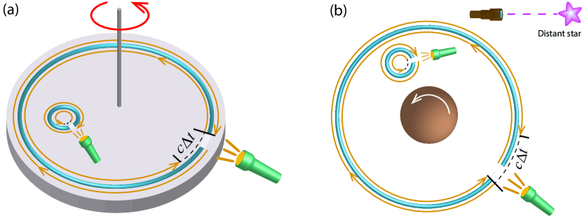
Figure 1: (a) Sagnac effect in special relativity: a flashlight sends light beams propagating in opposite directions along optical fiber loops attached to a rotating platform; they take different times to complete the loop, the co-rotating beam taking longer. (b) General relativistic Sagnac effect (“frame dragging”): optical fiber loops fixed with respect to the “distant stars” (i.e., to the asymptotic inertial frame at infinity), placed around, or in the vicinity, of a spinning object. Again, counter-propagating light beams take different times to complete the loops. In both (a) and (b) the coordinate time difference $\Delta t$ of arrival is twice the circulation of the gravitomagnetic potential 1-form $\bm{\mathcal{A}}$ [cf. Eq. (7)]; that amounts to the component $\mathcal{A}_{\phi}$ governing the effect for the circular loops around the axis, and (approximately) its curl $\partial\times\bm{\mathcal{A}}$ (times the enclosed area) for the small loops (optical gyroscopes).

$$\Delta t=2\oint_{C}\mathcal{A}_{\phi}d\phi=2\mathcal{A}_{\phi}\int_{0}^{2\pi}d\phi=4\pi\mathcal{A}_{\phi}\ .$$ (10)

In terms of the proper time of the local laboratory observer (2), the difference is $\Delta\tau=\sqrt{-g_{00}}\Delta t=4\pi u_{\phi}$. That is, it is, up to a $4\pi$ factor, the angular momentum per unit mass of the apparatus (or, equivalently, of the laboratory observers attached to it), cf. Sec. 2.1. Hence, in such an apparatus, a Sagnac effect arises iff its angular momentum is non-zero. Notice that this singles out the zero angular momentum observers (ZAMOs) as those which regard the $\pm\phi$ directions as geometrically equivalent; for this reason they are said to be those that do not rotate with respect to “the local spacetime geometry” [16].

Physical interpretation.— In the flat spacetime case in Fig. 1 (a), the physical interpretation of the Sagnac effect is simple, from the point of view of an inertial frame: the beams undergo different paths in their round trips. The co-rotating one undergoes a longer path, comparing to the case that the apparatus does not rotate, because the arrival point is “running away” from the beam during the trip, thus taking longer to complete the loop (since the speed of light is the same). Conversely, the counter-rotating one undergoes a shorter path, since the arrival point is approaching the beam during the trip. This provides an intuitive argument for understanding the general relativistic Sagnac effect as well. Consider the gravitational field of a spinning body, as depicted in Fig. 1(b). As is well known, in such a field the observers (or objects) with zero angular momentum actually have, from the point of view of a star-fixed coordinate system, a non-vanishing angular velocity $\Omega_{{\rm ZAMO}}$, Eq. (6). For the far field of a finite, isolated spinning source with angular momentum $J$ (see e.g. [28]), $\mathcal{A}_{\phi}\simeq-2J/r$ and $\Omega_{{\rm ZAMO}}\simeq 2J/r^{3}$, in the same sense as the source. Thus, by being at rest with respect to the distant stars, the large optical fiber loop in Fig. 1(b) is in fact rotating with respect to “the local geometry” (i.e., to the ZAMOs), with angular velocity $-\Omega_{{\rm ZAMO}}$, in the sense opposite to the source’s rotation. Therefore, beams counter-rotating with the source should take longer to complete the loop, comparing to the co-rotating ones. The difference is given by Eq. (10): $t_{-}-t_{+}=-\Delta t\simeq 8\pi J/r$.

2.2.2 Small loop — optical gyroscope

Consider a small loop centered at some point (call it $x_{O}^{\alpha}$) at rest in the coordinate system of (1), as depicted in Fig. 1. Making a Taylor expansion, around $x_{O}^{\alpha}$, of the components $(\partial\times\bm{\mathcal{A}})^{k}$, and keeping only the lowest order terms, it follows, from Eq. (8),

$$\Delta t\approx 2(\partial\times\bm{\mathcal{A}})^{k}|_{O}\int_{\mathcal{S}}d\mathcal{S}_{k}=2(\partial\times\bm{\mathcal{A}})^{k}|_{O}({\rm Area}_{\mathcal{S}})_{k}\ ,$$ (11)

where ${\rm Area}_{\mathcal{S}}^{k}$ is the “area vector” of the small loop (i.e., a vector approximately normal to $\mathcal{S}$ at $x_{O}^{\alpha}$, whose magnitude ${\rm Area}_{\mathcal{S}}$ approximately equals the enclosed area). Hence, for such setting, the Sagnac effect is governed by the curl of $\bm{\mathcal{A}}$. Although $\Delta t$ itself does not depend on it, both the loop area and $(\partial\times\bm{\mathcal{A}})^{k}|_{O}$ require defining a metric on the space manifold $\Sigma$. The usual notion of area relies on the measurement of distances between observers, and so the most natural metric to use is the “orthogonal” metric $h_{ij}$ defined above, which yields the distances as measured through Einstein’s light signaling procedure. With such choice, it follows that $(\partial\times\bm{\mathcal{A}})^{k}|_{O}=2e^{-\Phi}\omega^{k}|_{O}$, where

$$\omega^{\alpha}=\frac{1}{2}\epsilon^{\alpha\beta\gamma\delta}u_{\gamma;\beta}u_{\delta}$$ (12)

is the vorticity of the observers (2), at rest in the coordinate system of (1). Therefore,

$$\Delta t\approx 4e^{-\Phi}\omega^{k}|_{O}({\rm Area}_{\mathcal{S}})_{k}\ ;\qquad\Delta\tau\approx 4\omega^{k}|_{O}({\rm Area}_{\mathcal{S}})_{k}\ .$$ (13)

Hence, the Sagnac effect in such a small loop is a measure of the vorticity of the observers that are at rest with respect to the apparatus. It represents the local absolute rotation of such observers, i.e., their rotation with respect to the “local compass of inertia” (e.g. [29, 30, 28, 31]). Let us make this notion more precise. The local compass of inertia is mathematically defined by a system of axis undergoing Fermi-Walker transport (e.g. [16]), and materialized physically by the spin axes of guiding gyroscopes. The vorticity $\omega^{\alpha}$ corresponds to the angular velocity of rotation of the connecting vectors between neighboring observers with respect to axes Fermi-Walker transported along the observer congruence [30, 18, 28]. The Sagnac effect in the small optical fiber loop is thus a probe for such rotation, and is for this reason called an optical gyroscope.

Physical interpretation.— Concerning the small loop placed in the turntable of Fig. 1(a), essentially the same principle as for the large loop (Sec. 2.2.1) explains that the beam propagating in the same sense as the turntable’s rotation takes longer to complete the loop. Consider now the small loop in Fig. 1(b). A well known facet of frame-dragging is that, close to a spinning source, the compass of inertia rotates with respect to inertial frames at infinity (i.e., to the star-fixed frame). For the far field of a finite isolated source, the corresponding angular velocity is, in the equatorial plane, $\simeq-\vec{J}/r^{3}$ (e.g. [28, 16]), in the sense opposite to the source’s rotation. By being fixed with respect to the distant stars, the small loop in Fig. 1(b) is thus rotating with respect to the compass of inertia, with angular velocity $\vec{\omega}\simeq\vec{J}/r^{3}$. Therefore, contrary to the situation for the large loop, beams propagating in the same sense as the source’s rotation take longer to complete the loop.

2.3 Closed forms, exact forms, and Stokes theorem

A 1-form $\bm{\sigma}$ is closed if $\mathbf{d}\bm{\sigma}=0$; it is moreover exact if $\bm{\sigma}=\mathbf{d}\varphi$, for some smooth (single-valued) function $\varphi$. Locally, the two conditions are equivalent, but globally it is not so. Exact forms have a vanishing circulation $\oint_{C}\bm{\sigma}$ around any closed curve $C$. In simply connected regions, every closed form is exact; multiply connected regions allow for the existence of closed but non-exact forms. Consider a closed form $\bm{\sigma}$ in a manifold with topology $\mathbb{R}^{2}\backslash\{0\}$, as illustrated in Fig. 2. The loop $C_{1}$ lies in a simply connected region (so that $C_{1}$ can be shrunk to a point); by the Stokes theorem, $\oint_{C_{1}}\bm{\sigma}=\int_{\mathcal{S}_{1}}\mathbf{d}\bm{\sigma}=0$, where $\mathcal{S}_{1}$ is a compact 2-D manifold bounded by $C_{1}$ ($C_{1}=\partial\mathcal{S}_{1}$). Loops $C_{2}$ and $C_{3}$ enclose a multiply connected region. The disjoint unions of curves $C_{2}\sqcup C_{0}$ and $C_{3}\sqcup C_{0}$ form boundaries of compact 2-D manifolds, to which the Stokes theorem can be applied. The theorem demands in this case that $\int_{C_{2}\sqcup C_{0}}\bm{\sigma}=0=\int_{C_{3}\sqcup C_{0}}\bm{\sigma}$, i.e.,

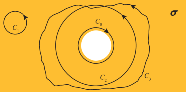
Figure 2: A closed 1-form $\bm{\sigma}$ in the punctured plane $\mathbb{R}^{2}\backslash\{0\}$. By Stokes’ theorem, $\oint_{C_{1}}\bm{\sigma}=0$ and $\oint_{C_{2}}\bm{\sigma}=\oint_{C_{3}}\bm{\sigma}$.

$$\int_{C_{2}\sqcup C_{0}}\bm{\sigma}\equiv\oint_{C_{2}}\bm{\sigma}+\oint_{C_{0}}\bm{\sigma}\ =\ \int_{C_{3}\sqcup C_{0}}\bm{\sigma}\ \ \ \Rightarrow\ \ \ \oint_{C_{2}}\bm{\sigma}=\oint_{C_{3}}\bm{\sigma}\ .$$

So, the circulation of $\bm{\sigma}$ vanishes along any loop not enclosing the origin (“hole”), and has the same value for any loop enclosing it. When $\oint_{C_{2}}\bm{\sigma}=\oint_{C_{3}}\bm{\sigma}\neq 0$, the form $\bm{\sigma}$ is non-exact; an example is the 1-form $\bm{\sigma}=\mathbf{d}\phi$.

2.4 Komar Integrals

In stationary spacetimes admitting Killing vectors fields $\xi^{\alpha}$, and for a compact spacelike hypersurface (i.e., 3-volume) $\mathcal{V}$ with boundary $\partial\mathcal{V}$, the Komar integrals are defined as [34, 35, 36, 37, 38]

$$Q_{\xi}(\mathcal{V})=-\frac{K}{16\pi}\int_{\partial\mathcal{V}}\star\mathbf{d}\bm{\xi}\ ,$$ (14)

where $(\star\mathbf{d}\bm{\xi})_{\alpha\beta}\equiv\xi_{\nu;\mu}\epsilon_{\ \ \alpha\beta}^{\mu\nu}$ is the 2-form dual to $\mathbf{d}\bm{\xi}$, and $K$ a dimensionless constant specific to each $\xi^{\alpha}$. Since $\mathcal{V}$ is compact, an application of the Stokes theorem leads to the equivalent expressions

$$Q_{\xi}(\mathcal{V})=-\frac{K}{16\pi}\int_{\mathcal{V}}\mathbf{d}(\star\mathbf{d}\bm{\xi})=\frac{K}{8\pi}\int_{\mathcal{V}}R_{\ \beta}^{\alpha}\xi^{\beta}d\mathcal{V}_{\alpha}=-K\int_{\mathcal{V}}\left[T_{\ \beta}^{\alpha}-\frac{1}{2}g_{\ \beta}^{\alpha}T_{\ \gamma}^{\gamma}\right]\xi^{\beta}n_{\alpha}d\mathcal{V},$$ (15)

where $d\mathcal{V}_{\alpha}=-n_{\alpha}d\mathcal{V}=\epsilon_{\alpha\mu\nu\lambda}\mathbf{d}x^{\mu}\wedge\mathbf{d}x^{\nu}\wedge\mathbf{d}x^{\lambda}/6$ is the volume element 1-form of $\mathcal{V}$, $n^{\alpha}$ is the future-pointing unit vector normal to $\mathcal{V}$, and we used the well known relation for Killing vectors fields $\xi_{\ ;\delta\alpha}^{\alpha}=R_{\beta\delta}\xi^{\beta}$ to notice that $\mathbf{d}(\star\mathbf{d}\bm{\xi})=-2R_{\alpha\beta}\xi^{\beta}d\mathcal{V}^{\alpha}$. Observe that this expression implies that, in vacuum ($R_{\mu\nu}=0$), $\star\mathbf{d}\bm{\xi}$ is a closed 2-form. Via the Stokes theorem, this means that $Q_{\xi}(\mathcal{V})=0$ for any compact hypersurface $\mathcal{V}$ not enclosing sources, and has the same value for any compact $\mathcal{V}$ enclosing an isolated system (see Sec. 2.3 above). Due to this hypersurface independence, $Q_{\xi}(\mathcal{V})$ is said to be conserved.

In an asymptotically flat axistationary spacetime, and in a suitable coordinate system [34, 39, 36], where the Killing vector field $\partial_{t}^{\alpha}=\xi^{\alpha}$ is time-like and tangent to inertial observers at infinity (corresponding to the source’s asymptotic inertial “rest” frame), and is moreover normalized so that $\xi^{\alpha}\xi_{\alpha}\stackrel{{\scriptstyle r\rightarrow\infty}}{{\rightarrow}}-1$, the quantity $M=Q_{\xi}(\mathcal{V})$, with $K=-2$, has the physical meaning of “active gravitational mass,” or total mass/energy present in the spacetime [34, 39, 37, 36]. Similarly, $J=Q_{\zeta}(\mathcal{V})$, for $\zeta^{\alpha}=\partial_{\phi}^{\alpha}$ and $K=1$, is the angular momentum present in the spacetime. Other coordinate systems/Killing vectors can be considered; in that case, however, the interpretation of quantities such as mass or angular momentum is in general not appropriate. Consider, e.g., a rigidly rotating coordinate system $\{x^{\alpha^{\prime}}\}$, obtained from the asymptotically inertial coordinate system $\{x^{\alpha}\}$ by the transformation $\phi^{\prime}=\phi-\Omega^{\prime}t$, $x^{\alpha^{\prime}\neq\phi^{\prime}}=x^{\alpha}$. In terms of the new Killing vector field $\partial^{\prime}_{t}=\partial_{t}+\Omega^{\prime}\partial_{\phi}$, one has

$$M^{\prime}=\frac{1}{8\pi}\int_{\partial\mathcal{V}}\star\mathbf{d}\bm{\xi}^{\prime}=\frac{1}{8\pi}\int_{\partial\mathcal{V}}\star\mathbf{d}(\bm{\xi}+\Omega^{\prime}\bm{\zeta})=M-2\Omega^{\prime}J\ ,$$ (16)

i.e., $M^{\prime}$ is a mixture of the mass $M$ and the angular momentum $J$ of the spacetime (as computed in the asymptotically inertial frame). The latter in this case stays the same, $J^{\prime}=J$, as $\partial^{\prime}_{\phi^{\prime}}=\partial_{\phi}$.

3 Gravitomagnetism and its different levels

The gravitational effects generated by the motion of matter, or, more precisely, by mass/energy currents, are known as “gravitomagnetism”. The reason for the denomination is its many analogies with magnetism (generated by charge currents). To make them apparent, consider a stationary metric with line element written in the form (1), and let, as in (2), $u^{\alpha}$ be the 4-velocity of the laboratory observers, and $U^{\alpha}=dx^{\alpha}/d\tau$ the 4-velocity of a test point particle in geodesic motion. The space components of the geodesic equation $DU^{\alpha}/d\tau=0$ yield [10, 13, 40, 31, 15]

$$\frac{\tilde{D}\vec{U}}{d\tau}=\gamma\left[\gamma\vec{G}+\vec{U}\times\vec{H}\right]$$ (17)

where $\gamma=-U^{\alpha}u_{\alpha}=e^{\Phi}(U^{0}-U^{i}\mathcal{A}_{i})$ is the Lorentz factor between $U^{\alpha}$ and $u^{\alpha}$,

$$\left[\frac{\tilde{D}\vec{U}}{d\tau}\right]^{i}=\frac{dU^{i}}{d\tau}+\Gamma(h)_{jk}^{i}U^{j}U^{k}\ ;\qquad\Gamma(h)_{jk}^{i}=\frac{1}{2}h^{il}\left(h_{lj,k}+h_{lk,j}-h_{jk,l}\right)$$ (18)

is a covariant derivative with respect to the spatial metric $h_{ij}$, with $\Gamma(h)_{jk}^{i}$ the corresponding Christoffel symbols, and

$$\vec{G}=-\tilde{\nabla}\Phi\ ;\qquad\quad\vec{H}=e^{\Phi}\tilde{\nabla}\times\vec{\mathcal{A}}\ ,$$ (19)

are vector fields living on the space manifold $\Sigma$ with metric $h_{ij}$, dubbed, respectively, “gravitoelectric” and “gravitomagnetic” fields. These play in Eq. (17) roles analogous to those of the electric ($\vec{E}$) and magnetic ($\vec{B}$) fields in the Lorentz force equation, $DU^{i}/d\tau=(q/m)[\gamma\vec{E}+\vec{U}\times\vec{B}]^{i}$. Here $\tilde{\nabla}$ denotes covariant differentiation with respect to the spatial metric $h_{ij}$ [i.e., the Levi-Civita connection of $(\Sigma,h)$]. Notice that Eq. (18) is the standard covariant expression for the 3-D acceleration (e.g. Eq. (6.9) in [41]); equation (17) describes the acceleration of the curve obtained by projecting the time-like geodesic onto the space manifold $(\Sigma,h)$, and $\vec{U}$ is its tangent vector [identified in spacetime with the projection of $U^{\alpha}$ onto $(\Sigma,h)$: $(\vec{U})^{\alpha}=h_{\ \beta}^{\alpha}U^{\beta}$, cf. Eq. (3)]. The physical interpretation of Eq. (17) is that, from the point of view of the laboratory observers, the spatial trajectory will seem to be accelerated, as if acted by fictitious forces—inertial forces. These arise from the fact that the laboratory frame is not inertial; in fact, $\vec{G}$ and $\vec{H}$ are identified in spacetime, respectively, with minus the acceleration and twice the vorticity (12) of the laboratory observers:

$$G^{\alpha}=-\nabla_{\mathbf{u}}u^{\alpha}\equiv-u_{\ ;\beta}^{\alpha}u^{\beta}\;;\qquad H^{\alpha}=\epsilon^{\alpha\beta\gamma\delta}u_{\gamma;\beta}u_{\delta}\;.$$ (20)

One may cast $\vec{G}$ as a relativistic generalization of the Newtonian gravitational field (embodying it as a limiting case), and $\vec{H}$ as a generalization of the Coriolis field [42]. Equations (17)-(19) apply to stationary spacetimes (being part of the so-called 1+3 “quasi-Maxwell” formalism [10, 13, 40, 31, 43, 15]); formulations for arbitrary spacetimes are given in [31, 12, 11, 44].

Since $\vec{B}=\nabla\times\vec{A}$ and, in stationary settings, $\vec{E}=-\nabla\phi$, Eqs. (19) suggest also an analogy between the electric potential $\phi$ and the “Newtonian” potential $\Phi$, and between the magnetic potential vector $\vec{A}$ and the vector $\vec{\mathcal{A}}$ (which, as seen in Sec. 2.2, governs the Sagnac effect); for this reason $\vec{\mathcal{A}}$ is dubbed gravitomagnetic vector potential.

Other realizations of the analogy exist, namely in the equations of motion for a “gyroscope” (i.e., a spinning pole-dipole particle) in a gravitational field and a magnetic dipole in a electromagnetic field. According to the Mathisson-Papapetrou equations [45, 46, 47, 48, 49, 50], under the Mathisson-Pirani spin condition [45, 51], the spin vector of a gyroscope of 4-velocity $U^{\alpha}$ evolves as $DS^{\alpha}/d\tau=S^{\mu}a_{\mu}U^{\alpha}$; here $a^{\alpha}\equiv DU^{\alpha}/d\tau$ and $S^{\alpha}$ is the spin vector, which is spatial with respect to $U^{\alpha}$ ($S^{\alpha}U_{\alpha}=0$). For a gyroscope whose center of mass is at rest in the coordinate system of (1), $U^{\alpha}=u^{\alpha}$ [see Eq. (2)], and the space part of the spin evolution equation reads (see footnote on page 5, and notice that $S^{\alpha}u_{\alpha}=0\Rightarrow S^{0}=S^{i}\mathcal{A}_{i}$)

$$\frac{d\vec{S}}{d\tau}=\frac{1}{2}\vec{S}\times\vec{H}\ ,$$ (21)

which is analogous to the precession of a magnetic dipole in a magnetic field, $D\vec{S}/d\tau=\vec{\mu}\times\vec{B}$. Another effect directly governed by the gravitomagnetic field $\vec{H}$ is the Sagnac time delay in an optical gyroscope, as follows from Eqs. (13),

$$\Delta t\approx 2e^{-\Phi}\vec{H}\cdot\vec{{\rm A}}\!{\rm rea}_{\mathcal{S}}\ ;\qquad\Delta\tau\approx 2\vec{H}\cdot\vec{{\rm A}}\!{\rm rea}_{\mathcal{S}}\ .$$ (22)

When the electromagnetic field is non-homogeneous, a force is exerted on a magnetic dipole, covariantly described by $DP^{\alpha}/d\tau=B^{\beta\alpha}\mu_{\beta}$ [50, 48], where $\mu^{\beta}$ is the magnetic dipole moment 4-vector, and $B_{\alpha\beta}=\star F_{\alpha\mu;\beta}U^{\mu}$ ($F^{\alpha\beta}\equiv$ Faraday tensor, $\star\equiv$ Hodge dual) is the “magnetic tidal tensor” as measured by the particle. A covariant force is likewise exerted on a gyroscope in a gravitational field (the spin-curvature force [45, 46, 47, 48, 49, 50]), which (again, under the Mathisson-Pirani spin condition) takes a remarkably similar form [50, 52]

$$\frac{DP^{\alpha}}{d\tau}=-\mathbb{H}^{\beta\alpha}S_{\beta};\qquad\quad\mathbb{H}_{\alpha\beta}\equiv\star R_{\alpha\mu\beta\nu}U^{\mu}U^{\nu}=\frac{1}{2}\epsilon_{\alpha\mu}^{\ \ \ \lambda\tau}R_{\lambda\tau\beta\nu}U^{\mu}U^{\nu}.$$ (23)

Here $\mathbb{H}_{\alpha\beta}$ is the “gravitomagnetic tidal tensor” (or “magnetic part” of the Riemann tensor [53]) as measured by the particle, playing a role analogous to that of $B_{\alpha\beta}$ in electromagnetism. For a congruence of observers at rest in a stationary field in the form (1), the relation between these tidal tensors and the magnetic/gravitomagnetic fields is [31]

$$B_{ij} = \tilde{\nabla}_{j}B_{i}+\frac{1}{2}\left[\vec{E}\cdot\vec{H}h_{ij}-E_{j}H_{i}\right]\ ;$$ (24)

$$\mathbb{H}_{ij} = -\frac{1}{2}\left[\tilde{\nabla}_{j}H_{i}+(\vec{G}\cdot\vec{H})h_{ij}-2G_{j}H_{i}\right]\ .$$ (25)

In a locally inertial frame (and rectangular coordinates) $B_{ij}=B_{i,j}$, and the force on a comoving magnetic dipole reduces to the textbook expression $DP^{i}/d\tau=B^{j,i}u_{j}\equiv\nabla(\vec{\mu}\cdot\vec{B})$. Moreover, in the linear regime, $\mathbb{H}_{ij}\approx H_{i,j}$, and so the force (23) on a gyroscope at rest yields $D\vec{P}/d\tau\approx\nabla(\vec{S}\cdot\vec{H})/2$. The tidal tensors $B_{\alpha\beta}$ and $\mathbb{H}_{\alpha\beta}$ are essentially quantities one order higher in differentiation, comparing to the corresponding fields $B^{\alpha}$ and $H^{\alpha}$. The gravitoelectric counterpart of $\mathbb{H}_{\alpha\beta}$ is the tidal tensor $\mathbb{E}_{\alpha\beta}\equiv R_{\alpha\mu\beta\nu}U^{\mu}U^{\nu}$ (“electric part” of the Riemann tensor) [52, 31], which governs the geodesic deviation equation $D^{2}\delta x^{\alpha}/d\tau=-\mathbb{E}_{\ \beta}^{\alpha}\delta x^{\beta}$. In vacuum, these tensors together fully determine the Riemann (i.e. Weyl) tensor, cf. the decomposition (30) of [54], and hence the tidal forces felt by any set of test particles/observers.

Levels of Magnetism		Levels of Gravitomagnetism
Governing Field	Physical effect	Governing Field	Physical effect
$\vec{A}$ (magnetic vector potential)	$\bullet$ Aharonov-Bohm effect     (quantum theory)	$\vec{\mathcal{A}}$ (gravitomagnetic vector potential)	$\bullet$ Sagnac effect $\bullet$ part of gravitomagnetic     “clock effect”
$\vec{B}$ (magnetic field $=\nabla\times\vec{A}$)	$\bullet$ magnetic force    $q\vec{U}\times\vec{B}$ $\bullet$ dipole precession    $D\vec{S}/d\tau=\vec{\mu}\times\vec{B}$ $\bullet$ magnetic “clock    effect”	$\vec{H}$ (gravitomagnetic field $=e^{\phi}\nabla\times\vec{\mathcal{A}}$)	$\bullet$ gravitomagnetic force    $m\gamma\vec{U}\times\vec{H}$ $\bullet$ gyroscope precession    $d\vec{S}/d\tau=\vec{S}\times\vec{H}/2$ $\bullet$ Sagnac effect in    light gyroscope $\bullet$ part of gravitomagnetic     “clock effect”
$B_{\alpha\beta}$ (magnetic tidal tensor $\sim\partial_{i}\partial_{j}A_{k}$)	$\bullet$ Force on mag. dipole    $DP^{\alpha}/d\tau=B^{\beta\alpha}\mu_{\beta}$	$\mathbb{H}_{\alpha\beta}$ (gravitomagnetic tidal tensor $\sim\partial_{i}\partial_{j}\mathcal{A}_{k}$)	$\bullet$ Force on gyroscope    $DP^{\alpha}/d\tau=-\mathbb{H}^{\beta\alpha}S_{\beta}$

Table 1: Levels of magnetism and gravitomagnetism, corresponding to different levels of differentiation of, respectively, the magnetic ($\vec{A}$) and gravitomagnetic ($\vec{\mathcal{A}}$) vector potentials.

The analogy between magnetic and gravitomagnetic effects can thus be cast into the three distinct levels in Table 1, corresponding to three different levels of differentiation of the gravitomagnetic vector potential $\vec{\mathcal{A}}$.

We close this overview with a note on the so-called “frame dragging”; in the literature this denomination is used for two main kinds of effects:

(i)

One, the fact that near a moving source (e.g. a rotating body) the compass of inertia, and thus the locally inertial frames, rotate with respect to inertial frames at infinity (i.e. to the “distant stars”). Or, conversely, near a rotating source a frame anchored to the distant stars in fact rotates with respect to the local compass of inertia [55, 56, 57, 58, 59, 28, 16, 18, 42], and observers at rest therein have non-vanishing vorticity [60, 61]. This is manifest in that, relative to such frame, gyroscopes precess [as described by Eq. (21)], and Coriolis (i.e. gravitomagnetic) forces arise [cf. Eq. (17)], causing e.g. orbits of test bodies to precess (Lense-Thirring orbital precession [55, 62, 63]), and the plane of a Foucault pendulum to rotate [16].

(ii)

The other, the fact that, close to a rotating source, the orbits of zero angular momentum (e.g. the ZAMOs of Sec. 2.1) have non-zero angular velocity as seen from infinity (or, conversely, objects with zero angular velocity have non-zero angular momentum) [16, 64, 65]. Associated to this, in axistationary spacetimes, a system of axes carried by the ZAMOs and spatially locked to the background symmetries (dubbed, somewhat misleadingly [16, 31], “locally non-rotating frames” [66, 67]), rotates with respect to comoving gyroscopes [68].

We point out, in view of the above, that the phenomena in (i) and (ii) have distinct origins, corresponding to two different levels of gravitomagnetism, the former being governed by $\vec{H}$, and the latter by $\vec{\mathcal{A}}$. The effects are independent: in fact, as we shall see, there exist solutions for which $\vec{H}$ vanishes whilst $\vec{\mathcal{A}}$ is non-zero, of which the metric in Sec. 5.2.2 is an example.

3.1 The gravitomagnetic clock effect

When a body rotates, the period of co- and counter-rotating geodesics around it differs in general; such effect has been dubbed [69, 70, 71, 72] gravitomagnetic “clock effect”. Let $U^{\alpha}\equiv dx^{\alpha}/d\tau=U^{0}\delta_{0}^{\alpha}+U^{\phi}\delta_{\phi}^{\alpha}$ be the 4-velocity of a test particle describing a circular geodesic in an axistationary spacetime, and $\mathcal{L}=g_{\mu\nu}U^{\mu}U^{\nu}/2$ the corresponding Lagrangian. The angular velocity $\Omega_{{\rm geo}}\equiv d\phi/dt=U^{\phi}/U^{0}$ of the circular geodesics is readily obtained from the Euler-Lagrange equations,

$$\frac{d}{d\tau}\left(\frac{\partial\mathcal{L}}{\partial U^{\alpha}}\right)-\frac{\partial\mathcal{L}}{\partial x^{\alpha}}=0\ ,$$ (26)

which reduce to

$$g_{\phi\phi,r}\Omega_{{\rm geo}}^{2}+2g_{0\phi,r}\Omega_{{\rm geo}}+g_{00,r}=0\ .$$ (27)

Solving this equation yields

$$\Omega_{{\rm geo}\pm}=\frac{-g_{0\phi,r}\pm\sqrt{g_{0\phi,r}^{2}-g_{\phi\phi,r}g_{00,r}}}{g_{\phi\phi,r}}$$ (28)

the $+$ ($-$) sign corresponding, for $g_{\phi\phi,r}>0$ and $g_{00,r}<0$ (i.e., attractive $\vec{G}$), to prograde (retrograde) geodesics, i.e., positive (negative) $\phi$ directions. The orbital period is, in coordinate time, $t_{{\rm geo}}=2\pi/|\Omega_{{\rm geo}}|$; hence, the difference between the periods of prograde and retrograde geodesics reads

$$\Delta t_{{\rm geo}}=2\pi\left(\frac{1}{\Omega_{{\rm geo+}}}+\frac{1}{\Omega_{{\rm geo-}}}\right)=-4\pi\frac{g_{0\phi,r}}{g_{00,r}}\ .$$

Since $g_{0\phi}=-g_{00}\mathcal{A}_{\phi}$, this result can be re-written as

$$\Delta t_{{\rm geo}}=4\pi\mathcal{A}_{\phi}-2\pi\frac{\mathcal{A}_{\phi,r}}{G_{r}}=4\pi\mathcal{A}_{\phi}-2\pi\frac{\star H_{r\phi}}{G_{r}e^{\Phi}}\ ,$$ (29)

where $\star H_{jk}\equiv\epsilon_{ijk}H^{i}$ is the 2-form dual to the gravitomagnetic field $\vec{H}$. In cylindrical coordinates one can substitute $\star H_{r\phi}=\sqrt{h}H^{z}$; in spherical coordinates, $\star\!H_{r\phi}=-\sqrt{h}H^{\theta}$. Hence, the gravitomagnetic clock effect consists of the sum of two contributions of different origin: the “global” Sagnac effect around the source, Eq. (10), which is governed by $\mathcal{A}_{\phi}$, plus a term governed by the gravitomagnetic field $\vec{H}$. The physical interpretation of the latter is as follows: for circular orbits, the gravitomagnetic force $\gamma\vec{U}\times\vec{H}$ in Eq. (17) is radial (since $\vec{H}$ is parallel to the axis, and $\vec{U}=U^{\phi}\partial_{\phi}$), being attractive or repulsive depending on the $\pm\phi$ direction of the orbit. Namely, it is attractive when the test body counter-rotates with the central source, and repulsive when it co-rotates. This highlights the fact that (anti-) parallel mass/energy currents have a repulsive (attractive) gravitomagnetic interaction, which is opposite to the situation in electromagnetism, where (anti-) parallel charge currents attract (repel) (see [73] and Sec. 13.6 of [74], respectively, for enlightening analogous explanations of these relativistic effects). In fact, the second term has an exact electromagnetic analogue, as we shall now show.

Electromagnetic analogue

Consider, in flat spacetime, a charged test particle of charge $q$ and mass $m$ in a circular orbit around a spinning charged body, and let $\mathcal{L}=mg_{\mu\nu}U^{\mu}U^{\nu}/2+qg_{\mu\nu}U^{\mu}A^{\nu}$, with $A^{\mu}=(\phi,\vec{A})$, be the corresponding Lagrangian. The Euler-Lagrange equations (26) yield, for a circular orbit,

$$qE_{r}+q\Omega_{{\rm orb}}A_{\phi,r}+\frac{1}{2}U^{0}mg_{\phi\phi,r}\Omega_{{\rm orb}}^{2}=0\ ,$$

where $\Omega_{{\rm orb}}\equiv d\phi/dt=U^{\phi}/U^{0}$, leading to

$$\Omega_{{\rm orb\pm}}=\frac{-qA_{\phi,r}\pm\sqrt{q^{2}A_{\phi,r}^{2}-2U^{0}qmg_{\phi\phi,r}E_{r}}}{U^{0}mg_{\phi\phi,r}}\ .$$

Thus, for $qE_{r}<0$ (attractive electric force), the difference between the periods of prograde and retrograde orbits is

$$\Delta t_{{\rm orb}}=2\pi\left(\frac{1}{\Omega_{{\rm orb+}}}+\frac{1}{\Omega_{{\rm orb-}}}\right)=-\frac{2\pi A_{\phi,r}}{E_{r}}=-2\pi\frac{\star B_{r\phi}}{E_{r}}\ ,$$ (30)

where $\star B_{jk}\equiv\epsilon_{ijk}B^{i}$ is the 2-form dual to the magnetic field $\vec{B}$ (not to be confused with the magnetic tidal tensor $B_{\alpha\beta}$). In cylindrical coordinates, $\star B_{r\phi}=B^{z}$; in spherical coordinates, $\star B_{r\phi}=-B^{\theta}$. Notice the analogy with Eq. (29), identifying $\{\vec{E},\ \vec{B}\}\leftrightarrow\{\vec{G},\ \vec{H}\}$. We can thus say that the gravitomagnetic clock effect in Eq. (29) consists of a term with a direct electromagnetic analogue, plus a term (the Sagnac time delay $4\pi\mathcal{A}_{\phi}$) that has no electromagnetic counterpart in Eq. (30).

Observer-independent “two-clock” effect

The time delay (29) corresponds to orbital periods as seen by the laboratory observers (2), and measured in coordinate time [which can be converted into observer’s proper time via Eq. (9)]. Other observers, rotating with respect to the laboratory observers, will measure different periods, since, from their point of view, the closing of the orbits occurs at different points. The effect can also be formulated in terms of the orbital proper times [69, 75, 76] (“two clock effect”); for a discussion of such alternative formulations and their relationships, we refer to [71]. An observer independent clock effect can however be derived, based on the proper times ($\tau_{+}$ and $\tau_{-}$) measured by each orbiting clock between the events where they meet [77]. Consider two oppositely rotating circular geodesics at some fixed $r$, and set a starting meeting point at $\phi_{+}=\phi_{-}=0$, $t=0$. The next meeting point is defined by $\phi_{+}=2\pi+\phi_{-}$. Since $\phi_{\pm}=\Omega_{{\rm geo}\pm}t$, the meeting point occurs at a coordinate time $t=2\pi/(\Omega_{{\rm geo}+}-\Omega_{{\rm geo}-})$. Since $dt/d\tau_{\pm}=U_{\pm}^{0}$, and

$$U_{\pm}^{0}=\left[-g_{00}-2\Omega_{{\rm geo}\pm}g_{0\phi}-\Omega_{{\rm geo}\pm}^{2}g_{\phi\phi}\right]^{-1/2}$$ (31)

is constant along a circular orbit, it follows that $\tau_{\pm}=t/U_{\pm}^{0}$, thus

$$\tau_{\pm}=\frac{2\pi(U_{\pm}^{0})^{-1}}{\Omega_{{\rm geo}+}-\Omega_{{\rm geo}-}}\ ;\qquad\quad\Delta\tau\equiv\tau_{+}-\tau_{-}=2\pi\frac{(U_{+}^{0})^{-1}-(U_{-}^{0})^{-1}}{\Omega_{{\rm geo}+}-\Omega_{{\rm geo}-}}\ .$$ (32)

4 The electromagnetic analogue: the field of an infinite rotating charged cylinder

Consider, in flat spacetime, a charged, infinitely long rotating cylinder along the $z-$axis. Its exterior electromagnetic field is described (cf. e.g. [74]) by the 4-potential 1-form $A_{\alpha}=(-\phi,\mathbf{A})$,

$$\phi=-2\lambda\ln(r/r_{0})\ ;\qquad\mathbf{A}=A_{\phi}\mathbf{d}\phi=2\mathfrak{m}\mathbf{d}\phi\qquad(\vec{A}=\frac{2\mathfrak{m}}{r^{2}}\partial_{\phi})\ ,$$ (33)

where $\phi\equiv\phi(r)$ is the electric potential, $r_{0}$ is an arbitrary constant, $\vec{A}$ is the (3-D) magnetic vector potential (with associated 1-form $\mathbf{A}$), and $\lambda$ and $\mathfrak{m}$ are, respectively, the charge and magnetic moment per unit $z-$length. The corresponding electric and magnetic fields read

$$\vec{E}=-\nabla\phi=\frac{2\lambda}{r}\partial_{r}\ ;\qquad\vec{B}=\nabla\times\vec{A}=0\ .$$ (34)

The magnetic tidal tensor $B_{\alpha\beta}$ also vanishes trivially since $\vec{H}=0$ for an inertial frame, cf. Eq. (24). Hence, the electromagnetic field of a rotating cylinder differs from that of a static one only in the vector potential $\vec{A}$, which vanishes in the latter case ($\mathfrak{m}=0$).

4.1 Aharonov-Bohm effect

Classically, the physics in the exterior field of a rotating cylinder are the same as for a static one, since $\vec{A}$ itself plays no role in any physical process (only its curl $\vec{B}$). In other words, classically, an irrotational vector potential $\vec{A}$ is pure gauge. Quantum theory, however, changes the picture, since $\vec{A}$ intervenes physically in the so-called Aharonov-Bohm effect [78]. This effect can be described as follows. The wave function of a particle of charge $q$ moving in a stationary electromagnetic field along a spatial path $C$ acquires a phase shift given by $\varphi=q/\hbar\int_{C}\mathbf{A}\equiv q/\hbar\int_{C}\vec{A}\cdot d\vec{l}$ [78]. Now consider, as in Fig. 3, a beam of electrons which is split into two, each passing around a rotating charged cylinder but on opposite sides (while avoiding it). Since $\vec{A}$ circulates around the cylinder, that will lead to a phase difference between the beams, which manifests itself in a shift of the interference pattern when the beams are recombined.

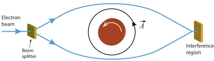
Figure 3: Simplified scheme for the Aharonov-Bohm effect around a rotating charged cylinder.

Let $\varphi_{+}$ ($\varphi_{-}$) denote the phase shift induced in the beam propagating in the same (opposite) sense of the cylinder’s rotation. Since the field lines of $\vec{A}$ are circles around the cylinder, the phase shifts in the two paths are of equal magnitude but opposite sign: $\varphi_{+}=-\varphi_{-}$. The two paths together form a closed loop; since $\nabla\times\vec{A}=0$ outside the cylinder, by the Stokes theorem $\int_{C}\mathbf{A}$ is the same for every closed spatial loop $C$ enclosing the cylinder (in particular, a circular one); hence, the phase difference between the two paths, $\Delta\varphi=\varphi_{+}-\varphi_{-}$, equals the phase shift along any circular loop $C$ enclosing the cylinder

$$\Delta\varphi=\frac{q}{\hbar}\oint_{C}\mathbf{A}=\frac{q}{\hbar}A_{\phi}\int_{0}^{2\pi}d\phi=\frac{2\pi q}{\hbar}A_{\phi}\ .$$ (35)

Notice the formal analogy with the expression (10) for the Sagnac effect on a circular loop around the axis of an axistationary metric: $\Delta t$ therein corresponds to a difference in beam arrival times for one full loop; for a half loop [as is the case in Eq. (35)] the time difference is $\Delta t/2$, corresponding to a phase difference $\Delta\varphi=(E/\hbar)\Delta t/2=(2\pi E/\hbar)\mathcal{A}_{\phi}$, where $E$ denotes the photon’s energy. Identifying $\{E,\mathcal{A}_{\phi}\}\leftrightarrow\{q,A_{\phi}\}$, this exactly matches (35).

For comparison with the gravitational analogue below, it is worth observing the following. The fact that $\int_{C}\mathbf{A}\neq 0$ for loops $C$ enclosing the cylinder is, in connection with Stokes’ theorem, assigned to the fact that, within the cylinder, $\nabla\times\vec{A}=\vec{B}\neq 0$. However, one could as well restrict our analysis to the region outside the cylinder (as originally done in [78]); that is, cut the cylinder out of the space manifold, and consider the field $\vec{A}$ defined in the multiply connected region thereby obtained. The fact that $\int_{C}\mathbf{A}\neq 0$, in spite of $\mathbf{d}\mathbf{A}=0$ everywhere, is then explained through the fact that $C$ lies in a region which is not simply connected [6], where $\mathbf{A}$ is a closed but non-exact form: in this case Stokes’ theorem does not require its circulation to vanish, but only to have the same value $2\pi A_{\phi}$ for any closed loop $C$ around the cylindrical hole, cf. Sec. 2.3.

4.2 Rotating frame

Consider the coordinate system $\{x^{\bar{\alpha}}\}$, obtained from the globally inertial coordinate system $\{x^{\alpha}\}$ by the transformation $x^{\bar{i}\neq\bar{\phi}}=x^{i}$, $\bar{\phi}=\phi-\Omega t$, corresponding to a reference frame rotating with angular velocity $\Omega$ about the cylinder’s axis. The Minkowski metric in such coordinates reads

$$ds^{2}=(-1+\Omega^{2}r^{2})dt^{2}+dr^{2}+2\Omega r^{2}dtd\bar{\phi}+dz^{2}+r^{2}d\bar{\phi}^{2}\ .$$ (36)

The 4-potential 1-form $A_{\bar{\alpha}}=\Lambda_{\ \bar{\alpha}}^{\beta}A_{\beta}$ ($\Lambda_{\ \bar{\alpha}}^{\beta}\equiv\partial x^{\beta}/\partial x^{\bar{\alpha}}$) becomes, in such coordinates, $A_{\bar{\alpha}\neq\bar{t}}=A_{\alpha}$, $A_{\bar{t}}=-\phi+A_{\phi}\Omega$. The electric and magnetic fields are given by $\bar{E}^{\bar{\alpha}}=F^{\bar{\alpha}\bar{\beta}}\bar{u}_{\bar{\beta}}$ and $\bar{B}^{\bar{\alpha}}=\star F^{\bar{\alpha}\bar{\beta}}\bar{u}_{\bar{\beta}}$, where $F_{\alpha\beta}\equiv 2A_{[\beta,\alpha]}=2A_{[\beta;\alpha]}$ is the Faraday 2-form and $\bar{u}^{\bar{\alpha}}=(-g_{\bar{0}\bar{0}})^{-1/2}\delta_{\bar{0}}^{\bar{\alpha}}$ is the 4-velocity of the observers at rest in the rotating coordinates; they read

$$\vec{\bar{E}}=\frac{2\lambda}{r\sqrt{1-r^{2}\Omega^{2}}}\partial_{r}\ ;\qquad\vec{\bar{B}}=\frac{2\Omega\lambda}{\sqrt{1-r^{2}\Omega^{2}}}\partial_{z}$$

($\bar{E}^{\bar{0}}=\bar{B}^{\bar{0}}=0$). So now a non-vanishing magnetic $\vec{\bar{B}}$ field arises.

Finally, observe that the curves of constant spatial coordinates $x^{\bar{i}}$, tangent to the Killing vector field $\partial_{\bar{t}}$, cease to be time-like for $r>1/\Omega$, since $g_{\bar{0}\bar{0}}>0$ therein. Hence, no observers $\bar{u}^{\bar{\alpha}}$, at rest with respect to such frame, can exist past that value of $r$ (they would exceed the speed of light).

5 Gravitational field of infinite rotating cylinders: the Lewis metrics

The exterior gravitational field of an infinitely long, rotating or non-rotating cylinder is generically described by the Lewis metric [3]

$$ds^{2}=-fdt^{2}+2kdtd\phi+r^{(n^{2}-1)/2}(dr^{2}+dz^{2})+ld\phi^{2}\ ;$$ (37)

$$f=ar^{1-n}-\frac{c^{2}r^{n+1}}{n^{2}a}\ ;\qquad k=-Cf\ ;\qquad l=\frac{r^{2}}{f}-C^{2}f\ ;\qquad C=\frac{cr^{n+1}}{naf}+b\ .$$ (38)

Here $a$, $b$, $c$, and $n$ are constants, which can be real or complex, corresponding, respectively, to the Weyl or Lewis classes of solutions. The constant $n$, in particular, is real for the Weyl class, and purely imaginary for the Lewis class [79, 80]. This is the most general stationary solution of the vacuum Einstein field equations with cylindrical symmetry. It encompasses, as special cases, the van Stockum [81] exterior solutions for the field produced by a rigidly rotating dust cylinder, and the static Levi-Civita metric, corresponding to a non-rotating cylinder.

Curvature invariants.— As is well known (e.g. [79, 33]), in vacuum there are four independent scalar invariants one can construct from the Riemann tensor (which equals the Weyl tensor): two quadratic, namely the Kretchmann and Chern-Pontryagin invariants, which read, for the metric (37),

$$\mathbf{R}\cdot\mathbf{R}\equiv R_{\alpha\beta\gamma\delta}R^{\alpha\beta\gamma\delta}=\frac{1}{4}(n^{2}-1)^{2}(3+n^{2})r^{-3-n^{2}};\qquad\star\!\mathbf{R}\cdot\mathbf{R}\equiv\star R_{\alpha\beta\gamma\delta}R^{\alpha\beta\gamma\delta}=0\ ,$$ (39)

plus the two cubic invariants

$$\mathbb{A} \equiv -\frac{1}{16}R_{\ \ \lambda\mu}^{\alpha\beta}R_{\ \ \ \rho\sigma}^{\lambda\mu}R_{\ \ \alpha\beta}^{\rho\sigma}=\frac{3}{256}(n^{2}-1)^{4}r^{-3(n^{2}+3)/2}\ ;$$ (40)

$$\mathbb{B} \equiv \frac{1}{16}R_{\ \ \lambda\mu}^{\alpha\beta}R_{\ \ \ \rho\sigma}^{\lambda\mu}\star\!R_{\ \ \alpha\beta}^{\rho\sigma}=0\ .$$ (41)

5.1 Gravitoelectromagnetic (GEM) fields and tidal tensors

The metric (37)-(38) can be put in the form (4), with

$$e^{2\Phi}=f;\qquad\mathcal{A}_{\phi}=-\frac{cr^{n+1}}{naf}-b\ ;\qquad h_{rr}=h_{zz}=r^{(n^{2}-1)/2};\qquad h_{\phi\phi}=r^{2}e^{-2\Phi},$$ (42)

and $h_{ij}=0$ for $i\neq j$. The gravitoelectric and gravitomagnetic fields read, cf. Eqs. (19),

$$G_{i}=\frac{a^{2}(n-1)n^{2}+c^{2}(1+n)r^{2n}}{2r(a^{2}n^{2}-c^{2}r^{2n})}\delta_{i}^{r};\qquad\vec{H}=\frac{2acn^{2}r^{-(n-1)^{2}/2}}{c^{2}r^{2n}-a^{2}n^{2}}\partial_{z}\ .$$ (43)

Equation (17) then tells us that test particles in geodesic motion are, from the point of view of the reference frame associated to the coordinate system of (37), acted upon by two inertial forces: a radial force (per unit mass) $\gamma^{2}\vec{G}$, which can be attractive or repulsive (depending on $n$, $a$, and $c$), and a gravitomagnetic force (per unit mass) $\gamma\vec{U}\times\vec{H}$, likewise lying on the plane orthogonal to the cylinder. A consequence of the latter is that test particles dropped from rest are deflected sideways, instead of moving radially. The non-vanishing $\vec{H}$ means also that gyroscopes precess relative to the frame associated to the coordinates of (37), cf. Eq. (21).

The non-vanishing components of the gravitoelectric $\mathbb{E}_{\alpha\beta}\equiv R_{\alpha\mu\beta\nu}u^{\mu}u^{\nu}$ and gravitomagnetic $\mathbb{H}_{\alpha\beta}\equiv\star R_{\alpha\mu\beta\nu}u^{\mu}u^{\nu}$ tidal tensors as measured by the observers at rest in the coordinates of (37) read

$$\mathbb{E}_{rr} = -(1-n^{2})\frac{a^{2}n^{2}(n+1)+c^{2}(n-1)r^{2n}}{8r^{2}(a^{2}n^{2}-c^{2}r^{2n})}\ ;\qquad\mathbb{E}_{\phi\phi}=(1-n^{2})\frac{an^{2}r^{-(n-1)^{2}/2}}{4(a^{2}n^{2}-c^{2}r^{2n})}\ ;$$

$$\mathbb{E}_{zz} = (1-n^{2})\frac{a^{2}n^{2}(n-1)+c^{2}(n+1)r^{2n}}{8r^{2}(a^{2}n^{2}-c^{2}r^{2n})}\ ,$$ (44)

$$\mathbb{H}_{rz}=\mathbb{H}_{zr}=-\frac{(1-n^{2})acn^{2}r^{n-2}}{4(c^{2}r^{2n}-a^{2}n^{2})}\ .$$ (45)

The fact that $\mathbb{H}_{\alpha\beta}\neq 0$ means that a spin-curvature force (23) is exerted on gyroscopes at rest in the coordinates of (37).

Comparing with the electromagnetic analogue, we observe that both the inertial and tidal fields (in particular the non-vanishing $\vec{H}$ and $\mathbb{H}_{\alpha\beta}$) are in contrast with the electromagnetic field of a rotating cylinder as measured in the inertial rest frame, discussed in Sec. 4, resembling more the situation in a rotating frame, discussed in Sec. 4.2.

5.1.1 The Levi-Civita static cylinder

It is known [3, 80] that when $n$ is real (Weyl class), and $b=0=c$, the metric (37) becomes

$$ds^{2}=-ar^{1-n}dt^{2}+r^{(n^{2}-1)/2}(dr^{2}+dz^{2})+\frac{r^{1+n}}{a}d\phi^{2}\ ,$$ (46)

which is the static Levi-Civita metric, corresponding to a non-rotating cylinder. Imposing $a>0$ (so that $t$ remains the time coordinate, and $\phi$ the spacelike periodic coordinate) yields, identifying the appropriate constants, a dimensionless version of the original line element in [82]. Further re-scaling the time coordinate $t\rightarrow a^{-1/2}t$, so that $g_{00}=-r^{1-n}$, yields the line element in the coordinate system in [83, 3, 2]. For this metric we have [cf. Eqs. (1), (19), (25)] $\mathcal{A}_{i}=\vec{H}=\mathbb{H}_{\alpha\beta}=0$, and

$$\Phi=\frac{1-n}{2}\ln(r)+K;\qquad G_{i}=-\Phi_{,i}=-\frac{1-n}{2r}\delta_{i}^{r}\ ,$$ (47)

where $K$ is an arbitrary constant (depending on the choice of units for $t$). That is, the Newtonian potential $\Phi$ and the gravitoelectric field 1-form $G_{i}$ exactly match, with the identification $(1-n)/4\leftrightarrow\lambda$, minus the electrostatic potential $\phi$ and electric field 1-form $E_{i}$ of the electromagnetic analogue in Sec. 4, cf. Eqs. (33)-(34). This analogy suggests identifying the quantity $(1-n)/4$ with the source’s mass density per unit $z-$length, in agreement with earlier interpretations (e.g. [84, 3, 76, 2]). The speed of the circular geodesics with respect to the coordinate system in (46) is

$$v_{{\rm geo}}=\sqrt{\frac{2}{1+n}-1}$$ (48)

(cf. e.g. [2]), which is independent of $r$ (like in the Newtonian/electric analogues, albeit with a different value). These are possible only when $0\leq n<1$ [85, 5, 86, 84, 87, 2], since $\vec{G}$ is attractive only for $n<1$, and their speed becomes superluminal for $n<0$.

5.1.2 The “force” parallel to the axis

In some literature [9, 2] it was found that test particles in geodesic motion appeared to be deflected by a rather mysterious “force” parallel to the cylinder’s axis. Let us examine the origin of such effect. It follows from Eqs. (17) and (43) that, in the reference frame associated to the coordinate system of (37), the only inertial forces acting on a test particle in geodesic motion are the radial gravitoelectric force $m\vec{G}$ and the gravitomagnetic force $m\gamma\vec{U}\times\vec{H}$ (with $\vec{H}$ parallel to the axis), both always orthogonal to the cylinder’s axis. It is thus clear that no axial inertial force exists. [In other words, the 3-D curve obtained by projecting the geodesic onto the space manifold $(\Sigma,h)$ has no axial acceleration, cf. Sec. 3]. The axial component of Eq. (17) reads

$$\frac{\tilde{D}U^{z}}{d\tau}=0\ \Leftrightarrow\ \frac{dU^{z}}{d\tau}=-2\Gamma(h)_{rz}^{z}U^{r}U^{z}=\frac{1-n^{2}}{2r}U^{r}U^{z}\ ,$$ (49)

which is Eq. (74) of [9]. That is, the coordinate “acceleration” $d^{2}z/d\tau^{2}\equiv dU^{z}/d\tau$ is down to the fact that the Christoffel symbol $\Gamma(h)_{rz}^{z}$ of the spatial metric $h_{ij}$ is non-zero. In particular, if $U^{z}\equiv dz/d\tau$ is initially zero, it actually remains zero along the motion. The question then arises on whether the effect is due to the curvature of the space manifold $(\Sigma,h)$ or to a coordinate artifact, as both are generically encoded in $\Gamma(h)_{jk}^{i}$. The distinction between the two is not clear in general (an example of a pure coordinate artifact is the variation of $U^{i}$ when one describes geodesic motion in flat spacetime using a non-Cartesian coordinate system, e.g. spherical coordinates). In the present case, however, the translational Killing vector $\partial_{z}$ gives us a notion of fixed axial direction; on the other hand, the dependence of $g_{zz}$ on $r$ (i.e., the fact that the magnitude $\sqrt{g_{zz}}$ of the basis vector $\partial_{z}$ is not constant along the particle’s trajectory) causes the coordinate acceleration $dU^{z}/d\tau$ to include a trivial coordinate artifact. Such effect is gauged away by switching to an orthonormal tetrad frame $\mathbf{e}_{\hat{\alpha}}$ such that $\mathbf{e}_{z}=(g_{zz})^{-1/2}\partial_{z}$, where the axial component of the 4-velocity reads $U^{\hat{z}}=U^{z}\sqrt{g_{zz}}$. It evolves as [using (49)] $dU^{\hat{z}}/d\tau=(1-n^{2})r^{(n^{2}-5)/4}U^{r}U^{z}/4$, which corresponds to the axial component of the geodesic equation written in such tetrad, $DU^{\hat{\alpha}}/d\tau=0$. Hence, even in an orthonormal frame $\mathbf{e}_{\hat{\alpha}}$, $U^{\hat{z}}$ is not constant; in other words, the axial vector component itself, $U^{z}\partial_{z}$ (not just the coordinate component $U^{z}$), varies along the particle’s motion. This is a consequence of the curvature of the space manifold. We conclude thus that $dU^{z}/d\tau$ in Eq. (49), interpreted in [9, 2] as an axial “force”, consists of a combination of a coordinate artifact caused by the variation of the basis vector $\partial_{z}$ along the particle’s trajectory, with a physical effect due to the curvature of the space manifold $(\Sigma,h)$.

5.2 The canonical form of the Weyl class

The Weyl class corresponds to all parameters in Eqs. (37)-(38) being real. We observe that, for $r^{2n}>a^{2}n^{2}/c^{2}$, the Killing vector field $\partial_{t}$ ceases to be time-like; thus no physical observers $u^{\alpha}=f^{-1/2}\partial_{t}^{\alpha}$, at rest in the coordinates of (37), can exist past that value of $r$. This resembles the situation for a rotating frame in flat spacetime, see Sec. 4.2. Moreover, the non-vanishing gravitomagnetic field $\vec{H}$ and tidal tensor $\mathbb{H}_{\alpha\beta}$, Eqs. (43) and (45), contrast with the electromagnetic problem of a charged rotating cylinder as viewed from the inertial rest frame (Sec. 4); they resemble instead the corresponding electromagnetic fields when measured in a rotating frame (Sec. 4.2). This makes one wonder whether these two features might be mere artifacts of some trivial rotation of the coordinate system in which the metric, in its usual form (37)-(38), is written. In what follows we shall argue this to be the case.

For the Weyl class, we have the invariant structure, cf. Eqs. (39)-(41): $\mathbf{R}\cdot\mathbf{R}>0$, $\star\!\mathbf{R}\cdot\mathbf{R}=0$, $\mathbb{B}=0$,

$$\mathbb{M}\equiv\frac{I^{3}}{(\mathbb{A}-i\mathbb{B})^{2}}-6=\frac{2n^{2}(n^{2}-9)^{2}}{9(n^{2}-1)^{2}}\geq 0\quad\mbox{(real)},$$ (50)

where $I\equiv(\mathbf{R}\cdot\mathbf{R}-i\star\!\mathbf{R}\cdot\mathbf{R})/8$. We shall see below (Secs. 5.2.1 and 5.2.3) that, in order for the cylinder’s Komar mass per unit length to be positive and its gravitational field attractive, while at the same time allowing for circular geodesics, it is necessary that $n^{2}<1$: for larger values of $|n|$ the physical significance of the solutions is unclear already in the static Levi-Civita special case, no longer representing the gravitational field of a cylindrical source [5, 83, 84, 85, 86, 87, 88, 2, 89, 90]. Moreover, for $n=0$ the metric coefficients diverge. We consider thus the range $0<n^{2}<1$ for solutions of physical interest to the problem at hand. In this case, $\mathbb{M}>0$; this, together with the above relations on the quadratic invariants, implies that the spacetime is purely “electric” [91, 33, 79, 92], i.e., everywhere there are observers for which the magnetic part of the Weyl tensor ($=\mathbb{H}_{\alpha\beta}$, in vacuum) vanishes. They imply also that the Petrov type is I, and thus at each point the observer measuring $\mathbb{H}_{\alpha\beta}=0$ is unique [33]. Let us find such observer congruence. The nontrivial components of the gravitomagnetic tidal tensor as measured by an observer of arbitrary 4-velocity $U^{\alpha}=(U^{t},U^{r},U^{\phi},U^{z})$ read ($\mathbb{H}_{\alpha\beta}=\mathbb{H}_{\beta\alpha})$:

$$\mathbb{H}_{tt} = \frac{\alpha cU^{r}U^{z}}{2r};\qquad\mathbb{H}_{tr}=\frac{\alpha(\beta U^{\phi}-2cU^{t})U^{z}}{8r};\qquad\mathbb{H}_{t\phi}=\frac{\alpha(2bc-n)U^{r}U^{z}}{4r};$$

$$\mathbb{H}_{tz} = \frac{\alpha\left[\chi U^{\phi}-2cU^{t}\right]U^{r}}{8r};\qquad\mathbb{H}_{r\phi}=\frac{\alpha\left[2b\xi U^{\phi}+\chi U^{t}\right]U^{z}}{8r};\qquad\mathbb{H}_{\phi\phi}=-\frac{\alpha b\xi U^{r}U^{z}}{2r};$$

$$\mathbb{H}_{rz} = \frac{\alpha(bU^{\phi}+U^{t})(cU^{t}-\xi U^{\phi})}{4r};\qquad\mathbb{H}_{\phi z}=\frac{\alpha\left[2b\xi U^{\phi}+\beta U^{t}\right]U^{r}}{8r},$$

where $\alpha\equiv 1-n^{2}$, $\beta\equiv n-2bc-3$, $\chi\equiv n-2bc+3$ and $\xi\equiv n-bc$. The condition $\mathbb{H}_{\alpha\beta}=0$ implies $U^{r}=U^{z}=0$, plus one of the following conditions:

$$\frac{U^{\phi}}{U^{t}}=-\frac{1}{b}\quad({\rm i})\qquad{\rm or}\qquad\frac{U^{\phi}}{U^{t}}=\frac{c}{n-bc}\ .\quad({\rm ii})$$ (51)

Notice that these conditions cannot hold simultaneously for 4-velocities $U^{\alpha}=U^{t}\partial_{t}^{\alpha}+U^{\phi}\partial_{\phi}^{\alpha}$: condition (51i) leads to a vector which is time-like iff $a<0$, whereas (51ii) leads to a vector which is time-like iff $a>0$. Hence, for any given values of the parameters ($a\neq 0$, $b$, $c$, $n$), there is one, and only one, congruence of observers for which $\mathbb{H}_{\alpha\beta}=0$; such congruence has 4-velocity

$$U^{\alpha}=U^{t}(\partial_{t}^{\alpha}+\Omega\partial_{\phi}^{\alpha})\ ;\qquad\Omega=\frac{c}{n-bc}\ \ {\rm for}\ a>0\ ;\qquad\Omega=-\frac{1}{b}\ \ {\rm for}\ a<0\ ,$$ (52)

consisting of observers rigidly rotating around the cylinder with constant angular velocity $\Omega\equiv U^{\phi}/U^{t}\equiv d\phi/dt$.

Since $\Omega$ is constant, by using the coordinate transformation

$$\bar{\phi}=\phi-\Omega t\ ;\qquad x^{\bar{\alpha}\neq\bar{\phi}}=x^{\alpha}$$ (53)

one can switch to a coordinate system where the observers (52) are at rest. In such a coordinate system, the metric (37) becomes

$$ds^{2}=-\bar{f}(dt+\bar{C}d\bar{\phi})^{2}+r^{(n^{2}-1)/2}(dr^{2}+dz^{2})+\frac{r^{2}}{\bar{f}}d\bar{\phi}^{2}\ ,$$ (54)

with, for $\Omega=c/(n-bc)$,

$$\bar{f}=\frac{r^{1-n}}{\alpha}\ ;\qquad\alpha=\frac{\bar{C}^{2}}{ab^{2}}\ ;\qquad\bar{C}=b\frac{n-bc}{n}\ ,$$ (55)

and, for $\Omega=-1/b$,

$$\bar{f}=\frac{r^{1+n}}{\alpha}\ ;\qquad\alpha=-ab^{2}\ ;\qquad\bar{C}=-b\frac{n-bc}{n}\ .$$ (56)

The special cases $bc=n$ and $b=0$, which are excluded from, respectively, the former and the latter transformations, both lead to the Levi-Civita line-element. That it is so for $b=0$ can be immediately seen by substituting in (54)-(55), yielding directly (46). This has previously been noticed in [76, 93], by a different route. That $n=bc$ also leads to the Levi-Civita metric (which seems to have gone unnoticed in the literature) can be seen by substituting $n\rightarrow bc$ in the expression for $\bar{C}$ in (56) and: (i), for $a<0$, by substituting in the remainder $n\equiv-m$, yielding (46) in a different notation (with $\{m,\alpha^{-1}\}$ in the place of $\{n,a\}$); (ii) for $a>0$, by substituting $\alpha=-|\alpha|$, yielding (46) with $t$ and $\phi^{\prime}$ swapped ($t$ the angular coordinate and $\phi^{\prime}$ the temporal coordinate, and $|\alpha|$ in the place of $a$).

Notice the simplicity of these forms of the metric, comparing to the usual form (37)-(38). In particular, we remark that $\bar{C}$ is a constant (we shall see below the importance of this result), and that these metrics depend only on three effective parameters: $\alpha$, $n$, and $\bar{C}$. This makes explicit the assertion in [4] that the four parameters ($a$, $b$, $c$, $n$) in the usual form of the metric are not independent. Observe moreover that, contrary to the situation in the usual form, the Killing vector $\partial_{t}$ is everywhere time-like, that is, $g_{00}<0$ for all $r$ [for $a>0$ in (55), and $a<0$ in (56)]. Therefore, physical observers $u^{\alpha}=\bar{f}^{-1/2}\partial_{t}^{\alpha}$, at rest in the coordinates of (54), exist everywhere (even for arbitrarily large $r$).

5.2.1 Komar Integrals

Infinite cylinders are not isolated sources, hence a conserved total mass or angular momentum (which is infinite) cannot be defined for bounded hypersurfaces. In these systems one can define instead a mass and angular momentum per unit length, obeying conservation laws analogous to those of $M$ and $J$ for finite sources. In order to effectively suppress the irrelevant $z-$coordinate from the problem, consider simply connected tubes $\mathcal{V}$ parallel to the $z-$axis, of unit $z-$length and arbitrary section. Let $\partial\mathcal{V}=\mathcal{S}\cup\mathcal{B}_{1}\cup\mathcal{B}_{2}$ be the boundary of such tubes, where $\mathcal{S}$ is the tube’s lateral surface, parameterized by $\{\phi,z\}$, and $\mathcal{B}_{1}$ and $\mathcal{B}_{2}$ its bases (of disjoint union $\mathcal{B}_{1}\sqcup\mathcal{B}_{2}$), lying in planes orthogonal to the $z-$axis and parametrized by $\{r,\phi\}$. Since, by the equation $\mathbf{d}(\star\mathbf{d}\bm{\xi})=-2R_{\alpha\beta}\xi^{\beta}d\mathcal{V}^{\alpha}$ (see Sec. 2.4), $\star\mathbf{d}\bm{\xi}$ is a closed form outside the cylinder, by the Stokes theorem the Komar integrals (14) vanish for all $\mathcal{V}$ exterior to the cylinder, and are the same for all $\mathcal{V}$ enclosing it. They are thus conserved quantities for such tubes. We can write

$$Q_{\xi}(\mathcal{V})=-\frac{K}{16\pi}\int_{\partial\mathcal{V}}\star\mathbf{d}\bm{\xi}=-\frac{K}{16\pi}\left[\int_{\mathcal{B}_{1}\sqcup\mathcal{B}_{2}}(\star d\xi)_{r\phi}drd\phi+\int_{\mathcal{S}}(\star d\xi)_{\phi z}d\phi dz\right]\ .$$ (57)

In the coordinates of (54)-(55) for $a>0$, or (56) for $a<0$, $\xi^{\alpha}=\partial_{t}^{\alpha}$ is everywhere time-like [contrary to the the usual form of the metric (37)-(38)]; it is actually tangent to inertial observers at infinity, as we shall see below (Sec. 5.2.3). Hence, following the discussion in Sec. 2.4, we argue that the corresponding Komar integral has the physical interpretation of mass per unit length ($\lambda_{{\rm m}}$). Let us consider first the form (54)-(55). Since the only non-trivial component of $\star\mathbf{d}\bm{\xi}$ is $(\star d\xi)_{\phi z}=1-n$, it follows that (with $K\rightarrow-2$)

$$\lambda_{{\rm m}}=Q_{\partial_{t}}(\mathcal{V})=\frac{1}{8\pi}\int_{\mathcal{S}}(\star d\xi)_{\phi z}d\phi dz=\frac{1-n}{8\pi}\int_{z=0}^{1}dz\int_{0}^{2\pi}d\phi=\frac{1-n}{4}\ .$$ (58)

It formally matches the Komar mass per unit length of the metric (46) for the Levi-Civita static cylinder. Actually, the fact that $\partial_{t}$ is everywhere time-like, and the reference frame asymptotically inertial, puts the Weyl class metrics in equal footing with the Levi-Civita solution, for which integral definitions of mass and angular momentum have been put forth [94, 95, 96, 97], and which amount to Komar integrals (or approximations to it, case of the Hansen-Winicour [36] integral in [97]).

Equation (58) has the interpretation of Komar mass per unit length for $a>0$ [case in which $\partial_{t}$ in (54)-(55) is time-like]. Had we considered instead the form (56), we would obtain $\lambda_{{\rm m}}=(1+n)/4$, i.e., a similar expression but with the sign of $n$ changed; this is the quantity that should be interpreted as the Komar mass for $a<0$ [case in which $\partial_{t}$ in (54), (56) is time-like]. In either case, $\lambda_{{\rm m}}>0$ for attractive gravitational field, as we shall see in Sec. 5.2.3 below.

A subtlety concerning this result must however be addressed. Rescaling, in (54), $t=\mbox{$\kappa$}\tilde{t}$, for some constant $\kappa$, yields an equivalent metric form with a Killing vector $\partial_{\tilde{t}}=\kappa\partial_{t}$ tangent to the same congruence of rest observers $u^{\alpha}$; however, $Q_{\partial_{\tilde{t}}}(\mathcal{V})=\kappa\lambda_{{\rm m}}$ no longer yields the correct mass per unit length. For the asymptotically flat spacetimes of isolated sources, the arbitrariness in the normalization of $\xi^{\alpha}$ is naturally eliminated by demanding $\xi^{\alpha}\xi_{\alpha}\stackrel{{\scriptstyle r\rightarrow\infty}}{{=}}-1$, i.e., by choosing coordinates such that $g_{00}\stackrel{{\scriptstyle r\rightarrow\infty}}{{=}}-1$. This is not possible, however, in the cylindrical metrics (54)-(56), where $g_{00}\stackrel{{\scriptstyle r\rightarrow\infty}}{{=}}-\infty$. An alternative route is as follows. Consider, for a moment, the spacetime to be globally static (see Sec. 5.3.2), so that $\xi^{\alpha}=\partial_{t}^{\alpha}$ is hypersurface orthogonal, and $\mathcal{V}$ lies on such hypersurfaces. Using $\epsilon_{\ \ \alpha\beta}^{\mu\nu}\mathbf{d}x^{\alpha}\wedge\mathbf{d}x^{\beta}=-2d\mathcal{S}^{\mu\nu}$ [16], where $d\mathcal{S}^{\mu\nu}$ is the area 2-form, equation (14), for $K=-2$, can be written as (cf. [34, 35, 38])

$$Q_{\partial_{t}}(\mathcal{V})=-\frac{1}{8\pi}\int_{\partial\mathcal{V}}\xi_{\nu;\mu}d\mathcal{S}^{\mu\nu}=\frac{1}{4\pi}\int_{\partial\mathcal{V}}\xi_{\nu;\mu}n^{\nu}u^{\mu}d\mathcal{S}=-\frac{1}{4\pi}\int_{\partial\mathcal{V}}\sqrt{-g_{00}}G_{\nu}n^{\nu}d\mathcal{S}\ ,$$ (59)

where $u^{\alpha}=(-g_{00})^{-1/2}\partial_{t}^{\alpha}$ [cf. Eq. (2)], $n^{\alpha}$ is the unit (outward pointing) normal to $\partial\mathcal{V}$ which is orthogonal to $\xi^{\alpha}$ (so that $2n^{[\mu}u^{\nu]}$ is the normal bivector to $\partial\mathcal{V}$ [34]), $d\mathcal{S}$ is the area element on $\partial\mathcal{V}$, and $G^{\alpha}$ is the gravitoelectric field as given in Eq. (20). Equation (59) is the relativistic generalization of Gauss’ theorem $M=-(1/4\pi)\int_{\mathcal{S}}\vec{G}_{{\rm N}}\cdot\vec{n}d\mathcal{S}$ ($\vec{G}_{{\rm N}}=-\nabla\Phi_{{\rm N}}\equiv$ Newtonian gravitational field) [34, 39, 38]; in fact, for an isolated source, $\Phi\stackrel{{\scriptstyle r\rightarrow\infty}}{{=}}-Q_{\partial_{t}}(\mathcal{V})/r$, yielding the “Newtonian” potential of the Komar mass $M=Q_{\partial_{t}}(\mathcal{V})$. One can thus equivalently say that $\xi^{\alpha}$ is normalized so that the Komar mass matches the “active” mass one infers from $\Phi$ or $G_{i}=-\Phi_{,i}$ (namely their asymptotic behavior). This is a criterion that translates to the case of infinite cylinders: as we shall see in Sec. 5.2.3 below, $\lambda_{{\rm m}}$ matches precisely the mass per unit length inferred from $\Phi$ and $G_{i}$, based now on their exact behavior, as well as from the comparison with the Newtonian (and electromagnetic) analogues.

The angular momentum per unit length, $j$, follows from substituting $\xi^{\alpha}\rightarrow\zeta^{\alpha}=\partial_{\phi}^{\alpha}$ and $K\rightarrow 1$ in Eq. (57). It is the same for (55) or (56), as well as for the original form of the metric (37)-(38), since $\partial_{\phi}=\partial_{\bar{\phi}}$ remains the same in all cases. The non-trivial components of $\star\mathbf{d}\bm{\zeta}$ are $(\star d\zeta)_{zt}=1+n$ and $(\star d\zeta)_{\phi z}=2b(bc-n)$, and so

$$j=Q_{\partial_{\phi}}(\mathcal{V})=-\frac{1}{16\pi}\int_{\mathcal{S}}(\star d\zeta)_{\phi z}d\phi dz=\frac{1}{4}b(n-bc)\ .$$ (60)

Had one chosen instead the Killing vector $\partial_{t}$ of the metric in the usual coordinates (37)-(38), one would obtain $\lambda^{\prime}_{{\rm m}}=(1-n+2bc)/4=\lambda_{{\rm m}}-2\Omega^{\prime}j$, with $\Omega^{\prime}=-\Omega$ the angular velocity of such coordinate system relative to the star-fixed coordinates of (54), given by either of Eqs. (52), according to $\pm a>0$, and $\lambda_{{\rm m}}=(1\mp n)/4$. The integral $\lambda^{\prime}_{{\rm m}}$ no longer matches that of the Levi-Civita static cylinder; that $\lambda^{\prime}_{{\rm m}}$ indeed should not be interpreted as the cylinder’s Komar mass per unit length is made evident by the fact that for $r^{2n}>a^{2}n^{2}/c^{2}$ such Killing vector field is not even time-like.

5.2.2 The metric in terms of physical parameters — “canonical” form of the metric

The metric forms (55) and (56) are actually two equivalent facets of a more fundamental result. As seen in Sec. 5.2.1 above, in the case of (55) we have $n=1-4\lambda_{{\rm m}}$, whereas for (56) we have $n=4\lambda_{{\rm m}}-1$; that is, in terms of the Komar mass per unit length associated to the time-like Killing vector $\partial_{t}$ of the corresponding coordinate system, the expression for parameter $n$ in (55) is the exact symmetrical of that in (56). Hence, in both cases, we have $\bar{f}=r^{4\lambda_{{\rm m}}}/\alpha$, cf. Eqs. (55)-(56), and $r^{(n^{2}-1)/2}=r^{4\lambda_{{\rm m}}(2\lambda_{{\rm m}}-1)}$. Notice, moreover, using (60), that one can write, in (55), $\bar{C}=-4j/n$, and, in (56), $\bar{C}=4j/n$; hence, in both cases, we end up likewise with the same expression for $\bar{C}$ in terms of $\lambda_{{\rm m}}$ and $j$: $\bar{C}=4j/(1-4\lambda_{{\rm m}})$. Therefore, we can write the single expression

$$ds^{2}=-\frac{r^{4\lambda_{{\rm m}}}}{\alpha}\left(dt-\frac{j}{\lambda_{{\rm m}}-1/4}d\bar{\phi}\right)^{2}+r^{4\lambda_{{\rm m}}(2\lambda_{{\rm m}}-1)}(dr^{2}+dz^{2})+\alpha r^{2(1-2\lambda_{{\rm m}})}d\bar{\phi}^{2}\ ,$$ (61)

encompassing both the metrics forms (54)-(55) and (56). This is an irreducible, fully general expression for the Lewis metric of the Weyl class. The fact that it can be written in the forms (55) or (56), reflects the existing redundancy in the original four parameters: in fact, two sets of parameters $(a_{1},b_{1},c_{1},n_{1})$ and $(a_{2},b_{2},c_{2},n_{2})$, with $a_{1}>0$ and $a_{2}<0$, such that the values of $(\lambda_{{\rm m}},j,\alpha)$ are the same in both cases, necessarily represent the same solution, since they can both be written in the same form (61). Its degree of generality is such that, swapping the time and angular coordinates, $t\leftrightarrow\phi$, in the original metric (37)-(38), again leads (through entirely analogous steps) to the metric form (61). We argue Eq. (61) to be the most natural, or canonical, form for the metric of a rotating cylinder of the Weyl class for, in addition to the above, the following reasons:

• the Killing vector $\partial_{t}$ is (for $\alpha>0$) everywhere time-like (i.e., $g_{00}<0$ for all $r$), therefore physical observers $u^{\alpha}=(-g_{00})^{-1/2}\partial_{t}^{\alpha}$, at rest in the coordinates of (61), exist everywhere.

• The associated reference frame is asymptotically inertial, and thus fixed with respect to the “distant stars” (see Sec. 5.2.3 below).

• A conserved Komar mass per unit length ($\lambda_{{\rm m}}$) can be defined from $\partial_{t}$ on arbitrary spatial tubes (even at $r\rightarrow\infty$) which matches its expected value from the gravitational field $\vec{G}$ and potential $\Phi$, and also that of the Levi-Civita static cylinder (Secs. 5.2.3 and 5.2.1).

• It is irreducibly given in terms of three parameters with a clear physical interpretation: the Komar mass ($\lambda_{{\rm m}}$) and angular momentum ($j$) per unit length, plus the parameter $\alpha$ governing the angle deficit of the spatial metric $h_{ij}$ [cf. Eq. (4)].

• The GEM fields are strikingly similar to the electromagnetic analogue — the electromagnetic fields of a rotating cylinder, from the point of view of the inertial rest frame (namely $\bm{\mathcal{A}}=\mathcal{A}_{\bar{\phi}}\mathbf{d}\bar{\phi}$; $\mathcal{A}_{\bar{\phi}}\equiv$constant, $\vec{H}=\mathbb{H}_{\alpha\beta}=0$, and $\Phi$ and $G_{,i}$ match the electromagnetic counterparts identifying the Komar mass per unit length $\lambda_{{\rm m}}$ with the charge per unit length $\lambda$, see Sec. 5.2.3).

• The GEM inertial fields and tidal tensors are the same as those of the Levi-Civita static cylinder; hence the dynamics of test particles is, with respect to the coordinate system in (61), the same as in the static metric (46), see Sec. 5.2.3 below (just like the electromagnetic forces produced by a charged spinning cylinder are the same as by a static one).

• It is obtained from a simple rigid rotation of coordinates, Eq. (53), which is a well-defined global coordinate transformation associated to a Killing vector field.

• It makes immediately transparent the locally static but globally stationary nature of the metric (Sec. 5.3.2 below).

• It evinces that the vanishing of the Komar angular momentum $j$ is the necessary and sufficient condition for the metric to reduce to the Levi-Civita static one (46).

We thus suggest that the Lewis metric in its usual form (37)-(38) possesses a trivial coordinate rotation [of angular velocity $-\Omega$, equivalently given by either of Eqs. (52)], which has apparently gone unnoticed in the literature, causing $\partial_{t}$ to fail to be time-like everywhere, and the GEM fields to be very different from the electromagnetic analogue in an inertial frame, being instead more similar to the situation in a rotating frame in flat spacetime.

5.2.3 GEM fields and tidal tensors

For $\alpha>0$ [so that $t$ in Eq. (61) is a temporal coordinate], the metric can be put in the form (4), with

$$e^{2\Phi} = \frac{r^{4\lambda_{{\rm m}}}}{\alpha}\quad\Rightarrow\quad\Phi\ =\ 2\lambda_{{\rm m}}\ln(r)+K;$$ (62)

$$\mathcal{A}_{\bar{\phi}} = \frac{j}{\lambda_{{\rm m}}-1/4}\ ;\qquad h_{rr}=h_{zz}=r^{4\lambda_{{\rm m}}(2\lambda_{{\rm m}}-1)};\qquad h_{\bar{\phi}\bar{\phi}}=\alpha r^{2(1-2\lambda_{{\rm m}})}\ ,$$ (63)

$h_{ij}|_{i\neq j}=0$ and $K\equiv-\ln(\alpha)/2$. The gravitoelectric and gravitomagnetic fields read, cf. Eqs. (19),

$$G_{i}=-\frac{2\lambda_{{\rm m}}}{r}\delta_{i}^{r};\qquad\vec{G}=-2\lambda_{{\rm m}}r^{-(1-4\lambda_{{\rm m}})^{2}/2-1/2}\partial_{r};\qquad\vec{H}=0\ .$$ (64)

Thus, the gravitoelectric potential $\Phi$ and 1-form $G_{i}$ match minus their electric counterparts in Eqs. (33)-(34) for a rotating charged cylinder (as viewed from the inertial rest frame) identifying $\lambda_{{\rm m}}\leftrightarrow\lambda$. This supports the interpretation of the Komar integral $\lambda_{{\rm m}}$ as the “active” gravitational mass per unit length. The gravitomagnetic potential 1-form $\bm{\mathcal{A}}=\mathcal{A}_{\bar{\phi}}\mathbf{d}\bar{\phi}$ also resembles the magnetic potential 1-form $\mathbf{A}=\mathfrak{m}\mathbf{d}\phi$. More importantly, $\mathcal{A}_{\bar{\phi}}$ is constant and $\vec{H}$ vanishes, just like their magnetic counterparts in Eqs. (33)-(34). The inertial fields $\vec{G}$ and $\vec{H}$ also match exactly those of the Levi-Civita static metric (46), cf. Eq. (47); this means that a family of observers at rest in the coordinates of (61) measure the same inertial forces as those at rest in the static metric (46). Namely, since the gravitomagnetic field $\vec{H}$ vanishes in the reference frame associated to the coordinates of (61), the only inertial force acting on test particles is the gravitoelectric (Newtonian-like) force $m\vec{G}$. Thus, particles dropped from rest or in radial motion move along radial straight lines, cf. Eq. (17); and, again, the circular geodesics have a constant speed given by

$$v_{{\rm geo}}=\sqrt{\frac{\lambda_{{\rm m}}}{1/2-\lambda_{{\rm m}}}}\ .$$ (65)

They are thus possible when $0\leq\lambda_{{\rm m}}<1/4$ (it is when $\lambda_{{\rm m}}>0$ that $\vec{G}$ is attractive, and they become null for $\lambda_{{\rm m}}=1/4$). Since $\vec{G}\stackrel{{\scriptstyle r\rightarrow\infty}}{{\rightarrow}}\vec{0}$, it follows moreover that the reference frame associated to the coordinate system in (61) is asymptotically inertial, and that the “distant stars” are at rest in such frame; that is, it is a “star-fixed” frame. We notice also that the observers at rest in such frame are, among the stationary observers, those measuring a maximum $\vec{G}$, as can be seen from e.g. Eq. (9) of [98]; they are said to be “extremely accelerated” (for a brief review of the privileged properties of such observers, we refer to [99]).

Further consequences of the vanishing of $\vec{H}$ include: the vanishing second term of Eq. (29), which means that the gravitomagnetic time delay for particles in geodesic motion around the cylinder, $\Delta t_{{\rm geo}}$, equals precisely the Sagnac time delay for photons, Eq. (10) (this is a property inherent to extremely accelerated observers, see [71]); that gyroscopes at rest in the coordinates of (61) do not precess, the components of their spin vector $\vec{S}$ remaining constant, cf. Eq. (21); that no Sagnac effect arises in an optical gyroscope [not enclosing the axis $r=0$, as depicted in Fig. 1(b)], cf. Eqs. (22).

As for the tidal tensors as measured by the observers at rest in the coordinates of (61), the gravitomagnetic tensor vanishes (by construction), $\mathbb{H}_{\alpha\beta}=0$, and the gravitoelectric tensor has non-vanishing components

$$\mathbb{E}_{rr} = -\frac{2\lambda_{{\rm m}}(1-2\lambda_{{\rm m}})^{2}}{r^{2}}\ ;\qquad\mathbb{E}_{zz}\ =\ \frac{4\lambda_{{\rm m}}^{2}(2\lambda_{{\rm m}}-1)}{r^{2}}\ ;$$ (66)

$$\mathbb{E}_{\bar{\phi}\bar{\phi}} = -2\alpha r^{-8\lambda_{{\rm m}}^{2}}\lambda_{{\rm m}}(2\lambda_{{\rm m}}-1)\ .$$ (67)

This is in fact the same as the gravitoelectric tidal tensor of the static Levi-Civita metric. In order to see that, first notice that Eqs. (66)-(67) do not depend on $j$; since the Levi-Civita limit is obtained by making $j\rightarrow 0$, the components $\mathbb{E}_{\alpha\beta}$ remain formally the same. Now, since $\mathbb{E}_{\alpha\beta}$ is spatial with respect to $u^{\alpha}$ ($\mathbb{E}_{\alpha\beta}u^{\beta}=\mathbb{E}_{\alpha\beta}u^{\alpha}=0$), it can be identified with a tensor living on the space manifold $(\Sigma,h)$, in which $\{r,\bar{\phi},z\}$ is a coordinate chart. The spatial metric $h_{ij}$ depends only on $\lambda_{{\rm m}}$ and $\alpha$, so it remains the same as well. We can then say that the tensor $\mathbb{E}_{\alpha\beta}$ is the same in both cases, i.e., the tidal effects as measured by observers at rest in (61) are the same as those in the static metric (46) (with the identification $\alpha\rightarrow 1/a$).

Notice, on the one hand, that the congruence of observers at rest in (61) is the only one with respect to which $\mathbb{H}_{\alpha\beta}$ vanishes (since observers measuring $\mathbb{H}_{\alpha\beta}=0$ are, at each point, unique in a Petrov type I spacetime, see Sec. 5.2). On the other hand, observe that a vanishing $\bm{\mathcal{A}}$, as well as a vanishing $\vec{H}$, imply, via Eqs. (19), (25) [valid for any stationary line element (1)], that $\mathbb{H}_{\alpha\beta}=0$; that is: $\bm{\mathcal{A}}=0\Rightarrow\mathbb{H}_{\alpha\beta}=0$, and $\vec{H}=0\Rightarrow\mathbb{H}_{\alpha\beta}=0$. This tells us that (i) the gravitomagnetic potential 1-form $\bm{\mathcal{A}}$ in (61) cannot be made to vanish in any coordinate system where the metric is time-independent; (ii) Eq. (61) is the only stationary form of the metric in which $\vec{H}=0$. Since $\vec{H}=2\vec{\omega}$, cf. Eq. (20), this amounts to saying that the observers $u^{\alpha}=(-g_{00})^{-1/2}\partial_{t}^{\alpha}$, at rest in (61), are the only vorticity-free (i.e., hypersurface orthogonal) congruence among all observer congruences tangent to a Killing vector field. This implies that (iii) $\partial_{t}$, in the coordinates of (61), is the only hypersurface orthogonal time-like Killing vector field in the Lewis metrics of the Weyl class. In the range $0\leq\lambda_{{\rm m}}<1/4$ (where, as seen above, $\vec{G}$ is attractive and circular geodesics are possible, and the metric has moreover a clear interpretation as the external field of a cylindrical source, cf. [85, 5, 86, 84, 87, 2]), it is actually the only Killing vector field of the form $\xi^{\alpha}=\partial_{t}^{\alpha}+\varpi\partial_{\bar{\phi}}^{\alpha}$, with $\varpi$ constant, which is time-like when $r\rightarrow\infty$.

5.2.4 Cosmic strings

In the limit $\lambda_{{\rm m}}=0$, Eq. (61) yields the exterior metric of a spinning cosmic string [3, 100, 101, 102, 103] of Komar angular momentum per unit length $j$ and angle deficit $2\pi(1-\alpha^{1/2})\equiv 2\pi\delta$ (cf. also [104, 105, 43, 2]). In this case, for $r\neq 0$, the spacetime is locally flat everywhere, $R_{\alpha\beta\gamma\delta}=0$. All the GEM inertial and tidal fields vanish, $\vec{G}=\vec{H}=0$, $\mathbb{E}_{\alpha\beta}=\mathbb{H}_{\alpha\beta}=0$, thus there are no gravitational forces of any kind. This supports the interpretation of the Komar mass as “active gravitational mass”; its vanishing here arises from an exact cancellation [104, 105, 101], within the string, between the contributions of the energy density and the stresses to the integral in Eq. (15). One consequence is that bound orbits for test particles are not possible. Global gravitational effects however subsist, governed by the angle deficit and by the gravitomagnetic potential 1-form $\bm{\mathcal{A}}=-4j\mathbf{d}\bar{\phi}$. An example of the former are the double images of objects located behind the strings [105, 106]. Another is that a vector $V^{\alpha}$ parallel transported along a closed loop enclosing the axis $r=0$ does not return to itself, but to a new vector $V_{{\rm f}}^{\alpha}={\rm Hol}_{\ \beta}^{\alpha}V_{{\rm in}}^{\beta}\neq V_{{\rm in}}^{\alpha}$, where ${\rm Hol}_{\ \beta}^{\alpha}$ is the holonomy matrix. In order to determine it, one observes that, since $R_{\alpha\beta\gamma\delta}=0$, it is invariant under continuous deformations of the loop. Hence, it suffices to consider a circular one in the form $t=z=0$, $r=const.$ Introducing the orthonormal tetrad $e_{\hat{\alpha}}$ adapted to the laboratory observers (2): $\mathbf{e}_{\hat{0}}=\alpha^{1/2}\partial_{t}$, $\mathbf{e}_{\hat{r}}=\partial_{r}$, $\mathbf{e}_{\hat{\phi}}=r^{-1}\alpha^{-1/2}(\partial_{\phi}-4j\partial_{t})$, $\mathbf{e}_{\hat{z}}=\partial_{z}$, we have $V_{{\rm f}}^{\hat{\alpha}}={\rm Hol}_{\ \hat{\beta}}^{\hat{\alpha}}V_{{\rm in}}^{\hat{\beta}}$, with

$$\left[{\rm Hol}_{\ \hat{\beta}}^{\hat{\alpha}}\right]=\left[\begin{array}[]{cccc}1&0&0&0\\ 0&\cos(2\pi\sqrt{\alpha})&\sin(2\pi\sqrt{\alpha})\\ &-\sin(2\pi\sqrt{\alpha})&\cos(2\pi\sqrt{\alpha})\\ 0&0&0&1\end{array}\right]\ .$$

This is a rotation about the $z-$axis by an angle $-2\pi\alpha^{1/2}$, that is, $2\pi\delta$. The holonomy is actually the same along curves that are only spatially closed, and is invariant under continuous deformations of its projection $C$ on the space manifold $\Sigma$, since $\Sigma$ is also flat. It is also the same as for a static string ($j=0$), cf. [43, 106, 107], as one might expect from it having the same spatial metric $h_{ij}dx^{i}dx^{j}=dr^{2}+dz^{2}+\alpha r^{2}d\bar{\phi}^{2}$, describing a conical geometry of angle deficit $2\pi\delta$.

Manifestations of $\bm{\mathcal{A}}$ are the Sagnac effect and the synchronization holonomy, to be discussed next.

5.3 The distinction between the rotating Weyl class and the static Levi-Civita field

The Levi-Civita metric (46) for the exterior field of a static cylinder follows from the canonical form (61) of the Weyl class metric by making $j=0$ (and identifying $\{\alpha,\lambda_{{\rm m}},\bar{\phi}\}\leftrightarrow\{a^{-1},(1-n)/4,\phi\}$). Hence, in the notation of Eq. (4), they differ only in the gravitomagnetic potential 1-form $\bm{\mathcal{A}}=j/(\lambda_{{\rm m}}-1/4)\mathbf{d}\bar{\phi}$, which, as shown above, cannot be made to vanish in any coordinate system where the metric is time-independent in the case of a rotating cylinder. Therefore, the comparison between the two cases, both on physical and mathematical grounds, amounts to investigating the implications of $\bm{\mathcal{A}}$.

5.3.1 Physical distinction

As we have seen in Sec. 5.2.3, the only surviving gravitomagnetic object from Table 1 in the canonical metric (61) is the 1-form $\bm{\mathcal{A}}$ (or, equivalently, $\vec{\mathcal{A}}$) itself. Hence, the physical distinction from the Levi-Civita metric lies only at that first level of gravitomagnetism.

One physical effect that distinguishes the two metrics is thus the Sagnac effect. Consider optical fiber loops fixed with respect to the distant stars, i.e., at rest in the coordinate system of (61). In the Levi-Civita case, $j=0\Rightarrow\bm{{\rm\mathcal{A}}}=0$, so it follows from Eq. (7) that no Sagnac effect arises in any loop, and light beams propagating in the positive and negative directions take the same time to complete the loop. For a rotating cylinder ($j\neq 0$), we have $\bm{\mathcal{A}}=\mathcal{A}_{\bar{\phi}}\mathbf{d}\bar{\phi}\neq 0$ with $\mathcal{A}_{\bar{\phi}}$ constant; hence $\bm{\mathcal{A}}$ is a closed ($\mathbf{d}\bm{\mathcal{A}}=0$) but non-exact form (since $\mathbf{d}\bar{\phi}$ is non-exact), defined in a space manifold $\Sigma$ homeomorphic to $\mathbb{R}^{3}\backslash\{r=0\}$. This means (see Sec. 2.3) that $\oint_{C}\bm{\mathcal{A}}$, and thus the Sagnac time delay (7), vanish along any loop which does not enclose the central cylinder, such as the small loop in Fig. 1 (b), but has the same nonzero value

$$\Delta t=4\pi\mathcal{A}_{\bar{\phi}}=-\frac{4\pi j}{1/4-\lambda_{{\rm m}}}$$ (68)

along any loop enclosing the cylinder, regardless of its shape [for instance the circular loop depicted in Fig. 1 (b)], cf. Eq. (10).

Notice the analogy with the situation in electromagnetism, in the distinction between the field generated by static and rotating cylinders (Sec. 4): they likewise only differ in the magnetic potential 1-form $\mathbf{A}$, which (in quantum electrodynamics) manifests itself in the Aharonov-Bohm effect. Such effect plays a role analogous to the Sagnac effect in the gravitational setting; in fact, it is given by the formally analogous expression (35), which is likewise independent of the particular shape of the paths, as long as they enclose the cylinder. Earlier works have already hinted at some qualitative analogy between the Aharonov-Bohm effect and the Sagnac effect [23, 6, 109, 110, 108, 100], or the global non-staticity of a locally static gravitational field [6]; on the other hand, it has been suggested [3] that the Lewis metrics posses some kind of “topological” analogue of the Aharonov-Bohm effect. Here we substantiate such suggestions with concrete results for directly analogous settings, exposing a striking one to one correspondence.

It is also worth mentioning the similarity with the situation for PP waves [113], where the distinction between the field produced by non-spinning and spinning sources (“gyratons”) likewise boils down to a 1-form ($\bm{a}$, in the notation of [113]), associated to the off-diagonal part of the metric, vanishing in the first case, and being a closed non-exact form in the second.

Coil of optical loops

The apparatus above makes use of a star-fixed reference frame, which is physically realized by aiming telescopes at the distant stars (e.g. [28, 63]). It is possible, however, still based on the Sagnac effect, to distinguish between the fields of rotating and static cylinders without the need of setting up a specific frame. The price to pay is that one must use more than one loop, since the effect along a single loop can always be eliminated by spinning it. In particular, we have seen in Sec. 2.2.1 that it vanishes on circular loops whose angular momentum is zero; that is, those comoving with the zero angular momentum observers (ZAMOs), which have angular velocity [cf. Eq. (6)]

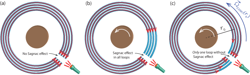
Figure 4: Apparatus for physically distinguishing between the static Levi-Civita metric and the Lewis metrics of the Weyl class, based on the Sagnac effect: a set (“coil”) of optical fiber loops around the central cylinder, in which counterpropagating light beams are injected. (a) Levi-Civita static cylinder, coil at rest with respect to the distant stars: the Sagnac effect vanishes in every loop. (b) Rotating cylinder of the Weyl class, coil at rest with respect to the distant stars: a Sagnac effect arises in every loop. (c) Lewis cylinder of the Weyl class, coil rotating [with respect to the distant stars] with the angular velocity of the ZAMO at $r_{0}$: the Sagnac effect vanishes only for the loop of radius $r=r_{0}$; for $r>r_{0}$ ($<r_{0}$) the beams co-rotating (counter-rotating) with the cylinder take longer to complete the loop.

$$\Omega_{{\rm ZAMO}}(r)=-\frac{\mathcal{A}_{\bar{\phi}}e^{2\Phi}}{g_{\bar{\phi}\bar{\phi}}}=-\left[\frac{j}{1/4-\lambda_{{\rm m}}}-\frac{1/4-\lambda_{{\rm m}}}{j}\alpha^{2}r^{2(1-4\lambda_{{\rm m}})}\right]^{-1}\ .$$ (69)

Consider then a set (“coil”) of circular optical fiber loops concentric with the cylinder, as depicted in Fig. 4. For a static cylinder ($j=0$), and a coil at rest in the star-fixed coordinates of (61), the Sagnac effect vanishes in every loop. When the metric is given in a different coordinate system, rotating with respect to (61), a Sagnac effect arises in a coil at rest therein; such effect is however globally eliminated by simply spinning the coil with some angular velocity. For a rotating cylinder ($j\neq 0$), and a coil at rest in the coordinates of (61) [see Fig. 4(b)], a Sagnac effect arises in every loop, given by Eq. (68). Now, along one single loop of radius $r_{0}$ [Fig. 4 (c)], the effect can always be eliminated, by spinning the coil with an angular velocity equaling that of the ZAMO on site, $\Omega_{{\rm ZAMO}}(r_{0})$. However, due to the $r-$dependence of $\Omega_{{\rm ZAMO}}(r)$, in all other loops of radius $r\neq r_{0}$ a Sagnac effect arises. Hence, given a Lewis metric in an arbitrary coordinate system, a physical experiment to determine whether it corresponds to a static or rotating cylinder would be to consider a coil of concentric optical fiber loops, as illustrated in Fig. 4, and checking whether one can globally eliminate the Sagnac effect along the whole coil by spinning it with some angular velocity. This reflects the basic fact that, contrary to the case around a static cylinder, in the rotating case it is not possible to globally eliminate $\bm{\mathcal{A}}$ through any rigid rotation (in fact, through any globally valid coordinate transformation, cf. Secs. 5.2.3 and 5.3.4).

It is worth observing that, for $\lambda_{{\rm m}}<1/4$ (case of the range where circular geodesics are allowed, and the metric clearly represents the field of a cylindrical source, see Sec. 5.2.3), $\mathcal{A}_{\bar{\phi}}$ has opposite sign to $j$ [cf. Eq. (63)], and so, by Eq. (68), for loops fixed with respect to the distant stars, it is the light beams propagating in the sense opposite to the cylinder’s rotation that take longer to complete the loop. Moreover, for spacelike $\partial_{\bar{\phi}}$ (i.e., $g_{\bar{\phi}\bar{\phi}}>0$), $\Omega_{{\rm ZAMO}}(r)$ has the same sign of $j$, so that the ZAMOs rotate (with respect to the distant stars) in the same sense as the cylinder. Both effects are thus in agreement with the intuitive notion that the cylinder’s rotation “drags” the “local spacetime geometry” with it, and consequently with the physical interpretation in Sec. 2.2.1.

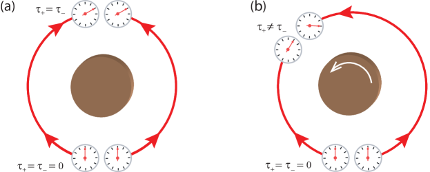
Figure 5: Apparatus for distinguishing between the field of static and rotating cylinders, based on the observer invariant gravitomagnetic clock effect: a pair of clocks in oppositely rotating circular geodesics. (a) In the static case, both clocks measure the same proper time between the events where they meet, $\tau_{+}=\tau_{-}$; (b) in the rotating case, the proper times differ, $\tau_{+}>\tau_{-}$.

Finally, we notice that in the limit $\lambda_{{\rm m}}=0$, corresponding to cosmic strings (Sec. 5.2.4), the Sagnac effect subsists, and so all the above applies for the distinction between the fields of spinning and non-spinning strings.

Gravitomagnetic clock effect

Another effect that allows to distinguish between the fields of static and rotating Weyl class cylinders is the gravitomagnetic clock effect. As seen in Sec. 5.2.3, the difference in orbital periods for pairs of particles in oppositely rotating geodesics, as measured in the star-fixed coordinate system of (61), reduces to the Sagnac time delay. Hence, one could replace the optical fiber loops in Fig. 4 by pairs of particles in geodesic motion, with analogous results: in the case of the static cylinder, the effect globally vanishes, the periods of circular geodesics being independent of their rotation sense. In the case of the rotating cylinder, the geodesics co-rotating with the cylinder have shorter periods than the counter-rotating ones. (Notice that this is opposite to the situation in the Kerr spacetime, cf. e.g. [71, 114]; that is down to the dominance therein of the second term of (29), which vanishes herein). It is possible, by a transformation to a rotating frame, to eliminate the delay for orbits of a given radius $r_{0}$; but it is not possible to do so globally, i.e. for all $r$. It is possible, however, to physically distinguish between the two metrics using only one pair of particles, through the observer invariant two-clock effect discussed in Sec. 3.1: consider a pair of clocks in oppositely rotating circular geodesics, as illustrated in Fig. 5. For the Levi-Civita static cylinder ($j=0$), the proper time measured between the events where they meet is the same for both clocks ($\Delta\tau=0$). For the rotating cylinder, by contrast, the proper times measured by each clock between meeting events differ ($\Delta\tau\neq 0$), being longer for the co-rotating clock: $\tau_{+}>\tau_{-}$. Their values are computed from Eqs (28), (31), (32), using the metric components in (61) [or, equivalently, in (37)-(38), since the effect does not depend on the reference frame].

5.3.2 Local vs global staticity

According to the usual definition in the literature (e.g. [115, 116, 32, 7, 6, 79, 117]), a spacetime is static iff it admits a hypersurface-orthogonal timelike Killing vector field $\xi^{\alpha}$. The hypersurface orthogonal condition amounts to demanding its dual 1-form $\xi_{\alpha}$ to be locally [6] of the form

$$\xi_{\alpha}=\eta\partial_{\alpha}\psi\ ,$$ (70)

where $\eta$ and $\psi$ are two smooth functions. This condition is equivalent to the vanishing of the vorticity (12) of the integral curves of $\xi^{\alpha}$. One can show [116] that if this condition is satisfied then a coordinate system can be found in which the metric takes a diagonal form. In such coordinates, the hypersurfaces orthogonal to $\xi^{\alpha}$ are the level surfaces of the time coordinate [7]. This is, however, a local notion, since such coordinates may not be globally satisfactory [7, 8] (as exemplified in Sec. 5.3.4 below).

A distinction should thus be made between local and global staticity. Notions of global staticity have been put forth in different, but equivalent formulations, by Stachel [6] and Bonnor [7], both amounting to demanding (70) to hold globally in the region under consideration, for some (single valued) function $\psi$. In [6], an enlightening formulation is devised, in terms of the 1-form $\bm{\chi}$ “inverse” to $\xi^{\alpha}$, defined by $\chi_{\alpha}\propto\xi_{\alpha}$ and $\chi_{\alpha}\xi^{\alpha}=1\Rightarrow\chi_{\alpha}\equiv\xi_{\alpha}/\xi^{2}$: it is noted that the condition that (70) is locally obeyed is equivalent to $\bm{\chi}$ being closed, $\mathbf{d}\bm{\chi}=0$, in which case $\xi^{\alpha}$ is dubbed a locally static Killing vector field; and that the condition that (70) holds globally amounts to demanding $\bm{\chi}$ to be moreover exact, i.e., $\bm{\chi}=\mathbf{d}\psi$ ($\Leftrightarrow\chi_{\alpha}=\partial_{\alpha}\psi$), for some some global function $\psi$. In this case $\xi^{\alpha}$ is dubbed globally static. A spacetime is then classified as locally static iff it admits a locally static time-like Killing vector field $\xi^{\alpha}$, and globally static iff it admits a globally static $\xi^{\alpha}$.

Consider now a stationary metric in the form (1). For the time-like Killing vector field $\xi^{\alpha}=\partial_{t}^{\alpha}$, we have $\bm{\chi}=\mathbf{d}t-\bm{\mathcal{A}}$; thus, the condition for $\xi^{\alpha}$ being locally static reduces to $\mathbf{d}\bm{\mathcal{A}}=0$, i.e., to the spatial 1-form $\bm{{\rm\mathcal{A}}}$ being closed; and it being globally static amounts to $\bm{\mathcal{A}}$ being exact. It follows that

Proposition 5.1

A spacetime is locally static iff it is possible to find a coordinate system where the metric takes the form (1) with $\mathbf{d}\bm{\mathcal{A}}=0$. The spacetime is globally static if $\bm{{\rm\mathcal{A}}}$ is moreover exact, i.e, if $\bm{{\rm\mathcal{A}}}=\mathbf{d}\varphi$, for some globally defined (single valued) function $\varphi$.

In the case of axistationary metrics, Eq. (4), $\bm{\mathcal{A}}=\mathcal{A}_{\phi}\mathbf{d\phi}$ with $\mathcal{A}_{\phi}$ independent of $\phi$, so the closedness condition $0=\mathbf{d}\bm{\mathcal{A}}=\mathbf{d}\mathcal{A}_{\phi}\wedge\mathbf{d\phi}$ amounts to $\mathcal{A}_{\phi}=constant$ [118], and the exactness condition to $\bm{{\rm\mathcal{A}}}=0$, since $\oint_{C}\mathbf{d}\phi\neq 0$ for any closed loop $C$ enclosing the axis $r=0$.

The Levi-Civita static metric (46) is clearly locally and globally static, since $\bm{{\rm\mathcal{A}}}=0$ therein. The Lewis metric of the Weyl class, as its canonical form (61) reveals, is an example of a metric which is locally but not globally static.

We propose yet another equivalent definition of global staticity, based on the hypersurfaces $\Sigma$ orthogonal to the Killing vector field $\xi^{\alpha}$, which proves enlightening in this context. Such hypersurfaces are the level surfaces $\psi=const.$ of the function $\psi(t,r,\phi,z)$ in Eq. (70). Choosing, without loss of generality, coordinates such that $\xi^{\alpha}=\partial_{t}^{\alpha}$, it follows that $\partial_{\alpha}\psi=\chi_{\alpha}=g_{0\alpha}/g_{00}$, i.e., by (1),

$$\mathbf{d}\psi=\mathbf{d}t-\mathcal{A}_{i}\mathbf{d}x^{i}\ \Leftrightarrow\ \psi=t-f(x^{i})\ ,$$

with $\mathbf{d}f=\mathcal{A}_{i}\mathbf{d}x^{i}$. Thus, $\psi$ is a (single-valued) function iff that is true for $f(x^{i})$, which amounts to the level surfaces $t=f(x^{i})+const$ ($\Leftrightarrow\psi=const.$) intersecting each integral line of $\partial_{t}$ exactly once. Such hypersurfaces are time slices. One can then say that a spacetime is globally static iff it admits a hypersurface orthogonal Killing vector field, whose hypersurfaces intersect each worldline of the congruence exactly once. Now, by definition, locally these hypersurfaces consist of the events that are simultaneous with respect to the laboratory observers (2) (whose worldlines are tangent to $\partial_{t}$); if they intersect each worldline of the congruence exactly once, they are global simultaneity hypersurfaces. (This is immediately seen by defining a new time coordinate $t^{\prime}=\psi$, which is constant along the hypersurfaces $\Sigma$ orthogonal to $\partial_{t^{\prime}}=\partial_{t}$). Hence,

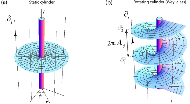
Figure 6: $t,r,\phi$ plot of the hypersurfaces orthogonal to the Killing vector field $\partial_{t}$ in: (a) the Levi-Civita static metric; (b) the canonical form (61) of the Lewis metric for a Weyl class rotating cylinder. The redundant $z$ coordinate has been suppressed, and the bar in $\bar{\phi}$ in Eq. (61) omitted. In (a) $\partial_{t}$ is orthogonal to hypersurfaces of global simultaneity (the planes $t=const.$), signaling that the spacetime is globally static. In (b) the orthogonal hypersurfaces are helicoids, described by $t-\mathcal{A}_{\phi}\phi=const.$, which are not hypersurfaces of global simultaneity, intersecting each integral curve of $\partial_{t}$ infinitely many times. The spacetime is thus locally, but not globally static. Each $2\pi$ turn along $\phi$ leads to a different event in time; the jump between turns is the synchronization gap $2\pi\mathcal{A}_{\phi}$.

Proposition 5.2

A spacetime is locally static iff it admits a hypersurface orthogonal Killing vector $\xi^{\alpha}$; it is moreover globally static iff such hypersurfaces are of global simultaneity, i.e, if they intersect each integral line of $\xi^{\alpha}$ exactly once.

In Fig. 6, the hypersurfaces orthogonal to the Killing field $\partial_{t}$ in the Levi-Civita metric (46) and in the canonical form (61) for Lewis-Weyl metric are plotted, in a 3-D chart $\{t,r,\phi\}$ that omits the $z$ coordinate [and the bar in $\bar{\phi}$ in Eq. (61)]. In the former these are the planes $t=const.$, which are hypersurfaces of global simultaneity, along which all clocks can be synchronized. For the rotating Lewis-Weyl metric such hypersurfaces are helicoids, described by $t-\mathcal{A}_{\bar{\phi}}\bar{\phi}=const.$, which intersect each integral curve of $\partial_{t}$ infinitely many times, signaling that the spacetime is not globally static. Each $2\pi$ turn in the $\bar{\phi}$ coordinate does not lead back to the same event $\mathscr{P}_{1}$, but to another ($\mathscr{P}_{2}$) at a different coordinate time ($\Delta t=2\pi\mathcal{A}_{\bar{\phi}}$), hence they are clearly not global simultaneity hypersurfaces. Consequently, a global clock synchronization between the hypersurface orthogonal Killing observers is not possible in the Lewis-Weyl rotating metric. In other words, observers at rest with respect to the distant stars can globally synchronize their clocks in the Levi-Civita, but not in the Lewis-Weyl rotating metric. This is another physical difference, to be added to those discussed in Sec. 5.3.1.

The global non-staticity of the Lewis-Weyl metric can also be seen from the fact that the hypersurfaces $\psi=t-\mathcal{A}_{\bar{\phi}}\bar{\phi}=const.$ form a foliation whose space of leaves is the circle rather than the real line; in other words, leaves given by $\psi=2n\pi\mathcal{A}_{\bar{\phi}}$ coincide for integer $n$, implying that $\psi$ is not single valued. Indeed, $\psi$ is a function only locally, for $\bar{\phi}\in[0,2\pi[$; otherwise it takes multiple values for the same point: $\psi(t,r,\bar{\phi},z)\neq\psi(t,r,\bar{\phi}+2n\pi,z)$.

The locally static and globally stationary character of the Lewis-Weyl metric is thus transparent in the canonical form (61) [though not in the usual form (37)-(38)], and it is physically manifest in the setups in Figs. 4 (b)-(c) and 5 (b). The setups in Figs. 4-5 are also examples that Stachel’s criteria for global staticity is well posed and sound on physical grounds.

5.3.3 Global staticity and holonomy

A stationary spacetime is a principal bundle over the space manifold $\Sigma$, since this manifold is simply the quotient of the spacetime by the integral lines of the time-like Killing vector field $\xi^{\alpha}$, that is, by the $\mathbb{R}$-action corresponding to the flow of $\xi^{\alpha}$ [119, 120]. A local trivialization of this bundle is simply a choice of a time coordinate $t$ such that $\partial_{t}^{\alpha}=\xi^{\alpha}$, and the structure group is the additive group $(\mathbb{R},+)$. Choosing instead the parameterization $s=e^{t}$ changes sums to products and allows us to see the stationary spacetime as a principal bundle with the more familiar multiplicative structure group $(\mathbb{R}^{+},\cdot)=GL^{+}(1,\mathbb{R})$. The distribution of hyperplanes orthogonal to $\xi^{\alpha}$ defines a connection on this bundle, whose parallel transport corresponds to the synchronization of the clocks carried by the observers tangent to $\xi^{\alpha}$, using the Einstein procedure [10, 121]. Indeed, the synchronization equation along some curve $x^{i}(\lambda)$, which amounts to the condition that the curve be orthogonal (at every point) to $\xi^{\alpha}$, reads

$$\frac{dt}{d\lambda}-\mathcal{A}_{i}\frac{dx^{i}}{d\lambda}=0\quad\Leftrightarrow\quad\frac{ds}{d\lambda}-\mathcal{A}_{i}\frac{dx^{i}}{d\lambda}s=0\ ,$$ (71)

and so the connection 1-form is $\bm{\mathcal{A}}$. The curvature 2-form is therefore $\bm{\mathcal{F}}=\mathbf{d}\bm{\mathcal{A}}$, and so (cf. Sec. 5.3.2) the condition for $\xi^{\alpha}$ to be hypersurface orthogonal is that this connection be flat.

To compute the holonomy of this connection along a closed curve $C$ on $\Sigma$ we integrate Eq. (71) along the curve:

$$\frac{1}{s}\frac{ds}{d\lambda}=\mathcal{A}_{i}\frac{dx^{i}}{d\lambda}\quad\Leftrightarrow\quad\ln\left(\frac{s_{{\rm final}}}{s_{{\rm initial}}}\right)=\oint_{C}\mathcal{A}_{i}dx^{i}\ .$$ (72)

Therefore the initial and final values of $s$ under parallel transport along $C$ are related by

$$s_{{\rm final}}={\rm Hol}(C)\,s_{{\rm initial}}\ ,$$ (73)

where the holonomy of the connection along $C$, ${\rm Hol}(C)$, is the group element

$${\rm Hol}(C)=e^{\oint_{C}\mathcal{A}_{i}dx^{i}}\in\mathbb{R}^{+}.$$ (74)

If the connection is flat then the holonomy depends only on the homotopy class of $C$, that is, it is invariant under continuous deformations of $C$. Moreover, the holonomy is trivial, that is, ${\rm Hol}(C)=1$ for all closed curves $C$, if and only if $\oint_{C}\bm{\mathcal{A}}=0$ for all closed curves $C$, i.e., if and only if $\bm{\mathcal{A}}$ is exact. It follows from Sec. 5.3.2 that the local staticity of a spacetime is equivalent to the existence of a time-like Killing vector field $\xi^{\alpha}$ whose synchronization connection is flat (i.e., a hypersurface orthogonal $\xi^{\alpha}$), and global staticity to it having moreover a trivial holonomy. Hence, another way of phrasing the distinction between the Levi-Civita (46) and the rotating Weyl class metrics (61) is that in the former, but not in the latter, the hypersurface orthogonal Killing observers have a synchronization connection with trivial holonomy.

5.3.4 Geometrical distinction

It is well known (e.g. [3]) that the transformation

$$t^{\prime}=(t+b\phi)\ ;\qquad\phi^{\prime}=\frac{n-bc}{n}\left[\phi-\Omega t\right]\ ;\qquad\Omega=\frac{c}{n-bc}$$ (75)

puts the Weyl class Lewis metric (37)-(38) into a form similar to the Levi-Civita line element (46), with $\{t^{\prime},\phi^{\prime}\}$ in the place of $\{t,\phi\}$. Hence, locally, they are isometric (i.e., locally indistinguishable). On the other hand, it is also known that this transformation is not globally satisfactory [7, 8], and that the two solutions globally differ, which is sometimes (inaccurately) assigned to topological differences. Their distinction, from a mathematical point of view, is indeed a subtle and not so well understood issue in the literature. It is however a realization of the mathematical relationship between globally, and locally but non-globally static spacetimes established by Stachel [6], as we shall now show.

We start by observing that the topology of the underlying manifolds is in fact the same: $\mathbb{R}^{1}\times\mathbb{R}^{3}\backslash\{r=0\}$. Therefore, it must be at the level of the metric that the differences arise. Let us then dissect the nature of transformation (75). In what pertains to the angular coordinate, it consists of a rotation $\bar{\phi}=\phi-\Omega t$ with the angular velocity $\Omega$ that leads to the star-fixed coordinates $\{x^{\bar{\alpha}}\}$ of Eqs. (54)-(55), composed with the “re-scaling” $\phi^{\prime}=\bar{\phi}(n-bc)/n$, which accounts for the different angular deficits of the spatial metrics $h_{ij}$ [Eq. (4)] that occur when one identifies the parameter $a$ in Eq. (46) with that in (54)-(55). The latter step is actually not necessary [one can instead identify $a$ in (46) with $\alpha^{-1}$], which is clear from the canonical form (61) of the metric. The transformation can actually be much simplified starting from the latter, which is immediately diagonalized (since $\mathcal{A}_{\bar{\phi}}$ is constant) through the transformation

$$t^{\prime}=t-\mathcal{A}_{\bar{\phi}}\bar{\phi}\equiv t-\frac{j}{\lambda_{{\rm m}}-1/4}\bar{\phi}\ ;\qquad\phi^{\prime}=\bar{\phi}\ ,$$ (76)

leading to

$$ds^{2}=-\frac{r^{4\lambda_{{\rm m}}}}{\alpha}dt^{\prime 2}+r^{4\lambda_{{\rm m}}(2\lambda_{{\rm m}}-1)}(dr^{2}+dz^{2})+\alpha r^{2(1-2\lambda_{{\rm m}})}d\phi^{\prime 2}\ ,$$ (77)

which is locally the Levi-Civita line element. One may check [substituting, in (76), $\bar{\phi}=\phi-\Omega t$] that it diagonalizes the original form (37)-(38) of the metric as well, yielding (77). Transformation (76) amounts to redefining the time coordinate so that it is constant along the hypersurfaces orthogonal to the Killing vector field $\partial_{t}$, plotted in Fig. 6 (b). That is, $t^{\prime}$ is the function $\psi$ as defined in Sec. 5.3.2 above. Since, in the original coordinates in (61), $\bar{\phi}$ is a periodic coordinate, with the identification $(t,\bar{\phi})=(t,\bar{\phi}+2\pi)$, transformation (76) leads to a coordinate system where the events $(t^{\prime},\phi^{\prime})$ and $(t^{\prime}-2\pi\mathcal{A}_{\bar{\phi}},\,\phi^{\prime}+2\pi)$ are identified, and neither $\phi^{\prime}$ or $t^{\prime}$ are periodic. In the Levi-Civita static metric, however, the periodic quantity is the angular coordinate [$\phi$, in the notation in (46)], which is a requirement of the matching to the interior solution [94]. Therefore, to effectively convert the metric (61) into the Levi-Civita metric, one must, in addition to the coordinate transformation (76), discard the original identifications and force instead, in (77), $\phi^{\prime}$ to be periodic, through the identification $(t^{\prime},\phi^{\prime})=(t^{\prime},\,\phi^{\prime}+2\pi)$. Such prescription, however, is not a global diffeomorphism. Namely, the map is neither injective nor single-valued: for instance, events $\mathscr{P}_{1}$: $(t,\bar{\phi})=(0,\bar{\phi}_{1})$ and $\mathscr{P}_{2}$: $(t,\bar{\phi})=(2\pi\mathcal{A}_{\bar{\phi}},\,\bar{\phi}_{1}+2\pi)$ in Fig. 6, which are distinct in the original manifold, would be mapped into the same event $(t^{\prime},\phi^{\prime})=(-\mathcal{A}_{\bar{\phi}}\bar{\phi}_{1},\,\bar{\phi}_{1})=(-\mathcal{A}_{\bar{\phi}}\bar{\phi}_{1},\,\bar{\phi}_{1}+2\pi)$ in the static solution; conversely, the ordered pairs $\mathscr{P}{}_{3}$: $(t,\bar{\phi})=(0,0)$ and $\mathscr{P}{}_{4}$: $(t,\bar{\phi})=(0,2\pi)$, which yield the same event in the original manifold, would be mapped into the two distinct events $\mathscr{P}^{\prime}_{3}$: $(t^{\prime},\phi^{\prime})=(0,0)$ and $\mathscr{P}^{\prime}_{4}$: $(t^{\prime},\phi^{\prime})=(-2\pi\mathcal{A}_{\bar{\phi}},\,2\pi)$ in the static solution. Only locally is the map bijective. Since only through such a map is it possible to obtain one from the other, that means that no global identification between the two metrics exists, thus they are not globally isometric.

It is worth noting that, in spite of the fact that the underlying manifolds are topologically indistinguishable, topology still plays an important role in the relationship between the exterior field of static and rotating cylinders of the Weyl class, in that, as explained in Sec. 2.3, it is the cylindrical “hole” along the axis $r=0$ that allows the existence of closed but non exact forms, i.e., curl-free forms $\bm{\mathcal{\sigma}}$ with non-vanishing circulation $\oint_{C}\bm{\mathcal{\sigma}}$ along closed loops $C$. Now, when a local but non-global diffeomorphism, such as the prescription above, exists between two manifolds, a closed but non-exact 1-form in one manifold can be mapped into an exact one in the other manifold [6]. On the other hand, as discussed in Sec. 5.3.2, global staticity consists of the exact character of the 1-form $\bm{\chi}$, inverse to the hypersurface orthogonal time-like Killing vector field ($\partial_{t}$, in this case). Consequently, globally static and locally but non-globally static metrics, connected by local diffeomorphisms, can coexist on such underlying topology. This is precisely the situation between the rotating and static Lewis metrics of the Weyl class: the 1-form inverse to the Killing vector field $\partial_{t}$ on the metric (61), $\bm{\chi}=\mathbf{d}t-\bm{\mathcal{A}}$, which is not exact (manifesting the global non-staticity of $\partial_{t}$), is mapped, via (76), into the exact 1-form $\mathbf{d}t^{\prime}$, inverse of the globally static Killing vector field $\partial_{t^{\prime}}$, on the target manifold [the Levi-Civita spacetime, described by (77) under the identification $(t^{\prime},\phi^{\prime})=(t^{\prime},\,\phi^{\prime}+2\pi)$, with $t^{\prime}$ assumed a single valued function].

5.4 Matching to the van Stockum cylinder

It was shown by van Stockum [81] that the Lewis metric has a smooth matching with the interior solution corresponding to an infinite, rigidly rotating cylinder of dust. In order to address the matching problem, we first establish the connection between the Lewis metric and van Stockum’s form for the exterior solution. The latter can be written as [122]

$$ds_{*}^{2}=-Fdt_{*}^{2}+2Mdt_{*}d\phi+\mathcal{H}(dr_{*}^{2}+dz_{*}^{2})+Ld\phi^{2}\ ,$$ (78)

with

$$F = \frac{(2N-1)(r_{*}/R)^{2N+1}+(2N+1)(r_{*}/R)^{1-2N}}{4N}\ ;$$ (79)

$$M = wR^{2}\frac{(2N+1)(r_{*}/R)^{2N+1}+(2N-1)(r_{*}/R)^{1-2N}}{4N}\ ;$$ (80)

$$L = R^{2}\frac{(2N+1)^{3}(r_{*}/R)^{2N+1}+(2N-1)^{3}(r_{*}/R)^{1-2N}}{16N}\ ;$$ (81)

$$\mathcal{H} = e^{-w^{2}R^{2}}(r_{*}/R)^{-2w^{2}R^{2}};\qquad\ N=\sqrt{1/4-w^{2}R^{2}}\ .$$ (82)

There are thus only two independent, positive parameters $w$ and $R$, the latter being the cylinder’s radius. The line element $ds_{*}$ in Eqs. (78)-(82), as well as the coordinates $t_{*}$, $r_{*}$, $z_{*}$, have the (usual) dimensions of length; this contrasts with the usual Lewis line element in (37)-(38), where $ds$ is dimensionless, and written in terms of dimensionless coordinates $t$, $r$ and $z$. Hence, in order to compare the two, we must first write, for the Lewis metric, a line element in the form $ds_{*}^{2}=\mathcal{R}^{2}ds^{2}$, where $\mathcal{R}$ is a constant with dimensions of length. Through the parameter redefinition $a=a_{*}\mathcal{R}^{1-n}$, $b=b_{*}/\mathcal{R}$, $c=\mathcal{R}c_{*}$, this line element becomes

$$ds_{*}^{2}=-f(r_{*})dt_{*}^{2}+2k(r_{*})dt_{*}d\phi+\left[\frac{r_{*}}{\mathcal{R}}\right]^{(n^{2}-1)/2}(dr_{*}^{2}+dz_{*}^{2})+l(r_{*})d\phi^{2}\ ,$$ (83)

where $(t_{*},r_{*},z_{*})\equiv(\mathcal{R}t,\mathcal{R}r,\mathcal{R}z)$ are coordinates with dimensions of length, $f(r_{*})\equiv f(r_{*},a_{*},c_{*},n)$, $k(r_{*})\equiv k(r_{*},a_{*},b_{*},c_{*},n)$, and $l(r_{*})\equiv l(r_{*},a_{*},b_{*},c_{*},n)$. By comparing the expressions for $g_{r_{*}r_{*}}$, and matching terms with the same powers in $r_{*}$ in the remainder of the metric components, we find that the metric (78)-(82) follows from (83) and (38) through the substitutions

$$\mathcal{R} = R/\sqrt{e}\ ;\qquad n\ =\ 2N\ ;\qquad a_{*}\ =\ \frac{2N+1}{4N}R^{2N-1}\ ;$$ (84)

$$b_{*} = \frac{1-2N}{1+2N}wR^{2}\ ;\qquad c_{*}=-\frac{\sqrt{1-4N^{2}}}{2R}=-w\ .$$ (85)

Notice that parameters $n$, $a_{*}$, $b_{*}$, $c_{*}$ are real iff $wR<1/2$; hence the van Stockum cylinder belongs to the Weyl class for $wR<1/2$, and to the Lewis class for $wR>1/2$. The metric can be put in the form (4), with

$$e^{2\Phi}=F\ ;\qquad\mathcal{A}_{\phi}=\frac{M}{F}\ ;\qquad h_{rr}=h_{zz}=\mathcal{H};\qquad h_{\phi\phi}=r_{*}^{2}e^{-2\Phi}\ .$$ (86)

The corresponding gravitoelectric and gravitomagnetic fields are

$$\vec{G}=\frac{2w^{2}Re^{w^{2}R^{2}}\left[(r_{*}/R)^{4N}-1\right](r_{*}/R)^{2w^{2}R^{2}-1}}{2N+1+(r/R)^{4N}(2N-1)};\qquad\ \vec{H}=\frac{8wNe^{w^{2}R^{2}}(r_{*}/R)^{2N-1+2w^{2}R^{2}}}{2N+1+(r_{*}/R)^{4N}(2N-1)}.$$ (87)

Observe that $\vec{G}=0$ for $r_{*}=R$; by virtue of (18), this means that a test particle dropped from rest therein remains at rest (i.e., particles at rest are geodesic). Again, this hints at the fact that the metric is written in a rotating coordinate system, the centrifugal inertial force exactly canceling out the gravitational attraction. Observe moreover that $g_{00}$ becomes positive (i.e., the Killing vector $\partial_{t_{*}}$ ceases to be time-like) for $r_{*}^{4N}>R^{4N}(2N+1)/(1-2N)$, which, as discussed in Sec. 5.2 (see also Sec. 4.2), is typical of a rotating frame.

5.4.1 Interior solution

The interior solution is given by Eq. (78), with [81, 122]

$$F=1;\qquad M=wr_{*}^{2};\qquad L=r_{*}^{2}-w^{2}r_{*}^{4};\qquad\mathcal{H}=e^{-w^{2}r_{*}^{2}}\ ,$$ (88)

depending on the single parameter $w$. It can be put in the form (4), with

$$\Phi=0;\qquad\mathcal{A}_{\phi}=wr_{*}^{2};\qquad h_{r_{*}r_{*}}=h_{z_{*}z_{*}}=e^{-w^{2}r_{*}^{2}};\qquad h_{\phi\phi}=r_{*}^{2}\ .$$ (89)

The corresponding gravitoelectric and gravitomagnetic fields are

$$\vec{G}=0\ ;\qquad\ \vec{H}=2we^{w^{2}r_{*}^{2}}\partial_{z_{*}}\ ,$$ (90)

and the gravitomagnetic tidal tensor as measured by the rest observers has the only non-vanishing components $\mathbb{H}_{rz}=\mathbb{H}_{zr}=-w^{3}r_{*}$. Thus $\mathbb{H}_{\alpha\beta}$ is symmetric; since $\mathbb{H}_{[\alpha\beta]}=-4\pi\epsilon_{\alpha\beta\mu\nu}J^{\mu}u^{\nu}$ [52], where $J^{\mu}\equiv-T^{\mu\sigma}u_{\sigma}$ is the mass-energy current as measured by the rest observers of 4-velocity $u^{\alpha}$, this means that no spatial mass currents [$h_{\ \nu}^{\mu}J^{\nu}$, see Eq. (3)] are measured by $u^{\alpha}$, i.e., the metric is written in a coordinate system co-rotating with the dust, cf. [81]. Observe moreover that $\vec{G}=0$ everywhere inside the cylinder; this is just the condition that the circular motion of the dust particles is solely driven by gravity (i.e., geodesic), so in the dust rest frame a centrifugal inertial force arises that exactly balances the gravitational attraction.

Let $\sigma^{(3)}$ be a stationary 3-D hypersurface which is the common boundary of two stationary spacetimes, and $\sigma$ the projected 2-D surface on the corresponding space manifolds $\Sigma$, as defined in Sec. 2. Let $\vec{n}$ be the unit vector normal to $\sigma$. The matching of the two solutions along $\sigma^{(3)}$ amounts to matching the induced metric on $\sigma^{(3)}$, $g_{\alpha\beta}|_{\sigma^{(3)}}$, plus the extrinsic curvature of $\sigma^{(3)}$. In the GEM formalism, and when $\sigma$ is connected, this is guaranteed (see [14] and footnote 3 therein) by the continuity across $\sigma$ of the GEM fields $\vec{G}$ and $\vec{H}$, gravitomagnetic potential 1-form $\bm{\mathcal{A}}$ (up to an exact form $\mathbf{d}f$, for some function $f$ on $\sigma$, corresponding to the freedom associated to the choice of $t$), spatial metric $h_{ij}$, and extrinsic curvature $K_{ij}\equiv\mathcal{L}_{n}h_{ij}$ of the spatial 2-surface $\sigma$:

$$\vec{G}_{{\rm int}}=\vec{G}_{{\rm ext}}\ ;\qquad\vec{H}_{{\rm int}}=\vec{H}_{{\rm ext}}\ ;\qquad\bm{\mathcal{A}}_{{\rm int}}=\bm{\mathcal{A}}_{{\rm ext}}+\mathbf{d}f\ ;$$

$$(h_{{\rm int}})_{ij}=(h_{{\rm ext}})_{ij}\ ;\qquad(K_{ij})_{{\rm int}}=(K_{ij})_{{\rm ext}}\ .$$

It follows from Eqs. (86)-(87) and (89)-(90) that these conditions (with $\bm{\mathcal{A}}_{{\rm int}}=\bm{\mathcal{A}}_{{\rm ext}}\Rightarrow\mathbf{d}f=0$) are satisfied across the cylinder’s surface $r_{*}=R$ with unit normal $\vec{n}=(h_{r_{*}r_{*}})^{-1/2}\vec{\partial}_{r_{*}}$, and so indeed the interior solution (88) smoothly matches the exterior (79)-(82). The rotation of coordinates that we noticed (Sec. 5.2) in the usual form of the Lewis-Weyl metric has thus a simple interpretation here: the coordinate system in (37)-(38) [or equivalently, in (78)-(82)], is rigidly co-rotating with the interior cylinder.

5.4.2 Matching in canonical form

We have seen in Sec. 5.2 that the star-fixed (“canonical”) coordinates for the Lewis metric of the Weyl class are obtained from the usual coordinates in (37)-(38) by the transformation (53), with $\Omega\equiv d\phi/dt$ one of the dimensionless angular velocities in (52) (depending on the sign of $a$). Since here $a_{*}>0$, cf. Eq. (84), the star-fixed coordinates for the Weyl class van Stockum exterior metric analogously follows by applying to (78)-(82) the transformation

$$\bar{\phi}=\phi-\Omega_{*}t_{*}\ ;\qquad\Omega_{*}\equiv\frac{d\phi}{dt_{*}}=\frac{\Omega}{\mathcal{R}}=\frac{c_{*}}{n-b_{*}c_{*}}=-\frac{4w}{(1+2N)^{2}}\ ,$$ (91)

where the angular velocity $\Omega_{*}$ now has the (usual) dimensions of inverse length, and, in the last equality, we substituted Eqs. (84)-(85). This yields the line element

$$ds^{2}=-\bar{F}dt_{*}^{2}+2\bar{M}dt_{*}d\bar{\phi}+\mathcal{H}(dr_{*}^{2}+dz_{*}^{2})+Ld\bar{\phi}^{2}\ ,$$ (92)

with $\mathcal{H}$ and $L$ given by Eqs. (81)-(82), and

$$\bar{F}=\frac{16N}{(1+2N)^{3}}\left[\frac{r_{*}}{R}\right]^{1-2N}\ ;\qquad\ \bar{M}=-\frac{R^{4}w^{3}}{2N}\bar{F}\ .$$ (93)

One can show, after some algebra, that (91) indeed corresponds to the transformation to the star-fixed coordinate system obtained in [81] [Eqs. (4.7) and (10.16) therein], and Eqs. (92)-(93) to the exterior metric as written in such coordinate system [Eqs. (10.17) therein, apart from a typo in the expression for $F$, where an extra $2wR$ factor is present]. Observe that $g_{00}=-\bar{F}$ is now negative for all $r_{*}$, so that the Killing vector field $\partial_{t_{*}}$ is time-like everywhere, contrary to the situation in (78)-(82). The Komar mass and angular momentum per unit length for the metric (92)-(93) can be obtained by applying the integrals (57) to any tube of unity $z_{*}-$length enclosing the cylinder [or by substituting (84)-(85) in (58)-(60), recalling that $a=a_{*}\mathcal{R}^{1-n}$, $b=b_{*}/\mathcal{R}$, $c=\mathcal{R}c_{*}$, and observing that $j_{*}=j\mathcal{R}$]; they read, respectively,

$$\lambda_{{\rm m}}=\frac{1-2N}{4}=\frac{1-\sqrt{1-4w^{2}R^{2}}}{4}\ ;\qquad j_{*}=\frac{R^{4}w^{3}}{4}\ .$$ (94)

Notice that $j_{*}$ has the usual dimensions of length. The metric (92)-(93) can be written in a canonical form akin to that in Sec. 5.2.2. For that, we first observe that [similarly to the usual form of the Lewis metric (37)-(38)] the line element $ds$ in (61), as well as the coordinates $t$, $r$, $z$ therein, are dimensionless; hence we need to write, for the same metric, a line element $ds_{*}^{2}=\mathcal{R}^{2}ds^{2}$ with the dimensions of length:

$$ds_{*}^{2}=-\frac{r_{*}^{4\lambda_{{\rm m}}}}{\alpha_{*}}\left(dt_{*}-\frac{j_{*}}{\lambda_{{\rm m}}-1/4}d\bar{\phi}\right)^{2}+\left[\frac{r_{*}}{\mathcal{R}}\right]^{4\lambda_{{\rm m}}(2\lambda_{{\rm m}}-1)}(dr_{*}^{2}+dz_{*}^{2})+\alpha_{*}r_{*}^{2(1-2\lambda_{{\rm m}})}d\bar{\phi}^{2},$$ (95)

where $\alpha_{*}=\alpha\mathcal{R}^{4\lambda_{{\rm m}}}$, $\mathcal{R}$ is, again, a constant with dimensions of length, and $(t_{*},r_{*},z_{*})\equiv(\mathcal{R}t,\mathcal{R}r,\mathcal{R}z)$ are coordinates with dimensions of length. The canonical form of the van Stockum exterior solution then follows from using, in (95), $\lambda_{{\rm m}}$ and $j_{*}$ as given by (94), and

$$\alpha_{*}=\frac{R^{4\lambda_{{\rm m}}}(1-2\lambda_{{\rm m}})^{3}}{1-4\lambda_{{\rm m}}}\ ;\qquad\;\mathcal{R}=R/\sqrt{e}\ .$$ (96)

It naturally possesses all the “canonical” properties listed in Sec 5.2.2. In this special case, however, $\lambda_{{\rm m}}$, $j_{*}$, and $\alpha_{*}$ are not independent parameters, as is clear from Eqs. (94) and (96); the metric has only two independent parameters (which boil down to $R$ and $w$), just like in the original coordinate system in (78)-(82). It is also useful to write the metric in the form (4), with

$$e^{2\Phi} = \ \bar{F}\ =\alpha_{*}^{-1}R^{4\lambda_{{\rm m}}}(r_{*}/R)^{4\lambda_{{\rm m}}}\quad\Rightarrow\quad\Phi\ =\ 2\lambda_{{\rm m}}\ln(r_{*}/R)+const.\ ;$$ (97)

$$\mathcal{A}_{\bar{\phi}} = \frac{j_{*}}{\lambda_{{\rm m}}-1/4}=-\frac{R^{4}w^{3}}{2N}\ ;$$ (98)

$$h_{r_{*}r_{*}} = h_{z_{*}z_{*}}=\left[\frac{r_{*}}{R}e^{1/2}\right]^{4\lambda_{{\rm m}}(2\lambda_{{\rm m}}-1)};\qquad h_{\bar{\phi}\bar{\phi}}=r_{*}^{2}e^{-2\Phi}.$$ (99)

Since $\Omega_{*}$ in Eq. (91) is the angular velocity of the star-fixed frame with respect to a frame co-rotating with the interior cylinder, then the cylinder rotates with angular velocity $-\Omega_{*}$ with respect to the star-fixed frame (cf. [81]). Observe that $\Omega_{*}$ is negative; this means that the cylinder is rotating in the positive $\bar{\phi}$ direction. Observe moreover that $\mathcal{A}_{\bar{\phi}}$ is negative; this implies, via Eqs. (5) and (6), that the star-fixed “laboratory” observers have negative angular momentum, and that the zero angular momentum observers rotate in the same sense of the cylinder (i.e., are “dragged” around by the cylinder’s rotation), as occurs e.g. in the Kerr spacetime, and in agreement with an intuitive notion of frame-dragging. The GEM fields read

$$G_{i}=-\frac{2\lambda_{{\rm m}}}{r_{*}}\delta_{i}^{r}\ ;\qquad\ \vec{H}=0\ ,$$ (100)

the discussion of their physical effects in Sec. 5.2.3 applying herein.

The interior solution written in star-fixed coordinates is likewise obtained from (78), (88) (the metric written in coordinates comoving with the cylinder) by the transformation (91), yielding a metric of the form (92), with $\mathcal{H}$ and $L$ still given by Eqs. (88) and

$$\bar{F} = 1+4\frac{r_{*}^{4}}{R^{4}}\frac{\lambda_{{\rm m}}^{2}}{(1-2\lambda_{{\rm m}})^{2}}+2\frac{r_{*}^{2}}{R^{2}}\frac{\lambda_{{\rm m}}\left[2(1-2\lambda_{{\rm m}})^{2}-1\right]}{(1-2\lambda_{{\rm m}})^{3}}\ ;$$ (101)

$$\bar{M} = wr_{*}^{2}\frac{r_{*}^{2}w^{2}-4(1-\lambda_{{\rm m}})\lambda_{{\rm m}}}{(1-2\lambda_{{\rm m}})^{2}}\ .$$ (102)

Observe from Eqs. (101) and (94) that $\bar{F}$ depends only on the (dimensionless) quantities $r_{*}/R$ and $\lambda_{{\rm m}}$. Since $0<r_{*}<R$ within the cylinder, and $wR<1/2\Rightarrow 0<\lambda_{{\rm m}}<1/4$ for the Weyl class, it follows that $\bar{F}>0\Rightarrow g_{00}<0$ everywhere inside the cylinder, and so the Killing vector field field $\partial_{t_{*}}$ is everywhere time-like therein. Moreover, it follows from the expressions for $L$ and $\mathcal{H}$ in Eqs. (88) that the coordinate basis vectors $\partial_{r_{*}}$, $\partial_{\bar{\phi}}$, and $\partial_{z_{*}}$ are everywhere spacelike. This tells us that the coordinate system fixed to the distant stars is well defined everywhere within the cylinder. Writing the metric in the form (4) yields the GEM fields and spatial metric:

$$G_{i} = \frac{4\lambda_{{\rm m}}r_{*}\left[\lambda_{{\rm m}}-r_{*}^{2}w^{2}+\Delta(2\lambda_{{\rm m}}-1)w^{2}\right]}{r_{*}^{4}w^{2}-4\lambda_{{\rm m}}^{2}r_{*}^{2}+\Delta\left[r_{*}^{2}\left(2-4\lambda_{{\rm m}}\right)+\Delta(4\lambda_{{\rm m}}^{2}-4\lambda_{{\rm m}}+1)\right]w^{2}}\delta_{i}^{r_{*}}\ ;$$

$$\vec{H} = -\frac{2\Delta w^{3}e^{r_{*}^{2}w^{2}}(\Delta^{2}w^{2}+2r_{*}^{2}+2R^{2})}{(3r_{*}^{2}+R^{2})(1-4\lambda_{{\rm m}})+\Delta-2w^{2}(R^{4}-r_{*}^{4})-2\Delta^{3}w^{4}}\partial_{z_{*}}\ ;$$

$$h_{r_{*}r_{*}} = h_{z_{*}z_{*}}=e^{-w^{2}r_{*}^{2}}\ ;\qquad\ h_{\bar{\phi}\bar{\phi}}=r_{*}^{2}e^{-2\Phi}=\frac{r_{*}^{2}}{\bar{F}}\ ,$$

where $\Delta\equiv R^{2}-r_{*}^{2}$. At the cylinder’s surface $r_{*}=R$ ($\Rightarrow\Delta=0$), and so we have

$$(G_{{\rm int}})_{i}=(G_{{\rm ext}})_{i}=-\frac{2\lambda_{{\rm m}}}{R}\delta_{i}^{r_{*}}\ ;\qquad\ \vec{H}_{{\rm int}}=\vec{H}_{{\rm ext}}=0\ ;$$

$$(\mathcal{A}_{\phi})_{{\rm int}}=(\mathcal{A}_{\phi})_{{\rm ext}}=\frac{j_{*}}{\lambda_{{\rm m}}-1/4}\ ;\qquad\ (h_{{\rm int}})_{\bar{\phi}\bar{\phi}}=(h_{{\rm ext}})_{\bar{\phi}\bar{\phi}}=\alpha_{*}R^{2(1-2\lambda_{{\rm m}})}\ ;$$ (103)

$$(h_{{\rm int}})_{z_{*}z_{*}}=(h_{{\rm int}})_{r_{*}r_{*}}=(h_{{\rm ext}})_{z_{*}z_{*}}=(h_{{\rm ext}})_{r_{*}r_{*}}=e^{2\lambda_{{\rm m}}(2\lambda_{{\rm m}}-1)}\ .$$

The extrinsic curvature ($K_{ij}\equiv\mathcal{L}_{n}h_{ij}$) of that surface, with unit normal $\vec{n}=(h_{r_{*}r_{*}})^{-1/2}\vec{\partial}_{r_{*}}$, has non-vanishing components

$$(K_{{\rm int}})_{\bar{\phi}\bar{\phi}} = (K_{{\rm ext}})_{\bar{\phi}\bar{\phi}}=\frac{2R(1-2\lambda_{{\rm m}})^{4}}{1-4\lambda_{{\rm m}}}e^{\lambda_{{\rm m}}(1-2\lambda_{{\rm m}})}\ ;$$ (104)

$$(K_{{\rm int}})_{z_{*}z_{*}} = (K_{{\rm ext}})_{z_{*}z_{*}}=-\frac{4\lambda_{{\rm m}}(1-2\lambda_{{\rm m}})}{R}e^{-\lambda_{{\rm m}}(1-2\lambda_{{\rm m}})}\ .$$ (105)

Thus, indeed there is a smooth matching between the interior metric in star-fixed coordinates and the exterior metric in canonical (star-fixed) form. This is the expected result, for we knew that the matching is possible in the more usual coordinates employed in Sec. 5.4.1.

The Komar mass per unit length can be computed from the interior solution by using Eq. (15), $Q_{\xi}(\mathcal{V})=-K/(8\pi)\int_{\mathcal{V}}R_{\ \beta}^{\alpha}\xi^{\beta}n_{\alpha}d\mathcal{V}$, with $\mathcal{V}$ the cylinder of radius $r_{*}=R$ and unit $z_{*}-$length on the hypersurface $\Sigma_{t_{0}}$ of constant time $t_{*}=t_{0}$, $n_{\alpha}=-(1-w^{2}r_{*}^{2})^{-1/2}\nabla_{\alpha}t_{*}$ the unit covector normal to $\Sigma_{t_{0}}$, $\xi^{\alpha}=\partial_{t_{*}}^{\alpha}$, $d\mathcal{V}=\sqrt{g_{\Sigma}}dr_{*}d\bar{\phi}dz_{*}$, where $g_{\Sigma}=e^{-2w^{2}r_{*}^{2}}(r_{*}^{2}-w^{2}r_{*}^{4})$ is the determinant of the metric induced on $\Sigma_{t_{0}}$, and (again) $K=-2$. It yields, as expected, the same result (94) obtained from the exterior solution. The same is true for the angular momentum per unit length $j_{*}$.

5.5 The Lewis class

When $n$ is imaginary, the structure of the curvature invariants, Eqs. (39)-(41) and (50), is the following:

$$\star\!\mathbf{R}\cdot\mathbf{R}=0;\qquad\mathbf{R}\cdot\mathbf{R}\geq 0\ \ (<0)\ \ {\rm for}\ \ |n|\leq\sqrt{3}\ \ (>\sqrt{3});\qquad\mathbb{M}<0\ \mbox{(real)}\ .$$

These conditions mean that there are no observers, at any point, for which $\mathbb{H}_{\alpha\beta}=0$ [91, 33, 79]. This in turn implies, via Eq. (25), that $\vec{H}$ cannot vanish in any coordinate system where the metric is time-independent. Therefore the metric possesses (locally and globally) intrinsic gravitomagnetic tidal tensor $\mathbb{H}_{\alpha\beta}$ and globally intrinsic gravitomagnetic field $\vec{H}$, in the classification scheme of [33]. Since $\vec{H}$ is proportional to the vorticity of the observer congruence [$\vec{H}=2\vec{\omega}$, cf. Eq. (20)], this amounts to saying that hypersurface orthogonal time-like Killing vector fields do not exist. Hence, contrary to the Weyl class case, the metric is not locally static (as is well known, e.g. [80]). Thus these are fundamentally very different gravitational fields.

The fact that $\vec{H}\neq 0$ in any coordinate system where the metric is time-independent implies, e.g., that radial geodesics are not possible, and gyroscopes (with $\vec{S}\nparallel\vec{H}$) will always be seen to precess therein, cf. Eq. (21). The fact that $\mathbb{H}_{\alpha\beta}\neq 0$ for all observers means that spinning bodies in this spacetime are always acted by a force (23).

6 Conclusion

In this work we investigated the exterior gravitational fields produced by infinite cylinders, described by the Lewis metrics, focusing on a class of them — the Weyl class — whose metrics are known to be locally static, and to encompass the field of both static (the Levi-Civita solution) and rotating cylinders. We aimed at establishing the distinction between the two cases, both in terms of the physical effects and of the geometrical properties where the rotation imprints itself. We started by observing that gravitomagnetism has three levels (corresponding to three different orders of differentiation of $\vec{\mathcal{A}}$), described by the three mathematical objects: the gravitomagnetic vector potential $\vec{\mathcal{A}}$, the gravitomagnetic field $\vec{H}$, and the gravitomagnetic tidal tensor $\mathbb{H}_{\alpha\beta}$. Then we unveiled a hitherto unnoticed feature of the Weyl class metric: that by a simple coordinate rotation it can be put into an especially simple form, where (by contrast with the usual form in the literature) the Killing vector field $\partial_{t}$ is time-like everywhere, and the associated coordinate system is fixed to the distant stars. In such a reference frame both $\vec{H}$ and $\mathbb{H}_{\alpha\beta}$ vanish everywhere, the vector $\vec{\mathcal{A}}$ being the only surviving gravitomagnetic object, which, in the case of a rotating cylinder, cannot be made to vanish by any global coordinate transformation. This perfectly mirrors the electromagnetic analogue (Sec. 4): in the exterior of an infinitely long rotating charged cylinder both the magnetic field $\vec{B}=\nabla\times\vec{A}$ and the magnetic tidal tensor $B_{\alpha\beta}$ vanish, just like for a static cylinder; only the magnetic vector potential $\vec{A}$ is non-vanishing. (Reinforcing the analogy, the gravitoelectric potential $\Phi$ in these coordinates also remarkably matches its electromagnetic counterpart, if we identify charge with mass.) The resulting metric, moreover, depends only on three parameters: the Komar mass and angular momentum per unit length, plus the angle deficit. We argue this to be the canonical form of the Lewis metrics of the Weyl class. It makes explicit, for the Weyl class, and in terms of parameters with a clear physical meaning, the earlier finding in [4] that there are only three independent parameters in the Lewis metric. It also makes explicit that the exterior metric of a rotating cylinder formally differs from that of a static one only by the presence of a non-vanishing, but irrotational $\vec{\mathcal{A}}$ (i.e., of a closed 1-form $\bm{\mathcal{A}}$). By contrast with classical electrodynamics, where a vector potential with vanishing curl $\nabla\times\vec{A}=\vec{B}=0$ is pure gauge, but similarly to quantum electrodynamics, where it manifests itself in the Aharonov-Bohm effect (Sec. 4.1), the gravitomagnetic vector potential $\vec{\mathcal{A}}$ does manifest itself physically, in effects involving loops around the central cylinder, namely in the Sagnac effect, clock synchronization, and the gravitomagnetic clock effect. The Sagnac effect, in particular, is seen to be described exactly by an equation formally analogous to the Aharonov-Bohm effect in the exterior of an infinitely long rotating charged cylinder (or of a long solenoid). This substantiates, with a concrete result, earlier suggestions in the literature: the suggestion in [3] that the Lewis metrics possess some topological analogue of the Aharonov-Bohm effect (by showing what it is); and the claim in [23, 6, 109, 110, 108, 100] that the Sagnac effect can be seen as a gravitational analogue of the Aharonov-Bohm effect (by revealing a one to one correspondence using the gravitational setup that is physically analogous to the Aharonov-Bohm electromagnetic setting [78]).

The physical effects mentioned above are global, in that they arise only on paths $C$ enclosing the central cylinder. The gravitomagnetic clock effect is naturally so, as it is defined for circular orbits. The Sagnac effect and synchronization gap, both given by the circulation of the gravitomagnetic potential 1-form, $\oint_{C}\bm{\mathcal{A}}$, vanish (in the canonical, star-fixed frame) along any loop not enclosing the cylinder, and have the same value along any loop enclosing it, regardless of its shape. Global effects are seen to actually be the only physical differences between the metrics, since all local and quasi-local dynamical fields (i.e., tidal and inertial fields, respectively) are shown to be the same as for the static cylinder.

The difference between metrics of rotating and static Weyl class cylinders turns out to be an archetype of the distinction between globally static, and locally static but globally stationary spacetimes. We reformulated the Stachel-Bonnor notions of local and global staticity into equivalent, more enlightening forms in this context, by showing that: (i) local staticity amounts to existence of a coordinate system (1) where the gravitomagnetic potential 1-form $\bm{\mathcal{A}}$ is closed, and global staticity to it being moreover exact; (ii) equivalently, while local staticity amounts to the existence of a hypersurface orthogonal Killing time-like vector field, global staticity amounts to such hypersurface being moreover a global simultaneity hypersurface. This distinction can moreover be formulated in terms of a connection that describes the clock synchronization for observers tangent to $\xi^{\alpha}$, local staticity amounting to such connection being flat, and global staticity to its holonomy being trivial. We also dissected the nature of the well known transformation that takes the Weyl class metric into the static Levi-Civita one, showing it not to be a global diffeomorphism (thus not a globally valid coordinate transformation), and the two metrics to be locally, but not globally isometric, in spite of the underlying manifolds sharing same topology.

The distinction above, both on physical and geometrical grounds, was made transparent by writing the Weyl class metrics in their “canonical” form, based on star-fixed coordinates, which therefore play a key role in this work. In the “real world” such reference frame is physically set up by pointing telescopes at the distant stars, and used in various experiments (including the detection of gravitomagnetic effects, such as gyroscope and orbital precessions [28, 63]). It should be noted, however, that the underlying physical distinction between the two fields is not an artifact, nor does it rely on the use of any particular frame. In fact, in Sec. 5.3.1 we propose (thought) physical apparatuses — namely a coil of optical loops, and the observer independent gravitomagnetic clock effect — that are frame independent.

References

References

- [1] T. Lewis, “Some special solutions to the equations of axially symmetric gravitational fields,” Proc. Roy. Soc. Lond. A136 (1932) 179–192.
- [2] K. Bronnikov, N. O. Santos, and A. Wang, “Cylindrical Systems in General Relativity,” Class. Quant. Grav. 37 no. 11, (2020) 113002, arXiv:1901.06561.
- [3] M. F. A. da Silva, L. Herrera, F. M. Paiva, and N. O. Santos, “The parameters of the Lewis metric for the Weyl class,” General Relativity and Gravitation 27 no. 8, (Aug, 1995) 859–872.
- [4] M. A. H. MacCallum and N. O. Santos, “Stationary and static cylindrically symmetric Einstein spaces of the Lewis form,” Classical and Quantum Gravity 15 no. 6, (1998) 1627.
- [5] J. B. Griffiths and J. Podolsky, Exact Space-Times in Einstein’s General Relativity. Cambridge Monographs on Mathematical Physics. Cambridge University Press, Cambridge, 2009.
- [6] J. Stachel, “Globally stationary but locally static space-times: A gravitational analog of the Aharonov-Bohm effect,” Phys. Rev. D26 (1982) 1281–1290.
- [7] W. B. Bonnor, “The rigidly rotating relativistic dust cylinder,” Journal of Physics A: Mathematical and General 13 (1980) 2121.
- [8] F. J. Tipler, “Rotating cylinders and the possibility of global causality violation,” Phys. Rev. D9 (1974) 2203–2206.
- [9] L. Herrera and N. O. Santos, “Geodesics in Lewis space-time,” Journal of Mathematical Physics 39 no. 7, (1998) 3817–3827.
- [10] L. D. Landau and E. M. Lifshitz, The classical theory of fields; 4rd ed., vol. 2 of Course of theoretical physics. Butterworth-Heinemann, Oxford, UK, 1975. Trans. from the Russian.
- [11] C. Cattaneo, “General relativity: Relative standard mass, momentum, energy and gravitational field in a general system of reference,” Il Nuovo Cimento (1955-1965) 10 no. 2, (1958) 318–337.
- [12] R. T. Jantzen, P. Carini, and D. Bini, “The Many faces of gravitoelectromagnetism,” Annals Phys. 215 (1992) 1–50, arXiv:gr-qc/0106043.
- [13] D. Lynden-Bell and M. Nouri-Zonoz, “Classical monopoles: Newton, nut space, gravomagnetic lensing, and atomic spectra,” Rev. Mod. Phys. 70 (Apr, 1998) 427–445.
- [14] F. C. Mena and J. Natário, “Matching stationary spacetimes,” J. Geom. Phys. 59 (2009) 448–458, arXiv:0802.2615.
- [15] R. Gharechahi, J. Koohbor, and M. Nouri-Zonoz, “General relativistic analogs of Poisson’s equation and gravitational binding energy,” Phys. Rev. D 99 (2019) 084046.
- [16] C. W. Misner, K. S. Thorne, and J. A. Wheeler, Gravitation. W. H. Freeman, San Francisco, 1973.
- [17] O. Semerák, “Circular orbits in stationary axisymmetric spacetimes,” General Relativity and Gravitation 30 no. 8, (Aug, 1998) 1203–1215.
- [18] B. R. Iyer and C. V. Vishveshwara, “Frenet-Serret description of gyroscopic precession,” Phys. Rev. D 48 (Dec, 1993) 5706–5720.
- [19] G. Sagnac, “L’éther lumineux démontré par l’effet du vent relatif d’éther dans un interféromètre en rotation uniforme,” C. R. Acad. Sci., Paris 157 (1913) 708–710.
- [20] G. Sagnac, “Sur la preuve de la réalité de l’éther lumineux par l’expérience de l’interférographe tournant,” C. R. Acad. Sci., Paris 157 (1913) 1410–1413.
- [21] M. v. Laue, “Zum Versuch von F. Harress,” Annalen der Physik 367 no. 13, (1920) 448–463.
- [22] E. J. Post, “Sagnac effect,” Rev. Mod. Phys. 39 (Apr, 1967) 475–493.
- [23] A. Ashtekar and A. Magnon, “The Sagnac effect in general relativity,” J. Math. Phys. 16 (1975) 341–344.
- [24] W. W. Chow, J. Gea-Banacloche, L. M. Pedrotti, V. E. Sanders, W. Schleich, and M. O. Scully, “The ring laser gyro,” Rev. Mod. Phys. 57 (Jan, 1985) 61–104.
- [25] E. Kajari, M. Buser, C. Feiler, and W. P. Schleich, “Rotation in relativity and the propagation of light,” Riv. Nuovo Cim. 32 (2009) 339–438, arXiv:0905.0765.
- [26] A. Tartaglia, “General relativistic corrections to the Sagnac effect,” Phys. Rev. D58 (1998) 064009, arXiv:gr-qc/9806019.
- [27] E. Kajari, R. Walser, W. P. Schleich, and A. Delgado, “Sagnac effect of Godel’s universe,” Gen. Rel. Grav. 36 (2004) 2289, arXiv:gr-qc/0404032.
- [28] I. Ciufolini and J. A. Wheeler, Gravitation and Inertia. Princeton Series in Physics, Princeton, NJ, 1995.
- [29] E. Massa and C. Zordan, “Relative kinematics in general relativity the Thomas and Fokker precessions,” Meccanica 10 no. 1, (Mar, 1975) 27–31.
- [30] W. Rindler and V. Perlick, “Rotating coordinates as tools for calculating circular geodesics and gyroscopic precession,” General Relativity and Gravitation 22 (1990) 1067–1081.
- [31] L. F. O. Costa and J. Natário, “Gravito-electromagnetic analogies,” General Relativity and Gravitation 46 no. 10, (2014) 1792, arXiv:1207.0465 [gr-qc].
- [32] S. W. Hawking and G. F. R. Ellis, The Large Scale Structure of Space-Time. Cambridge Monographs on Mathematical Physics. Cambridge University Press, 1973.
- [33] L. F. O. Costa, L. Wylleman, and J. Natário, “Gravitomagnetism and the significance of the curvature scalar invariants,” arXiv:1603.03143.
- [34] R. M. Wald, General Relativity. The University of Chicago Press, Chicago, 1984.
- [35] P. K. Townsend, “Black holes: Lecture notes,” arXiv:gr-qc/9707012.
- [36] R. O. Hansen and J. Winicour, “Killing inequalities for relativistically rotating fluids,” Journal of Mathematical Physics 16 (1975) 804–808.
- [37] A. Komar, “Covariant conservation laws in general relativity,” Phys. Rev. 113 (1959) 934–936.
- [38] J. Natário, “Mathematical Relativity,” arXiv:2003.02855.
- [39] E. T. Whittaker, “On Gauss’ Theorem and the Concept of Mass in General Relativity,” Proceedings of the Royal Society of London Series A 149 (1935) 384–395.
- [40] J. Natário, “Quasi-Maxwell interpretation of the spin–curvature coupling,” General Relativity and Gravitation 39 no. 9, (Sep, 2007) 1477–1487.
- [41] D. Kay, Tensor Calculus. Schaum’s Outline Series. McGraw-Hill Companies,Incorporated, 1988.
- [42] L. F. Costa and J. Natário, “The Coriolis field,” Am. J. Phys. 84 (2016) 388, arXiv:1511.02458.
- [43] M. Nouri-Zonoz and A. Parvizi, “Gaussian curvature and global effects: Gravitational Aharonov-Bohm effect revisited,” Phys. Rev. D88 no. 2, (2013) 023004, arXiv:1306.1883.
- [44] E. Massa, “Space tensors in general relativity ii: Physical applications,” General Relativity and Gravitation 5 (1974) 573–591.
- [45] M. Mathisson, “Neue mechanik materieller systemes,” Acta Phys. Polon. 6 (1937) 163. [Gen. Relativ. Gravit. 42, 1011 (2010)].
- [46] A. Papapetrou, “Spinning test particles in general relativity. 1.,” Proc. Roy. Soc. Lond. A209 (1951) 248–258.
- [47] W. G. Dixon, “Dynamics of extended bodies in general relativity. I. Momentum and angular momentum,” Proc. Roy. Soc. Lond. A314 (1970) 499–527.
- [48] W. G. Dixon, “A covariant multipole formalism for extended test bodies in general relativity,” Il Nuovo Cimento 34 (1964) 317.
- [49] S. E. Gralla, A. I. Harte, and R. M. Wald, “Bobbing and Kicks in Electromagnetism and Gravity,” Phys. Rev. D81 (2010) 104012, arXiv:1004.0679 [gr-qc].
- [50] L. F. O. Costa, J. Natário, and M. Zilhão, “Spacetime dynamics of spinning particles: Exact electromagnetic analogies,” Phys. Rev. D93 no. 10, (2016) 104006, arXiv:1207.0470 [gr-qc].
- [51] F. A. E. Pirani, “On the physical significance of the Riemann tensor,” Acta Phys. Polon. 15 (1956) 389–405. [Gen. Relativ. Gravit. 41,1215 (2009)].
- [52] L. Filipe Costa and C. A. R. Herdeiro, “Gravitoelectromagnetic analogy based on tidal tensors,” Phys. Rev. D78 (2008) 024021.
- [53] N. Dadhich, “Electromagnetic duality in general relativity,” Gen. Rel. Grav. 32 (2000) 1009–1023, arXiv:gr-qc/9909067 [gr-qc].
- [54] R. Maartens and B. A. Bassett, “Gravito-electromagnetism,” Classical and Quantum Gravity 15 no. 3, (1998) 705. http://stacks.iop.org/0264-9381/15/i=3/a=018.
- [55] B. Mashhoon, F. W. Hehl, and D. S. Theiss, “On the Gravitational effects of rotating masses - The Thirring-Lense Papers,” Gen. Rel. Grav. 16 (1984) 711–750.
- [56] A. Einstein, letter to E. Mach, Zurich, 25 June 1913, see Reference [16], page 544 (Figure 21.5).
- [57] A. Einstein, The meaning of Relativity, 5th edition. Princeton University Press, Princeton, NJ, 1970.
- [58] L. I. Schiff, “Motion of a gyroscope according to Einstein’s theory of gravitation,” Proceedings of the National Academy of Sciences 46 no. 6, (1960) 871–882.
- [59] J. M. Cohen and D. R. Brill, “Further examples of ’machian’ effects of rotating bodies in general relativity,” Il Nuovo Cimento B (1965-1970) 56 (1968) 209–219.
- [60] L. Herrera, G. A. Gonzalez, L. A. Pachon, and J. A. Rueda, “Frame dragging, vorticity and electromagnetic fields in axially symmetric stationary spacetimes,” Class. Quant. Grav. 23 (2006) 2395–2408, arXiv:gr-qc/0602040.
- [61] L. Herrera, J. Carot, and A. Di Prisco, “Frame dragging and super-energy,” Phys. Rev. D76 (2007) 044012, arXiv:0707.0867.
- [62] I. Ciufolini and E. C. Pavlis, “A confirmation of the general relativistic prediction of the Lense-Thirring effect,” Nature 431 (2004) 958–960.
- [63] I. Ciufolini, “Dragging of inertial frames,” Nature 449 (2007) 41–47.
- [64] H. Elvang and P. Figueras, “Black saturn,” JHEP 2007 no. 05, (2007) 050.
- [65] P. Čížek and O. Semerák, “Perturbation of a Schwarzschild Black Hole Due to a Rotating Thin Disk,” The Astrophysical Journal Supplement Series 232 (2017) 14, arXiv:1710.07109.
- [66] J. M. Bardeen, W. H. Press, and S. A. Teukolsky, “Rotating Black Holes: Locally Nonrotating Frames, Energy Extraction, and Scalar Synchrotron Radiation,” The Astrophysical Journal 178 (1972) 347–370.
- [67] J. M. Bardeen, “A Variational Principle for Rotating Stars in General Relativity,” The Astrophysical Journal 162 (1970) 71.
- [68] O. Semerák, “What forces act in relativistic gyroscope precession?,” Classical and Quantum Gravity 13 (1996) 2987–2994.
- [69] J. M. Cohen and B. Mashhoon, “Standard clocks, interferometry, and gravitomagnetism,” Physics Letters A 181 (1993) 353 – 358.
- [70] W. B. Bonnor and B. R. Steadman, “The gravitomagnetic clock effect,” Classical and Quantum Gravity 16 no. 6, (1999) 1853.
- [71] D. Bini, R. T. Jantzen, and B. Mashhoon, “Gravitomagnetism and relative observer clock effects,” Class. Quant. Grav. 18 (2001) 653–670, arXiv:gr-qc/0012065.
- [72] R. Maartens, B. Mashhoon, and D. R. Matravers, “Holonomy and gravitomagnetism,” Class. Quant. Grav. 19 (2002) 195–202, arXiv:gr-qc/0104049.
- [73] B. Schutz, Gravity from the Ground Up: An Introductory Guide to Gravity and General Relativity. Cambridge University Press, 2003. See pp. 246-251.
- [74] R. P. Feynman, R. B. Leighton, and M. Sands, The Feynman Lectures on Physics, Vol. II. Addison Wesley, 1964. http://www.feynmanlectures.info/.
- [75] W. B. Bonnor and B. R. Steadman, “The gravitomagnetic clock effect,” Classical and Quantum Gravity 16 (1999) 1853–1861.
- [76] B. Mashhoon and N. O. Santos, “Rotating cylindrical systems and gravitomagnetism,” Annalen der Physik 9 no. 1, (2000) 49–63.
- [77] A. Tartaglia, “Detection of the gravitomagnetic clock effect,” Class. Quant. Grav. 17 (2000) 783–792, arXiv:gr-qc/9909006.
- [78] Y. Aharonov and D. Bohm, “Significance of electromagnetic potentials in the quantum theory,” Phys. Rev. 115 (Aug, 1959) 485–491.
- [79] H. Stephani, D. Kramer, M. A. H. MacCallum, C. Hoenselaers, and E. Herlt, Exact solutions of Einstein’s field equations. Cambridge University Press, 2004.
- [80] M. F. A. da Silva, L. Herrera, F. M. Paiva, and N. O. Santos, “On the parameters of Lewis metric for the Lewis class,” Class. Quant. Grav. 12 (1995) 111–118, arXiv:gr-qc/9607057.
- [81] W. J. van Stockum, “IX. The Gravitational Field of a Distribution of Particles Rotating about an Axis of Symmetry,” Proceedings of the Royal Society of Edinburgh 57 (1938) 135–154.
- [82] T. Levi-Civita, “Republication of: Einsteinian ds2 in newtonian fields. ix: The analog of the logarithmic potential,” General Relativity and Gravitation 43 no. 8, (2011) 2321–2330.
- [83] M. A. H. MacCallum, “Editorial note to: T. Levi-Civita, The physical reality of some normal spaces of Bianchi and to: Einsteinian ds2 in Newtonian fields. IX: The analog of the logarithmic potential,” General Relativity and Gravitation 43 no. 8, (2011) 2297–2306.
- [84] W. B. Bonnor, “Physical interpretation of vacuum solutions of Einstein’s equations. Part I. Time-independent solutions,” General Relativity and Gravitation 24 no. 5, (1992) 551–574.
- [85] R. Gautreau and R. B. Hoffman, “Exact solutions of the einstein vacuum field equations in weyl co-ordinates,” Nuovo Cimento B 61 (1969) 411–424.
- [86] W. B. Bonnor and M. A. P. Martins, “The interpretation of some static vacuum metrics,” Classical and Quantum Gravity 8 no. 4, (Apr, 1991) 727–738.
- [87] M. F. A. da Silva, L. Herrera, F. M. Paiva, and N. O. Santos, “The levi-civita space-time,” Journal of Mathematical Physics 36 no. 7, (1995) 3625–3631.
- [88] W. B. Bonnor and W. Davidson, “Interpreting the levi-civita vacuum metric,” Classical and Quantum Gravity 9 no. 9, (Sep, 1992) 2065–2068.
- [89] W. B. Bonnor, The Static Cylinder in General Relativity, pp. 113–119. Springer New York, New York, NY, 1999.
- [90] T. G. Philbin, “Perfect-fluid cylinders and walls – sources for the levi-civita spacetime,” Classical and Quantum Gravity 13 no. 5, (1996) 1217–1232.
- [91] C. B. G. McIntosh, R. Arianrhod, S. T. Wade, and C. Hoenselaers, “Electric and magnetic Weyl tensors: classification and analysis,” Classical and Quantum Gravity 11 (Jun, 1994) 1555–1564.
- [92] L. Wylleman and N. Van den Bergh, “Complete classification of purely magnetic, nonrotating, nonaccelerating perfect fluids,” Phys. Rev. D 74 (2006) 084001.
- [93] L. Herrera and N. O. Santos, “On the gravitomagnetic effects in cylindrically symmetric space-times,” J. Math. Phys. 42 (2001) 4956–4962, arXiv:gr-qc/0107040.
- [94] W. B. Bonnor, “Solution of Einstein’s equations for a line-mass of perfect fluid,” Journal of Physics A: Mathematical and General 12 no. 6, (1979) 847–851.
- [95] W. Israel, “Line sources in general relativity,” Phys. Rev. D 15 (Feb, 1977) 935–941.
- [96] L. Marder, “Gravitational Waves in General Relativity. I. Cylindrical Waves,” Proceedings of the Royal Society of London Series A 244 (1958) 524–537.
- [97] A. Z. Wang, M. F. A. da Silva, and N. O. Santos, “On parameters of the Levi-Civita solution,” Classical and Quantum Gravity 14 no. 8, (1997) 2417–2423.
- [98] O. Semerák, “Extremally accelerated observers in stationary axisymmetric spacetimes,” General Relativity and Gravitation 28 (Sep, 1996) 1151–1155.
- [99] O. Semerák, “Gravitomagnetic clock effect and extremely accelerated observers,” Classical and Quantum Gravity 16 no. 11, (1999) 3769–3770.
- [100] A. Barros, V. B. Bezerra, and C. Romero, “Global aspects of gravitomagnetism,” Mod. Phys. Lett. A18 (2003) 2673–2679, arXiv:gr-qc/0307062.
- [101] B. Jensen and H. H. Soleng, “General-relativistic model of a spinning cosmic string,” Phys. Rev. D 45 (May, 1992) 3528–3533.
- [102] V. Bezerra, “Some remarks on loop variables, holonomy transformation, and gravitational Aharonov-Bohm effect,” Annals Phys. 203 (1990) 392–409.
- [103] F. C. Mena, J. Natário, and P. Tod, “Avoiding closed timelike curves with a collapsing rotating null dust shell,” Class. Quant. Grav. 25 (2008) 045016, arXiv:0710.4696.
- [104] B. Linet, “The Static Metrics with Cylindrical Symmetry Describing a Model of Cosmic Strings,” Gen. Rel. Grav. 17 (1985) 1109–1115.
- [105] M. Hindmarsh and T. Kibble, “Cosmic strings,” Rept. Prog. Phys. 58 (1995) 477–562, arXiv:hep-ph/9411342.
- [106] L. H. Ford and A. Vilenkin, “A gravitational analogue of the Aharonov-Bohm effect,” Journal of Physics A: Mathematical and General 14 (1981) 2353–2357.
- [107] J. S. Dowker, “A gravitational Aharonov-Bohm effect,” Il Nuovo Cimento B (1965-1970) 52 (1967) 129–135.
- [108] M. L. Ruggiero, “The Sagnac effect in curved space-times from an analogy with the Aharonov-Bohm effect,” Gen. Rel. Grav. 37 (2005) 1845–1855, arXiv:gr-qc/0510047.
- [109] G. Rizzi and M. L. Ruggiero, “The Sagnac phase shift suggested by the Aharonov-Bohm effect for relativistic matter beams,” Gen. Rel. Grav. 35 (2003) 1745–1760, arXiv:gr-qc/0305046.
- [110] G. Rizzi and M. L. Ruggiero, “The Relativistic Sagnac effect: Two derivations,” arXiv:gr-qc/0305084.
- [111] M. L. Ruggiero and A. Tartaglia, “A Note on the Sagnac Effect and Current Terrestrial Experiments,” Eur. Phys. J. Plus 129 (2014) 126, arXiv:1403.6341 [gr-qc].
- [112] M. L. Ruggiero and A. Tartaglia, “A note on the Sagnac effect for matter beams,” The European Physical Journal Plus 130 no. 5, (May, 2015) 90.
- [113] J. Podolsky, R. Steinbauer, and R. Svarc, “Gyratonic pp-waves and their impulsive limit,” Phys. Rev. D90 no. 4, (2014) 044050, arXiv:1406.3227.
- [114] A. Tartaglia, “Geometric treatment of the gravitomagnetic clock effect,” General Relativity and Gravitation 32 no. 9, (Sep, 2000) 1745–1756.
- [115] A. Barnes, “Static perfect fluids in general relativity,” Journal of Physics A: General Physics 5 (1972) 374–393.
- [116] J. Ehlers and W. Kundt, Gravitation: an Introduction to current research, ed. L. Witten. Wiley, New York, 1962.
- [117] L. Wylleman and D. Beke, “Expanding perfect fluid generalizations of the C-metric,” Phys. Rev. D81 (2010) 104038, arXiv:1001.5263.
- [118] N. V. den Bergh and P. Wils, “A class of stationary Einstein-Maxwell solutions with cylindrical symmetry,” Journal of Physics A: Mathematical and General 16 no. 16, (1983) 3843–3851.
- [119] S. Harris, “Conformally stationary spacetimes,” Classical and Quantum Gravity 9 no. 7, (1992) 1823–1827.
- [120] M. T. Anderson, “On stationary vacuum solutions to the Einstein equations,” Annales Henri Poincare 1 (2000) 977, arXiv:gr-qc/0001091.
- [121] S. Bazański, “Is the geodesic hypothesis in general relativity falsifiable?,” Banach Center Publications 41 (1997) 273–285.
- [122] W. B. Bonnor, “The magnetic Weyl tensor and the van Stockum solution,” Classical and Quantum Gravity 12 no. 6, (1995) 1483.