Two-soliton molecule bouncing in a dipolar Bose-Einstein condensates under the effect of gravity

Abstract

The dynamics of a two-soliton molecule bouncing on the reflecting atomic mirror under the effect of gravity has been studied by analytical and numerical methods. The analytical description is based on the variational approximation. In numerical simulations, we observe the resonance oscillations of the two-soliton’s center-of-mass position and width, induced by modulated atomic mirror. Theoretical predictions are verified by numerical simulations of the nonlocal Gross-Pitaevskii equation (GPE) and qualitative agreement between them is found. Hamiltonian dynamic system for a dipolar Bose-Einstein condensates (BECs) has been studied.

(xxxxxxxxxx)

1 Introduction

Bose-Einstein condensates (BECs) were first realized in 1995 on vapors of rubidium,[1] sodium,[2] and lithium.[3] To observe quantum phenomenon such as Bose-Einstein condensate, the temperature must be of order $10^{-7}$ K. The phenomenon of Bose-Einstein condensation was predicted in 1925 by Einstein.[4] Bose introduced a method to derive the black-body spectrum for photon gas.[5] Einstein considered a gas of bosonic atoms, and concluded that, below a critical temperature, a large fraction of the atoms condenses in the lowest quantum state.[4]

The spin-polarized hydrogen has been a good candidate for BEC in the late 1970s and early 1980s. Using the quantum theory of corresponding states, Hecht[6] and Stwalley and Nosanow[7] concluded that spin-polarized hydrogen had no bounds states and would remain gaseous down to zero temperature and should be a good candidate to realize Bose-Einstein condensation in a dilute atomic gas. Many aspects of studies of spin-polarized hydrogen indicated that atomic systems can remain in a metastable gaseous state close to Bose-Einstein condensation conditions. Bose-Einstein condensation of atomic hydrogen was realized in 1998 by Kleppner, Greytak and collaborators.[8] Finally, Bose-Einstein condensation of photons in an optical microcavity was first realized in 2010 by Klaers and Weitz.[9]

An important progress has been made in the experimental cooling of trapped polar molecules that have a large magnetic moment.[10] In symmetrical molecules (such as $\mathrm{H_{2},\,O_{2},\,N_{2}}$), the centers of gravity of the positive and negative charges coincide in the absence of an external electric field. Such molecules have no intrinsic dipole moment and are called nonpolar. In asymmetrical molecules (such as $\mathrm{CO,\,OH,\,NH_{3},\,HCl,\,CaH,\,LiCs}$), the centers of gravity of the charges of opposite signs are displaced relative to each other. In this case, the molecules have an intrinsic dipole moment and are called polar.[10] Under the action of an external electric field, the charges in a nonpolar molecule become displaced relative to one another, the positive ones in the direction of the field, the negative ones against the field. As a result, the molecule acquires a dipole moment whose magnitude, as shown by experiments, is proportional to the field strength.[11]

As expected, the process of polarization of a nonpolar molecule proceeds as if the positive and negative charges of the molecule were bound to one another by elastic forces. The action of an external field on a polar molecule consists mainly in tending to rotate the molecule so that its dipole moment is arranged in the direction of the field. An external field does not virtually affect the magnitude of a dipole moment. Consequently, a polar molecule behaves in an external field like a rigid dipole.[11]

An experimental review[10] describes the rapidly developing field of ultracold polar molecules. Molecules with translational temperatures between 1 and 1000 mK can be easily manipulated with electromagnetic fields and trapped. Experimentally cold molecules were created from cold bosonic atoms by magnetic Feshbach resonances.[10, 11] The experimental review[10] provides a rigorous description of the methods for cooling, and trapping polar molecules. Reference 12 experimentally considered the formation of ultracold LiCs polar molecules by a single photoassociation step beginning from laser cooled atoms.

The University of Rostock group’s paper by Mitschke et al.[13] presents a detailed experimental observation of temporal soliton molecules. The authors[13] note that this structure exists only in dispersion-managed fiber. They predicted a bound state of temporal solitons in optical fibers numerically. Mitschke’s group described the first experimental demonstration of the existence of temporal optical soliton molecules. In recent experiment[14] with ultracold polar molecules, full control over the internal states of ultracold ${}^{23}\mathrm{Na}\,^{87}\mathrm{Rb}$ polar molecules was obtained. The authors used the microwave spectroscopy to control the rotational and hyperfine states of ultracold ground state ${}^{23}\mathrm{Na}\,^{87}\mathrm{Rb}$ polar molecules, which were created by them.[14]

Some other atoms, such as chromium, erbium, europium and dysprosium, have a large magnetic moment of several Bohr magnetons in their ground state, and thus experience significant magnetic dipole-dipole interactions. Chromium,[15, 16] dysprosium[17] and erbium[18] were Bose-condensed. The principal difference of chromium condensates from the alkali atom condensates is that, chromium has a large permanent magnetic dipole moment of $6\,\mu_{\mathrm{B}}$, and a scattering length of about $100\,a_{0}$, where $\mu_{\mathrm{B}}$ and $a_{0}$ are the Bohr magneton and the Bohr radius.[19] This allows to observe a perturbative effect of the dipolar interactions on the expansion dynamics of the gas cloud.[20]

In recent years, quantum bouncer problem has attracted the attention of physicists.[21, 22, 23, 24] Gibbs introduced the concept “quantum bouncer”[25] for the particle. Quantum bouncer problem was extensively studied in many pedagogical articles[26, 27] and original research papers.[23, 24, 28] Gea-Banaloche[27] analytically considered quantum bouncer problem and studied the reflection of a quantum particle from a reflecting impenetrable atomic mirror. In a recent work,[23] static and dynamic properties of a weakly interacting BEC in the quasi one-dimensional (1D) gravito-optical surface trap were studied by analytical and numerical means.

The dynamics of bisolitonic matter-waves in a BEC that was subjected to an expulsive harmonic potential and a gravitational potential have been studied in Ref. 29. The authors were using a non-isospectral scattering transform method and exact expressions for the bright-matter -wave bisolitons, and consequently received solution in terms of double-lump envelopes. Some aspects of the paper[29] were experimentally predicted.[30, 31, 32]

The dynamics of a matter-wave soliton on a reflecting penetrable surface (atomic mirror) in a uniform gravitational field were investigated in a research paper.[21] In recent review,[22] the dynamics of an oscillon, videlicet, a soliton-like cluster of the BEC on an oscillating atomic mirror in a uniform gravitational field were studied.

The paper is organized as follows. In Sec. 2, we describe the mathematical model and introduce the nonlocal Gross-Pitaevskii equation (GPE). In Sec. 3, the variational approximation for the analytical treatment of the nonlinear model is developed and its predictions are compared to numerical simulations of the nonlocal GPE. Section 4 is devoted to exploring the small amplitude dynamics. In Sec. 5, we consider the dynamics of action-angle variables and illustrate the distinctive features of the nonlinear model. In Sec. 6, the variational approximation for the nonlocal GPE for stationary state has been developed and applied to low energy shape oscillations of the condensate. In concluding Sec. 7, we summarize our results.

2 Model Description and Governing Equation

The atomic density at the center of a Bose-Einstein condensed atomic cloud is usually $10^{13}-10^{15}\;\mathrm{cm^{-3}}$, which the molecular density in air at room temperature and normal atmospheric pressure is of order $10^{19}\;\mathrm{cm^{-3}}$. In contrast to that in liquids and solids the density of atoms is typically $10^{22}\;\mathrm{cm^{-3}}$. In atomic nuclei, the density of nucleons is about $10^{38}\;\mathrm{cm^{-3}}$.

In ultracold quantum gases, a new kind of interaction via long-range and anisotropic dipolar forces arises in addition to short-range and isotropic contact interactions. The potential of dipole-dipole interactions is[11]

$$U_{dd}(r)=\frac{C_{dd}}{4\pi}\frac{1-3\cos^{2}\phi}{r^{3}},$$ (1)

where $C_{dd}=\mu_{0}\mu^{2}$ is the coupling constant for atoms having a permanent magnetic dipole moment $\mu$ ($\mu_{0}$ is the permeability of vacuum), and $C_{dd}=d^{2}/\varepsilon_{0}$ for atoms having permanent electric dipole moment $d$ ($\varepsilon_{0}$ is the permittivity of vacuum). The angle $\phi$ lies between the direction of polarization and the relative position of the atoms.

The dynamics of a dipolar BEC in the mean-field approximation at zero temperature is governed by the three-dimensional (3D) nonlocal GPE:[11, 33, 34]

$$i\hbar\frac{\partial\Psi}{\partial t}=\Big{[}-\frac{\hbar^{2}}{2m}\Delta+U_{\rm{ext}}(\mathbf{r})+\frac{4\pi a_{s}\hbar^{2}}{m}|\Psi|^{2}+\int\limits_{-\infty}^{\infty}U_{dd}(\mathbf{r}-\mathbf{r}^{\prime})|\Psi(\mathbf{r}^{\prime},t)|^{2}d\mathbf{r}^{\prime}\Big{]}\Psi,$$ (2)

where $\Psi(\mathbf{r},t)$ is the wave function of the condensate, normalized to the number of atoms $N=\int\limits_{-\infty}^{\infty}|\Psi|^{2}d\mathbf{r}$, $m$ is the atomic mass, $a_{s}$ is the s-wave scattering length (below, we shall be concerned with an attractive BEC for which $a_{s}<0$), and

$$U_{\rm{ext}}(\mathbf{r})=\frac{m}{2}\big{[}\omega_{x}^{2}x^{2}+\omega_{\perp}^{2}(y^{2}+z^{2})\big{]}$$ (3)

is the axially symmetric trapping potential.

When the transverse confinement is strong enough, one can assume that the transverse dynamics are frozen, so that the dynamics are effectively in 1D. In this case, the wave function may be effectively factorized as $\Psi(\mathbf{r},t)=\psi(x,t)\varphi(y,z)$, where $\varphi(y,z)=\exp\big{[}-(y^{2}+z^{2})/(2a_{\perp}^{2})\big{]}/(\sqrt{\pi}a_{\perp})$ is the ground state of the 2D harmonic oscillator in the transverse direction, with $a_{\perp}=\sqrt{\hbar/m\omega_{\perp}}$ being the transverse harmonic oscillator length, $\omega_{\perp}$ is the transverse trap frequency. By substituting factorized expression into the 3D nonlocal GPE (2) and integration over the transverse variables $y$ and $z$, one derives the 1D nonlocal GPE:

$$i\hbar\frac{\partial\psi}{\partial t}=-\frac{\hbar^{2}}{2m}\frac{\partial^{2}\psi}{\partial x^{2}}+\Big{[}U_{\mathrm{ext}}(x)+2a_{s}\hbar\omega_{\perp}|\psi|^{2}+\int\limits_{-\infty}^{\infty}U_{dd}(|x-x^{\prime}|)|\psi(x^{\prime},t)|^{2}dx^{\prime}\Big{]}\psi.$$ (4)

The reduced 1D potential of the dipole-dipole interactions was derived by Sinha and Santos.[35] Thus, the $U_{dd}(x)$ is of the form

$$U_{dd}(x)=-\frac{2\rho d^{2}}{a_{\perp}^{3}}\Big{[}2|x|-\sqrt{\pi}(1+2x^{2})e^{x^{2}}\mathrm{erfc}(|x|)\Big{]},$$ (5)

where $d$ is the dipole moment, $\rho$ is a variable that may change between $\rho=1\>(\phi=0)$ and $\rho=-1/2\>(\phi=\pi/2)$. It is necessary to note that although the dipole-dipole interactions are long-ranged and divergent at the original 3D potential, i. e. $r=0$, the reduced 1D potential $U_{dd}(x)$ is regularized at $x=0$.

The BEC presents a giant matter-wave packet.[36, 37] Of special interest is the free fall of BEC above Earth’s surface. It is interesting to consider the motion of a matter-wave packet in a gravitational field over Earth s surface.[22, 38] In the present model, the gravitational field acts on atoms in the vertical direction and a horizontal atom mirror which reflects them back. The dancing matter-wave packet corresponds to a stationary state.

We now assume the axial parabolic trap to be the gravitational potential $mgx$ in its standard form, where $g$ is the acceleration of free fall and reflects gives potential $U(x)$. Rewrite Eq. (4) using the gravitational and reflecting potentials

$$i\hbar\frac{\partial\psi}{\partial t}=-\frac{\hbar^{2}}{2m}\frac{\partial^{2}\psi}{\partial x^{2}}+mgx\psi+U(x)\psi+\Big{[}2a_{s}\hbar\omega_{\perp}|\psi|^{2}+\int\limits_{-\infty}^{\infty}U_{dd}(|x-x^{\prime}|)|\psi(x^{\prime},t)|^{2}dx^{\prime}\Big{]}\psi.$$ (6)

For future analysis, rewrite Eq. (6) using the dimensionless variables: $x\rightarrow x/l_{g},\,t\rightarrow t/t_{g},\,l_{g}=(\hbar^{2}/(m^{2}g))^{1/3},\,t_{g}=(\hbar/(mg^{2}))^{1/3},\,V(x)=U(x)/(mgl_{g}),\,d\rightarrow d/\sqrt{mgl_{g}a_{\perp}^{3}}$, and the rescaled wave function $\psi\rightarrow\sqrt{2|a_{s}|\omega_{\perp}t_{g}}\psi$,

$$i\frac{\partial\psi}{\partial t}=-\frac{1}{2}\frac{\partial^{2}\psi}{\partial x^{2}}+kx\psi+V(x)\psi+q|\psi|^{2}\psi-2\rho d^{2}\psi\int\limits_{-\infty}^{\infty}R(|x-x^{\prime}|)|\psi(x^{\prime},t)|^{2}dx^{\prime},$$ (7)

where $R(x)\sim U_{dd}(x)$ is the dimensionless nonlocal kernel function. We introduced an additional dimensionless coefficient $k=\sin\chi$ to account for the possibility of altering the effect of gravity by changing the angle $\chi$ formed by the axis of the quasi 1D waveguide and the horizontal reflecting potential. For vertical position $\chi=\pi/2$ of the waveguide $k=1$, at smaller angles $0<\chi\leq\pi/2$, then $0<k\leq 1$. Another additional parameter $q$ is the dimensionless strength of attractive contact interactions $(q=1)$.

To estimate quantities of the model, we consider the ${}^{85}\mathrm{Rb}$ condensate, for which $a_{s}=-20\;\mathrm{nm},\,l_{g}\approx 1.3\;\mathrm{\mu m},\,t_{g}=0.36\;\mathrm{ms}$. The transversal frequency of radial confinement is $\omega_{\perp}=10^{3}\;\mathrm{rad/s}$. For the norm $N=4$, the soliton contains approximately 720 atoms. ${}^{7}\mathrm{Li}$ condensate with $a_{s}=-1.6\;\mathrm{nm}$ gives $l_{g}\approx 7\;\mathrm{\mu m},\,t_{g}=0.84\;\mathrm{ms},\,\omega_{\perp}=10^{4}\;\mathrm{rad/s}$ and the soliton contains approximately 1400 atoms.[21, 22]

3 The Variational Approximation

First of all, we develop the variational approximation for arbitrary forms of the reflecting potential $V(x)$ and gravitational potential.[39, 40] Equation (7) may be written in the form

$$i\psi_{t}=-\frac{1}{2}\psi_{xx}+kx\psi+V(x)\psi+q|\psi|^{2}\psi-\gamma\psi\int\limits_{-\infty}^{\infty}R(|x-x^{\prime}|)|\psi(x^{\prime},t)|^{2}dx^{\prime},$$ (8)

where $\gamma=2\rho d^{2}$ is the strength of dipole-dipole interactions and $\psi_{t}=\partial\psi/\partial t,\,\psi_{x}=\partial\psi/\partial x$.

The kernel function $R(x)$ is complicated for the variational analysis. In further calculations, we using the Gaussian response function[35, 41, 42]

$$R(x)=\frac{1}{\sqrt{2\pi}w}\exp{\Big{(}-\frac{x^{2}}{2w^{2}}\Big{)}},$$ (9)

which is normalized to one $\int\limits_{-\infty}^{\infty}R(x)dx=1$.

As a trial function for the two-soliton molecule, we use the first Gauss-Hermite function

$$\psi(x,t)=A(x-\xi)\exp\bigg{[}-\frac{(x-\xi)^{2}}{2a^{2}}+i\,b(x-\xi)^{2}+i\,v(x-\xi)+i\varphi\bigg{]},$$ (10)

where $A,\,a,\,\xi,\,v,\,b,\,\varphi$ are time dependent variational parameters, representing the two-soliton’s amplitude, width, center-of-mass position, velocity, chirp and phase.

It should be noted that comparison between numerical simulation of GPE and variational approximation used the Hermite-Gaussian and super-sech ansatzes is consequential in Ref. 43. The authors clearly established that the Hermite-Gaussian ansatz reproduces a bisoliton only for specific signs of some parameters in the Hermite-Gaussian ansatz. They also present special conditions where its ansatz strictly has the profile of bisoliton.[43] It should also be noted that in the classical paper of Lakoba and Kaup,[44] conditions for the Hermite-Gaussian ansatz are considered in order to obtain a quasi-two-soliton solution in the nonlinear Schr$\rm{\ddot{o}}$dinger equation.

The nonlocal GPE (8) can be obtained from the Lagrangian density

$${\cal L} = \frac{i}{2}\left(\psi\psi_{t}^{\ast}-\psi^{\ast}\psi_{t}\right)+\frac{1}{2}|\psi_{x}|^{2}+(kx+V(x))|\psi|^{2}+\frac{q}{2}|\psi|^{4}$$ (11)

$$- \frac{\gamma}{2}|\psi|^{2}\int\limits_{-\infty}^{\infty}R(|x-x^{\prime}|)|\psi(x^{\prime},t)|^{2}dx^{\prime}.$$

We assume that the reflecting potential $V(x)$ is represented by the Dirac delta function $V_{0}\delta(x)$, where $V_{0}$ is the strength of delta potential barrier.

Now, substituting the Gauss-Hermite function (10) and Gaussian response function (9) into Lagrangian density (11), one obtains

$${\cal L}_{1} = (x-\xi)^{2}\left[b_{t}(x-\xi)^{2}-2b(x-\xi)\xi_{t}+v_{t}(x-\xi)-v\xi_{t}+\varphi_{t}\right]$$ (12)

$$\times A^{2}e^{-(x-\xi)^{2}/a^{2}},$$

$${\cal L}_{2} = \left\{1-\frac{2(x-\xi)^{2}}{a^{2}}+(x-\xi)^{2}\left[\frac{(x-\xi)^{2}}{a^{4}}+(2b(x-\xi)+v)^{2}\right]\right\}$$ (13)

$$\times \frac{A^{2}}{2}e^{-(x-\xi)^{2}/a^{2}},$$

$${\cal L}_{3} = [k\,x+V_{0}\delta(x)]A^{2}(x-\xi)^{2}e^{-(x-\xi)^{2}/a^{2}},$$ (14)

$${\cal L}_{4} = \frac{qA^{4}}{2}(x-\xi)^{4}e^{-2(x-\xi)^{2}/a^{2}},$$ (15)

$${\cal L}_{5} = -\frac{\gamma A^{4}}{2\sqrt{2\pi}w}(x-\xi)^{2}e^{-(x-\xi)^{2}/a^{2}}\int\limits_{-\infty}^{\infty}e^{-(x-x^{\prime})^{2}/2w^{2}}(x^{\prime}-\xi)^{2}$$ (16)

$$\times e^{-(x^{\prime}-\xi)^{2}/a^{2}}dx^{\prime}.$$

To calculate the integral in ${\cal L}_{5}$, we make the change of variables[45] $z=\frac{1}{2}(x-x^{\prime}),\,y=\frac{1}{2}(x+x^{\prime})$, consequently $x=y+z,\,x^{\prime}=y-z,\,x^{2}+x^{\prime 2}=2(y^{2}+z^{2})$. The Jacobian of the transformation is $J=|x_{y}x^{\prime}_{z}-x_{z}x^{\prime}_{y}|=2$. Consequently, $dxdx^{\prime}=2dydz$. Performing spatial integration, we obtain the averaged Lagrangian terms $L_{i}=\int\limits_{-\infty}^{\infty}{\cal L}_{i}dx$ are calculated straightforwardly

$$L_{1} = \frac{\sqrt{\pi}}{2}A^{2}a^{3}\left(\frac{3}{2}a^{2}b_{t}-v\xi_{t}+\varphi_{t}\right),$$ (17)

$$L_{2} = \frac{\sqrt{\pi}}{2}A^{2}a^{3}\left(\frac{3}{4a^{2}}+3a^{2}b^{2}+\frac{v^{2}}{2}\right),$$ (18)

$$L_{3} = \frac{\sqrt{\pi}}{2}A^{2}a^{3}\left(k\xi+\frac{2V_{0}\xi^{2}}{\sqrt{\pi}a^{3}}e^{-\xi^{2}/a^{2}}\right),$$ (19)

$$L_{4} = \frac{\sqrt{\pi}}{2}A^{2}a^{3}\left(\frac{3q\,A^{2}a^{2}}{16\sqrt{2}}\right),$$ (20)

$$L_{5} = -\frac{\gamma A^{4}}{2\sqrt{2\pi}w}\int\limits_{-\infty}^{\infty}(x-\xi)^{2}e^{-(x-\xi)^{2}/a^{2}}dx\int\limits_{-\infty}^{\infty}e^{-(x-x^{\prime})^{2}/2w^{2}}(x^{\prime}-\xi)^{2}e^{-(x^{\prime}-\xi)^{2}/a^{2}}dx^{\prime}$$

$$= -\frac{\gamma A^{4}}{\sqrt{2\pi}w}\Bigg{\{}\int\limits_{-\infty}^{\infty}(y-\xi)^{4}\exp{\left[-\frac{2(y-\xi)^{2}}{a^{2}}\right]}dy\int\limits_{-\infty}^{\infty}\exp\left[-\frac{2(a^{2}+w^{2})}{(a\,w)^{2}}z^{2}\right]dz$$

$$- 2\int\limits_{-\infty}^{\infty}z^{2}\exp\left[-\frac{2(a^{2}+w^{2})}{(a\,w)^{2}}z^{2}\right]dz\int\limits_{-\infty}^{\infty}(y-\xi)^{2}\exp\left[{-\frac{2(y-\xi)^{2}}{a^{2}}}\right]dy$$

$$+ \int\limits_{-\infty}^{\infty}z^{4}\exp{\left[-\frac{2(a^{2}+w^{2})}{(a\,w)^{2}}z^{2}\right]}dz\int\limits_{-\infty}^{\infty}\exp{\left[-\frac{2(y-\xi)^{2}}{a^{2}}\right]}dy\Bigg{\}}$$ (21)

$$= -\frac{\sqrt{\pi/2}\;\gamma A^{4}a^{6}}{32}\left[\frac{4w^{2}(a^{2}+w^{2})+3a^{4})}{(a^{2}+w^{2})^{5/2}}\right].$$

We recall that the norm of the two-soliton molecule corresponding to the Gauss-Hermite function is $N=\sqrt{\pi}A^{2}a^{3}/2$.

Let us now go on to determine the form of the Lagrangian. The averaged Lagrangian $L=L_{1}+L_{2}+L_{3}+L_{4}+L_{5}$ is

$$L = N\bigg{[}\frac{3}{4a^{2}}+3a^{2}b^{2}-\frac{\xi_{t}^{2}}{2}+\frac{3}{2}\,a^{2}b_{t}+\varphi_{t}+k\,\xi+\frac{2V_{0}\xi^{2}}{\sqrt{\pi}a^{3}}\,e^{-\xi^{2}/a^{2}}+\frac{3\,qN}{8\sqrt{2\pi}a}\,$$ (22)

$$- \frac{\gamma\,N}{8\sqrt{2\pi}}\cdot\frac{4w^{2}(a^{2}+w^{2})+3a^{4}}{(a^{2}+w^{2})^{5/2}}\bigg{]},$$

where we have taken into account that the velocity is equal to the time derivative of the center-of-mass position $v=\xi_{t}$.

Let us apply the usual procedure of the variational approximation[39, 40] to the averaged Lagrangian. Thus, the corresponding equations of motion for the width and center-of-mass position of the two-soliton molecule are

$$a_{tt} = \frac{1}{a^{3}}+\frac{4V_{0}\xi^{2}}{\sqrt{\pi}a^{4}}\left(1-\frac{2\xi^{2}}{3a^{2}}\right)e^{-\xi^{2}/a^{2}}+\frac{q\,N}{4\sqrt{2\pi}a^{2}}$$ (23)

$$- \frac{\gamma\,N}{4\sqrt{2\pi}}\cdot\frac{a(a^{4}+4w^{4})}{(a^{2}+w^{2})^{7/2}},$$

$$\xi_{tt} = -k-\frac{4V_{0}\xi}{\sqrt{\pi}a^{3}}\left(1-\frac{\xi^{2}}{a^{2}}\right)e^{-\xi^{2}/a^{2}}.$$ (24)

The coupled system of Eqs. (23) and (24) represents the main result of this paper. Its fixed points $(a_{0},\xi_{0})$ provide the stationary width of the two-soliton molecule and its distance from the delta barrier, where the actions of the gravity and reflecting potential $V(x)$ cancel each other. The dynamics of small amplitude oscillations of the two-soliton’s width and center-of-mass position near the stationary state can be described as the motion of a unit mass particle in the anharmonic potentials $U_{1}(a)$ and $U_{2}(\xi)$

$$a_{tt}=-\frac{\partial U_{1}(a)}{\partial a},\quad U_{1}(a) = \frac{1}{2a^{2}}+\frac{4V_{0}\xi_{0}^{2}}{3\sqrt{\pi}a^{3}}\,e^{-(\xi_{0}/a)^{2}}+\frac{qN}{4\sqrt{2\pi}a}$$ (25)

$$- \frac{\gamma N}{12\sqrt{2\pi}}\cdot\frac{4w^{2}(a^{2}+w^{2})+3a^{4}}{(a^{2}+w^{2})^{5/2}},$$

$$\xi_{tt}=-\frac{\partial U_{2}(\xi)}{\partial\xi},\quad U_{2}(\xi)=k\xi+\frac{2V_{0}\xi^{2}}{\sqrt{\pi}a_{0}^{3}}\,e^{-(\xi/a_{0})^{2}}.$$ (26)

 

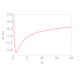
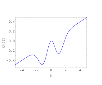
Figure 1: (Color online) The shapes of the anharmonic potentials given by Eqs. (25) and (26) for attractive interactions. Parameter values: $V_{0}=1,\;k=0.1,\;N=4,\;q=1,\;w=5,\;d=5$ and $\gamma=20$.

Figure 1 shows the shapes of the anharmonic potentials $U_{1}(a)$ and $U_{2}(\xi)$ for attractive interactions. As can be seen from this figure, the center-of-mass position of the two-soliton molecule has two local minima. In this case, the two-soliton molecule has a bound state. In Fig. 2, the two-soliton molecule bouncing dynamics over the reflecting potential, modelled by a delta function, are illustrated. The result of numerical solution of the GPE is almost indistinguishable from the prediction of variational approximation.

Figure 2 illustrates the parametric excitation of the two-soliton molecule. Ordinary differential equations (23) and (24) are solved by fourth-order Runge-Kutta method. Numerical solution of the GPE (8) is performed by the split-step fast Fourier transform method.[46]

 

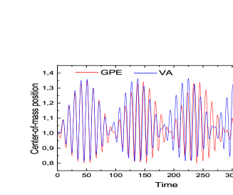
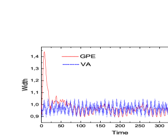
Figure 2: (Color online) Parametric excitation of a two-soliton molecule in a dipolar BEC. Left panel: Numerical solutions of Eqs. (23) and (24) (blue solid line) and the governing GPE (8) (red solid line) for the center-of-mass position of a two-soliton molecule. Right panel: Numerical solutions of the same equations (blue dashed line) and the governing GPE (8) (red solid line) for the width of a two-soliton molecule. Parameters are the same as in Fig. 1.

If the coefficient of nonlocal nonlinearity $\gamma(t)=2d^{2}\rho(t)$ of a system vary periodically with time $\rho(t)=1+\varepsilon\sin(\omega_{0}t+\varphi_{0})$, then an equilibrium position can be unstable, even if it stable for each fixed value of the parameter. This instability is what makes it possible for the parametric excitation of the two-siliton molecule to appear. The phase $\varphi_{0}$ of the parametric oscillations undergoes a jump of $-\pi$ as $\omega_{0}$ passes through the resonance frequency $\omega_{2}$ (see Eq. (30)). When $\omega_{0}$ is near $\omega_{2}$, beats are observed (Fig. 2), i. e., the amplitude of the system alternately waxes when the relation of the phases of the system and the strength of dipolar interactions are such that the strength of dipolar interactions rocks the system, communicating energy to it and wanes when the relation between the phases changes in such a way that the strength of dipolar interactions brakes the system. The closer the frequencies $\omega_{0}$ and $\omega_{2}$, the more slowly the phase relation changes and the large the period of the beats. As $\omega_{0}\rightarrow\omega_{2}$, the period of the beats approaches infinity. Since the resonant frequencies are different for the center-of-mass position $(\omega_{2})$ and width $(\omega_{1}$, see Eq. (29)$)$ of the two-soliton molecule, periodic modulation of the parameter $\gamma(t)$ with the frequency $\omega_{2}$ does not induce resonant oscillations of the width. The jump in width (see the right panel in Fig. 2) can be explained by asymmetric deformation of the two-soliton molecule at the impact with the reflecting potential.

4 Small Amplitude Dynamics

At the present time, problems of nonlinear oscillations have attracted much attention in various spheres of physics. In what follows, we shall consider the dynamics of small nonlinear oscillations of a system about a position of stable equilibrium. Near a position of stable equilibrium, a system executes nonlinear oscillations. It is perfectly natural that the oscillating systems most accessible for investigations are those with small nonlinearity because the methods of the theory of perturbations may be applied to them in some form or the other. Although such an approximation is entirely legitimate when the amplitude of the oscillations is sufficiently small, in higher approximations (called anharmonic oscillations), some minor but qualitatively different properties of the motion appear.[47, 48] Let us examine in detail the case of two 1D systems of eigenfrequencies $\omega_{1}$ and $\omega_{2}$ coupled by an interaction term.

Expanding the coupled system of equations (23) and (24) of two variables into a Taylor’s series in the neighborhood of a point $(a_{0},\,\xi_{0})$, and putting for brevity $x_{1}=a-a_{0}$ and $x_{2}=\xi-\xi_{0}$, we have the following equations of motion:

$$\ddot{x}_{1}+\omega_{1}^{2}x_{1}=\alpha x_{2}^{2},$$ (27)

$$\ddot{x}_{2}+\omega_{2}^{2}x_{2}=\beta x_{1}x_{2}.$$ (28)

Here, the notation is as follows:

$$\omega_{1} = \bigg{\{}\frac{3}{a_{0}^{4}}+\frac{16V_{0}\xi_{0}^{2}}{\sqrt{\pi}a_{0}^{5}}\Big{[}1-\frac{3}{2}(\xi_{0}/a_{0})^{2}+\frac{1}{3}(\xi_{0}/a_{0})^{4}\Big{]}e^{-(\xi_{0}/a_{0})^{2}}+\frac{qN}{2\sqrt{2\pi}a_{0}^{3}}$$ (29)

$$- \frac{\gamma\,N(2a_{0}^{6}-5a_{0}^{4}w^{2}+24a_{0}^{2}w^{4}-4w^{6})}{4\sqrt{2\pi}(a_{0}^{2}+w^{2})^{9/2}}\bigg{\}}^{1/2},$$

$$\omega_{2}=2\big{(}V_{0}/(\sqrt{\pi}a_{0}^{3})\big{)}^{1/2}\Big{[}2(\xi_{0}/a_{0})^{4}-5(\xi_{0}/a_{0})^{2}+1\Big{]}^{1/2}e^{-\frac{1}{2}(\xi_{0}/a_{0})^{2}}.$$ (30)

The frequencies of small amplitude oscillations remain constant during the movement of the system. The system under consideration is weakly coupled. The connection between the frequencies characterizing the state of the system is determined by the approximation $\omega_{1}\approx 2\omega_{2}$. According to the expansion of the coupled system of equations (23) and (24), the coupling coefficients $\alpha$ and $\beta$ are related by the approximation $\beta\approx 2\alpha$. Therefore, using this integrable case, we can obtain meaningful information about the motion of the system by considering the integrable problem in a first approximation.

Stable equilibrium corresponds to a position of the system in which its potential energy is a minimum. We shall measure the potential energy from its minimum value. The solution of Eqs. (27) and (28) may be sought in the form

$$x_{1}(t)=A_{1}(t)e^{i\omega_{1}t}+A_{1}^{\ast}(t)e^{-i\omega_{1}t},$$ (31)

$$x_{2}(t)=A_{2}(t)e^{i\omega_{2}t}+A_{2}^{\ast}(t)e^{-i\omega_{2}t},$$ (32)

where $A_{1}(t)$ and $A_{2}(t)$ are amplitudes of time which vary slowly in comparison with the exponential factors, assuming that $|\ddot{A}_{1}|<<\omega_{1}|\dot{A}_{1}|<<\omega_{1}^{2}|A_{1}|,\;|\ddot{A}_{2}|<<\omega_{2}|\dot{A}_{2}|<<\omega_{2}^{2}|A_{2}|$. This form of solution is, of course, not exact.

Retaining only the terms with $e^{i\omega_{1}t}$ (corresponding $e^{i\omega_{2}t}$) and omitting the $|\ddot{A}_{1}|,\;|\ddot{A}_{2}|$, we have

$$4\omega_{2}\dot{A}_{1}-i\alpha A_{2}^{2}=0,$$ (33)

$$\omega_{2}\dot{A}_{2}-i\alpha A_{1}A_{2}^{\ast}=0.$$ (34)

One sees easily from the coupled system of equations for the amplitudes (33) and (34) that

$$|A_{2}|^{2}+4|A_{1}|^{2}=C_{1}=\mathrm{const},$$ (35)

$$A_{1}A_{2}^{\ast 2}+A_{1}^{\ast}A_{2}^{2}=D_{1}=\mathrm{const}.$$ (36)

The result obtained signify that the quantity (35) is the law of conservation of energy. Now, using Eqs. (33) and (34), one obtains

$$\omega_{2}\frac{d}{dt}|A_{2}|^{2}=i\alpha(A_{1}A_{2}^{\ast 2}-A_{1}^{\ast}A_{2}^{2}).$$ (37)

Squaring Eq. (37) and taking into account Eqs. (35) and (36), we get

$$\Big{(}\frac{d}{dt}|A_{2}|^{2}\Big{)}^{2} = -\frac{\alpha^{2}}{\omega_{2}^{2}}\big{[}(A_{1}A_{2}^{\ast 2}+A_{1}^{\ast}A_{2}^{2})^{2}-4|A_{1}|^{2}|A_{2}|^{4}\big{]}$$ (38)

$$= \frac{\alpha^{2}}{\omega_{2}^{2}}\big{[}(C_{1}-|A_{2}|^{2})|A_{2}|^{4}-D_{1}^{2}\big{]}.$$

Equation (38) is similar to the law of conservation of energy. This equation is similar to equation of motion for a unit mass particle in the anharmonic potential

$$U(|A_{2}|^{2})=(|A_{2}|^{2}-C_{1})|A_{2}|^{4}.$$ (39)

Here, the parameter $|A_{2}|^{2}$ appears as a coordinate.

Figure 3 illustrates the shape of the anharmonic potential $U(|A_{2}|^{2})$. In this figure, a horizontal line corresponds to a given value of the total energy $-D_{1}^{2}$. In Fig. 3, the movement can only occur in the cavity. The points at which the potential energy equals the total energy, i. e. $U(|A_{2}|^{2})=-D_{1}^{2}$ give the limits of the motion.

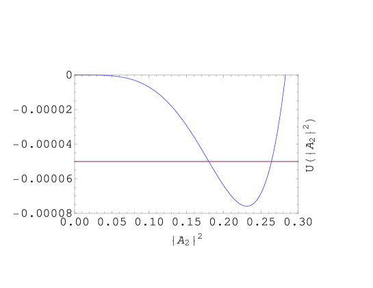
Figure 3: (Color online) The shape of the anharmonic potential $U(|A_{2}|^{2})$ for a given value of the total energy.

A finite motion in one dimension is oscillatory, the particle moving repeatedly back and forth between two points. According to the reversibility property, the time during which the particle passes from $|A_{2,1}|^{2}$ to $|A_{2,2}|^{2}$ and back is twice the time from $|A_{2,1}|^{2}$ to $|A_{2,2}|^{2}$. Thus, the amplitude $|A_{2}|$ oscillates, i.e. beats occur. The dependence of the amplitudes $|A_{1}|$ and $|A_{2}|$ on time can be expressed in terms of elliptic functions.

Note that in contrast to oscillations of linearly coupled oscillators in this case, not only the beat depth but also the period depend on initial amplitudes and phases.

This problem relates to the relationship of longitudinal and transverse oscillations of a $\mathrm{CO_{2}}$ molecule (so-called Fermi resonance).[49] The problem under consideration also occurs in nonlinear optics when the frequency of light doubles and divides.[50]

5 Action-Angle Variables

The Hamiltonian formulation of dynamical equations of physical systems of different nature had a deep impact on the study of dynamical systems. In this section, we shortly recall the “action-angle” variables for the integrable Hamiltonian system. Let us consider the canonical formalism of Hamiltonian system near stationary points. The Hamiltonian of the coupled system of equations (27) and (28) is

$$H=\frac{\dot{x}_{1}^{2}}{2}+\frac{\dot{x}_{2}^{2}}{2}+2\omega_{2}^{2}x_{1}^{2}+\frac{\omega_{2}^{2}x_{2}^{2}}{2}-\alpha x_{1}x_{2}^{2}.$$ (40)

Introducing the canonical variables $x_{i}$ and $p_{i}\equiv\dot{x}_{i}\,(i=1,2)$, Eq. (40) is reduced to the Hamiltonian

$$H=\frac{1}{2}\big{(}p_{1}^{2}+p_{2}^{2}+4\omega_{2}^{2}x_{1}^{2}+\omega_{2}^{2}x_{2}^{2}\big{)}-\alpha x_{1}x_{2}^{2}.$$ (41)

In action-angle variables $(I_{i},\theta_{i})$ introduced as[51]

$$x_{i}=\sqrt{2I_{i}/\omega_{i}}\sin\theta_{i},\quad p_{i}=\sqrt{2I_{i}\omega_{i}}\cos\theta_{i},$$ (42)

the Hamiltonian can be rewritten as

$$H=2I_{1}\omega_{2}+I_{2}\omega_{2}-\frac{2\alpha I_{2}}{\omega_{2}}\sqrt{\frac{I_{1}}{\omega_{2}}}\,\sin\theta_{1}\sin^{2}\theta_{2}.$$ (43)

Hamilton’s equations $\dot{\theta}_{i}=\partial H/\partial I_{i},\;\dot{I}_{i}=-\partial H/\partial\theta_{i}$ for action-angle variables $(I_{i},\theta_{i})$ yield the following two pairs of coupled equations:

$$\dot{I}_{1} = \frac{2\alpha I_{2}}{\omega_{2}}\sqrt{\frac{I_{1}}{\omega_{2}}}\,\sin^{2}\theta_{2}\cos\theta_{1},$$ (44)

$$\dot{\theta}_{1} = 2\omega_{2}-\frac{\alpha I_{2}}{\omega_{2}\sqrt{\omega_{2}I_{1}}}\,\sin^{2}\theta_{2}\sin\theta_{1}$$ (45)

and

$$\dot{I}_{2} = \frac{2\alpha I_{2}}{\omega_{2}}\sqrt{\frac{I_{1}}{\omega_{2}}}\,\sin\theta_{1}\sin 2\theta_{2},$$ (46)

$$\dot{\theta}_{2} = \omega_{2}-\frac{2\alpha}{\omega_{2}}\sqrt{\frac{I_{1}}{\omega_{2}}}\,\sin\theta_{1}\sin^{2}\theta_{2}.$$ (47)

Let us now consider the stationary points. When the action is $\dot{I}_{1}=0$, then the stationary value of angle is $\theta_{01}=\pi/2$. Thus, the stationary value of action is $I_{01}=\big{(}\alpha I_{2}\sin^{2}\theta_{2}/\big{(}2\omega_{2}^{5/2}\big{)}\big{)}^{2}$ at fixed values $I_{2},\theta_{2}$. In the second pair of coupled equations (46) and (47), when $\dot{I}_{2}=0$, we obtain $\theta_{02}=0$ and $\theta_{02}=\arcsin\big{[}\big{(}\omega_{2}^{2}\sqrt{\omega_{2}/I_{1}}/(2\alpha)\big{)}^{1/2}\big{]}$ at fixed value $I_{1}$. Let us find the numerical solutions of the first pair of coupled equations (44) and (45) for the action $I_{1}(t)$ and angle $\theta_{1}(t)$ variables of Hamiltonian system. In Fig. 4, we represent the evolution of the angle variable and oscillations of the action.

 

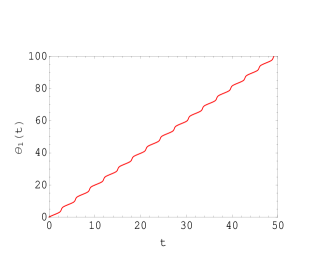
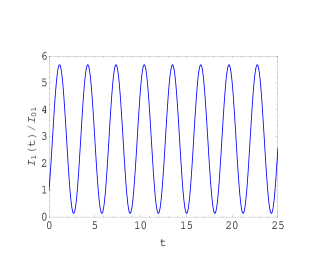
Figure 4: (Color online) Left panel: Evolution of the angle variable $\theta_{1}(t)$ (red solid line). Right panel: Oscillations of the action variable $I_{1}(t)$ (blue solid line) normalized to $I_{01}$.

The formulation of Hamiltonian equations in action-angle variables is most convenient to study Hamiltonian systems in the presence of perturbations and to construct symplectic maps.[52] The difficulty of quantizing non-integrable systems was expressed in terms of the invariant tori of action-angle variables. The use of action-angle variables was central to the solution of the Toda lattice,[53] and to the definition of Lax pairs.[54]

6 Stationary State of a Two-Soliton Molecule

Below, we consider the stationary width of a two-soliton molecule. Equation (23), which allows us to find the stationary solution of the one-dimensionless nonlocal GPE (8) and describes its dynamics near the fixed point, is the main result of this section. At large deviations from the stationary state, the waveform (10) can be deviated from the Gauss-Hermite shape, and the predictions of the variational approximation become less accurate.

The stationary width of a two-soliton molecule $a_{0}$ is calculated from the following condition:

$$\frac{a_{0}^{4}(a_{0}^{4}+4w^{4})}{(a_{0}^{2}+w^{2})^{7/2}}-\frac{q}{\gamma}\,a_{0}-\frac{16\sqrt{2}V_{0}\xi_{0}^{2}}{\gamma\,Na_{0}}\Big{(}1-\frac{2\xi_{0}^{2}}{3a_{0}^{2}}\Big{)}e^{-(\xi_{0}/a_{0})^{2}}-\frac{4\sqrt{2\pi}}{\gamma\,N}=0.$$ (48)

Figure 5 illustrates the frequency of small amplitude oscillations of the two-soliton molecule as a function of the strength of contact interactions, according to Eq. (29). The same figure shows the stationary width of the two-soliton molecule for a given strength of contact interactions, obtained from Eq. (48).

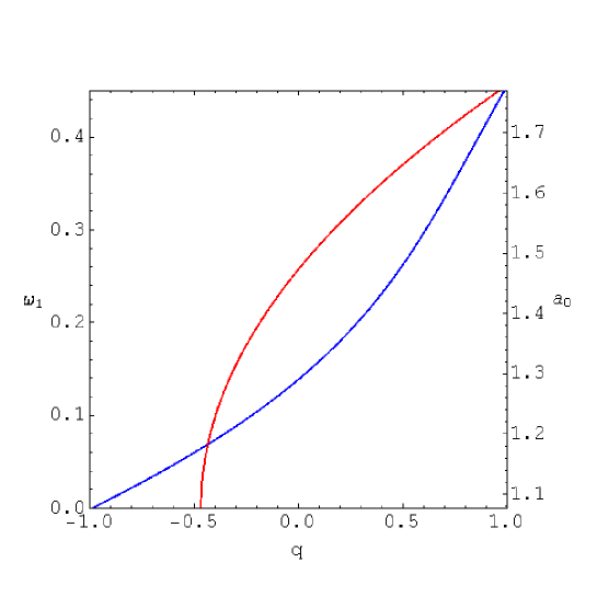
Figure 5: (Color online) The frequency of low energy shape oscillations $(\omega_{1})$ of a two-soliton molecule in a dipolar BEC as a function of the strength of contact interactions $q$, according to Eq. (29) (red solid line), and the stationary width of a two-soliton molecule ($a_{0})$ obtained from Eq. (48) (blue line). Parameter values: $V_{0}=1,\,N=4,\,w=5$ and $\gamma=20$.

The case of repulsive contact interactions $(q<0)$ give rise to decreasing of the frequency of oscillations compared to the case of pure dipolar interactions $(q=0)$, while the contribution of attractive interactions $(q>0)$ is opposite, leading to increasing of the oscillations frequency.

Low energy collective oscillations of ultracold atoms can provide essential information about the interatomic forces in BEC.[55] As a result, the expression (29) for the frequency of the small amplitude oscillations of the two-soliton molecule can be useful in experiments with ultracold polar molecules.

In nonlinear wave equations, the stability of localized solutions can be examined by means of the Vakhitov-Kolokolov criterion.[56] Using the usual procedure,[57] we look for the stationary solution of the one-dimensionless nonlocal GPE (8) in the form $\psi(x,t)=e^{-i\mu t}\zeta(x)$, with $\mu$ denoting the chemical potential.

The time-independent one-dimensionless nonlocal GPE (8) takes the form

$$\big{(}\mu-kx-V(x)\big{)}\zeta+\frac{1}{2}\,\zeta_{xx}-q\,\zeta^{3}+\gamma\zeta\int\limits_{-\infty}^{\infty}R(|x-z^{\prime}|)\zeta^{2}(z^{\prime})dz^{\prime}=0.$$ (49)

The corresponding Lagrangian density is

$${\cal L}=\frac{1}{4}\Big{[}\zeta_{x}^{2}-2\big{(}\mu-kx-V(x)\big{)}\zeta^{2}+q\,\zeta^{4}-\gamma\zeta^{2}\int\limits_{-\infty}^{\infty}R(|x-z^{\prime}|)\zeta^{2}(z^{\prime})dz^{\prime}\Big{]}.$$ (50)

We seek a solution in the form:

$$\zeta(x)=A(x-\xi)\exp\Big{[}{-\frac{(x-\xi)^{2}}{2a^{2}}}\Big{]}.$$ (51)

Substituting the trial function (51) and using the response function (9) into the Lagrangian density (50) and subsequently integrating over the space variable, we obtain the following averaged Lagrangian

$$L = \frac{3\sqrt{\pi}A^{2}a}{16}-\frac{\sqrt{\pi}\mu A^{2}a^{3}}{4}+\frac{\sqrt{\pi}kA^{2}a^{3}\xi}{4}+\frac{V_{0}A^{2}\xi^{2}}{2}\,e^{-(\xi/a)^{2}}$$ (52)

$$+ \frac{3\sqrt{\pi/2}\,qA^{4}a^{5}}{64}-\frac{\sqrt{\pi/2}\,\gamma A^{4}a^{6}}{64}\bigg{[}\frac{4w^{2}(a^{2}+w^{2})+3a^{4}}{(a^{2}+w^{2})^{5/2}}\bigg{]}.$$

Performing further the standard variational approximation procedure,[39, 40] we obtain the following functions of the variable $a$ for the chemical potential and norm:

$$\mu(a) = \frac{1}{2a^{2}}+k\,\xi_{0}+\frac{V_{0}\xi_{0}^{2}}{\sqrt{\pi}a^{3}}\Big{(}1+\frac{2\xi_{0}^{2}}{3a^{2}}\Big{)}e^{-(\xi_{0}/a)^{2}}+\frac{11q\,N}{16\sqrt{2\pi}a}$$ (53)

$$- \frac{\gamma\,N}{16\sqrt{2\pi}}\bigg{[}\frac{11a^{6}+28a^{2}w^{2}(a^{2}+w^{2})+16w^{6}}{(a^{2}+w^{2})^{7/2}}\bigg{]},$$

$$N(a)=\frac{8\big{[}3\sqrt{\pi}a^{3}+4V_{0}\xi_{0}^{2}(3a^{2}-2\xi_{0}^{2})e^{-(\xi_{0}/a)^{2}}(a^{2}+w^{2})^{7/2}\big{]}}{3\sqrt{2}a^{4}\big{[}\gamma\,a^{3}(a^{4}+4w^{4})-q(a^{2}+w^{2})^{7/2}\big{]}}.$$ (54)

We have established a connection between the chemical potential and the norm.[34] According to Vakhitov-Kolokolov criterion[56] $\frac{d\mu}{dN}<0$, we obtained the stability of the two-soliton molecule. It should be noted that for the repulsive contact interactions $(q<0)$, pure dipolar interactions $(q=0)$ and the effect of attractive interactions $(q>0)$, the two-soliton molecule remains stable for different values of the nonlocal coefficient $\gamma\,(\gamma>0)$. The stronger attraction between solitons leads to more stability of the molecule.[11]

7 Conclusion

The model of a “quantum bouncer” has been extended to a dipolar BECs. We have studied the effects of atomic dipole-dipole interactions and gravity on the dynamics of BECs by means of variational approximation and numerical simulations. In numerical experiments, we observed the parametric excitation by a two-soliton molecule when the vertical position of the atomic mirror is periodically varied in time. We have provided thorough comparison between the results of variational approximation and numerical simulations of the GPE. We have studied Hamilton’s dynamic system for a dipolar condensates in terms of “action-angle” variables. In this paper, the stationary state of a two-soliton molecule in a dipolar BECs has been studied.

References

References

- [1] M. H. Anderson, J. R. Ensher, M. R. Matthews, C. E. Wieman, and E. A. Cornell, Science 269 (1995) 198.
- [2] K. B. Davis, M.-O. Mewes, M. R. Andrews, N. J. van Druten, D. S. Durfee, D. M. Kurn, and W. Ketterle, Phys. Rev. Lett. 75 (1995) 3969.
- [3] C. C. Bradley, C. A. Sackett, J. J. Tollett, and R. G. Hulet, Phys. Rev. Lett. 75 (1995) 1687.
- [4] A. Einstein, Sitzungsber. Preuss. Akad. Wiss. 23 (1925) 18.
- [5] S. N. Bose, Z. Phys. 26 (1924) 178.
- [6] C. E. Hecht, Physica 25 (1959) 1159.
- [7] W. C. Stwalley, L. H. Nosanow, Phys. Rev. Lett. 36 (1976) 910.
- [8] D. G. Fried, T. C. Killian, L. Willmann, D. Landhuis, S. C. Moss, D. Kleppner, T. J. Greytak, Phys. Rev. Lett. 81 (1998) 3811.
- [9] J. Klaers, J. Schmitt, F. Vewinger, M. Weitz, Nature 468 (2010) 545.
- [10] J. Doyle, B. Friedrich, R. V. Krems, and F. Masnou-Seeuws, Eur. Phys. J. D 31 (2004) 149.
- [11] T. Lahaye, C. Menotti, L. Santos, M. Lewenstein and T. Pfau, Rep. Prog. Phys. 72 (2009) 126401.
- [12] J. Deiglmayr, A. Grochola, M. Repp, K. Mrtlbauer, C. Glck, J. Lange, O. Dulieu, R. Wester, and M. Weidemller, Phys. Rev. Let. 101 (2008) 133004.
- [13] M. Stratmann, T. Pagel, and F. Mitschke, Phys. Rev. Let. 95 (2005) 143902.
- [14] M. Guo, X. Ye, J. He, G. Qumner, and D. Wang, Phys. Rev. A 97 (2018) 020501(R).
- [15] A. Griesmaier, J. Werner, S. Hensler, J. Stuhler, and T. Pfau, Phys. Rev. Lett. 94 (2005) 160401.
- [16] Q. Beaufils, R. Chicireanu, T. Zanon, B. Laburthe-Tolra, E. Marchal, L. Vernac, J.-C. Keller, and O. Gorceix, Phys. Rev. A 77 (2008) 061601(R).
- [17] M. Lu, N. Q. Burdick, S. H. Youn and B. L. Lev, Phys. Rev. Lett. 107 (2011) 190401.
- [18] K. Aikawa, A. Frisch, M. Mark, S. Baier, A. Rietzler, R. Grimm and F. Ferlaino, Phys. Rev. Lett. 108 (2012) 210401.
- [19] P. O. Schmidt, S. Hensler, J. Werner, A. Griesmaier, A. Gorlitz, T. Pfau, and A. Simoni, Phys. Rev. Lett. 91 (2003) 193201.
- [20] J. Stuhler, A. Griesmaier, T. Koch, M. Fattori, T. Pfau, S. Giovanazzi, P. Pedri, and L. Santos, Phys. Rev. Lett. 95 (2005) 150406.
- [21] A. Benseghir, W. A. T. Wan Abdullah, B. B. Baizakov, and F. Kh. Abdullaev, Phys. Rev. A 90 (2014) 023607.
- [22] N. V. Vysotina, N. N. Rosanov, JETP 123 (2016) 51.
- [23] J. Akram, B. Girodias, A. Pelster, J. Phys. B, At. Mol. Opt. Phys. 49 (2016) 075302.
- [24] Golam Ali Sekh, Phys. Lett. A 381 (2017) 852.
- [25] R. L. Gibbs, Am. J. Phys. 43 (1975) 25.
- [26] P. W. Langhoff, Am. J. Phys. 39 (1974) 954; R. D. Desko and D. J. Bord, ibid. 51 (1983) 82; D. A. Goodings and T. Szeredi, ibid. 59 (1991) 924; J. Gea-Banacloche, Opt. Commun. 179 (2000) 117; S. Whineray, Am. J. Phys. 60 (1992) 948; M. A. Doncheski and R. W. Robinett, ibid. 69 (2001) 1084.
- [27] J. Gea-Banacloche, Am. J. Phys. 67 (1999) 776.
- [28] R. W. Robinett, Eur. J. Phys. 31 (2010) 1; M. Belloni and R. W. Robinett, Phys. Rep. 540 (2014) 25.
- [29] A. M. Dikand, I. N. Ngek and J. Ebobenow, Mod. Phys. Lett. B 24 (2010) 2911.
- [30] M. Morinaga, M. Yasuda, T. Kishimoto, F. Shimizu, J. Fujita and S. Matsui, Phys. Rev. Lett. 77 (1996) 802; F. Shimizu, Mater. Sci. Eng. B 48 (1997) 7.
- [31] M. O. Mewes et al., Phys. Rev. Lett. 78 (1997) 582; I. Bloch et al., Phys. Rev. Lett. 82 (1999) 3008.
- [32] Y. Le Coq et al., Phys. Rev. Lett. 87 (2001) 170403; N. P. Robins, A. K. Morrison, J. J. Hope and J. D. Close, Phys. Rev. A 72 (2005) 031606.
- [33] L. P. Pitaevskii and S. Stringari, Bose-Einstein Condensation (Clarendon Press, Oxford, 2003).
- [34] C. J. Pethick and H. Smith, Bose-Einstein Condensation in Dilute Gases (Cambridge University Press, Cambridge, 2002).
- [35] S. Sinha, L. Santos, Phys. Rev. Lett. 99 (2007) 140406.
- [36] W. Ketterle, Rev. Mod. Phys. 74 (2002) 1131.
- [37] E. A. Cornell, C. E. Wieman, Rev. Mod. Phys. 74 (2002) 875.
- [38] V. V. Nesvizhevsky, Phys. Usp. 47 (2004) 515; V. V. Nesvizhevsky, Phys. Usp. 53 (2010) 645.
- [39] D. Anderson, Phys. Rev. A 27 (1983) 1393.
- [40] B. A. Malomed, Progr. Opt. 43 (2002) 69.
- [41] G. Assanto, Nematicons: Spatial Optical Solitons in Nematic Liquid Crystals (John Wiley and Sons, Inc., Hoboken, New Jersey, 2013).
- [42] J. Cuevas, B. A. Malomed, P. G. Kevrekidis, and D. J. Frantzeskakis, Phys. Rev. A 79 (2009) 053608.
- [43] I. N. Ngek, A. M. Dikand, and A. B. Moubissi, J. Phys. Soc. Jpn. 85 (2016) 124002.
- [44] T. I. Lakoba and D. J. Kaup, Phys. Rev. E 58 (1998) 6728.
- [45] F. Kh. Abdullaev, V. A. Brazhnyi, J. Phys. B: At. Mol. Opt. Phys. 45 (2012) 085301.
- [46] W. H. Press, S. A. Teukolsky, W. T. Vetterling and B. P. Flannery, Numerical Recipes. The Art of Scientific Computing (Cambridge University Press, Cambridge, 1996).
- [47] N. N. Bogoliubov and Y. A. Mitropolsky, Asymptotic Methods in the Theory of Non-Linear Oscillations (Hindustan Publishing Corporation, Delhi, 1961).
- [48] J. J. Stoker, Nonlinear Vibrations in Mechanical and Electrical Systems (Interscince Publishers, New York, 1950).
- [49] E. Fermi, Memorie. Accad. d’Italia 3 (1932) 239; E. Fermi, Z. Phys. 71 (1931) 250; E. Fermi, F. Rasetti, Z. Phys. 71 (1931) 689.
- [50] N. Bloembergen, Nonlinear Optics (W. A. Benjamin, Inc. New York-Amsterdam, 1965).
- [51] L.D. Landau, E. M. Lifshitz, Mechanics (Butterworth-Heinemann, London, 2000).
- [52] G. M. Zaslavsky, B. V. Chirikov, Sov. Phys. Usp. 14 (1972) 549.
- [53] M. Toda, J. Phys. Soc. Jpn. 22 (1967) 431.
- [54] P. D. Lax, Comm. Pure Appl. Math. 21 (1968) 467.
- [55] D. S. Jin, J. R. Ensher, M. R. Matthews, C. E. Wieman and E. A. Cornell, Phys. Rev. Lett. 77 (1996) 420.
- [56] N. G. Vakhitov, A. A. Kolokolov, Radiophys. Quantum Electron. 16 (1973) 783.
- [57] F. Kh. Abdullaev, Nonlinear Matter Waves in Cold Quantum Gases (International Islamic University Malaysia, Kuala Lumpur, Malaysia, 2005).