Resummed predictions for jet-resolution scales in multijet production in $e^{+}e^{-}$ annihilation

Abstract

We present for the first time resummed predictions at $\mathrm{NLO+NLL}^{\prime}$ accuracy for the Durham jet-resolution scales $y_{n,n+1}$ in multijet production in $e^{+}e^{-}$ collisions. Results are obtained using an implementation of the well known CAESAR formalism within the SHERPA framework. For the 4-, 5- and 6-jet resolutions we discuss in particular the impact of subleading colour contributions and compare to matrix-element plus parton-shower predictions from SHERPA and VINCIA.

1 Introduction

Jet-production processes provide direct means to investigate the dynamics of the strong interaction. Especially multijet production poses a severe multi-scale problem complicating theoretical analyses. Besides integrated jet rates, differential distributions of jet-resolution scales give insight into the mechanism of jet production for a given jet-clustering algorithm. While for well-separated energetic jets a fixed-order QCD estimation might be adequate, in particular for small jet-resolutions this is bound to fail and all-orders resummation techniques need to be employed to provide reliable theoretical predictions. These account for soft and collinear QCD radiation that dominates the emission spectrum.

While jet rates are of phenomenological importance both at lepton and hadron colliders, we here focus on the resummation of jet-resolution scales in multijet production in $e^{+}e^{-}$ annihilation. In particular, we consider the Durham jet algorithm [1], where the jet-resolution parameter is determined by

$$y_{ij}=\frac{2\min(E^{2}_{i},E^{2}_{j})}{Q^{2}}(1-\cos\theta_{ij})\,.$$ (1)

Here, $E_{i,j}$ denote the energies of (pseudo) particles $i$ and $j$, $\theta_{ij}$ the angle between them, and $Q^{2}$ the squared centre-of-mass energy. This measure is used to successively cluster particles into jet objects. In what follows, we are interested in the resolution scales where an $(n+1)$-jet final state is clustered in an $n$-jet final state, i.e., where the emission of an additional jet off the $n$-jet configuration gets resolved. More precisely, we consider the differential $3\to 4$, $4\to 5$ and $5\to 6$ jet resolutions at next-to-leading logarithmic accuracy, i.e., resumming leading logarithms (LL) of type $\alpha_{\text{s}}^{k}L^{k+1}$ and next-to-leading logarithms (NLL) $\alpha_{\text{s}}^{k}L^{k}$ with $L\equiv-\ln(y_{n,n+1})$ appearing in the exponent of the observable’s cummulant distribution. For many observables in $e^{+}e^{-}$ annihilation, there exist results at NLL, NNLL or even N³LL order matched to exact NLO or NNLO QCD matrix elements, see for instance [2, 3, 4, 5, 6, 7, 8, 9, 10, 11]. However, these are limited to two- or three-jet final states. Here, we are in particular exploring high-multiplicity processes, i.e., jet emission from $4$- and $5$-jet matrix elements that feature Born processes with non-trivial colour configurations. For the three-jet resolution $y_{23}$, NLL resummed predictions were calculated in [12]; NNLL+NNLO results were presented in [13]. This observable in particular has been used in extractions of the strong coupling constant $\alpha_{\text{s}}$ from LEP data, see for instance [14, 15, 16]. Recently, in Ref. [17], the extraction of $\alpha_{\text{s}}$ from a simultaneous fit of the two- and three-jet rates has been presented. However, in this study the three-jet rate has been considered at fixed-order NNLO QCD without resummation of logarithmic enhanced terms. Up to now, for Durham three- and higher jet rates only the next-to-double-leading logarithms of order $\alpha_{\text{s}}^{k}L^{2k-1}$ have been calculated [1]. In [18] this has been extended to the generalised class of $k_{T}$-type algorithms defined in [19]. Besides for the extractions of $\alpha_{\text{s}}$, integrated and differential jet rates prove to be very useful for theoretical validation of parton-shower algorithms [18, 20]. Corresponding experimental measurement data from the LEP experiments, see for example [21, 22], form an integral ingredient to event generator tuning efforts, as they provide handles to constrain the parameters of phenomenological hadronisation models, see Ref. [23] for a review.

To achieve NLL resummation for jet resolutions, we rely on an independent implementation of the CAESAR formalism [24, 25] in the SHERPA [26, 27] event-generator framework, presented in [28]. A brief introduction to the CAESAR approach and details on the implementation of automated NLL resummation in the SHERPA framework are discussed in Sec. 2. This includes a brief presentation of the approach used to match our resummed predictions to exact QCD matrix elements. In Sec. 3, we give specific algorithmic details on the actual resummation of jet-resolution scales and discuss the validation of the soft function and the multiple-emission contribution in particular.

In Sec. 4, we present our resummed predictions for jet production off $3-,4-$ and $5-$jet final states in $e^{+}e^{-}$ annihilation. To this end we evaluate the jet resolutions $y_{34}$, $y_{45}$ and $y_{56}$ at NLL accuracy, matched to exact $4-,5-$ and $6-$jet NLO QCD matrix elements, respectively. We give an account of subleading-colour contributions, by comparing our full-colour results to the strict and an improved large-$N_{\text{C}}$ approximation, the latter corresponding to what is typically used in QCD parton showers. Finally, we compare the $\mathrm{NLO}+\mathrm{NLL}^{\prime}$ results to matrix-element-plus-parton-shower simulations from SHERPA and VINCIA, where we also address the impact of hadronisation corrections on the observables. We present our conclusions and an outlook in Sec. 5.

2 Semi-automated resummation within the SHERPA framework

In Ref. [28], an implementation of the CAESAR formalism in the form of a plugin to the SHERPA event-generator framework has been presented, which we employ for resummation of Durham jet-resolutions. A particular focus has there been put on validating the colour decomposition of hard-scattering matrix elements and the colour-insertion operators for multi-parton processes. The resummation plugin has since been used for NLL resummation of the thrust event-shape variable in $e^{+}e^{-}$, $ep$ and $pp$ collisions [28], with results matched to tree-level real-emission matrix elements using a point-wise local subtraction technique. Recently, the implementation has also been used to resum the soft-drop thrust shape in $e^{+}e^{-}$ annihilation [29].

In this section, we briefly review the CAESAR formalism and comment on specific implementation aspects. Details on the application to resummation of jet-resolution scales will then be provided in Sec. 3.

2.1 The CAESAR formalism in a nutshell

The CAESAR formalism has originally been presented for final-state resummation in [24]; its extension to hadronic initial-states has been worked out in [30, 31]. For an extensive review we refer to [25]. The method provides all necessary ingredients to perform NLL resummed calculations of recursively infrared and collinear safe global observables in a largely automated manner. The method is based on the observation that for the wide class of global event-shape observables, the resummed cumulative distribution for the observable value $V\leq v$ can, to NLL accuracy, be expressed in the simple form

$$\begin{split}\Sigma_{\mathrm{res}}(v)&=\sum_{\delta}\Sigma^{\delta}(v)\,,\,\,\text{where}\\ \Sigma_{\mathrm{res}}^{\delta}(v)&=\int d\mathcal{B_{\delta}}\frac{\mathop{d\sigma_{\delta}}}{\mathop{d\mathcal{B_{\delta}}}}\exp\left[-\sum_{l\in\delta}R_{l}^{\mathcal{B_{\delta}}}(L)\right]\mathcal{S}^{\mathcal{B_{\delta}}}(L)\mathcal{F}^{\mathcal{B_{\delta}}}(L)\mathcal{H}^{\delta}(\mathcal{B_{\delta}})~{},\hskip 28.45274ptL\equiv\ln 1/v\end{split}$$ (2)

where the phase-space integral extends over the Born configurations $\mathcal{B}$ for each partonic channel $\delta$. Dependence of the various contributions on those will implicitly be assumed in the following, although labels will be dropped. The jet-function $\mathcal{H}$ implements kinematic cuts on the Born events and ensures that only sufficiently hard configurations yield non-zero contributions. In the exponent, the collinear radiators for all hard legs $l$ are summed. The function $\mathcal{F}$ accounts for the effect of multiple emissions, whereas the soft function $\mathcal{S}$ captures colour correlations. Its logarithmic dependence is defined via

$$\mathcal{S}(L)=S\left(T(L)\right)\,,\quad\text{with}\quad T(L)=-\frac{1-\frac{2}{a}\lambda}{\pi\beta_{0}}\,,$$ (3)

where the parameter $\lambda$ is given by $\lambda=\alpha_{\text{s}}(\mu_{R}^{2})\beta_{0}L$.

In [25] the functions $R_{l}$ have been evaluated for the general class of observables $V$, where the impact of one additional, arbitrarily soft, emission with momentum $k$ off leg $l$ can be parameterised as

$$V(k)=d_{l}(\mu_{Q})g_{l}(\phi_{l})\left(\frac{k_{\mathrm{T},l}}{\mu_{Q}}\right)^{a}e^{-b_{l}\eta_{l}}\,,$$ (4)

i.e., in terms of the transverse momentum $k_{\mathrm{T},l}$, rapidity $\eta_{l}$, and azimuth $\phi_{l}$ of the emission, measured with respect to leg $l$. Here, $\mu_{Q}$ denotes the, in principle arbitrary, resummation ”starting”-scale, to be distinguished from the centre-of-mass energy $Q$. Independence of the observable from the unphysical scale $\mu_{Q}$ implies $d_{l}\propto\mu_{Q}^{a}$. Explicit results for the radiators can be found in the appendix of [25].

2.2 Aspects of automated NLL resummation

The CAESAR formalism is ideally suited for the automation of resummation of appropriate observables. With the observable parametrisation in terms of $a$, $b_{l}$, $d_{l}$ and $g_{l}$, the radiator functions are known. The colour decomposition of the Born process in a suitable basis and the corresponding soft-gluon correlators, needed for constructing the soft-function $\mathcal{S}$, are independent of the actual observable to be resummed and can thus be pre-computed. The required Born-process partial amplitudes can be obtained from an automated matrix-element generator such as COMIX [32] for, in principle, arbitrary processes. However, the colour-space dimensionality quickly grows with the number of external partons [28], making calculations for high-multiplicity processes memory-intense. This motivates the construction of optimal, i.e., minimal-dimensional and orthogonal, bases, see Ref. [33, 34, 35]. An observable-dependent component that needs special attention is the multiple-emission function $\mathcal{F}$, for that one often has to resort to numerical evaluations, which can, however, be pre-computed and tabulated. Here, we briefly introduce $\mathcal{S}$ and $\mathcal{F}$ in general terms, before discussing specific aspects and their validation for the resummation of jet-resolution scales in Sec. 3.

The soft function $S$

The automated generation of the soft-function $S$ as defined in Eq. (3) for arbitrary multiplicity Born processes has been discussed in detail in Ref. [28]. Here, we only want to review some general aspects and briefly discuss the specific colour spaces we face for the case of multijet production in $e^{+}e^{-}$ annihilation.

The functional form of $S$ is given by

$$\begin{split}S(t)=\frac{\expectationvalue{e^{-\frac{t}{2}\Gamma^{\dagger}}e^{\frac{t}{2}\Gamma}}{\mathcal{B}}}{\innerproduct{\mathcal{B}}{\mathcal{B}}}\,,\end{split}$$ (5)

with $\ket{\mathcal{B}}$ the Born-process matrix element and $\Gamma$ the soft anomalous-dimension matrix, cf. Eq. (10). By decomposing the Born matrix element over a colour basis,

$$\ket{\mathcal{B}}=\sum\limits_{\alpha}\mathcal{A}_{\alpha}\ket{b_{\alpha}},$$ (6)

and making a particular choice $\{\ket{b_{\alpha}}\}$ for the colour structures of the Born process, we can define a metric

$$c_{\alpha\beta}=\innerproduct{b_{\alpha}}{b_{\beta}}$$ (7)

and its inverse $c^{\alpha\beta}$. This allows us to write

$$\innerproduct{\mathcal{B}}{\mathcal{B}}=\Tr\left[cH\right]$$ (8)

with the hard matrix $H_{\alpha\beta}=\overline{\mathcal{A}}_{\alpha}\mathcal{A}_{\beta}$ in terms of partial amplitudes $\mathcal{A}_{\gamma}$. In this notation, the soft function may be written as

$$S(t)=\frac{\Tr\left[He^{-\frac{t}{2}\Gamma^{\dagger}}ce^{-\frac{t}{2}\Gamma}\right]}{\Tr\left[cH\right]}\,,$$ (9)

with

$$\Gamma=-2\sum_{i<j}\boldsymbol{T}_{i}\boldsymbol{T}_{j}\ln\frac{Q_{ij}}{Q}+\text{i}\pi\sum_{\begin{subarray}{c}ij=\\ II,FF\end{subarray}}\boldsymbol{T}_{i}\boldsymbol{T}_{j}\,.$$ (10)

Here, the first sum runs over all colour dipoles $ij$, while the second one runs over those consisting only of final-final or inital-initial configurations, corresponding to the exchange of Coulomb gluons [36]. Explicit results for $H$, $c$, and $\Gamma$ are known for up to four hard (coloured) legs; the form of $S$ and the structure of $\Gamma$, however, holds more generally [37].

We obtain the hard matrix $H$ from the matrix-element generator COMIX [32] that is part of SHERPA. All calculations of colour correlators relevant here contain at least one quark-antiquark pair and are performed in the trace basis. An all-orders trace basis is obtained by connecting each quark with an antiquark in all possible ways and subsequently attaching all gluons in all possible ways. Colour correlators are then evaluated by explicitly employing $\text{SU}(N_{\text{C}})$ identities. We note that this slightly differs from the approach in the COLORFULL [38] package, which uses specialised replacements in the trace basis instead.

Table 1: Colour-space and corresponding bases dimensionalities for all relevant Born channels.

	Dimension
Process $e^{+}e^{-}\to$	$q\bar{q}g$	$q\bar{q}q\bar{q}$	$q\bar{q}gg$	$q\bar{q}q\bar{q}g$	$q\bar{q}ggg$
Colour Space	1	2	3	4	10
Trace Basis	1	2	3	4	11
Reduced Trace Basis	1	2	3	4	10

One problem arising in the context of trace bases is that these are generally overcomplete for $n_{q\bar{q}}+n_{g}>N_{\text{C}}$, such that the metric defined in Eq. (7) does not possess a unique inverse. Although this has generally been solved in Ref. [28], within this study we can circumvent it in an even simpler way. The only critical process is $e^{+}e^{-}\to q\bar{q}+3g$ (cf. Tab. LABEL:tab:colour_dimensions), for which the dimensionality of the basis exceeds the dimensionality of the colour space by one. Thus, we are able to define a basis with lower dimension by combining basis vectors corresponding to the same partial amplitude, i.e.,

$$\ket{\tilde{b}_{\alpha}}\mathrel{\mathop{\mathchar 58\relax}}=\ket{b_{1,2,\ldots,m}}+(-1)^{m}\ket{b_{1,m,\ldots,2}}\equiv\Tr[T_{i_{1}}T_{i_{2}}\cdots T_{i_{m}}]+(-1)^{m}\Tr[T_{i_{1}}T_{i_{m}}\cdots T_{i_{2}}]\,.$$ (11)

We refer to this as the “reduced trace basis”. In Sec. 3.2, we report on the validation of the colour correlators for the specific processes under investigation.

The multiple-emission function $\mathcal{F}$

The component $\mathcal{F}$ of Eq. (2) captures the effect of multiple emissions on the cumulative distribution $\Sigma$. Recursive infrared collinear safety of the observable guarantees that one can treat emissions below a cutoff $\epsilon$ as unresolved, such that the cancellation between real and virtual corrections is complete. To eliminate subleading terms, one would usually have to find suitable integral transforms to factorise the contributions of multiple individual emissions. This is for example straightforward for additive observables, $V(k_{1},\dots,k_{m})=\sum_{i=1}^{m}V(k_{i})$, where one can insert a simple integral representation of the corresponding $\Theta$-function. In general, this procedure can however yield rather untractable expressions, or there are no such transformations known as is the case for the jet-resolution scales. In those cases, one can resort to numerical evaluations, rescaling momenta to eliminate contributions that vanish in the strict soft limit. In [25] a general form of the multiple-emission function $\mathcal{F}$ suitable for numerical evaluation was derived. It was in particular used to resum $y_{23}$ to NLL [12] and (with suitable additions) NNLL in [13] accuracy. The general formula for a specific flavour channel $\delta$ reads

$$\begin{split}\mathcal{F}^{\mathcal{B}_{\delta}}(L)=\lim_{\epsilon\rightarrow 0}e^{R^{\prime}\,\ln\epsilon}\sum_{m=0}^{\infty}\frac{R^{\prime m}}{m!}\left(\prod_{i=1}^{m+1}\sum_{l_{i}\in\delta}\frac{R^{\prime}_{l_{i}}}{R^{\prime}}\right.&\left.\int_{\epsilon}^{1}\frac{\mathop{d\zeta_{i}}}{\zeta_{i}}\int_{0}^{1}\frac{\mathop{d\xi_{i}}}{\mathcal{N}_{l_{i}}}\int_{0}^{2\pi}\frac{\mathop{d\phi_{i}}}{2\pi}\right)\delta(\text{ln}\zeta_{1})\\ &\times\text{exp}\left(-R^{\prime}\,\ln\lim_{\bar{v}\rightarrow 0}\frac{V(\mathcal{B}_{\delta};\kappa_{1}(\zeta_{1}\bar{v}),...,\kappa_{m+1}(\zeta_{m+1}\bar{v}))}{\bar{v}}\right),\end{split}$$ (12)

$$\text{with}\hskip 28.45274pt\mathcal{N}_{l_{i}}=\left(1+\frac{a+(1-\xi_{i})b_{l_{i}}}{a(a+b_{l_{i}})}2\lambda\right)\int_{0}^{1}\text{d}\tilde{\xi}_{i}\frac{1}{1+\frac{a+(1-\tilde{\xi}_{i})b_{l_{i}}}{a(a+b_{l_{i}})}2\lambda},$$

where $\kappa_{i}(\zeta_{i}\bar{v})$ defines an emission from the Born configuration $\mathcal{B}$ with, according to Eq. (4), an individual contribution to the observable of $V(\kappa_{i}(\zeta_{i}\bar{v}))=\zeta_{i}\bar{v}$. The variable $\xi_{i}$ denotes the fraction of the maximal rapidity for leg $l_{i}$. The requirement $V(\kappa_{i}(\zeta_{i}\bar{v}))=\zeta_{i}\bar{v}$ implies $\eta_{i,\mathrm{max}}=\ln(1/\zeta_{i}\bar{v})/(a+b_{l_{i}})$. At NLL accuracy, a uniform rapidity boundary $\eta_{i,\mathrm{max}}=\ln(1/\bar{v})/(a+b_{l_{i}})$ might be assumed for all emissions. See also App. A for details on our notation. Note that the normalisation of the $\xi$ integral is trivial if the observable does not scale with the rapidity in the $l_{i}$ collinear limit, $b_{l_{i}}=0\Rightarrow\mathcal{N}_{l_{i}}=1$. The channel $\delta$ defines the flavours of the Born partons and hence their corresponding Casimirs $C_{l}$. In general, $\mathcal{F}$ depends on these Casimirs and $L$ separately. For most obervables however, it turns out that the dependence is only on the combination $R^{\prime}$. We hence also use the notation $\mathcal{F}(R^{\prime})$ where no ambiguities can arise. If only the normalisation $d_{l}$ but not the actual scaling behaviour depend on $\mathcal{B}$, the multiple-emission function can be evaluated for every Casimir permutation of a reference Born configuration $\mathcal{B}_{\mathrm{ref}}$ and does not have to be calculated on the fly. This is generally desirable for this approach to be useful, as avoiding subleading contributions in $\mathcal{F}$ requires the numerical evaluation of the limits $\bar{v}\to 0$, $\epsilon\to 0$ to high accuracy, usually beyond the limits of double-precision. We have implemented Eq. (12) in a Monte Carlo code, independent of the original CAESAR work, and use this to calculate the $\mathcal{F}$ function in our framework. We evaluate the limits of the multiple-emission function for a reference Born configuration numerically, making use of multiple-precision arithmetic, and tabulate $\mathcal{F}$ for a grid of $R^{\prime}$ values. This grid is interpolated using cubic Hermite splines, making additional use of the known monotonicity of $\mathcal{F}$ [39, 40]. We have convinced ourselves that our code correctly reproduces $\mathcal{F}$ functions for simple additive observables with different parametrisations such as thrust, C- and D-parameter. As a test for non-additive variables, we reproduced known results for two-jet observables like heavy-hemisphere mass and thrust-major as well as the three-jet observable thrust-minor. We further validate the $\mathcal{F}$-functions used here in Sec. 3.2.

2.3 Aspects of matching to fixed order

Finally, the matching to fixed-order QCD matrix elements needs to be accomplished in order to obtain reliable predictions outside logarithmically dominated phase-space regions, i.e., for hard, non-collinear emissions. In contrast to the original appproach in [28], we here aim for $\mathrm{NLO}+\mathrm{NLL}^{\prime}$ accuracy and thus resort to matching the cumulant distribution rather than using a local subtraction-based method. We briefly discuss possible matching prescriptions widely used in the literature and introduce the logR scheme that we employ.

To obtain physical predictions over the full range of the observable, the endpoint of the resummed prediction $v_{\mathrm{max}}$ needs to be corrected to the actual real-emission kinematic endpoint. To this end we modify all expressions by subleading contributions (see e.g. [2]). First, for the expansion to vanish at the endpoint $v_{\mathrm{max}}$, we need to modify the resummed result to

$$R^{\mathcal{B}_{\delta}}(L)\to R^{\mathcal{B}_{\delta}}(L)-\frac{\alpha_{\text{s}}}{2\pi}L\left(\frac{v}{v_{\mathrm{max}}}\right)^{p}\left[\sum_{l\in\delta}C_{l}\left(\frac{4B_{l}}{a+b_{l}}+\frac{4}{a(a+b_{l})}\left(\ln\bar{d}_{l}-b_{l}\ln\frac{2E_{l}}{\mu_{Q}}\right)\right)+\frac{4}{a}\mathcal{S}^{(1)}\right]\,.$$ (13)

In the limit $v\to v_{\mathrm{max}}$ this subtracts the expansion of $\mathcal{S}$ to first order in $\alpha_{\text{s}}/2\pi$, $\mathcal{S}^{(1)}L$, and the part of the expansion of $R(v)$ that is linear in $L$. In the limit $v\to 0$ this addition vanishes as a power correction, leaving the logarithmic accuracy of the expression unaffected. The remaining terms are forced to vanish at the endpoint $v_{\mathrm{max}}$ by modifying all logarithms to

$$\ln 1/v\to\frac{1}{p}\ln\left[\left(\frac{x_{v}}{v}\right)^{p}-\left(\frac{x_{v}}{v_{\mathrm{max}}}\right)^{p}+1\right]\equiv L$$ (14)

such that $L(v=v_{\mathrm{max}})=0$ and $L\to\ln x_{v}/v\sim\ln 1/v$ when $v\ll 1$, and subtracting the corresponding change in the leading logarithm. The parameter $x_{v}$ represents the, in principle, arbitrary normalisation of the observable; $p$ is an additional parameter that can be varied to estimate contributions from power corrections. There is a certain ambiguity in how to choose the default value for $x_{v}\approx{\cal{O}}(1)$. We follow the approach in [30] to cancel the $d_{l}$ dependence of the resummation formula. In the simplest form, and sufficient for the analysis presented here, this amounts to $\ln x_{v}=1/n\sum_{l\in\delta}\ln\bar{d}_{l}$, where

$$\ln\bar{d}_{l}=\ln d_{l}+\int\limits_{0}^{2\pi}\frac{d\phi_{l}}{2\pi}\ln g_{l}(\phi_{l})\,.$$ (15)

There are different approaches to write matched expressions at $\mathrm{NLO+NLL}^{\prime}$ for the cumulative distribution $\Sigma$, i.e., expressions that reproduce the fixed-order result including terms of order $\alpha_{\text{s}}^{2}$ relative to the respective Born process and reduce to the NLL result in the limit $v\to 0$. At leading order, we might use a simple additive matching. To express more involved matching schemes, we introduce the following notation: $\Sigma^{\delta}_{\mathrm{res,fo,match}}$ denotes the cumulative distribution in resummation, at fixed order, or matched between the two, for the (family of) channel(s) $\delta$ as defined by a suitable jet algorithm. In the following, labels are omitted in general expressions and we use the shorthand $\sigma=\Sigma(1)$. We denote the expansion of any $\Sigma$ to order $\alpha_{\text{s}}^{2}$ relative to the $n$-parton Born process as

$$\Sigma=\Sigma^{(0)}+\Sigma^{(1)}+\Sigma^{(2)}+{\cal{O}}(\alpha_{\text{s}}^{n-2+3})\,,\hskip 28.45274pt\Sigma^{(k)}\propto\alpha_{\text{s}}^{n-2+k}\,.$$ (16)

Practically, at least for $\Sigma^{(2)}_{\mathrm{fo}}$, we only calculate

$$\overline{\Sigma}^{(2)}_{\mathrm{fo}}=\int_{v}^{1}\mathop{d\sigma^{(2)}}~{},\hskip 28.45274pt\Sigma^{(2)}_{\mathrm{fo}}=\sigma^{(2)}_{\mathrm{fo}}-\overline{\Sigma}^{(2)}_{\mathrm{fo}}\,.$$ (17)

We first define the multiplicative matching scheme,

$$\Sigma^{\delta}_{\mathrm{mult}}=\Sigma^{\delta}_{\mathrm{res}}\left[1+\frac{(\Sigma^{\delta,(1)}_{\mathrm{fo}}-\Sigma^{\delta,(1)}_{\mathrm{res}})}{\sigma^{\delta,(0)}}+\frac{1}{\sigma^{\delta,(0)}}\left(-\overline{\Sigma}^{\delta,(2)}_{\mathrm{fo}}-\Sigma^{\delta,(2)}_{\mathrm{res}}-\frac{\Sigma^{\delta,(1)}_{\mathrm{res}}}{\sigma^{\delta,(0)}}\left(\Sigma^{\delta,(1)}_{\mathrm{fo}}-\Sigma^{\delta,(1)}_{\mathrm{res}}\right)\right)\right]\,.$$ (18)

To order $\alpha_{\text{s}}^{(n-2)}\alpha_{\text{s}}^{2}$, we obviously recover the NLO cumulative distribution, apart from a missing additive constant $\sigma^{\delta,(2)}_{\mathrm{fo}}$. To the order of our calculations, it is, however, not affecting the normalised differential distributions we are interested in. In the limit $v\to 0$, it reduces to

$$\Sigma_{\mathrm{mult}}^{\delta}\to\left(1+\frac{\alpha_{\text{s}}}{2\pi}C_{1}^{\delta}+{\cal{O}}(\alpha_{\text{s}}^{2})\right)\Sigma_{\mathrm{res}}^{\delta}~{},\hskip 28.45274pt\frac{\alpha_{\text{s}}}{2\pi}C_{1}^{\delta}\equiv\lim_{v\to 0}\frac{\Sigma^{\delta,(1)}_{\mathrm{fo}}-\Sigma^{\delta,(1)}_{\mathrm{res}}}{\sigma^{\delta,(0)}}\,.$$ (19)

With this scheme, terms of the order $\alpha_{\text{s}}^{(n-2)}\alpha_{\text{s}}^{k}L^{2k-2}$ are reproduced correctly in the expansion. Note that this relies on the fact that the leading-logarithmic terms $\propto\alpha_{\text{s}}^{(n-2)}\alpha_{\text{s}}^{k}L^{2k}$ do not depend on the kinematics or colour structure of the Born event but only on the flavour assignment. We are only interested in the terms where $\frac{\alpha_{\text{s}}}{2\pi}C_{1}^{\delta}$ multiplies one of those leading logarithms, all other cross terms are of subleading orders that are not computed consistently anyway. Thus we do not need to worry about the dependence of $\frac{\alpha_{\text{s}}}{2\pi}C_{1}^{\delta}$ on details of the Born event, apart from the channel $\delta$. See also the discussion in [31]. We refer to this achieved accuracy in the expansion together with the presence of all terms of the form $\alpha_{\text{s}}^{k}L^{k+1}$ and $\alpha_{\text{s}}^{k}L^{k}$ in $\ln(\Sigma_{\mathrm{res}})$ as $\mathrm{NLL}^{\prime}$ accuracy.

We also define a matching scheme based on the logarithm of the cumulative distributions, for consistency with the existing literature called LogR matching scheme, see e.g. [2, 31],

$$\Sigma^{\delta}_{\mathrm{LogR}}=\Sigma^{\delta}_{\mathrm{res}}\exp\left(\frac{\Sigma^{\delta,(1)}_{\mathrm{fo}}-\Sigma^{\delta,(1)}_{\mathrm{res}}}{\sigma^{\delta,(0)}}\right)\exp\left[\frac{-\overline{\Sigma}^{\delta,(2)}_{\mathrm{fo}}-\Sigma^{\delta,(2)}_{\mathrm{res}}-\frac{\left(\Sigma^{\delta,(1)}_{\mathrm{fo}}\right)^{2}-\left(\Sigma^{\delta,(1)}_{\mathrm{res}}\right)^{2}}{2\sigma^{\delta,(0)}}}{\sigma^{\delta,(0)}}\right]\,.$$ (20)

This defines our default matching choice in the evaluation of jet-resolution scales. The arguments on the achieved accuracy apply as for the multiplicative matching after expanding. The final distributions are then obtained by adding the different channels

$$\Sigma_{\mathrm{match}}=\sum_{\delta\in\mathcal{B}}\Sigma_{\mathrm{match}}^{\delta}+\sum_{\delta\notin\mathcal{B}}\Sigma^{\delta}_{\mathrm{fo}}\,,$$ (21)

where the second sum accounts for channels not corresponding to any structure found in the physical Born process, but permitted by the jet-clustering algorithm. We will later on present normalised differential distributions given by

$$\frac{1}{\sigma}\frac{\mathop{d\sigma}}{\mathop{d\ln v}}=\frac{1}{\Sigma_{\mathrm{match}}(1)}\frac{\mathop{d\Sigma_{\mathrm{match}}(v)}}{\mathop{d\ln v}}\,.$$ (22)

3 Resummation of Durham jet-resolution scales

In this section we want to specify the general CAESAR formalism for the case of Durham jet-resolution scales. In particular we discuss the actual observables and introduce our choices for parameters and scales. This is supplemented by the validation of the soft-colour correlators and the $\mathcal{F}$ functions we employ in the resummation of $y_{34}$, $y_{45}$ and $y_{56}$.

3.1 Definition of the observables

The functional form of the jet-resolution scales we consider here has been given in Eq. (1). We restrict ourselves to what is commonly referred to as the E-scheme, i.e., jets are combined by adding their four-momenta. To completely define the observable $y_{n,n+1}$, we first require $y_{n-1,n}>y_{\mathrm{cut}}$ to define a hard $n$-parton configuration around which the resummation is performed. From the point of view of an experimental measurement, it would be tempting to choose a rather small value of $y_{\mathrm{cut}}$ to get a sizable cross section. However, besides the obvious need to regularise the infrared divergences in the Born event, cf. the jet-function $\mathcal{H}$ in Eq. (2), the formalism we use here is based on the assumption that additional radiation is soft relative to all legs. In particular, configurations with $y_{n,n+1}\approx y_{n-1,n}$ need to be described by the achieved fixed-order accuracy, and configurations where the production of one of the Born jets is already logarithmically enhanced need to be avoided. This prompts for larger values of $y_{\mathrm{cut}}$. In practice, for our theoretical studies, we find an observable definition with $y_{\mathrm{cut}}=0.02$ a good compromise between these considerations, although admittedly smaller cuts would have to be investigated for a realistic experimental analysis, in particular for the highest multiplicities. Starting from this type of events, we are then interested in the next hardest resolution scale. If this $(n+1)$th jet consists of only one gluon that is soft and/or collinear to one of the legs $l=1\dots n$, one indeed obtains the general form of observables in the CAESAR formalism in Eq. (2), with the parameters $g_{l}=1,b_{l}=0$ and $a=2$, i.e.,

$$V(k)\equiv y_{n,n+1}=\frac{k_{T}^{2}}{Q^{2}}\,.$$ (23)

In this case, all parameters are independent of the leg $l$ relative to which the emission is soft and/or collinear. Note that in Eq. (23), we have explicitly normalised by the squared centre-of-mass energy $Q^{2}$. This corresponds to fixing the coefficients $d_{l}$ in Eq. (4) to $d_{l}=\mu_{Q}^{2}/Q^{2}$. The explicit form of the radiator $R_{l}$ for an observable with the scaling behaviour given in Eq. (23), is specified in App. A using our conventions.

3.2 Calculational setup, parameter and scale choices

For $2$-jet observables in $e^{+}e^{-}$ annihilation, there is almost no ambiguity in the choice of scales, with the centre-of-mass energy $Q=\sqrt{s}$ basically being the only physical scale present in the Born process. For the multijet processes we consider here, this is no longer valid; due to phase-space constraints, some of the jets have to be associated with significantly lower scales.

Our default choice for the resummation scale for the variable $y_{n,n+1}$ is $\mu_{Q}^{2}=y_{n-1,n}Q^{2}$. As $d_{l}$ is the same for all $l$, i.e., $d_{l}\equiv d$, we have $x_{v}=d=y_{n-1,n}$. This means that the logarithms are effectively of the form $\ln\left(y_{n-1,n}/y_{n,n+1}\right)$. Our considered Born processes feature up to five jet thus constitute a severe multi-scale problem. We address this by choosing the renormalisation scale $\mu_{R}^{2}$ according to the CKKW prescription [41], i.e., based on the nodal Durham jet-resolutions of the $n$-parton Born process. For the observable $y_{n,n+1}$, this results in

$$\alpha_{\text{s}}(\mu_{R}^{2})^{(n-2)}=\alpha_{\text{s}}(y_{23}Q^{2})\cdot\ldots\cdot\alpha_{\text{s}}(y_{n-1,n}Q^{2})\,,$$ (24)

which is solved for $\mu_{R}^{2}$ assuming leading-order running of $\alpha_{\text{s}}$, thus

$$\mu_{R}^{2}=\Lambda_{\mathrm{QCD}}^{2}\exp\left[\frac{\prod_{i=3}^{n}(1-\lambda_{i})^{1/(n-2)}}{\alpha_{\text{s}}\beta_{0}}\right]\,,$$ (25)

with $\lambda_{i}=\alpha_{\text{s}}\beta_{0}\ln y_{i-1,i}$ and $\Lambda_{\mathrm{QCD}}^{2}=Q^{2}\exp(-1/\alpha_{\text{s}}\beta_{0})$. The strong coupling $\alpha_{\text{s}}$ is evolved at two-loop accuracy with a fixed number of $n_{\text{f}}=5$ massless flavours.

We fix the endpoint of the resummed distribution to $y_{\mathrm{max}}=\min(y_{\mathrm{kin}},y_{n-1,n})$, where $y_{\mathrm{kin}}$ denotes the maximal value of $y_{n,n+1}$ with equal energies for all legs, $E=Q/(n+1)$. The second constraint enforces $y_{n,n+1}<y_{n-1,n}$. Note, this condition is automatically satisfied for our central scale choices.

To identify the channels $\delta$ in the fixed-order calculations, we use the jet algorithm described in [42] for $e^{+}e^{-}$ collisions. In our default setup, we restrict the jet algorithm to produce jets with at most one flavour, and additionally require that the flavour assignment is compatible with a $Z$ decay, i.e., that there is at least one pair of jets identified as quark and antiquark jets with the same flavour. With these requirements, the second sum in Eq. (21) vanishes. As we treat all active quarks as massless, we can ignore the different flavours and only need to identify jets as either quark- or gluon-like. As there is also no dependence on the relative energy ordering of the legs, see in particular the discussion on the $\mathcal{F}$ function, we can collect all events with the same number of quarks and gluons into one family of channels $\delta$.

The calculation of $\Sigma_{\mathrm{res}}$ proceeds as described in the previous section. The fixed-order calculation is also done within the SHERPA framework, making use of the Catani–Seymour subtraction scheme [43] as implemented in COMIX [32]. We use OpenLoops [44] for one-loop virtual corrections to 3-, 4-, and 5-parton matrix elements. Virtual corrections to 6-parton matrix elements are generated with Recola [45, 46, 47]. Note that $\sigma^{(2)}$ is not needed in our matching formulas, and hence there is no need to compute any purely virtual corrections of order $\alpha_{\text{s}}^{(n-2)}\alpha_{\text{s}}^{2}$, while still achieving NLO accuracy in the normalised differential distribution.

Validation of soft-colour correlators

We validate all non-trivial colour correlators in Eq. (27) by comparing the eikonal approximation to exact $(n+1)$ tree-level matrix elements (see also Ref. [28]), in form of the ratio

$$R_{\text{s}}=\frac{\Tr[\gamma c_{n}H_{n}]}{\Tr[c_{n+1}H_{n+1}]}\,,$$ (26)

with the squared eikonal current

$$\gamma=-2g_{\text{s}}^{2}\sum\limits_{\begin{subarray}{c}i<j\end{subarray}}\frac{p_{i}\cdot p_{j}}{(p_{i}\cdot k_{s})(p_{j}\cdot k_{s})}\sum\limits_{\alpha,\beta}\bra{b_{\alpha}}\boldsymbol{T}_{i}\boldsymbol{T}_{j}\ket{b_{\beta}}c^{\alpha\beta}\,.$$ (27)

We randomly pick 100 distinct, non-collinear $(n+1)$-parton configurations, regularised by $y_{\mathrm{cut}}=0.02$, and scale the momentum $k_{s}$ of the first gluon in the amplitude by a softness parameter $\lambda_{\text{s}}$, i.e., $k_{s}\mapsto\lambda_{\text{s}}k_{s}$, $\lambda_{\text{s}}\to 0$. This gluon is assumed to be emitted by the dipole spanned by its direct neighbours $s_{-}$ and $s_{+}$ which absorb its recoil by

$$\begin{split}p_{s_{-}}^{\prime}&=p_{s_{-}}-k_{s}+\frac{p_{s_{-}}\cdot k_{s}}{p_{s_{+}}\cdot(p_{s_{-}}-k_{s})}p_{s_{+}}\,,\\ p_{s_{+}}^{\prime}&=\left(1-\frac{p_{s_{-}}\cdot k_{s}}{p_{s_{+}}\cdot(p_{s_{-}}-k_{s})}\right)p_{s_{+}}\,.\end{split}$$ (28)

In the limit of soft, non-collinear kinematics, the ratio in Eq. (26) has to approach unity by the factorisation theorem of QCD. This is indeed observed for all the partonic channels relevant for the resummation of $y_{34}$, $y_{45}$ and $y_{56}$ in $e^{+}e^{-}$ annihilation. Fig. 1 contains the validation of all non-trivial colour contributions to partonic configurations relevant for $5$- and $6$-jet production, respectively.

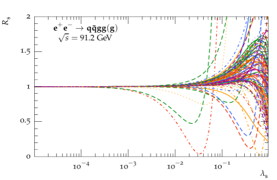
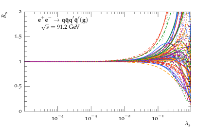
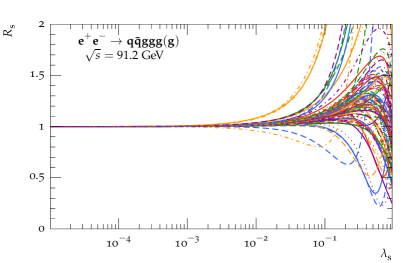
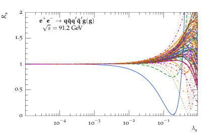
Figure 1: Ratio of the eikonal approximation to the exact $e^{+}e^{-}\to 5-,6-\mathrm{parton}$ tree-level matrix element versus the softness parameter $\lambda_{\text{s}}$.

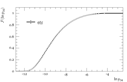
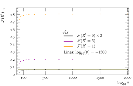
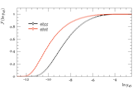
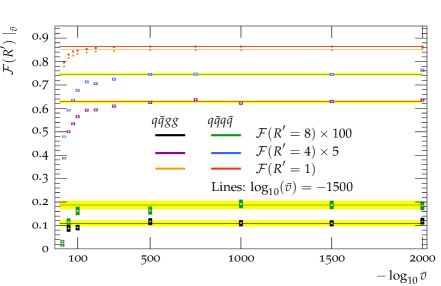
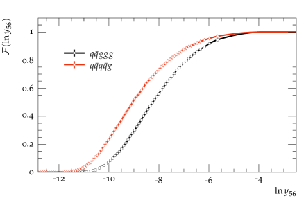
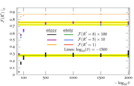
Figure 2: Multiple-emission function $\mathcal{F}$ for the different Born channels $\delta$ appearing in the resummation of $y_{34}$, $y_{45}$, and $y_{56}$, respectively. While the left column emphasises the dependence on the large logarithm, i.e., $\ln(y_{n,n+1})$, the right column shows the convergence of the numerical evaluation of the limit $\bar{v}\to 0$ for selected values of $R^{\prime}$. The lines with error bands mark the value and statistical uncertainty for $\bar{v}=10^{-1500}$. Note that for $y_{34}$ as well as the other $\mathcal{F}$ functions with $R^{\prime}=1$, the dot sizes are larger than the error bar would be.

Validation and results for the multiple-emission function

The $\mathcal{F}$ function is evaluated numerically for all relevant multiplicities and, where needed, different channels $\delta$. In the limit $\bar{v}\rightarrow 0$, all emissions become collinear to their hard legs and emissions are only clustered together if they originate from the same parton in the Born event. From this, it is straight-forward to see that the multiple-emission function is independent of details of the Born kinematics and can thus be evaluated for a reference configuration for each flavour channel $\delta$. This amounts to calculate $\mathcal{F}$ for every possible number of external gluons. Applying the condition of emissions being only clustered if they were emitted from the same Born parton explicitly removes any dependence on the used kinematics.

For reference, the numerical results for $\mathcal{F}(L)$ are shown in Fig. 2, for a configuration with $\mu_{R}^{2}=\mu_{Q}^{2}=y_{\mathrm{cut}}Q^{2}$. This could be converted to $\mathcal{F}(R^{\prime})$ using Eq. (31). In the same figure, we also show how $\mathcal{F}(R^{\prime})$ approaches the $\bar{v}\to 0$ limit for several representative $R^{\prime}$ values. It is not feasible to stick to double precision such that multiple-precision arithmetics have to be used. However we are observing convergence starting from values of $\bar{v}\approx 10^{-500}$. It appears that, when interpreted as a function of $R^{\prime}$, the dependence of $\mathcal{F}$ on the Born channel is almost insignificant, in particular for $y_{56}$. Note, however, that the two functions are not exactly equal in any case and that this similarity depends on the relatively close numerical values of the Casimirs $C_{\text{F}}$ and $C_{\text{A}}$.

In the numerical evaluation of Eq. (12), the limits of the soft scaling $\bar{v}\to 0$, the cutoff $\epsilon\to 0$, and the number points used in the Monte Carlo integration $N_{\mathrm{points}}\to\infty$ are taken numerically, thus replacing $0$ ($\infty$) with a very small (large) but finite value. Finite Monte Carlo statistics limit the numerical accuracy of the integral evaluation, while subleading contributions are introduced for non-zero $\bar{v}$ and $\epsilon$. This causes a systematic difference with respect to taking the exact limit as done for instance for the $y_{23}$ resolution scale in Ref. [12]. Although, one could imagine implementing the algorithm used there for higher parton multiplicities to avoid any subleading contributions, we opt for a fully generic approach here. We argue that subleading contributions can be controlled to an extent that they become insignificant in final results. However, given that smaller values of $\bar{v}$ and $\epsilon$ increase the computation time per Monte Carlo point, a compromise between eliminating subleading contributions and the number of points $N_{\mathrm{points}}$ we can reasonably evaluate given the computing resources available needs to be found. In the right-hand panel of Fig. 2, we demonstrate that, indeed, for sufficiently small $\bar{v}$ values $\mathcal{F}$ reaches a plateau and no longer significantly depends on the very value of $\bar{v}$. The remaining subleading contributions are of order of the statistical precision used to check the residual dependence of $\mathcal{F}$. At the same time, we verify that the remaining statistical uncertainty of the Monte Carlo evaluation of $\mathcal{F}$ is insignificant for our final resummed prediction.

To validate our procedure, we compare our default approach to evaluate $\mathcal{F}$ with the algorithm described in [12] for the specific case of the observable $y_{23}$. We use our default set of numerical parameters and compare the two algorithms in the left panel of Fig. 3, observing that they indeed approach the same values. The remaining differences are of the same order of magnitude as the statistical uncertainty. Given our target statistical accuracy for $\mathcal{F}$ of order 1% subleading terms here do indeed not exceed the 2% level.

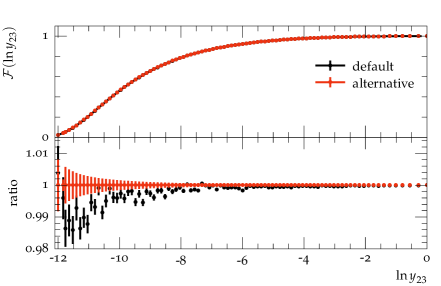
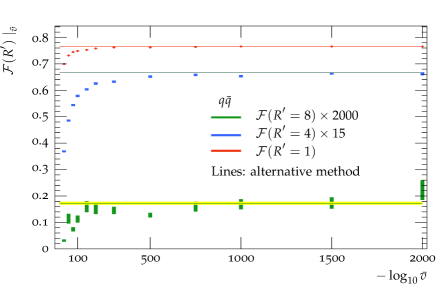
Figure 3: Multiple-emission function $\mathcal{F}$ appearing in the resummation of $y_{23}$, evaluated with our default numerical algorithm and the alternative method described in [12]. The left panel presents the dependence on the large logarithm, i.e., $\ln(y_{23})$, the right panel shows the convergence of the numerical evaluation in the limit $\bar{v}\to 0$ for selected values of $R^{\prime}$. The lines with error bands mark the value and statistical uncertainty when using the exact NLL algorithm presented in [12].

To match to NLO fixed-order distributions, we also need the expansion of $\mathcal{F}$. The argument of [12] applies to higher multiplicities, and we can generally write

$$\mathcal{F}=1+\sum_{p=2}^{\infty}\mathcal{F}_{p}R^{\prime p}~{},\hskip 28.45274pt\mathcal{F}_{2}=-\frac{\pi^{2}}{8}\frac{\sum_{l\in\delta}C_{l}^{2}}{2\left(\sum_{l\in\delta}C_{l}\right)^{2}}\,.$$ (29)

Numerically, we checked that these values are correctly reproduced in the corresponding integrals, again validating the limit.

4 Predictions for Durham jet-resolution scales

In this section, we present our results for the $4-$, $5-$, and $6-$jet Durham resolution scales. Our central results, the resummed predictions to $\mathrm{NLO+NLL}^{\prime}$ accuracy, are presented in Sec. 4.1; we study the influence of LO and NLO matching as well as subleading colour contributions in Sec. 4.2 and Sec. 4.3, respectively; in Sec. 4.4, we then compare the resummed predictions with parton-shower simulations from SHERPA and VINCIA, where we also address the impact of hadronisation corrections on the parton-level distributions.

4.1 Resummed predictions for multijet resolutions

Our central results are the resummed distributions of the Durham jet resolutions $y_{34}$, $y_{45}$, and $y_{56}$, in the definition discussed in Sec. 3.1. In particular, we require the Born events to possess $n=3,4,5$ jets separated by at least $y_{\mathrm{cut}}=0.02$ in the calculation for $y_{n,n+1}$, respectively. We perform our calculation at the LEP1 centre-of-mass energy $\sqrt{s}=91.2~{}\mathrm{GeV}$. We use the LogR matching scheme as described in Sec. 2.3 to obtain physical distributions over the full range of the observable. Fig. 4 shows our predictions at LO and NLO, matched to NLL by the means of the preceding sections to achieve an accuracy of $\mathrm{LO+NLL}^{\prime}$ and $\mathrm{NLO+NLL}^{\prime}$, respectively. To estimate theoretical uncertainties from missing higher-order corrections, we consider independent variations of $\mu_{R}$ , $\mu_{Q}$, and $p$ by factors of $0.5$ and $2$, resulting in the yellow ($\mathrm{LO+NLL}^{\prime}$) and orange ($\mathrm{NLO+NLL}^{\prime}$) bands.

For higher jet multiplicities, we observe a narrowing of the distributions as well as a growing impact of NLO contributions compared to the LO result, being significant only for $y_{45}$ and $y_{56}$. In the peak region, the impact of NLO corrections stays rather small in any case, being of order of a few percent only. Regarding $y_{34}$, the NLO corrections do not have a large impact on the central prediction, we do, however, observe a considerable reduction of the theoretical uncertainties, at least away from the very soft region, where higher-logarithmic corrections become significant. This expected reduction of uncertainties is observed for the higher multiplicities as well. Here, the impact of NLO corrections on the matched distributions become larger when approaching the kinematic endpoint, $y_{n,n+1}\approx y_{\mathrm{kin}}$, but consistently stay within the LO uncertainty band.

The remaining statistical uncertainty from the numerical determination of the $\mathcal{F}$-function is propagated through to the final result, indicated by the error bars on the $\mathrm{NLO+NLL}^{\prime}$ prediction. It is entirely negligible compared to the overall uncertainty from scale variations. In light of our earlier discussion of subleading effects emerging from taking the limits in the evaluation of $\mathcal{F}$ numerically, we conclude that these are indeed insignificant for our final predictions.

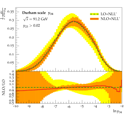
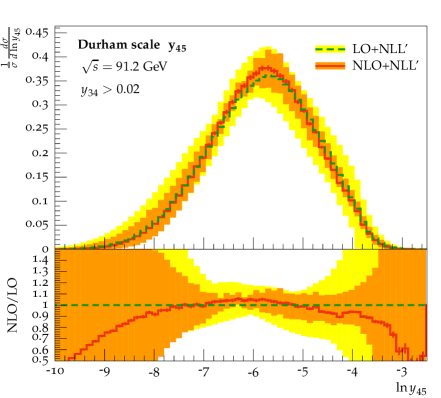
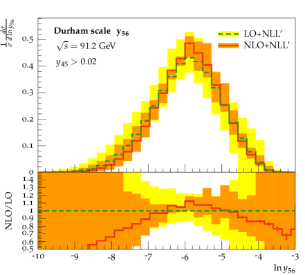
Figure 4: Resummed predictions for the Durham jet-resolutions $y_{34}$, $y_{45}$, and $y_{56}$ in electron-positron annihilation at $\sqrt{s}=91.2$ GeV. The lower panels show the local NLO K-factor.

4.2 Impact of fixed-order corrections

In Fig. 5, we compare the fixed-order predictions to the expansion obtained from the resummed results for the three observables $y_{34}$, $y_{45}$, and $y_{56}$. We explicitly check their asymptotic agreement in the limit $y_{n,n+1}\to 0$. As expected, the difference between fixed order and the expansion of the resummed distribution approaches zero in the soft limit. In the expansion $\Sigma^{(2)}$, there are missing terms of order $\alpha_{\text{s}}^{(n-2)}\alpha_{\text{s}}^{2}L^{2}$ and $\alpha_{\text{s}}^{(n-2)}\alpha_{\text{s}}^{2}L$ that are present in the fixed-order NLO calculation. Hence, we have a mismatch between fixed-order calculation and expansion which, in the differential distribution, is growing linearly in $L$, see the orange line in Fig. 5. After including the $\frac{\alpha_{\text{s}}}{2\pi}C_{1}^{\delta}$ coefficients, which effectively happens in the matching, only missing terms of order $\alpha_{\text{s}}^{(n-2)}\alpha_{\text{s}}^{2}L$ remain. These are subleading with respect to the $\mathrm{NLL}^{\prime}$ resummation, although leading to a constant but finite difference in the differential distributions between fixed order and expansion. This is also demonstrated in Fig. 5, where in the purple line we include the respective matching coefficient as it would effectively appear in the multiplicative matching. As the NLO calcuation is computationally expensive, we do not attempt to carry it out at sufficient precision to allow for an extraction of the actual constant. Note that the matching schemes in Sec. 2.3 are designed such that the matched distributions behave in a physically meaningful way, i.e., are driven to zero by the resummed distribution, cf. Fig. 4, requiring a much less precise calculation in the soft tail of the fixed-order correction. We compared our results presented in the previous section to the ones obtained in the multiplicative matching scheme, but did not find significant differences, except for the region $y_{n,n+1}>y_{\mathrm{cut}}$. There, however, scale uncertainties also become very large, such that the difference between the two matching schemes is always covered by the NLO scale variation in the LogR matching scheme. We thus do not include an explicit uncertainty related to the matching scheme.

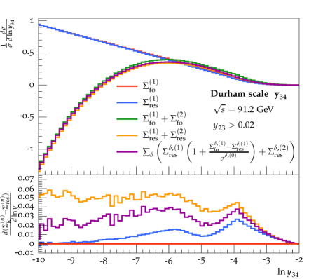
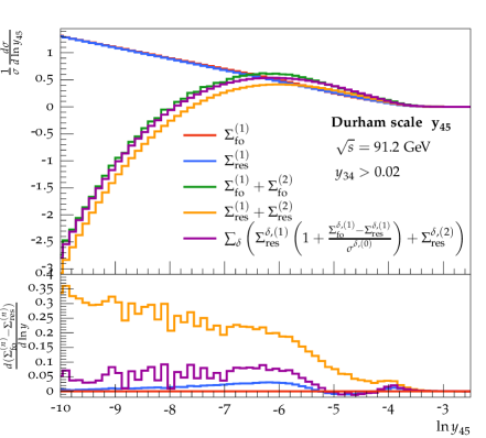
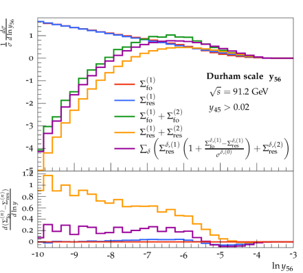
Figure 5: Fixed-order predictions for $y_{34}$, $y_{45}$, and $y_{56}$. We show the expansion of $\Sigma_{\mathrm{res}}$ to the relevant orders, and the expansion to second order including the expression approaching the $C_{1}$ coefficient in the soft limit. The lower panels show the total difference between fixed order and expansion.

4.3 Impact of subleading colour contributions

Our results enable us to quantify the impact of subleading colour corrections on multijet observables. This is of particular interest for example in the context of recent and ongoing developments to systematically include such corrections into parton-shower event generators, see e.g. [48, 49, 50, 51, 52, 53, 54, 55, 56]. To assess the effect of subleading colour contributions, we redo our calculation in the t’Hooft large-$N_{\text{C}}$ limit, defined by taking $N_{\text{C}}\to\infty$ while keeping $\alpha_{\text{s}}N_{\text{C}}$ fixed [57]. This approximation, to which we will refer to as leading colour (LC), has a significant impact on the various contributions in Eq. (2). Firstly, all Casimirs corresponding to different legs are simplified to $N_{\text{C}}=2C_{\text{F}}=C_{\text{A}}$. Secondly, quark-loop contributions become negligible in both, the anomalous dimensions and the beta function. Finally, all non-planar diagrams vanish, leading to a simplification of colour-insertion operators. As the latter is only relevant to the colour-correlation contribution $\mathcal{S}$, we define an ”improved large-$N_{\text{C}}$” approximation (imp. LC), in which we only treat the colour correlators appearing in $\Gamma$, and hence $\mathcal{S}$, in the strict $N_{\text{C}}\to\infty$ limit, while still including the correct subleading contributions in $R_{l}$ and $\mathcal{F}$. Those have a clear interpretation as sums over contributions from individual legs, such that the proper leg-specific $\mathrm{SU(3)}$ Casimir operators can be assigned. As in our main calculation, we match both resulting resummed distributions to the full-colour NLO result in the LogR scheme. The results of this study are presented in Fig. 6 and we collect details on the analytical treatment of subleading colour contributions in App. A.

While there is a significant impact on the distributions when taking the t’Hooft large-$N_{\text{C}}$ limit, it is negligible for the improved large-$N_{\text{C}}$ limit, although in both cases, the results stay entirely within the uncertainty band of the $\mathrm{NLO+NLL}^{\prime}$ prediction. Moreover, in the peak region there is almost no difference between the full-colour and the improved large-$N_{\text{C}}$ result; the only visible difference being in the soft-tail region, where, however, the effect is below $5\%$ for $y_{34}$ and $y_{45}$ and only sizeable in the ultra-soft region of $y_{56}$.

To ease the interpretation of these results in the context of subleading colour corrections in parton showers, which so far in the literature have mostly been discussed in the context of pure, unmatched showers, we show the ratios between full, improved, and leading-colour approximation at NLL, $\text{LO}+\text{NLL}^{\prime}$, and $\text{NLO}+\text{NLL}^{\prime}$ accuracy in Fig. 6. It is evident that the effect of subleading colour contributions is largely captured by the matching, which is expected as we include the full colour information in the fixed-order calculations. Without any matching, we find the corrections to the improved leading-colour scheme to be compatible with the naive expectation that, away from the kinematical extreme regions, subleading colour contributions are suppressed by $1/N_{\text{C}}^{2}\approx 10\%$. Already LO matching allows for a significant reduction of these effects. We remark, however, that a direct interpretation of these observations in the context of full-colour parton showers is still not straight forward, as the matching involves an intricate interleave of subleading colour and kinematical corrections. It is, however, reasonable to argue that subleading colour effects are rather small and anyway overwhelmed by the fixed-order corrections. At least for the observables considered here, there is virtually no difference between the calculations at full-colour and in the improved large-$N_{\text{C}}$ limit, as long as both are matched to exact, full-colour matrix elements.

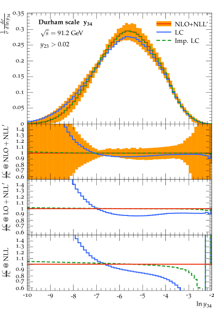
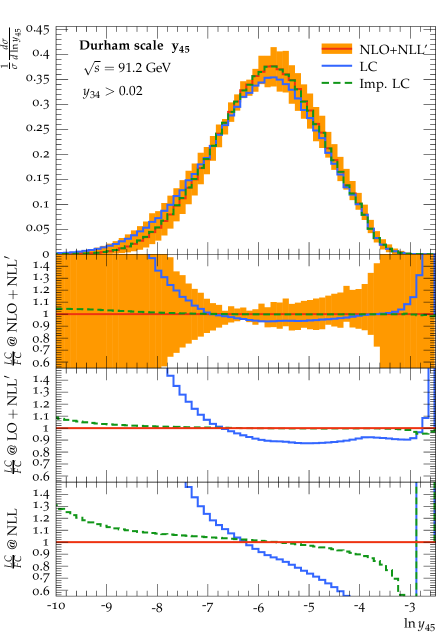
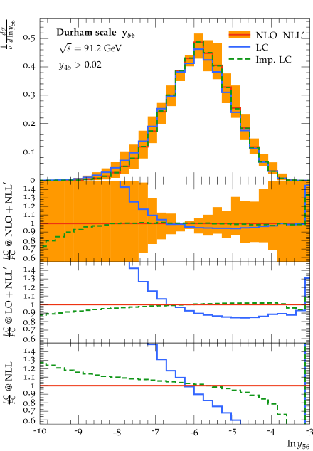
Figure 6: Durham splitting scales $y_{n,n+1}$ at $\mathrm{NLO+NLL}^{\prime}$ accuracy, in the $N_{\text{C}}\to\infty$ limit, and in the improved LC scheme. The lower panels show the corresponding ratios additionally at $\mathrm{LO+NLL}^{\prime}$ accuracy and for the resummation without any matching.

4.4 Comparison to parton-shower predictions

Our resummed $\mathrm{NLO+NLL}^{\prime}$ predictions for the Durham jet resolutions provide highly non-trivial benchmarks for corresponding predictions from QCD Monte-Carlo event generators. They allow to gauge the results from parton-shower simulations and the methods used to combine these with exact higher-order QCD matrix elements and might guide the way to further improving showering algorithms. On the other hand, Monte-Carlo simulations provide means to include non-perturbative corrections from the parton-to-hadron transition, that ultimately need to be taken into account for a realistic comparison with experimental data.

As a first step in this direction we compare our resummed results against predictions from two distinct parton-shower implementations: the dipole parton shower css [58] as implemented in the SHERPA event generator and the VINCIA 1 antenna-shower plug-in [59] to the PYTHIA 8 event generator [60]. In Fig. 7 we present our results obtained using matrix-element plus parton-shower simulations at parton level for $y_{34}$, $y_{45}$, and $y_{56}$ in comparison to the $\mathrm{NLO+NLL}^{\prime}$ predictions. Furthermore, in the right panels of Fig. 7 we present hadron-level predictions, compared to the respective parton-level results.

To account for the kinematics and colour correlations of the respective Born processes, both showers are corrected to exact LO and NLO calculations, using two different strategies. One the one hand, in SHERPA we consider an MEPS@LO [61] calculation with exact tree-level matrix elements for $e^{+}e^{-}\to 2,3,4,5$ final-state partons. We also compare to a calculation using the MEPS@NLO merging strategy [62], including one-loop QCD corrections for $e^{+}e^{-}\to 2,3,4$ partons via the MC@NLO method [63, 64] as implemented in SHERPA and $e^{+}e^{-}\to 5$ partons at tree level. We again make use of the matrix-element generator COMIX, and use OpenLoops to compute the virtual corrections. The merging parameter is set to $y_{\textrm{cut}}=\left(Q_{\textrm{cut}}/E_{\textrm{CMS}}\right)^{2}=10^{-2}$ for the both the MEPS@LO and the MEPS@NLO calculation. The VINCIA antenna shower, on the other hand, is matched to $e^{+}e^{-}\to 2,3$ matrix elements at one-loop level as presented in [65] and $e^{+}e^{-}\to 4,5,6$ tree-level matrix elements obtained from the MADGRAPH 4 matrix-element generator [66] via matrix-element corrections in the unitary GKS formalism [67]. Matrix-element corrections for $5-$ and $6-$ parton processes are smoothly regularised at a matching scale of $Q_{\text{match}}/E_{\text{CMS}}=0.05$. For comparability, we restrict the phase space to strongly ordered branchings only. In both showers, the strong coupling is evolved at two-loop order in the CMW scheme, assuming an $\overline{\text{MS}}$ value of $\alpha_{\text{s}}(m_{Z}^{2})=0.118$.

We observe that the MEPS@LO and VINCIA samples agree well with each other and are close to the analytic calculation in the peak region as well as in the hard region, apart from the immediate neighbourhood of the endpoint. The MEPS@NLO sample is generally not improving the agreement between analytic and parton-shower prediction. In fact for $y_{34}$ and $y_{45}$ it yields somewhat larger deviations. However, we do not determine an explicit uncertainty estimate for the Monte Carlo predictions here, but their size can be considered similar to those of the analytic calculation. Accordingly, all the presented predictions are indeed in very good agreement. Comparing to our results in the previous section, the effects of subleading colour contributions are qualitatively different and smaller than the differences we observe between our resummed results and the parton-shower predictions. Apparently, for the particular observable definition we consider here, missing subleading colour contributions are not driving these differences but rather ambiguities related to recoil schemes, phase-space constraints and the treatment of subleading contributions in the running of $\alpha_{\text{s}}$, see for example Refs. [68, 69, 70].

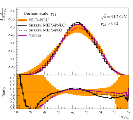
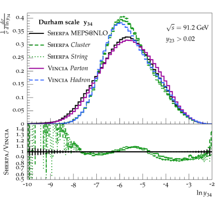
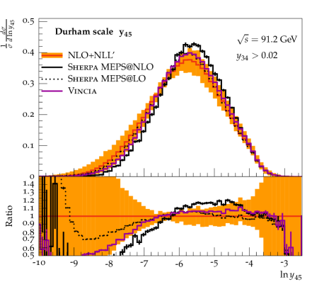
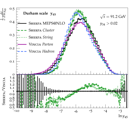
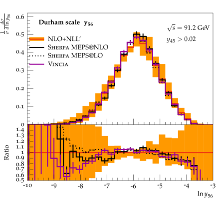
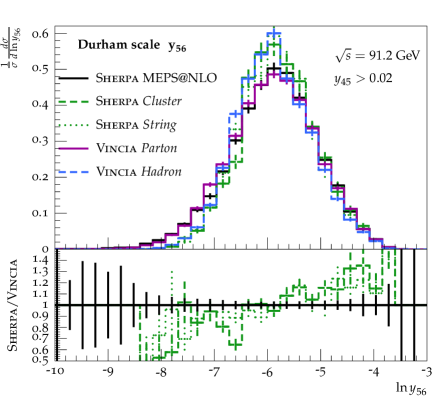
Figure 7: Comparison of resummed $\mathrm{NLO+NLL}^{\prime}$ predictions for $y_{34}$, $y_{45}$, and $y_{56}$ to parton-level parton-shower simulations from SHERPA and VINCIA (left column). The right column compiles corresponding hadron-level results. The shower results from VINCIA are hadronised with the Lund string model in PYTHIA 8. For the css, the SHERPA implementation of the Cluster model is used (dashed line) as well as the Lund model from PYTHIA 6 (dotted line). The hadronisation corrections from SHERPA are all based on the MEPS@NLO sample.

As our observable definition differs from the usual experimental definition of jet-resolution scales by the hard cut we impose on the Born event, we need to gauge the influence of the parton-to-hadron transition on this observable. To this end we compare generator predictions on parton and hadron level. For SHERPA, we invoke SHERPA’s default hadronisation model, based on cluster fragmentation [71] and furthermore, hadronise SHERPA’s parton-level events with the Lund string fragmentation [72] as implemented in PYTHIA 6.4 [73]. Parton-level predictions of the VINCIA antenna shower are hadronised using the Lund string model in PYTHIA 8.2.

We obtain sizeable hadronisation corrections in all multiplicities. Their impact is very similar for the cluster- and string-fragmentation model applied to SHERPA’s parton-level results. A qualitatively similar effect can be seen in the string hadronisation of VINCIA’s parton-level results. In all cases, the soft tail of the distributions is significantly suppressed, leading to a narrowing of the distribution and hence a more pronounced peak. Reassuringly, the hard tail is only mildly affected by either of the fragmentation models. Quantitatively, however, there are differences of up to $10-20\%$ remaining between the hadron-level predictions from SHERPA and VINCIA in the central peak region. We note that this is largely compatible with the deviations seen in the comparison at parton level. As the two predictions from SHERPA with different hadronisation models agree relatively well, it can be expected that generic non-perturbative uncertainties are rather moderate. Moreover, taking into account that we do not include uncertainties regarding the variation of hadronisation parameters, all hadron-level predictions agree reasonably well with each other.

5 Conclusions

For the first time, we have here obtained resummed predictions at $\mathrm{NLO+NLL}^{\prime}$ accuracy for multijet resolution scales in electron-positron annihilation. We employ the CAESAR formalism in a largely automated manner within the SHERPA event-generator framework. All relevant colour spaces were decomposed over the trace basis to obtain hard-scattering matrix elements and colour correlators that account for the insertion of soft-gluon radiation. Both, the construction of the basis and the calculation of colour insertions, have been performed in an automated way. Multijet matrix elements are obtained from the COMIX matrix-element generator, that is part of SHERPA. For NLO QCD predictions we obtain virtual corrections for $e^{+}e^{-}\to 3,4,5$ partons from OpenLoops, while using Recola for virtual corrections to $e^{+}e^{-}\to 6$ partons. For the evaluation of the multiple-emission contribution, represented by the $\mathcal{F}$-function in the CAESAR formalism, we resort to a numerical evaluation using multiple-precision arithmetics.

We have derived predictions for the Durham jet-resolution scales $y_{34}$, $y_{45}$, and $y_{56}$ at $\mathrm{NLO+NLL}^{\prime}$ accuracy, using a Durham resolution $y_{\mathrm{cut}}=0.02$ to restrict the respective Born configurations to sufficiently hard kinematics. The inclusion of NLO QCD corrections significantly reduces the theoretical uncertainties, estimated via scale variations.

We studied the impact of subleading colour contributions to our predictions, by repeating our calculations in the LC as well as the improved LC scheme, which we regard as being similar to the colour treatment in parton showers. We observe significant differences to the full-colour prediction only in the (strict) LC limit, while already at NLL the improved LC scheme well approximates the full-colour prediction. At $\mathrm{NLO+NLL}^{\prime}$ accuracy, we observe virtually no difference between the improved LC and the full-colour result.

As a benchmark for parton showers and an estimate of non-perturbative effects on the observable, we compared our resummed predictions against two distinctly different parton-shower algorithms, the VINCIA antenna shower plug-in to PYTHIA and the Catani–Seymour dipole shower in SHERPA, matched to LO and NLO. We observe good agreement between the VINCIA and MEPS@LO as well as the MEPS@NLO results. The found effects of subleading colour contributions are qualitatively different and smaller than the differences observed when comparing resummed results and parton-shower predictions. Apparently these will rather originate from ambiguities related to recoil schemes, phase-space constraints and the treatment of subleading contributions in the running of $\alpha_{\text{s}}$ in the parton-shower implementations. The effect of non-perturbative corrections was studied by including hadronisation effects for the VINCIA and SHERPA parton showers, employing both, cluster and string fragmentation for the latter. We found good agreement between all hadron-level results. The observed deviations between SHERPA and VINCIA can already be found at the parton level. This confirms the suitability of jet-resolution scales for studies of perturbative QCD dynamics.

A direct comparison of our predictions to existing LEP measurements of jet resolutions is not straight-forward, due to the required regularisation of the multijet Born processes. A corresponding reanalysis of LEP data would be desirable. To be able to compare to existing $e^{+}e^{-}$ data, more general hierarchies of the multi-scale problem need to be addressed. By the generality of the approach presented here, our study may be extended to $k_{T}$ jet-resolution scales in hadronic collisions, motivating dedicated measurements at the LHC.

Appendix A Analytic expressions

For completeness, we here collect all analytic expressions of the CAESAR formalism that did not appear in the main text, restricted to the jet-resolution scales studied here and our conventions. In particular, we choose to rescale the arguments of all logs with $x_{v}=d(\mu_{Q})$, so that no explicit dependence on $d$ appears. We use the short-hand $\lambda=\alpha_{\text{s}}(\mu_{R}^{2})\beta_{0}L$, and fix the normalisation of colour operators to $T_{\text{R}}=1/2$, resulting in $C_{l}=C_{\text{A}}=N_{\text{C}}$ for gluons and $C_{l}=C_{\text{F}}=(N_{\text{C}}-1/N_{\text{C}})/2$ for quarks. The radiator of leg $l$ is given by

$$\begin{split}R_{l}(L)&=-\frac{C_{l}}{2\pi\beta_{0}}\left[L\left(1+\frac{\ln(1-\lambda)}{\alpha_{\text{s}}\beta_{0}}\right)\right.-\left(2B_{l}+\ln\frac{Q^{2}}{\mu_{Q}^{2}}\right)\ln(1-\lambda)\\ &\left.+\left(\frac{K}{2\pi\beta_{0}}+\ln\frac{\mu_{R}^{2}}{\mu_{Q}^{2}}\right)\left(\ln(1-\lambda)+\frac{\lambda}{1-\lambda}\right)+\frac{\beta_{1}}{\beta_{0}^{2}}\left(\frac{1}{2}\ln^{2}(1-\lambda)+\frac{\ln(1-\lambda)+\lambda}{1-\lambda}\right)\right]\,.\end{split}$$ (30)

Its derivative with respect to $L$ is single logarithmic,

$$R^{\prime}_{l}=\frac{C_{l}}{2\pi\beta_{0}}\frac{\lambda}{1-\lambda}.$$ (31)

We also use the shorthands $R=\sum_{l}R_{l}$, $R^{\prime}=\sum_{l}R^{\prime}_{l}$ where this eases the notation. The usual constants in the $\overline{\text{MS}}$ scheme are

$$\begin{split}\beta_{0}&=\frac{11C_{\text{A}}-2n_{\text{f}}}{12\pi}\,,~{}&\beta_{1}&=\frac{17C_{\text{A}}^{2}-5C_{\text{A}}n_{\text{f}}-3C_{\text{F}}n_{\text{f}}}{24\pi^{2}}\,,\\ K&=C_{\text{A}}\left(\frac{67}{18}-\frac{\pi^{2}}{6}\right)-\frac{5}{9}n_{\text{f}}\,,~{}&B_{q}&=-\frac{3}{4},~{}&B_{g}&=-\frac{\pi\beta_{0}}{C_{\text{A}}}\,,\end{split}$$ (32)

where we have already employed our normalisation convention. In the t’Hooft limit, $N_{\text{C}}\to\infty$ with $\alpha_{\text{s}}N_{\text{C}}=\alpha_{\text{s},0}=\mathrm{const.}$, all expressions depend only on the finite quantities

$$\begin{split}\frac{C_{\text{F}}}{2\pi\beta_{0}}&\to\frac{3}{11}\,,~{}&\frac{C_{\text{A}}}{2\pi\beta_{0}}&\to\frac{6}{11}\,,~{}&\alpha_{\text{s}}\beta_{0}&\to\frac{11}{12\pi}\alpha_{\text{s},0}\,,\\ \frac{K}{2\pi\beta_{0}}&\to\frac{67/3-\pi^{2}}{11}\,,~{}&\frac{\beta_{1}}{\beta_{0}^{2}}&\to\frac{102}{121}\,.\end{split}$$ (33)

When working in the large-$N_{\text{C}}$ limit, the $\mathcal{F}$ function needs to be re-evaluated in principle. However, it only depends on the ratios of sums of Casimirs for the different legs and on $R^{\prime}$. Thus only the configurations with mixed quark and gluon content need to be re-computed with $C_{\text{A}}/C_{\text{F}}=2$.

When evaluating colour correlators in the large-$N_{\text{C}}$ limit, we are interested in

$$\alpha_{\text{s}}\frac{\bra{b_{\alpha}}\boldsymbol{T}_{i}\boldsymbol{T}_{j}\ket{b_{\beta}}}{|b_{\alpha}||b_{\beta}|}\to\alpha_{\text{s},0}\bra{b_{\alpha}}\boldsymbol{T}_{i}\boldsymbol{T}_{j}\ket{b_{\beta}}_{\mathrm{LNC}}\,,\hskip 28.45274pt\bra{b_{\alpha}}\boldsymbol{T}_{i}\boldsymbol{T}_{j}\ket{b_{\beta}}_{\mathrm{LNC}}=\lim_{N_{\text{C}}\to\infty}\frac{\bra{b_{\alpha}}\boldsymbol{T}_{i}\boldsymbol{T}_{j}\ket{b_{\beta}}}{N_{\text{C}}|b_{\alpha}||b_{\beta}|}\,.$$ (34)

Note that we need to normalise the basis vectors in order to obtain a finite result. As expected, the $\bra{b_{\alpha}}\boldsymbol{T}_{i}\boldsymbol{T}_{j}\ket{b_{\beta}}_{\mathrm{LNC}}$ correlators vanish for all non-planar diagrams and give finite contributions otherwise. Practically, we calculate the large-$N_{\text{C}}$ colour correlators by comparing the powers of $N_{\text{C}}$ in the numerator and denominator of Eq. (34) and keeping only those with the same highest power. This modification of the colour correlators is the only one that is still present in the improved LC scheme.

References

- [1] S. Catani, Y. L. Dokshitzer, M. Olsson, G. Turnock and B. R. Webber, New clustering algorithm for multi - jet cross-sections in e+ e- annihilation, Phys. Lett. B269 (1991), 432–438
- [2] S. Catani, L. Trentadue, G. Turnock and B. R. Webber, Resummation of large logarithms in event shape distributions, Nucl. Phys. B407 (1993), 3–42
- [3] A. Banfi, G. Marchesini, Y. L. Dokshitzer and G. Zanderighi, QCD analysis of near-to-planar three jet events, JHEP 07 (2000), 002, [arXiv:hep-ph/0004027 [hep-ph]]
- [4] M. D. Schwartz, Resummation and NLO matching of event shapes with effective field theory, Phys. Rev. D77 (2008), 014026, [arXiv:0709.2709 [hep-ph]]
- [5] T. Becher and M. D. Schwartz, A precise determination of from LEP thrust data using effective field theory, JHEP 07 (2008), 034, [arXiv:0803.0342 [hep-ph]]
- [6] R. Abbate, M. Fickinger, A. H. Hoang, V. Mateu and I. W. Stewart, Thrust at N3LL with Power Corrections and a Precision Global Fit for alphas(mZ), Phys. Rev. D83 (2011), 074021, [arXiv:1006.3080 [hep-ph]]
- [7] P. F. Monni, T. Gehrmann and G. Luisoni, Two-Loop Soft Corrections and Resummation of the Thrust Distribution in the Dijet Region, JHEP 08 (2011), 010, [arXiv:1105.4560 [hep-ph]]
- [8] T. Becher and G. Bell, NNLL Resummation for Jet Broadening, JHEP 11 (2012), 126, [arXiv:1210.0580 [hep-ph]]
- [9] R. Abbate, M. Fickinger, A. H. Hoang, V. Mateu and I. W. Stewart, Precision Thrust Cumulant Moments at LL, Phys. Rev. D86 (2012), 094002, [arXiv:1204.5746 [hep-ph]]
- [10] A. J. Larkoski, D. Neill and J. Thaler, Jet Shapes with the Broadening Axis, JHEP 04 (2014), 017, [arXiv:1401.2158 [hep-ph]]
- [11] A. Banfi, H. McAslan, P. F. Monni and G. Zanderighi, A general method for the resummation of event-shape distributions in annihilation, JHEP 05 (2015), 102, [arXiv:1412.2126 [hep-ph]]
- [12] A. Banfi, G. P. Salam and G. Zanderighi, Semi-numerical resummation of event shapes, JHEP 01 (2002), 018, [arXiv:hep-ph/0112156 [hep-ph]]
- [13] A. Banfi, H. McAslan, P. F. Monni and G. Zanderighi, The two-jet rate in at next-to-next-to-leading-logarithmic order, Phys. Rev. Lett. 117 (2016), no. 17, 172001, [arXiv:1607.03111 [hep-ph]]
- [14] G. Dissertori, A. Gehrmann-De Ridder, T. Gehrmann, E. W. N. Glover, G. Heinrich and H. Stenzel, Precise determination of the strong coupling constant at NNLO in QCD from the three-jet rate in electron–positron annihilation at LEP, Phys. Rev. Lett. 104 (2010), 072002, [arXiv:0910.4283 [hep-ph]]
- [15] S. Bethke, S. Kluth, C. Pahl and J. Schieck, The JADE collaboration, Determination of the Strong Coupling alpha(s) from hadronic Event Shapes with O(alpha**3(s)) and resummed QCD predictions using JADE Data, Eur. Phys. J. C64 (2009), 351–360, [arXiv:0810.1389 [hep-ex]]
- [16] G. Dissertori, A. Gehrmann-De Ridder, T. Gehrmann, E. W. N. Glover, G. Heinrich, G. Luisoni and H. Stenzel, Determination of the strong coupling constant using matched NNLO+NLLA predictions for hadronic event shapes in annihilations, JHEP 08 (2009), 036, [arXiv:0906.3436 [hep-ph]]
- [17] A. Verbytskyi, A. Banfi, A. Kardos, P. F. Monni, S. Kluth, G. Somogyi, Z. Szőr, Z. Trøcsányi, Z. Tulipánt and G. Zanderighi, High precision determination of from a global fit of jet rates, JHEP 08 (2019), 129, [arXiv:1902.08158 [hep-ph]]
- [18] E. Gerwick, S. Schumann, B. Gripaios and B. Webber, QCD Jet Rates with the Inclusive Generalized kt Algorithms, JHEP 04 (2013), 089, [arXiv:1212.5235 [hep-ph]]
- [19] M. Cacciari, G. P. Salam and G. Soyez, FastJet User Manual, Eur. Phys. J. C72 (2012), 1896, [arXiv:1111.6097 [hep-ph]]
- [20] B. R. Webber, QCD Jets and Parton Showers, Quantum chromodynamics and beyond: Gribov-80 memorial volume. Proceedings, Memorial Workshop devoted to the 80th birthday of V.N. Gribov, Trieste, Italy, May 26-28, 2010, 2011, pp. 82–92
- [21] A. Heister et al., The ALEPH collaboration, Studies of QCD at e+ e- centre-of-mass energies between 91-GeV and 209-GeV, Eur. Phys. J. C35 (2004), 457–486
- [22] G. Abbiendi et al., The OPAL collaboration, Measurement of event shape distributions and moments in hadrons at 91-GeV - 209-GeV and a determination of alpha(s), Eur. Phys. J. C40 (2005), 287–316, [arXiv:hep-ex/0503051 [hep-ex]]
- [23] A. Buckley et al., General-purpose event generators for LHC physics, Phys. Rept. 504 (2011), 145–233, [arXiv:1101.2599 [hep-ph]]
- [24] A. Banfi, G. P. Salam and G. Zanderighi, Generalized resummation of QCD final state observables, Phys. Lett. B584 (2004), 298–305, [arXiv:hep-ph/0304148 [hep-ph]]
- [25] A. Banfi, G. P. Salam and G. Zanderighi, Principles of general final-state resummation and automated implementation, JHEP 03 (2005), 073, [arXiv:hep-ph/0407286 [hep-ph]]
- [26] T. Gleisberg, S. Höche, F. Krauss, M. Schönherr, S. Schumann, F. Siegert and J. Winter, Event generation with SHERPA 1.1, JHEP 02 (2009), 007, [arXiv:0811.4622 [hep-ph]]
- [27] E. Bothmann et al., Event Generation with Sherpa 2.2, SciPost Phys. 7 (2019), no. 3, 034, [arXiv:1905.09127 [hep-ph]]
- [28] E. Gerwick, S. Höche, S. Marzani and S. Schumann, Soft evolution of multi-jet final states, JHEP 02 (2015), 106, [arXiv:1411.7325 [hep-ph]]
- [29] S. Marzani, D. Reichelt, S. Schumann, G. Soyez and V. Theeuwes, Fitting the Strong Coupling Constant with Soft-Drop Thrust, JHEP 11 (2019), 179, [arXiv:1906.10504 [hep-ph]]
- [30] A. Banfi, G. P. Salam and G. Zanderighi, Resummed event shapes at hadron - hadron colliders, JHEP 08 (2004), 062, [arXiv:hep-ph/0407287 [hep-ph]]
- [31] A. Banfi, G. P. Salam and G. Zanderighi, Phenomenology of event shapes at hadron colliders, JHEP 06 (2010), 038, [arXiv:1001.4082 [hep-ph]]
- [32] T. Gleisberg and S. Höche, Comix, a new matrix element generator, JHEP 12 (2008), 039, [arXiv:0808.3674 [hep-ph]]
- [33] S. Keppeler and M. Sjödahl, Orthogonal multiplet bases in SU(Nc) color space, JHEP 09 (2012), 124, [arXiv:1207.0609 [hep-ph]]
- [34] M. Sjödahl and J. Thorén, Decomposing color structure into multiplet bases, JHEP 09 (2015), 055, [arXiv:1507.03814 [hep-ph]]
- [35] M. Sjödahl and J. Thorén, QCD multiplet bases with arbitrary parton ordering, JHEP 11 (2018), 198, [arXiv:1809.05002 [hep-ph]]
- [36] Yu. L. Dokshitzer and G. Marchesini, Soft gluons at large angles in hadron collisions, JHEP 01 (2006), 007, [arXiv:hep-ph/0509078 [hep-ph]]
- [37] R. Bonciani, S. Catani, M. L. Mangano and P. Nason, Sudakov resummation of multiparton QCD cross-sections, Phys. Lett. B575 (2003), 268–278, [arXiv:hep-ph/0307035 [hep-ph]]
- [38] M. Sjödahl, ColorFull: a C++ library for calculations in color space, The European Physical Journal C 75 (2015), no. 5, 236
- [39] F. N. Fritsch and R. E. Carlson, Monotone Piecewise Cubic Interpolation, SIAM Journal on Numerical Analysis 17 (1980), no. 2, 238–246
- [40] F. N. Fritsch and J. Butland, A Method for Constructing Local Monotone Piecewise Cubic Interpolants, SIAM Journal on Scientific and Statistical Computing 5 (1984), no. 2, 300–304
- [41] S. Catani, F. Krauss, R. Kuhn and B. R. Webber, QCD matrix elements + parton showers, JHEP 11 (2001), 063, [arXiv:hep-ph/0109231 [hep-ph]]
- [42] A. Banfi, G. P. Salam and G. Zanderighi, Infrared safe definition of jet flavor, Eur. Phys. J. C47 (2006), 113–124, [arXiv:hep-ph/0601139 [hep-ph]]
- [43] S. Catani and M. H. Seymour, A general algorithm for calculating jet cross sections in NLO QCD, Nucl. Phys. B485 (1997), 291–419, [hep-ph/9605323]
- [44] F. Buccioni, J.-N. Lang, J. M. Lindert, P. Maierhöfer, S. Pozzorini, H. Zhang and M. F. Zoller, OpenLoops 2, Eur. Phys. J. C79 (2019), no. 10, 866, [arXiv:1907.13071 [hep-ph]]
- [45] S. Actis, A. Denner, L. Hofer, A. Scharf and S. Uccirati, Recursive generation of one-loop amplitudes in the Standard Model, JHEP 1304 (2013), 037, [arXiv:1211.6316 [hep-ph]]
- [46] S. Actis, A. Denner, L. Hofer, J.-N. Lang, A. Scharf and S. Uccirati, RECOLA: REcursive Computation of One-Loop Amplitudes, Comput. Phys. Commun. 214 (2017), 140–173, [arXiv:1605.01090 [hep-ph]]
- [47] B. Biedermann, S. Bräuer, A. Denner, M. Pellen, S. Schumann and J. M. Thompson, Automation of NLO QCD and EW corrections with Sherpa and Recola, Eur. Phys. J. C77 (2017), 492, [arXiv:1704.05783 [hep-ph]]
- [48] S. Plätzer and M. Sjödahl, Subleading improved Parton Showers, JHEP 07 (2012), 042, [arXiv:1201.0260 [hep-ph]]
- [49] S. Plätzer, Summing Large- Towers in Colour Flow Evolution, Eur. Phys. J. C74 (2014), no. 6, 2907, [arXiv:1312.2448 [hep-ph]]
- [50] S. Plätzer, M. Sjödahl and J. Thorén, Color matrix element corrections for parton showers, JHEP 11 (2018), 009, [arXiv:1808.00332 [hep-ph]]
- [51] J. Isaacson and S. Prestel, Stochastically sampling color configurations, Phys. Rev. D99 (2019), no. 1, 014021, [arXiv:1806.10102 [hep-ph]]
- [52] R. Ángeles Martínez, M. De Angelis, J. R. Forshaw, S. Plätzer and M. H. Seymour, Soft gluon evolution and non-global logarithms, JHEP 05 (2018), 044, [arXiv:1802.08531 [hep-ph]]
- [53] J. R. Forshaw, J. Holguin and S. Plätzer, Parton branching at amplitude level, JHEP 08 (2019), 145, [arXiv:1905.08686 [hep-ph]]
- [54] Z. Nagy and D. E. Soper, Parton showers with more exact color evolution, Phys. Rev. D99 (2019), no. 5, 054009, [arXiv:1902.02105 [hep-ph]]
- [55] Z. Nagy and D. E. Soper, Exponentiating virtual imaginary contributions in a parton shower, Phys. Rev. D100 (2019), no. 7, 074005, [arXiv:1908.11420 [hep-ph]]
- [56] S. Höche and D. Reichelt, Numerical resummation at full color in the strongly ordered soft gluon limit, arXiv:2001.11492 [hep-ph]
- [57] G. ’t Hooft, A Two-Dimensional Model for Mesons, Nucl. Phys. B75 (1974), 461–470
- [58] S. Schumann and F. Krauss, A Parton shower algorithm based on Catani-Seymour dipole factorisation, JHEP 03 (2008), 038, [arXiv:0709.1027 [hep-ph]]
- [59] W. T. Giele, D. A. Kosower and P. Z. Skands, A simple shower and matching algorithm, Phys. Rev. D78 (2008), 014026, [arXiv:0707.3652 [hep-ph]]
- [60] T. Sjostrand, S. Mrenna and P. Z. Skands, A Brief Introduction to PYTHIA 8.1, Comput. Phys. Commun. 178 (2008), 852–867, [arXiv:0710.3820 [hep-ph]]
- [61] S. Höche, F. Krauss, S. Schumann and F. Siegert, QCD matrix elements and truncated showers, JHEP 05 (2009), 053, [arXiv:0903.1219 [hep-ph]]
- [62] S. Höche, F. Krauss, M. Schönherr and F. Siegert, QCD matrix elements + parton showers: The NLO case, JHEP 04 (2013), 027, [arXiv:1207.5030 [hep-ph]]
- [63] S. Frixione and B. R. Webber, Matching NLO QCD computations and parton shower simulations, JHEP 06 (2002), 029, [hep-ph/0204244]
- [64] S. Höche, F. Krauss, M. Schönherr and F. Siegert, A critical appraisal of NLO+PS matching methods, JHEP 09 (2012), 049, [arXiv:1111.1220 [hep-ph]]
- [65] L. Hartgring, E. Laenen and P. Skands, Antenna Showers with One-Loop Matrix Elements, JHEP 10 (2013), 127, [arXiv:1303.4974 [hep-ph]]
- [66] J. Alwall, P. Demin, S. de Visscher, R. Frederix, M. Herquet, F. Maltoni, T. Plehn, D. L. Rainwater and T. Stelzer, MadGraph/MadEvent v4: The New Web Generation, JHEP 09 (2007), 028, [arXiv:0706.2334 [hep-ph]]
- [67] W. T. Giele, D. A. Kosower and P. Z. Skands, Higher-Order Corrections to Timelike Jets, Phys. Rev. D84 (2011), 054003, [arXiv:1102.2126 [hep-ph]]
- [68] S. Höche, D. Reichelt and F. Siegert, Momentum conservation and unitarity in parton showers and NLL resummation, JHEP 01 (2018), 118, [arXiv:1711.03497 [hep-ph]]
- [69] M. Dasgupta, F. A. Dreyer, K. Hamilton, P. F. Monni and G. P. Salam, Logarithmic accuracy of parton showers: a fixed-order study, JHEP 09 (2018), 033, [arXiv:1805.09327 [hep-ph]]
- [70] G. Bewick, S. Ferrario Ravasio, P. Richardson and M. H. Seymour, Logarithmic Accuracy of Angular-Ordered Parton Showers, arXiv:1904.11866 [hep-ph]
- [71] J.-C. Winter, F. Krauss and G. Soff, A Modified cluster hadronization model, Eur. Phys. J. C36 (2004), 381–395, [arXiv:hep-ph/0311085 [hep-ph]]
- [72] T. Sjöstrand, The Lund Monte Carlo for Jet Fragmentation, Comput. Phys. Commun. 27 (1982), 243
- [73] T. Sjöstrand, S. Mrenna and P. Z. Skands, PYTHIA 6.4 Physics and Manual, JHEP 05 (2006), 026, [arXiv:hep-ph/0603175 [hep-ph]]