Collinear Orbital Antiferromagnetic Order and Magnetoelectricity in Quasi-2D Itinerant-Electron Paramagnets, Ferromagnets and Antiferromagnets

Abstract

We develop a comprehensive quantitative theory for magnetoelectricity in magnetically ordered quasi-2D systems whereby in thermal equilibrium an electric field can induce a magnetization and a magnetic field can induce an electric polarization. This effect requires that both space-inversion and time-reversal symmetry are broken. Antiferromagnetic order plays a central role in this theory. We define a Néel operator ${\bm{\mathrm{\tau}}}$ such that a nonzero expectation value $\braket{{\bm{\mathrm{\tau}}}}$ signals collinear antiferromagnetic order, in the same way a magnetization signals ferromagnetic order. While a magnetization is even under space inversion and odd under time reversal, the operator ${\bm{\mathrm{\tau}}}$ describes a toroidal moment that is odd both under space inversion and under time reversal. Thus the magnetization and the toroidal moment $\braket{{\bm{\mathrm{\tau}}}}$ quantify complementary aspects of collinear magnetic order in solids. Focusing on quasi-2D systems, itinerant-electron ferromagnetic order can be attributed to dipolar equilibrium currents that give rise to a magnetization. In the same way, antiferromagnetic order arises from quadrupolar equilibrium currents that generate the toroidal moment $\braket{{\bm{\mathrm{\tau}}}}$. In the magnetoelectric effect, the electric-field-induced magnetization can then be attributed to the electric manipulation of the quadrupolar equilibrium currents. We develop a ${\bm{\mathrm{k}}}\cdot{\bm{\mathrm{p}}}$ envelope-function theory for the antiferromagnetic diamond structure that allows us to derive explicit expressions for the Néel operator ${\bm{\mathrm{\tau}}}$. Considering ferromagnetic zincblende structures and antiferromagnetic diamond structures, we derive quantitative expressions for the magnetoelectric responses due to electric and magnetic fields that reveal explicitly the inherent duality of these responses required by thermodynamics. Magnetoelectricity is found to be small in realistic calculations for quasi-2D electron systems. The magnetoelectric response of quasi-2D hole systems turns out to be sizable, however, with moderate electric fields being able to induce a magnetic moment of one Bohr magneton per charge carrier. Our theory provides a broad framework for the manipulation of magnetic order by means of external fields.

I Introduction

The technological viability of alternative spin-based electronics prototypes [1, 2, 3] hinges on the ability to efficiently manipulate magnetizations using electric currents or voltages. Various basic device architectures are currently being explored that could offer the crucially needed electric magnetization control. One promising approach utilizes antiferromagnetic materials [4, 5], while another employs current-induced spin torques [6, 7, 8, 9]. A third interesting avenue has been opened by harnessing the magnetoelectric effect [10, 11, 12, 13, 14, 15] in multiferroic materials [16, 17, 18, 19, 20] for switching the magnetization of an adjacent ferromagnetic contact [21, 22]. Results obtained in our work point to an appealing alternative possibility, whereby intrinsic magnetoelectric couplings in ferromagnetic and antiferromagnetic quasi-twodimensional (quasi-2D) itinerant electron systems provide a nondissipative mechanism for electric control of magnetizations. We present a comprehensive theoretical study of magnetoelectricity in these paradigmatic nanoelectronic structures that have the potential to become blueprints for future spintronic devices.

Table 1: Magnitude of the magnetoelectric effect in the quasi-2D electron and hole systems considered in this work, compared with the values that have been demonstrated or that can be reasonably expected in selected known magnetoelectric materials. Among bulk materials, we consider the paradigmatic Cr₂O₃ [23, 24] as well as TbPO₄ that has the largest value of the magnetoelectric-tensor components $|\alpha_{ij}|$ recorded for a single-phase material [25]. Also, we include heterostructures made of GaMnAs [26] and FeRh/BTO [27]. The latter has the current record value for $|\alpha_{ij}|$. We list values for components $|\alpha_{ij}|$, as well as estimates for the achievable magnetizations $\mathsf{M}$ per charge carrier (in the quasi-2D electron and hole systems) or per magnetic atom in the unit cell (for heterostructures and bulk magnetoelectrics). $\epsilon_{0}$ and $\mu_{0}$ denote the electric permittivity and magnetic permeability of vacuum, respectively.

material	${\begin{array}[t]{@{}C@{}}2D electrons\\ (FM InSb)\end{array}}$	${\begin{array}[t]{@{}C@{}}2D holes\\ (FM InSb)\end{array}}$	GaMnAs	FeRh/BTO	Cr2O3	TbPO4
$|\alpha_{ij}|\,\,(\sqrt{\epsilon_{0}/\mu_{0}})$	$1.9{\times}10^{-6}$	$1.3{\times}10^{-4}$	$4.0{\times}10^{-3}$	$4.8{\times}10^{3}$	$3.1{\times}10^{-4}$	$9.0{\times}10^{-2}$
$\mathsf{M}\,\,(\mu_{\mathrm{B}})$	$2{\times}10^{-2}$	$0.6$	$2$	$2$	$1{\times}10^{-3}$	$2$

Ordinarily, when matter is exposed to an electric field ${\bm{\mathcal{E}}}$, the field generates a polarization ${\bm{\mathcal{P}}}$, while a magnetic field ${\bm{\mathcal{B}}}$ generates a magnetization ${\bm{\mathcal{M}}}$. Counter to this familiar behavior, magnetoelectric media also develop an equilibrium magnetic response ${\bm{\mathcal{M}}}$ to an electric stimulus ${\bm{\mathcal{E}}}$, and an electric response ${\bm{\mathcal{P}}}$ to a magnetic stimulus ${\bm{\mathcal{B}}}$ [10, 12, 11, 13, 14, 15]. A systematic understanding of magnetoelectricity can be based on an expansion of the free-energy density $F$ as a function of the externally applied electric field ${\bm{\mathcal{E}}}$ and magnetic field ${\bm{\mathcal{B}}}$ [11, 15],

$$F({\bm{\mathcal{E}}},{\bm{\mathcal{B}}}) =F({\bm{\mathrm{0}}},{\bm{\mathrm{0}}})-\mathcal{P}_{i}^{\mathrm{s}}\mathcal{E}_{i}-\mathcal{M}_{i}^{\mathrm{s}}\mathcal{B}_{i}$$

$$\hskip 10.00002pt{}-{\textstyle\frac{1}{2}}\,\chi^{\mathcal{E}}_{ij}\,\mathcal{E}_{i}\mathcal{E}_{j}-{\textstyle\frac{1}{2}}\,\chi^{\mathcal{B}}_{ij}\,\mathcal{B}_{i}\mathcal{B}_{j}$$

$$\hskip 10.00002pt{}-\alpha_{ij}\,\mathcal{E}_{i}\,\mathcal{B}_{j}-{\textstyle\frac{1}{2}}\beta_{ijk}\,\mathcal{E}_{i}\mathcal{B}_{j}\mathcal{B}_{k}-{\textstyle\frac{1}{2}}\gamma_{ijk}\,\mathcal{B}_{i}\mathcal{E}_{j}\mathcal{E}_{k}$$

$$\hskip 10.00002pt{}-{}\ldots\quad.$$ (1)

The first two lines in Eq. (I) pertain to ordinary electromagnetic phenomena , whereas terms in the third line are associated with magnetoelectricity. In particular, the magnetoelectric tensor $\alpha_{ij}$ characterizes the generation of an electric polarization by a magnetic field and of a magnetization by an electric field, as is clear from the explicit expressions for the polarization ${\bm{\mathcal{P}}}=-\partial F/\partial{\bm{\mathcal{E}}}$,

$$\mathcal{P}_{i} =\mathcal{P}_{i}^{\mathrm{s}}+\chi^{\mathcal{E}}_{ij}\,\mathcal{E}_{j}$$

$$\hskip 10.00002pt{}+\alpha_{ij}\mathcal{B}_{j}+{\textstyle\frac{1}{2}}\beta_{ijk}\,\mathcal{B}_{j}\mathcal{B}_{k}+\gamma_{jki}\,\mathcal{B}_{j}\mathcal{E}_{k}+\ldots\,\,,$$ (2a)

and the magnetization $${\bm{\mathcal{M}}}=-\partial F/\partial{\bm{\mathcal{B}}}$$,

$$\mathcal{M}_{i} =\mathcal{M}_{i}^{\mathrm{s}}+\chi^{\mathcal{B}}_{ij}\,\mathcal{B}_{j}$$

$$\hskip 10.00002pt{}+\alpha_{ji}\mathcal{E}_{j}+\beta_{jki}\,\mathcal{E}_{j}\mathcal{B}_{k}+{\textstyle\frac{1}{2}}\gamma_{ijk}\,\mathcal{E}_{j}\mathcal{E}_{k}+\ldots\,\,.$$ (2b)

Here and in the following, we have denoted by $\partial/\partial{\bm{\mathrm{a}}}$ the gradient vector $(\partial_{a_{x}},\partial_{a_{y}},\partial_{a_{z}})$ of derivatives w.r.t. the Cartesian components of a vector ${\bm{\mathrm{a}}}\equiv(a_{x},a_{y},a_{z})$. In both Eqs. (2a) and (2b), the first line embodies conventional electromagnetism in the solid state [11], whereas terms in the second line of these equations are ramifications of the magnetoelectric effect [11, 12]. The appearance of the same set of coefficients $\alpha_{ij}$, $\beta_{ijk}$, and $\gamma_{ijk}$ in these equations indicates a deep connection between the microscopic mechanisms causing a magnetically induced polarization and the microscopic mechanisms causing an electrically induced magnetization. As shown in the present work, quasi-2D systems facilitate the detailed discussion and thorough elucidation of the underlying mechanisms for such dual magnetoelectric responses. They also present a promising platform for exploiting magnetoelectricity in device applications.

As the product of ${\bm{\mathcal{E}}}$ and ${\bm{\mathcal{B}}}$ is odd under space inversion and time reversal, a nonzero tensor $\alpha_{ij}$ is permitted only for systems with space-inversion symmetry and time-reversal symmetry both broken [11]. Terms proportional to the tensors $\beta_{ijk}$ and $\gamma_{ijk}$ embody higher-order magnetoelectric effects [29, 30, 15]. Systems in which only space-inversion (time-reversal) symmetry is broken can have nonzero tensors $\beta_{ijk}$ ($\gamma_{ijk}$), while $\alpha_{ij}=0$. As an example for the latter in the context of the present work, we show that paramagnetic quantum wells in zincblende-structure materials exhibit the higher-order magnetoelectric effect associated with the tensor $\beta_{ijk}$.

The magnetoelectric effect has been studied experimentally for a range of materials including ferromagnetic, antiferromagnetic and multiferroic systems [12, 15, 16, 31, 32]. Existing theoretical studies of the magnetoelectric effect have either focused on elucidating general properties of the tensors $\alpha_{ij}$, $\beta_{ijk}$ and $\gamma_{ijk}$ based on symmetry [33, 34, 35] or developed first-principles methods for their numerical calculation [36, 37, 38, 39, 40, 41] and semiclassical approaches [42]. These works considered insulators where magnetoelectric effects are well-defined as a bulk property. Typically, these works have also limited their scope to investigating only one of the two dual magnetoelectric responses. As a result, the microscopic basis for the intrinsic symmetry of electric and magnetic responses has been rarely discussed [43]. In contrast, the conceptually transparent and practically important quantum-well system considered in the present work provides a versatile, unified theoretical framework for describing magnetoelectricity in paramagnets, ferromagnets and antiferromagnets, covering both the electrically induced magnetization and the magnetically induced polarization and demonstrating explicitly how these two effects are intrinsically related. Furthermore, the quasi-2D systems studied here are unusual examples of metals exhibiting magnetoelectricity in equilibrium, i.e., in the absence of transport currents. Specifically, the in-plane magnetic field generates an electric polarization perpendicular to the 2D plane and a perpendicular electric field induces an in-plane magnetization [44]. The reduced dimensionality of the quantum-well systems guarantees that these manifestations of magnetoelectricity are well-defined and also accessible experimentally. The magnetoelectric coupling per volume is proportional to the width $w$ of the quasi-2D system, and in antiferromagnetic and halfmetallic-ferromagnetic quasi-2D systems, it is also proportional to the sheet density $N_{\mathrm{s}}$. Thus, unlike magnetoelectricity in bulk materials, it is easily tunable in quasi-2D systems. While the magnitude of magnetoelectric-tensor components are similar to the moderate values in the classic magnetoelectric Cr₂O₃, the electric-field-induced magnetization per particle is comparable to the values found in current record-breaking multiferroics. See the comparison of relevant magnitudes provided in Table 1. The unusual situation where an electric field can generate a large magnetization per particle in a system with small magnitude of magnetoelectric-tensor components arises because the magnetoelectric response in our metallic quasi-2D systems is associated with the itinerant charge carriers whose density per unit cell is small.

Our realistic theoretical study focuses on the technologically important class of materials realizing variants of the diamond structure; see Fig. 1. As discussed earlier, magnetoelectricity only occurs in situations where both space-inversion and time-reversal symmetry are broken. Hence, the magnetoelectric effect is absent in paramagnetic materials having the inversion-symmetric [45] diamond structure [Fig. 1(a)]. In contrast, the zincblende structure [Fig. 1(b)] breaks inversion symmetry. In addition, time-reversal symmetry is broken in magnetized samples with ordered spin magnetic moments or with an orbital magnetization due to dissipationless equilibrium currents. Such a magnetization can be caused by a Zeeman coupling of the charge carriers to an applied magnetic field, or by a ferromagnetic exchange field [46, 47] that is present in the material itself or induced by proximity to a ferromagnet. The origin of the magnetization is largely irrelevant for the microscopic mechanism of magnetoelectricity so that we denote all these scenarios jointly as ferromagnetically ordered. We demonstrate in this work the emergence of finite magnetoelectric couplings in ferromagnetically ordered quantum wells made from materials having a zincblende structure. We find that already in the absence of external fields, the interplay of broken space-inversion and time-reversal symmetry generates a collinear orbital antiferromagnetic order of the charge carriers that renders these systems to be actually ferrimagnetic. The magnetoelectric effect can then be viewed as arising from the manipulation of the equilibrium current distributions underlying the orbital antiferromagnetic order. Specifically, an electric field affects these currents in a way reminiscent of the Lorentz force such that the modified currents give rise to a magnetization component in addition to, and oriented at an angle to the ferromagnetic order in the system. In contrast, an external magnetic field ${\bm{\mathcal{B}}}$ applied perpendicularly to the ferromagnetic order can induce an electric dipole moment via a mechanism resembling the Coulomb force, where the scalar potential is replaced by the vector potential for ${\bm{\mathcal{B}}}$. This mechanisms for magnetoelectricity in quantum wells made from ferromagnetic zincblende semiconductors differs fundamentally from the electric-field control of the spontaneous magnetization ${\bm{\mathcal{M}}}^{\mathrm{s}}$ in these systems [48, 49].

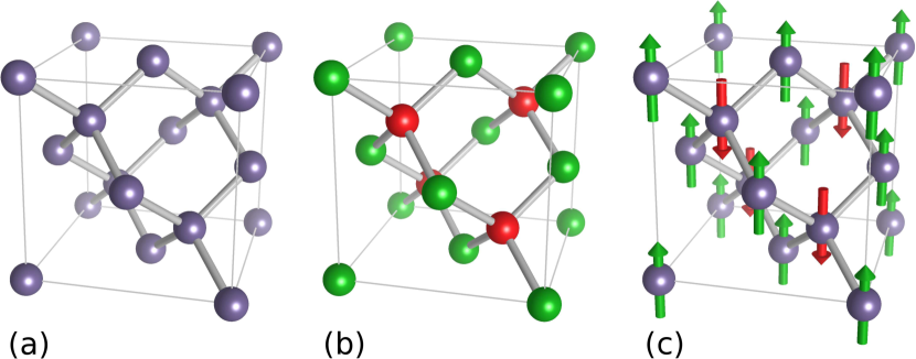
Figure 1: Variations of the diamond structure considered in this work. (a) Inversion-symmetric diamond structure. (b) Zincblende structure that breaks inversion symmetry. (c) Antiferromagnetic diamond structure that breaks time-reversal symmetry $\Theta$ and inversion symmetry $I$ (though the joint operation $\Theta I$ remains a good symmetry). Materials with structure (a) are not magnetoelectric. Those with structure (b) become magnetoelectric when they are magnetized, whereas materials with structure (c) are intrinsically magnetoelectric.

Magnetoelectricity occurs most prominently in antiferromagnetically ordered materials, where an electrically induced magnetization is not masked by an intrinsic magnetization in the system. Similar to ferromagnetic order, antiferromagnetic order can have a spin component and an orbital component, and we can have spontaneous antiferromagnetic order due to a staggered exchange field in the material, but the order can also be induced in both paramagnets and ferromagnets. Here we consider the antiferromagnetic diamond structure shown in Fig. 1(c). To study the magnetoelectricity exhibited in quantum wells made from such a material, we develop a ${\bm{\mathrm{k}}}\cdot{\bm{\mathrm{p}}}$ envelope-function theory for itinerant-electron diamond antiferromagnets, which is in itself an important result presented in this work. On the basis of this theory, we are able to define an operator ${\bm{\mathrm{\tau}}}$ in terms of itinerant-electron degrees of freedom such that a nonzero expectation value $\braket{{\bm{\mathrm{\tau}}}}$ signals collinear antiferromagnetic order in the same way that a nonzero expectation value $\braket{{\bm{\mathrm{\sigma}}}}$ of the charge carriers’ spin operator ${\bm{\mathrm{\sigma}}}$ signals ferromagnetic order of spins. Applying our theoretical framework to antiferromagnetically ordered quantum wells placed into external magnetic and electric fields, we reveal them to exhibit magnetoelectric couplings remarkably similar to those found for the ferromagnetically ordered zincblende quantum wells described above. The magnetoelectric response of the antiferromagnetic system can be related to the modification of the quadrupolar equilibrium-current distribution associated with antiferromagnetic order by external electric and magnetic fields. This is in line with the fact that the magnetoelectric tensor $\alpha_{ij}$ behaves under symmetry transformations like a magnetic quadrupole moment [50], i.e., both of these second-rank material tensors require broken space-inversion symmetry and broken time-reversal symmetry and these tensors share the same pattern of nonzero components, though microscopically they are generally not simply related with each other.

Analytical results obtained from effective two-band models of confined charge carriers elucidate the basic physical phenomena associated with magnetoelectricity in para-, ferro- and antiferromagnetic quantum wells. Accurate numerical calculations utilizing realistic $8\times 8$ and $14\times 14$ ${\bm{\mathrm{k}}}\cdot{\bm{\mathrm{p}}}$ Hamiltonians establish a typically large, practically relevant magnitude of the electric-field-induced magnetization in hole-doped quantum wells made from zincblende ferromagnets or diamond-structure antiferromagnets. The ability to illustrate the full complementarity of magnetoelectric responses within the same microscopic theory distinguishes our approach from most previous ones [14]. We show that our explicit results for the magnetic responses provide an important benchmark for general theories of magnetoelectricity [50, 51, 52]. Our findings provide a platform for further systematic studies aimed at manipulating charges, currents, and magnetic order in solids.

The remainder of this Article is organized as follows. In Sec. II, we define the relevant quantities of interest for our study, establishing the relation between the thermodynamic definitions of polarization (2a) and magnetization (2b) and the electromagnetic definitions of these quantities. We then proceed, in Sec. III, to calculate magnetoelectric responses of quasi-2D electron and hole systems realized in zincblende heterostructures having a Zeeman spin splitting due to an external magnetic field or due to the coupling to ferromagnetic exchange fields. In Sec. IV, we develop a general framework for the ${\bm{\mathrm{k}}}\cdot{\bm{\mathrm{p}}}$ envelope-function description of antiferromagnetic order. We use this framework to perform a comprehensive analysis of magnetoelectric phenomena in quantum wells made from diamond-structure antiferromagnets. Section V is devoted to deriving an upper bound on the magnitude of magnetoelectric-tensor components in quasi-2D systems [53]. We summarize our conclusions and provide a brief outlook in Sec. VI. Appendix A reviews current-induced magnetization, a phenomenon that shares some apparent similarities with the magnetoelectric effect. Ancillary results are presented in Appendices B and C.

II Electric and magnetic responses in quasi-2D systems

We consider a quasi-2D system in the $(x,y)$ plane with open boundary conditions in the $z$ direction in the presence of a perpendicular electric field $\mathcal{E}_{z}$ and an in-plane magnetic field ${\bm{\mathcal{B}}}_{\|}=(\mathcal{B}_{x},\mathcal{B}_{y})$ [44]. Throughout this work, vectors like ${\bm{\mathcal{B}}}_{\|}$ that have only in-plane components will be indicated by a subscript ‘$\|$’, and their vanishing $z$ component will be suppressed. Very generally, the polarization and magnetization can be obtained from the free-energy density $F$ via the relations [11]

$$\mathcal{P}_{z} =-\frac{\partial F}{\partial\mathcal{E}_{z}}\;,$$ (3a)

$${\bm{\mathcal{M}}}_{\|} =-\frac{\partial F}{\partial{\bm{\mathcal{B}}}_{\|}}\;.$$ (3b)

More accurately, the polarization and magnetization only depend on the change of the free energy $\delta F\equiv F(\mathcal{E}_{z},{\bm{\mathcal{B}}}_{\|})-F(0,{\bm{\mathrm{0}}})$ due to the fields $\mathcal{E}_{z}$ and ${\bm{\mathcal{B}}}_{\|}$.

To simplify the analysis, we assume that only the itinerant charge carriers in the quasi-2D system contribute to the electric and magnetic response. We assume that the confining potential $V(z)$ of the quasi-2D system includes the electrostatic potential due to compensating charges and external gates that ensure overall charge neutrality and that are assumed to be fixed in space. Also, we assume that the potential $V(z)$ defining a quantum well for the quasi-2D system is symmetric, i.e., $V(-z)=V(z)$. We denote the Hamiltonian for the charge carriers by $H$. The electric field $\mathcal{E}_{z}$ enters $H$ via the additional potential $e\mathcal{E}_{z}z$, where $e\equiv|e|$ is the elementary charge. The magnetic field ${\bm{\mathcal{B}}}_{\|}$ enters $H$ via the vector potential ${\bm{\mathcal{A}}}$ that is related to the magnetic field via ${\bm{\mathcal{B}}}_{\|}={\bm{\mathrm{\nabla}}}\times{\bm{\mathcal{A}}}$, with ${\bm{\mathrm{\nabla}}}$ denoting the gradient w.r.t. the position vector ${\bm{\mathrm{r}}}\equiv(x,y,z)$. In addition, ${\bm{\mathcal{B}}}_{\|}$ may enter $H$ via a Zeeman term $(g/2)\mu_{\mathrm{B}}\,{\bm{\mathrm{\sigma}}}\cdot{\bm{\mathcal{B}}}_{\|}$, where $g$ denotes the $g$ factor, $\mu_{\mathrm{B}}\equiv e\hbar/(2m_{0})$ is the Bohr magneton, with $m_{0}$ being the mass of free electrons, and ${\bm{\mathrm{\sigma}}}$ is a dimensionless spin operator . The eigenstates of $H$ associated with eigenvalues $E_{n{\bm{\mathrm{k}}}_{\|}}$ have the general form

$$\Psi_{n{\bm{\mathrm{k}}}_{\|}}({\bm{\mathrm{r}}})=\frac{\mathrm{e}^{i{\bm{\mathrm{k}}}_{\|}\cdot{\bm{\mathrm{r}}}}}{2\pi}\,\Phi_{n{\bm{\mathrm{k}}}_{\|}}(z)\;.$$ (4)

Here $n$ labels the quasi-2D subbands, and ${\bm{\mathrm{k}}}_{\|}\equiv(k_{x},k_{y})$ is the in-plane wave vector. The free-energy density can then be written in the form

$$F=\frac{1}{w}\sum_{n}\int\frac{d^{2}k_{\|}}{(2\pi)^{2}}\;f(E_{n{\bm{\mathrm{k}}}_{\|}})\;E_{n{\bm{\mathrm{k}}}_{\|}}\quad,$$ (5)

where $w$ is the width of the quantum well, and $f(E)$ denotes the Fermi distribution function. We will later assume zero temperature so that $f(E)$ becomes a step function $f(E)=\Theta(E_{\mathrm{F}}-E)$, with the Fermi energy $E_{\mathrm{F}}$.

Using the expression (5) for the free-energy density, the polarization becomes

$$\mathcal{P}_{z}=\mathcal{P}_{z}^{\mathrm{e}}+\mathcal{P}_{z}^{\mathrm{q}}\,\,,$$ (6)

with

$$\mathcal{P}_{z}^{\mathrm{e}} =-\frac{1}{w}\sum_{n}\int\frac{d^{2}k_{\|}}{(2\pi)^{2}}\;f(E_{n{\bm{\mathrm{k}}}_{\|}})\,\frac{\partial E_{n{\bm{\mathrm{k}}}_{\|}}}{\partial\mathcal{E}_{z}}\;,$$ (7a)

$$\mathcal{P}_{z}^{\mathrm{q}} =-\frac{1}{w}\sum_{n}\int\frac{d^{2}k_{\|}}{(2\pi)^{2}}\;E_{n{\bm{\mathrm{k}}}_{\|}}\,\frac{\partial f(E_{n{\bm{\mathrm{k}}}_{\|}})}{\partial\mathcal{E}_{z}}\;.$$ (7b)

The first term $\mathcal{P}_{z}^{\mathrm{e}}$ arises from the $\mathcal{E}_{z}$-dependence of the energies $E_{n{\bm{\mathrm{k}}}_{\|}}$ of occupied states. The second term $\mathcal{P}_{z}^{\mathrm{q}}$ represents a quantum-kinetic [55] contribution to $\mathcal{P}_{z}$ that accounts for changes in the equilibrium occupation-number distribution arising from a change of $\mathcal{E}_{z}$. Hence, in the low-temperature limit, $\mathcal{P}_{z}^{\mathrm{q}}$ reflects $\mathcal{E}_{z}$-induced changes in the shape or topology of the Fermi surface.

Using the Hellmann-Feynman theorem and assuming the only explicit $\mathcal{E}_{z}$-dependence in the Hamiltonian $H$ to be the potential $e\mathcal{E}_{z}z$ , we find

$$\mathcal{P}_{z}^{\mathrm{e}}=-\frac{e}{w}\sum_{n}\int\frac{d^{2}k_{\|}}{(2\pi)^{2}}\;f(E_{n{\bm{\mathrm{k}}}_{\|}})\,\braket{z}_{n{\bm{\mathrm{k}}}_{\|}}\;,$$ (8)

where

$$\braket{z}_{n{\bm{\mathrm{k}}}_{\|}}=\int dz\,\left|\Phi_{n{\bm{\mathrm{k}}}_{\|}}(z)\right|^{2}\,z$$ (9)

denotes the displacement of an electron in the state $\Phi_{n{\bm{\mathrm{k}}}_{\|}}(z)$. Thus the term $\mathcal{P}_{z}^{\mathrm{e}}$ coincides with the electrostatic definition of polarization as the volume average of microscopic electric dipole moments [57, 58]. In a quasi-2D system with open boundary conditions in the $z$ direction (and overall charge neutrality as assumed above), the electrostatic polarization $\mathcal{P}_{z}^{\mathrm{e}}$ is unambiguously defined independently of the origin of the coordinate system. It avoids the technical problems inherent in studies of the bulk (3D) polarization [58]. The average displacement of the occupied states is

$$\braket{z} =\frac{1}{N_{\mathrm{s}}}\sum_{n}\int\frac{d^{2}k_{\|}}{(2\pi)^{2}}\,f(E_{n{\bm{\mathrm{k}}}_{\|}})\,\braket{z}_{n{\bm{\mathrm{k}}}_{\|}}\;,$$ (10a)

$$=\frac{1}{N_{\mathrm{s}}}\int dz\>\rho(z)\,z\;,$$ (10b)

where

$$\rho(z)=\sum_{n}\int\frac{d^{2}k_{\|}}{(2\pi)^{2}}\,\,f(E_{n{\bm{\mathrm{k}}}_{\|}})\,\,\left|\Phi_{n{\bm{\mathrm{k}}}_{\|}}(z)\right|^{2}$$ (11)

is the 3D number density, and $N_{\mathrm{s}}=\int dz\,\rho(z)$ is the 2D (sheet) density of charge carriers in the quantum well. Thus we can rewrite the polarization (8) as

$$\mathcal{P}_{z}^{\mathrm{e}}=\mathcal{P}_{0}\,P\equiv\mathcal{P}_{0}\frac{\braket{z}}{w}\quad,$$ (12)

where $\mathcal{P}_{0}\equiv-eN_{\mathrm{s}}$, and the dimensionless number $P=\braket{z}/w$ describes the average polarization per particle.

Similar to the polarization $\mathcal{P}_{z}$, the magnetization ${\bm{\mathcal{M}}}_{\|}$ is also the sum of two contributions,

$${\bm{\mathcal{M}}}_{\|}={\bm{\mathcal{M}}}_{\|}^{\mathrm{e}}+{\bm{\mathcal{M}}}_{\|}^{\mathrm{q}}\,\,,$$ (13)

with

$${\bm{\mathcal{M}}}_{\|}^{\mathrm{e}} =-\frac{1}{w}\sum_{n}\int\frac{d^{2}k_{\|}}{(2\pi)^{2}}\;f(E_{n{\bm{\mathrm{k}}}_{\|}})\,\frac{\partial E_{n{\bm{\mathrm{k}}}_{\|}}}{\partial{\bm{\mathcal{B}}}_{\|}}\;,$$ (14a)

$${\bm{\mathcal{M}}}_{\|}^{\mathrm{q}} =-\frac{1}{w}\sum_{n}\int\frac{d^{2}k_{\|}}{(2\pi)^{2}}\;E_{n{\bm{\mathrm{k}}}_{\|}}\,\frac{\partial f(E_{n{\bm{\mathrm{k}}}_{\|}})}{\partial{\bm{\mathcal{B}}}_{\|}}\;,$$ (14b)

which again represent the electromagnetic and the quantum-kinetic effects of ${\bm{\mathcal{B}}}_{\|}$, respectively. Given that ${\bm{\mathcal{B}}}_{\|}$ generally enters the Hamiltonian $H$ via both the vector potential ${\bm{\mathcal{A}}}$ and also via the Zeeman term, the contribution ${\bm{\mathcal{M}}}_{\|}^{\mathrm{e}}$ can be split further into orbital and spin contributions,

$${\bm{\mathcal{M}}}_{\|}^{\mathrm{e}}={\bm{\mathcal{M}}}_{\|}^{\mathrm{o}}+{\bm{\mathcal{S}}}_{\|}\;,$$ (15)

where

$${\bm{\mathcal{M}}}_{\|}^{\mathrm{o}} =-\frac{1}{w}\sum_{n}\int\frac{d^{2}k_{\|}}{(2\pi)^{2}}\;f(E_{n{\bm{\mathrm{k}}}_{\|}})\,\Big{\langle}\sum_{j=x,y}\frac{\partial H}{\partial\mathcal{A}_{j}}\frac{\partial\mathcal{A}_{j}}{\partial{\bm{\mathcal{B}}}_{\|}}\Big{\rangle}_{n{\bm{\mathrm{k}}}_{\|}}\,,$$

$$=-\frac{e}{w}\sum_{n}\int\frac{d^{2}k_{\|}}{(2\pi)^{2}}\,\,f(E_{n{\bm{\mathrm{k}}}_{\|}})\,\,\hat{{\bm{\mathrm{z}}}}\times\braket{\{z\,,{\bm{\mathrm{v}}}}{\}}_{n{\bm{\mathrm{k}}}_{\|}}\,\,,$$ (16a)

$${\bm{\mathcal{S}}}_{\|} =-\frac{1}{w}\sum_{n}\int\frac{d^{2}k_{\|}}{(2\pi)^{2}}\;f(E_{n{\bm{\mathrm{k}}}_{\|}})\,\Big{\langle}\frac{\partial H}{\partial{\bm{\mathcal{B}}}_{\|}}\Big{\rangle}_{n{\bm{\mathrm{k}}}_{\|}}\;,$$

$$=-\frac{g\mu_{\mathrm{B}}}{2w}\sum_{n}\int\frac{d^{2}k_{\|}}{(2\pi)^{2}}\,f(E_{n{\bm{\mathrm{k}}}_{\|}})\,\braket{{\bm{\mathrm{\sigma}}}}_{n{\bm{\mathrm{k}}}_{\|}}\;.$$ (16b)

To obtain Eqs. (16a) and (16b), we used once again the Hellmann-Feynman theorem. The first term ${\bm{\mathcal{M}}}_{\|}^{\mathrm{o}}$ represents the in-plane orbital magnetization [57, 58]. In Eq. (16a), the symbol ${\bm{\mathrm{v}}}_{\|}\equiv\partial H/(\partial\hbar{\bm{\mathrm{k}}}_{\|})$ denotes the in-plane component of the velocity operator, and

$$\braket{\{z\,,{\bm{\mathrm{v}}}}{\}}_{n{\bm{\mathrm{k}}}_{\|}}=\int dz\;\;\Phi^{\dagger}_{n{\bm{\mathrm{k}}}_{\|}}(z)\,\,\{z\,,{\bm{\mathrm{v}}}_{\|}\}\,\,\Phi_{n{\bm{\mathrm{k}}}_{\|}}(z)\,\,,$$ (17)

with $\{A,B\}\equiv\frac{1}{2}(AB+BA)$. The expression (16a) is associated with the vector potential ${\bm{\mathcal{A}}}=z\,{\bm{\mathcal{B}}}_{\|}\times\hat{{\bm{\mathrm{z}}}}$ that is adopted throughout our work as the appropriate gauge for quasi-2D systems. This is the reason why Eq. (16a) differs from the conventional formula for the orbital magnetization [58] that is obtained for the symmetric gauge [59] ${\bm{\mathcal{A}}}^{\mathrm{sym}}\equiv\frac{1}{2}\,{\bm{\mathcal{B}}}\times{\bm{\mathrm{r}}}$, see Appendix B. Similar to $\mathcal{P}_{z}^{\mathrm{e}}$, the magnetization ${\bm{\mathcal{M}}}_{\|}^{\mathrm{o}}$ of a quasi-2D system avoids the technical problems inherent in studies of the bulk (3D) orbital magnetization [58]; it is unambiguously defined independently of the origin of the coordinate system.

An orbital magnetization ${\bm{\mathcal{M}}}_{\|}^{\mathrm{o}}$ is generally accompanied by a nonvanishing in-plane current distribution

$${\bm{\mathcal{j}}}_{\|}(z)=-e\sum_{n}\!\int\!\frac{d^{2}k_{\|}}{(2\pi)^{2}}\,f(E_{n{\bm{\mathrm{k}}}_{\|}})\,{\bm{\mathrm{j}}}_{\|}(z,n{\bm{\mathrm{k}}}_{\|})\,\,,$$ (18a)

with

$${\bm{\mathrm{j}}}_{\|}(z,n{\bm{\mathrm{k}}}_{\|})=\Re\mathrm{e}\,\!\Big{[}\Phi_{n{\bm{\mathrm{k}}}_{\|}}^{\dagger}(z)\,{\bm{\mathrm{v}}}_{\|}\,\Phi_{n{\bm{\mathrm{k}}}_{\|}}(z)\Bigr{]}\,\,,$$ (18b)

though in thermal equilibrium, the total current ${\bm{\mathcal{J}}}_{\|}=\int dz\,{\bm{\mathcal{j}}}_{\|}(z)$ is always zero. These currents ${\bm{\mathcal{j}}}_{\|}(z)$ are nondissipative because they are not driven by an electric field. (Throughout this work, we assume ${\bm{\mathcal{E}}}_{\|}={\bm{\mathrm{0}}}$ for the in-plane electric field.) Direct experimental observation of the currents ${\bm{\mathcal{j}}}_{\|}(z)$ seems impossible, as their nature appears to preclude any ability to make contact to them. However, their ramification in terms of the magnetization ${\bm{\mathcal{M}}}_{\|}^{\mathrm{o}}$ is detectable.

The second term ${\bm{\mathcal{S}}}_{\|}$ in Eq. (15) represents the spin magnetization, given in Eq. (16b) in terms of the dimensionless spin polarization $\braket{{\bm{\mathrm{\sigma}}}}_{n{\bm{\mathrm{k}}}_{\|}}$ of individual states. We rewrite this as

$${\bm{\mathcal{S}}}_{\|}=-\frac{g\mu_{\mathrm{B}}N_{\mathrm{s}}}{2w}\,{\bm{\mathrm{S}}}_{\|}\;,$$ (19)

where ${\bm{\mathrm{S}}}_{\|}$ is the dimensionless average spin polarization of the entire system. Similarly, it is convenient to define ${\bm{\mathcal{M}}}_{\|}^{\mathrm{o}}=\mathcal{M}_{0}\,{\bm{\mathrm{M}}}_{\|}^{\mathrm{o}}$ with $\mathcal{M}_{0}\equiv-\mu_{\mathrm{B}}N_{\mathrm{s}}/w$ and dimensionless ${\bm{\mathrm{M}}}_{\|}^{\mathrm{o}}$ so that we get

$${\bm{\mathcal{M}}}_{\|}^{\mathrm{e}} =\mathcal{M}_{0}\left({\bm{\mathrm{M}}}_{\|}^{\mathrm{o}}+\frac{g}{2}\,{\bm{\mathrm{S}}}_{\|}\right)\,\,,$$ (20a)

$$=\frac{\mathcal{M}_{0}}{N_{\mathrm{s}}}\int\frac{d^{2}k_{\|}}{(2\pi)^{2}}\,f(E_{n{\bm{\mathrm{k}}}_{\|}})$$

$$\hskip 15.00002pt{}\times\left[\frac{2m_{0}}{\hbar}\,\hat{{\bm{\mathrm{z}}}}\times\braket{\{z\,,{\bm{\mathrm{v}}}}{\}}_{n{\bm{\mathrm{k}}}_{\|}}+\frac{g}{2}\,\braket{{\bm{\mathrm{\sigma}}}}_{n{\bm{\mathrm{k}}}_{\|}}\right]\,\,.$$ (20b)

A polarization $\mathcal{P}_{z}^{\mathrm{e}}$ represents the dipole term ($l=1$) in a multipole expansion of a charge distribution $\rho(z)$ [57]. Similarly, an orbital magnetization ${\bm{\mathcal{M}}}_{\|}^{\mathrm{o}}$ represents the dipole term ($l=1$) in a multipole expansion of a current distribution ${\bm{\mathcal{j}}}_{\|}(z)$. Charge neutrality of a localized charge distribution $\rho(z)$ generally requires a vanishing monopole ($l=0$) for the multipole expansion of $\rho(z)$. Similarly, a localized current distribution ${\bm{\mathcal{j}}}_{\|}(z)$ requires a vanishing monopole for the multipole expansion of ${\bm{\mathcal{j}}}_{\|}(z)$. An equilibrium current distribution ${\bm{\mathcal{j}}}_{\|}(z)$ that breaks time-reversal symmetry is permitted in ferromagnets and in antiferromagnets [60]. The finite magnetization in ferromagnets implies that the equilibrium current distribution ${\bm{\mathcal{j}}}_{\|}(z)$ includes a dipolar component ($l=1$), whereas the vanishing magnetization in antiferromagnets requires equilibrium currents to be (at least) of quadrupolar type ($l=2$).

For finite systems, the lowest nonvanishing multipole in a multipole expansion is generally independent of the origin of the coordinate system and in that sense well-defined, whereas higher multipoles depend on the choice for the origin [57]. We therefore limit our discussion below to the lowest nonvanishing multipole. As mentioned above, in infinite periodic crystals, even the lowest nonvanishing multipole moment requires a more careful treatment [58].

As integrals can be more easily and more reliably calculated numerically than derivatives [61], it is more straightforward to evaluate numerically the integrals defining the electromagnetic parts $\mathcal{P}_{z}^{\mathrm{e}}$, ${\bm{\mathcal{M}}}_{\|}^{\mathrm{o}}$, and ${\bm{\mathcal{S}}}_{\|}$ of the response functions. On the other hand, it is more difficult to evaluate accurately the full response functions $P_{z}$ and ${\bm{\mathcal{M}}}_{\|}$ that require a numerical differentiation of the free energy $F$ as a function of the applied external fields [62, 63]. A detailed account of these technical issues is beyond the scope of the present work. In the following, we thus focus on $P_{z}^{\mathrm{e}}$, ${\bm{\mathcal{M}}}_{\|}^{\mathrm{o}}$, and ${\bm{\mathcal{S}}}_{\|}$ alone. This is adequate for scenarios where the quantum-kinetic parts $P_{z}^{\mathrm{q}}$ and ${\bm{\mathcal{M}}}_{\|}^{\mathrm{q}}$ of the response functions are less important, which we have found to be generally the case for a strong confinement $V(z)$. Within the framework of the analytical perturbative calculations of the magnetoelectric effect discussed below, the external fields $\mathcal{E}_{z}$ and ${\bm{\mathcal{B}}}_{\|}$ do not change the occupation of individual states. Quantum-kinetic contributions $\mathcal{P}_{z}^{\mathrm{q}}$ and ${\bm{\mathcal{M}}}_{\|}^{\mathrm{q}}$ thus do not arise in the analytical calculations.

III Magnetoelectricity in zincblende paramagnets and ferromagnets

III.1 The model

The diamond crystal structure is shown in Fig. 1(a). Space inversion is a good symmetry in diamond so that electronic states are at least twofold degenerate throughout the Brillouin zone [45]. The diamond structure is realized in group-IV semiconductors including C, Si, and Ge. In a zincblende structure, the atomic sites in a diamond structure are alternatingly occupied by two different atoms such as Ga and As or In and Sb [Fig. 1(b)]. Thus spin degeneracy of the electronic states is lifted in paramagnetic zincblende structures except for ${\bm{\mathrm{k}}}={\bm{\mathrm{0}}}$.

Spontaneous ferromagnetic order is realized in semiconductors with zincblende structure such as GaMnAs [64] and InMnSb [65], where the ferromagnetic coupling between local Mn moments is mediated by itinerant holes [46, 47]. In ferromagnetic GaMnAs, the magnetization resides mostly in the Mn-impurity spins (with magnetic moment $5\,\mu_{\mathrm{B}}$) [47, 46]. We want to focus here on ferromagnetic InSb, where the effective spin magnetic moment of holes $\sim 2\kappa\mu_{\mathrm{B}}$ (with Luttinger parameter $\kappa=15.6$) is more than an order of magnitude larger than in GaAs ($\kappa=1.2$), so that the magnetization density residing in spin-polarized itinerant InSb holes can easily exceed the magnetization density due to Mn spins (assuming hole densities comparable to the densities of Mn acceptors, although the hole densities can also be controlled independently by means of external gates). In the present work, we thus focus on the itinerant carriers, assuming for conceptual clarity that the spontaneous magnetization ${\bm{\mathcal{M}}}^{\mathrm{s}}$ is fixed [49]. The more complicated band structure of holes can only be satisfactorily approached in less transparent numerical calculations. Therefore, we complement the calculations for holes with more transparent calculations for electron systems.

For common semiconductors with a zincblende structure, such as GaAs, InAs, and InSb, the electronic states in a quantum well can be described by a multiband Hamiltonian [66]

$$\mathcal{H}=\mathcal{H}_{k}+V(z)+\mathcal{H}_{\mathrm{D}}+\mathcal{H}_{\mathcal{Z}}+e\mathcal{E}_{z}z\quad.$$ (21)

Here $\mathcal{H}_{k}$ is the inversion-symmetric part of $\mathcal{H}$, and $\mathcal{H}_{\mathrm{D}}$ subsumes Dresselhaus terms due to bulk inversion asymmetry (BIA). $V(z)$ is the quantum-well confinement, so that the wave vector ${\bm{\mathrm{k}}}_{\|}=(k_{x},k_{y})$ is a good quantum number, whereas $k_{z}$ becomes the operator $-i\partial_{z}$. An external electric field $\mathcal{E}_{z}$ can be included in $\mathcal{H}$ by adding the potential $e\mathcal{E}_{z}z$. Similarly, an external in-plane magnetic field ${\bm{\mathcal{B}}}_{\|}$ can be included in $\mathcal{H}$ via the vector potential ${\bm{\mathcal{A}}}=z\,{\bm{\mathcal{B}}}_{\|}\times\hat{{\bm{\mathrm{z}}}}$. In $\mathcal{H}_{k}+\mathcal{H}_{D}$ we then replace ${\bm{\mathrm{k}}}$ by the kinetic wave vector ${\bm{\mathcal{k}}}={\bm{\mathrm{k}}}+\frac{e}{\hbar}{\bm{\mathcal{A}}}$. The Zeeman term $\mathcal{H}_{\mathcal{Z}}$ includes contributions from both the external field ${\bm{\mathcal{B}}}_{\|}$ and possibly a ferromagnetic exchange interaction represented by an internal exchange field ${\bm{\mathcal{X}}}_{\|}$ that is likewise assumed to be in-plane. A finite exchange field ${\bm{\mathcal{X}}}_{\|}$ corresponds to a finite spontaneous magnetization ${\bm{\mathcal{M}}}^{\mathrm{s}}$ in the expansion (I). For $\mathcal{X}=0$, the system is a paramagnet, where the lowest-order term in the expansion (I) that depends only on ${\bm{\mathcal{B}}}$ is $-{\textstyle\frac{1}{2}}\mu_{0}^{-1}\,\chi^{\mathcal{B}}_{ij}\,\mathcal{B}_{i}\mathcal{B}_{j}$, signifying the fact that the system’s magnetization scales with the applied field ${\bm{\mathcal{B}}}$ until the system is fully spin-polarized. For the magnetoelectric effect studied here, a finite Zeeman term $\mathcal{H}_{\mathcal{Z}}$ indicates, first of all, a breaking of time-reversal symmetry so that the origin of $\mathcal{H}_{\mathcal{Z}}$ is largely irrelevant for the microscopic mechanism yielding the magnetoelectric response. Nonetheless, as to be expected, we will see below that only for $\mathcal{X}\neq 0$ or a fully spin-polarized paramagnet, the final result for the lowest-order magnetoelectric contribution to the free energy (I) can be expressed via a tensor $\alpha_{ij}$, whereas in partially spin-polarized paramagnets the linear dependence of $\mathcal{H}_{\mathcal{Z}}$ on ${\bm{\mathcal{B}}}_{\|}$ is the reason why in lowest order we get terms in Eq. (I) that are weighted by a third-rank tensor $\beta_{ijk}$.

The diagonalization of the Hamiltonian (21) yields the eigenenergies $E_{n{\bm{\mathrm{k}}}_{\|}}$ with associated bound states $\Phi_{n{\bm{\mathrm{k}}}_{\|}}(z)\equiv\braket{z}{n{\bm{\mathrm{k}}}}{}$, where $n$ is the subband index. In the numerical calculations presented below, we use for $\mathcal{H}$ the $8\times 8$ Kane model and the $14\times 14$ extended Kane model as defined in Table C.5 of Ref. [66]. Confinement in the quasi-2D system is due to a finite potential well $V(z)=V_{0}\,\Theta(|z|-w/2)$ with barrier height $V_{0}$. The numerical solution of $\mathcal{H}$ is based on a quadrature method [67]. We evaluate $k$-space integrals such as Eq. (8) by means of analytic quadratic Brillouin-zone integration [68].

Before presenting numerical results for multi-band models, we illustrate the physical origin and ramifications of magnetoelectricity in zincblende-semiconductor quantum wells by analytical calculations. Specifically, we consider a $2\times 2$ model for the $\Gamma_{6}$ conduction band

$$\mathsf{H}=\mathsf{H}_{k}+V(z)+\mathsf{H}_{\mathrm{D}}+\mathsf{H}_{\mathcal{Z}}+e\mathcal{E}_{z}z\,\,,$$ (22a)

with

$$\mathsf{H}_{k} =\frac{\hbar^{2}\mathcal{k}^{2}}{2m}\,\,,$$ (22b)

$$\rule{0.0pt}{17.22217pt}\mathsf{H}_{\mathrm{D}} =d\left(\left\{\mathcal{k}_{x},\mathcal{k}_{y}^{2}-\mathcal{k}_{z}^{2}\right\}\sigma_{x}+\mbox{cp}\right)\,\,,$$ (22c)

$$\mathsf{H}_{\mathcal{Z}} ={\bm{\mathcal{Z}}}\cdot{\bm{\mathrm{\sigma}}}\,\,,$$ (22d)

where $m$ denotes the effective mass, $\mathsf{H}_{\mathrm{D}}$ is the Dresselhaus term with prefactor $d$, cp denotes cyclic permutation of the preceding term, ${\bm{\mathrm{\sigma}}}\equiv(\sigma_{x},\sigma_{y},\sigma_{z})$ is the vector of Pauli matrices, and $\mathsf{H}_{\mathcal{Z}}$ is the Zeeman term that depends on the total field ${\bm{\mathcal{Z}}}\equiv(g/2)\,\mu_{\mathrm{B}}\,{\bm{\mathcal{B}}}_{\|}+{\bm{\mathcal{X}}}_{\|}$. Considering the transparent $2\times 2$ model $\mathsf{H}$ turns out to be useful because it captures the important physical trends, even though it does not include certain details [such as nonparabolicity and corrections to the Dresselhaus spin splitting (22c)] that are included in $\mathcal{H}$ and that would be required for a quantitatively reliable account of specific experiments. The relation between the simplified Hamiltonian $\mathsf{H}$ and the more complete Hamiltonian $\mathcal{H}$ is discussed in more detail, e.g., in Ref. [66].

From now on, the direction of ${\bm{\mathcal{Z}}}$ is chosen as the spin-quantization axis for convenience. We will be interested in terms at most quadratic in ${\bm{\mathcal{k}}}_{\|}$ and linear in $\mathcal{B}_{\|}$, where the latter is justified for weak fields $\mathcal{B}_{\|}$, i.e., when the well width $w$ is smaller than the magnetic length $\sqrt{\hbar/|e\mathcal{B}_{\|}|}$. Then the Hamiltonian $\mathsf{H}$ becomes [69]

$$\mathsf{H} =\frac{\hbar^{2}\mathcal{k}^{2}}{2m}+V(z)+d\,k_{z}^{2}\left[\left(\mathcal{k}_{x}\sin\varphi_{\mathcal{Z}}+\mathcal{k}_{y}\cos\varphi_{\mathcal{Z}}\right)\sigma_{x}-\left(\mathcal{k}_{x}\cos\varphi_{\mathcal{Z}}-\mathcal{k}_{y}\sin\varphi_{\mathcal{Z}}\right)\sigma_{z}\right]+\mathcal{Z}\,\sigma_{z}+e\mathcal{E}_{z}z\,\,,$$ (23a)

$$=\frac{\hbar^{2}\mathcal{k}_{z}^{2}}{2m}+V(z)+\frac{\hbar^{2}}{2m}\left({\bm{\mathcal{k}}}_{\|}-{\bm{\mathrm{k}}}_{0}\right)^{2}-\frac{\hbar^{2}k_{0}^{2}}{2m}+\mathcal{Z}\,\sigma_{z}+e\mathcal{E}_{z}z\,\,,$$ (23b)

with

$${\bm{\mathrm{k}}}_{0}=\frac{m}{\hbar^{2}}\,d\,k_{z}^{2}\left[\begin{pmatrix}\cos\varphi_{\mathcal{Z}}\\ -\sin\varphi_{\mathcal{Z}}\end{pmatrix}\sigma_{z}-\begin{pmatrix}\sin\varphi_{\mathcal{Z}}\\ \cos\varphi_{\mathcal{Z}}\end{pmatrix}\sigma_{x}\right]\,\,,$$ (24)

and $\varphi_{\mathcal{Z}}$ is the angle between the total Zeeman field ${\bm{\mathcal{Z}}}$ and the crystallographic direction $[100]$. The usefulness of writing $\mathsf{H}$ as in Eq. (23b) will become clear later on.

For $\mathcal{E}_{z}=0$ and $\mathcal{B}_{\|}=0$, the Hamiltonian is

$$\mathsf{H}=\mathsf{H}^{(0)}+\mathsf{H}_{\mathcal{Z}}^{(0)}+\mathsf{H}_{\mathrm{D}}^{(1)}\,\,,$$ (25)

with

$$\mathsf{H}^{(0)} = \frac{\hbar^{2}k_{z}^{2}}{2m}+V(z)\,\,,$$ (26a)

$$\mathsf{H}_{\mathcal{Z}}^{(0)} = \mathcal{Z}\,\sigma_{z}\,\,,$$ (26b)

$$\mathsf{H}_{\mathrm{D}}^{(1)} = \frac{\hbar^{2}}{2m}\left({\bm{\mathrm{k}}}_{\|}-{\bm{\mathrm{k}}}_{0}\right)^{2}-\frac{\hbar^{2}k_{0}^{2}}{2m}\,\,.$$ (26c)

The eigenstates of $\mathsf{H}^{(0)}+\mathsf{H}_{\mathcal{Z}}^{(0)}$ are $\ket{\nu\sigma^{(0)}}\equiv\ket{\nu}\otimes\ket{\sigma}$, with associated eigenvalues $E_{\nu\sigma,{\bm{\mathrm{0}}}}\equiv E_{\nu}^{(0)}+\sigma\,\mathcal{Z}$, where $\sigma=\pm 1$. Treating $\mathsf{H}_{\mathrm{D}}^{(1)}$ in first order, the subband dispersions are

$$E_{\nu\sigma,{\bm{\mathrm{k}}}_{\|}}=E_{\nu}^{(0)}+\frac{\hbar^{2}k_{\|}^{2}}{2m}+\sigma\sqrt{d\,\braket{k_{z}^{2}}\,k_{\|}^{2}+\mathcal{Z}\left[\mathcal{Z}-2d\,\braket{k_{z}^{2}}\,(k_{x}\cos\varphi_{\mathcal{Z}}-k_{y}\sin\varphi_{\mathcal{Z}})\right]}\quad,$$ (27)

with $\braket{k_{z}^{2}}=\braket{\nu}{k_{z}^{2}}{\nu}$. For $\mathcal{Z}=0$, the spectrum $E_{\nu\sigma,{\bm{\mathrm{k}}}_{\|}}$ satisfies time-reversal symmetry, $E_{\nu\sigma,-{\bm{\mathrm{k}}}_{\|}}=E_{\nu\sigma,{\bm{\mathrm{k}}}_{\|}}$. For $\mathcal{Z}\neq 0$, the relation $E_{\nu\sigma,-{\bm{\mathrm{k}}}_{\|}}\neq E_{\nu\sigma,{\bm{\mathrm{k}}}_{\|}}$ reflects broken time-reversal symmetry. The latter is a prerequisite for the magnetoelectric effect, as discussed above.

Figures 2(a) and 2(c) illustrate the dispersion (27) for a quasi-2D electron system in a ferromagnetic InSb quantum well with $\mathcal{X}_{x}=8\,$meV, width $w=150\,$Å, and with an electron density $N_{s}=1.0\times 10^{11}\,$cm^-2. The numerical calculations in Fig. 2 are based on the more accurate multiband Hamiltonian $\mathcal{H}$ introduced above. Band parameters for InSb are taken from Ref. [66].

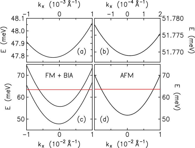
Figure 2: Dispersion of the lowest electron subbands in a quantum well with width $w=150\,$Å and barrier height $V_{0}=1.2\,$eV for $\mathcal{E}_{z}=\mathcal{B}_{\|}=0$. The red lines indicate the Fermi energy for an electron density $N_{s}=1.0\times 10^{11}\,$cm^-2. Left column [panels (a), (c)]: Dispersion $E_{0\pm,k_{x}}$ for ferromagnetic InSb with $\mathcal{X}_{x}=8\,$meV and BIA. Right column [panels (b), (d)]: Dispersion $E_{0k_{x}}$ for a diamond antiferromagnet with InSb band-structure parameters (without BIA) and $\mathcal{Y}_{x}=50\,$meV. The upper panels (a), (b) show a zoom-in of the same dispersion as in panels (c), (d) near $k_{\|}=0$.

III.2 $\mathcal{E}$-induced magnetization

In this section, we evaluate the equilibrium magnetization induced by an electric field $\mathcal{E}_{z}$ using perturbation theory, which is justified by the fact that the $\mathcal{E}$-induced magnetization is commonly a small fraction of the spontaneous magnetization $\mathcal{M}^{\mathrm{s}}_{\|}$ in the system. (See Table 3 below for typical numbers.) We start from the Hamiltonian (23). Specializing to $\mathcal{B}_{\|}=0$ yields

$$\mathsf{H}_{{\bm{\mathcal{M}}}\leftarrow{\bm{\mathcal{E}}}}=\mathsf{H}^{(0)}+\mathsf{H}_{\mathcal{Z}}^{(0)}+\mathsf{H}_{\mathrm{D}}^{(1)}+\mathsf{H}_{\mathcal{E}}^{(1)}\,\,,$$ (28)

with $\mathsf{H}^{(0)}$, $\mathsf{H}_{\mathcal{Z}}^{(0)}$, and $\mathsf{H}_{\mathrm{D}}^{(1)}$ given by Eqs. (26a), (26b), and (26c), respectively, and

$$\mathsf{H}_{\mathcal{E}}^{(1)}=e\mathcal{E}_{z}\,z\,\,.$$ (29)

Treating the electric field $\mathcal{E}_{z}$ in first-order perturbation theory, the eigenstates become

$$\ket{\nu\sigma^{(1)}}=\Bigl{(}\ket{\nu}+e\mathcal{E}_{z}\,\sum_{\nu^{\prime}\neq\nu}c_{\nu^{\prime}\nu}\ket{\nu^{\prime}}\Bigr{)}\otimes\ket{\sigma}\;,$$ (30)

with expansion coefficients

$$c_{\nu^{\prime}\nu}=\frac{\braket{\nu^{\prime}}{z}{\nu}}{E_{\nu}^{(0)}-E_{\nu^{\prime}}^{(0)}}\;.$$ (31)

It will be seen below that, for the calculation of the electric-field-induced magnetization, we can ignore the modification of the states $\ket{\nu\sigma^{(1)}}$ due to $\mathsf{H}_{\mathrm{D}}^{(1)}$ that yields an effect of higher order in the Dresselhaus coefficient $d$. In the following, $\braket{\dots}$ denotes the average in the unperturbed state $\ket{\nu}$, whereas $\lAngle\,\dots\,\rAngle$ denotes the average in the perturbed state $\ket{\nu\sigma^{(1)}}$ in the presence of the external field inducing the magnetoelectric response.

For the equilibrium magnetization (16a), we need to evaluate expectation values $\lAngle\,\{z\,,{\bm{\mathrm{v}}}_{\|}({\bm{\mathrm{k}}}_{\|})\}\,\rAngle$ using the velocity operator associated with the Hamiltonian (28)

$${\bm{\mathrm{v}}}_{\|}({\bm{\mathrm{k}}}_{\|})=\frac{\partial\mathsf{H}_{{\bm{\mathcal{M}}}\leftarrow{\bm{\mathcal{E}}}}}{\partial\,\hbar{\bm{\mathrm{k}}}_{\|}}=\frac{\hbar}{m}\left({\bm{\mathrm{k}}}_{\|}-{\bm{\mathrm{k}}}_{0}\right)\,\,.$$ (32)

We get

$$\lAngle\,\{z\,,{\bm{\mathrm{v}}}_{\|}({\bm{\mathrm{k}}}_{\|})\}\,\rAngle =\lAngle\,z\,\rAngle\lAngle\,{\bm{\mathrm{v}}}_{\|}({\bm{\mathrm{k}}}_{\|})\,\rAngle+\left(\lAngle\,\{z,{\bm{\mathrm{v}}}_{\|}({\bm{\mathrm{k}}}_{\|})\}\,\rAngle-\lAngle\,z\,\rAngle\lAngle\,{\bm{\mathrm{v}}}_{\|}({\bm{\mathrm{k}}}_{\|})\,\rAngle\right)$$ (33a)

$$=\lAngle\,z\,\rAngle\lAngle\,{\bm{\mathrm{v}}}_{\|}({\bm{\mathrm{k}}}_{\|})\,\rAngle-\frac{\hbar}{m}\bigl{(}\lAngle\,\{z,{\bm{\mathrm{k}}}_{0}\}\,\rAngle-\lAngle\,z\,\rAngle\lAngle\,{\bm{\mathrm{k}}}_{0}\,\rAngle\bigr{)}$$ (33b)

$$=\lAngle\,z\,\rAngle\lAngle\,{\bm{\mathrm{v}}}_{\|}({\bm{\mathrm{k}}}_{\|})\,\rAngle-\frac{d}{\hbar}\left[\begin{pmatrix}\cos\varphi_{\mathcal{Z}}\\ -\sin\varphi_{\mathcal{Z}}\end{pmatrix}\lAngle\,\{z,k_{z}^{2}-\lAngle\,k_{z}^{2}\,\rAngle\}\,\sigma_{z}\,\rAngle-\begin{pmatrix}\sin\varphi_{\mathcal{Z}}\\ \cos\varphi_{\mathcal{Z}}\end{pmatrix}\lAngle\,\{z,k_{z}^{2}-\lAngle\,k_{z}^{2}\,\rAngle\}\,\sigma_{x}\,\rAngle\right]$$ (33c)

$$=\lAngle\,z\,\rAngle\lAngle\,{\bm{\mathrm{v}}}_{\|}({\bm{\mathrm{k}}}_{\|})\,\rAngle-\sigma\,\frac{d}{\hbar}\begin{pmatrix}\cos\varphi_{\mathcal{Z}}\\ -\sin\varphi_{\mathcal{Z}}\end{pmatrix}\biggl{[}\braket{\{z,k_{z}^{2}-\braket{k_{z}^{2}}\}}+2e\mathcal{E}_{z}\sum_{\nu^{\prime}\neq\nu}c_{\nu^{\prime}\nu}\,\braket{\nu}{\{z,k_{z}^{2}-\braket{k_{z}^{2}}\}-\braket{z}k_{z}^{2}}{\nu^{\prime}}\biggr{]}$$ (33d)

$$=\lAngle\,z\,\rAngle\lAngle\,{\bm{\mathrm{v}}}_{\|}({\bm{\mathrm{k}}}_{\|})\,\rAngle-\sigma\,\frac{2d\,e\mathcal{E}_{z}}{\hbar}\begin{pmatrix}\cos\varphi_{\mathcal{Z}}\\ -\sin\varphi_{\mathcal{Z}}\end{pmatrix}\sum_{\nu^{\prime}\neq\nu}c_{\nu^{\prime}\nu}\,\braket{\nu}{\{z,k_{z}^{2}-\braket{k_{z}^{2}}\}}{\nu^{\prime}}\;.$$ (33e)

Up to Eq. (33c), the steps are exact in the sense that they do not assume a perturbative treatment of $\mathsf{H}_{{\bm{\mathcal{M}}}\leftarrow{\bm{\mathcal{E}}}}$. To obtain Eq. (33d), we exploited the fact that the eigenstates $\ket{\nu}$ of the unperturbed problem can be chosen such that all matrix elements in Eq. (33) become real. For the last line of Eq. (33), we assumed that the potential $V(z)$ is symmetric. The first term in Eq. (33e) yields a vanishing contribution when summed over the equilibrium Fermi sea, as it is proportional to the system’s total equilibrium current. Therefore, a nonzero magnetization is due to the second term in Eq. (33e), which yields a contribution independent of the wave vector ${\bm{\mathrm{k}}}_{\|}$. Summing over the Fermi sea and assuming a small density $N_{\mathrm{s}}$ such that only the lowest subband $\nu=0$ is occupied, we obtain for the magnetization (16a) [69]

$${\bm{\mathcal{M}}}_{\|}^{\mathrm{o}}=\mathcal{M}_{0}\,\,e\mathcal{E}_{z}w\,\,\lambda_{d}\,\,\xi(\mathcal{Z})\begin{pmatrix}\sin\varphi_{\mathcal{Z}}\\ \cos\varphi_{\mathcal{Z}}\end{pmatrix}\,\,,$$ (34)

with

$$\lambda_{d}\equiv\frac{l_{d}}{w}\sum_{\nu^{\prime}\neq 0}\frac{\braket{\nu^{\prime}}{z}{0}\braket{0}{\{z,k_{z}^{2}-\braket{k_{z}^{2}}\}}{\nu^{\prime}}}{E_{0}^{(0)}-E_{\nu^{\prime}}^{(0)}}\;,$$ (35)

where $l_{d}\equiv 2m_{0}d/\hbar^{2}$ is the length scale associated with Dresselhaus spin splitting [70], and

$$\xi(\mathcal{Z})\equiv\left\{\begin{array}[]{cs{1em}l@{}}\displaystyle\frac{m}{\pi\hbar^{2}}\,\frac{\mathcal{Z}}{N_{\mathrm{s}}},\hfil\hskip 10.00002pt&\mathcal{Z}<E_{\mathrm{F}}^{0}\\[8.61108pt] 1,\hfil\hskip 10.00002pt&\mathcal{Z}\geq E_{\mathrm{F}}^{0}\end{array}\right.$$ (36)

with $E_{\mathrm{F}}^{0}=(\pi\hbar^{2}/m)\,N_{\mathrm{s}}$ distinguishes between a partially and a fully spin-polarized (half-metallic) system. For $\varphi_{\mathcal{Z}}=n\pi/2$ ($n$ integer), the $\mathcal{E}_{z}$-induced magnetization ${\bm{\mathcal{M}}}_{\|}^{\mathrm{o}}$ is oriented perpendicular to the field ${\bm{\mathcal{Z}}}$. More generally, a clockwise rotation of ${\bm{\mathcal{Z}}}$ implies a counterclockwise rotation of ${\bm{\mathcal{M}}}_{\|}^{\mathrm{o}}$.

The value obtained for the sum in Eq. (35) depends on particularities of the quantum-well confinement. Peculiarly, the sum vanishes for a parabolic (i.e., harmonic-oscillator) potential. In contrast, assuming an infinitely deep square well of width $w$, we get

$$\lambda_{d}\equiv\frac{\pi^{2}-6}{6\pi^{2}}\,\frac{mw\,l_{d}}{\hbar^{2}}\;.$$ (37)

Figure 3(a) illustrates the $\mathcal{E}_{z}$-induced orbital magnetic moment per particle for a ferromagnetic InSb quantum well with width $w=150\,$Å and electron density $N_{s}=1.0\times 10^{11}\,$cm^-2. Results in Fig. 3 are based on the more accurate multiband Hamiltonian $\mathcal{H}$.

Figure 3: $\mathcal{E}_{z}$-induced orbital magnetic moment per particle $\mu_{\mathrm{B}}\,M_{y}^{\mathrm{o}}$ [(a),(b)] and $\mathcal{B}_{y}$-induced displacement $\braket{z}$ representing the electrostatic polarization via Eq. (12) [(c),(d)] in a quantum well with width $w=150\,$Å, barrier height $V_{0}=1.2\,$eV, and electron density $N_{s}=1.0\times 10^{11}\,$cm^-2. Left column [panels (a), (c)]: Ferromagnetic InSb with $\mathcal{X}_{x}=8\,$meV and BIA. Right column [panels (b), (d)]: Diamond antiferromagnet with InSb band-structure parameters (without BIA) and $\mathcal{Y}_{x}=50\,$meV.

The magnetization (34) complements the more trivial magnetization ${\bm{\mathcal{M}}}_{\mathcal{Z}}^{\mathrm{tot}}={\bm{\mathcal{S}}}_{\mathcal{Z}}+{\bm{\mathcal{M}}}_{\mathcal{Z}}$ that we get already in the absence of a field $\mathcal{E}_{z}$, which is oriented (anti)parallel to ${\bm{\mathcal{Z}}}$. The spin magnetization ${\bm{\mathcal{S}}}_{\mathcal{Z}}$ is due to an imbalance between spin eigenstates induced by the Zeeman term (26b) [see Eq. (114) below]. The orbital magnetization ${\bm{\mathcal{M}}}_{\mathcal{Z}}$ is due to spin-orbit coupling. Just like ${\bm{\mathcal{S}}}_{\mathcal{Z}}$, the orbital contribution is already present in inversion-symmetric diamond structures, i.e., it is a manifestation of spin-orbit coupling beyond the Dresselhaus term (26c) and beyond the simple $2\times 2$ model studied in this section. Therefore, ${\bm{\mathcal{M}}}_{\mathcal{Z}}$ is always present in the numerical calculations based on $\mathcal{H}$. An analytical model for ${\bm{\mathcal{M}}}_{\mathcal{Z}}$ based on $\mathcal{H}$ is discussed in Appendix C.

The numerical calculations presented in Fig. 3 also include higher-order contributions to the $\mathcal{E}_{z}$-induced magnetization beyond the mechanism underlying the perturbative calculation yielding Eq. (34). Such contributions arise, e.g., from the interplay of Rashba spin-orbit coupling with the in-plane Zeeman field [71]. The pattern of the numerically calculated $\mathcal{E}_{z}$-induced magnetization including, e.g., the dependence on the orientation of the Zeeman field ${\bm{\mathcal{Z}}}$, is dictated by symmetry so that the more complete numerical calculations are in line with the qualitative predictions of the analytical calculations.

It is illuminating to relate the magnetization (34) to the equilibrium current distribution (18). Using $\phi_{\nu}(z)\equiv\braket{z}{\nu}$, the perturbed wave functions read

$$\Phi_{\nu\sigma}(z)\equiv\braket{z}{\nu\sigma^{(1)}}=\Bigl{[}\phi_{\nu}(z)+e\mathcal{E}_{z}\sum_{\nu^{\prime}\neq\nu}c_{\nu^{\prime}\nu}\,\phi_{\nu^{\prime}}(z)\Bigr{]}\ket{\sigma}\;.$$ (38)

In the following, we suppress the argument $z$ of $\phi_{\nu}$ for the sake of brevity . Using the velocity operator (32), we get in first order of $\mathcal{E}_{z}$ and $d$

$${\bm{\mathrm{j}}}_{\|}(z,\nu\sigma{\bm{\mathrm{k}}}_{\|}) =\Phi_{\nu\sigma}^{\ast}(z)\,{\bm{\mathrm{v}}}_{\|}({\bm{\mathrm{k}}}_{\|})\,\Phi_{\nu\sigma}(z)\,\,,$$ (39a)

$$=\braket{\nu\sigma}{{\bm{\mathrm{v}}}}{({\bm{\mathrm{k}}}_{\|})|\nu\sigma}\,|\phi_{\nu}|^{2}+\sigma\sum_{\nu^{\prime}\neq\nu}{\bm{\mathrm{\kappa}}}_{\nu^{\prime}\nu}\,\phi_{\nu}^{\ast}\phi_{\nu^{\prime}}$$

$$\hskip 10.00002pt{}+e\mathcal{E}_{z}\sigma\!\!\sum_{\nu^{\prime},\nu^{\prime\prime}}\!\bigl{[}\left(c_{\nu^{\prime\prime}\nu^{\prime}}\,{\bm{\mathrm{\kappa}}}_{\nu^{\prime}\nu}+{\bm{\mathrm{\kappa}}}_{\nu^{\prime\prime}\nu^{\prime}}c_{\nu^{\prime}\nu}\right)\phi_{\nu}^{\ast}\phi_{\nu^{\prime\prime}}$$

$$\hskip 70.0001pt{}+c_{\nu^{\prime\prime}\nu}^{\ast}{\bm{\mathrm{\kappa}}}_{\nu^{\prime}\nu}\,\phi_{\nu^{\prime\prime}}^{\ast}\phi_{\nu^{\prime}}\bigr{]}\,\,,$$ (39b)

with matrix elements (spin $\sigma=+$)

$${\bm{\mathrm{\kappa}}}_{\nu^{\prime}\nu}\equiv\frac{\hbar}{m}\,\braket{\nu^{\prime}{+}}{{\bm{\mathrm{k}}}_{0}}{\nu{+}}=\frac{d}{\hbar}\begin{pmatrix}\cos\varphi_{\mathcal{Z}}\\ -\sin\varphi_{\mathcal{Z}}\end{pmatrix}\,\braket{\nu^{\prime}}{k_{z}^{2}}{\nu}\;.$$ (40)

In thermal equilibrium, the first term in Eq. (39b) averages to zero in Eq. (18a). The remaining terms are independent of ${\bm{\mathrm{k}}}_{\|}$ so that, for $\mathcal{Z}\neq 0$, they do not average to zero in Eq. (18a).

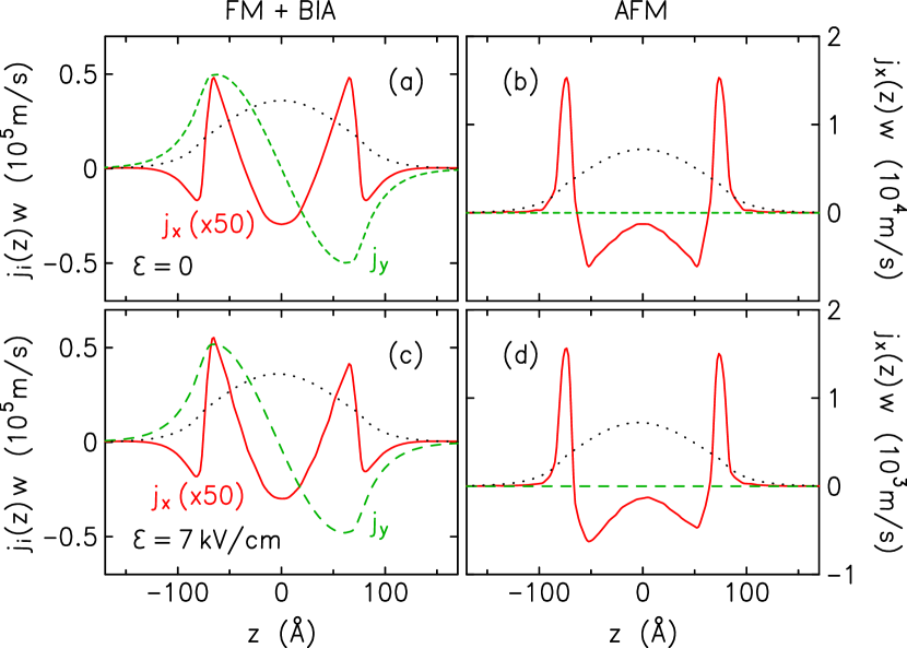
Figure 4: Equilibrium current distribution ${\bm{\mathrm{j}}}_{\|}(z)$ in a quantum well with width $w=150\,$Å, barrier height $V_{0}=0.12\,$eV, and electron density $N_{s}=1.0\times 10^{11}\,$cm^-2. Left column [panels (a), (c)]: Ferromagnetic InSb with $\mathcal{X}_{x}=8\,$meV and BIA. Right column [panels (b), (d)]: Diamond antiferromagnet with InSb band-structure parameters (without BIA) and $\mathcal{Y}_{x}=50\,$meV. Upper row [panels (a), (b)]: symmetric quantum well ($\mathcal{E}_{z}=0$). Lower row [panels (c), (d)]: tilted quantum well ($\mathcal{E}_{z}=7\,$kV/cm). In each panel, the dotted line shows for comparison the charge distribution $\rho(z)$ (arbitrary units). In both configurations (FM+BIA and AFM), the applied electric field distorts the, at zero field purely quadrupolar, equilibrium-current-density component $j_{x}$, thus inducing a finite magnetization in $y$ direction [Figs. 3(a) and 3(b)].

The matrix elements contributing to the second term in Eq. (39b) are nonzero independently of an electric field $\mathcal{E}_{z}$ (provided the product $\nu^{\prime}\nu$ is also even). For $\nu^{\prime}=2$, we get equilibrium currents proportional to $\phi_{0}(z)\phi_{2}(z)$ that give rise to a magnetic quadrupole ${\bm{\mathcal{Q}}}$ [Eq. (55) below]. The quadrupolar currents are illustrated in numerical calculations for a quantum well with finite barriers and using the more complete multiband Hamiltonian $\mathcal{H}$, see Figs. 4(a) and 4(c). The quadrupolar currents and the magnetic quadrupole ${\bm{\mathcal{Q}}}$ are indicative of orbital antiferromagnetic order that is induced parallel to the Zeeman field ${\bm{\mathcal{Z}}}$ by the interplay of ${\bm{\mathcal{Z}}}$, the Dresselhaus term (26c), and confinement [the potential $V(z)$]. The quadrupolar currents are odd both under spatial inversion and time inversion, consistent with the general discussion of antiferromagnetic order in Sec. IV.2 below. The orbital antiferromagnetic order can be quantified using the Néel operator ${\bm{\mathrm{\tau}}}$ defined below [Eq. (73)]. The Hamiltonian (28) (with $\mathcal{E}_{z}=0$) yields a nonzero expectation value

$$\braket{{\bm{\mathrm{\tau}}}}=2\pi\,q_{\tau}\,d\,N_{\mathrm{s}}\,\xi(\mathcal{Z})\begin{pmatrix}\cos\varphi_{\mathcal{Z}}\\ \sin\varphi_{\mathcal{Z}}\end{pmatrix}\sum_{\nu^{\prime}\neq 0}\frac{|\braket{\nu^{\prime}}{k_{z}^{2}}{0}|^{2}}{E_{0}^{(0)}-E_{\nu^{\prime}}^{(0)}}\;,$$ (41)

where we assumed, as before, that only the lowest subband $\nu=0$ is occupied. [Here $q_{\tau}$ is a band-structure parameter whose properties are discussed in greater detail below Eq. (73).] As we have $\braket{{\bm{\mathrm{\tau}}}}\parallel{\bm{\mathcal{Z}}}$ we can interpret such a scenario as ferrimagnetic order. This classification proposed here applies, in particular, to Mn-doped semiconductors such as GaMnAs and InMnSb . It is a peculiarity of an infinitely deep square well that ${\bm{\mathrm{\kappa}}}_{\nu^{\prime}\nu}\propto\delta_{\nu^{\prime}\nu}$ so that within this model we do not obtain quadrupolar equilibrium currents and orbital antiferromagnetic order.

The last term in Eq. (39b) (with $\nu^{\prime\prime}=1$) describes $\mathcal{E}_{z}$-induced dipolar currents that contribute to the magnetization [Fig. 4(c)]. For $\varphi_{\mathcal{Z}}=n\pi/2$ ($n$ integer), the quadrupolar and dipolar currents flow (anti)parallel to the field ${\bm{\mathcal{Z}}}$, consistent with Eq. (34). As to be expected, the total current ${\bm{\mathcal{J}}}_{\|}=\int dz\,{\bm{\mathcal{j}}}_{\|}(z)$ always vanishes. The fact that the coupling of the currents ${\bm{\mathcal{j}}}_{\|}(z)$ to a perpendicular electric field $\mathcal{E}_{z}$ is dissipationless resembles the Lorentz force. However, it needs to be emphasized that the equilibrium currents ${\bm{\mathcal{j}}}_{\|}(z)$ and their manipulation via electric fields are pure quantum effects with no classical analogue.

The numerical calculations for a ferromagnetic quantum well based on the multiband Hamiltonian $\mathcal{H}$ and presented in Figs. 4(a) and 4(c) assume that the exchange field ${\bm{\mathcal{X}}}_{\|}$ is oriented in $x$ direction. In this case, the equilibrium currents ${\bm{\mathcal{j}}}_{\|}(z)$ represented by Eq. (39b) are oriented likewise in $x$ direction. These currents are complemented by equilibrium currents $\mathcal{j}_{y}$ representing the orbital magnetization ${\bm{\mathcal{M}}}_{\mathcal{Z}}$ induced by the exchange field $\mathcal{X}_{z}$ and discussed in more detail in Appendix C.

III.3 $\mathcal{B}$-induced electric polarization

To calculate the equilibrium electric polarization induced by a magnetic field ${\bm{\mathcal{B}}}_{\|}$, we start again from the Hamiltonian (23). Specializing to $\mathcal{E}_{z}=0$ yields

$$\mathsf{H}_{{\bm{\mathcal{P}}}\leftarrow{\bm{\mathcal{B}}}}=\mathsf{H}^{(0)}+\mathsf{H}_{\mathcal{Z}}^{(0)}+\mathsf{H}_{\mathrm{D}}^{(1)}+\mathsf{H}_{\mathcal{B}}^{(1)}\,\,,$$ (42)

with $\mathsf{H}^{(0)}$, $\mathsf{H}_{\mathcal{Z}}^{(0)}$, and $\mathsf{H}_{\mathrm{D}}^{(1)}$ given by Eqs. (26a), (26b), and (26c), respectively, and [ignoring terms $\mathcal{O}(\mathcal{B}_{\|}^{2})$]

$$\mathsf{H}_{\mathcal{B}}^{(1)} =\frac{e\hbar}{2m}\left[\left({\bm{\mathrm{k}}}_{\|}-{\bm{\mathrm{k}}}_{0}\right)\cdot{\bm{\mathcal{A}}}+{\bm{\mathcal{A}}}\cdot\left({\bm{\mathrm{k}}}_{\|}-{\bm{\mathrm{k}}}_{0}\right)\right]\,\,,$$ (43a)

$$=\frac{e\hbar}{2m}\left[2\left({\bm{\mathrm{k}}}_{\|}-\lAngle\,{\bm{\mathrm{k}}}_{0}\,\rAngle\right)\cdot{\bm{\mathcal{A}}}-\left({\bm{\mathrm{k}}}_{0}-\lAngle\,{\bm{\mathrm{k}}}_{0}\,\rAngle\right)\cdot{\bm{\mathcal{A}}}-{\bm{\mathcal{A}}}\cdot\left({\bm{\mathrm{k}}}_{0}-\lAngle\,{\bm{\mathrm{k}}}_{0}\,\rAngle\right)\right]\,\,,$$ (43b)

$$=\frac{e\hbar}{m}\left({\bm{\mathrm{k}}}_{\|}-\lAngle\,{\bm{\mathrm{k}}}_{0}\,\rAngle\right)\cdot{\bm{\mathcal{A}}}-\frac{e}{\hbar}\,d\,\mathcal{B}_{\|}\left[\sin(\varphi_{\mathcal{Z}}+\varphi_{\mathcal{B}})\,\sigma_{z}+\cos(\varphi_{\mathcal{Z}}+\varphi_{\mathcal{B}})\,\sigma_{x}\right]\{z,k_{z}^{2}-\braket{k_{z}^{2}}\}\,\,,$$ (43c)

where $\varphi_{\mathcal{B}}$ is the angle between the direction of the applied magnetic field ${\bm{\mathcal{B}}}_{\|}$ and the $[100]$ crystallographic direction. The perturbation $\mathsf{H}_{\mathcal{B}}^{(1)}$ yields the perturbed states

$$\ket{\nu\sigma^{(1)}}=\ket{\nu\sigma}+\sum_{\sigma^{\prime},\nu^{\prime}\neq\nu}\frac{\Braket{\nu^{\prime}\sigma^{\prime}}{\mathsf{H}_{\mathcal{B}}^{(1)}}{\nu\sigma}}{E_{\nu}^{(0)}-E_{\nu^{\prime}}^{(0)}}\,\ket{\nu^{\prime}\sigma^{\prime}}\,\,.$$ (44)

We get

$$\lAngle\,z\,\rAngle =\braket{z}_{\nu\sigma}+2\sum_{\nu^{\prime}\neq\nu}c_{\nu^{\prime}\nu}\Braket{\nu\sigma}{\mathsf{H}_{\mathcal{B}}^{(1)}}{\nu^{\prime}\sigma}\,\,,$$ (45a)

$$=\braket{z}_{\nu\sigma}+2\sum_{\nu^{\prime}\neq\nu}c_{\nu^{\prime}\nu}\biggl{[}\frac{e\hbar}{m}({\bm{\mathrm{k}}}_{\|}-\lAngle\,{\bm{\mathrm{k}}}_{0}\,\rAngle)\cdot\braket{\nu}{{\bm{\mathcal{A}}}}{\nu^{\prime}}$$

$$\hskip 10.00002pt{}-\sigma\,\sin(\varphi_{\mathcal{Z}}+\varphi_{\mathcal{B}})\,\frac{e}{\hbar}\mathcal{d}\,\mathcal{B}_{\|}\,\braket{\nu}{\{z,k_{z}^{2}-\braket{k_{z}^{2}}\}}{\nu^{\prime}}\biggr{]}\,\,.$$ (45b)

Here, the first term $\braket{z}_{\nu\sigma}$ vanishes for a symmetric potential $V(z)$. The first term in the square brackets describes a ${\bm{\mathrm{k}}}_{\|}$-dependent shift [73, 74, 75, 76] that yields a vanishing contribution to $\mathcal{P}_{z}^{\mathrm{e}}$ when summed over the equilibrium Fermi sea. Therefore, a nonzero polarization is due to the second term in the square brackets, which yields a contribution independent of the wave vector ${\bm{\mathrm{k}}}_{\|}$. Summing over the Fermi sea, we obtain [69]

$$\mathcal{P}_{z}^{\mathrm{e}}=\mathcal{P}_{0}\,\,\mu_{\mathrm{B}}\mathcal{B}_{\|}\,\,\lambda_{d}\,\,\xi(\mathcal{Z})\,\,\sin(\varphi_{\mathcal{Z}}+\varphi_{\mathcal{B}})\,\,,$$ (46)

where $\lambda_{d}$ is given by Eq. (35). We see that the induced magnetoelectric effects are most pronounced when $\sin(\varphi_{\mathcal{Z}}+\varphi_{\mathcal{B}})=\pm 1\equiv\zeta$. This situation is realized in ferromagnetic systems when ${\bm{\mathcal{X}}}_{\|}\parallel{\bm{\mathrm{\hat{x}}}}\equiv[100]$ and ${\bm{\mathcal{B}}}_{\|}\parallel{\bm{\mathrm{\hat{y}}}}\equiv[010]$. Here the magnetization scales linearly with ${\bm{\mathcal{B}}}_{\|}$ [for $(g/2)\mu_{\mathrm{B}}\mathcal{B}_{\|}\ll\mathcal{X}$]. In paramagnetic systems with $\mathcal{X}=0$ and ${\bm{\mathcal{Z}}}=(g/2)\mu_{\mathrm{B}}{\bm{\mathcal{B}}}_{\|}$, we have $\zeta=\pm 1$ when ${\bm{\mathcal{B}}}_{\|}\parallel[110]$. In this case the polarization $\mathcal{P}_{z}^{\mathrm{e}}$ depends quadratically on ${\bm{\mathcal{B}}}_{\|}$, consistent with Eq. (2). Thus the system exhibits a higher-order magnetoelectric effect [29, 30] that is the nondissipative counterpart of the previously discussed magnetically induced electric polarization in a multi-quantum-well system [77, 78, 79]. Figure 3(c) illustrates the polarization (46) for a ferromagnetic InSb quantum well.

The mechanism for the ${\bm{\mathcal{B}}}$-induced polarization can be understood as follows: the vector potential ${\bm{\mathcal{A}}}$ of a magnetic field ${\bm{\mathcal{B}}}_{\|}$ has previously been used as a tool to manipulate the charge density $\rho(z)$ in quasi-2D systems such as semiconductor quantum wells. Ordinarily, a field ${\bm{\mathcal{B}}}_{\|}$ makes the charge distribution $\rho(z)$ bilayer-like by pushing $\rho(z)$ towards the barriers, but $\rho(z)$ still preserves the mirror symmetry of a symmetric quantum well [73, 74, 75, 76]. This effect stems from terms quadratic in ${\bm{\mathcal{A}}}$ that we have ignored in the above analytical model. In a low-symmetry configuration [indicated here by the presence of the Dresselhaus term $\mathsf{H}_{\mathrm{D}}$ given in Eq. (22c)], odd powers of the vector potential ${\bm{\mathcal{A}}}$ can change $\rho(z)$ in a way that no longer preserves the mirror symmetry of the confining potential $V(z)$. This effect resembles the Coulomb force, where the scalar potential is replaced by the vector potential ${\bm{\mathcal{A}}}$. However, it needs to be emphasized that, similar to Landau diamagnetism, we have here a pure quantum effect; it has no classical analogue. This effect is orbital in nature; it does not require a spin degree of freedom. For example, it exists also in spinless 2D hole systems that have a purely orbital Dresselhaus term.

III.4 Magnetoelectric contribution to the free energy

We evaluate the change $\delta F$ in the free-energy density due to the presence of both $\mathsf{H}_{\mathcal{E}}^{(1)}$ [Eq. (29)] and $\mathsf{H}_{\mathcal{B}}^{(1)}$ [Eq. (43c)] as

$$\delta F=\frac{1}{w}\sum_{\nu,\sigma}\int\frac{d^{2}k_{\|}}{(2\pi)^{2}}\;f(E_{\nu\sigma{\bm{\mathrm{k}}}_{\|}})\;\lAngle\,\mathsf{H}_{\mathcal{E}}^{(1)}+\mathsf{H}_{\mathcal{B}}^{(1)}\,\rAngle_{\nu\sigma{\bm{\mathrm{k}}}_{\|}}\,,$$ (47)

using second-order perturbation theory

$$\lAngle\,\mathsf{H}_{\mathcal{E}}^{(1)}+\mathsf{H}_{\mathcal{B}}^{(1)}\,\rAngle_{\nu\sigma{\bm{\mathrm{k}}}_{\|}} =2\Re\mathrm{e}\,\sum_{\nu^{\prime}\neq\nu}\frac{\braket{\nu}{\mathsf{H}_{\mathcal{E}}^{(1)}}{\nu^{\prime}}\braket{\nu^{\prime}}{\mathsf{H}_{\mathcal{B}}^{(1)}}{\nu}}{E_{\nu}^{(0)}-E_{\nu^{\prime}}^{(0)}}$$ (48a)

$$=2\Re\mathrm{e}\,\sum_{\nu^{\prime}\neq\nu}\frac{\braket{\nu}{e\mathcal{E}_{z}\,z}{\nu^{\prime}}\Braket{\nu^{\prime}}{\frac{e\hbar}{m}\left({\bm{\mathrm{k}}}_{\parallel}-\lAngle\,{\bm{\mathcal{k}}}_{0}\,\rAngle\right)\cdot{\bm{\mathcal{A}}}-\frac{e}{\hbar}\,\sigma\mathcal{d}\,\mathcal{B}_{\parallel}\,\sin(\varphi_{\mathcal{Z}}+\varphi_{\mathcal{B}})\,\{z,k_{z}^{2}-\braket{k_{z}^{2}}\}}{\nu}}{E_{\nu}^{(0)}-E_{\nu^{\prime}}^{(0)}}\;,$$ (48b)

where we ignored terms $\mathcal{O}(\mathcal{E}_{z}^{2})$ and $\mathcal{O}(\mathcal{B}_{\|}^{2})$. When averaging over all occupied states, the terms $\propto{\bm{\mathcal{A}}}$ drop out. Using Eq. (35), we get [69]

$$\delta F=N_{\mathrm{s}}\,\,e\mathcal{E}_{z}\,\,\mu_{\mathrm{B}}\mathcal{B}_{\|}\,\,\lambda_{d}\,\,\xi(\mathcal{Z})\,\sin(\varphi_{\mathcal{Z}}+\varphi_{\mathcal{B}})\;,$$ (49)

consistent with Eqs. (34) and (46). Hence, within the present model, we have $\mathcal{P}_{z}=\mathcal{P}_{z}^{\mathrm{e}}$ and ${\bm{\mathcal{M}}}_{\|}={\bm{\mathcal{M}}}_{\|}^{\mathrm{e}}$.

The expression (49) can be written as a sum of terms of the type appearing in the third line of the general expansion (I). More specifically, we find

$$\delta F=-\alpha_{zx}\,\mathcal{E}_{z}\mathcal{B}_{x}-\alpha_{zy}\,\mathcal{E}_{z}\mathcal{B}_{y}-\beta_{zxy}\,\mathcal{E}_{z}\mathcal{B}_{x}\mathcal{B}_{y}\quad,$$ (50a)

with

$${\bm{\mathrm{\alpha}}}_{z\|} \equiv \begin{pmatrix}\alpha_{zx}\\ \alpha_{zy}\end{pmatrix}=-e\mu_{\mathrm{B}}\,\lambda_{d}\times\left\{\!\begin{array}[]{@{}>{\Ds}cl@{}}\displaystyle\frac{m}{\pi\hbar^{2}}\,\mathcal{X}\begin{pmatrix}\sin\varphi_{\mathcal{X}}\\ \cos\varphi_{\mathcal{X}}\end{pmatrix},&\mathcal{Z}<E_{\mathrm{F}}^{0}\\[8.61108pt] \displaystyle N_{\mathrm{s}}\begin{pmatrix}\sin\varphi_{\mathcal{Z}}\\ \cos\varphi_{\mathcal{Z}}\end{pmatrix},&\mathcal{Z}\geq E_{\mathrm{F}}^{0}\end{array}\right.$$ (50d)

$$\beta_{zxy} = \left\{\begin{array}[]{>{\Ds}cl}\displaystyle-e\mu_{\mathrm{B}}^{2}\,\lambda_{d}\,\frac{gm}{\pi\hbar^{2}}\,,&\mathcal{Z}<E_{\mathrm{F}}^{0}\\[4.30554pt] \displaystyle 0\,,&\mathcal{Z}\geq E_{\mathrm{F}}^{0}\;.\end{array}\right.$$ (50h)

Clearly, $\alpha_{ij}\neq 0$ requires spontaneous ferromagnetic order due to a finite exchange field $\mathcal{X}_{\|}$ or full spin polarization (i.e., half-metallicity), and the particular form of the tensor $\alpha_{ij}$ with two nonzero entries $\alpha_{zx}$ and $\alpha_{zy}$ is consistent with the magnetic point group symmetry $22^{\prime}2^{\prime}$ of a ferromagnetic symmetric quantum well on a zincblende $(001)$ surface. A tensor $\alpha_{ij}\neq 0$ will generally also facilitate higher-order terms of the type $\propto\gamma_{ijk}$ in Eq. (I). In contrast, $\beta_{ijk}\neq 0$ occurs even in paramagnets, which is consistent with basic symmetry considerations [33, 29, 30, 34, 35] as zincblende structures allow for piezoelectricity.

The magnetoelectric contribution (49) to the free energy can also be expressed as [80]

$$\delta F=-\tilde{{\bm{\mathrm{\tau}}}}\cdot(\mathcal{E}_{z}\hat{{\bm{\mathrm{z}}}}\times{\bm{\mathcal{B}}}_{\|})$$ (51a)

in terms of a magnetoelectric vector

$$\tilde{{\bm{\mathrm{\tau}}}}=N_{\mathrm{s}}\,e\mu_{\mathrm{B}}\,\lambda_{d}\,\xi(\mathcal{Z})\begin{pmatrix}\cos\varphi_{\mathcal{Z}}\\ -\sin\varphi_{\mathcal{Z}}\end{pmatrix}\quad.$$ (51b)

The angular dependence of the magnetoelectric effect is governed by the orientation of the vector $\tilde{{\bm{\mathrm{\tau}}}}$, which in turn is determined by the orientation of the Zeeman field ${\bm{\mathcal{Z}}}$. In particular, there is a one-to-one correspondence between the orientation of the vector ${\bm{\mathcal{Z}}}$ in position space and the vector ${\bm{\mathrm{k}}}_{0}$ in reciprocal space; specifically the part ${\bm{\mathrm{k}}}_{0}^{(z)}$ of ${\bm{\mathrm{k}}}_{0}$ proportional to $\sigma_{z}$ that turned out to be relevant for the magnetoelectric effect in the above analysis. This vector ${\bm{\mathrm{k}}}_{0}^{(z)}$ is collinear with the vector $\tilde{{\bm{\mathrm{\tau}}}}$. Figure 5(a) shows the relation between the orientation of ${\bm{\mathcal{Z}}}$ and the orientation of $\tilde{{\bm{\mathrm{\tau}}}}$. A similar pattern exists for the current-induced spin magnetization (cf. Appendix A) in systems with Dresselhaus spin-orbit coupling (22c) for the orientation of the induced spin polarization as a function of the orientation of an in-plane electric field [66].

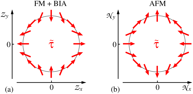
Figure 5: (a) Angular dependence of the orientation of the magnetoelectric vector $\tilde{{\bm{\mathrm{\tau}}}}$ [Eq. (51)] on the orientation of the Zeeman field ${\bm{\mathcal{Z}}}$ in ferromagnets with BIA. (b) Angular dependence of the orientation of the magnetoelectric vector $\tilde{{\bm{\mathrm{\tau}}}}$ [Eq. (92)], which is parallel to the vector $-{\bm{\mathcal{k}}}_{0}$ [Eq. (71)], on the orientation of the Néel vector ${\bm{\mathcal{N}}}$. The orientation of $\tilde{{\bm{\mathrm{\tau}}}}$ in (b) is antiparallel to the orientation of $\tilde{{\bm{\mathrm{\tau}}}}$ in (a) [81].

The vector $\mathcal{E}_{z}\hat{{\bm{\mathrm{z}}}}\times{\bm{\mathcal{B}}}_{\|}$ in Eq. (51a) is a toroidal vector, i.e., it is odd under both space inversion and time reversal [82]. On the other hand, Eq. (51b) shows that the vector $\tilde{{\bm{\mathrm{\tau}}}}$ transforms like a magnetic field, i.e., it is even under space inversion and odd under time reversal. The different transformational properties of the vectors $\mathcal{E}_{z}\hat{{\bm{\mathrm{z}}}}\times{\bm{\mathcal{B}}}_{\|}$ and $\tilde{{\bm{\mathrm{\tau}}}}$ in Eq. (51a) reflect the broken space-inversion symmetry in a zincblende structure.

The term $\delta F\propto\mathcal{E}_{z}\,\mathcal{B}_{\|}$ in Eq. (49) is generally complemented by a second magnetoelectric term $\propto\mathcal{E}_{z}\,\mathcal{B}_{\|}$. This is because the Hamiltonian $\mathsf{H}$ also includes a term

$$\mathsf{H}_{\mathcal{EB}}=b\,e\mathcal{E}_{z}\,\mu_{\mathrm{B}}(\mathcal{B}_{x}\sigma_{y}+\mathcal{B}_{y}\sigma_{x})\;,$$ (52)

characterizing the bulk zincblende structure that underlies the quasi-2D systems studied here. The prefactor $b$ is given in Eq. (7.5) of Ref. [66] in terms of momentum matrix elements and energy gaps appearing in the larger Hamiltonian $\mathcal{H}$, yielding $b=-221\,$Å/eV for InSb and $-1.36\,$Å/eV for GaAs. The term (52) produces a second magnetoelectric term in the free energy,

$$\delta F_{\mathrm{bulk}}=N_{\mathrm{s}}\,\,e\mathcal{E}_{z}\,\,\mu_{\mathrm{B}}\mathcal{B}_{\|}\,\frac{b}{w}\,\,\xi(\mathcal{Z})\,\sin(\varphi_{\mathcal{Z}}+\varphi_{\mathcal{B}})\;,$$ (53)

that complements $\delta F$ in Eq. (49). Their ratio is given by

$$\left|\frac{\delta F_{\mathrm{bulk}}}{\delta F}\right|\equiv\left|\frac{b}{w\lambda_{d}}\right|=\frac{6\pi^{2}}{\pi^{2}-6}\,\frac{\hbar^{2}b}{mw^{2}l_{d}}\;,$$ (54)

where the expression on the far r.h.s. of Eq. (54) is obtained using Eq. (35) for a hard-wall confinement $V(z)$. This ratio evaluates to $9300/(w[\mathrm{\AA}])^{2}$ in InSb and $330/(w[\mathrm{\AA}])^{2}$ in GaAs, and it is consequently much smaller than $1$ for typical quantum-well widths $w\gtrsim 150\,$Å. Experimental signatures of an $\mathcal{E}_{z}\,\mathcal{B}_{\|}$-type magnetoelectric coupling have recently been observed for charge carriers in deformed donor bound states [83].

III.5 Magnetic quadrupole moment

The magnetoelectric tensor $\alpha_{ij}$ behaves under symmetry transformations like a magnetic quadrupole moment [50], i.e., both of these second-rank material tensors require broken space-inversion symmetry and broken time-reversal symmetry and these tensors share the same pattern of nonzero components. Similar to the magnetization ${\bm{\mathcal{M}}}=-\partial F/\partial{\bm{\mathcal{B}}}$, the components of the magnetic quadrupole moment can be obtained from the free energy density $F$ via the relations [84]

$$\mathcal{Q}_{ij}=-2\frac{\partial F}{\partial(\nabla_{i}\mathcal{B}_{j})}\;,$$ (55)

where $\nabla_{i}\mathcal{B}_{j}$ denotes field gradients. [Note that, for the purpose of discussing the magnetic quadrupole moment, ${\bm{\mathcal{B}}}_{\|}\equiv{\bm{\mathcal{B}}}_{\|}({\bm{\mathrm{r}}})$ necessarily denotes an inhomogeneous magnetic field, in contrast to the other parts of this Article where ${\bm{\mathcal{B}}}_{\|}$ is assumed to be homogeneous.] For the quasi-2D systems studied here, $\mathcal{Q}_{ij}$ is the sum of two contributions

$$\mathcal{Q}_{ij}=\mathcal{Q}_{ij}^{\mathrm{e}}+\mathcal{Q}_{ij}^{\mathrm{q}}\,\,,$$ (56)

with

$$\mathcal{Q}_{ij}^{\mathrm{e}} =-\frac{2}{w}\sum_{n}\int\frac{d^{2}k_{\|}}{(2\pi)^{2}}\;f(E_{n{\bm{\mathrm{k}}}_{\|}})\,\frac{\partial E_{n{\bm{\mathrm{k}}}_{\|}}}{\partial(\nabla_{i}\mathcal{B}_{j})}\;,$$ (57a)

$$\mathcal{Q}_{ij}^{\mathrm{q}} =-\frac{2}{w}\sum_{n}\int\frac{d^{2}k_{\|}}{(2\pi)^{2}}\;E_{n{\bm{\mathrm{k}}}_{\|}}\,\frac{\partial f(E_{n{\bm{\mathrm{k}}}_{\|}})}{\partial(\nabla_{i}\mathcal{B}_{j})}\;,$$ (57b)

that represent the electromagnetic and the quantum-kinetic effects of the field gradients $\nabla_{i}\mathcal{B}_{j}$, respectively. Given that ${\bm{\mathcal{B}}}_{\|}$ generally enters the Hamiltonian $H$ via both the vector potential ${\bm{\mathcal{A}}}$ and also via the Zeeman term, the contribution $\mathcal{Q}_{ij}^{\mathrm{e}}$ can be split further into orbital and spin contributions,

$$\mathcal{Q}_{ij}^{\mathrm{e}}=\mathcal{Q}_{ij}^{\mathrm{o}}+\mathcal{Q}_{ij}^{\mathrm{s}}\;,$$ (58)

where the spin quadrupole moment

$$\mathcal{Q}_{ij}^{\mathrm{s}}=-\frac{2}{w}\sum_{n}\int\frac{d^{2}k_{\|}}{(2\pi)^{2}}\;f(E_{n{\bm{\mathrm{k}}}_{\|}})\,\Big{\langle}\frac{\partial H}{\partial(\nabla_{i}\mathcal{B}_{j})}\Big{\rangle}_{n{\bm{\mathrm{k}}}_{\|}}$$ (59)

vanishes for the Hamiltonian (22) studied here. For the orbital part

$$\mathcal{Q}_{ij}^{\mathrm{o}}=-\frac{2}{w}\sum_{n}\!\int\!\frac{d^{2}k_{\|}}{(2\pi)^{2}}\,f(E_{n{\bm{\mathrm{k}}}_{\|}})\,\Big{\langle}\sum_{l=x,y}\frac{\partial H}{\partial\mathcal{A}_{l}}\frac{\partial\mathcal{A}_{l}}{\partial(\nabla_{i}\mathcal{B}_{j})}\Big{\rangle}_{n{\bm{\mathrm{k}}}_{\|}},$$ (60)

we consider the inhomogenous magnetic field to have the particular form

$${\bm{\mathcal{B}}}_{\|}(z)={\bm{\mathcal{B}}}_{\|}^{0}+z\,{\bm{\mathcal{b}}}_{\|}$$ (61)

with constant vectors ${\bm{\mathcal{B}}}_{\|}^{0}$ and ${\bm{\mathcal{b}}}_{\|}$, so that $\nabla_{z}{\bm{\mathcal{B}}}_{\|}={\bm{\mathcal{b}}}_{\|}$, and we choose the vector potential

$${\bm{\mathcal{A}}}=\bigl{(}z\,{\bm{\mathcal{B}}}_{\|}^{0}+{\textstyle\frac{1}{2}}\,z^{2}\,{\bm{\mathcal{b}}}_{\|}\bigr{)}\times\hat{{\bm{\mathrm{z}}}}\;.$$ (62)

Similar to the discussion in Appendix B, this gauge yields for the components $(\mathcal{Q}_{zx}^{\mathrm{o}},\mathcal{Q}_{zy}^{\mathrm{o}})\equiv{\bm{\mathcal{Q}}}_{z\|}^{\mathrm{o}}$ of the orbital quadrupole moment

$${\bm{\mathcal{Q}}}_{z\|}^{\mathrm{o}}=-\frac{e}{w}\sum_{n}\int\frac{d^{2}k_{\|}}{(2\pi)^{2}}\,\,f(E_{n{\bm{\mathrm{k}}}_{\|}})\,\hat{{\bm{\mathrm{z}}}}\times\braket{\{z^{2}\,,{\bm{\mathrm{v}}}}{({\bm{\mathrm{k}}}}{)\}}_{n{\bm{\mathrm{k}}}_{\|}}\,.$$ (63)

Similar to the polarization $\mathcal{P}_{z}$ and magnetization ${\bm{\mathcal{M}}}_{\|}$ discussed in Sec. II, the orbital quadrupole moment (63) avoids the technical problems arising for these quantities in bulk (3D) systems. The orbital quadrupole moment in 3D systems has recently been discussed in Ref. [52].

We evaluate the matrix elements $\braket{\{z^{2}\,,{\bm{\mathrm{v}}}}{({\bm{\mathrm{k}}}}{)\}}$ similar to Eq. (33). We get in first order perturbation theory

$$\braket{\{z^{2}\,,{\bm{\mathrm{v}}}}{({\bm{\mathrm{k}}}}{)\}} =\braket{z^{2}}\braket{{\bm{\mathrm{v}}}}{({\bm{\mathrm{k}}}}{)}+\left(\braket{\{z^{2},{\bm{\mathrm{v}}}}{({\bm{\mathrm{k}}}}{)\}}-\braket{z^{2}}\braket{{\bm{\mathrm{v}}}}{({\bm{\mathrm{k}}}}{)}\right)$$ (64a)

$$=\braket{z^{2}}\braket{{\bm{\mathrm{v}}}}{({\bm{\mathrm{k}}}}{)}-\frac{\hbar}{m}\bigl{(}\braket{\{z^{2},{\bm{\mathrm{k}}}_{0}\}}-\braket{z^{2}}\braket{{\bm{\mathrm{k}}}_{0}}\bigr{)}$$ (64b)

$$=\braket{z^{2}}\braket{{\bm{\mathrm{v}}}}{({\bm{\mathrm{k}}}}{)}-\frac{d}{\hbar}\left[\begin{pmatrix}\cos\varphi_{\mathcal{Z}}\\ -\sin\varphi_{\mathcal{Z}}\end{pmatrix}\braket{\{z^{2},k_{z}^{2}-\braket{k_{z}^{2}}\}\,\sigma_{z}}-\begin{pmatrix}\sin\varphi_{\mathcal{Z}}\\ \cos\varphi_{\mathcal{Z}}\end{pmatrix}\braket{\{z^{2},k_{z}^{2}-\braket{k_{z}^{2}}\}\,\sigma_{x}}\right]$$ (64c)

$$=\braket{z^{2}}\braket{{\bm{\mathrm{v}}}}{({\bm{\mathrm{k}}}}{)}-\sigma\frac{d}{\hbar}\begin{pmatrix}\cos\varphi_{\mathcal{Z}}\\ -\sin\varphi_{\mathcal{Z}}\end{pmatrix}\braket{\{z^{2},k_{z}^{2}-\braket{k_{z}^{2}}\}}\;.$$ (64d)

In the last step, we kept only terms linear in the Dresselhaus coefficient $d$. The first term in Eq. (64d) yields a vanishing contribution when summed over the equilibrium Fermi sea, as it is proportional to the system’s total equilibrium current. Therefore, a nonzero quadrupole moment is due to the second term in Eq. (64d), which yields a contribution independent of the wave vector ${\bm{\mathrm{k}}}_{\|}$. Consistent with the above discussion of equilibrium currents, we have $\braket{\{z^{2},k_{z}^{2}-\braket{k_{z}^{2}}\}}=0$ for an infinitely deep square well and $\braket{\{z^{2},k_{z}^{2}-\braket{k_{z}^{2}}\}}=-\nu-\frac{1}{2}$ for the $\nu$th subband in a harmonic-oscillator potential. Summing over the Fermi sea and assuming a small density $N_{\mathrm{s}}$ such that only the lowest subband $\nu=0$ is occupied, we obtain

$${\bm{\mathcal{Q}}}_{z\|}^{\mathrm{o}}=\mathcal{Q}_{0}\,\,\frac{l_{d}}{w}\,\braket{\{z^{2},k_{z}^{2}-\braket{k_{z}^{2}}\}}\,\,\xi(\mathcal{Z})\begin{pmatrix}\sin\varphi_{\mathcal{Z}}\\ \cos\varphi_{\mathcal{Z}}\end{pmatrix}\,\,,$$ (65)

with $\mathcal{Q}_{0}=-\mu_{\mathrm{B}}N_{\mathrm{s}}$. The quadrupole moment ${\bm{\mathcal{Q}}}_{z\|}^{\mathrm{o}}$ shows the same dependence on the orientation of the Zeeman field ${\bm{\mathcal{Z}}}$ as the magnetization ${\bm{\mathcal{M}}}_{\|}^{\mathrm{o}}$ [Eq. (34)], where ${\bm{\mathcal{Z}}}$ may be due to an exchange field ${\bm{\mathcal{X}}}_{\|}$ or due to an external field ${\bm{\mathcal{B}}}_{\|}$. On the other hand, the vector ${\bm{\mathcal{Q}}}_{z\|}^{\mathrm{o}}$ shows a different dependence on the orientation of ${\bm{\mathcal{Z}}}$ than is exhibited by the expectation value (41) of the Néel operator ${\bm{\mathrm{\tau}}}$. This is similar to how a spin magnetization ${\bm{\mathcal{S}}}$ and the spin polarization $\braket{{\bm{\mathrm{\sigma}}}}$ can show different dependences on the orientation of an external magnetic field ${\bm{\mathcal{B}}}$ when the Zeeman coupling in the field ${\bm{\mathcal{B}}}$ is characterized by a $g$ tensor. See Eq. (16b) and Ref. [85].

Alternatively, we can obtain the result (65) by evaluating the free energy $F$ in the presence of the vector potential ${\bm{\mathcal{A}}}$ for the field gradient ${\bm{\mathcal{b}}}_{\|}$. To first order in ${\bm{\mathcal{b}}}_{\|}$ and the Dresselhaus coefficient $d$, we get an energy shift of the occupied states given by the expectation value of

$$H_{\mathcal{b}}^{(1)}=\frac{e\hbar}{m}\left({\bm{\mathrm{k}}}_{\|}-\braket{{\bm{\mathrm{k}}}_{0}}\right)\cdot{\bm{\mathcal{A}}}-\frac{e}{\hbar}\,d\,\frac{\mathcal{b}_{\|}}{2}\left[\sin(\varphi_{\mathcal{Z}}+\varphi_{\mathcal{b}})\,\sigma_{z}+\cos(\varphi_{\mathcal{Z}}+\varphi_{\mathcal{b}})\,\sigma_{x}\right]\{z^{2},k_{z}^{2}-\braket{k_{z}^{2}}\}\,\,,$$ (66)

where $\varphi_{\mathcal{b}}$ is the angle between the direction of the field gradient ${\bm{\mathcal{b}}}_{\|}$ and the $[100]$ crystallographic direction; compare Eq. (43). When averaging over all occupied states, the first term $\propto{\bm{\mathcal{A}}}$ drops out. We get

$$\delta F=-\mathcal{Q}_{0}\,\frac{\mathcal{b}_{\|}}{2}\,\frac{l_{d}}{w}\braket{\{z^{2},k_{z}^{2}-\braket{k_{z}^{2}}\}}\,\xi(\mathcal{Z})\,\sin(\varphi_{\mathcal{Z}}+\varphi_{\mathcal{b}})\,,$$ (67)

consistent with Eqs. (55) and (65).

The contribution (67) to the free energy can also be expressed as [80]

$$\delta F=-\bar{{\bm{\mathrm{\tau}}}}\cdot({\bm{\mathrm{\nabla}}}_{\!z}\times{\bm{\mathcal{B}}}_{\|})$$ (68a)

in terms of a vector

$$\bar{{\bm{\mathrm{\tau}}}}=\mathcal{Q}_{0}\,\frac{l_{d}}{2w}\braket{\{z^{2},k_{z}^{2}-\braket{k_{z}^{2}}\}}\,\xi(\mathcal{Z})\begin{pmatrix}-\cos\varphi_{\mathcal{Z}}\\ \sin\varphi_{\mathcal{Z}}\end{pmatrix}$$ (68b)

that characterizes the orientation of the magnetic quadrupole, similar to how the angular dependence of the magnetoelectric effect is governed by the orientation of the vector $\tilde{{\bm{\mathrm{\tau}}}}$, compare Eq. (51).

It has recently been suggested [51, 52, 86] that the components $\mathcal{Q}_{ij}$ of the magnetic quadrupole moment are connected with the components $\alpha_{ij}$ of the magnetoelectric tensor via the relation $e\,\partial\mathcal{Q}_{ij}/\partial\mu=-\alpha_{ij}$, where $\mu$ is the chemical potential. For the metallic quasi-2D systems studied here, this relation is fulfilled neither for an infinitely deep square well, where $\mathcal{Q}_{ij}=0$ but $\alpha_{ij}\neq 0$, nor for a parabolic well, where $\mathcal{Q}_{ij}\neq 0$ but $\alpha_{ij}=0$. The magnetic quadrupole moment is found to arise solely from the energy change of the confined-charge-carrier states due to the magnetic-field gradient ${\bm{\mathcal{b}}}_{\|}$ obtained by first-order perturbation theory [Eq. (67)]; it has none of the additional contributions derived for bulk systems [86]. On the other hand, the magnetoelectric tensor $\alpha_{ij}$ requires second-order perturbation theory for two perturbations ${\bm{\mathcal{E}}}$ and ${\bm{\mathcal{B}}}$, see, e.g., Eq. (47) and Ref. [50]. These results suggest that $\mathcal{Q}_{ij}$ and $\alpha_{ij}$ should generally be viewed as independent coefficients in a Taylor expansion of the free energy $F$ as a function of the external fields ${\bm{\mathcal{E}}}$ and ${\bm{\mathcal{B}}}$.

III.6 Magnetoelectricity in ferromagnetic hole systems

The magnetoelectric response obtained in the realistic calculations for electron systems in ferromagnetic InSb quantum wells is small [Figs. 3(a) and 3(c)]. The response can be greatly enhanced by a suitable engineering of the band structure $E_{n{\bm{\mathrm{k}}}_{\|}}$ of the quasi-2D systems. Here quasi-2D hole systems have long been known as a versatile playground for bandstructure engineering, where the dispersion of the first heavy-hole (HH) subband is strongly affected by the coupling to the first light-hole (LH) subband [87, 88, 66]. Figures 6(a) and 6(d) illustrate this for quasi-2D hole systems in paramagnetic InSb quantum wells with width $w=150\,$Å [Fig. 6(a)] and $w=300\,$Å [Fig. 6(d)], where HH-LH coupling results in a highly nonparabolic dispersion $E_{0{\bm{\mathrm{k}}}_{\|}}$ of the doubly degenerate ground HH subband. Furthermore, the dispersion is also highly anisotropic, which reflects the cubic symmetry of the underlying crystal structure.

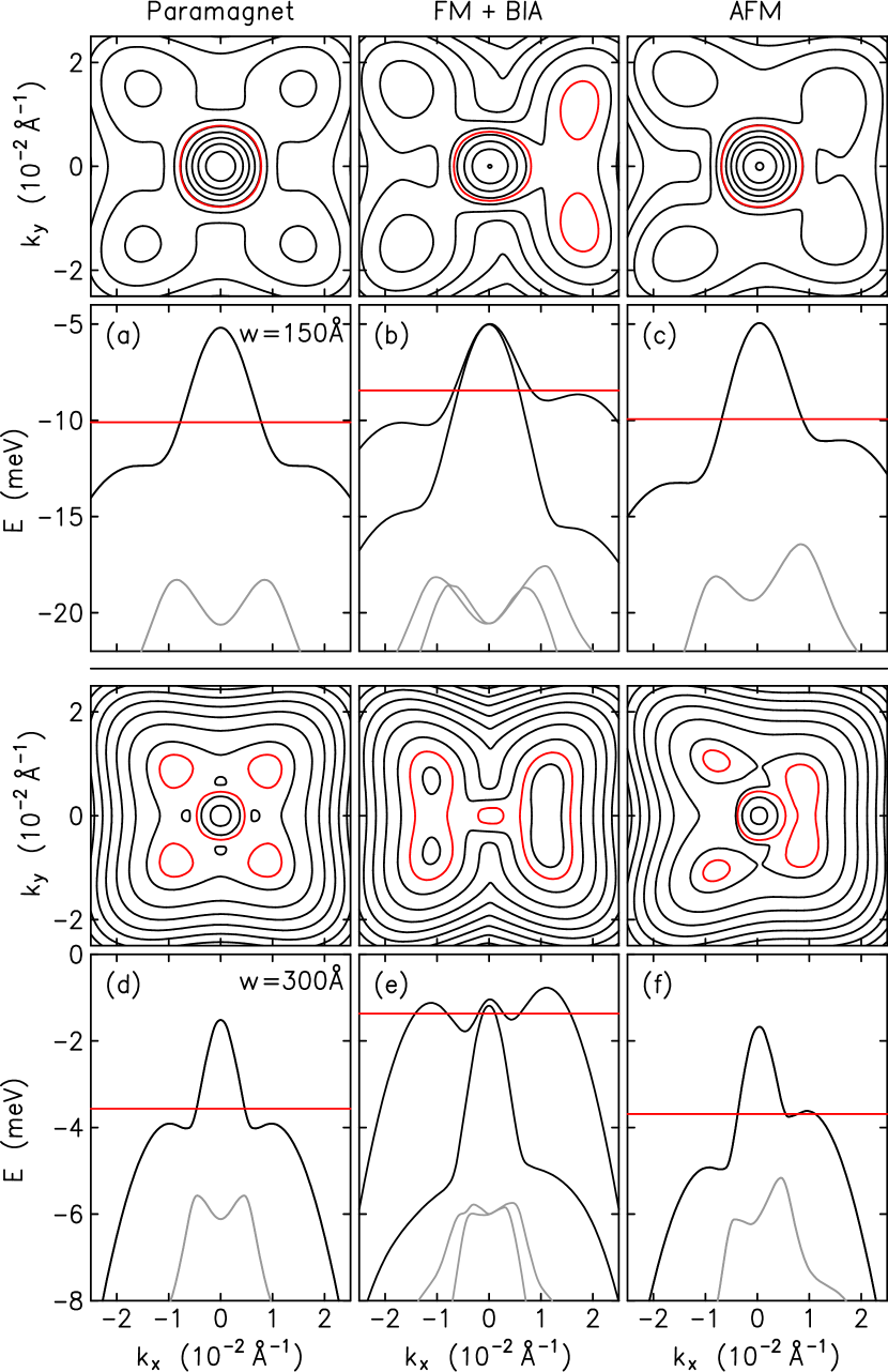
Figure 6: Subband dispersion (lower panels) of the HH subband (black) and LH subband (gray) of a quantum well with barrier height $V_{0}=0.12\,$eV, width $w=150\,$Å [upper row (a), (b), (c)] and $w=300\,$Å [lower row (d), (e), (f)] for $\mathcal{E}_{z}=\mathcal{B}_{\|}=0$. The upper panels show contour plots of the same dispersion with line increments of 0.1 meV. Red lines indicate the Fermi energy (lower panels) [Fermi contour (upper panels)] for a hole density $N_{s}=1.0\times 10^{11}\,$cm^-2. Left column [panels (a), (d)]: Paramagnetic InSb ignoring BIA. Center column [panels (b), (e)]: Ferromagnetic InSb with $\mathcal{X}_{x}=8\,$meV and BIA. Right column [panels (c), (f)]: Diamond antiferromagnet with InSb band-structure parameters (without BIA) and $\mathcal{Y}_{x}=50\,$meV.

An important aspect for the magnetoelectric response is the breaking of time-reversal symmetry so that $E_{n,-{\bm{\mathrm{k}}}_{\|}}\neq E_{n{\bm{\mathrm{k}}}_{\|}}$. The interplay between a ferromagnetic exchange field ${\bm{\mathcal{X}}}_{\|}$ and HH-LH coupling can result in a highly asymmetric band structure of quasi-2D HH systems with multiple disconnected parts of the Fermi surface, as illustrated in Figs. 6(b) and 6(e) for ferromagnetic InSb quantum wells [65]. Figures 7(a) and 7(c) exemplify the $\mathcal{E}_{z}$-induced orbital magnetic moment per particle, which can rise as high as $\sim 1\,\mu_{\mathrm{B}}$ for moderate electric fields $\mathcal{E}_{z}$. Figures 8(a), 8(c), 8(e), and 8(g) show the equilibrium currents. Finally, Figs. 9(a) and 9(c) show the ${\bm{\mathcal{B}}}_{\|}$-induced displacement $\braket{z}$ that represents the electrostatic polarization via Eq. (12).

The large magnetoelectric response of quasi-2D hole systems can be ascribed to the strong asymmetry $E_{n,-{\bm{\mathrm{k}}}_{\|}}\neq E_{n{\bm{\mathrm{k}}}_{\|}}$ of the band structure. With increasing fields, the disconnected parts of the Fermi sea that are located away from ${\bm{\mathrm{k}}}_{\|}={\bm{\mathrm{0}}}$ get depopulated and eventually disappear. The field-induced response drops again when finally only the central part of the Fermi sea around ${\bm{\mathrm{k}}}_{\|}={\bm{\mathrm{0}}}$ accommodates all charge carriers. Thus, unlike the electron case discussed above, the hole systems show a strongly nonlinear dependence of the magnetoelectric response as a function of the applied fields.

Figure 7: $\mathcal{E}_{z}$-induced orbital magnetic moment per particle $\mu_{\mathrm{B}}M_{y}^{\mathrm{o}}$ in a quantum well with barrier height $V_{0}=0.12\,$eV, width $w=150\,$Å [upper row (a), (b)] and $w=300\,$Å [lower row (c), (d)] and hole density $N_{s}=1.0\times 10^{11}\,$cm^-2. Left column [panels (a), (c)]: Ferromagnetic InSb with $\mathcal{X}_{x}=8\,$meV and BIA. Right column [panels (b), (d)]: Diamond antiferromagnet with InSb band-structure parameters (without BIA) and $\mathcal{Y}_{x}=50\,$meV.

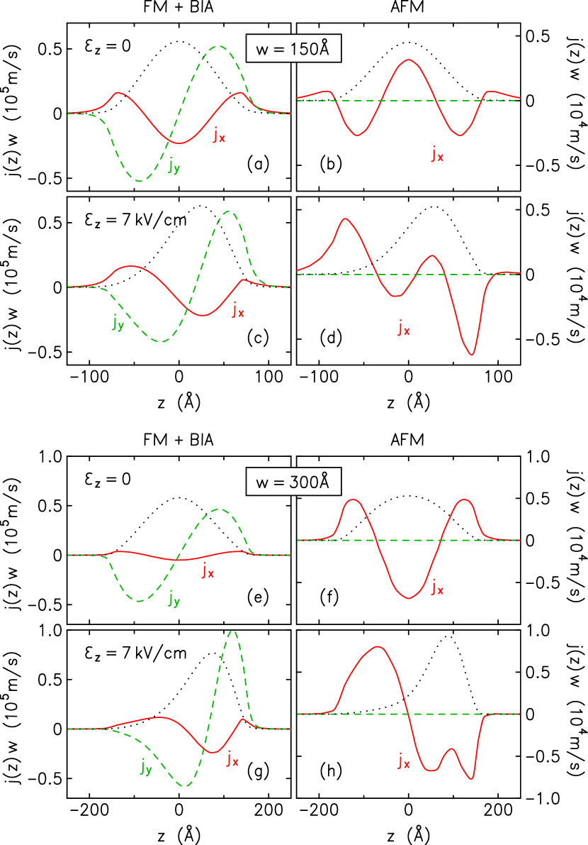
Figure 8: Equilibrium current distribution ${\bm{\mathrm{j}}}_{\|}(z)$ in a quantum well with barrier height $V_{0}=0.12\,$eV, width $w=150\,$Å [panels (a), (b), (c), (d)] and $w=300\,$Å [panels (e), (f), (g), (h)] and hole density $N_{s}=1.0\times 10^{11}\,$cm^-2. Left column [panels (a), (c), (e), (g)]: Ferromagnetic InSb with $\mathcal{X}_{x}=8\,$meV and BIA. Right column [panels (b), (d), (f), (h)]: Diamond antiferromagnet with InSb band-structure parameters (without BIA) and $\mathcal{Y}_{x}=50\,$meV. Panels (a), (b), (e), (f): symmetric quantum well ($\mathcal{E}_{z}=0$). Panels (c), (d), (g), (h): tilted quantum well ($\mathcal{E}_{z}=7\,$kV/cm). In each panel, the dotted line shows for comparison the charge distribution $\rho(z)$ (arbitrary units).

Figure 9: $\mathcal{B}_{y}$-induced displacement $\braket{z}$ representing the electrostatic polarization via Eq. (12) in a quantum well with barrier height $V_{0}=0.12\,$eV, width $w=150\,$Å [upper row (a), (b)] and $w=300\,$Å [lower row (c), (d)] and hole density $N_{s}=1.0\times 10^{11}\,$cm^-2. Left column [panels (a), (c)]: Ferromagnetic InSb with $\mathcal{X}_{x}=8\,$meV and BIA. Right column [panels (b), (d)]: Diamond antiferromagnet with InSb band-structure parameters (without BIA) and $\mathcal{Y}_{x}=50\,$meV.

IV Magnetoelectricity in diamond antiferromagnets

Space-inversion symmetry of a diamond structure is broken in the zincblende structure [Figs. 1(a) and 1(b)]. Opposite magnetic moments placed alternatingly on the atomic sites of a diamond structure result in an antiferromagnetic structure [Fig. 1(c)]. Both time reversal $\Theta$ and space inversion $I$ are broken symmetries in such a diamond antiferromagnet. The joint operation $\Theta I$, however, remains a good symmetry so that, similar to paramagnetic diamond, a two-fold spin degeneracy is preserved throughout the Brillouin zone. Nonetheless, as these symmetries are broken individually, invariants proportional to the Néel vector ${\bm{\mathcal{N}}}$ appear in the Kane Hamiltonian that are forbidden in paramagnetic systems because of time-reversal symmetry. These invariants are derived in Sec. IV.1.

The diamond structure is realized by the A atoms of intermetallic cubic (C-15) Laves phases AB₂, and it has been demonstrated that NpCo₂ is an itinerant antiferromagnet, where the magnetic moments on the Np atoms are ordered as shown in Fig. 1(c) (magnetic space group $I4_{1}{}^{\prime}/a^{\prime}m^{\prime}d$) [89, 90]. The diamond structure is also realized by the A atoms of spinels AB₂X₄. Frequently, spinels with magnetic A atoms give rise to highly frustrated magnetic order [91]. Beyond that, a recent study combining experiment and theory [92] identified CoRh₂O₄ as a canonical diamond-structure antiferromagnet, where the magnetic moments on the Co atoms are ordered as shown in Fig. 1(c).

IV.1 The model

Our goal is to incorporate the effect of antiferromagnetic order into the ${\bm{\mathrm{k}}}\cdot{\bm{\mathrm{p}}}$ envelope-function theory [93, 66] underlying multiband Hamiltonians as in Eq. (21). To this end, we start from the well-known $sp^{3}$ tight-binding model for diamond and zincblende structures with spin-orbit coupling included [94, 95]. This model includes the $s$-bonding valence band $\Gamma_{6}^{v}$, the $p$-bonding valence bands $\Gamma_{8}^{v}$ and $\Gamma_{7}^{v}$, the $s$-antibonding conduction band $\Gamma_{6}^{c}$, and the $p$-antibonding conduction bands $\Gamma_{8}^{c}$ and $\Gamma_{7}^{c}$. Except for the low-lying valence band $\Gamma_{6}^{v}$, these bands are also the basis states for the $14\times 14$ extended Kane model [96, 66].

We add a staggered exchange field ${\bm{\mathcal{Y}}}$ on the two sublattices of the diamond structure as depicted in Fig. 1(c). Using the phase conventions for the basis functions of $\mathcal{H}$ that are described in detail in Appendix C of Ref. [66], the field ${\bm{\mathcal{Y}}}$ yields terms in the off-diagonal blocks $\mathcal{H}_{8c\,8v}^{\,}$, $\mathcal{H}_{8c\,7v}^{\,}$, and $\mathcal{H}_{7c\,7v}^{\,}$ of $\mathcal{H}$ that are listed in Table 2 using the notation of Table C.5 in Ref. [66]. The vector ${\bm{\mathcal{N}}}$ denotes the Néel unit vector with components $\mathcal{N}_{i}=\mathcal{Y}_{i}/\mathcal{Y}$. Within the $14\times 14$ extended Kane model, the off-diagonal invariants $\mathcal{H}_{8c\,8v}^{\,\mathcal{Y}}$, $\mathcal{H}_{8c\,7v}^{\,\mathcal{Y}}$, and $\mathcal{H}_{7c\,7v}^{\,\mathcal{Y}}$ provide a complete account of the antiferromagnetic order shown in Fig. 1(c).

The off-diagonal invariants $\mathcal{H}_{8c\,8v}^{\,\mathcal{Y}}$, $\mathcal{H}_{8c\,7v}^{\,\mathcal{Y}}$, and $\mathcal{H}_{7c\,7v}^{\,\mathcal{Y}}$ appear already for ${\bm{\mathrm{k}}}={\bm{\mathrm{0}}}$. In the diagonal blocks $\mathcal{H}_{6c\,6c}^{\,}$, $\mathcal{H}_{8v\,8v}^{\,}$, and $\mathcal{H}_{7v\,7v}^{\,}$, a Taylor expansion of the tight-binding Hamiltonian about ${\bm{\mathrm{k}}}={\bm{\mathrm{0}}}$ yields mixed terms proportional to powers of components of ${\bm{\mathcal{Y}}}$ and powers of components of ${\bm{\mathrm{k}}}$. The lowest-order invariants obtained in this way are also listed in Table 2. Alternatively, these terms can be derived by means of quasi-degenerate perturbation theory [66] applied to $\mathcal{H}$ with $\mathcal{H}_{8c\,8v}^{\,\mathcal{Y}}$, $\mathcal{H}_{8c\,7v}^{\,\mathcal{Y}}$, and $\mathcal{H}_{7c\,7v}^{\,\mathcal{Y}}$ included. The latter approach yields explicit, albeit lengthy, expressions for the prefactors $\mathcal{d}$ and $\mathcal{D}^{i}_{jj}$ as a function of $\mathcal{Y}=|{\bm{\mathcal{Y}}}|$ that are omitted here. As to be expected for antiferromagnetic diamond, the ${\bm{\mathcal{Y}}}$-dependent invariants in Table 2 break time-reversal symmetry, but they do not lift the spin degeneracy. Using quasi-degenerate perturbation theory, we also obtain several invariants in the valence band block $\mathcal{H}_{8v\,8v}^{\,\mathcal{Y}}$ that are proportional to both ${\bm{\mathcal{Y}}}$ and an external electric field ${\bm{\mathcal{E}}}$. These invariants are listed in Table 2 as well. They describe a spin splitting proportional to the field ${\bm{\mathcal{E}}}$ (but independent of the wave vector ${\bm{\mathrm{k}}}$) that is induced by the antiferromagnetic exchange coupling. All invariants listed in Table 2 can also be derived by means of the theory of invariants [93] using the fact that the staggered exchange field ${\bm{\mathcal{Y}}}$ is a polar vector that is odd under time reversal.

Table 2: Lowest-order invariants describing antiferromagnetic order within the $14\times 14$ extended Kane model. The notation follows Table C.5 of Ref. [66], and $\mathcal{N}_{i}\equiv\mathcal{Y}_{i}/\mathcal{Y}$ denotes the Cartesian components of the unit vector parallel to the staggered exchange field ${\bm{\mathcal{Y}}}$ on the sublattices of the diamond structure [see Fig. 1(c)].

$\mathcal{H}_{8c\,8v}^{\,\mathcal{Y}}$	$=$	$(2i/3)\,\mathcal{Y}(\mathcal{N}_{x}J_{x}+\mbox{cp})$
$\mathcal{H}_{8c\,7v}^{\,\mathcal{Y}}$	$=$	$-2i\,\mathcal{Y}(\mathcal{N}_{x}U_{x}+\mbox{cp})$
$\mathcal{H}_{7c\,7v}^{\,\mathcal{Y}}$	$=$	$(-i/3)\,\mathcal{Y}(\mathcal{N}_{x}\sigma_{x}+\mbox{cp})$
$\mathcal{H}_{6c\,6c}^{\,\mathcal{Y}}$	$=$	$\mathcal{d}(\{\mathcal{k}_{x},\mathcal{k}_{y}^{2}-k_{z}^{2}\}\mathcal{N}_{x}+\mbox{cp})$
$\mathcal{H}_{8v\,8v}^{\,\mathcal{Y}}$	$=$	$\mathcal{D}_{88}^{1}(\{\mathcal{k}_{x},\mathcal{k}_{y}^{2}-k_{z}^{2}\}\mathcal{N}_{x}+\mbox{cp})$
		${}+\mathcal{D}_{88}^{2}[(\mathcal{N}_{y}\mathcal{k}_{y}-\mathcal{N}_{z}\mathcal{k}_{z})J_{x}^{2}+\mbox{cp}]$
		${}+\mathcal{D}_{88}^{3}[(\mathcal{N}_{x}\mathcal{k}_{y}-\mathcal{N}_{y}\mathcal{k}_{x})\{J_{x},J_{y}\}+\mbox{cp}]$
		${}+\mathcal{D}_{88}^{4}[(\mathcal{N}_{y}\mathcal{E}_{z}-\mathcal{N}_{z}\mathcal{E}_{y})\{J_{x},J_{y}^{2}-J_{z}^{2}\}+\mbox{cp}]$
		${}+\mathcal{D}_{88}^{5}[(\mathcal{N}_{y}\mathcal{E}_{z}+\mathcal{N}_{z}\mathcal{E}_{y})J_{x}+\mbox{cp}]$
		${}+\mathcal{D}_{88}^{6}[(\mathcal{N}_{y}\mathcal{E}_{z}+\mathcal{N}_{z}\mathcal{E}_{y})J_{x}^{3}+\mbox{cp}]$
		${}+\mathcal{D}_{88}^{7}(\mathcal{N}_{x}\mathcal{E}_{x}+\mbox{cp})(J_{x}J_{y}J_{z}+J_{z}J_{y}J_{x})$
$\mathcal{H}_{7v\,7v}^{\,\mathcal{Y}}$	$=$	$\mathcal{D}_{77}^{1}(\{\mathcal{k}_{x},\mathcal{k}_{y}^{2}-k_{z}^{2}\}\mathcal{N}_{x}+\mbox{cp})$

According to Table 2, in lowest order the $\Gamma_{6}$ conduction band in a diamond antiferromagnet is described by the Hamiltonian

$$\mathsf{H}=\mathsf{H}_{k}+V(z)+\mathsf{H}_{\mathcal{N}}+e\mathcal{E}_{z}z\,\,,$$ (69a)

with $$\mathsf{H}_{k}$$ given in Eq. (22b), and

$$\mathsf{H}_{\mathcal{N}}=\mathcal{d}\left(\left\{\mathcal{k}_{x},\mathcal{k}_{y}^{2}-k_{z}^{2}\right\}\mathcal{N}_{x}+\mbox{cp}\right)\,\,,$$ (69b)

where $\mathcal{d}$ is a prefactor proportional to $\mathcal{Y}$. Formally, $\mathsf{H}_{\mathcal{N}}$ has the same structure as the Dresselhaus term (22c), with the spin operators $\sigma_{i}$ replaced by the numbers $\mathcal{N}_{i}$ and $d$ replaced by $\mathcal{d}$. Therefore, the following study of magnetoelectric coupling in antiferromagnetic diamond proceeds in remarkable analogy to the study of magnetoelectric coupling in a paramagnetic or ferromagnetic zincblende structure presented in Sec. III [81]. As $\mathsf{H}_{\mathcal{N}}$ and, in fact, the entire Hamiltonian (69a), do not depend on the charge carriers’ spin, the latter will be a silent degree of freedom in the following considerations.

For the analytical model studied below, it is easy to see that a purely in-plane Néel unit vector ${\bm{\mathcal{N}}}$ yields the largest magnetoelectric coupling. Assuming therefore that ${\bm{\mathcal{N}}}$ is oriented in-plane, the full Hamiltonian becomes [including terms up to second order in ${\bm{\mathcal{k}}}_{\|}$, compare Eq. (23)]

$$\mathsf{H} =\frac{\hbar^{2}\mathcal{k}^{2}}{2m}+V(z)-\mathcal{d}\,k_{z}^{2}\left(\mathcal{k}_{x}\cos\varphi_{\mathcal{N}}-\mathcal{k}_{y}\sin\varphi_{\mathcal{N}}\right)+e\mathcal{E}_{z}z,$$

$$=\frac{\hbar^{2}k_{z}^{2}}{2m}+V(z)+\frac{\hbar^{2}}{2m}\left({\bm{\mathcal{k}}}_{\|}-{\bm{\mathcal{k}}}_{0}\right)^{2}-\frac{\hbar^{2}\mathcal{k}_{0}^{2}}{2m}+e\mathcal{E}_{z}z\,\,.$$

Here $\varphi_{\mathcal{N}}$ denotes the angle that ${\bm{\mathcal{N}}}$ makes with the $x$ axis, and we introduced the operator

$${\bm{\mathcal{k}}}_{0}=\frac{m}{\hbar^{2}}\>\mathcal{d}k_{z}^{2}\begin{pmatrix}\cos\varphi_{\mathcal{N}}\\ -\sin\varphi_{\mathcal{N}}\end{pmatrix}\;.$$ (71)

For $\mathcal{E}_{z}=\mathcal{B}_{\|}=0$ and treating $\mathsf{H}_{\mathcal{N}}$ in first order, the subband dispersions become

$$E_{\nu\sigma,{\bm{\mathrm{k}}}_{\|}}\equiv E_{\nu{\bm{\mathrm{k}}}_{\|}}=E_{\nu}+\frac{\hbar^{2}}{2m}\left[\left({\bm{\mathrm{k}}}_{\|}-\braket{{\bm{\mathcal{k}}}_{0}}_{\nu}\right)^{2}-\braket{{\bm{\mathcal{k}}}_{0}}_{\nu}^{2}\right]\,,$$ (72)

which are spin-degenerate parabolae that are shifted in the $(k_{x},k_{y})$ plane by $\braket{{\bm{\mathcal{k}}}_{0}}_{\nu}$. The shift $\braket{{\bm{\mathcal{k}}}_{0}}_{\nu}$ is a fingerprint for the broken time-reversal symmetry in the antiferromagnet.

Figures 2(b) and 2(d) illustrate the lowest-subband dispersion $E_{0{\bm{\mathrm{k}}}_{\|}}$ for a quasi-2D electron system in an antiferromagnetic InSb quantum well with $\mathcal{Y}_{x}=50\,$meV, width $w=150\,$Å and with an electron density $N_{s}=1.0\times 10^{11}\,$cm^-2. The numerical calculations are based on the $14\times 14$ extended Kane model including the terms $\mathcal{H}_{8c\,8v}^{\,\mathcal{Y}}$, $\mathcal{H}_{8c\,7v}^{\,\mathcal{Y}}$, and $\mathcal{H}_{7c\,7v}^{\,\mathcal{Y}}$ from Table 2. One can approximate these results with the smaller Hamiltonian (70) using $\mathcal{d}\approx 80\,$eVų. In the Hamiltonian for the extended Kane model, we preclude the Dresselhaus terms $\mathcal{H}_{\mathrm{D}}$ due to BIA by setting to zero the band parameters $P^{\prime}$ and $C_{k}$ defined in Table C.5 of Ref. [66].

IV.2 The Néel operator

We now digress to discuss a few general properties of the model for antiferromagnetic order proposed here. It is well-known that the Zeeman term (22d) with an exchange field ${\bm{\mathcal{X}}}$ provides a simple mean-field model for itinerant-electron ferromagnetism. Similarly, $\mathsf{H}_{\mathcal{N}}$ is a phenomenological model for collinear (two-sublattice) itinerant-electron antiferromagnetism.

The operator conjugate to the ferromagnetic exchange field ${\bm{\mathcal{X}}}$ is the (dimensionless) spin-polarization operator ${\bm{\mathrm{\sigma}}}=\partial\mathsf{H}/\partial{\bm{\mathcal{X}}}$. In the mean-field theory underlying the present work, a nonzero expectation value $\braket{{\bm{\mathrm{\sigma}}}}$ indicates ferromagnetic order of spins. Similarly, the operator conjugate to the staggered exchange field ${\bm{\mathcal{Y}}}$ is the (again dimensionless) Néel operator for the staggered magnetization,

$${\bm{\mathrm{\tau}}}=\frac{\partial\mathsf{H}}{\partial{\bm{\mathcal{Y}}}}=\frac{\mathcal{d}}{\mathcal{Y}}\,\,k_{z}^{2}\begin{pmatrix}k_{x}\\ -k_{y}\end{pmatrix}=q_{\tau}\,k_{z}^{2}\begin{pmatrix}k_{x}\\ -k_{y}\end{pmatrix}\;,$$ (73)

where the prefactor $q_{\tau}\equiv\mathcal{d}/\mathcal{Y}$ depends on the momentum matrix elements and energy gaps characterizing the Hamiltonian $\mathcal{H}$, but it is independent of the exchange field $\mathcal{Y}$. A nonzero expectation value $\braket{{\bm{\mathrm{\tau}}}}$ indicates collinear orbital (itinerant-electron) antiferromagnetic order. Like the staggered exchange field ${\bm{\mathcal{Y}}}$, the Néel operator ${\bm{\mathrm{\tau}}}$ is a polar vector that is odd under time reversal. Thus $\braket{{\bm{\mathrm{\tau}}}}\neq{\bm{\mathrm{0}}}$ represents a (polar) toroidal moment [97, 82, 50]. On the other hand, ${\bm{\mathcal{X}}}$ and $\braket{{\bm{\mathrm{\sigma}}}}$ are axial vectors that are odd under time reversal. In that sense, $\braket{{\bm{\mathrm{\sigma}}}}$ and $\braket{{\bm{\mathrm{\tau}}}}$ quantify complementary aspects of itinerant-electron collinear magnetic order in solids [60].

In systems with spin-orbit coupling such as the ones studied here, the spin magnetization $\braket{{\bm{\mathcal{S}}}}$ associated with the expectation value $\braket{{\bm{\mathrm{\sigma}}}}$ is augmented by an orbital-magnetization contribution, yielding the total magnetization ${\bm{\mathcal{M}}}$. A magnetization ${\bm{\mathcal{M}}}$ arises due to the presence of an exchange field ${\bm{\mathcal{X}}}$ or an external magnetic field ${\bm{\mathcal{B}}}$, but it may also arise due to, e.g., an electric field ${\bm{\mathcal{E}}}$ (the magnetoelectric effect studied here) or a strain field (piezomagnetism [98, 99, 11]). Similarly, a nonzero expectation value $\braket{{\bm{\mathrm{\tau}}}}$ can be due to a staggered exchange field ${\bm{\mathcal{Y}}}$. But it may also arise due to, e.g., the interplay of an exchange field ${\bm{\mathcal{X}}}$, spin-orbit coupling, and confinement [Eq. (39b)].

IV.3 $\mathcal{E}$-induced magnetization

To calculate the equilibrium magnetization, we start from the Hamiltonian (70). Treating the electric field $\mathcal{E}_{z}$ in first-order perturbation theory, the eigenstates become

$$\ket{\nu^{(1)}}=\ket{\nu}+e\mathcal{E}_{z}\,\sum_{\nu^{\prime}\neq\nu}c_{\nu^{\prime}\nu}\ket{\nu^{\prime}}\;,$$ (74)

compare Eq. (30). For the equilibrium magnetization (16a), we need to evaluate expectation values $\lAngle\,\{z\,,{\bm{\mathrm{v}}}_{\|}({\bm{\mathrm{k}}}_{\|})\}\,\rAngle$ using the velocity operator associated with the Hamiltonian (70) (${\bm{\mathcal{B}}}_{\|}=0$)

$${\bm{\mathrm{v}}}_{\|}({\bm{\mathrm{k}}}_{\|})=\frac{\hbar}{m}\left({\bm{\mathrm{k}}}_{\|}-{\bm{\mathcal{k}}}_{0}\right)\,\,.$$ (75)

We get

$$\lAngle\,\{z\,,{\bm{\mathrm{v}}}_{\|}({\bm{\mathrm{k}}}_{\|})\}\,\rAngle =\lAngle\,z\,\rAngle\lAngle\,{\bm{\mathrm{v}}}_{\|}({\bm{\mathrm{k}}}_{\|})\,\rAngle+\left(\lAngle\,\{z,{\bm{\mathrm{v}}}_{\|}({\bm{\mathrm{k}}}_{\|})\}\,\rAngle-\lAngle\,z\,\rAngle\lAngle\,{\bm{\mathrm{v}}}_{\|}\,\rAngle\right)\,\,,$$ (76a)

$$=\lAngle\,z\,\rAngle\lAngle\,{\bm{\mathrm{v}}}_{\|}({\bm{\mathrm{k}}}_{\|})\,\rAngle-\frac{\hbar}{m}\bigl{(}\lAngle\,\{z,{\bm{\mathcal{k}}}_{0}\}\,\rAngle-\lAngle\,z\,\rAngle\lAngle\,{\bm{\mathcal{k}}}_{0}\,\rAngle\bigr{)}\,\,,$$ (76b)

$$=\lAngle\,z\,\rAngle\lAngle\,{\bm{\mathrm{v}}}_{\|}({\bm{\mathrm{k}}}_{\|})\,\rAngle-\frac{\mathcal{d}}{\hbar}\begin{pmatrix}\cos\varphi_{\mathcal{N}}\\ -\sin\varphi_{\mathcal{N}}\end{pmatrix}\lAngle\,\{z,k_{z}^{2}-\lAngle\,k_{z}^{2}\,\rAngle\}\,\rAngle\,\,,$$ (76c)

$$=\lAngle\,z\,\rAngle\lAngle\,{\bm{\mathrm{v}}}_{\|}({\bm{\mathrm{k}}}_{\|})\,\rAngle-\frac{\mathcal{d}}{\hbar}\begin{pmatrix}\cos\varphi_{\mathcal{N}}\\ -\sin\varphi_{\mathcal{N}}\end{pmatrix}\biggl{[}\braket{\{z,k_{z}^{2}-\braket{k_{z}^{2}}\}}+2e\mathcal{E}_{z}\sum_{\nu^{\prime}\neq\nu}c_{\nu^{\prime}\nu}\,\braket{\nu}{\{z,k_{z}^{2}-\braket{k_{z}^{2}}\}-\braket{z}k_{z}^{2}}{\nu^{\prime}}\biggr{]}\,\,,$$ (76d)

$$=\lAngle\,z\,\rAngle\lAngle\,{\bm{\mathrm{v}}}_{\|}({\bm{\mathrm{k}}}_{\|})\,\rAngle-\frac{2\mathcal{d}\,e\mathcal{E}_{z}}{\hbar}\begin{pmatrix}\cos\varphi_{\mathcal{N}}\\ -\sin\varphi_{\mathcal{N}}\end{pmatrix}\sum_{\nu^{\prime}\neq\nu}c_{\nu^{\prime}\nu}\,\braket{\nu}{\{z,k_{z}^{2}-\braket{k_{z}^{2}}\}}{\nu^{\prime}}\;,$$ (76e)

compare Eq. (33). Again, we ignored any ${\bm{\mathrm{k}}}_{\|}$ or ${\bm{\mathcal{k}}}_{0}$ dependence of the perturbed states $\ket{\nu^{(1)}}$, which is a higher-order effect. The first term in Eq. (76e) yields a vanishing contribution when summed over the equilibrium Fermi sea, as it is proportional to the system’s total equilibrium current. Therefore, a nonzero magnetization is due to the second term in Eq. (76e), which is independent of the wave vector ${\bm{\mathrm{k}}}_{\|}$. We can obtain Eq. (76e) from Eq. (33e) by replacing $\varphi_{\mathcal{Z}}$ with $\varphi_{\mathcal{N}}$ and putting $\sigma=1$ for all states. The latter implies that the effect described by Eq. (76e) is maximized compared with Eq. (33e) because both spin orientations in the antiferromagnet contribute constructively.

Summing over the Fermi sea, we obtain for the magnetization (16a)

$${\bm{\mathcal{M}}}_{\|}^{\mathrm{o}}=-\mathcal{M}_{0}\,\,e\mathcal{E}_{z}w\,\,\lambda_{\mathcal{d}}\begin{pmatrix}\sin\varphi_{\mathcal{N}}\\ \cos\varphi_{\mathcal{N}}\end{pmatrix}\,\,,$$ (77)

with

$$\lambda_{\mathcal{d}}\equiv\frac{l_{\mathcal{d}}}{w}\sum_{\nu^{\prime}\neq 0}\frac{\braket{\nu^{\prime}}{z}{0}\braket{0}{\{z,k_{z}^{2}-\braket{k_{z}^{2}}\}}{\nu^{\prime}}}{E_{0}^{(0)}-E_{\nu^{\prime}}^{(0)}}$$ (78)

and $l_{\mathcal{d}}\equiv 2m_{0}\mathcal{d}/\hbar^{2}$, in complete analogy with Eqs. (34) and (35) [81]. For $\varphi_{\mathcal{N}}=n\pi/2$ ($n$ integer) the induced magnetization is oriented perpendicular to the Néel vector ${\bm{\mathcal{N}}}$. More generally, a clockwise rotation of ${\bm{\mathcal{N}}}$ implies a counterclockwise rotation of ${\bm{\mathcal{M}}}_{\|}^{\mathrm{o}}$. Figure 3(b) illustrates the $\mathcal{E}_{z}$-induced magnetization for an antiferromagnetic InSb quantum well with width $w=150\,$Å and electron density $N_{s}=1.0\times 10^{11}\,$cm^-2.

Again, it is illuminating to compare Eq. (77) with the equilibrium current distribution (18). Using $\phi_{\nu}(z)\equiv\braket{z}{\nu}$, the perturbed wave functions read

$$\Phi_{\nu}(z)\equiv\braket{z}{\nu^{(1)}}=\phi_{\nu}(z)+e\mathcal{E}_{z}\sum_{\nu^{\prime}\neq\nu}c_{\nu^{\prime}\nu}\,\phi_{\nu^{\prime}}(z)\;.$$ (79)

Using the velocity operator (75), we get in first order of $\mathcal{E}_{z}$ and $\mathcal{d}$

$${\bm{\mathrm{j}}}_{\|}(z,\nu{\bm{\mathrm{k}}}_{\|}) =\Phi_{\nu}^{\ast}(z)\,{\bm{\mathrm{v}}}_{\|}({\bm{\mathrm{k}}}_{\|})\,\Phi_{\nu}(z)\,\,,$$ (80a)

$$=\braket{{\bm{\mathrm{v}}}}{({\bm{\mathrm{k}}}}{)}\,|\phi_{\nu}|^{2}+\sum_{\nu^{\prime}\neq\nu}{\bm{\mathrm{\kappa}}}_{\nu^{\prime}\nu}\,\phi_{\nu}^{\ast}\phi_{\nu^{\prime}}$$

$$\hskip 5.0pt{}+e\mathcal{E}_{z}\!\!\sum_{\nu^{\prime},\nu^{\prime\prime}\neq\nu}\!\bigl{[}\left(c_{\nu^{\prime\prime}\nu^{\prime}}\,{\bm{\mathrm{\kappa}}}_{\nu^{\prime}\nu}+{\bm{\mathrm{\kappa}}}_{\nu^{\prime\prime}\nu^{\prime}}c_{\nu^{\prime}\nu}\right)\phi_{\nu}^{\ast}\phi_{\nu^{\prime\prime}}$$

$$\hskip 70.0001pt{}+c_{\nu^{\prime\prime}\nu}^{\ast}{\bm{\mathrm{\kappa}}}_{\nu^{\prime}\nu}\,\phi_{\nu^{\prime\prime}}^{\ast}\phi_{\nu^{\prime}}\bigr{]}\,\,,$$ (80b)

where the matrix elements ${\bm{\mathrm{\kappa}}}_{\nu^{\prime}\nu}$ are given by Eq. (40) with $\varphi_{\mathcal{Z}}$ replaced by $\varphi_{\mathcal{N}}$. Equation (80) is obtained from Eq. (39b) by putting $\sigma=+1$ so that the interpretation of Eq. (80) proceeds similarly. In thermal equilibrium, the first term in Eq. (80) averages to zero in Eq. (18a). The remaining terms are independent of ${\bm{\mathrm{k}}}_{\|}$ so that they do not average to zero in Eq. (18a). The second term ($\nu^{\prime}=2$) describes a quadrupolar equilibrium current proportional to $\phi_{0}(z)\phi_{2}(z)$ independent of the electric field $\mathcal{E}_{z}$. Such quadrupolar orbital currents are a generic feature of antiferromagnets; they are the counterpart of dipolar orbital currents representing the orbital magnetization in ferromagnets (see Appendix C) . Similar to Eq. (41), the orbital antiferromagnetic order can be quantified using the Néel operator ${\bm{\mathrm{\tau}}}$. The Hamiltonian (70) (with $\mathcal{E}_{z}=0$) yields

$$\braket{{\bm{\mathrm{\tau}}}}=-2\pi\,q_{\tau}\,d\,N_{\mathrm{s}}\begin{pmatrix}\cos\varphi_{\mathcal{N}}\\ \sin\varphi_{\mathcal{N}}\end{pmatrix}\sum_{\nu^{\prime}\neq 0}\frac{|\braket{\nu^{\prime}}{k_{z}^{2}}{0}|^{2}}{E_{0}^{(0)}-E_{\nu^{\prime}}^{(0)}}\;.$$ (81)

As to be expected, we have $\braket{{\bm{\mathrm{\tau}}}}\parallel{\bm{\mathcal{N}}}$.

The last term in Eq. (80) ($\nu^{\prime\prime}=1$) describes $\mathcal{E}_{z}$-induced dipolar currents, i.e., a magnetization. In a quantum well of width $w$, the equilibrium currents ${\bm{\mathrm{j}}}_{\|}(z,\nu{\bm{\mathrm{k}}}_{\|})$ occur on a length scale of order $w$, which is typically much larger than the lattice constant of the underlying crystal structure. The magnetic multipoles associated with the current distribution may thus be accessible experimentally. They may even open up new avenues to manipulate the magnetic order in antiferromagnets. Figures 4(b) and 4(d) illustrate the equilibrium currents for antiferromagnetic InSb quantum wells.

It is illuminating to study a second mechanism for an $\mathcal{E}$-induced magnetization based on the antiferromagnetic exchange term (69b) that manifests itself as a spin magnetization (16b). Generally, an electric field $\mathcal{E}_{z}$ applied to a quantum well gives rise to a Rashba term [101, 66]

$$H_{\mathrm{R}}=a_{\mathrm{R}}\,\mathcal{E}_{z}\left(k_{y}\sigma_{x}-k_{x}\sigma_{y}\right)$$ (82)

with Rashba coefficient $a_{\mathrm{R}}\,\mathcal{E}_{z}$, resulting in spin-split eigenstates

$$\ket{\nu{\bm{\mathrm{k}}}_{\|}\pm}=\ket{\nu}\otimes\frac{1}{\sqrt{2}}\Ket{\begin{array}[]{c}1\\ \mp ie^{i\varphi_{{\bm{\mathrm{k}}}_{\|}}}\end{array}}\;,$$ (83)

where $\varphi_{{\bm{\mathrm{k}}}_{\|}}$ is the angle between ${\bm{\mathrm{k}}}_{\|}$ and the $x$ axis, and we assumed as before that the orbital part $\ket{\nu}$ of the eigenstates is independent of ${\bm{\mathrm{k}}}_{\|}$. Thus we have

$$\braket{{\bm{\mathrm{\sigma}}}}_{\nu{\bm{\mathrm{k}}}_{\|}\pm}=\pm\begin{pmatrix}\cos(\varphi_{{\bm{\mathrm{k}}}_{\|}}-\pi/2)\\ \sin(\varphi_{{\bm{\mathrm{k}}}_{\|}}-\pi/2)\end{pmatrix}\;.$$ (84)

Also, Rashba spin-orbit coupling gives rise to an imbalance between the two spin subbands $\pm$, which can be characterized by Fermi wave vectors $k_{\mathrm{F}\pm}\approx\sqrt{2\pi N_{\mathrm{s}}}\mp a_{\mathrm{R}}\mathcal{E}_{z}m/\hbar^{2}$. Performing the average (16b) over all occupied states in these spin subbands [assuming a dispersion (72) with small $\braket{{\bm{\mathcal{k}}}_{0}}\neq{\bm{\mathrm{0}}}$ and slightly different Fermi wave vectors $k_{\mathrm{F}\pm}$], we obtain a nonzero equilibrium spin polarization

$${\bm{\mathrm{S}}}_{\|} =\frac{m}{\hbar^{2}}\,\frac{a_{\mathrm{R}}\mathcal{E}_{z}}{\pi N_{\mathrm{s}}}\,\braket{{\bm{\mathcal{k}}}_{0}}\times\hat{{\bm{\mathrm{z}}}}\,\,,$$ (85a)

$$=-\left(\frac{m}{\hbar^{2}}\right)^{2}\frac{a_{\mathrm{R}}\mathcal{E}_{z}\,\mathcal{d}\,\braket{k_{z}^{2}}_{\nu}}{\pi N_{\mathrm{s}}}\begin{pmatrix}\sin\varphi_{\mathcal{N}}\\ \cos\varphi_{\mathcal{N}}\end{pmatrix}\;.$$ (85b)

Inserting this result into (20) yields a spin magnetization that complements the orbital magnetization (77). As to be expected, both terms have the same dependence on the direction of the vector ${\bm{\mathcal{N}}}$. The mechanism described by Eq. (85) contributes to the numerically calculated magnetization presented in Fig. 3(b) [71].

We can interpret the spin polarization (85) as follows. The Rashba term (82) yields a spin orientation (84) of individual states $\ket{\nu{\bm{\mathrm{k}}}_{\|}\pm}$. Nonetheless, for nonmagnetic systems in thermal equilibrium, the net spin polarization is zero because time-reversal symmetry implies that we have equal probabilities for the occupation of time-reversed states $\ket{\nu{\bm{\mathrm{k}}}_{\|}\pm}$ and $\ket{\nu,-{\bm{\mathrm{k}}}_{\|}\pm}$ with opposite spin orientations. This argument for nonmagnetic systems is closely related to the fact that thermal equilibrium in a time-reversal-symmetric system requires that the Fermi sea is centered symmetrically about $\bar{{\bm{\mathrm{k}}}}={\bm{\mathrm{0}}}$. A nonzero shift $\bar{{\bm{\mathrm{k}}}}$ of the Fermi sea, and thus a nonzero average spin polarization, are permitted in nonmagnetic systems as a quasistationary nonequilibrium configuration in the presence of a driving electric field ${\bm{\mathcal{E}}}_{\|}$, which is an important mechanism for the current-induced magnetization reviewed in Appendix A. The spin polarization (85), on the other hand, is entirely an equilibrium effect. It can occur in antiferromagnetic systems, where time-reversal symmetry is already broken in thermal equilibrium as expressed by the shift $\bar{{\bm{\mathrm{k}}}}=\braket{{\bm{\mathcal{k}}}_{0}}$.

It follows from Table 2 that we generally get a spin splitting proportional to $\mathcal{E}_{z}$ even at ${\bm{\mathrm{k}}}_{\|}={\bm{\mathrm{0}}}$, which yields a third, Zeeman-like contribution to the total magnetization (20). For quasi-2D hole systems, this effect can be substantial. For quasi-2D electron systems, this effect is of second order in the staggered exchange field ${\bm{\mathcal{Y}}}$.

IV.4 $\mathcal{B}$-induced electric polarization

Our goal is to evaluate the polarization (8) in the presence of an in-plane magnetic field ${\bm{\mathcal{B}}}_{\|}$. The starting point is again the Hamiltonian (70). An in-plane magnetic field ${\bm{\mathcal{B}}}_{\|}$ represented via the vector potential ${\bm{\mathcal{A}}}$ gives rise to the perturbation [ignoring terms $\mathcal{O}(\mathcal{B}_{\|}^{2})$]

$$\mathsf{H}_{\mathcal{B}}^{(1)} =\frac{e\hbar}{2m}\left[\left({\bm{\mathrm{k}}}_{\|}-{\bm{\mathcal{k}}}_{0}\right)\cdot{\bm{\mathcal{A}}}+{\bm{\mathcal{A}}}\cdot\left({\bm{\mathrm{k}}}_{\|}-{\bm{\mathcal{k}}}_{0}\right)\right]\,\,,$$ (86a)

$$=\frac{e\hbar}{2m}\left[2\left({\bm{\mathrm{k}}}_{\|}-\lAngle\,{\bm{\mathcal{k}}}_{0}\,\rAngle\right)\cdot{\bm{\mathcal{A}}}-\left({\bm{\mathcal{k}}}_{0}-\lAngle\,{\bm{\mathcal{k}}}_{0}\,\rAngle\right)\cdot{\bm{\mathcal{A}}}-{\bm{\mathcal{A}}}\cdot\left({\bm{\mathcal{k}}}_{0}-\lAngle\,{\bm{\mathcal{k}}}_{0}\,\rAngle\right)\right]\,\,,$$ (86b)

$$=\frac{e\hbar}{m}\left({\bm{\mathrm{k}}}_{\|}-\lAngle\,{\bm{\mathcal{k}}}_{0}\,\rAngle\right)\cdot{\bm{\mathcal{A}}}-\frac{e}{\hbar}\mathcal{d}\,\mathcal{B}_{\|}\,\sin(\varphi_{\mathcal{N}}+\varphi_{\mathcal{B}})\,\{z,k_{z}^{2}-\braket{k_{z}^{2}}\}\,\,.$$ (86c)

The perturbation $\mathsf{H}_{\mathcal{B}}^{(1)}$ yields perturbed states $\ket{\nu^{(1)}}$. We get

$$\lAngle\,z\,\rAngle =\braket{z}_{\nu}+2\sum_{\nu^{\prime}\neq\nu}c_{\nu^{\prime}\nu}\Braket{\nu}{\mathsf{H}_{\mathcal{B}}^{(1)}}{\nu^{\prime}}\,\,,$$ (87a)

$$=\braket{z}_{\nu}+2\sum_{\nu^{\prime}\neq\nu}c_{\nu^{\prime}\nu}\biggl{[}\frac{e\hbar}{m}({\bm{\mathrm{k}}}_{\|}-\braket{{\bm{\mathcal{k}}}_{0}})\cdot\braket{\nu}{{\bm{\mathcal{A}}}}{\nu^{\prime}}$$

$$\hskip 20.00003pt{}-\frac{e}{\hbar}\mathcal{d}\,\mathcal{B}_{\|}\,\sin(\varphi_{\mathcal{N}}+\varphi_{\mathcal{B}})\,\braket{\nu}{\{z,k_{z}^{2}-\braket{k_{z}^{2}}\}}{\nu^{\prime}}\biggr{]}\,\,.$$ (87b)

As before [Eq. (45)], the first term $\braket{z}_{\nu}$ vanishes for a symmetric potential $V(z)$. The first term in the square brackets describes a ${\bm{\mathrm{k}}}_{\|}$-dependent shift [73, 74, 75, 76] that yields a vanishing contribution to $\mathcal{P}_{z}^{\mathrm{e}}$ when summed over the equilibrium Fermi sea. Therefore, a nonzero polarization is due to the second term in the square brackets, which is independent of the wave vector ${\bm{\mathrm{k}}}_{\|}$. Summing over the Fermi sea, we obtain

$$\mathcal{P}_{z}^{\mathrm{e}}=-\mathcal{P}_{0}\,\,\mu_{\mathrm{B}}\mathcal{B}_{\|}\,\,\lambda_{\mathcal{d}}\,\sin(\varphi_{\mathcal{N}}+\varphi_{\mathcal{B}})\;,$$ (88)

compare Eq. (46) [81]. Figure 3(b) illustrates the ${\bm{\mathcal{B}}}_{\|}$-induced polarization for an antiferromagnetic InSb quantum well.

IV.5 Magnetoelectric contribution to the free energy

As before, we evaluate the change $\delta F$ in the free-energy density in the presence of both $\mathsf{H}_{\mathcal{E}}^{(1)}$ [Eq. (29)] and $\mathsf{H}_{\mathcal{B}}^{(1)}$ [Eq. (86c)] using Eq. (47) and second-order perturbation theory;

$$\lAngle\,\mathsf{H}_{\mathcal{E}}^{(1)}+\mathsf{H}_{\mathcal{B}}^{(1)}\,\rAngle_{\nu\sigma{\bm{\mathrm{k}}}_{\|}} =2\Re\mathrm{e}\,\sum_{\nu^{\prime}\neq\nu}\frac{\braket{\nu}{\mathsf{H}_{\mathcal{E}}^{(1)}}{\nu^{\prime}}\braket{\nu^{\prime}}{\mathsf{H}_{\mathcal{B}}^{(1)}}{\nu}}{E_{\nu}^{(0)}-E_{\nu^{\prime}}^{(0)}}$$ (89a)

$$=2\Re\mathrm{e}\,\sum_{\nu^{\prime}\neq\nu}\frac{\braket{\nu}{e\mathcal{E}_{z}\,z}{\nu^{\prime}}\Braket{\nu^{\prime}}{\frac{e\hbar}{m}\left({\bm{\mathrm{k}}}_{\parallel}-\lAngle\,{\bm{\mathcal{k}}}_{0}\,\rAngle\right)\cdot{\bm{\mathcal{A}}}-\frac{e}{\hbar}\mathcal{d}\,\mathcal{B}_{\parallel}\,\sin(\varphi_{\mathcal{N}}+\varphi_{\mathcal{B}})\,\{z,k_{z}^{2}-\braket{k_{z}^{2}}\}}{\nu}}{E_{\nu}^{(0)}-E_{\nu^{\prime}}^{(0)}}\;,$$ (89b)

where we ignored terms $\mathcal{O}(\mathcal{E}_{z}^{2})$ and $\mathcal{O}(\mathcal{B}_{\|}^{2})$. When averaging over all occupied states, the terms $\propto{\bm{\mathcal{A}}}$ drop out. Using Eq. (78), we get

$$\delta F=-N_{\mathrm{s}}\,e\mathcal{E}_{z}\,\,\mu_{\mathrm{B}}\mathcal{B}_{\|}\,\,\lambda_{\mathcal{d}}\,\sin(\varphi_{\mathcal{N}}+\varphi_{\mathcal{B}})\;,$$ (90)

consistent with Eqs. (77) and (88). Decomposing $\delta F$ into terms present in the third line of Eq. (I) yields

$$\delta F=-\alpha_{zx}\,\mathcal{E}_{z}\mathcal{B}_{x}-\alpha_{zy}\,\mathcal{E}_{z}\mathcal{B}_{y}\quad,$$ (91a)

with

$${\bm{\mathrm{\alpha}}}_{z\|}\equiv\begin{pmatrix}\alpha_{zx}\\ \alpha_{zy}\end{pmatrix}=N_{\mathrm{s}}\,e\mu_{\mathrm{B}}\,\lambda_{\mathcal{d}}\begin{pmatrix}\sin\varphi_{\mathcal{N}}\\ \cos\varphi_{\mathcal{N}}\end{pmatrix}\quad.$$ (91b)

Thus similar to the ferromagnetic case [Eqs. (50)], antiferromagnetic order gives rise to $\alpha_{ij}\neq 0$, and two nonzero entries $\alpha_{zx}$ and $\alpha_{zy}$ are consistent with the magnetic point group symmetry $m^{\prime}mm$ of an antiferromagnetic symmetric quantum well on a diamond $(001)$ surface. The antiferromagnetic order could also generate higher-order magnetoelectric contributions of the type $\propto\beta_{ijk}$ and $\propto\gamma_{ijk}$ in Eq. (I). However, unlike the paramagnetic zincblende structure where $\beta_{ijk}\neq 0$, the high symmetry of a paramagnetic diamond structure precludes the existence of any magnetoelectric effects.

Equation (91a) can also be expressed as $\delta F=-\tilde{{\bm{\mathrm{\tau}}}}\cdot(\mathcal{E}_{z}\hat{{\bm{\mathrm{z}}}}\times{\bm{\mathcal{B}}}_{\|})$ in terms of the magnetoelectric vector

$$\tilde{{\bm{\mathrm{\tau}}}}=N_{\mathrm{s}}\,e\mu_{\mathrm{B}}\,\lambda_{\mathcal{d}}\begin{pmatrix}-\cos\varphi_{\mathcal{N}}\\ \sin\varphi_{\mathcal{N}}\end{pmatrix}\quad,$$ (92)

which is analogous to the magnetoelectric vector (51b) found for the ferromagnetic case [80]. We have $\tilde{{\bm{\mathrm{\tau}}}}\parallel-{\bm{\mathrm{k}}}_{0}$, and, like ${\bm{\mathcal{N}}}$, the vector $\tilde{{\bm{\mathrm{\tau}}}}$ is a toroidal vector. Figure 5(b) shows the angular dependence of the orientation of the vector $\tilde{{\bm{\mathrm{\tau}}}}$ on the orientation of the vector ${\bm{\mathcal{N}}}$.

IV.6 Magnetic quadrupole moment

Similar to Sec. III.5, we can evaluate the magnetic quadrupole moment in antiferromagnetic systems. We evaluate the matrix elements $\braket{\{z^{2}\,,{\bm{\mathrm{v}}}}{({\bm{\mathrm{k}}}}{)\}}$ similar to Eq. (64). We get in first order perturbation theory

$$\begin{array}[b]{>{\Ds}r>{\Ds}l}\displaystyle\braket{\{z^{2}\,,{\bm{\mathrm{v}}}}{({\bm{\mathrm{k}}}}{)\}}=&\displaystyle\braket{z^{2}}\braket{{\bm{\mathrm{v}}}}{({\bm{\mathrm{k}}}}{)}\\[6.45831pt] \displaystyle\hfil&\displaystyle{}-\frac{\mathcal{d}}{\hbar}\begin{pmatrix}\cos\varphi_{\mathcal{N}}\\ -\sin\varphi_{\mathcal{N}}\end{pmatrix}\braket{\{z^{2},k_{z}^{2}-\braket{k_{z}^{2}}\}}\;.\end{array}$$ (93)

Summing over the Fermi sea, we obtain

$${\bm{\mathcal{Q}}}_{z\|}^{\mathrm{o}}=-\mathcal{Q}_{0}\,\,\frac{l_{\mathcal{d}}}{w}\,\braket{\{z^{2},k_{z}^{2}-\braket{k_{z}^{2}}\}}\begin{pmatrix}\sin\varphi_{\mathcal{N}}\\ \cos\varphi_{\mathcal{N}}\end{pmatrix}\,\,.$$ (94)

Alternatively, we can obtain the result (94) by evaluating the free energy $F$ in the presence of the vector potential ${\bm{\mathcal{A}}}$ for the field gradient ${\bm{\mathcal{b}}}_{\|}$. To first order in ${\bm{\mathcal{b}}}_{\|}$ and the coefficient $\mathcal{d}$, we get an energy shift of the occupied states given by the expectation value of

$$\begin{array}[b]{>{\Ds}r>{\Ds}l}\displaystyle H_{\mathcal{b}}^{(1)}=&\displaystyle\frac{e\hbar}{m}\left({\bm{\mathrm{k}}}_{\|}-\braket{{\bm{\mathcal{k}}}_{0}}\right)\cdot{\bm{\mathcal{A}}}\\[6.45831pt] \displaystyle\hfil&\displaystyle{}-\frac{e}{\hbar}\,\mathcal{d}\,\frac{\mathcal{b}_{\|}}{2}\sin(\varphi_{\mathcal{N}}+\varphi_{\mathcal{b}})\{z^{2},k_{z}^{2}-\braket{k_{z}^{2}}\}\,\,.\end{array}$$ (95)

When averaging over all occupied states, the first term $\propto{\bm{\mathcal{A}}}$ drops out. We get

$$\delta F=\mathcal{Q}_{0}\,\frac{\mathcal{b}_{\|}}{2}\,\frac{l_{\mathcal{d}}}{w}\braket{\{z^{2},k_{z}^{2}-\braket{k_{z}^{2}}\}}\,\sin(\varphi_{\mathcal{N}}+\varphi_{\mathcal{b}})\,,$$ (96)

consistent with Eqs. (55) and (94).

The contribution (96) to the free energy can also be expressed as [80]

$$\delta F=-\bar{{\bm{\mathrm{\tau}}}}\cdot({\bm{\mathrm{\nabla}}}_{\!z}\times{\bm{\mathcal{B}}}_{\|})$$ (97a)

in terms of the vector

$$\bar{{\bm{\mathrm{\tau}}}}=\mathcal{Q}_{0}\,\frac{l_{\mathcal{d}}}{2w}\braket{\{z^{2},k_{z}^{2}-\braket{k_{z}^{2}}\}}\begin{pmatrix}\cos\varphi_{\mathcal{N}}\\ -\sin\varphi_{\mathcal{N}}\end{pmatrix}\;,$$ (97b)

compare Eq. (68).

IV.7 Magnetoelectricity in antiferromagnetic hole systems

As was the case in the ferromagnetic configuration, the magnetoelectric response obtained in the realistic calculations for electron systems in antiferromagnetic InSb quantum wells is small [Figs. 3(b) and 3(d)]. However, as before, antiferromagnetic hole systems show much larger magnetoelectric effects. The physical origin of this enhancement can again be traced to the more pronounced asymmetry $E_{n,-{\bm{\mathrm{k}}}_{\|}}\neq E_{n{\bm{\mathrm{k}}}_{\|}}$ and nonparabolicity of quasi-2D hole subbands. Figures 6(c) and 6(f) show the energy dispersion and energy contours for quasi-2D hole systems in antiferromagnetic InSb quantum wells with width $w=150\,$Å [Fig. 6(c)] and $w=300\,$Å [Fig. 6(f)]. The $\mathcal{E}_{z}$-induced orbital magnetic moment per particle is plotted in Figs. 7(b) and 7(d). Figures 8(b), 8(d), 8(f), and 8(h) show the equilibrium currents. Finally, Figs. 9(b) and 9(d) illustrate the ${\bm{\mathcal{B}}}_{\|}$-induced polarization. Once again, the nonlinear dependence of the magnetoelectric response on the applied fields is due to the depopulation of the disconnected parts of the Fermi sea that are located away from ${\bm{\mathrm{k}}}_{\|}={\bm{\mathrm{0}}}$.

V Upper bound on magnetoelectric couplings in quasi-2D systems

In this section, we derive an upper bound on the magnitude of the magnetoelectric couplings in 2D quantum-well systems based on the change $\delta F$ in the free-energy density due to the electric field $\mathcal{E}_{z}$ and the magnetic field ${\bm{\mathcal{B}}}_{\|}$ [53]. This will illustrate the versatility of the system studied here. In generalization of Eq. (47) we consider

$$\delta F=\frac{1}{w}\sum_{\nu,\sigma}\int\!\frac{d^{2}k_{\|}}{(2\pi)^{2}}\,f(E_{\nu\sigma{\bm{\mathrm{k}}}_{\|}})\,\lAngle\,\mathsf{H}_{\mathcal{E}}^{(1)}+\mathsf{H}_{\mathcal{B}}^{(1)}+\mathsf{H}_{\mathcal{B}}^{(2)}\,\rAngle_{\nu\sigma{\bm{\mathrm{k}}}_{\|}}\,,$$ (98)

where $\mathsf{H}_{\mathcal{E}}^{(1)}$ [Eq. (29)] and $\mathsf{H}_{\mathcal{B}}^{(1)}$ [Eq. (43)] represent the perturbations linear in the fields $\mathcal{E}_{z}$ and ${\bm{\mathcal{B}}}_{\|}$, and

$$\mathsf{H}_{\mathcal{B}}^{(2)}=\frac{e^{2}z^{2}\mathcal{B}_{\|}^{2}}{2m}=\frac{m_{0}^{2}}{m^{2}}\,\mu_{\mathrm{B}}^{2}\mathcal{B}_{\|}^{2}\,\frac{2m}{\hbar^{2}}\,z^{2}$$ (99)

is the perturbation quadratic in ${\bm{\mathcal{B}}}_{\|}$ appearing in the Hamiltonian (22). In generalization of Eq. (48), we obtain up to second order in the fields $\mathcal{E}_{z}$ and ${\bm{\mathcal{B}}}_{\|}$

$$\lAngle\,\mathsf{H}_{\mathcal{E}}^{(1)}+\mathsf{H}_{\mathcal{B}}^{(1)}+\mathsf{H}_{\mathcal{B}}^{(2)}\,\rAngle_{\nu\sigma{\bm{\mathrm{k}}}_{\|}} =\sum_{\nu^{\prime}\neq\nu}\frac{\bigl{|}\braket{\nu}{\mathsf{H}_{\mathcal{E}}^{(1)}+\mathsf{H}_{\mathcal{B}}^{(1)}}{\nu^{\prime}}\bigr{|}^{2}}{E_{\nu}^{(0)}-E_{\nu^{\prime}}^{(0)}}+\braket{\nu}{\mathsf{H}_{\mathcal{B}}^{(2)}}{\nu}$$ (100a)

$$=\sum_{\nu^{\prime}\neq\nu}\frac{\bigl{|}\braket{\nu}{\mathsf{H}_{\mathcal{E}}^{(1)}}{\nu^{\prime}}\bigr{|}^{2}+\bigl{|}\braket{\nu}{\mathsf{H}_{\mathcal{B}}^{(1)}}{\nu^{\prime}}\bigr{|}^{2}+2\Re\mathrm{e}\,\braket{\nu}{\mathsf{H}_{\mathcal{E}}^{(1)}}{\nu^{\prime}}\braket{\nu^{\prime}}{\mathsf{H}_{\mathcal{B}}^{(1)}}{\nu}}{E_{\nu}^{(0)}-E_{\nu^{\prime}}^{(0)}}+\braket{\nu}{\mathsf{H}_{\mathcal{B}}^{(2)}}{\nu}\;.$$ (100b)

The second term in Eq. (100a) is always positive, i.e., it describes a diamagnetic energy shift proportional to $\mathcal{B}_{\|}^{2}$. On the other hand, for the lowest subband $\nu=0$ the first term in Eq. (100a) is always negative [53], i.e., it represents a negative definite quadratic form in the fields $\mathcal{E}_{z}$ and ${\bm{\mathcal{B}}}_{\|}$.

We evaluate the different terms in Eq. (100) assuming, as before, that only the lowest subband $\nu=0$ is occupied. The dielectric contribution to the free energy (98) is

$$\delta F^{(2)}_{\mathcal{E}} =\frac{1}{w}\sum_{\sigma}\int\!\frac{d^{2}k_{\|}}{(2\pi)^{2}}\,f(E_{0\sigma{\bm{\mathrm{k}}}_{\|}})\sum_{\nu^{\prime}\neq 0}\frac{\bigl{|}\braket{0}{\mathsf{H}_{\mathcal{E}}^{(1)}}{\nu^{\prime}}\bigr{|}^{2}}{E_{0}^{(0)}-E_{\nu^{\prime}}^{(0)}}$$ (101a)

$$=\frac{N_{\mathrm{s}}}{w}\,e^{2}\mathcal{E}_{z}^{2}\,\lambda_{z}$$ (101b)

with

$$\lambda_{z}=\sum_{\nu^{\prime}\neq 0}\frac{\left|\braket{0}{z}{\nu^{\prime}}\right|^{2}}{E_{0}^{(0)}-E_{\nu^{\prime}}^{(0)}}\;.$$ (102)

The paramagnetic contribution is

$$\delta F^{(2,\mathrm{p})}_{\mathcal{B}} =\frac{1}{w}\sum_{\sigma}\int\!\frac{d^{2}k_{\|}}{(2\pi)^{2}}\,f(E_{0\sigma{\bm{\mathrm{k}}}_{\|}})\sum_{\nu^{\prime}\neq 0}\frac{\bigl{|}\braket{0}{\mathsf{H}_{\mathcal{B}}^{(1)}}{\nu^{\prime}}\bigr{|}^{2}}{E_{0}^{(0)}-E_{\nu^{\prime}}^{(0)}}$$ (103a)

$$=\frac{4\mu_{\mathrm{B}}^{2}}{w}\frac{m_{0}^{2}}{m^{2}}\sum_{\sigma}\int\!\frac{d^{2}k_{\|}}{(2\pi)^{2}}\,f(E_{0\sigma{\bm{\mathrm{k}}}_{\|}})\!\left[{\bm{\mathcal{B}}}_{\|}\cdot(\hat{{\bm{\mathrm{z}}}}\times{\bm{\mathrm{k}}}_{\|})\right]^{2}\!\lambda_{z}$$ (103b)

$$=\frac{N_{\mathrm{s}}^{2}}{w}\,\frac{m_{0}^{2}}{m^{2}}\,\mu_{\mathrm{B}}^{2}\mathcal{B}_{\|}^{2}\,2\pi\lambda_{z}\times\left\{\begin{array}[]{ll}1+\xi(\mathcal{Z})^{2}&\mbox{FM}\\[2.15277pt] 1&\mbox{AFM}\,,\end{array}\right.$$ (103e)

where we ignored higher-order corrections due to the Dresselhaus term (22c) (in ferromagnets) or the Néel term (69b) (in antiferromagnets). The diamagnetic contribution is [102]

$$\delta F^{(2,\mathrm{d})}_{\mathcal{B}} =\frac{1}{w}\sum_{\sigma}\int\!\frac{d^{2}k_{\|}}{(2\pi)^{2}}\,f(E_{0\sigma{\bm{\mathrm{k}}}_{\|}})\,\braket{0}{\mathsf{H}_{\mathcal{B}}^{(2)}}{0}$$ (104a)

$$=\frac{N_{\mathrm{s}}}{w}\,\frac{m_{0}^{2}}{m^{2}}\,\mu_{\mathrm{B}}^{2}\,\mathcal{B}_{\|}^{2}\,\frac{2m}{\hbar^{2}}\,\braket{0}{z^{2}}{0}\;.$$ (104b)

The magnetoelectric contribution

$$\delta F^{(2)}_{\mathcal{E}\mathcal{B}} =\frac{2}{w}\sum_{\sigma}\int\!\frac{d^{2}k_{\|}}{(2\pi)^{2}}\,f(E_{0\sigma{\bm{\mathrm{k}}}_{\|}})$$

$$\hskip 20.00003pt{}\times\Re\mathrm{e}\,\sum_{\nu^{\prime}\neq 0}\frac{\braket{0}{\mathsf{H}_{\mathcal{E}}^{(1)}}{\nu^{\prime}}\braket{\nu^{\prime}}{\mathsf{H}_{\mathcal{B}}^{(1)}}{0}}{E_{0}^{(0)}-E_{\nu^{\prime}}^{(0)}}$$ (105)

was evaluated in Eqs. (48) (for ferromagnets) and (89) (for antiferromagnets).

Explicit evaluation of relevant matrix elements for an infinitely deep square well and a parabolic (harmonic-oscillator) potential yields [103]

$$\lambda_{z} =-\frac{mw^{4}}{\hbar^{2}}\times\left\{\begin{array}[]{>{\Ds}ls{1em}l}\displaystyle\frac{15-\pi^{2}}{24\pi^{4}}\hfil\hskip 10.00002pt&\mbox{square}\\[8.61108pt] \displaystyle 1/2\hfil\hskip 10.00002pt&\mbox{parabolic}\end{array}\right.$$ (106c)

$$\braket{0}{z^{2}}{0} =w^{2}\times\left\{\begin{array}[]{>{\Ds}ls{1em}l}\displaystyle\frac{\pi^{2}-6}{12\pi^{2}}\hfil\hskip 10.00002pt&\mbox{square}\\[8.61108pt] \displaystyle 1/2\hfil\hskip 10.00002pt&\mbox{parabolic}\end{array}\right.$$ (106f)

using the relation $w=\sqrt{\hbar/(m\omega)}$ between well width $w$ and harmonic-oscillator frequency $\omega$.

We write $\delta F$ in Eq. (98) in the form of Eq. (I), restricting ourselves to terms quadratic in $\mathcal{E}_{z}$ and ${\bm{\mathcal{B}}}_{\|}$,

$$\delta F =-{\textstyle\frac{1}{2}}\,\chi^{\mathcal{E}}_{zz}\,\mathcal{E}_{z}^{2}-{\textstyle\frac{1}{2}}\,(\chi^{\mathcal{B},\mathrm{p}}_{ii}+\chi^{\mathcal{B},\mathrm{d}}_{ii})\,\mathcal{B}_{i}^{2}$$

$$\hskip 10.00002pt{}-\alpha_{zx}\,\mathcal{E}_{z}\mathcal{B}_{x}-\alpha_{zy}\,\mathcal{E}_{z}\mathcal{B}_{y}\;,$$ (107)

where ($i=x,y$)

$$\chi^{\mathcal{E}}_{zz} =-\frac{\partial^{2}\bigl{(}\delta F^{(2)}_{\mathcal{E}}\bigr{)}}{\partial\mathcal{E}_{z}^{2}}\;,$$ (108a)

$$\chi^{\mathcal{B},k}_{ii} =-\frac{\partial^{2}\bigl{(}\delta F^{(2,k)}_{\mathcal{B}}\bigr{)}}{\partial\mathcal{B}_{i}^{2}}\;,$$ (108b)

$$\alpha_{zi} =-\frac{\partial^{2}\bigl{(}\delta F^{(2,k)}_{\mathcal{B}}\bigr{)}}{\partial\mathcal{E}_{z}\,\partial\mathcal{B}_{i}}\;.$$ (108c)

We obtain the following explicit expressions for these susceptibilities

$$\chi^{\mathcal{E}}_{zz} =-\frac{N_{\mathrm{s}}}{w}\,e^{2}\,2\lambda_{z}\;,$$ (109a)

$$\chi^{\mathcal{B},\mathrm{p}}_{ii} =-\frac{N_{\mathrm{s}}^{2}}{w}\,\frac{m_{0}^{2}}{m^{2}}\,\mu_{\mathrm{B}}^{2}\,4\pi\lambda_{z}\times\left\{\begin{array}[]{ll}1+\xi(\mathcal{Z})^{2}&\mbox{FM}\\[2.15277pt] 1&\mbox{AFM}\,,\end{array}\right.$$ (109d)

$$\chi^{\mathcal{B},\mathrm{d}}_{ii} =-\frac{N_{\mathrm{s}}}{w}\,\frac{m_{0}^{2}}{m^{2}}\,\mu_{\mathrm{B}}^{2}\,\,\frac{4m}{\hbar^{2}}\,\braket{0}{z^{2}}{0}\;,$$ (109e)

and ${\bm{\mathrm{\alpha}}}_{z\|}$ was given in Eq. (LABEL:eq:alphaVec) [Eq. (91b)] for the ferromagnetic (antiferromagnetic) case.

Table 3: Parametric dependences of the electromagnetic susceptibilities on well width $w$ and density $N_{\mathrm{s}}$ for a quasi-2D electron system in ferromagnetic and antiferromagnetic quantum wells. In ferromagnetic systems, entries in the first row apply to a partially spin-polarized system, whereas entries in the second row (if present) apply to a fully spin-polarized (half-metallic) system. All quantities are defined per volume. To estimate the relative importance of these terms, the last row gives numerical values of the susceptibilities for a 2D electron system in a 150-Å-wide square quantum well with density $N_{\mathrm{s}}=1.0\times 10^{11}$ cm^-2 and parameters $m=0.0139\,m_{0}$, $g=51.5$, $d=760$ eVų, $\mathcal{X}_{\|}=8\,$meV (for $\alpha_{zi}^{\mathrm{FM}}$), and $\mathcal{d}=80$ eVų (for $\alpha_{zi}^{\mathrm{AFM}}$).

$\rule{0.0pt}{15.0694pt}\chi^{\mathcal{E}}_{zz}$	$\chi^{\mathcal{B},\mathrm{p}}_{ii}$	$\chi^{\mathcal{B},\mathrm{d}}_{ii}$	$\sqrt{\chi^{\mathcal{E}}_{zz}\,\chi^{\mathcal{B},\mathrm{p}}_{ii}}$	$\alpha_{zi}^{\mathrm{FM}}$	$\alpha_{zi}^{\mathrm{AFM}}$	$\chi^{\mathcal{Z}}_{ii}$	$\mathcal{M}^{\mathrm{s}}_{\|}$
$\rule{0.0pt}{12.05553pt}\propto w^{3}N_{\mathrm{s}}$	$\propto w^{3}N_{\mathrm{s}}^{2}$	$\propto wN_{\mathrm{s}}$	$\propto w^{3}N_{\mathrm{s}}^{3/2}$	$\propto w$	$\propto wN_{\mathrm{s}}$	$\propto w^{-1}$	$\propto w^{-1}$
				$\propto wN_{\mathrm{s}}$			$\propto w^{-1}N_{\mathrm{s}}$
$\rule{0.0pt}{12.05553pt}4.9{\times}10^{-2}\,\epsilon_{0}$	$7.2{\times}10^{-8}/\mu_{0}$	$-1.2{\times}10^{-6}/\mu_{0}$	$5.9{\times}10^{-5}\sqrt{\epsilon_{0}/\mu_{0}}$	$5.8{\times}10^{-6}\sqrt{\epsilon_{0}/\mu_{0}}$	$1.3{\times}10^{-6}\sqrt{\epsilon_{0}/\mu_{0}}$	$1.7{\times}10^{-6}/\mu_{0}$	$12\,\mathcal{M}_{0}$

The first term in Eq. (100a) yields a contribution to the free energy that can be written as

$$\delta F^{(2)}_{\mathcal{E}}+\delta F^{(2,\mathrm{p})}_{\mathcal{B}}+\delta F^{(2)}_{\mathcal{E}\mathcal{B}}=-{\textstyle\frac{1}{2}}\,{\bm{\mathcal{F}}}^{\dagger}\cdot{\bm{\mathrm{\chi}}}\cdot{\bm{\mathcal{F}}}$$ (110)

where ${\bm{\mathcal{F}}}^{\dagger}\equiv(\mathcal{E}_{z},\mathcal{B}_{x},\mathcal{B}_{y})$, and

$${\bm{\mathrm{\chi}}}=\begin{pmatrix}\chi^{\mathcal{E}}_{zz}&\alpha_{zx}&\alpha_{zy}\\ \alpha_{zx}&\chi^{\mathcal{B},\mathrm{p}}_{xx}&0\\ \alpha_{zy}&0&\chi^{\mathcal{B},\mathrm{p}}_{yy}\end{pmatrix}$$ (111)

is a positive definite symmetric matrix. It follows from Sylvester’s criterion for positive-definiteness of symmetric matrices that we obtain upper bounds for the magnitude of the components of the magnetoelectric tensor [53, 104]

$$|\alpha_{zi}|\leq\sqrt{\chi^{\mathcal{E}}_{zz}\,\chi^{\mathcal{B},\mathrm{p}}_{ii}}\;.$$ (112)

In bulk materials, the electric and paramagnetic susceptibilities $\chi^{\mathcal{E}}_{ij}$ and $\chi^{\mathcal{B},\mathrm{p}}_{ij}$ represent generally fixed properties of the underlying material, and Eq. (112) has previously been invoked in order to explain why frequently the magnetoelectric coefficients $\alpha_{ij}$ are small in magnitude [53]. It is a unique feature of the quasi-2D systems studied here that the properties represented by the elements of the tensor ${\bm{\mathrm{\chi}}}$ can be engineered [105, 106]. This is illustrated by the pronounced dependence of the coefficient $\lambda_{z}$ on well width $w$ found in Eq. (106c), which is matched by Eq. (37) for the coefficient $\lambda_{d}$ showing that the magnetoelectric coefficients $\alpha_{zi}$ likewise increase with increasing width of the quantum well. (The tensor ${\bm{\mathrm{\chi}}}$ gives the susceptibilities per volume.) Hence the magnetoelectric response can be maximized in a superlattice consisting of wide quantum wells. The susceptibilities $\chi^{\mathcal{E}}_{zz}$ and $\chi^{\mathcal{B},\mathrm{p}}_{ii}$ scale also with the 2D density $N_{\mathrm{s}}$ in the quantum well that can easily be tuned experimentally over a wide range via doping and electric gates [106]. Again, this is matched by the density dependence of $\alpha_{zi}$ in the antiferromagnetic case [Eq. (91b)] and in the half-metallic regime $\mathcal{Z}\geq E_{\mathrm{F}}^{0}$ of the ferromagnetic case [Eq. (LABEL:eq:alphaVec)]. Explicitly, we have [ignoring $|\xi(\mathcal{Z})|\leq 1$ in Eq. (109d)] [107]

$$\sqrt{\chi^{\mathcal{E}}_{zz}\,\chi^{\mathcal{B},\mathrm{p}}_{ii}}=\frac{N_{\mathrm{s}}^{3/2}}{w}\,e\,\mu_{\mathrm{B}}\,\frac{m_{0}}{m}\,\sqrt{8\pi}\,\left|\lambda_{z}\right|\;.$$ (113)

To illustrate the tunability of Eq. (112), we summarize in Table 3 the parametric dependences of the susceptibilities on well width $w$ and density $N_{\mathrm{s}}$ for a quasi-2D electron system in ferromagnetic and antiferromagnetic quantum wells. Furthermore, to estimate the relative importance of these terms, Table 3 also gives numerical values of the susceptibilities using the analytical results derived above and considering a 2D electron system in a 150-Å-wide square quantum well with density $N_{\mathrm{s}}=1.0\times 10^{11}$ cm^-2

For completeness, we remark that the free energy also contains a term representing the spin magnetization (16b) due to the Zeeman field ${\bm{\mathcal{Z}}}=(g/2)\,\mu_{\mathrm{B}}\,{\bm{\mathcal{B}}}_{\|}+{\bm{\mathcal{X}}}_{\|}$,

$$\delta F_{\mathcal{Z}}=-\frac{N_{\mathrm{s}}}{w}\,\frac{g}{2}\,\mu_{\mathrm{B}}\mathcal{B}_{\|}\,\xi(\mathcal{Z})=\mathcal{M}_{0}\,\frac{g}{2}\,\mathcal{B}_{\|}\,\xi(\mathcal{Z})\;.$$ (114)

This term includes a contribution quadratic in the external field ${\bm{\mathcal{B}}}_{\|}$ that corresponds to the paramagnetic Pauli spin susceptibility

$$\chi^{\mathcal{Z}}_{ii}=-\frac{\partial^{2}\bigl{(}\delta F_{\mathcal{Z}}\bigr{)}}{\partial\mathcal{B}_{i}^{2}}=\frac{1}{w}\left(\frac{g}{2}\,\mu_{\mathrm{B}}\right)^{2}\frac{m}{\pi\hbar^{2}}\;.$$ (115)

Our discussion of AFM diamond in Sec. IV ignored the effect of $\chi^{\mathcal{Z}}_{ii}$. In ferromagnets, the exchange field ${\bm{\mathcal{X}}}_{\|}$ yields a contribution to $\delta F_{\mathcal{Z}}$ linear in the external field ${\bm{\mathcal{B}}}_{\|}$ that represents the spontaneous magnetization

$${\bm{\mathcal{M}}}^{\mathrm{s}}_{\|}=-\mathcal{M}_{0}\,\frac{g}{2}\times\left\{\begin{array}[]{cs{1em}l@{}}\displaystyle\frac{m}{\pi\hbar^{2}}\,\frac{{\bm{\mathcal{X}}}_{\|}}{N_{\mathrm{s}}},\hfil\hskip 10.00002pt&\mathcal{X}_{\|}<E_{\mathrm{F}}^{0}\\[8.61108pt] \hat{{\bm{\mathcal{X}}}}_{\|},\hfil\hskip 10.00002pt&\mathcal{X}_{\|}\geq E_{\mathrm{F}}^{0}\;,\end{array}\right.$$ (116)

compare Eq. (I).

VI Conclusions and outlook

We present a detailed theoretical study of how magnetoelectricity arises in magnetically ordered quantum wells with broken time-reversal symmetry and broken space-inversion symmetry. Quasi-2D systems based on zincblende ferromagnets [Fig. 1(b)] and diamond-structure antiferromagnets [Fig. 1(c)] exhibit an analogous linear magnetoelectric response, i.e., an in-plane magnetization induced by a perpendicular electric field [Eqs. (34) and (77)], as well as a perpendicular electric polarization arising from an in-plane magnetic field [Eqs. (46) and (88)]. In realistic calculations, the magnitude of the magnetoelectric response is small in quasi-2D electron system (Fig. 3), but it is sizable for quasi-2D hole systems (Figs. 7 and 9). See Table 1 for a comparison of benchmark values for our systems of interest with other known magnetoelectric materials. While typical magnitudes of the magnetoelectric-tensor components are comparable to the those of Cr₂O₃, the maximum electric-field-induced magnetization per particle reaches the same large order of magnitude ($\sim 1\mu_{\mathrm{B}}$) as demonstrated for the giant magnetoelectric effect in FeRh/BTO. Our findings suggest that bandstructure engineering and nanostructuring are fruitful avenues for generating and tailoring magnetoelectricity in a host of materials.

Our study yields a new unified picture of magnetic order. Ferromagnetic order is characterized by a magnetic-moment density ${\bm{\mathcal{M}}}$ (a magnetization). In itinerant-electron systems, orbital ferromagnetic order is associated with dipolar equilibrium currents. On the other hand, collinear orbital antiferromagnetic order is characterized by a toroidal-moment density $\braket{{\bm{\mathrm{\tau}}}}$ for the Néel operator ${\bm{\mathrm{\tau}}}$ that is associated with quadrupolar equilibrium currents. For the itinerant-electron systems studied in the present work, the equilibrium current distributions are slowly varying on the length scale of the lattice constant (Figs. 4 and 8). The magnetization ${\bm{\mathcal{M}}}$ and the toroidal-moment density $\braket{{\bm{\mathrm{\tau}}}}$ quantify complementary aspects of itinerant-electron collinear magnetic order in solids. Ferrimagnetic systems are characterized by both expectation values ${\bm{\mathcal{M}}}$ and $\braket{{\bm{\mathrm{\tau}}}}$ being finite simultaneously. Generally, the manipulation of itinerant-electron ferromagnetic or antiferromagnetic order via external perturbations can be viewed as manipulating the underlying equilibrium current distribution (Figs. 4 and 8).

Ferromagnetic order ${\bm{\mathcal{M}}}$ arises due to the presence of an exchange field or an external magnetic field, but it may also arise due to, e.g., an electric field (the magnetoelectric effect studied here) or a strain field (piezomagnetism [98, 99, 11]). Similarly, antiferromagnetic order $\braket{{\bm{\mathrm{\tau}}}}$ can be due to a staggered exchange field. But it may also arise due to, e.g., the interplay of ferromagnetic order, spin-orbit coupling, and confinement [Eq. (39b)]. The explicit form of the Néel operator ${\bm{\mathrm{\tau}}}$ and how it can be manipulated depends on the symmetry of the system under investigation. In the present work, we used the envelope-function theory to derive explicit expressions for ${\bm{\mathrm{\tau}}}$ in antiferromagnetic diamond structures. The theory for how ${\bm{\mathcal{M}}}$ and $\braket{{\bm{\mathrm{\tau}}}}$ are induced by external perturbations can be phrased very generally using the theory of material tensors taking advantage of crystal symmetry [108, 109, 93, 110]. In the magnetoelectric effect an $I$-odd $\Theta$-even electric field ${\bm{\mathcal{E}}}$ induces an $I$-even $\Theta$-odd magnetization ${\bm{\mathcal{M}}}$, which is permitted in thermal equilibrium for magnetic media breaking both space inversion symmetry $I$ and time-reversal symmetry $\Theta$ (Appendix A). Similarly, an electric field ${\bm{\mathcal{E}}}$ can induce antiferromagnetic order represented via the $I$-odd $\Theta$-odd toroidal moment $\braket{{\bm{\mathrm{\tau}}}}$ if the medium breaks time-reversal symmetry $\Theta$, while the medium may preserve space-inversion symmetry $I$. Such a nondissipative antiferromagnetoelectric effect $\braket{\tau_{i}}=\zeta_{ij}\mathcal{E}_{j}$ is characterized via an $I$-even $\Theta$-odd second-rank tensor $\zeta_{ij}$. The constraints due to crystal symmetry for a nonzero tensor $\zeta_{ij}$ are fulfilled, e.g., by antiferromagnetic MnF₂ (magnetic point group $4^{\prime}/mm^{\prime}m$); this effect will be discussed in more detail in a future publication. It expands recent efforts geared towards an electric manipulation of antiferromagnetic order [111, 112, 113, 114, 115].

Beyond that, the theoretical formalism and fundamental understanding of antiferromagnetic order presented in this work can be applied to undertake more comprehensive studies of itinerant-electron antiferromagnets. Reliable modeling of antiferromagnetic-spintronics devices [4, 5] requires the level of detail and realism provided by our envelope-function theory. Basic questions concerning magnetization dynamics in metallic antiferromagnets that are attracting current interest [116] can also be addressed.

Appendix A Comparison of magnetoelectricity with current-induced magnetization

It is the hallmark of the magnetoelectric effect that an electric-field-induced magnetization and a magnetic-field-induced polarization arise in thermal equilibrium, and that these responses are duals of each other in that they are characterized by the same magnetoelectric tensor $\alpha_{ij}$, see Eqs. (I) and (2) [11]. The central requirement for the occurrence of magnetoelectricity is that space-inversion symmetry $I$ and time-reversal symmetry $\Theta$ are both broken; hence, magnetoelectricity is only possible in certain magnetic systems. More precisely, using the theory of material tensors [108, 109, 93, 110] magnetoelectricity is permitted for those magnetic crystal classes characterized by a magnetic point group $\mathcal{G}$, where the polar ($I$-odd), $\Theta$-even vectors ${\bm{\mathcal{E}}}$ and ${\bm{\mathcal{P}}}$ and the axial ($I$-even), $\Theta$-odd vectors ${\bm{\mathcal{B}}}$ and ${\bm{\mathcal{M}}}$ transform according to the same representation of $\mathcal{G}$, i.e., $\alpha_{ij}$ must be an axial, $\Theta$-odd second-rank tensor. For each of the 58 groups $\mathcal{G}$ permitting an axial $\Theta$-odd second-rank tensor [12], the patterns of nonzero components $\alpha_{ij}$ allowed by symmetry have been tabulated, e.g., in Ref. [110].

An at first glance closely related effect is a magnetization $\mathcal{M}_{i}$ induced by a spin-unpolarized electric-charge current $\mathcal{J}_{j}$, characterized by the relation [117, 118, 119, 120]

$$\mathcal{M}_{i}=\eta_{ij}\,\mathcal{J}_{j}\;,$$ (117)

where $\eta_{ij}$ is a second-rank tensor. The current ${\bm{\mathcal{J}}}$ is a polar vector, whereas the magnetization ${\bm{\mathcal{M}}}$ is an axial vector (and both quantities are $\Theta$-odd). Accordingly, a current-induced magnetization (117) is permitted for those nonmagnetic crystal classes characterized by a nonmagnetic point group $G$, where the polar vector ${\bm{\mathcal{J}}}$ and the axial vector ${\bm{\mathcal{M}}}$ transform according to the same representation of $G$, i.e., $\eta_{ij}$ must be an axial (and $\Theta$-even) second-rank tensor. The 18 groups $G$ that permit a nonzero axial tensor $\eta_{ij}$ are known as gyrotropic point groups [121]. Current-induced magnetization (117) is forbidden for the nonmagnetic bulk zincblende structure [point group $G=T_{d}=\bar{4}3m$, Fig. 1(b)], despite the fact that inversion symmetry is broken in the zincblende structure [122]. Current-induced magnetization in nonmagnetic media has been reviewed, e.g., in Refs. [123, 124, 125].

The symmetry requirements permitting a current-induced magnetization are fundamentally distinct from those permitting magnetoelectricity. While magnetoelectricity is forbidden for nonmagnetic media, current-induced magnetization is already allowed in nonmagnetic media. Extending the discussion to magnetic media, magnetoelectricity is allowed, e.g., for systems with the bulk antiferromagnetic diamond structure [magnetic point group $\mathcal{G}=4^{\prime}/m^{\prime}m^{\prime}m$, Fig. 1(c)] [110]. At the same time, the axial $\Theta$-even second-rank tensor $\eta_{ij}$ describing current-induced magnetization must vanish for systems with $\mathcal{G}=4^{\prime}/m^{\prime}m^{\prime}m$. Contrasting that, a ferromagnetic bulk zincblende structure magnetized in $z$ direction (point group $\mathcal{G}=\bar{4}m^{\prime}2^{\prime}$) permits both magnetoelectricity and current-induced magnetization.

If the current $\mathcal{J}_{j}$ is induced by an external electric field $\mathcal{E}_{k}$ via Ohm’s law $\mathcal{J}_{j}=\sigma_{jk}\mathcal{E}_{k}$ (in studies of current-induced magnetization, the conductivity tensor $\sigma_{jk}$ is often treated within a simple Drude model [124, 125]), such a dissipative current breaks time-reversal symmetry even in nonmagnetic media, and we can rewrite Eq. (117) as

$$\mathcal{M}_{i}=\eta_{ij}\,\sigma_{jk}\,\mathcal{E}_{k}=\eta_{ik}^{\prime}\,\mathcal{E}_{k}\;,$$ (118)

with $\eta_{ik}^{\prime}\equiv\eta_{ij}\,\sigma_{jk}$, compare Eq. (2b). Accordingly, the current-induced magnetization has sometimes been called the kinetic magnetoelectric effect [126, 120], though it is clear from the above discussion that the physics expressed by Eq. (118) is fundamentally distinct from magnetoelectricity. In particular, Refs. [126, 35] stressed the dissipative character of Eq. (118), whereas the actual magnetoelectric effect constitutes an equilibrium phenomenon. In contrast to the magnetoelectric effect, Eq. (118) has no dual whereby a magnetic field ${\bm{\mathcal{B}}}$ could induce a polarization ${\bm{\mathcal{P}}}$ in a nonmagnetic medium.

Appendix B Gauge dependence of the magnetic-moment operator for itinerant electrons

The magnetic-moment operator for a system with Hamiltonian $H$ is generally defined as [59]

$${\bm{\mathcal{m}}}=-\frac{\partial H}{\partial{\bm{\mathcal{B}}}}\;.$$ (119)

In a single-particle picture for itinerant electrons with kinetic momentum $\hbar{\bm{\mathcal{k}}}=\hbar{\bm{\mathrm{k}}}+e{\bm{\mathcal{A}}}$, where ${\bm{\mathcal{A}}}$ is the vector potential for the magnetic field ${\bm{\mathcal{B}}}={\bm{\mathrm{\nabla}}}\times{\bm{\mathcal{A}}}$, we get

$$\mathcal{m}_{i}=-\left\{\frac{\partial H}{\partial\mathcal{k}_{j}},\frac{\partial\mathcal{k}_{j}}{\partial\mathcal{B}_{i}}\right\}=-e\left\{v_{j},\frac{\partial\mathcal{A}_{j}}{\partial\mathcal{B}_{i}}\right\}\;,$$ (120)

where ${\bm{\mathrm{v}}}=\partial H/(\partial\hbar{\bm{\mathcal{k}}})=\partial H/(\partial\hbar{\bm{\mathrm{k}}})$ is the velocity operator and we took the symmetrized product of noncommuting operators. Repeated indices are summed over. For the symmetric gauge ${\bm{\mathcal{A}}}^{\mathrm{sym}}=\frac{1}{2}\,{\bm{\mathcal{B}}}\times{\bm{\mathrm{r}}}$, we have

$$\frac{\partial\mathcal{A}_{j}^{\mathrm{sym}}}{\partial\mathcal{B}_{i}}=-\frac{1}{2}\,\epsilon_{ijk}\,r_{k}\;,$$ (121)

where $\epsilon_{ijk}$ denotes the totally antisymmetric tensor. Thus

$$\mathcal{m}^{\mathrm{sym}}_{i}=-\frac{e}{2}\,\epsilon_{ijk}\,\{r_{j},v_{k}\}\;,$$ (122)

which is the conventional formula for the magnetization [58, 59] consistent with classical electromagnetism [57]. On the other hand, we get for the asymmetric gauge ${\bm{\mathcal{A}}}=z\,{\bm{\mathcal{B}}}_{\|}\times\hat{{\bm{\mathrm{z}}}}$ employed in the present work

$${\bm{\mathcal{m}}}=-e\,\hat{{\bm{\mathrm{z}}}}\times\{z,{\bm{\mathrm{v}}}_{\|}\}\;,$$ (123)

whose components differ by a factor of $2$ from corresponding terms with $r_{j}=z$ in Eq. (122). Both expressions for ${\bm{\mathcal{m}}}$ are consistent with [57]

$${\bm{\mathcal{j}}}=-e\,{\bm{\mathrm{v}}}=-{\bm{\mathrm{\nabla}}}\times{\bm{\mathcal{m}}}\;.$$ (124)

Similar to the definition (119) of the magnetic-moment operator, the operator of the electric dipole moment can be defined as ${\bm{\mathcal{p}}}=-\partial H/\partial{\bm{\mathcal{E}}}$. The electric field ${\bm{\mathcal{E}}}$ can be introduced into $H$ via a scalar potential as in Eq. (29), or via a time-dependent vector potential. Therefore, the explicit form of the electric-dipole moment operator ${\bm{\mathcal{p}}}$ is also gauge-dependent.

Appendix C Orbital magnetization induced by Zeeman coupling

Very generally, even in the absence of an electric field $\mathcal{E}_{z}$, the Zeeman term induces a spin magnetization ${\bm{\mathcal{S}}}_{\mathcal{Z}}$ (anti)parallel to the Zeeman field ${\bm{\mathcal{Z}}}$ and proportional to the $g$ factor, see Eq. (16b). However, in a more complete multiband description, the $g$ factor for an explicit Zeeman term may be greatly reduced or completely absent [127]. In such an approach, we obtain instead an orbital magnetization ${\bm{\mathcal{M}}}_{\mathcal{Z}}$ due to equilibrium spin-polarized currents, for which spin-orbit coupling plays an essential role. We demonstrate in the following that the spin magnetization ${\bm{\mathcal{S}}}_{\mathcal{Z}}$ in a single-band model with $g$-factor $g$ is equal to the orbital magnetization ${\bm{\mathcal{M}}}_{\mathcal{Z}}$ in the corresponding multiband model. While we focus for conceptual clarity on the simpler case of a magnetization due to Zeeman coupling to a magnetic field, the arguments apply also to a magnetization induced, e.g., by an electric field in the magnetoelectric effect.

It is well-known [128] that the multiband description of Bloch electrons is analogous to a fully relativistic description of electrons based on the Dirac equation. Accordingly, the observable predictions of multiband theories embrace those of single-band theories similar to how the observable predictions of fully relativistic theories based on the Dirac equation embrace those of weakly relativistic theories based on the Pauli equation. The Pauli equation includes a Zeeman term with $g$-factor $g$ that appears as a prefactor for the spin magnetization (16b). On the other hand, the Dirac equation does not contain a Zeeman term; but the interaction of the electrons with a magnetic field is entirely accounted for via the minimal coupling to the vector potential for the magnetic field (i.e., we have $g=0$ in the Dirac equation). Accordingly, ${\bm{\mathcal{S}}}_{\mathcal{Z}}$ must vanish in a fully relativistic theory; and the observable magnetization is entirely orbital even for strongly localized magnetic moments on the atoms that are commonly modeled as spin magnetic moments. This is a direct consequence of the Dirac theory.

Working in a multiband theory, we demonstrate the equivalence of ${\bm{\mathcal{S}}}_{\mathcal{Z}}$ and ${\bm{\mathcal{M}}}_{\mathcal{Z}}$ for the $8\times 8$ Kane model [129, 130, 66], where the orbital magnetization ${\bm{\mathcal{M}}}_{\mathcal{Z}}$ is due to the off-diagonal coupling between the conduction and valence bands linear in ${\bm{\mathrm{k}}}$. The physics that is essential for ${\bm{\mathcal{M}}}_{\mathcal{Z}}$ is thus contained in the simplified Kane Hamiltonian [127, 66]

$$\tilde{\mathcal{H}}=\begin{pmatrix}E_{c}+h_{c}&0&-\frac{1}{\sqrt{2}}Pk_{+}&\sqrt{\frac{2}{3}}Pk_{z}&\frac{1}{\sqrt{6}}Pk_{-}&0&-\frac{1}{\sqrt{3}}Pk_{z}&-\frac{1}{\sqrt{3}}Pk_{-}\\[4.30554pt] 0&E_{c}+h_{c}&0&-\frac{1}{\sqrt{6}}Pk_{+}&\sqrt{\frac{2}{3}}Pk_{z}&\frac{1}{\sqrt{2}}Pk_{-}&-\frac{1}{\sqrt{3}}Pk_{+}&\frac{1}{\sqrt{3}}Pk_{z}\\ -\frac{1}{\sqrt{2}}Pk_{-}&0&E_{v}+h_{v}&0&0&0&0&0\\[4.30554pt] \sqrt{\frac{2}{3}}Pk_{z}&-\frac{1}{\sqrt{6}}Pk_{-}&0&E_{v}+h_{v}&0&0&0&0\\[4.30554pt] \frac{1}{\sqrt{6}}Pk_{+}&\sqrt{\frac{2}{3}}Pk_{z}&0&0&E_{v}+h_{v}&0&0&0\\[4.30554pt] 0&\frac{1}{\sqrt{2}}Pk_{+}&0&0&0&E_{v}+h_{v}&0&0\\[4.30554pt] -\frac{1}{\sqrt{3}}Pk_{z}&-\frac{1}{\sqrt{3}}Pk_{-}&0&0&0&0&E_{v}-\Delta_{0}+h_{v}&0\\[4.30554pt] -\frac{1}{\sqrt{3}}Pk_{+}&\frac{1}{\sqrt{3}}Pk_{z}&0&0&0&0&0&E_{v}-\Delta_{0}+h_{v}\end{pmatrix}\,\,.$$ (125)

Here $E_{c}$ denotes the conduction band edge ($\Gamma_{6}^{c}$), $E_{v}\equiv E_{c}-E_{0}$ is the valence band edge ($\Gamma_{8}^{v}$) with fundamental gap $E_{0}$, $\Delta_{0}$ is the spin-orbit gap between the topmost valence band $\Gamma_{8}^{v}$ and the spin split-off valence band $\Gamma_{7}^{v}$, and $P$ denotes Kane’s momentum matrix element. The terms $h_{c}=\mu_{c}k_{z}^{2}+V_{c}(z)$ and $h_{v}=-\mu_{v}k_{z}^{2}-V_{v}(z)$ embody remote-band contributions quadratic in $k_{z}$ with $\mu_{c},\mu_{v}>0$ and confining potentials $V_{c}(z),V_{v}(z)\geq 0$.

While $g=0$ for the Hamiltonian $\tilde{\mathcal{H}}$, a spin magnetization ${\bm{\mathcal{S}}}_{\mathcal{Z}}$ is obtained when $\tilde{\mathcal{H}}$ is projected on the $\Gamma_{6}^{c}$ conduction band, yielding a $2\times 2$ Hamiltonian as in Eq. (22) including a Zeeman term $\mathsf{H}_{\mathcal{Z}}$ with $g$-factor $g$. To express $g$ in terms of the parameters of $\tilde{\mathcal{H}}$, we decompose $\tilde{\mathcal{H}}=\tilde{\mathcal{H}}{}^{(0)}+\tilde{\mathcal{H}}{}^{(1)}$, where $\tilde{\mathcal{H}}{}^{(0)}$ contains the diagonal elements of $\tilde{\mathcal{H}}$, while $\tilde{\mathcal{H}}{}^{(1)}$ contains the off-diagonal terms linear in ${\bm{\mathrm{k}}}$. The eigenstates of $\tilde{\mathcal{H}}{}^{(0)}$ are bound states $\ket{\beta,\nu\sigma}\equiv\ket{\beta,\nu}\otimes\ket{\sigma}$ in the conduction band $\Gamma_{6}^{c}$ ($\beta=c$), in the light-hole valence band $\Gamma_{8}^{v}$ ($\beta=l$) and in the spin split-off valence band $\Gamma_{7}^{v}$ ($\beta=s$) with eigenenergies $E_{\nu\sigma}^{\beta}\equiv E_{\nu}^{\beta}+\sigma\mathcal{Z}$. As before, we introduce an in-plane magnetic field ${\bm{\mathcal{B}}}_{\|}$ via the vector potential ${\bm{\mathcal{A}}}=z\,{\bm{\mathcal{B}}}_{\|}\times\hat{{\bm{\mathrm{z}}}}$. Second-order quasi-degenerate perturbation theory for ${\bm{\mathcal{B}}}_{\|}$ then yields Roth’s formula [131, 66],

$$\frac{g}{2} =\frac{2i}{3}\frac{2m_{0}}{\hbar^{2}}P^{2}\sum_{\nu^{\prime}}\biggl{[}\frac{\braket{c,\nu}{z}{l,\nu^{\prime}}\braket{l,\nu^{\prime}}{k_{z}}{c,\nu}}{E_{\nu}^{c}-E_{\nu^{\prime}}^{l}}$$

$$\hskip 70.0001pt{}-\frac{\braket{c,\nu}{z}{s,\nu^{\prime}}\braket{s,\nu^{\prime}}{k_{z}}{c,\nu}}{E_{\nu}^{c}-E_{\nu^{\prime}}^{s}}\biggr{]}\,\,.$$ (126)

This calculation is similar to how the $g$-factor in the Zeeman term of the Pauli equation is derived from the Dirac equation. An imbalance between spin-up and spin-down states (due to an exchange field ${\bm{\mathcal{X}}}_{\|}$ or due to an external field ${\bm{\mathcal{B}}}_{\|}$) thus implies a spin magnetization (16b) proportional to $g$.

For comparison, we now evaluate the orbital magnetization (16a) from $\tilde{\mathcal{H}}$ without projecting on the subspace $\Gamma_{6}^{c}$. In the following discussion, $\tilde{{\bm{\mathcal{Z}}}}$ stands for an exchange field ${\bm{\mathcal{X}}}$ or a magnetic field ${\bm{\mathcal{B}}}$ that enters $\tilde{\mathcal{H}}$ via the vector potential ${\bm{\mathcal{A}}}$. Focusing on the states in the conduction band and treating $\tilde{\mathcal{H}}{}^{(1)}$ in first order perturbation theory, the perturbed eigenstates read

$$\ket{c,\nu\sigma^{(1)}} =\ket{c,\nu\sigma}+P\sum_{\nu^{\prime}\neq\nu}\biggl{(}\sqrt{\frac{2}{3}}\frac{\braket{l,\nu^{\prime}}{k_{z}}{c,\nu}}{E_{\nu}^{c}-E_{\nu^{\prime}}^{l}}\ket{l,\nu^{\prime}\sigma}$$

$$\hskip 30.00005pt{}-\frac{\sigma}{\sqrt{3}}\frac{\braket{s,\nu^{\prime}}{k_{z}}{c,\nu}}{E_{\nu}^{c}-E_{\nu^{\prime}}^{s}}\ket{s,\nu^{\prime}\sigma}\biggr{)}\,\,,$$ (127)

where we neglected contributions linear in ${\bm{\mathrm{k}}}_{\|}$ as these lead to higher-order corrections in Eq. (130) below. In the absence of a field $\tilde{{\bm{\mathcal{Z}}}}$, the eigenstates (127) are twofold degenerate ($\sigma=\pm$). The states (127) are also the appropriate unperturbed states for first-order degenerate perturbation theory for a field $\tilde{{\bm{\mathcal{Z}}}}$ oriented in $z$ direction. If instead, we consider a field $\tilde{{\bm{\mathcal{Z}}}}$ oriented in-plane, the appropriate unperturbed states become

$$\ket{c,\nu\sigma,\varphi_{\mathcal{Z}}{}^{(1)}}=\frac{1}{\sqrt{2}}\left[\ket{c,\nu{+}^{(1)}}+\sigma\,\exp(i\varphi_{\mathcal{Z}})\,\ket{c,\nu{-}^{(1)}}\right]\,\,,$$ (128)

where $\varphi_{\mathcal{Z}}$ is defined, as before, as the angle between $\tilde{{\bm{\mathcal{Z}}}}$ and the crystallographic direction $[100]$.

The velocity operator

$$\tilde{{\bm{\mathrm{v}}}}_{\|}=\frac{\partial\tilde{\mathcal{H}}}{\partial\,\hbar{\bm{\mathrm{k}}}_{\|}}$$ (129)

is independent of ${\bm{\mathrm{k}}}$ and independent of $\tilde{{\bm{\mathcal{Z}}}}$. Using the states (128), the matrix elements (17) of the orbital magnetization can be expressed in the form

$$\frac{2m_{0}}{\hbar}\hat{{\bm{\mathrm{z}}}}\times\braket{\{z\,,\tilde{{\bm{\mathrm{v}}}}}{\}}_{\nu\sigma}=\sigma\begin{pmatrix}\cos\varphi_{\mathcal{Z}}\\ \sin\varphi_{\mathcal{Z}}\end{pmatrix}\frac{g}{2}$$ (130)

with $g$ given in Eq. (126). The matrix elements of the orbital magnetization within the multiband Hamiltonian $\tilde{\mathcal{H}}$ are thus equal to the matrix elements of the spin magnetization in the two-band Hamiltonian $\mathsf{H}$. In lowest order of $\tilde{{\bm{\mathcal{Z}}}}$, these Hamiltonians yield the same imbalance between the occupation numbers for the respective spin states $\sigma=\pm$. Thus it follows from Eq. (20b) that, averaged over all occupied states, the orbital magnetization within $\tilde{\mathcal{H}}$ equals the spin magnetization within $\mathsf{H}$. In both approaches, the magnetization vanishes in the limit $\Delta_{0}\rightarrow 0$.

Again, it is illuminating to compare the orbital magnetization ${\bm{\mathcal{M}}}_{\mathcal{Z}}$ with the equilibrium current distribution (18). Using $\phi_{\nu}^{\beta}(z)\equiv\braket{z}{\beta,\nu}$ and $\Phi_{\nu\sigma}^{c}(z)\equiv\braket{z}{c,\nu\sigma^{(1)}}$, we get

$${\bm{\mathrm{j}}}_{\|}(z,\nu\sigma) =\Re\mathrm{e}\,\left[\Phi_{\nu\sigma}^{\ast}(z)\,\tilde{{\bm{\mathrm{v}}}}_{\|}\,\Phi_{\nu\sigma}(z)\right]\,\,,$$ (131a)

$$=\sigma\begin{pmatrix}\cos(\varphi_{\mathcal{Z}}-\pi/2)\\ \sin(\varphi_{\mathcal{Z}}-\pi/2)\end{pmatrix}\frac{2}{3}\frac{P^{2}}{\hbar}\sum_{\nu^{\prime}}\Re\mathrm{e}\,\left[\phi_{\nu}^{c\ast}\phi_{\nu^{\prime}}^{l}\frac{\braket{l,\nu^{\prime}}{k_{z}}{c,\nu}}{E_{\nu}^{c}-E_{\nu^{\prime}}^{l}}-\phi_{\nu}^{c\ast}\phi_{\nu^{\prime}}^{s}\frac{\braket{s,\nu^{\prime}}{k_{z}}{c,\nu}}{E_{\nu}^{c}-E_{\nu^{\prime}}^{s}}\right]\,\,,$$ (131b)

where we ignored the trivial ${\bm{\mathrm{k}}}_{\|}$-dependent part. Note that, for a symmetric confinement $V(z)$, the sum over $\nu^{\prime}$ is restricted to terms such that the product $\nu\nu^{\prime}$ is odd. For the lowest subband $\nu=0$, the dominant term in the sum over $\nu^{\prime}$ is $\nu^{\prime}=1$. In itinerant-electron ferromagnets with an intrinsic imbalance in the occupation of states with opposite spins $\sigma=\pm$, this term describes a dipolar equilibrium current. In itinerant-electron antiferromagnets, the quadrupolar currents in Eq. (80) (with $\nu^{\prime}=2$) are the counterpart of dipolar currents (131) (with $\nu^{\prime}=1$) in ferromagnets. These currents are illustrated in Fig. 4.

References

• Bader and Parkin [2010] S. D. Bader and S. S. P. Parkin, Spintronics, Annu. Rev. Condens. Matter Phys. 1, 71 (2010).
• Sinova and Žutić [2012] J. Sinova and I. Žutić, New moves of the spintronics tango, Nat. Mater. 11, 368 (2012).
• Hoffmann and Bader [2015] A. Hoffmann and S. D. Bader, Opportunities at the frontiers of spintronics, Phys. Rev. Applied 4, 047001 (2015).
• Jungwirth et al. [2016] T. Jungwirth, X. Marti, P. Wadley, and J. Wunderlich, Antiferromagnetic spintronics, Nat. Nanotechnol. 11, 231 (2016).
• Baltz et al. [2018] V. Baltz, A. Manchon, M. Tsoi, T. Moriyama, T. Ono, and Y. Tserkovnyak, Antiferromagnetic spintronics, Rev. Mod. Phys. 90, 015005 (2018).
• Chernyshov et al. [2009] A. Chernyshov, M. Overby, X. Liu, J. K. Furdyna, Y. Lyanda-Geller, and L. P. Rokhinson, Evidence for reversible control of magnetization in a ferromagnetic material by means of spin–orbit magnetic field, Nat. Phys. 5, 656 (2009).
• Miron et al. [2010] I. M. Miron, G. Gaudin, S. Auffret, B. Rodmacq, A. Schuhl, S. Pizzini, J. Vogel, and P. Gambardella, Current-driven spin torque induced by the Rashba effect in a ferromagnetic metal layer, Nat. Mater. 9, 230 (2010).
• Mellnik et al. [2014] A. R. Mellnik, J. S. Lee, A. Richardella, J. L. Grab, P. J. Mintun, M. H. Fischer, A. Vaezi, A. Manchon, E. A. Kim, N. Samarth, and D. C. Ralph, Spin-transfer torque generated by a topological insulator, Nature (London) 511, 449 (2014).
• Jungfleisch et al. [2016] M. B. Jungfleisch, W. Zhang, J. Sklenar, W. Jiang, J. E. Pearson, J. B. Ketterson, and A. Hoffmann, Interface-driven spin-torque ferromagnetic resonance by Rashba coupling at the interface between nonmagnetic materials, Phys. Rev. B 93, 224419 (2016).
• Dzyaloshinskiĭ [1959] I. E. Dzyaloshinskiĭ, On the magneto-electrical effect in antiferromagnets, Zh. Eksp. Teor. Fiz. 37, 881 (1959), [Sov. Phys. JETP 10, 628 (1960].
• Landau and Lifshitz [1984] L. D. Landau and E. M. Lifshitz, Electrodynamics of Continuous Media, Second Revised ed. (Pergamon, Oxford, 1984).
• O’Dell [1970] T. H. O’Dell, The Electrodynamics of Magneto-electric Media (North-Holland, Amsterdam, 1970).
• Siratori [1994] K. Siratori, Magneto-electric effect and solid state physics, Ferroelectrics 161, 29 (1994).
• Gehring [1994] G. A. Gehring, On the microscopic theory of the magnetoelectric effect, Ferroelectrics 161, 275 (1994).
• Fiebig [2005] M. Fiebig, Revival of the magnetoelectric effect, J. Phys. D 38, R123 (2005).
• Eerenstein et al. [2006] W. Eerenstein, N. D. Mathur, and J. F. Scott, Multiferroic and magnetoelectric materials, Nature 442, 759 (2006).
• Tokura et al. [2014] Y. Tokura, S. Seki, and N. Nagaosa, Multiferroics of spin origin, Rep. Prog. Phys. 77, 076501 (2014).
• Dong et al. [2015] S. Dong, J.-M. Liu, S.-W. Cheong, and Z. Ren, Multiferroic materials and magnetoelectric physics: symmetry, entanglement, excitation, and topology, Adv. Phys. 64, 519 (2015).
• Fiebig et al. [2016] M. Fiebig, T. Lottermoser, D. Meier, and M. Trassin, The evolution of multiferroics, Nat. Rev. Mater. 1, 16046 (2016).
• Spaldin [2017] N. A. Spaldin, Multiferroics: Past, present, and future, MRS Bulletin 42, 385 (2017).
• Heron et al. [2014] J. T. Heron, J. L. Bosse, Q. He, Y. Gao, M. Trassin, L. Ye, J. D. Clarkson, C. Wang, J. Liu, S. Salahuddin, D. C. Ralph, D. G. Schlom, J. Íñiguez, B. D. Huey, and R. Ramesh, Deterministic switching of ferromagnetism at room temperature using an electric field, Nature (London) 516, 370 (2014).
• Trassin [2015] M. Trassin, Low energy consumption spintronics using multiferroic heterostructures, J. Phys.: Condens. Matter 28, 033001 (2015).
• Hehl et al. [2008] F. W. Hehl, Y. N. Obukhov, J.-P. Rivera, and H. Schmid, Relativistic nature of a magnetoelectric modulus of Cr2O3 crystals: A four-dimensional pseudoscalar and its measurement, Phys. Rev. A 77, 022106 (2008).
• Halley et al. [2014] D. Halley, N. Najjari, H. Majjad, L. Joly, P. Ohresser, F. Scheurer, C. Ulhaq-Bouillet, S. Berciaud, B. Doudin, and Y. Henry, Size-induced enhanced magnetoelectric effect and multiferroicity in chromium oxide nanoclusters, Nat. Commun. 5, 3167 (2014).
• Rado et al. [1984] G. T. Rado, J. M. Ferrari, and W. G. Maisch, Magnetoelectric susceptibility and magnetic symmetry of magnetoelectrically annealed TbPO4Phys. Rev. B 29, 4041 (1984).
• Sawicki et al. [2010] M. Sawicki, D. Chiba, A. Korbecka, Y. Nishitani, J. A. Majewski, F. Matsukura, T. Dietl, and H. Ohno, Experimental probing of the interplay between ferromagnetism and localization in (Ga,Mn)As, Nat. Phys. 6, 22 (2010).
• Cherifi et al. [2014] R. O. Cherifi, V. Ivanovskaya, L. C. Phillips, A. Zobelli, I. C. Infante, E. Jacquet, V. Garcia, S. Fusil, P. R. Briddon, N. Guiblin, A. Mougin, A. A. Ünal, F. Kronast, S. Valencia, B. Dkhil, A. Barthélémy, and M. Bibes, Electric-field control of magnetic order above room temperature, Nat. Mater. 13, 345 (2014).
• Note [1] In Eq. (I), ${\bm{\mathcal{P}}}^{\mathrm{s}}$ (${\bm{\mathcal{M}}}^{\mathrm{s}}$) describes a spontaneous polarization (magnetization). Such a contribution can arise intrinsically or due to proximity to a polarized (magnetized) medium. The spontaneous polarization ${\bm{\mathcal{P}}}^{\mathrm{s}}$ can be nonzero only if space inversion symmetry is broken, whereas a nonzero magnetization ${\bm{\mathcal{M}}}^{\mathrm{s}}$ requires broken time-reversal symmetry. The quantities $\chi^{\mathcal{E}}_{ij}$ ($\chi^{\mathcal{B}}_{ij}$) are the elements of the material’s electric (magnetic) susceptibility tensor.
• Ascher [1968] E. Ascher, Higher-order magneto-electric effects, Phil. Mag. 17, 149 (1968).
• Grimmer [1994] H. Grimmer, The forms of tensors describing magnetic, electric and toroidal properties, Ferroelectrics 161, 181 (1994).
• Fiebig and Spaldin [2009] M. Fiebig and N. A. Spaldin, Current trends of the magnetoelectric effect, Eur. Phys. J. B 71, 293 (2009).
• Rivera [2009] J.-P. Rivera, A short review of the magnetoelectric effect and related experimental techniques on single phase (multi-) ferroics, Eur. Phys. J. B 71, 299 (2009).
• Schmid [1973] H. Schmid, On a magnetoelectric classification of materials, Int. J. Magn. 4, 337 (1973).
• Rivera [1994] J.-P. Rivera, On definitions, units, measurements, tensor forms of the linear magnetoelectric effect and on a new dynamic method applied to Cr-Cl boracite, Ferroelectrics 161, 165 (1994).
• Watanabe and Yanase [2018a] H. Watanabe and Y. Yanase, Group-theoretical classification of multipole order: Emergent responses and candidate materials, Phys. Rev. B 98, 245129 (2018a).
• Essin et al. [2010] A. M. Essin, A. M. Turner, J. E. Moore, and D. Vanderbilt, Orbital magnetoelectric coupling in band insulators, Phys. Rev. B 81, 205104 (2010).
• Malashevich et al. [2010] A. Malashevich, I. Souza, S. Coh, and D. Vanderbilt, Theory of orbital magnetoelectric response, New J. Phys. 12, 053032 (2010).
• Malashevich et al. [2012] A. Malashevich, S. Coh, I. Souza, and D. Vanderbilt, Full magnetoelectric response of Cr2O3 from first principles, Phys. Rev. B 86, 094430 (2012).
• Scaramucci et al. [2012] A. Scaramucci, E. Bousquet, M. Fechner, M. Mostovoy, and N. A. Spaldin, Linear magnetoelectric effect by orbital magnetism, Phys. Rev. Lett. 109, 197203 (2012).
• Spaldin et al. [2013] N. A. Spaldin, M. Fechner, E. Bousquet, A. Balatsky, and L. Nordström, Monopole-based formalism for the diagonal magnetoelectric response, Phys. Rev. B 88, 094429 (2013).
• Thöle et al. [2016] F. Thöle, M. Fechner, and N. A. Spaldin, First-principles calculation of the bulk magnetoelectric monopole density: Berry phase and Wannier function approaches, Phys. Rev. B 93, 195167 (2016).
• Gao et al. [2014] Y. Gao, S. A. Yang, and Q. Niu, Field induced positional shift of Bloch electrons and its dynamical implications, Phys. Rev. Lett. 112, 166601 (2014).
• Rado [1962] G. T. Rado, Statistical theory of magnetoelectric effects in antiferromagnetics, Phys. Rev. 128, 2546 (1962).
• [44] These field configurations are associated with well-defined equilibrium-magnetoelectric effects for the metallic quasi-2D systems considered in our work. Complementary magnetoelectric responses, e.g., an in-plane electric polarization arising from the presence of a perpendicular magnetic field, can occur in equilibrium only for insulating 2D systems such as the idealized lattice model discussed in Ref. [42].
• [45] More precisely, the diamond structure is characterized by a nonsymmorphic space group ($O_{h}^{7}$, # 227), i.e., the inversion operation must be combined with a nonprimitive translation in order to map the diamond structure onto itself. Nonetheless, the point group characterizing the diamond structure is the point group of a cube, $O_{h}$, which includes inversion so that electronic states are at least twofold degenerate throughout the Brillouin zone.
• Jungwirth et al. [2006] T. Jungwirth, J. Sinova, J. Mašek, J. Kučera, and A. H. MacDonald, Theory of ferromagnetic (III,Mn)V semiconductors, Rev. Mod. Phys. 78, 809 (2006).
• Dietl and Ohno [2014] T. Dietl and H. Ohno, Dilute ferromagnetic semiconductors: Physics and spintronic structures, Rev. Mod. Phys. 86, 187 (2014).
• Matsukura et al. [2015] F. Matsukura, Y. Tokura, and H. Ohno, Control of magnetism by electric fields, Nat. Nanotechnol. 10, 209 (2015).
• [49] In Mn-doped ferromagnetic semiconductors such as GaMnAs and InMnSb, the magnetic order is mediated by the holes in the valence band [47]. As a result, the spontaneous magnetization ${\bm{\mathcal{M}}}^{\mathrm{s}}$ depends on the charge distribution of holes in heterostructures made of these materials and is therefore controllable by perpendicular electric fields $\mathcal{E}_{z}$ [132, 26, 48]. The mechanism for this type of magnetoelectric effect is fundamentally different from the new type of magnetoelectricity focused on in the present work. The latter effect can be cleanly accessed in experiments if the quantum well is equipped with both a front and a back gate that can change the electric field $\mathcal{E}_{z}$ at constant density [133, 134].
• Spaldin et al. [2008] N. A. Spaldin, M. Fiebig, and M. Mostovoy, The toroidal moment in condensed-matter physics and its relation to the magnetoelectric effect, J. Phys.: Condens. Matter 20, 434203 (2008).
• Gao et al. [2018] Y. Gao, D. Vanderbilt, and D. Xiao, Microscopic theory of spin toroidization in periodic crystals, Phys. Rev. B 97, 134423 (2018).
• Shitade et al. [2018] A. Shitade, H. Watanabe, and Y. Yanase, Theory of orbital magnetic quadrupole moment and magnetoelectric susceptibility, Phys. Rev. B 98, 020407 (2018).
• Brown et al. [1968] W. F. Brown, R. M. Hornreich, and S. Shtrikman, Upper bound on the magnetoelectric susceptibility, Phys. Rev. 168, 574 (1968).
• Note [2] Within generic $2\times 2$ models, ${\bm{\mathrm{\sigma}}}$ is typically represented by the vector of Pauli matrices. Representations of the spin operator in more general multi-band models are discussed, e.g., in Ref. [66].
• Huang [1987] K. Huang, Statistical Mechanics, 2nd ed. (Wiley, New York, 1987).
• Note [3] In general, $H$ may also contain spin-orbit terms that depend explicitly on $\mathcal{E}_{z}$. We ignore such terms in the present discussion of the electric polarization.
• Jackson [1999] J. D. Jackson, Classical Electrodynamics, 3rd ed. (Wiley, New York, 1999).
• Resta [2010] R. Resta, Electrical polarization and orbital magnetization: the modern theories, J. Phys.: Condens. Matter 22, 123201 (2010).
• White [2007] R. M. White, Quantum Theory of Magnetism, 3rd ed. (Springer, Berlin, 2007).
• [60] An exception to magnetic media permitting equilibrium currents and a nonzero expectation value of the Néel operator ${\bm{\mathrm{\tau}}}$ are antiferromagnets with a type-IV Shubnikov space group (i.e., crystals with a black and white Bravais lattice). These systems do not break time-reversal symmetry in their point group [see M. Tinkham, Group Theory and Quantum Mechanics (McGraw-Hill, New York, 1964) and C. Herring, in Magnetism, Vol. 4, edited by G. T. Rado and H. Suhl (Academic, New York, 1966), pp. 298-344.]. In these antiferromagnets, a Néel vector ${\bm{\mathcal{N}}}$ is equivalent to its inverse $-{\bm{\mathcal{N}}}$. Therefore, long-wavelength equilibrium currents cannot exist. Likewise, the expectation value of the Néel operator ${\bm{\mathrm{\tau}}}$ (which, when nonzero, follows the orientation of ${\bm{\mathcal{N}}}$) must vanish in antiferromagnets with a type-IV Shubnikov space group. In all of these systems, magnetoelectricity is forbidden by symmetry.
• Press et al. [1992] W. H. Press, S. A. Teukolsky, W. T. Vetterling, and B. P. Flannery, Numerical Recipes, The Art of Scientific Computing, 2nd ed. (Cambridge University Press, Cambridge, 1992).
• Gerratt and Mills [1968] J. Gerratt and I. M. Mills, Force constants and dipole-moment derivatives of molecules from perturbed Hartree-Fock calculations. I, J. Comp. Phys. 49, 1719 (1968).
• Amos [1987] R. D. Amos, Molecular property derivatives, in Ab Initio Methods in Quantum Chemistry, Vol. 1, edited by K. P. Lawley (Wiley, Chichester, 1987) pp. 99–153.
• Jungwirth et al. [2014] T. Jungwirth, J. Wunderlich, V. Novák, K. Olejník, B. L. Gallagher, R. P. Campion, K. W. Edmonds, A. W. Rushforth, A. J. Ferguson, and P. Němec, Spin-dependent phenomena and device concepts explored in (Ga,Mn)As, Rev. Mod. Phys. 86, 855 (2014).
• Wojtowicz et al. [2003] T. Wojtowicz, G. Cywiński, W. L. Lim, X. Liu, M. Dobrowolska, J. K. Furdyna, K. M. Yu, W. Walukiewicz, G. B. Kim, M. Cheon, X. Chen, S. M. Wang, and H. Luo, In1-xMnxSb–a narrow-gap ferromagnetic semiconductor, Appl. Phys. Lett. 82, 4310 (2003).
• Winkler [2003] R. Winkler, Spin-Orbit Coupling Effects in Two-Dimensional Electron and Hole Systems (Springer, Berlin, 2003).
• Winkler and Rössler [1993] R. Winkler and U. Rössler, General approach to the envelope-function approximation based on a quadrature method, Phys. Rev. B 48, 8918 (1993).
• Winkler [1993] R. Winkler, A note on analytic quadratic Brillouin zone integration, J. Phys.: Condens. Matter 5, 2321 (1993).
• [69] In the relation ${\bm{\mathcal{Z}}}\equiv(g/2)\,\mu_{\mathrm{B}}\,{\bm{\mathcal{B}}}_{\|}+{\bm{\mathcal{X}}}_{\|}$ used in Eq. (22d), we assume for the sake of consistency between the cases with ${\bm{\mathcal{B}}}_{\|}\neq 0$ and ${\bm{\mathcal{X}}}\neq 0$ that $g>0$ so that in Eq. (23) the eigenstates of $\sigma_{z}$ with eigenvalue $\sigma=-1$ are predominantly occupied for $\mathcal{Z}\neq 0$. Indeed, for many semiconductors including InSb and GaAs we have $g<0$. In such a case, when the Zeeman field $\mathcal{Z}$ is due to a magnetic field $\mathcal{B}_{\|}$, we get an additional minus sign in the final expressions for the magnetization [Eq. (34)], the polarization [Eq. (46)] and the free energy [Eq. (49)].
• [70] Taking values for $d$ from Table 6.3 in Ref. [66], we find $l_{d}=200\,$Å for InSb, $7.24\,$Å for GaAs, and $7.13\,$Å for InAs.
• [71] The multiband Hamiltonians $\mathcal{H}$ used for the numerical calculations presented in Fig. 3 do not explicitly include a Rashba term. Nonetheless, as explained, e.g., in Ref. [66], they account for Rashba spin-orbit coupling to all orders in the wave vector ${\bm{\mathrm{k}}}$. In this case, similar to the discussion in Appendix C, Rashba spin-orbit coupling manifests itself as a contribution to the orbital magnetization presented in Fig. 3.
• Note [4] Drawing conclusions about hole-doped systems such as GaMnAs and InMnSb from our analytical considerations of quasi-2D electron systems is possible because itinerant quasi-2D holes are shown in Sec. III.6 to exhibit qualitatively similar features as quasi-2D electrons.
• Smrčka and Jungwirth [1995] L. Smrčka and T. Jungwirth, The single-layer/bilayer transition of electron systems in AlGaAs/GaAs/AlGaAs quantum wells subject to in-plane magnetic fields, J. Phys.: Condens. Matter 7, 3721 (1995).
• Lay et al. [1997] T. S. Lay, T. Jungwirth, L. Smrčka, and M. Shayegan, One-component to two-component transition of the $\nu=2/3$ fractional quantum Hall effect in a wide quantum well induced by an in-plane magnetic field, Phys. Rev. B 56, R7092 (1997).
• Kamburov et al. [2012] D. Kamburov, M. Shayegan, R. Winkler, L. N. Pfeiffer, K. W. West, and K. W. Baldwin, Anisotropic Fermi contour of (001) GaAs holes in parallel magnetic fields, Phys. Rev. B 86, 241302(R) (2012).
• Mueed et al. [2015] M. A. Mueed, D. Kamburov, M. Shayegan, L. N. Pfeiffer, K. W. West, K. W. Baldwin, and R. Winkler, Splitting of the Fermi contour of quasi-2D electrons in parallel magnetic fields, Phys. Rev. Lett. 114, 236404 (2015).
• Gorbatsevich et al. [1993] A. A. Gorbatsevich, V. V. Kapaev, and Y. V. Kopaev, Asymmetric nanostructures in a magnetic field, Pis’ma Zh. Eksp. Teor. Fiz. 57, 565 (1993), [JETP Lett. 57, 580 (1993)].
• Gorbatsevich et al. [1994] A. A. Gorbatsevich, V. V. Kapaev, and Y. V. Kopaev, Magnetoelectric phenomena in nanoelectronics, Ferroelectrics 161, 303 (1994).
• Gorbatsevich et al. [2009] A. A. Gorbatsevich, O. E. Omelyanovskii, and V. I. Tsebro, Toroidal ordering in crystals and nanostructures, Phys.-Usp. 52, 835 (2009).
• [80] The form and interpretation of $\delta F$ in Eq. (51) need to be distinguished from the parameterization [50] $\delta F=-\tilde{{\bm{\mathrm{\tau}}}}^{\prime}\cdot\left({\bm{\mathcal{E}}}\times{\bm{\mathcal{B}}}\right)-\tilde{q}_{ij}^{\prime}\left(\mathcal{E}_{i}\mathcal{B}_{j}+\mathcal{E}_{j}\mathcal{B}_{i}\right)$ in terms of a vector $\tilde{{\bm{\mathrm{\tau}}}}^{\prime}$ and a symmetric tensor $\tilde{q}_{ij}^{\prime}$. Mathematically, it is possible to determine $\tilde{{\bm{\mathrm{\tau}}}}^{\prime}$ and $\tilde{q}_{ij}^{\prime}$ for any magnetoelectric tensor $\alpha_{ij}$. For example, starting from Eq. (50), we have $\tilde{{\bm{\mathrm{\tau}}}}^{\prime}=\tilde{{\bm{\mathrm{\tau}}}}/2$, $\tilde{q}_{yz}^{\prime}=-\tilde{\tau}_{x}^{\prime}$, $\tilde{q}_{zx}^{\prime}=\tilde{\tau}_{y}^{\prime}$, and $\tilde{q}_{xy}^{\prime}=\tilde{q}_{ii}^{\prime}=0$. Similar relations exist for Eqs. (68), (92), and (97). However, unless the components of $\tilde{{\bm{\mathrm{\tau}}}}^{\prime}$ and $\tilde{q}_{ij}^{\prime}$ turn out to be independent (which they are not in, e.g., our systems of interest), they do not represent separate physical mechanisms for magnetoelectricity.
• [81] The final results in the ferromagnetically ordered case and the final results in the antiferromagnetically ordered case differ by a minus sign that can be traced back to the fact that the Zeeman term (22d) favors the occupation of eigenstates with spin eigenvalue $\sigma=-1$.
• Dubovik and Tugushev [1990] V. M. Dubovik and V. V. Tugushev, Toroid moments in electrodynamics and solid-state physics, Phys. Rep. 187, 145 (1990).
• Weber et al. [2018] B. Weber, Y.-L. Hsueh, T. F. Watson, R. Li, A. R. Hamilton, L. C. L. Hollenberg, R. Rahman, and M. Y. Simmons, Spin-orbit coupling in silicon for electrons bound to donors, npj Quant. Inf. 4, 61 (2018).
• Raab and de Lange [2005] R. E. Raab and O. L. de Lange, Multipole Theory in Electromagnetism (Clarendon, Oxford, 2005).
• Gradl et al. [2018] C. Gradl, R. Winkler, M. Kempf, J. Holler, D. Schuh, D. Bougeard, A. Hernández-Mínguez, K. Biermann, P. V. Santos, C. Schüller, and T. Korn, Asymmetric $g$ tensor in low-symmetry two-dimensional hole systems, Phys. Rev. X 8, 021068 (2018).
• Gao and Xiao [2018] Y. Gao and D. Xiao, Orbital magnetic quadrupole moment and nonlinear anomalous thermoelectric transport, Phys. Rev. B 98, 060402 (2018).
• Ekenberg and Altarelli [1984] U. Ekenberg and M. Altarelli, Calculation of hole subbands at the GaAs-AlxGa1-xAs interface, Phys. Rev. B 30, 3569 (1984).
• Broido and Sham [1985] D. A. Broido and L. J. Sham, Effective masses of holes at GaAs-AlGaAs heterojunctions, Phys. Rev. B 31, 888 (1985).
• Aldred et al. [1975] A. T. Aldred, B. D. Dunlap, D. J. Lam, G. H. Lander, M. H. Mueller, and I. Nowik, Magnetic properties of neptunium Laves phases: NpMn2, NpFe2, NpCo2, and NpNi2Phys. Rev. B 11, 530 (1975).
• Sanchez et al. [2013] J. P. Sanchez, J.-C. Griveau, P. Javorsky, E. Colineau, R. Eloirdi, P. Boulet, J. Rebizant, F. Wastin, A. B. Shick, and R. Caciuffo, Magnetic and electronic properties of NpCo2: Evidence for long-range magnetic order, Phys. Rev. B 87, 134410 (2013).
• Takagi and Niitaka [2011] H. Takagi and S. Niitaka, Highly frustrated magnetism in spinels, in Introduction to Frustrated Magnetism, edited by C. Lacroix, P. Mendels, and F. Mila (Springer, 2011) pp. 155–175.
• Ge et al. [2017] L. Ge, J. Flynn, J. A. M. Paddison, M. B. Stone, S. Calder, M. A. Subramanian, A. P. Ramirez, and M. Mourigal, Spin order and dynamics in the diamond-lattice Heisenberg antiferromagnets CuRh2O4 and CoRh2O4Phys. Rev. B 96, 064413 (2017).
• Bir and Pikus [1974] G. L. Bir and G. E. Pikus, Symmetry and Strain-Induced Effects in Semiconductors (Wiley, New York, 1974).
• Chadi and Cohen [1975] D. J. Chadi and M. L. Cohen, Tight-binding calculations of the valence bands of diamond and zincblende crystals, Phys. Status Solidi B 68, 405 (1975).
• Chadi [1977] D. J. Chadi, Spin-orbit splitting in crystalline and compositionally disordered semiconductors, Phys. Rev. B 16, 790 (1977).
• Rössler [1984] U. Rössler, Nonparabolicity and warping in the conduction band of GaAs, Solid State Commun. 49, 943 (1984).
• Artamonov and Gorbatsevich [1985] Y. A. Artamonov and A. A. Gorbatsevich, Symmetry and dynamics of systems with toroidal moments, Zh. Eksp. Teor. Fiz. 89, 1078 (1985), [Sov. Phys. JETP 62, 621 (1985)].
• Tavger and Zaitsev [1956] B. A. Tavger and V. M. Zaitsev, Magnetic symmetry of crystals, Zh. Eksp. Teor. Fiz. 30, 564 (1956), [Sov. Phys. JETP 3, 430 (1956)].
• Dzialoshinskii [1957] I. E. Dzialoshinskii, The problem of piezomagnetism, Zh. Eksp. Teor. Fiz. 33, 807 (1957), [Sov. Phys. JETP 6, 621 (1958)].
• Note [5] Ferromagnetic order also gives rise to higher multipoles ($l>1$) in the current distribution beyond dipolar currents ($l=1$). Similarly, Eq. (80) also yields multipoles $l>2$. However, such higher multipoles generally depend on the origin of the coordinate system [57].
• Bychkov and Rashba [1984] Y. A. Bychkov and E. I. Rashba, Properties of a 2D electron gas with lifted spectral degeneracy, Pis’ma Zh. Eksp. Teor. Fiz. 39, 66 (1984), [JETP Lett. 39, 78 (1984)].
• Stern [1968] F. Stern, Transverse Hall effect in the electric quantum limit, Phys. Rev. Lett. 21, 1687 (1968).
• Enderlein et al. [1989] R. Enderlein, T. Holz, and J. L. Gondar, The quantum well in an electric field, phys. stat. sol. (b) 156, 259 (1989).
• [104] Weaker upper bounds than Eq. (112) for the elements $\alpha_{ij}$ of the magnetoelectric tensor were derived by O’Dell [Phil. Mag. 8, 411 (1963)] based on a consideration of thermodynamic stability.
• Esaki [1990] L. Esaki, The evolution of semiconductor quantum structures in reduced dimensionality – do-it-yourself quantum mechanics, in Electronic Properties of Multilayers and Low-Dimensional Semiconductor Structures, edited by J. M. Chamberlain, L. Eaves, and J. C. Portal (Plenum, New York, 1990) pp. 1–24.
• Heinzel [2010] T. Heinzel, Mesoscopic Electronics in Solid State Nanostructures, 3rd ed. (Wiley-VCH, Weinheim, 2010).
• [107] Our calculations assumed small coefficients $d$ and $\mathcal{d}$. In lowest order, $\alpha_{zi}$ is proportional to $d$ or $\mathcal{d}$, whereas $\sqrt{\chi^{\mathcal{E}}_{zz}\,\chi^{\mathcal{B},\mathrm{p}}_{ii}}$ is independent of these coefficients. For large values of these coefficients it would be necessary to include corrections proportional to higher orders of $d$ or $\mathcal{d}$.
• Nye [1957] J. F. Nye, Physical Properties of Crystals (Oxford University Press, Oxford, 1957).
• Birss [1964] R. R. Birss, Symmetry and Magnetism (North-Holland, Amsterdam, Netherlands, 1964).
• Newnham [2005] R. E. Newnham, Properties of Materials (Oxford University Press, New York, 2005).
• Železný et al. [2014] J. Železný, H. Gao, K. Výborný, J. Zemen, J. Mašek, A. Manchon, J. Wunderlich, J. Sinova, and T. Jungwirth, Relativistic Néel-order fields induced by electrical current in antiferromagnets, Phys. Rev. Lett. 113, 157201 (2014).
• Wadley et al. [2016] P. Wadley, B. Howells, J. Železný, C. Andrews, V. Hills, R. P. Campion, V. Novák, K. Olejník, F. Maccherozzi, S. S. Dhesi, S. Y. Martin, T. Wagner, J. Wunderlich, F. Freimuth, Y. Mokrousov, J. Kuneš, J. S. Chauhan, M. J. Grzybowski, A. W. Rushforth, K. W. Edmonds, B. L. Gallagher, and T. Jungwirth, Electrical switching of an antiferromagnet, Science 351, 587 (2016).
• Železný et al. [2017] J. Železný, H. Gao, A. Manchon, F. Freimuth, Y. Mokrousov, J. Zemen, J. Mašek, J. Sinova, and T. Jungwirth, Spin-orbit torques in locally and globally noncentrosymmetric crystals: Antiferromagnets and ferromagnets, Phys. Rev. B 95, 014403 (2017).
• Watanabe and Yanase [2018b] H. Watanabe and Y. Yanase, Symmetry analysis of current-induced switching of antiferromagnets, Phys. Rev. B 98, 220412 (2018b).
• Manchon et al. [2019] A. Manchon, J. Železný, I. M. Miron, T. Jungwirth, J. Sinova, A. Thiaville, K. Garello, and P. Gambardella, Current-induced spin-orbit torques in ferromagnetic and antiferromagnetic systems, Rev. Mod. Phys. 91, 035004 (2019).
• Simensen et al. [2020] H. T. Simensen, A. Kamra, R. E. Troncoso, and A. Brataas, Magnon decay theory of gilbert damping in metallic antiferromagnets, Phys. Rev. B 101, 020403 (2020).
• Ivchenko and Pikus [1978] E. L. Ivchenko and G. E. Pikus, New photogalvanic effect in gyrotropic crystals, Pis’ma Zh. Eksp. Teo. Fiz. 27, 640 (1978), [JETP Lett. 27, 604 (1978)].
• Belinicher [1978] V. I. Belinicher, Space-oscillating photocurrent in crystals without symmetry center, Phys. Lett. A 66, 213 (1978).
• Aronov et al. [1991] A. G. Aronov, Y. B. Lyanda-Geller, and G. E. Pikus, Spin polarization of electrons by an electric current, Sov. Phys.-JETP 73, 537 (1991).
• Edelstein [1990] V. M. Edelstein, Spin polarization of conduction electrons induced by electron current in two-dimensional asymmetric electron systems, Solid State Commun. 73, 233 (1990).
• [121] As certain aspects of gyrotropy require a symmetric material tensor, the discussion of gyrotropy is often restricted to those 15 crystal classes that permit a symmetric axial tensor of second rank [108, 11]. thus excluding the crystal classes $C_{3v}$, $C_{4v}$, and $C_{6v}$. The current-induced magnetization does not require that the corresponding material tensor $\eta_{ij}$ is symmetric. Therefore, it can be observed for all 18 crystal classes that permit an axial tensor of second rank.
• [122] Among 21 crystallographic point groups lacking inversion symmetry, 18 point groups are gyrotropic. The noncentrosymmetric, nongyrotropic point groups include $T_{d}$, $C_{3h}$, and $D_{3h}$ [123].
• Ivchenko and Ganichev [2008] E. L. Ivchenko and S. D. Ganichev, Spin–photogalvanics, in Spin Physics in Semiconductors, edited by M. I. Dyakonov (Springer, Berlin, 2008) Chap. 9, pp. 245–277.
• Ganichev [2008] S. D. Ganichev, Spin-galvanic effect and spin orientation by current in non-magnetic semiconductors, Int. J. Mod. Phys. B 22, 1 (2008).
• Ganichev et al. [2012] S. D. Ganichev, M. Trushin, and J. Schliemann, Spin polarization by current, in Handbook of Spin Transport and Magnetism, edited by E. Y. Tsymbal and I. Žutić (CRC, Boca Raton, 2012) Chap. 24, pp. 487–495.
• Levitov et al. [1985] L. S. Levitov, Y. V. Nazarov, and G. M. Éliashberg, Magnetoelectric effects in conductors with mirror isomer symmetry, Zh. Eksp. Teor. Fiz. 88, 229 (1985), [Sov. Phys. JETP 61, 133 (1985)].
• Bowers and Yafet [1959] R. Bowers and Y. Yafet, Magnetic susceptibility of InSb, Phys. Rev. 115, 1165 (1959).
• Blount [1962] E. I. Blount, Formalism of band theory, in Solid State Phys., Vol. 13, edited by F. Seitz and D. Turnbull (Academic, New York, 1962) pp. 305–373.
• Kane [1956] E. O. Kane, Energy band structure in $p$-type germanium and silicon, J. Phys. Chem. Solids 1, 82 (1956).
• Kane [1957] E. O. Kane, Band structure of indium antimonide, J. Phys. Chem. Solids 1, 249 (1957).
• Roth et al. [1959] L. M. Roth, B. Lax, and S. Zwerdling, Theory of optical magneto-absorption effects in semiconductors, Phys. Rev. 114, 90 (1959).
• Ohno et al. [2000] H. Ohno, D. Chiba, F. Matsukura, T. Omiya, E. Abe, T. Dietl, Y. Ohno, and K. Ohtani, Electric-field control of ferromagnetism, Nature (London) 408, 944 (2000).
• Papadakis et al. [1999] S. J. Papadakis, E. P. De Poortere, H. C. Manoharan, M. Shayegan, and R. Winkler, The effect of spin splitting on the metallic behavior of a two-dimensional system, Science 283, 2056 (1999).
• Habib et al. [2004] B. Habib, E. Tutuc, S. Melinte, M. Shayegan, D. Wasserman, S. A. Lyon, and R. Winkler, Negative differential Rashba effect in two-dimensional hole systems, Appl. Phys. Lett. 85, 3151 (2004).