Near-to-planar three-jet events at NNLL accuracy

Abstract

We extend the ARES method for next-to-next-to-leading-logarithmic (NNLL) QCD resummations to three-jet event shapes in $\ee$ collisions in the near-to-planar limit. In particular, we define a NNLL radiator for three hard emitters, and discuss new features of NNLL corrections arising specifically in this case. As an example, we present predictions for the $D$-parameter, matched to exact NLO. After inclusion of hadronisation corrections in the dispersive approach, we compare our predictions with LEP1 data.

1 Introduction

Jet dynamics, encapsulated in event-shape distributions and jet-rates, is one of the most studied topics in QCD. These observables are designed to capture the continuous energy-momentum flow in hadronic processes, and as such offer a powerful probe of strong interactions. Jet observables probe disparate scales across the energy spectrum, starting from high scales where fixed-order perturbative calculations can be applied, and all the way down to $\Lambda_{\rm QCD}$ where the yet unexplained phenomenon of hadronisation dominates the physics. Historically, and still up to this day, jet observables have been utilised to accurately extract the strong coupling from data as well as to test non-perturbative hadronisation models (see e.g. ref. Patrignani:2016xqp and references therein).

The study of jet observables has been pivotal in understanding the all-orders properties of QCD radiation, which subsequently lead to the discovery of non-global logarithms Dasgupta:2001sh ; Dasgupta:2002bw ; Banfi:2002hw . Distributions in jet observables can be computed at fixed-order in perturbative QCD Ellis:1980wv , and such calculations have reached next-to-next-leading order (NNLO) accuracy for a number of relevant QCD processes. In particular, for $e^{+}e^{-}$ annihilation, NNLO corrections to three-jet production have been computed in refs. GehrmannDeRidder:2007hr ; GehrmannDeRidder:2008ug ; Weinzierl:2008iv ; Weinzierl:2009ms .

Fixed-order calculations are reliable when the value of the jet observable is large. Nevertheless, the bulk of data lies in the region of small observable value where the cross section is dominated by large logarithms. The large logarithms emerge from the soft and/or collinear regions of phase space, due to a miss-cancellation between real and virtual corrections. Given a generic jet observable, the total (normalised) cross section is denoted by $\Sigma(v)$, and represents the fraction of events where the observable takes a value less than $v$. In perturbation theory, $\Sigma(v)$ displays logarithmic terms, $L\equiv\ln 1/v$, and the highest power that appears at each order $\alpha_{s}^{n}$ of perturbation theory depends on the observable. For double-logarithmic observables, $\Sigma(v)$ will contain logarithms as high as $\alpha_{s}^{n}L^{2n}$. The fixed order approximation of the cross section becomes unreliable in the regime when $\alpha_{s}L\sim 1$, and resummation becomes mandatory for theoretical consistency.

The primary concern of the resummation program is to reorganise the perturbative series in such a way as to allow those large logarithms to be isolated and resummed. Explicitly, the idea is to express $\ln\Sigma(v)$ as a series of functions with successive logarithmic accuracy. For double-logarithmic observables, we have $\ln\Sigma(v)=Lg_{1}(\alpha_{s}L)+g_{2}(\alpha_{s}L)+\alpha_{s}g_{3}(\alpha_{s}L)+\dots$, where $Lg_{1}(\alpha_{s}L)$ resums the so-called leading logarithmic (LL) terms, $\alpha_{s}^{n}L^{n+1}$, $g_{2}(\alpha_{s}L)$ the NLL ones, $\alpha_{s}^{n}L^{n}$, $g_{3}(\alpha_{s}L)$ the NNLL ones, $\alpha_{s}^{n}L^{n-1}$, and so on.

Next-to-leading logarithmic (NLL) resummations have been available for many years for specific observables Collins:1984kg ; Catani:1991bd ; Catani:1991kz ; Catani:1992ua ; Dokshitzer:1998kz ; Bonciani:2003nt . At the present day NLL resummation is available for all (continuously) global jet observables, which possess the property of recursive infrared and collinear (rIRC) safety Banfi:2001bz ; Banfi:2003je ; Banfi:2004yd . The technique is based on a semi-numerical approach developed in a series of works, and the method is implemented in the computer program CAESAR Banfi:2004yd , which automatically verifies whether or not a given observable is rIRC safe and continuously global. This paved the way to a systematic study of event shapes in hadronic di-jet production at NLL accuracy matched to next-to-leading order (NLO) results at hadron colliders Banfi:2004nk ; Banfi:2010xy .

There is no doubt that the theoretical predictions of NLL resummation are under a lot of tension due to various reasons. First, it remains true that NLL resummed predictions have a sizeable theoretical uncertainty which, when compared to current precision measurements, requires going beyond NLL. Second, recent works have started to utilise resummation results to test, and improve, the accuracy of parton shower simulations Dasgupta:2018nvj . Given the absolute importance of parton showers for collider physics, it is mandatory that we push the accuracy of resummation results and aim for the widest class of observables. Third, event-shape distribution offer an important testing ground for analytical models of non-perturbative hadronisation corrections. Simultaneous fits of both the strong coupling and the parameter controlling the leading hadronisation corrections have been performed using NLL resummations for a variety of event-shapes (see Dokshitzer:1998qp ; Salam:2001bd for the most accurate fits). Analogous studies using NNLL resummations exist only for a limited number of observables Gehrmann:2012sc ; Abbate:2010xh ; Hoang:2014wka ; Hoang:2015hka , it would be very interesting to have a new comprehensive picture of leading hadronisation corrections using NNLL resummations.

In the past decade, much progress has taken place in NNLL resummation. Nevertheless, most results available in the literature are performed for two-jet observables, i.e. those which vanish in the limit of two jets. Moreover, until very recently most NNLL resummations were observable specific, i.e. dependent on whether a factorisation theorem holds for the observable. Such approaches made it possible to obtain full next-to-next-to-leading logarithmic (NNLL) predictions for a number of global $e^{+}e^{-}$ event shapes such as one minus the thrust $1-T$ Becher:2008cf ; Abbate:2010xh ; Monni:2011gb , heavy jet mass $\rho_{H}$ Chien:2010kc , jet broadenings $B_{T}$ and $B_{W}$ Becher:2012qa , $C$-parameter Hoang:2014wka , energy-energy correlation (EEC) deFlorian:2004mp ; Tulipant:2017ybb ; Moult:2018jzp , heavy hemisphere groomed mass Frye:2016aiz , and angularities Procura:2018zpn ; Bell:2018gce .

Apart from $e^{+}e^{-}$ annihilation, NNLL resummations have been performed for a number of jet observables in other QCD processes. For example, some results are available in deep inelastic scattering Kang:2013nha ; Kang:2013wca ; Kang:2013lga , and for hadronic collisions results were obtained when a colour singlet is produced at Born level. For instance, the transverse momentum of a colourless Boson in the final state Bozzi:2005wk ; Becher:2010tm , the variable $\phi^{*}$ Banfi:2011dx , the beam thrust Stewart:2010pd ; Berger:2010xi , transverse thrust Becher:2015lmy , and the leading jet’s transverse momentum Becher:2012qa ; Becher:2013xia ; Banfi:2012jm ; Stewart:2013faa . We have a limited number of NNLL resummations for processes with more than two hard emitters, notably for heavy quark pair’s transverse momentum Catani:2014qha ; Zhu:2012ts and $N$-jettiness Stewart:2010tn ; Jouttenus:2011wh . Very recently, resummations for the Boson’s transverse momenta and related observables has been pushed to N³LL accuracy Bizon:2017rah ; Bizon:2018foh .

Despite the advances of these approaches, many observables do not exhibit the factorisation requirements needed to carry out the resummation using, for example, the SCET framework Bauer:2000yr . This is particularly the case for observables which cannot be expressed as a simple analytic function of momenta, such as the thrust-major or the two-jet rate in the Durham algorithm. Very recently, the ARES (Automated Resummation for Event Shapes) approach has been completed and it is now possible to resum any rIRC safe di-jet observable, in $e^{+}e^{-}$ annihilation, at NNLL accuracy. The original development of ARES focused on $e^{+}e^{-}$ event shapes, but extensions thereof were presented for the two-jet rate Banfi:2016zlc . ARES performs the resummation in direct space, i.e. without using any integral transforms, and only relies on the factorisation properties of QCD matrix elements in the soft and/or collinear limits. The fundamental ingredients of the method are as follows:

• The analytic cancellation of soft and collinear divergences, which relies on the exact exponentiation of infrared poles in QCD processes with coloured particles in the final state. This exponentiation is simple to implement in the case of two, as well as three, hard legs.

• Unresolved emissions, owing to rIRC safety, yield a finite Sudakov radiator, which is analytically calculable in four dimensions. The radiator acts as a suppression factor for emissions contributing to the observable above $\delta v$, where $\delta$ defines a resolution scale.

• Resolved emissions do not generally exponentiate, but yield a class of functions starting at NLL accuracy. These functions are finite and directly calculable in four dimensions, thereby amenable to Monte Carlo integration. Each function has a distinct physical origin, and resums a given class of subleading logarithms that originate from various regions of phase space.

In this paper we extend the ARES method to resum three-jet observables, which are global and rIRC-safe, up to NNLL accuracy. Our work presents the first general NNLL resummation for three-jet observables, and paves the way to future extensions of ARES to go beyond three jets at NNLL accuracy. Given that the hard event is comprised of three partons, we are able to follow the basic constructions of the ARES approach outlined above. In particular, we derive the Sudakov radiator suitable for three-jet observables. Compared to previous two-jet results, the soft radiator in our case exhibits a richer structure in that it depends explicitly on the kinematics of the hard legs. The emission probability of soft partons, which are emitted coherently from the all the hard legs, takes the form of a sum over dipoles whose invariant masses end up appearing in the Sudakov radiator. The radiator also receives a contribution that is of pure collinear origin, and we report the full extension of this contribution in the presence of three hard legs. The dipole structure, in addition, leads to a new NNLL contribution arising due to resolved emissions. The new function is called $\Delta\mathcal{F}_{\rm wa}$ and presents a new addition to the wide-angle NNLL function encountered in the ARES di-jet resummation formula. Moreover, we take full account of spin-correlations that become omnipresent due to the presence of a hard gluon in the Born configuration. The latter introduce a new ingredient in the resummation formula when the underlying gluon recoils against a hard emission. This leads to a new NNLL function, which we call $\Delta\mathcal{F}_{\rm rec}$, and we show how to compute it for a generic observable.

The paper is organised as follows. In section 2 we define our notation and the various Sudakov decompositions we employ throughout the manuscript. We also give a lightening review of NLL resummation previously obtained in Banfi:2000si . Section 3 contains the central piece of our work where we explicitly derive the NNLL resummation master formula. The Sudakov radiator is computed, before we move to formulate the various correction functions. We make sure to elaborate on the new ingredients that arise at NNLL, which manifest in two new correction functions. In section 4, we apply our resummation formula to the $D$-parameter, an example of an additive observable amenable to a fully analytic treatment in ARES. Finally, in section 5 we validate our analytic resummation against exact fixed-order calculations, and we present some simple phenomenological studies.

2 Kinematics and setup

In this section we set up the kinematics and notation that will be used throughout the paper. We explain the procedure we use to select three-jet events and give a short review of how to perform NLL resummation for three-jet observables in near-to-planar kinematics.

Three-jet Born kinematics.

At Born level, a three-jet event in $e^{+}e^{-}$ annihilation is made up of a quark of momentum $p_{1}$, an antiquark $p_{2}$ and a gluon $p_{3}$:

$$p_{1}=E_{1}(1,0,0,1)\,,\qquad p_{2}=E_{2}(1,0,\sin\theta_{12},\cos\theta_{12})\,,\qquad p_{3}=E_{3}(1,0,-\sin\theta_{13},\cos\theta_{13})\,,$$ (1)

with $\theta_{12}$ and $\theta_{13}$ the angles between $p_{1}$ and $p_{2}$, and $p_{1}$ and $p_{3}$ respectively. The relation between these angles and energies and the variables that are typically used to describe three-jet events is reported in appendix B.

We consider event shapes that vanish in the three-jet limit, i.e. $V(\{\tilde{p}\})=0$, where $\{\tilde{p}\}$ denotes the set $\{\tilde{p}_{1},\tilde{p}_{2},\tilde{p}_{3}\}$, the actual final-state momenta, which coincide with ($p_{1},p_{2},p_{3}$) in eq. (1) at Born level. After many soft and/or collinear emissions $k_{1},\dots,k_{n}$, the three hard partons will recoil, and $\{\tilde{p}\}$ are the actual final-state momenta after recoil.

Sudakov variables.

A single emission $k$ can be decomposed along any pair of light-like momenta $(p_{i},p_{j})$, which constitute the $(ij)$ dipole, as follows:

$$k^{(ij)}=z^{(i)}\,p_{i}+z^{(j)}\,p_{j}+\kappa^{(ij)}\cos\phi^{(ij)}\,n^{(ij)}_{\rm in}+\kappa^{(ij)}\sin\phi^{(ij)}\,n^{(ij)}_{\rm out}\,,$$ (2)

where $n^{(ij)}_{\rm in}$ and $n^{(ij)}_{\rm out}$ are space-like vectors such that $(n^{(ij)}_{\rm in})^{2}=(n^{(ij)}_{\rm out})^{2}=-1$, given by

$$n^{(ij)}_{\rm in}=\left(\cot\frac{\theta_{ij}}{2},\frac{\vec{n}_{i}+\vec{n}_{j}}{\sin\theta_{ij}}\right)\,,\qquad n^{(ij)}_{\rm out}=\left(0,\frac{\vec{n}_{i}\times\vec{n}_{j}}{\sin\theta_{ij}}\right)\,,\qquad\vec{n}_{\ell}\equiv\frac{\vec{p}_{\ell}}{E_{\ell}}\,,\quad\ell=i,j\,.$$ (3)

We have also introduced the invariant transverse momentum with respect to the $(ij)$ dipole

$$(\kappa^{(ij)})^{2}=\frac{(2p_{i}k)(2kp_{j})}{(2p_{i}p_{j})}\,,$$ (4)

where $(p_{i}p_{j})$ is a short-hand notation for the Lorentz-invariant product $p_{i}\cdot p_{j}$. One can also choose to decompose the emission $k$ along a single light-like momentum $p_{\ell}$. This can be achieved by defining the light-like momentum $\bar{p}_{\ell}=(E_{\ell},-\vec{p}_{\ell})$. Explicitly,

$$k^{(\ell)}=x^{(\ell)}p_{\ell}+\bar{x}^{(\ell)}\bar{p}_{\ell}+k^{(\ell)}_{\perp}\,,$$ (5)

where $k^{(\ell)}_{\perp}$ is a two-dimensional space-like vector lying in the transverse plane to $\vec{p}_{\ell}$, and whose magnitude reads

$$-\left(k^{(\ell)2}_{\perp}\right)=\frac{(2p_{\ell}k)(2k\bar{p}_{\ell})}{(2p_{\ell}\bar{p}_{\ell})}\equiv\left(k_{t}^{(\ell)}\right)^{2}\,.$$ (6)

Note that, if $k$ is collinear to $\vec{p}_{\ell}$, we have $\kappa^{(ij)}\to k_{t}^{(\ell)}$.

We now introduce the rapidity $\eta^{(ij)}$ with respect to a dipole and its counterpart, $\eta^{(\ell)}$, with respect to leg $p_{\ell}$

$$\eta^{(ij)}\equiv\frac{1}{2}\ln\frac{z^{(i)}}{z^{(j)}}\,,\qquad\eta^{(\ell)}=\frac{1}{2}\ln\frac{x^{(\ell)}}{\bar{x}^{(\ell)}}\,.$$ (7)

For an emission $k$ collinear to $p_{i}$ or $p_{j}$, the rapidities $\eta^{(ij)},\eta^{(i)},\eta^{(j)}$ are related as follows

$$\eta^{(i)}\simeq\eta^{(ij)}+\ln\frac{2E_{i}}{Q_{ij}}\,,\qquad\eta^{(j)}\simeq-\eta^{(ij)}+\ln\frac{2E_{j}}{Q_{ij}}\,,\qquad Q^{2}_{ij}=2(p_{i}p_{j})\,.$$ (8)

From $z^{(i)},z^{(j)},x^{(\ell)},\bar{x}^{(\ell)}<1$, for a light-like vector $k$ we obtain the rapidity bounds

$$|\eta^{(ij)}|<\ln\frac{Q_{ij}}{\kappa^{(ij)}}\,,\qquad\eta^{(\ell)}<\ln\frac{2E_{\ell}}{k_{t}^{(\ell)}}\,.$$ (9)

Last, we denote with $\phi^{(\ell)}$ the azimuthal angle of $k^{(\ell)}_{\perp}$. We adopt the convention $\phi^{(ij)}=\phi^{(\ell)}=0$ when an emission is in the plane formed by $p_{1},p_{2},p_{3}$. Comparing the expressions of the component of $k$ outside the event plane in the Sudakov decompositions in eqs. (2) and (5), we have that, for an emission $k$ collinear to $\vec{p}_{i}$, $\phi^{(ij)}\simeq\phi^{(i)}$.

Notice that the light-like momenta we use in eqs. (2) and (5) are not necessarily the Born momenta $\{p_{1},p_{2},p_{3}\}$ in eq. (1), neither the actual final state momenta, i.e. $\{\tilde{p}\}$. In fact, one can choose a different Sudakov decomposition according to the kinematical limit one is interested in, see for example Catani:2011st . The choice we make will depend on the context and will be made explicit in the subsequent derivations.

Lorentz-invariant phase space.

The particular Sudakov variables we employ will depend on the form of singularities in the squared matrix elements. Hence, we list here the Lorentz-invariant phase-space measure expressed in various bases. For a massless emission $k=(\omega,\vec{k})$, we have:

$$[dk]\equiv\frac{d^{3}k}{(2\pi)^{3}2\omega} =\frac{\kappa^{(ij)}d\kappa^{(ij)}}{(2\pi)^{2}}\frac{d\phi^{(ij)}}{2\pi}\frac{d\eta^{(ij)}}{2}\Theta\left(\ln\frac{Q_{ij}}{\kappa^{(ij)}}-|\eta^{(ij)}|\right)$$ (10)

$$=\frac{k_{t}^{(\ell)}dk_{t}^{(\ell)}}{(2\pi)^{2}}\frac{d\phi^{(\ell)}}{2\pi}\frac{d\eta^{(\ell)}}{2}\Theta(\eta^{(\ell)})\Theta\left(\ln\frac{2E_{\ell}}{k_{t}^{(\ell)}}-\eta^{(\ell)}\right)+\dots\,.$$ (11)

In the above equation, when we parameterise the phase-space in terms of leg-variables $k_{t}^{(\ell)},\eta^{(\ell)},\phi^{(\ell)}$, we omit the integration region corresponding to the anti-collinear direction $\vec{\bar{p}}_{\ell}$, because this does not correspond to any collinear singularity of QCD matrix elements. Also, the boundary of the region collinear to $\vec{p}_{\ell}$ is conventionally chosen to be $\eta^{(\ell)}=0$.

Selection of three-jet events.

In this paper we are interested in studying event shapes in the near-to-planar limit. In order to do this, we need a procedure to select hadronic events with at least three jets. This could be, for instance, through a jet algorithm that counts the number of well separated hard jets in the event, or through a cut on some secondary, two-jet observable. This constraint is represented by $\mathcal{H}(p_{1},\dots,p_{n})$, a function of all hadron momenta $p_{1},\dots,p_{n}$ that is 1 if an event passes the cut and 0 otherwise. The function $\mathcal{H}(p_{1},\dots,p_{n})$ also embodies exact energy-momentum conservation. In our case, we use the Durham algorithm Catani:1991hj and we select three-jet events if the three-jet resolution variable $y_{3}(p_{1},\dots,p_{n})$ is greater than $y_{\rm cut}$. Correspondingly, we have a total three-jet cross section which, in $d$ dimensions, is given by

$$\sigma_{\mathcal{H}} \equiv\sum_{n=3}^{\infty}\int d\Phi_{n}\frac{d\sigma_{n}}{d\Phi_{n}}\mathcal{H}(p_{1},\dots,p_{n})$$

$$=\sum_{n=3}^{\infty}\int d\Phi_{n}\frac{d\sigma_{n}}{d\Phi_{n}}\Theta\left(y_{3}(p_{1},\dots,p_{n})-y_{\rm cut}\right)(2\pi)^{d}\delta^{(d)}(p_{1}+p_{2}+\dots+p_{n})\,,$$ (12)

with $d\Phi_{n}$ the $n$-particle phase space. We now consider the cumulative distribution of a three-jet event shape $V(p_{1},\dots,p_{n})$, defined as:

$$\begin{split}\Sigma_{\mathcal{H}}(v)&\equiv\frac{1}{\sigma_{\cal H}}\sum_{n=3}^{\infty}\int d\Phi_{n}\frac{d\sigma_{n}}{d\Phi_{n}}\mathcal{H}(p_{1},\dots,p_{n})\Theta(v-V(p_{1},\dots,p_{n}))\\ &=\frac{1}{\sigma_{\cal H}}\sum_{n=3}^{\infty}\int d\Phi_{n}\frac{d\sigma_{n}}{d\Phi_{n}}\Theta\left(y_{3}(p_{1},\dots,p_{n})-y_{\rm cut}\right)\Theta(v-V(p_{1},\dots,p_{n}))(2\pi)^{d}\delta^{(d)}(p_{1}+p_{2}+\dots+p_{n})\,.\end{split}$$ (13)

In near-to-planar kinematics, i.e. for $v\ll 1$, the cumulative distribution $\Sigma_{\mathcal{H}}(v)$ assumes the factorised form (see e.g. Banfi:2004yd )

$$\Sigma_{\mathcal{H}}(v)\simeq\frac{1}{\sigma_{\mathcal{H}}}\int d\Phi_{3}\,\frac{d\sigma_{3}}{d\Phi_{3}}\,\Sigma(\{p_{1},p_{2},p_{3}\},v)\,\mathcal{H}(p_{1},p_{2},p_{3})\,,$$ (14)

where $p_{1},p_{2},p_{3}$ are now the three Born momenta in eq. (1) and $d\sigma_{3}/d\Phi_{3}$ is given in eq. (210). When $v\ll 1$, the function $\Sigma(\{p_{1},p_{2},p_{3}\},v)$ develops large logarithms of $v$, which we want to resum, up to a given logarithmic accuracy, to all orders in the strong coupling. Notice that eq. (14) we have implicitly mapped the final state momenta, $\{\tilde{p}\}$, to the Born level momenta, $\{p\}$. The details of this mapping are not important here. In fact, with an IRC safe three-jet selection, in the presence of infinitely soft and/or collinear emissions $k_{1},\dots,k_{n}$, the fineal-state momenta $\{\tilde{p}\}$ always reduce to $\{p\}$, and the difference between $\mathcal{H}(\{\tilde{p}\},k_{1},\dots,k_{n})$ and $\mathcal{H}(p_{1},p_{2},p_{3})$ is suppressed by powers of $v$.

NLL resummation.

We are interested in rIRC safe three-jet observables $V(\{p\},k_{1},\dots k_{n})$ in the near-to-planar kinematics, in which $V(\{p\},k_{1},\dots k_{n})\ll 1$. We require that, for a single soft emission collinear to leg $\ell$, our observables behave as follows

$$V_{\rm sc}(\{\tilde{p}\},k)\simeq d_{\ell}\left(\frac{k_{t}^{(\ell)}}{Q}\right)^{a}e^{-b_{\ell}\eta^{(\ell)}}g_{\ell}(\phi^{(\ell)})\,.$$ (15)

In the above equation, $Q$ is a typical hard scale for the process under consideration, in our case by default the centre-of-mass-energy of the $e^{+}e^{-}$ collision. Note that IRC safety requires $a>0$ and $b_{\ell}>-a$. The NLL resummation of near-to-planar three-jet observables can be obtained from the general procedure of refs. Banfi:2003je ; Banfi:2004yd . At NLL accuracy, the distribution $\Sigma(\{p_{1},p_{2},p_{3}\},v)$ introduced in eq. (14) reads

$$\Sigma_{\mathcal{B}}(\{p_{1},p_{2},p_{3}\},v)=e^{-R_{\rm NLL}(v)}\,\mathcal{F}_{\rm NLL}\left(R^{\prime}_{\mathrm{NLL}}(v)\right)\,,\qquad R^{\prime}_{\mathrm{NLL}}\simeq-v\frac{dR_{\rm NLL}}{dv}\,,$$ (16)

where $R_{\rm NLL}(v)$ is the NLL radiator, encoding the probability of observing no emissions $k_{i}$ with $V(\{\tilde{p}\},k_{i})>v$, and $R^{\prime}_{\mathrm{NLL}}(v)$ is obtained from the logarithmic derivative of $R_{\rm NLL}(v)$ neglecting all NNLL corrections. The NLL radiator, obtained originally in ref. Banfi:2004yd , will be borne out as a byproduct of our formalism in section 3. We recall here its expression as a sum of contributions of the three dipoles $q\bar{q},qg,g\bar{q}$ that build up a three-jet configuration:

$$R_{\rm NLL}(v)=\sum_{(ij)\in\{(q\bar{q}),(qg),(g\bar{q})\}}\!\!\!\!\!C_{(ij)}\left(\sum_{\ell=i,j}\left[\right.r_{\ell}(L)+r^{\prime}_{\ell}(L)\left(\langle\ln(d_{\ell}\,g_{\ell})\rangle-b_{\ell}\ln\frac{2E_{\ell}}{Q}\right)\right.\\ \left.\left.+B_{\ell}\,T\!\left(\frac{L}{a+b_{\ell}}\right)\right]+2\ln\frac{Q_{ij}}{Q}T\!\left(\frac{L}{a}\right)\right)\,,$$ (17)

with $L\equiv\ln(1/v)$. In the above equation, $C_{(ij)}$ is the colour factor associated with dipole $(ij)$, namely $C_{(ij)}=C_{A}$ for $(ij)=(qg),(g\bar{q})$ and $C_{(ij)}=2C_{F}\!-\!C_{A}$ for $(ij)=(q\bar{q})$. Then, we have the following integrals over selected momentum regions:

$$\begin{split}r_{\ell}(L)&=\int_{Qe^{-\frac{L}{a+b_{\ell}}}}^{Q}\frac{dk_{t}}{k_{t}}\frac{\alpha^{\rm phys}_{s}(k_{t})}{\pi}\ln\frac{Q}{k_{t}}+\frac{1}{b_{\ell}}\int^{Qe^{-\frac{L}{a+b_{\ell}}}}_{Qe^{-\frac{L}{a}}}\frac{dk_{t}}{k_{t}}\frac{\alpha^{\rm phys}_{s}(k_{t})}{\pi}\left(L+a\ln\frac{k_{t}}{Q}\right)\,,\\ T(L)&=\int_{Qe^{-L}}^{Q}\frac{dk_{t}}{k_{t}}\frac{\alpha^{\rm phys}_{s}(k_{t})}{\pi}\,,\qquad\qquad r^{\prime}_{\ell}(L)=\frac{1}{b_{\ell}}\left[T\!\left(\frac{L}{a}\right)-T\!\left(\frac{L}{a+b_{\ell}}\right)\right]\,,\end{split}$$ (18)

where $\alpha_{s}^{\rm phys}$ is the soft physical coupling defined in ref. Banfi:2018mcq . To keep strict NLL accuracy, we calculate the integrals above neglecting all subleading contributions. The quantity $\langle\ln(d_{\ell}\,g_{\ell})\rangle$ is an azimuthal average, which for any function $f(\phi)$ is defined as

$$\langle f\rangle\equiv\int_{0}^{2\pi}\frac{d\phi}{2\pi}f(\phi)\,.$$ (19)

The terms proportional to the coefficient $B_{\ell}$ represent virtual corrections of hard collinear origin down to the scale $Qv^{\frac{1}{a+b_{\ell}}}$, the characteristic scale of hard collinear radiation. The term proportional to $T(L/a)$ represents soft wide-angle virtual corrections down to the scale $Qv^{\frac{1}{a}}$, the characteristic scale of soft wide-angle radiation. In fact, at NLL accuracy, when we perform the sum over dipoles, this is the only term that does not appear as a sum of contributions of each individual leg, but rather depends on the geometry of the underlying three-jet event. Introducing $C_{\ell}$, the colour factor of leg $\ell$ ($C_{F}$ for a quark and $C_{A}$ for a gluon), $R_{\ell,{\rm NLL}}(v)\equiv 2C_{\ell}r_{\ell}(L)$, and $R^{\prime}_{\ell,{\rm NLL}}(v)\equiv 2C_{\ell}r^{\prime}_{\ell}(L)$, we can recast $R_{\rm NLL}(v)$ in the form:

$$R_{\rm NLL}(v)=\sum_{\ell}\left[R_{\ell,{\rm NLL}}(v)+R^{\prime}_{\rm NLL,\ell}(v)\left(\langle\ln(d_{\ell}\,g_{\ell})\rangle-b_{\ell}\ln\frac{2E_{\ell}}{Q}\right)+\gamma^{(0)}_{\ell}\,T\!\left(\frac{L}{a+b_{\ell}}\right)\right]\\ +2\,T\!\left(\frac{L}{a}\right)\left(\sum_{ij\in\{q\bar{q},qg,g\bar{q}\}}\!\!\!C_{(ij)}\ln\frac{Q_{ij}}{Q}\right)\,.$$ (20)

Here we have introduced $\gamma_{\ell}^{(0)}=2C_{\ell}B_{\ell}$, which is minus the coefficient of $\delta(1-x)$ in the splitting function $P^{(0)}_{qq}(x)$ if $p_{\ell}$ is a quark, and of $P^{(0)}_{gg}(x)$ if $p_{\ell}$ is a gluon, namely

$$\gamma_{\ell}^{(0)}\equiv\begin{cases}&-\frac{3}{2}C_{F}\,,\qquad\qquad\quad\>\text{$p_{\ell}$ is a quark}\,,\\ &-\frac{11C_{A}-2n_{f}}{12C_{A}}\,,\qquad\quad\text{$p_{\ell}$ is a gluon}\,.\end{cases}$$ (21)

At NLL accuracy, the main role played by real emissions is that of cancelling the infrared singularities of virtual corrections. Only soft and collinear emissions give a non-trivial contribution, represented by the function $\mathcal{F}_{\rm NLL}\left(R^{\prime}_{\mathrm{NLL}}\right)$ in eq. (16), where

$$R^{\prime}_{\mathrm{NLL}}\equiv\sum_{\ell}R^{\prime}_{\ell,{\rm NLL}}\,.$$ (22)

To define $\mathcal{F}_{\rm NLL}(R^{\prime}_{\mathrm{NLL}})$ we have to parameterise the momentum of each emission $k_{i}$ in terms of the leg $\ell_{i}$ to which the emission is collinear, the azimuthal angle $\phi_{i}^{(\ell_{i})}$, and the variable $\zeta_{i}\equiv V(\{p\},k)/v$. For event shapes only, we do not have to specify the rapidity of emission $k_{i}$, since it can be suitably integrated analytically. We then obtain the compact expression

$$\mathcal{F}_{\rm NLL}(R^{\prime}_{\mathrm{NLL}})=\int d{\cal Z}[R^{\prime}_{\ell_{i},\mathrm{NLL}},\{k_{i}\}]\Theta\left(1-\frac{V_{\rm sc}(\{\tilde{p}\},\{k_{i}\})}{v}\right)\,,$$ (23)

where we have used the short-hand notation

$$\int d{\cal Z}[R^{\prime}_{\ell_{i},\mathrm{NLL}},\{k_{i}\}]G(\{k_{i}\})\equiv\lim_{\delta\to 0}\delta^{R^{\prime}_{\mathrm{NLL}}}\sum_{n=0}^{\infty}\frac{1}{n!}\int\prod_{i=1}^{n}\left(\sum_{\ell_{i}}R^{\prime}_{\ell_{i},{\rm NLL}}\int_{\delta}^{\infty}\frac{d\zeta_{i}}{\zeta_{i}}\int_{0}^{2\pi}\frac{d\phi_{i}^{(\ell_{i})}}{2\pi}\right)G(k_{1},\dots,k_{n})\,.$$ (24)

In the above expression, $\delta$ is a cutoff. All emissions with $\zeta_{i}<\delta$ are unresolved, and together with virtual corrections build the factor $\delta^{R^{\prime}_{\mathrm{NLL}}}$. Note that $\mathcal{F}_{\rm NLL}(R^{\prime}_{\mathrm{NLL}})$ has to be computed using $V_{\rm sc}(\{\tilde{p}\},k_{1},\dots,k_{n})$, the approximate expression of $V(\{\tilde{p}\},k_{1},\dots,k_{n})$ when all emissions are soft and collinear, and the quantity $V_{\rm sc}(\{\tilde{p}\},k_{1},\dots,k_{n})/v$ is only a function of $\{\zeta_{i},\ell_{i},\phi_{i}^{(\ell_{i})}\}$. In the ARES formalism, some formal manipulations have to be performed to obtain $V_{\rm sc}(\{\tilde{p}\},k_{1},\dots,k_{n})$ from $V(\{\tilde{p}\},k_{1},\dots,k_{n})$. The CAESAR program Banfi:2004yd , which automatically resums all rIRC final-state observables at NLL accuracy, instead generates actual momenta $k_{i}$, and with appropriate phase-space cuts forces them to be soft and collinear. In that limit

$$\frac{V_{\rm sc}(\{\tilde{p}\},k_{1},\dots,k_{n})}{v}=\lim_{v\to 0}\frac{V(\{\tilde{p}\},k_{1},\dots,k_{n})}{v}\,,$$ (25)

where $V(\{\tilde{p}\},k_{1},\dots,k_{n})$ is the actual observable evaluated on the soft-collinear momenta $k_{1},\dots,k_{n}$. The property of rIRC safety ensures that the limit in eq. (25) exists, and is only a function of $\{\zeta_{i},\ell_{i},\phi_{i}^{(\ell_{i})}\}$. Given the correspondence in eq. (25), we have $V_{\rm sc}(\{\tilde{p}\},k_{i})=v\zeta_{i}$.

A last remark is in order. When dealing with multiple soft and/or collinear partons, an emission might be collinear to one of the final state partons $\{\tilde{p}\}$ without being collinear to the corresponding Born momentum that initiated the three-jet event. This needs caution in the parametrisation of the soft and/or collinear phase space. This issue has been discussed in detail in ref. Banfi:2004yd and recalled in ref. Banfi:2018mcq . The outcome is that the light-like momenta required to perform a Sudakov decomposition according to eq. (5), which we will refer to as the “emitters”, might need to be redefined after each emission. In general, the emitters do not coincide with the Born momenta in eq. (1), but are related to those via a mapping, whose details can be found in ref. Banfi:2004yd . Note that the emitters coincide with the Born momenta in the limit where all emissions are infinitely soft and/or collinear.

3 NNLL resummation

In this section, we explain how to extend the ARES formalism to three-jet observables. For the most part we rely on the previous results obtained in ref. Banfi:2018mcq , while making sure to stress the new features that arise in three-jet events. The quantity of interest is the cumulative cross-section which reads

$$\Sigma_{\cal H}(v)=\frac{1}{\sigma_{\cal H}}\sum_{n=0}^{\infty}\int d\Phi_{\tilde{3}+n}\,\frac{d\sigma\left(\{\tilde{p}\},k_{1},\dots,k_{n}\right)}{d\Phi_{\tilde{3}+n}}\Theta\left(v-V(\{\tilde{p}\},k_{1},\dots,k_{n})\right)\,\mathcal{H}(\{\tilde{p}\},k_{1},\dots,k_{n})\,,$$ (26)

where $d\Phi_{\tilde{3}+n}$ is the phase spece for the final-state momenta $\{\tilde{p}\}$ and the secondary emissions $k_{1},\dots,k_{n}$. Here we remind the reader that the jet-selection function $\mathcal{H}$ implicitly contains a delta function for conservation of total four-momentum. In the near-to-planar limit, i.e. $v\ll 1$, all emissions $(k_{1},...,k_{n})$ are either soft and/or collinear. In this region of phase space it is always possible to provide an explicit mapping between the final state, $(\tilde{p}_{1},\tilde{p}_{2},\tilde{p}_{3})$, and the Born momenta $(p_{1},p_{2},p_{3})$ in eq. (1), see e.g. ref. Banfi:2018mcq . Once the Born momenta have been identified, in the limit $v\to 0$ the cumulative cross-section $\Sigma_{\cal H}(v)$ assumes the factorised form Banfi:2004yd

$$\Sigma_{\cal H}(v) \simeq\frac{1}{\sigma_{\cal H}}\int d\Phi_{3}\,\frac{d\sigma_{3}}{d\Phi_{3}}\,\mathcal{H}(\{p\})$$

$$\times\mathcal{V}(\{p\})\,\sum_{n=0}^{\infty}S(n)\int\left(\prod_{i=1}^{n}[dk_{i}]\right)\,\mathcal{M}^{2}\left(\{\tilde{p}\},k_{1},\dots,k_{n}\right)\Theta\left(v-V(\{\tilde{p}\},k_{1},\dots,k_{n})\right)\,,$$ (27)

where $S(n)$ is a symmetry factor, e.g. $1/n!$ for $n$ identical gluons. In the above equation $\mathcal{V}(\{p\})$ represents virtual corrections to the Born process, an explicit function of the Born momenta $\{p\}\equiv\{p_{1},p_{2},p_{3}\}$, normalised by Born matrix element squared. Moreover, $\mathcal{M}^{2}$ represents the real corrections. Both $\mathcal{M}^{2}$ and $\mathcal{V}\,(\{p\})$ are divergent in four-dimensions, we therefore consider all our expressions to be regularised in some way. Specifically, we adopt dimensional regularisation, and all the quantities are computed in $d=4-2\epsilon$ dimensions.

3.1 Soft and collinear factorisation of matrix elements

A basic ingredient of ARES is the factorisation properties of QCD squared matrix elements, real and virtual. This makes the structure of divergences manifest and allows for the sought after cancellation of infrared poles. In this subsection, we recall the form of factorised amplitudes which are needed to build the NNLL resumed cumulative distribution.

Soft limit of squared matrix elements.

The fundamental premise of ARES is the analytic cancellation of infrared singularities. To this aim, we start with the soft limit of real radiation, where we first notice the following factorisation

$$\mathcal{M}^{2}\left(\{\tilde{p}\},k_{1},\dots,k_{n}\right)\simeq\frac{d\sigma_{3}}{d\Phi_{3}}\,\mathcal{M}_{s}^{2}\left(k_{1},\dots,k_{n}\right)\,.$$ (28)

Since the final state contains only three coloured legs, it remains true that the soft limit of the squared matrix elements is factorised in terms of “soft correlated blocks”, similar to the two-jet case (see e.g. Falcioni:2014pka )

$$\mathcal{M}_{s}^{2}(k_{1}) \equiv\tilde{M}_{\rm s}^{2}(k_{1})$$

$$\mathcal{M}_{s}^{2}(k_{1},k_{2}) =\tilde{M}_{\rm s}^{2}(k_{1})\tilde{M}_{\rm s}^{2}(k_{2})+\tilde{M}_{\rm s}^{2}(k_{1},k_{2})$$

$$\mathcal{M}_{s}^{2}(k_{1},k_{2},k_{3}) =\tilde{M}_{\rm s}^{2}(k_{1})\tilde{M}_{\rm s}^{2}(k_{2})\tilde{M}_{\rm s}^{2}(k_{3})+\left(\tilde{M}_{\rm s}^{2}(k_{1})\tilde{M}_{\rm s}^{2}(k_{2},k_{3})+\text{perm.}\right)+\tilde{M}_{\rm s}^{2}(k_{1},k_{2},k_{3})\ ,$$

$$\vdots$$ (29)

As we shall explain below, each $\tilde{M}^{2}_{\rm s}(k_{1},\dots,k_{n})$ then takes the form of a sum over dipoles. The above decomposition in eq. (3.1) is a property of QCD. Nevertheless, one has to realise that beyond three jets an equivalent expression is very difficult to obtain and will involve complicated colour correlations Falcioni:2014pka .

Hard-collinear radiation.

The second ingredient is radiation in the hard-collinear region of phase space. At a fixed logarithmic accuracy, we only need to consider a fixed number of hard-collinear emissions. The corresponding NNLL contributions are generated by a single hard-collinear parton $k_{\rm hc}$ plus an ensemble of soft and collinear emissions $k_{1},\dots,k_{n}$, all emitted independently. In this region of phase space, we have the following factorisation

$$\mathcal{M}^{2}\left(\{\tilde{p}\},k_{\rm hc},k_{1},\dots,k_{n}\right)\simeq\frac{d\sigma_{3}}{d\Phi_{3}}\,{M}_{\rm hc}^{2}(\{\tilde{p}\},k_{\rm hc})\,\prod_{i=1}^{n}\tilde{M}_{\rm s}^{2}(k_{i})\,.$$ (30)

and the hard-collinear matrix element explicitly depends on the Born momenta through the mapping mentioned above. We will write

$$[dk_{\text{hc}}]{M}_{\rm hc}^{2}(\{\tilde{p}\},k_{\rm hc})=\sum_{\ell}[dk_{\text{hc}}]{M}_{{\rm hc},f_{\ell}}^{2}(\{\tilde{p}\},k_{\rm hc})\,,$$ (31)

where $f_{\ell}=q,g$ is the flavour of leg $\ell$. For a quark (or anti-quark) leg, we have

$$[dk_{\text{hc}}]{M}_{{\rm hc},q}^{2}(\{\tilde{p}\},k_{\rm hc})=\frac{dk_{t}^{2}}{k_{t}^{2}}\left(\frac{4\pi\mu_{R}^{2}\,e^{-\gamma_{E}}}{k_{t}^{2}}\right)^{\epsilon}\frac{\alpha_{s}(k_{t})}{2\pi}\,\frac{d\Omega_{2-2\epsilon}}{\Omega_{2-2\epsilon}}dz\,\langle P_{q}(z;\epsilon)\rangle\,,$$ (32)

where $k_{t}$ is the emission’s transverse momentum with respect to its emitter, defined according to the procedure explained in ref. Banfi:2004yd and recalled in ref. Banfi:2018mcq . We have the angular measure in the $2-2\epsilon$-dimensional transverse plane

$$d\Omega_{2-2\epsilon}=d\Omega_{1-2\epsilon}(\sin\phi)^{-2\epsilon}d\phi,\quad\phi\in[0,\pi],\quad\Omega_{2-2\epsilon}=\frac{2\pi^{1-\epsilon}}{\Gamma(1-\epsilon)}\ \ .$$ (33)

The function

$$\langle P_{q}(z;\epsilon)\rangle\equiv C_{F}\left(-2+(1-\epsilon)z\right)$$ (34)

is an azimuthally averaged splitting function where, to avoid double-counting the soft-collinear region, we have appropriately eliminated the divergent part of the full splitting function for $z\to 0$. For a gluon we have

$$[dk_{\text{hc}}]{M}_{{\rm hc},g}^{2}(\{\tilde{p}\},k_{\rm hc})= \frac{dk_{t}^{2}}{k_{t}^{2}}\left(\frac{4\pi\mu_{R}^{2}\,e^{-\gamma_{E}}}{k_{t}^{2}}\right)^{\epsilon}\frac{\alpha_{s}(k_{t})}{2\pi}\frac{d\Omega_{2-2\epsilon}}{\Omega_{2-2\epsilon}}dz\left(\langle P_{g}(z;\epsilon)\rangle+\mathcal{T}(\{p\})\Delta P_{g}(z,\phi;\epsilon)\right)\ \ ,$$ (35)

where the gluon averaged splitting function, with the soft divergence subtracted, is given by

$$\langle P_{g}(z,\epsilon)\rangle=C_{A}\left(z(1-z)-2\right)+T_{R}n_{f}\left[1-\frac{2z(1-z)}{1-\epsilon}\right]\ \ .$$ (36)

For collinear splittings of a gluon, we need to keep track of spin correlations with the hard event. These are accounted for by the un-averaged splitting function

$$\Delta P_{g}(z,\phi;\epsilon)=4z(1-z)\left(2(1-\epsilon)\cos^{2}\phi-1\right)\left(\frac{C_{A}}{2}-\frac{T_{R}n_{f}}{1-\epsilon}\right)\ \ .$$ (37)

which has the property

$$\int_{0}^{\pi}\,d\phi(\sin\phi)^{-2\epsilon}\,\Delta P_{g}(z,\phi;\epsilon)=0\,.$$ (38)

Spin correlations do not simply factorise from the Born amplitude, therefore, we have to introduce a new function $\mathcal{T}(\{p\})$ of the Born momenta. In our case, we have Ellis:1980wv

$$\mathcal{T}(\{p\})=\frac{x_{1}+x_{2}-1}{x_{1}^{2}+x_{2}^{2}}\,,$$ (39)

where $x_{1},x_{2}$ are the invariants of the Born event defined in appendix B.

Virtual corrections.

The last ingredient is the virtual corrections

$$\mathcal{V}(\{p\})=H(\{p\},\alpha_{s}(Q))\times e^{-\mathcal{S}(\{p\},\alpha_{s}(Q))}\times e^{-\mathcal{J}(\alpha_{s}(Q))}\,,$$ (40)

where $H(\{p\},\alpha_{s}(Q))$ is a finite hard function, $\mathcal{S}(\{p\},\alpha_{s}(Q))$ is a soft function Falcioni:2014pka containing all soft singularities, while finally $\mathcal{J}(\alpha_{s}(Q))$ encapsulates all hard-collinear singularities. We choose to incorporate a dependence on the Born momenta in the soft function, which we can always perform provided we appropriately adjust the hard function at each fixed order in the strong coupling. For the sake of clarity, let us pause and further discuss the function $\mathcal{J}$. The latter admits the expression Gardi:2009qi

$$\mathcal{J}(\alpha_{s}(Q))=\sum_{\ell=1}^{3}\int^{Q^{2}}\frac{dk^{2}}{k^{2}}\sum_{n=1}^{\infty}\left(\frac{\alpha_{s}(k,\epsilon)}{2\pi}\right)^{n}\gamma_{\ell}^{(n\!-\!1)}\ \ ,$$ (41)

where $\gamma_{\ell}^{(n\!-\!1)}$ comprise the coefficient of $\delta(1\!-\!x)$ in the Altarelli-Parisi splitting function $P_{qq}^{(n\!-\!1)}(x)$ if leg $\ell$ is a quark or antiquark, and of $P_{gg}^{(n\!-\!1)}(x)$ if leg $\ell$ is a gluon. The function $\alpha_{s}(k,\epsilon)$ is the running coupling in $d=4\!-\!2\epsilon$ dimensions, defined as the solution of the $d$-dimensional renormalisation group equation:

$$\mu_{R}^{2}\frac{d\alpha_{s}}{d\mu_{R}^{2}}=-\epsilon\,\alpha_{s}+\beta^{\rm(d=4)}(\alpha_{s})\,,$$ (42)

where $\beta^{\rm(d=4)}$ is the beta function in four dimensions, given by the following expansion

$$\beta^{\rm(d=4)}(\alpha_{s})=-\alpha_{s}^{2}\sum_{n=0}^{\infty}\beta_{n}\alpha_{s}^{n}\,.$$ (43)

In anticipation of our next steps, we separate the collinear jet function as follows

$$e^{-\mathcal{J}(\alpha_{s}(Q))}\simeq e^{-R_{\rm hc}(v)}\,\left(1-\sum_{\ell=1}^{3}\int^{v^{\frac{2}{a+b_{\ell}}}Q^{2}}\!\!\frac{dk^{2}}{k^{2}}\left(\frac{\alpha_{s}(k,\epsilon)}{2\pi}\right)\gamma_{\ell}^{(0)}\right)\,,$$ (44)

where the neglected terms, when combined with the corresponding real corrections, give rise to N³LL contributions. Last, the hard-collinear radiator $R_{\rm hc}(v)$ can be defined at all logarithmic orders as follows:

$$R_{\rm hc}(v)=\sum_{\ell=1}^{3}\int^{Q^{2}}_{v^{\frac{2}{a+b_{\ell}}}Q^{2}}\frac{dk^{2}}{k^{2}}\sum_{n=1}^{\infty}\left(\frac{\alpha_{s}(k)}{2\pi}\right)^{n}\gamma_{\ell}^{(n-1)}\,.$$ (45)

Last we have the hard function, $H(\{p\},\alpha_{s}(Q))$, which is quite involved as it captures all the finite terms in the one-loop corrections to the Born event. Explicitly, in our case we have

$$H(\{p\},\alpha_{s}(Q))=\sigma_{0} \bigg{[}1+\frac{\alpha_{s}}{2\pi}\left(C_{F}\bigg{(}\frac{7\pi^{2}}{6}-8-\ln^{2}(1-x_{3})\right)$$

$$+C_{A}\left(\frac{7\pi^{2}}{12}+\frac{1}{2}(\ln^{2}(1-x_{3})-\ln^{2}(1-x_{1})-\ln^{2}(1-x_{2}))\right)\bigg{)}$$

$$+\frac{\alpha_{s}}{2\pi}\frac{(1-x_{1})(1-x_{2})}{x_{1}^{2}+x_{2}^{2}}F(x_{1},x_{2},x_{3})\bigg{]}\,,$$ (46)

where $F(x_{1},x_{2},x_{3})$ is given in ref. Ellis:1980wv and $\sigma_{0}$ is the Born quark-antiquark total cross section. Now that we have the various ingredients of eq. (3), we can define two cumulants, a soft and a hard-collinear cumulant, each encoding a separate non-overlapping portion of phase space.

3.2 Soft cumulative distribution

The soft cumulant $\Sigma_{\rm soft}(v)$ is defined as

$$\begin{split}\Sigma_{\rm soft}(v)=&e^{-R_{\rm hc}(v)}\int d\Phi_{3}\,\frac{d\sigma_{3}}{d\Phi_{3}}\mathcal{H}(\{p\})\,H(\{p\},\alpha_{s}(Q))\,e^{-\mathcal{S}(\{p\},\alpha_{s}(Q))}\times\\ &\times\sum_{n=1}^{\infty}S(n)\int\left(\prod_{i=1}^{n}[dk_{i}]\right)\,\mathcal{M}_{s}^{2}\left(k_{1},\dots,k_{n}\right)\Theta\left(1-\lim_{v\to 0}\frac{V(\{\tilde{p}\},k_{1},\dots,k_{n})}{v}\right)\,,\end{split}$$ (47)

which, as it stands, holds up to any logarithmic accuracy.

Exponentiation.

The cancellation of the soft divergences is performed in two steps. First, we define a resolution variable, and divide the soft emissions into resolved and unresolved clusters according to the value of the resolution variable. The clustering algorithm is explained in ref. Banfi:2018mcq . The resolution variable is a fake observable designed to cancel the soft divergences, with the only condition being that it has to share the same leading logs as the full observable. A natural choice is the soft-collinear limit of the observable in the presence of a single emission given in eq. (15).

The second step is to express the soft function, $\mathcal{S}$, in terms of the soft blocks in eq. (3.1)

$$\mathcal{S}(\{p\},\alpha_{s}(Q)) =\int\frac{d^{d}k}{(2\pi)^{d}}\mathcal{W}(\{p\},\alpha_{s}(Q),k)$$ (48)

$$\mathcal{W}(\{p\},\alpha_{s}(Q),k) \equiv\sum_{n=1}^{\infty}S(n)\int\left(\prod_{i=1}^{n}[dk_{i}]\right)\tilde{M}_{\rm s}^{2}(k_{1},\dots,k_{n})(2\pi)^{d}\delta^{(d)}(k-\sum_{i}k_{i})\ \ ,$$ (49)

where the function $\mathcal{W}$ is called a web, whose properties will be discussed later on. Note that, the fact that we have written the soft function in term of an integral over real emission matrix elements implies definite kinematical boundaries for the $k$-integration. Note that our representation is a choice. Other representations, provided they correctly incorporate the soft singularities, lead to a different hard function $H(\{p\},\alpha_{s}(Q))$.

The unresolved clusters drop from the theta function in eq. (47) and thus the unresolved soft blocks exponentiate trivially. Hence, the soft cumulant becomes

$$\Sigma_{\rm soft}(v)= e^{-R_{\rm hc}(v)}\,\frac{1}{\sigma_{\mathcal{H}}}\int d\Phi_{3}\,\frac{d\sigma_{3}}{d\Phi_{3}}H(\{p\},\alpha_{s}(Q))\mathcal{H}(\{p\})e^{-R_{\rm s}(v;\{p\})}$$

$$\times e^{-R_{\rm s}(\delta v;\{p\})}e^{R_{\rm s}(v;\{p\})}\sum_{n=1}^{\infty}S(n)\int_{\delta v}\left(\prod_{i=1}^{n}[dk_{i}]\right)\,\mathcal{M}_{s}^{2}\left(k_{1},\dots,k_{n}\right)\Theta\left(1-\lim_{v\to 0}\frac{V(\{\tilde{p}\},k_{1},\dots,k_{n})}{v}\right)\ \ ,$$ (50)

where all soft divergences have been cancelled leaving a manifestly finite Sudakov radiator

$$R_{\rm s}(x;\{p\})\equiv\int\frac{d^{4}k}{(2\pi)^{4}}\,\mathcal{W}(\alpha_{s}(Q),k)\,\Theta\left(V_{\rm sc}(\{\tilde{p}\},k)-x\right)\ \ .$$ (51)

Note that in eq. (3.2), the soft radiator is still a function of the Born momenta and therefore still appears inside the integral over the Born phase space. To simplify notation we will drop the explicit dependence on the Born phase space in the remainder of the paper. In the above we have the resolution parameter $\delta$, upon which the phase space is clustered. In particular, the phase space of the resolved clusters is bounded from below by making the corresponding resolution variable of each cluster bigger than $\delta v$. All expressions in eq. (3.2) are in four dimensions, and the dependence on $\delta$ cancels out in all of the final expressions.

3.2.1 Soft Radiator

It is in fact quite straightforward to compute the soft radiator in eq. (51) by directly utilising the two-jet results in ref. Banfi:2018mcq . First, we realise that the soft blocks naturally take the form of a sum over dipoles. For example, the single-emission soft block at tree level reads

$$\tilde{M}^{2}_{s}(k)=(4\pi\alpha_{s})\sum_{(ij)}C_{(ij)}\frac{(p_{i}p_{j})}{(p_{i}k)(p_{j}k)}$$ (52)

where in our case

$$C_{(q\bar{q})}=2C_{F}-C_{A},\quad C_{(gq)}=C_{(g\bar{q})}=C_{A}\ \ .$$ (53)

This allows us to express the web function as a sum over dipole webs as follows

$$\mathcal{W}(\{\tilde{p}\},\alpha_{s}(Q),k)=\sum_{(ij)}C_{(ij)}w(\{\tilde{p}\},\alpha_{s}(Q),k^{(ij)})\,.$$ (54)

The notation $k^{(ij)}$ stresses the fact that each dipole web $w(\{\tilde{p}\},\alpha_{s}(Q),k^{(ij)})$ enjoys the property

$$w(\{\tilde{p}\},\alpha_{s}(Q),k^{(ij)})=w(\{\tilde{p}\},\alpha_{s}(Q),k^{2},k^{2}+\kappa_{(ij)}^{2})\,,$$ (55)

hence it is natural to express the momentum of the web in terms of the dipole variables in eq. (2). In order to compute the soft radiator we need to express also the resolution observable, $V_{\rm sc}(k)$, in terms of same variables. This gives

$$V_{\rm sc}(\{\tilde{p}\},k^{(ij)})=\sum_{\ell\in(ij)}d^{(ij)}_{\ell}\left(\frac{\kappa_{(ij)}}{Q_{ij}}\right)^{a}e^{-b_{\ell}\eta_{\ell}^{(ij)}}g_{\ell}(\phi^{(ij)})\Theta(\eta_{\ell}^{(ij)})\,,$$ (56)

where

$$\eta_{i}^{(ij)}=\eta^{(ij)}\ \ ,\quad\eta_{j}^{(ij)}=-\eta^{(ij)}\ \,$$ (57)

and $d^{(ij)}_{\ell}$ is defined in such a way that $V_{\rm sc}^{(ij)}(k)$ reduces to the expression in eq. (15) when $k$ is collinear to leg $\ell$. This gives the relation between $d^{(ij)}_{\ell}$ and the coefficient $d_{\ell}$ introduced in eq. (15):

$$d^{(ij)}_{\ell}=d_{\ell}\,\left(\frac{Q_{ij}}{Q}\right)^{a}\,\left(\frac{Q_{ij}}{2E_{\ell}}\right)^{b_{\ell}}\,.$$ (58)

This allows us to define a soft radiator for each dipole as follows

$$\mathcal{R}_{\ell}^{(ij)}(v)\equiv \int\frac{d^{4}k^{(ij)}}{(2\pi)^{4}}w(\{\tilde{p}\},m^{2},\kappa^{2}_{(ij)}+m^{2})\,\Theta\left(d^{(ij)}_{\ell}\left(\frac{\kappa_{(ij)}}{Q_{ij}}\right)^{a}e^{-b_{\ell}\eta_{\ell}^{(ij)}}g_{\ell}(\phi^{(ij)})-v\right)\Theta(\eta_{\ell}^{(ij)})\ \ ,$$ (59)

in terms of which the total soft radiator becomes

$$R_{\text{s}}(v)=\sum_{(ij)}C_{(ij)}\sum_{\ell\in(ij)}\mathcal{R}_{\ell}^{(ij)}(v)\ \ .$$ (60)

Notice that in eq. (59) the sole dependence on the Born kinematics is due to $d^{(ij)}_{\ell}$. Furthermore, we realise that the phase space measure in eq. (59) contains the rapidity of a massive web momentum. Explicitly,

$$d^{4}k^{(ij)}=\frac{1}{2}dy^{(ij)}\,dm^{2}\,d\phi^{(ij)}\,\kappa_{(ij)}d\kappa_{(ij)},\quad m^{2}\equiv k^{2}\ \ ,$$ (61)

where the rapidity is bounded as follows

$$|y^{(ij)}|<\frac{1}{2}\ln\frac{Q_{(ij)}^{2}}{\kappa_{(ij)}^{2}+m^{2}}\ \ .$$ (62)

Since the web is uniform is rapidity, ref. Banfi:2018mcq presented a simple strategy to extract the mass dependence of the web. Hence, each dipole contributes a radiator

$$\mathcal{R}_{\ell}^{(ij)}(v)=\mathcal{R}_{\ell,\text{0}}^{(ij)}(v)+\delta R_{\ell}^{(ij)}(v)\ \ ,$$ (63)

where the subscript ‘$0$’ means that eq. (59) is to be evaluated with massless rapidity bounds, while $\delta R_{\ell}^{(ij)}(v)$ is a mass correction that accounts for the correct rapidity boundary of eq. (62). At NNLL accuracy, this is given by

$$\delta R_{\ell}^{(ij)}(v)=\int\frac{d^{4}k^{(ij)}}{(2\pi)^{4}}w(\{\tilde{p}\},m^{2},\kappa^{2}_{(ij)}+m^{2})\,\Theta\left(\kappa^{(ij)}-v^{\frac{1}{a+b_{\ell}}}Q_{ij}\right)\times\\ \times\left[\Theta\left(\ln\sqrt{\frac{Q_{ij}^{2}}{\kappa^{(ij)}+m^{2}}}-\eta_{\ell}^{(ij)}\right)-\Theta\left(\ln\sqrt{\frac{Q_{ij}^{2}}{\kappa^{(ij)}}}-\eta_{\ell}^{(ij)}\right)\right]\,.$$ (64)

To simplify the calculation of $\mathcal{R}_{\ell,\text{0}}^{(ij)}(v)$ further we separate out the dependence on the Born momenta and on the azimuthal angle by expanding the step functions as follows

$$\begin{split}&\Theta\left(d^{(ij)}_{\ell}\left(\frac{\kappa_{(ij)}}{Q_{ij}}\right)^{a}e^{-b_{\ell}\eta^{(ij)}}g_{\ell}(\phi^{(ij)})-v\right)=\Theta\left(\left(\frac{\kappa_{(ij)}}{Q_{ij}}\right)^{a}e^{-b_{\ell}\eta^{(ij)}}-v\right)\\ &+\delta\left(\ln\left[\left(\frac{\kappa_{(ij)}}{Q_{ij}}\right)^{a}e^{-b_{\ell}\eta^{(ij)}}\right]-\ln v\right)\ln\left(d_{\ell}g_{\ell}(\phi^{(ij)})\right)\\ &+\frac{1}{2}\,\delta^{\prime}\left(\ln\left[\left(\frac{\kappa_{(ij)}}{Q_{ij}}\right)^{a}e^{-b_{\ell}\eta^{(ij)}}\right]-\ln v\right)\ln^{2}\left(d_{\ell}g_{\ell}(\phi^{(ij)})\right)+\dots\,,\end{split}$$ (65)

where we truncated appropriately for NNLL resummation. Using eq. (65), we write

$$\mathcal{R}_{\ell,\text{0}}^{(ij)}(v)=R_{\ell,\text{0}}^{(ij)}(v)+\left(R_{\ell,\text{0}}^{(ij)}\right)^{\prime}(v)\,\big{\langle}\ln\left(d^{(ij)}_{\ell}g_{\ell}\right)\big{\rangle}$$ (66)

$$+\frac{1}{2}\left(R_{\ell,\text{0}}^{(ij)}\right)^{\prime\prime}(v)\big{\langle}\ln^{2}\left(d^{(ij)}_{\ell}g_{\ell}\right)\big{\rangle}+\dots\ \ ,$$

where

$$R_{\ell,\text{0}}^{(ij)}(v)=\int\frac{d^{4}k^{(ij)}}{(2\pi)^{4}}w(\{\tilde{p}\},m^{2},\kappa^{2}_{(ij)}+m^{2})\,\Theta\left(\left(\frac{\kappa_{(ij)}}{Q_{ij}}\right)^{a}e^{-b_{\ell}\eta_{\ell}^{(ij)}}-v\right)\Theta(\eta_{\ell}^{(ij)})\ \ ,$$ (67)

and

$$\left(R_{\ell,\text{0}}^{(ij)}\right)^{\prime}=-v\frac{dR_{\ell,\text{0}}^{(ij)}(v)}{dv},\quad\left(R_{\ell,\text{0}}^{(ij)}\right)^{\prime\prime}=-v\frac{d\left(R_{\ell,\text{0}}^{(ij)}\right)^{\prime}(v)}{dv}\,.$$ (68)

With this setup, it is straightforward to see that the dipole radiator in Eq. (67) is identical to the soft radiator of two-jet observables, which has been obtained in ref. Banfi:2018mcq . The only difference is that now $\alpha_{s}$ is a function of the invariant mass of each dipole, instead of the hard scale $Q$ as in Banfi:2018mcq . Nevertheless, we can re-expand the coupling to cast our results as a function of the resummation variable

$$\lambda\equiv\alpha_{s}(Q)\beta_{0}\ln\left(\frac{1}{v}\right),\quad\quad\beta_{0}=\frac{11C_{A}-2n_{f}}{12\pi}\ \ .$$ (69)

Implementing these steps we obtain

$$R_{\ell,\text{0}}^{(ij)}(v) =-\frac{\lambda}{\alpha_{s}(Q)\beta_{0}}g^{(\ell)}_{1}(\lambda)-g^{(\ell)}_{2}(\lambda)-\mathfrak{g}^{(\ell)}_{2}(\lambda,Q_{ij})-\frac{\alpha_{s}(Q)}{\pi}\left(g^{(\ell)}_{3}(\lambda)+\mathfrak{g}^{(\ell)}_{3}(\lambda,Q_{ij})\right)\ \ ,$$ (70)

$$\delta R_{\ell}^{(ij)}(v) =-\frac{\alpha_{s}(Q)}{\pi}\delta g^{(\ell)}_{3}(\lambda)\ \ ,$$ (71)

where

$$g_{1}^{(\ell)}(\lambda)=\frac{(a+b_{\ell}-2\lambda)\ln\left(1-\frac{2\lambda}{a+b_{\ell}}\right)-(a-2\lambda)\ln\left(1-\frac{2\lambda}{a}\right)}{4\pi b_{\ell}\beta_{0}\lambda}\ \ ,$$ (72)

$$g_{2}^{(\ell)}(\lambda)=\bigg{[}\frac{K^{(1)}\left(a\ln\left(1-\frac{2\lambda}{a}\right)-(a+b_{\ell})\ln\left(1-\frac{2\lambda}{a+b_{\ell}}\right)\right)}{8\pi^{2}b_{\ell}\beta_{0}^{2}}$$

$$+\frac{\beta_{1}(a+b_{\ell})\ln^{2}\left(1-\frac{2\lambda}{a+b_{\ell}}\right)}{8\pi b_{\ell}\beta_{0}^{3}}+\frac{\beta_{1}(a+b_{\ell})\ln\left(1-\frac{2\lambda}{a+b_{\ell}}\right)}{4\pi b_{\ell}\beta_{0}^{3}}$$

$$-\beta_{1}\frac{a\ln\left(1-\frac{2\lambda}{a}\right)\left(\ln\left(1-\frac{2\lambda}{a}\right)+2\right)}{8\pi b_{\ell}\beta_{0}^{3}}\bigg{]}\ \ ,$$ (73)

$$\mathfrak{g}_{2}^{(\ell)}(\lambda,Q_{ij})=-\lambda^{2}\frac{dg_{1}^{(\ell)}}{d\lambda}\ln\left(\frac{Q_{ij}^{2}}{Q^{2}}\right)\ \ ,$$ (74)

$$g_{3}^{(\ell)}(\lambda)=\bigg{[}K^{(1)}\frac{\beta_{1}\left(a^{2}(a+b_{\ell}-2\lambda)\ln\left(1-\frac{2\lambda}{a}\right)-(a+b_{\ell})^{2}(a-2\lambda)\ln\left(1-\frac{2\lambda}{a+b_{\ell}}\right)+6b_{\ell}\lambda^{2}\right)}{8\pi b_{\ell}\beta_{0}^{3}(a-2\lambda)(a+b_{\ell}-2\lambda)}$$

$$+\frac{\left(\text{$\beta_{1}$}^{2}(a+b_{\ell})^{2}(a-2\lambda)\ln^{2}\left(1-\frac{2\lambda}{a+b_{\ell}}\right)-4b_{\ell}\lambda^{2}\left(\text{$\beta_{0}$}\text{$\beta_{2}$}+\text{$\beta_{1}$}^{2}\right)\right)}{8b_{\ell}\text{$\beta_{0}$}^{4}(a-2\lambda)(a+b_{\ell}-2\lambda)}$$

$$-\frac{a\ln\left(1-\frac{2\lambda}{a}\right)\left(2\text{$\beta_{0}$}\text{$\beta_{2}$}(a-2\lambda)+a\text{$\beta_{1}$}^{2}\ln\left(1-\frac{2\lambda}{a}\right)+4\text{$\beta_{1}$}^{2}\lambda\right)}{8b_{\ell}\text{$\beta_{0}$}^{4}(a-2\lambda)}$$

$$+\frac{(a+b_{\ell})\ln\left(1-\frac{2\lambda}{a+b_{\ell}}\right)\left(\text{$\beta_{0}$}\text{$\beta_{2}$}(a+b_{\ell}-2\lambda)+2\text{$\beta_{1}$}^{2}\lambda\right)}{4b_{\ell}\text{$\beta_{0}$}^{4}(a+b_{\ell}-2\lambda)}$$

$$-K^{(2)}\frac{2\lambda^{2}}{16\pi^{2}(a-2\lambda)(a+b_{\ell}-2\lambda)\beta_{0}^{2}}\bigg{]}\ \ ,$$ (75)

$$\mathfrak{g}_{3}^{(\ell)}(\lambda,Q_{ij})=\pi\beta_{0}\lambda^{2}\left(\frac{g_{1}^{(\ell)}(\lambda)}{d\lambda}+\frac{\lambda}{2}\frac{d^{2}g_{1}^{(\ell)}(\lambda)}{d\lambda^{2}}\right)\ln^{2}\left(\frac{Q_{ij}^{2}}{Q^{2}}\right)$$ (76)

$$-\pi\beta_{0}\lambda\left(\frac{dg_{2}^{(\ell)}(\lambda)}{d\lambda}+\frac{\beta_{1}}{\beta_{0}^{2}}\lambda\frac{dg_{1}^{(\ell)}(\lambda)}{d\lambda}\right)\ln\left(\frac{Q_{ij}^{2}}{Q^{2}}\right)\ \ ,$$ (77)

and $K^{(1)}$ and $K^{(2)}$ are the coefficients of the soft physical coupling defined in ref. Banfi:2018mcq . Finally, the mass correction reads

$$\delta g_{3}^{(\ell)}(\lambda)=-\zeta(2)\frac{\lambda}{2\left(a+b_{\ell}-2\lambda\right)}\ \ ,$$ (78)

which, up to NNLL accuracy, has no dependence on the dipole kinematics.

3.2.2 Hard-collinear radiator

In ARES, the Sudakov radiator receives a contribution from the virtual hard-collinear region truncated at the collinear scale

$$v_{\text{hc}}=v^{\frac{1}{a+b_{\ell}}}Q$$ (79)

which is completely independent of the dipole structure, i.e. it only knows about the emitting leg, and hence the dependence on $b_{\ell}$. Following ref. Banfi:2018mcq , we write

$$R_{\text{hc}}(v)=\sum_{\ell}R_{\text{hc},\ell}(v)$$ (80)

where

$$R_{\text{hc},\ell}(v)=-h_{2}^{(\ell)}(\lambda)-\frac{\alpha_{s}}{\pi}h_{3}^{(\ell)}(\lambda)\ \ .$$ (81)

The various functions are expressed in terms of the coefficient of $\delta(1-x)$ in the regularised Altarelli-Parisi as follows

$$h_{2}^{(\ell)}(\lambda) =\frac{\gamma_{\ell}^{(0)}}{2\pi\beta_{0}}\ln\left(1-\frac{2\lambda}{a+b_{\ell}}\right)\ \ ,$$ (82)

$$h_{3}^{(\ell)}(\lambda) =\gamma^{(0)}_{\ell}\frac{\beta_{1}\left((a+b_{\ell})\left(\ln\left(1-\frac{2\lambda}{a+b_{\ell}}\right)\right)+2\lambda\right)}{2\beta^{2}_{0}\left(a+b_{\ell}-2\lambda\right)}-\gamma^{(1)}_{\ell}\frac{\lambda}{2\pi\beta_{0}(a+b_{\ell}-2\lambda)}\ \ ,$$ (83)

where

$$\gamma^{(0)}_{q} =\gamma^{(0)}_{\bar{q}}=-\frac{3}{2}C_{F},\quad\gamma^{(0)}_{g}=-2\pi\beta_{0}\ \ ,$$ (84)

$$\gamma^{(1)}_{q,\bar{q}} =-\frac{C_{F}}{2}\left(C_{F}\left(\frac{3}{4}-\pi^{2}+12\zeta_{3}\right)+C_{A}\left(\frac{17}{12}+\frac{11\pi^{2}}{9}-6\zeta_{3}\right)-n_{f}\left(\frac{1}{6}+\frac{2\pi^{2}}{9}\right)\right)\ \ ,$$ (85)

$$\gamma^{(1)}_{g} =\frac{n_{f}}{2}C_{F}+\frac{2}{3}n_{f}C_{A}-C_{A}^{2}\left(\frac{8}{3}+3\zeta_{3}\right)\ \ .$$ (86)

This concludes the analytic construction of the Sudakov radiator.

3.2.3 Soft resolved clusters and correction functions

The contribution of resolved clusters to the cumulant, the second line of eq. (47), arranges itself in the form of a correction function, where contributions with successive logarithmic accuracy can be systematically extracted. This correction function is

$$\mathcal{F}_{\text{s}}(v)=e^{-R_{\rm s}(\delta v;\{p\})}e^{R_{\rm s}(v;\{p\})}\sum_{n=1}^{\infty}S(n)\int_{\delta v}\left(\prod_{i=1}^{n}[dk_{i}]\right)\,\mathcal{M}_{s}^{2}\left(k_{1},\dots,k_{n}\right)\Theta\left(1-\lim_{v\to 0}\frac{V(\{\tilde{p}\},k_{1},\dots,k_{n})}{v}\right)\ \ .$$ (87)

The above expression starts at NLL accuracy. The next-to-leading logarithms emerge only from soft and collinear emissions widely separated in angle, which build the function $\mathcal{F}_{\rm NLL}$. The remaining contributions emerge from relaxing, one at a time, the approximations performed to obtain $\mathcal{F}_{\rm NLL}$. This systematic procedure gives rise to various NNLL functions, which we analyse in the following. To avoid clutter of notation, we will drop the dependence on $\{p\}$ in the soft radiator $R_{\rm s}$.

The first thing to notice is that the observable in eq. (87) is not constrained to be evaluated in the soft limit. In fact, one of the gluons $k_{1},\dots,k_{n}$ can be hard and collinear, although emitted with the soft matrix element. This introduces an overlap between the soft and hard collinear regions, which we need to isolate. Let us denote this hard-collinear gluon as $k_{\rm hc}$. With this gluon, we have

$$\lim_{v\to 0}\frac{V(\{\tilde{p}\},k_{\rm hc},k_{1},\dots,k_{n})}{v}\equiv\frac{V_{\rm hc}(\{\tilde{p}\},k_{\rm hc},k_{1},\dots,k_{n})}{v}\,.$$ (88)

Therefore, subtracting the double counting with the soft-collinear region, we obtain the following NNLL contribution

$$\begin{split}\mathcal{F}_{\rm s/hc}&\equiv e^{-R_{\rm s}(\delta v)}e^{R_{\rm s}(v)}\int[dk_{\rm hc}]\sum_{n=1}^{\infty}S(n)\int_{\delta v}\left(\prod_{i=1}^{n}[dk_{i}]\right)\,\mathcal{M}_{s}^{2}\left(k_{\rm hc},k_{1},\dots,k_{n}\right)\\ &\times\left[\Theta\left(1-\frac{V_{\text{hc}}(\{\tilde{p}\},k_{\rm hc},k_{1},\dots,k_{n})}{v}\right)-\Theta\left(1-\frac{V_{\text{sc}}(\{\tilde{p}\},k_{\rm hc},k_{1},\dots,k_{n})}{v}\right)\right]\,.\end{split}$$ (89)

This contribution will be incorporated in the function $\delta\mathcal{F}_{\rm rec}$, to be discussed later on in section 3.3 along with the other NNLL functions of hard-collinear origin.

Given this logic, another contribution naturally arises when one of the emissions is soft, but emitted at large angle. This gives the following correction

$$\mathcal{F}_{\text{wa}}(v) \equiv\ e^{-R_{\rm s}(\delta v)}e^{R_{\rm s}(v)}\int[dk]\sum_{n=1}^{\infty}S(n)\int_{\delta v}\left(\prod_{i=1}^{n}[dk_{i}]\right)\,\mathcal{M}_{s}^{2}\left(k,k_{1},\dots,k_{n}\right)$$

$$\times\left[\Theta\left(1-\frac{V_{\text{wa}}(\{\tilde{p}\},k,k_{1},\dots,k_{n})}{v}\right)-\Theta\left(1-\frac{V_{\text{sc}}(\{\tilde{p}\},k,k_{1},\dots,k_{n})}{v}\right)\right]\ \ ,$$ (90)

where, in eq. (90), $V_{\text{wa}}$ means that we need to probe the observable in the limit when a single soft gluon $k$ is emitted at large angles. In the second step function, the observable is evaluated as if $k$ were soft and collinear. Without this subtraction, $\mathcal{F}_{\rm wa}$ would contain NLL terms that are part of the function $\mathcal{F}_{\rm NLL}$ defined in eq. (23). Notice that we dropped the resolution parameter, $\delta$, from the integral over the extra emission, $k$, since the difference of theta functions renders the result finite in the limit $\delta\to 0$. Notice importantly that $\mathcal{F}_{\rm wa}$, as it stands, contain contributions beyond NNLL accuracy. We will show below how to isolate the NNLL contributions. When this is done we get $\mathcal{F}_{\rm wa}\simeq(\alpha_{s}/\pi)\delta\mathcal{F}_{\rm wa}(\lambda)$. The explicit expression of $\delta\mathcal{F}_{\rm wa}(\lambda)$ will be discussed later.

After extracting $\mathcal{F}_{\rm wa}$ from eq. (87), we observe that we still have logarithms of arbitrary accuracy. At NLL, it suffices to treat all soft emissions as independent, while starting at NNLL we need to take into account the correlated portion of the double-soft squared matrix element, as follows:

$$\mathcal{F}_{\text{s}}(v) =\mathcal{F}_{\rm wa}(v)$$

$$+e^{-R_{\rm s}(\delta v)}e^{R_{\rm s}(v)}\sum_{n=1}^{\infty}\frac{1}{n!}\int_{\delta v}\left(\prod_{i=1}^{n}[dk_{i}]\right)\,\tilde{M}_{s}^{2}\left(k_{i}\right)\Theta\left(v-V_{\text{sc}}(\{\tilde{p}\},k_{1},\dots,k_{n})\right)$$

$$+e^{-R_{\rm s}(\delta v)}e^{R_{\rm s}(v)}\sum_{n=1}^{\infty}\frac{1}{n!}\int_{\delta v}\left(\prod_{i=1}^{n}[dk_{i}]\right)\,\tilde{M}_{s}^{2}\left(k_{i}\right)\times$$

$$\times\frac{1}{2!}\int_{\delta v}[dk_{a}][dk_{b}]\tilde{M}^{2}_{\text{s}}(k_{a},k_{b})\Theta\left(v-V_{\text{sc}}(\{\tilde{p}\},k_{a},k_{b},k_{1},\dots,k_{n})\right)\ \ .$$ (91)

The above form is valid up to NNLL accuracy. We now aim to re-arrange it for manifestly finite integrals that produce exact logarithmic accuracy. We concentrate first on the part that contains the correlated matrix element $\tilde{M}^{2}_{\text{s}}(k_{a},k_{b})$. The dependence on $\delta$ in the integration over $(k_{a},k_{b})$ can be eliminated in the most elegant way by replacing the strong coupling for each soft emission $\tilde{M}_{s}^{2}\left(k_{i}\right)$, eq. (52), by the physical coupling that defines the soft radiator Banfi:2018mcq

$$\tilde{M}^{2}_{\text{s}}(k)\to 8\pi\sum_{(ij)}C_{(ij)}\frac{\alpha_{s}^{\text{phys}}(\kappa_{(ij)})}{\kappa_{(ij)}^{2}}\ \ .$$ (92)

With this replacement, we can isolate the function $\mathcal{F}_{\rm correl}(v)$ that starts at NNLL accuracy, and is given by

$$\mathcal{F}_{\rm correl}(v) =e^{-R_{\rm s}(\delta v)}e^{R_{\rm s}(v)}\sum_{n=1}^{\infty}\frac{1}{n!}\int_{\delta v}\left(\prod_{i=1}^{n}[dk_{i}]\right)\,\tilde{M}_{\text{s}}^{2}\left(k_{i}\right)$$

$$\times\frac{1}{2!}\int[dk_{a}][dk_{b}]\tilde{M}^{2}_{\text{s}}(k_{a},k_{b})\bigg{[}\Theta\left(v-V_{\text{sc}}(\{\tilde{p}\},k_{a},k_{b},k_{1},\dots,k_{n})\right)$$

$$-\Theta\left(v-\lim_{m^{2}\to 0}V_{\text{sc}}(\{\tilde{p}\},k_{a}+k_{b},k_{1},\dots,k_{n})\right)\bigg{]}\ \ .$$ (93)

In eq. (3.2.3), $m^{2}$ is the invariant mass of the correlated pair, i.e. $m^{2}\equiv(k_{a}+k_{b})^{2}$. The second step function precisely encapsulates the inclusive limit of the double emission that allowed us to introduce the physical coupling in the soft-collinear matrix element squared. Notice in particular that we dropped $\delta$ from the double emission phase space because, once again, the integral is manifestly finite in the limit $\delta\to 0$.

The previous steps leave us with the following expression

$$\mathcal{F}_{\text{s}}(v) =\mathcal{F}_{\rm wa}(v)+\mathcal{F}_{\rm correl}(v)$$

$$+e^{-R_{\rm s}(\delta v)}e^{R_{\rm s}(v)}\sum_{n=1}^{\infty}\frac{1}{n!}\int_{\delta v}\left(\prod_{i=1}^{n}[dk_{i}]\right)\,\tilde{M}_{s}^{2}\left(k_{i}\right)\Theta\left(v-V_{\text{sc}}(\{\tilde{p}\},k_{1},\dots,k_{n})\right)\,.$$ (94)

The last step is to extract $\mathcal{F}_{\rm NLL}$ from the second line of the above equation, and isolate the remaining NNLL soft contributions. First, we expand the exponential prefactor in eq. (3.2.3), up to NNLL, as follows

$$\begin{split}e^{-R_{\rm s}(\delta v)}e^{R_{\rm s}(v)}\simeq\delta^{R^{\prime}_{\rm s,\text{NLL}}}\left(1-\Delta R^{\prime}_{\rm s,\text{NNLL}}\ln\frac{1}{\delta}-\frac{1}{2}R^{\prime\prime}_{\rm s,\text{NNLL}}\ln^{2}\frac{1}{\delta}\right)\,,\end{split}$$ (95)

where $\Delta R^{\prime}_{\rm s,\text{NNLL}}$ denotes NNLL contributions to the first derivative of the full soft radiator, $R_{\rm s}(v)$. Now, using eq. (92), for each leg in a certain dipole we implement the following transformation of variables

$$\ln(v\zeta)=a\ln\frac{\kappa_{ij}}{Q_{ij}}-b_{\ell}\eta_{\ell}^{(ij)}+\ln\left(d_{\ell}^{(ij)}g_{\ell}\right),\quad\xi^{(\ell)}=\frac{a+b_{\ell}}{b_{\ell}\eta_{\ell}^{(ij)}-a\ln(\kappa_{ij}/Q_{ij})}\eta_{\ell}^{(ij)}\ \ .$$ (96)

In particular, $\xi^{(\ell)}$ represents the rapidity fraction of the emission, i.e. the ratio of the emission’s rapidity with respect to leg $\ell$ to the maximum available rapidity at fixed observable value $v\zeta$. The essence of the above transformation is that the observables we are interested in are event shapes and therefore do not depend on the rapidity fraction $\xi^{(\ell)}$. This allows us to integrate out this variable for each emission, and we reconstruct the logarithmic derivative of the massless radiator. In terms of these new variable, for each emission, we can write

$$\int_{\delta v}[dk]\tilde{M}_{\rm s}^{2}\left(k\right)=\sum_{(ij)}C_{(ij)}\sum_{\ell\in(ij)}\int_{\delta}^{\infty}\frac{d\zeta}{\zeta}\int_{0}^{2\pi}\frac{d\phi^{(ij)}}{2\pi}(R_{\ell,\text{0}}^{(ij)})^{\prime}\left(\frac{v\zeta}{d_{\ell}^{(ij)}g_{\ell}(\phi^{(ij)})}\right)\ \ .$$ (97)

Now it is straightforward to extract various contributions to $\mathcal{F}_{\rm s}(v)$ by expanding $(R_{\ell,\text{0}}^{(ij)})^{\prime}(\zeta v)$ around $(R_{\ell,\text{0}}^{(ij)})^{\prime}(v)$ as follows:

$$(R_{\ell,\text{0}}^{(ij)})^{\prime}\left(\frac{v\zeta}{d_{\ell}^{(ij)}g_{\ell}(\phi^{(ij)})}\right)=(R_{\ell,\text{0}}^{(ij)})^{\prime}(v)+\Delta(R_{\ell,\text{0},\text{NNLL}}^{(ij)})^{\prime}(v)+(R_{\ell,\text{0},\text{NNLL}}^{(ij)})^{\prime\prime}(v)\ln\frac{\left(d^{(ij)}_{\ell}g_{\ell}(\phi^{(ij)})\right)}{\zeta}\,.$$ (98)

We can then write

$$\mathcal{F}_{\text{s}}(v)=\mathcal{F}_{\text{NLL}}(\lambda)+\mathcal{F}_{\text{wa}}(v)+\mathcal{F}_{\text{clust}}(v)+\Delta\mathcal{F}_{\text{s}}(v)\ \ .$$ (99)

In the above equation, $\mathcal{F}_{\rm NLL}(\lambda)$ is given by

$$\mathcal{F}_{\text{NLL}}(v) =\delta^{R^{\prime}_{\rm s,\text{NLL}}}$$

$$\times\sum_{n=1}^{\infty}\frac{1}{n!}\prod_{i=1}^{n}\sum_{(ij)}C_{(ij)}\sum_{\ell_{i}\in(ij)}\int_{\delta}^{\infty}\frac{d\zeta_{i}}{d\zeta_{i}}\,\int_{0}^{2\pi}\frac{d\phi_{i}^{(ij)}}{2\pi}\,(R_{\ell_{i},\text{0},\text{NLL}}^{(ij)})^{\prime}(v)\,\Theta\left(1-\frac{V_{\text{sc}}(\{\tilde{p}\},k_{1},\dots,k_{n})}{v}\right)\ \ .$$ (100)

To avoid confusion, we introduced the notation $\ell_{i}$ in the above equation to denote the legs in a fixed dipole to which the $i^{\text{th}}$ soft emission belongs. This expression can be further simplified by observing that, when an emission $k$ is soft and collinear to leg $\ell$, the azimuthal angle $\phi^{(ij)}$ reduces to the azimuthal angle with respect to the leg, i.e. $\phi^{(\ell)}$. Then, we can also eliminate the sum over dipoles by defining a leg-dependent quantity

$$R^{\prime}_{\ell,{\rm NLL}}(v)=\sum_{\{(ij)|\ell\in(ij)\}}C_{(ij)}(R_{\ell,\text{0},\text{NLL}}^{(ij)})^{\prime}(v)\ \ .$$ (101)

Using this substitution, we can recast $\mathcal{F}_{\text{NLL}}$ into the standard form of eq. (23). We are left with the task of extracting the NNLL corrections contained in the leftover $\Delta\mathcal{F}_{s}$. Using eqs. (95) and (98), this function can be recast in the form

$$\Delta\mathcal{F}_{\text{s}}(v) =\delta^{R^{\prime}_{\rm NLL}}\sum_{n=0}^{\infty}\frac{1}{n!}\prod_{i=1}^{n}\left(\sum_{\ell_{i}=1}^{3}\int_{\delta}^{\infty}\frac{d\zeta_{i}}{\zeta_{i}}\int_{0}^{2\pi}\frac{d\phi_{i}^{(\ell_{i})}}{2\pi}\,R^{\prime}_{\ell_{i},\mathrm{NLL}}(v)\right)$$

$$\times\left(\sum_{(ij)}\sum_{\ell\in(ij)}\int_{\delta}^{\infty}\frac{d\zeta}{\zeta}\int_{0}^{2\pi}\frac{d\phi^{(ij)}}{2\pi}\left[\Delta(R_{\ell,\text{0},\text{NNLL}}^{(ij)})^{\prime}(v)+(R_{\ell,\text{0},\text{NNLL}}^{(ij)})^{\prime\prime}(v)\ln\frac{\left(d^{(ij)}_{\ell}g_{\ell}(\phi^{(ij)})\right)}{\zeta}\right]\right.\times$$

$$\times\Theta\left(1-\frac{V_{\text{sc}}(\{\tilde{p}\},k,k_{1},\dots,k_{n})}{v}\right)$$

$$\left.-\left(\Delta R^{{}^{\prime}}_{\rm s,\text{NNLL}}\ln\frac{1}{\delta}+\frac{1}{2}R^{{}^{\prime\prime}}_{\rm s,\text{NNLL}}\ln^{2}\frac{1}{\delta}\right)\times\Theta\left(1-\frac{V_{\text{sc}}(\{\tilde{p}\},k_{1},\dots,k_{n})}{v}\right)\right)\ \ .$$ (102)

We first eliminate as much as possible the dependence on the cutoff $\delta$. The procedure, introduced in ref. Banfi:2014sua , consists in writing logarithms of $\delta$ as integrals over an auxiliary variable $\zeta$. Using

$$\Delta R^{\prime}_{\rm s,\text{NNLL}} =\sum_{(ij)}\sum_{\ell\in(ij)}\left(\Delta(R_{\ell,\text{0},\text{NNLL}}^{(ij)})^{\prime}+(R_{\ell,\text{0},\text{NNLL}}^{(ij)})^{\prime\prime}\,\big{\langle}\ln\left(d^{(ij)}_{\ell}g_{\ell}\right)\big{\rangle}\right)\ \ ,$$ (103)

$$R^{\prime\prime}_{\rm s,\text{NNLL}} =\sum_{(ij)}\sum_{\ell\in(ij)}(R_{\ell,\text{0},\text{NNLL}}^{(ij)})^{\prime\prime}\,,$$ (104)

we obtain

$$\begin{split}\Delta\mathcal{F}_{\text{s}}(v)&=\delta^{R^{\prime}_{\rm NLL}}\sum_{n=0}^{\infty}\frac{1}{n!}\prod_{i=1}^{n}\left(\sum_{\ell_{i}=1}^{3}\int_{\delta}^{\infty}\frac{d\zeta_{i}}{\zeta_{i}}\int_{0}^{2\pi}\frac{d\phi_{i}^{(\ell_{i})}}{2\pi}\,R^{\prime}_{\ell_{i},\mathrm{NLL}}(v)\right)\times\\ &\times\sum_{(ij)}\sum_{\ell\in(ij)}\int_{\delta}^{\infty}\frac{d\zeta}{\zeta}\int_{0}^{2\pi}\frac{d\phi^{(ij)}}{2\pi}\left[\Delta(R_{\ell,\text{0},\text{NNLL}}^{(ij)})^{\prime}(v)+(R_{\ell,\text{0},\text{NNLL}}^{(ij)})^{\prime\prime}(v)\ln\frac{\left(d^{(ij)}_{\ell}g_{\ell}(\phi^{(ij)})\right)}{\zeta}\right]\times\\ &\times\left[\Theta\left(1-\frac{V_{\text{sc}}(\{\tilde{p}\},k,k_{1},\dots,k_{n})}{v}\right)-\Theta(1-\zeta)\Theta\left(1-\frac{V_{\text{sc}}(\{\tilde{p}\},k_{1},\dots,k_{n})}{v}\right)\right]\ \ .\end{split}$$ (105)

We can further simplify the above expression by extracting a piece that is purely soft and collinear, and that can be seen as the generalisation of $\delta\mathcal{F}_{\rm sc}$ introduced for two-jet observables Banfi:2014sua . However, we anticipate that, in the current case, $\Delta\mathcal{F}_{\rm s}$ contains a term that is manifestly of wide-angle origin, and therefore is more naturally associated with $\mathcal{F}_{\rm wa}$. First, similar to eq. (101) we can define another leg-dependent function

$$R^{{}^{\prime\prime}}_{\ell,{\rm NNLL}}(v)=\sum_{\{(ij)|\ell\in(ij)\}}C_{(ij)}(R_{\ell,\text{0},\text{NNLL}}^{(ij)})^{\prime\prime}(v)\,.$$ (106)

Then, using the expression of $d_{\ell}^{(ij)}$ in eq. (58), rewrite eq. (105) in the form

$$\begin{split}\Delta\mathcal{F}_{\text{s}}(v)&=\delta^{R^{\prime}_{\rm NLL}}\sum_{n=0}^{\infty}\frac{1}{n!}\prod_{i=1}^{n}\left(\sum_{\ell_{i}=1}^{3}\int_{\delta}^{\infty}\frac{d\zeta_{i}}{\zeta_{i}}\int_{0}^{2\pi}\frac{d\phi_{i}^{(\ell_{i})}}{2\pi}\,R^{\prime}_{\ell_{i},\mathrm{NLL}}(v)\right)\sum_{\ell=1}^{3}\int_{0}^{\infty}\frac{d\zeta}{\zeta}\int_{0}^{2\pi}\frac{d\phi^{(\ell)}}{2\pi}\times\\ &\times\bigg{[}R_{\ell,0,\text{NNLL}}^{\prime\prime}(v)\left(\ln\frac{d_{\ell}g_{\ell}(\phi^{(\ell)})}{\zeta}-b_{\ell}\ln\frac{Q}{2E_{\ell}}\right)\\ &+\sum_{\{(ij)|\ell\in(ij)\}}C_{(ij)}\left(\Delta(R_{\ell,\text{0},\text{NNLL}}^{(ij)})^{\prime}(v)+(a+b_{\ell})(R_{\ell,\text{0},\text{NNLL}}^{(ij)})^{\prime\prime}(v)\ln\frac{Q_{ij}}{Q}\right)\bigg{]}\times\\ &\times\left[\Theta\left(1-\frac{V_{\text{sc}}(\{\tilde{p}\},k,k_{1},\dots,k_{n})}{v}\right)-\Theta(1-\zeta)\Theta\left(1-\frac{V_{\text{sc}}(\{\tilde{p}\},k_{1},\dots,k_{n})}{v}\right)\right]\end{split}$$ (107)

Using the explicit expression of the full radiator given in section 3.2.1, we have, to NNLL accuracy,

$$\Delta(R_{\ell,\text{0},\text{NNLL}}^{(ij)})^{\prime}(v)=-\alpha_{s}\beta_{0}\frac{d}{d\lambda}g^{(\ell)}_{2}(\lambda)-2\lambda(R^{(ij)}_{\ell,0,\mathrm{NNLL}})^{\prime\prime}\ln\frac{Q_{ij}}{Q}$$ (108)

We stress that, at NNLL accuracy, $(R^{(ij)}_{\ell,0,\mathrm{NNLL}})^{\prime\prime}$ does not depend on the dipole kinematics, but only on the leg contained in the dipole $(ij)$. Combining all terms that depend on $Q_{ij}$ we obtain, to NNLL accuracy

$$(a+b_{\ell}-2\lambda)(R^{(ij)}_{\ell,0,\mathrm{NNLL}})^{\prime\prime}\ln\frac{Q_{ij}}{Q}=\frac{\alpha_{s}(v^{1/a}Q)}{a\pi}\ln\frac{Q_{ij}}{Q}\,,$$ (109)

which corresponds clearly to a term of soft wide-angle origin. Last, we define

$$\Delta R^{\prime}_{\ell,{\rm NNLL}}(v)\equiv\sum_{\{(ij)|\ell\in(ij)\}}C_{(ij)}\left(-\alpha_{s}\beta_{0}\frac{dg_{2}^{(\ell)}}{d\lambda}\right)\,.$$ (110)

Introducing everywhere the soft-collinear measure $d{\cal Z}[R^{\prime}_{\ell_{i},\mathrm{NLL}},\{k_{i}\}]$ defined in eq. (24), we can write, at NNLL accuracy,

$$\begin{split}&\mathcal{F}_{\rm wa}(v)=\frac{\alpha_{s}(Q)}{\pi}\delta\mathcal{F}_{\rm wa}(\lambda)\,,\qquad\mathcal{F}_{\rm correl}(v)=\frac{\alpha_{s}(Q)}{\pi}\delta\mathcal{F}_{\rm correl}(\lambda)\,,\\ &\Delta\mathcal{F}_{\rm s}=\frac{\alpha_{s}(Q)}{\pi}\left(\delta\mathcal{F}_{\rm sc}(\lambda)+\Delta\mathcal{F}_{\rm wa}(\lambda)\right)\,.\end{split}$$ (111)

Collecting all these functions together we obtain our final expression:

$$\mathcal{F}_{\rm s}(v)=\mathcal{F}_{\rm NLL}(\lambda)+\frac{\alpha_{s}(Q)}{\pi}\left(\delta\mathcal{F}_{\rm sc}(\lambda)+\delta\mathcal{F}_{\rm wa}(\lambda)+\Delta\mathcal{F}_{\rm wa}(\lambda)+\delta\mathcal{F}_{\rm correl}(\lambda)\right)\,.$$ (112)

We now briefly derive the form of each NNLL correction that is suitable for numerical integration.

Soft-collinear NNLL correction.

We collect from eq. (107) all the terms that depend explicitly on each leg, and not on the event geometry, and we make use of the new function $\Delta R^{\prime}_{\ell,\mathrm{NNLL}}$ defined in eq. (110). This gives the generalisation of the soft-collinear function $\delta\mathcal{F}_{\rm sc}$ introduce for the two-jet case in ref. Banfi:2014sua :

$$\delta\mathcal{F}_{\rm sc}(\lambda)=\frac{\pi}{\alpha_{s}(Q)}\int_{0}^{\infty}\frac{d\zeta}{\zeta}\int_{0}^{2\pi}\frac{d\phi}{2\pi}\sum_{\ell=1}^{3}\left[\Delta R^{\prime}_{\ell,\mathrm{NNLL}}+R^{\prime\prime}_{\ell,\mathrm{NNLL}}\left(\ln\frac{d_{\ell}g_{\ell}(\phi)}{\zeta}-b_{\ell}\ln\frac{2E_{\ell}}{Q}\right)\right]\times\\ \times\int d{\cal Z}[R^{\prime}_{\ell_{i},\mathrm{NLL}},\{k_{i}\}]\left[\Theta\left(1-\frac{V_{\rm sc}(\{\tilde{p}\},k,\{k_{i}\})}{v}\right)-\Theta(1-\zeta)\Theta\left(1-\frac{V_{\rm sc}(\{\tilde{p}\},\{k_{i}\})}{v}\right)\right]\,,$$ (113)

Soft wide-angle NNLL correction.

Let us move to eq. (90) and extract the NNLL contribution. Since the emission $k$ is at largest angle with respect to all the others, to this aim all soft emissions are independent, hence

$$\mathcal{M}_{s}^{2}\left(k,k_{1},\dots,k_{n}\right)\simeq\tilde{M}^{2}_{\text{s}}(k)\prod_{i=1}^{n}\tilde{M}^{2}_{\text{s}}(k_{i})\ \ .$$ (114)

where, once again, the single-emission soft block is defined with the physical coupling. For soft and collinear emissions, we can introduce the soft-collinear measure $d{\cal Z}[R^{\prime}_{\ell_{i},\mathrm{NLL}},\{k_{i}\}]$ following the same steps as for $\mathcal{F}_{\rm NLL}$. Furthermore, for the soft wide-angle emission $k$, we perform a change of variables that reflects the dependence of $\mathcal{F}_{\rm wa}$ on the dipole kinematics. We then use the Sudakov variables of eq. (2), and for each dipole $(ij)$ we further introduce

$$\zeta\equiv\frac{1}{v}\left(\frac{\kappa^{(ij)}}{Q_{ij}}\right)^{a}\ \ .$$ (115)

Following the same steps as in ref. Banfi:2014sua , at NNLL accuracy, we obtain $\mathcal{F}_{\rm wa}(v)=(\alpha_{s}(Q)/\pi)\,\delta\mathcal{F}_{\rm wa}(\lambda)$, where

$$\delta\mathcal{F}_{\text{wa}}(\lambda) =\sum_{(ij)}C_{(ij)}\frac{\alpha_{\text{s}}(v^{1/a}Q)}{a\,\alpha_{s}(Q)}\int_{0}^{\infty}\frac{d\zeta}{\zeta}\int_{-\infty}^{\infty}d\eta^{(ij)}\int_{0}^{2\pi}\frac{d\phi^{(ij)}}{2\pi}\times$$

$$\times\int d{\cal Z}[R^{\prime}_{\ell_{i},\mathrm{NLL}},\{k_{i}\}]\left[\Theta\left(1-\frac{V_{\rm wa}(\{\tilde{p}\},k^{(ij)},\{k_{i}\})}{v}\right)-\Theta\left(1-\frac{V_{\text{sc}}(\{\tilde{p}\},k^{(ij)},\{k_{i}\})}{v}\right)\right]\ \ .$$ (116)

We then collect from eq. (107) all terms that contain the ratios $Q_{ij}/Q$. This gives the new NNLL function

$$\Delta\mathcal{F}_{\rm wa}(\lambda)=\sum_{(ij)}C_{(ij)}\frac{\alpha_{\text{s}}(v^{1/a}Q)}{a\,\alpha_{s}(Q)}\ln\frac{Q_{ij}}{Q}\int_{0}^{\infty}\frac{d\zeta}{\zeta}\int_{0}^{2\pi}\frac{d\phi}{2\pi}\times\\ \times\int d{\cal Z}[R^{\prime}_{\ell_{i},\mathrm{NLL}},\{k_{i}\}]\times\left[\Theta\left(1-\lim_{v\to 0}\frac{V_{\text{sc}}(\{\tilde{p}\},k,\{k_{i}\})}{v}\right)-\Theta\left(1-\lim_{v\to 0}\frac{V_{\text{sc}}(\{\tilde{p}\},\{k_{i}\}}{v}\right)\Theta(1-\zeta)\right]\ \ .$$ (117)

Soft correlated NNLL correction.

Eq. (3.2.3) can be simplified further to extract the NNLL contributions. First, we write the correlated portion of the double-emission tree-level matrix element in terms of the variables introduced in appendix A:

$$\frac{1}{2!}\int[dk_{a}][dk_{b}]\tilde{M}^{2}_{\text{s},0}(k_{a},k_{b}) =\sum_{(ij)}C_{(ij)}\sum_{\ell\in(ij)}\int\frac{d\kappa_{ij}}{\kappa_{ij}}\frac{d\phi^{(ij)}}{2\pi}d\eta_{\ell}^{(ij)}\frac{\alpha_{s}(\kappa_{ij})}{\pi}\times$$ (118)

$$\times\frac{\alpha_{s}(\kappa_{ij})}{2\pi}\int_{0}^{\infty}\frac{d\mu^{2}}{\mu^{2}(1+\mu^{2})}\int_{0}^{1}dz\int_{0}^{2\pi}\frac{d\phi}{2\pi}\frac{1}{2!}\,\mathcal{A}^{2}\left(z,\mu,\phi\right)\ \ ,$$ (119)

where

$$\mathcal{A}^{2}\equiv C_{A}(2\mathcal{S}+\mathcal{H}_{g})+n_{f}\mathcal{H}_{q}\ \ ,$$ (120)

and $\mathcal{S},\mathcal{H}_{g},\mathcal{H}_{q}$ can be found in appendix A. Note that the variables $\kappa^{(ij)},\eta_{\ell}^{(ij)},\phi^{(ij)}$ refer to the Sudakov decomposition of the parent momentum $k=k_{a}+k_{b}$, and the construction is explained in Appendix A. Now in eq. (3.2.3) we change variables in a similar fashion to eq. (96)

$$\zeta=\lim_{\mu^{2}\to 0}\frac{V_{\rm sc}(k_{a}+k_{b})}{v},\quad\xi^{(\ell)}=\frac{a+b_{\ell}}{b_{\ell}\eta_{\ell}^{(ij)}-a\ln(\kappa_{ij}/Q_{ij})}\eta_{\ell}^{(ij)}\ \ .$$ (121)

Owing to the fact that the observable does not depend on $\xi^{(\ell)}$, we can integrate it out analytically and find

$$\frac{1}{2!}\int[dk_{a}][dk_{b}]\tilde{M}^{2}_{\text{s},0}(k_{a},k_{b}) =\sum_{(ij)}C_{(ij)}\sum_{\ell\in(ij)}\frac{\lambda(R_{\ell,0,\rm NNLL}^{(ij)})^{\prime\prime}(v)}{2\pi a\beta_{0}}\times$$

$$\times\int_{0}^{\infty}\frac{d\zeta}{\zeta}\int_{0}^{2\pi}\frac{d\phi^{(ij)}}{2\pi}\int_{0}^{\infty}\frac{d\mu^{2}}{\mu^{2}(1+\mu^{2})}\int_{0}^{1}dz\int_{0}^{2\pi}\frac{d\phi}{2\pi}\frac{1}{2!}\,\mathcal{A}^{2}\left(z,\mu,\phi\right)\ \ .$$ (122)

Using eq. (106), and the fact that $k_{a},k_{b}$ are soft and collinear to the same leg $\ell$, we can approximate $\phi^{(ij)}\simeq\phi^{(\ell)}$, and finally obtain $\mathcal{F}_{\rm correl}(v)=(\alpha_{s}(Q))/\pi)\delta\mathcal{F}_{\rm correl}(\lambda)$, where

$$\delta\mathcal{F}_{\rm correl}(v) =\sum_{\ell}\frac{\lambda R^{{}^{\prime\prime}}_{\ell,\rm NNLL}}{2a\beta_{0}\alpha_{s}(Q)}\int_{0}^{\infty}\frac{d\zeta}{\zeta}\int_{0}^{2\pi}\frac{d\phi^{(\ell)}}{2\pi}\int_{0}^{\infty}\frac{d\mu^{2}}{\mu^{2}(1+\mu^{2})}\int_{0}^{1}dz\int_{0}^{2\pi}\frac{d\phi}{2\pi}\frac{1}{2!}\,\mathcal{A}^{2}\left(z,\mu,\phi\right)\times$$

$$\times\int d{\cal Z}[R^{\prime}_{\ell_{i},\mathrm{NLL}},\{k_{i}\}]\bigg{[}\Theta\left(1-\frac{V_{\text{sc}}(\{\tilde{p}\},k_{a},k_{b},\{k_{i}\})}{v}\right)-\Theta\left(1-\lim_{\mu^{2}\to 0}\frac{V_{\text{sc}}(\{\tilde{p}\},k_{a}+k_{b},\{k_{i}\})}{v}\right)\bigg{]}\ \ .$$ (123)

The master NNLL formula for the soft cumulative distribution.

We now put together all the ingredients to write down our master formula for the soft cumulant, valid up to NNLL accuracy

$$\begin{split}\Sigma^{\rm NNLL}_{\rm soft}(v)&=e^{-R_{\rm hc}(v)}\int d\Phi_{3}\,\frac{d\sigma_{3}}{d\Phi_{3}}\mathcal{H}(\{p\})\,H(\{p\},\alpha_{s}(Q))\,e^{-R_{\rm s}(v;\{p\})}\times\\ &\times\left[\mathcal{F}_{\rm NLL}(\lambda)+\frac{\alpha_{s}}{\pi}\left(\delta\mathcal{F}_{\rm sc}(\lambda)+\delta\mathcal{F}_{\rm wa}(\lambda)+\delta\mathcal{F}_{\rm correl}(\lambda)+\Delta\mathcal{F}_{\rm wa}(\lambda)\right)\right]\ \ .\end{split}$$ (124)

3.3 Hard-collinear cumulative distribution

Up to NNLL, the hard-collinear cumulant reads

$$\Sigma^{\rm NNLL}_{\rm hc}(v) =e^{-R_{\rm hc}(v)}\,\frac{1}{\sigma_{\mathcal{H}}}\int d\Phi_{3}\,\frac{d\sigma_{3}}{d\Phi_{3}}H(\{p\},\alpha_{s}(Q))\mathcal{H}(\{p\})e^{-R_{\rm s}(v;\{p\})}$$

$$\times\delta^{R_{\rm NLL}^{\prime}}\sum_{n=0}^{\infty}\frac{1}{n!}\int_{\delta}\left(\prod_{i=1}^{n}[dk_{i}]\right)\,\tilde{M}^{2}_{\rm s}\left(k_{i}\right)\bigg{[}\int[dk_{\rm hc}]M^{2}_{\rm hc}(k_{\rm hc})\Theta\left(v-V(\{\tilde{p}\},k_{\rm hc},k_{1},\dots,k_{n})\right)$$

$$-\sum_{\ell=1}^{3}\int_{0}^{Qv^{1/a+b_{\ell}}}\frac{dk}{k}\frac{\alpha_{s}(k,\epsilon)}{\pi}\gamma^{(0)}_{\ell}\Theta\left(v-V(\{\tilde{p}\},k_{1},\dots,k_{n})\right)\bigg{]}\ \ .$$ (125)

Our first task is to cancel the collinear divergence in the above expression. To this aim we notice that the singularity is encoded solely in the portion of the hard-collinear matrix element proportional to the Born amplitude, namely the pieces having the averaged splitting functions in eqs. (32) and (35). We will show below that the extra piece in eq. (35), proportional to the un-averaged splitting function, produces a finite term due to the vanishing of the azimuthal average, eq. (38), as $k_{t}\to 0$.

We can partition the above expression into various pieces in order to arrange for manifestly finite expressions that could then be evaluated in 4 dimensions. The steps follow ref. Banfi:2014sua , albeit with a new contribution arising from the spin-correlations of the gluons. We have

$$\Sigma^{\rm NNLL}_{\rm hc}(v) =e^{-R_{\rm hc}(v)}\,\frac{1}{\sigma_{\mathcal{H}}}\int d\Phi_{3}\,\frac{d\sigma_{3}}{d\Phi_{3}}H(\{p\},\alpha_{s}(Q))\mathcal{H}(\{p\})\,e^{-R_{\rm s}(v;\{p\})}$$

$$\times\left(\mathcal{F}_{\rm NLL}(\lambda)\sum_{\ell=1}^{3}C^{(1)}_{\mathrm{hc},\ell}+\mathcal{F}_{\rm rec}+\mathcal{F}_{\rm hc}+\mathcal{T}(\{p\})\frac{\alpha_{s}(Q)}{\pi}\Delta\mathcal{F}_{\rm rec}(\lambda)\right)$$ (126)

where

$$C^{(1)}_{\mathrm{hc},\ell} =\left(4\pi\mu_{R}^{2}\,e^{-\gamma_{E}}\right)^{\epsilon}\sum_{\ell=1}^{3}\int_{0}^{Q}\frac{dk_{t}}{k_{t}^{1+2\epsilon}}\frac{\alpha_{s}(k_{t})}{\pi}\int\frac{d\Omega_{2-2\epsilon}}{\Omega_{2-2\epsilon}}\int_{0}^{1}dz\,\langle P_{f_{\ell}}(z,\epsilon)\rangle\,\Theta\left(v-V_{\rm sc}(k_{\rm hc})\right)$$

$$-\sum_{\ell=1}^{3}\int_{0}^{Qv^{1/a+b_{\ell}}}\frac{dk}{k}\frac{\alpha_{s}(k,\epsilon)}{\pi}\gamma^{(0)}_{\ell}\ \ ,$$ (127)

comprises a constant leftover after cancelling the collinear divergence. We can easily evaluate eq. (3.3) using the splitting functions given in eqs. (32) and (35). For a (anti)-quark we get

$$C^{(1)}_{\mathrm{hc},\ell}=\frac{\alpha_{s}\left(Qv^{\frac{1}{a+b_{\ell}}}\right)}{2\pi}C_{F}\left(\frac{7}{2}\frac{b_{\ell}}{a+b_{\ell}}+\frac{3}{a+b_{\ell}}\left(\langle\ln d_{\ell}g_{\ell}\rangle-b_{\ell}\ln\frac{2E_{\ell}}{Q}\right)+\frac{1}{2}\right)\,.$$ (128)

This result coincides with that of ref. Banfi:2018mcq for two hard legs. For a gluon we have

$$C^{(1)}_{\mathrm{hc},\ell}=\frac{\alpha_{s}\left(Qv^{\frac{1}{a+b_{\ell}}}\right)}{2\pi}\bigg{[}\left(\frac{67}{18}C_{A}-\frac{13}{9}T_{R}n_{f}\right)\frac{b_{\ell}}{a+b_{\ell}}\\ +\frac{1}{a+b_{\ell}}\left(\frac{11}{3}C_{A}-\frac{4}{3}T_{R}n_{f}\right)\left(\langle\ln d_{\ell}g_{\ell}\rangle-b_{\ell}\ln\frac{2E_{\ell}}{Q}\right)+\frac{1}{3}T_{R}n_{f}\bigg{]}\,.$$ (129)

Moreover, we have two correction functions. The first arises solely due to our choice of regularisation in eqs. (3.3) and (3.3), and reads

$$\mathcal{F}_{\rm hc} =\delta^{R_{\rm NLL}^{\prime}}\bigg{[}\sum_{\ell=1}^{3}\int\frac{dk_{t}}{k_{t}}\frac{\alpha_{s}(k_{t})}{\pi}\int_{0}^{\pi}\frac{d\phi}{\pi}\int_{0}^{1}dz\,\langle P_{f_{\ell}}(z,0)\rangle\sum_{n=0}^{\infty}\frac{1}{n!}\int_{\delta}\left(\prod_{i=1}^{n}[dk_{i}]\right)\,\tilde{M}^{2}_{\rm s}\left(k_{i}\right)$$

$$\times\left(\Theta\left(v-V_{\rm sc}(\{\tilde{p}\},k,k_{1},\dots,k_{n})\right)-\Theta\left(v-V_{\rm sc}(\{\tilde{p}\},k_{1},\dots,k_{n})\right)\,\Theta\left(v-V_{\rm sc}(k)\right)\right)\bigg{]}\ \ .$$ (130)

We can further simplify the above expressions by introducing the phase-space measure over soft-collinear emissions. We first introduce the observable fraction of the hard emission

$$\zeta\equiv\frac{1}{v}\frac{d_{\ell}g_{\ell}(\phi)}{(z^{(\ell)})^{b_{\ell}}}\left(\frac{k_{t}}{Q}\right)^{a+b_{\ell}}\ \ ,$$ (131)

and using eq. (96) for the soft-collinear emissions we find $\mathcal{F}_{\rm hc}(v)=(\alpha_{s}/\pi)\delta\mathcal{F}_{\rm hc}(\lambda)$

$$\delta\mathcal{F}_{\rm hc}(\lambda)=\sum_{\ell=1}^{3}\frac{\alpha_{s}(Qv^{1/(a+b_{\ell})})}{\alpha_{s}(Q)(a+b_{\ell})}\int_{0}^{\infty}\frac{d\zeta}{\zeta}\int_{0}^{\pi}\frac{d\phi^{(\ell)}}{\pi}\int_{0}^{1}dz^{(\ell)}\langle P_{f_{\ell}}(z^{(\ell)},0)\rangle\\ \times\int d{\cal Z}[R^{\prime}_{\ell_{i},\mathrm{NLL}},\{k_{i}\}]\times\left[\Theta\left(1-\frac{V_{\text{sc}}(\{\tilde{p}\},k,\{k_{i}\})}{v}\right)-\Theta\left(1-\frac{V_{\text{sc}}(\{\tilde{p}\},\{k_{i}\}}{v}\right)\Theta(1-\zeta)\right]\ \ .$$ (132)

Notice that in the above expression we can send the upper limit of the $\zeta$ integral to infinity, with corrections suppressed by powers of $v$. The second correction incorporates the recoil of the event shape due to the hard-collinear emission

$$\mathcal{F}_{\rm rec} =\delta^{R_{\rm NLL}^{\prime}}\bigg{[}\sum_{\ell=1}^{3}\int\frac{dk_{t}}{k_{t}}\frac{\alpha_{s}(k_{t})}{\pi}\int_{0}^{2\pi}\frac{d\phi}{2\pi}\int_{0}^{1}dz\,\langle P_{f_{\ell}}(z,0)\rangle\sum_{n=0}^{\infty}\frac{1}{n!}\int_{\delta}\left(\prod_{i=1}^{n}[dk_{i}]\right)\,\tilde{M}^{2}_{\rm s}\left(k_{i}\right)$$

$$\times\left(\Theta\left(1-\frac{V_{\rm hc}(\{\tilde{p}\},k,k_{1},\dots,k_{n})}{v}\right)-\Theta\left(1-\frac{V_{\rm sc}(\{\tilde{p}\},k,k_{1},\dots,k_{n})}{v}\right)\right)\bigg{]}\ \ ,$$ (133)

where the extra emission, $k$, is treated as soft and collinear in the second step function. This correction can be conveniently combined with the overlap function $\mathcal{F}_{\rm s/hc}$ introduced in eq. (89). Performing the same formal manipulations that lead to eq. (132) (see also ref. Banfi:2014sua for details) we obtain that, at NNLL accuracy, $\mathcal{F}_{\rm rec}+\mathcal{F}_{\rm s/hc}=(\alpha_{s}/\pi)\delta\mathcal{F}_{\rm rec}$, where

$$\delta\mathcal{F}_{\rm rec}(\lambda)=\sum_{\ell=1}^{3}\frac{\alpha_{s}(Qv^{1/(a+b_{\ell})})}{\alpha_{s}(Q)(a+b_{\ell})}\int_{0}^{\infty}\frac{d\zeta}{\zeta}\int_{0}^{\pi}\frac{d\phi^{(\ell)}}{\pi}\int_{0}^{1}dz^{(\ell)}\left(\frac{2C_{\ell}}{z^{(\ell)}}+\langle P_{f_{\ell}}(z^{(\ell)},0)\rangle\right)\\ \times\int d{\cal Z}[R^{\prime}_{\ell_{i},\mathrm{NLL}},\{k_{i}\}]\times\left[\Theta\left(1-\frac{V_{\text{hc}}(\{\tilde{p}\},k,\{k_{i}\})}{v}\right)-\Theta\left(1-\frac{V_{\text{sc}}(\{\tilde{p}\},k,\{k_{i}\})}{v}\right)\right]\ \ ,$$ (134)

where $C_{q}=C_{\bar{q}}=C_{F}$ and $C_{g}=C_{A}$. Note that, in eqs. (3.3) and (134), we obtain identical results if we use the following alternative definition for $\zeta$

$$\zeta\equiv\frac{1}{v}\left(\frac{k_{t}}{Q}\right)^{a+b_{\ell}}\,.$$ (135)

In fact, what really matters is only the scaling of the hard-collinear emission $k$ with respect to $k_{t}$. It is crucial that we pause here to address an intricate point in the derivation of eq. (134). The squared matrix elements in eqs. (32) and (35) are expressed in terms of the transverse momentum with respect to the emitter. Consequently, we have to express the observable in terms of the same set of variables utilised in the matrix elements, which might turn out to be non-trivial depending on the observable. Any specific event shape will either use an axis in its definition, e.g. the thrust axis, or will depend on the relative transverse momentum between the particles of the final state. For soft emissions, the situation is simple because the direction of the emitter is the same as the direction of the final state hard momenta, up to terms that vanish as $k_{t}^{2}\to 0$. For a hard-collinear emission, extra care must be taken. The transverse momentum appearing in the observable defines the integration variable $\zeta$, and its precise relation to $k_{t}$ in the emission probability, i.e. eqs. (32) and (35), must be explicitly worked out.

Finally we have a new correction which is absent in the case of di-jet observables, and is due to the spin-correlation in the final state. Explicitly, we have

$$\Delta\mathcal{F}_{\rm rec}(\lambda)=\delta^{R_{\rm NLL}^{\prime}}\frac{\pi}{\alpha_{s}(Q)} \left(4\pi\mu_{R}^{2}\,e^{-\gamma_{E}}\right)^{\epsilon}\bigg{[}\int_{0}^{Q}\frac{dk_{t}}{k^{1+2\epsilon}_{t}}\frac{\alpha_{s}(k_{t})}{\pi}\int\frac{d\Omega_{2-2\epsilon}}{\Omega_{2-2\epsilon}}\int_{0}^{1}dz\,\Delta P_{g}(z,\phi;\epsilon)$$

$$\times\sum_{n=0}^{\infty}\frac{1}{n!}\int_{\delta v}\left(\prod_{i=1}^{n}[dk_{i}]\right)\,\tilde{M}^{2}_{\rm s}\left(k_{i}\right)\,\Theta\left(v-V_{\rm hc}(\{\tilde{p}\},k_{\rm hc},k_{1},\dots,k_{n})\right)\biggr{]}\ \ .$$ (136)

The above integral is indeed finite, but requires extra care. The collinear divergence is regulated because as $k_{t}\to 0$, the azimuthal average of $\Delta P_{g}(z,\phi;\epsilon)$ vanishes identically in $d=4-2\epsilon$. The finite contribution that arises can be isolated. Let us change variables according to eq. (135) and extract the NNLL contribution

$$\Delta\mathcal{F}_{\rm rec}(\lambda) =\delta^{R_{\rm NLL}^{\prime}}\left(\frac{4\pi\mu_{R}^{2}\,e^{-\gamma_{E}}}{Q^{2}}\right)^{\epsilon}\frac{\alpha_{s}(Qv^{1/(a+b_{g})})}{\alpha_{s}(Q)(a+b_{g})}v^{-2\epsilon}\bigg{[}\int_{0}^{1/v}\frac{d\zeta}{\zeta^{1+2\epsilon}}\int\frac{d\Omega_{2-2\epsilon}}{\Omega_{2-2\epsilon}}\int_{0}^{1}dz\,\Delta P_{g}(z,\phi;\epsilon)$$

$$\times\sum_{n=0}^{\infty}\frac{1}{n!}\int_{\delta v}\left(\prod_{i=1}^{n}[dk_{i}]\right)\,\tilde{M}^{2}_{\rm s}\left(k_{i}\right)\Theta\left(v-V_{\rm hc}(\{\tilde{p}\},k_{\rm hc},k_{1},\dots,k_{n})\right)\biggr{]}\ \ .$$ (137)

Now we can use (see for example deFlorian:2001zd )

$$\frac{1}{\zeta^{1+2\epsilon}}=-\frac{1}{2\epsilon}\delta(\zeta)\left[1-2\epsilon\ln\left(\frac{1}{v}\right)+\mathcal{O}(\epsilon^{2})\right]+\frac{1}{\zeta_{+}}\ \ ,$$ (138)

where the plus distribution is defined as follows

$$\int_{0}^{1/v}d\zeta\frac{f(\zeta)}{\zeta_{+}}\equiv\int_{0}^{1/v}d\zeta\frac{f(\zeta)-f(0)}{\zeta}\ \ .$$ (139)

Hence, as promised the pole term disappears because the azimuthal average vanishes in $4-2\epsilon$ dimensions, cf. eq. (38). Applying the plus prescription yields a finite result

$$\Delta\mathcal{F}_{\rm rec}(\lambda)=\frac{\alpha_{s}(Qv^{1/(a+b_{g})})}{(a+b_{g})\alpha_{s}(Q)}\int_{0}^{1/v}\frac{d\zeta}{\zeta}\int_{0}^{\pi}\frac{d\phi^{(\ell)}}{\pi}\int_{0}^{1}dz^{(\ell)}\,\Delta P_{g}(z^{(\ell)},\phi^{(\ell)})\times\\ \times\int d{\cal Z}[R^{\prime}_{\ell_{i},\mathrm{NLL}},\{k_{i}\}]\left[\Theta\left(1-\frac{V_{\text{hc}}(\{\tilde{p}\},k,\{k_{i}\})}{v}\right)-\Theta\left(1-\frac{V_{\text{sc}}(\{\tilde{p}\},\{k_{i}\}}{v}\right)\right]\ \ .$$ (140)

Although the second step function vanishes because of the azimuthal average, it is still quite important to keep it in order for numerical integration to be feasible. The goal is to utilise the second step function as a regulator in a Monte Carlo integration. To simplify the implementation one ideally wants to push the limit of the $\zeta$ integral to infinity. For most observables, the first integral is effectively cut off by the observables constraint, so we can push the limit of the $\zeta$ integration to infinity. There are however a number of observables, especially those who are affected by cancellations of the contribution of emissions with comparable values of $\zeta$, for which the integral is damped by the result of the integration over the soft-collinear measure $d{\cal Z}[R^{\prime}_{\ell_{i},\mathrm{NLL}},\{k_{i}\}]$ (see e.g. appendix H ref. Banfi:2004yd ). For those observables, the integral in $\zeta$ converges for $R^{\prime}_{\rm NLL}$ lower that a certain critical value, which is the region in which our resummation is valid. Note that this consideration applies to $\mathcal{F}_{\rm NLL}$ and to all NNLL corrections, and we recall it here for completeness. We can also split the second integral at $\zeta=1$, and the contribution from $1$ to $1/v$ vanishes identically upon azimthal integration. Hence, one can identically recast the above expression as follows:

$$\Delta\mathcal{F}_{\rm rec}(\lambda)=\frac{\alpha_{s}(Qv^{1/(a+b_{g})})}{(a+b_{g})\alpha_{s}(Q)}\int_{0}^{\infty}\frac{d\zeta}{\zeta}\int_{0}^{\pi}\frac{d\phi^{(\ell)}}{\pi}\int_{0}^{1}dz^{(\ell)}\,\Delta P_{g}(z^{(\ell)},\phi^{(\ell)})\times\\ \times\int d{\cal Z}[R^{\prime}_{\ell_{i},\mathrm{NLL}},\{k_{i}\}]\left[\Theta\left(1-\frac{V_{\text{hc}}(\{\tilde{p}\},k,\{k_{i}\})}{v}\right)-\Theta(1-\zeta)\Theta\left(1-\frac{V_{\text{sc}}(\{\tilde{p}\},\{k_{i}\})}{v}\right)\right]\,,$$ (141)

Eq. (141) is one of the main results of this paper, and is suitably defined for numerical evaluation.

3.4 Additive observables

For additive observables, such as the $D$-parameter, we can obtain closed form expressions for all NNLL functions. Additivity implies that the observable can be written as the sum of contributions of individual emissions. For soft and collinear emissions $k_{1},\dots,k_{n}$, this means

$$V_{\rm sc}(\{\tilde{p}\},k_{1},\dots,k_{n})=\sum_{i=1}^{n}V_{\text{sc}}(\{\tilde{p}\},k_{i})\ \ .$$ (142)

The evaluation of eq. (3.2.3) becomes simple and yields the well-known result (see e.g. Banfi:2004yd )

$$\mathcal{F}_{\rm NLL}=\frac{e^{-\gamma_{E}R^{\prime}_{\rm NLL}}}{\Gamma(1+R^{\prime}_{\rm NLL})},$$ (143)

where $R^{\prime}_{{\rm NLL}}\equiv R^{\prime}_{{\rm s,NLL}}$. Using eq. (142) we can compute $\delta\mathcal{F}_{\rm sc}$, $\Delta\mathcal{F}_{\rm wa}$ and $\delta\mathcal{F}_{\rm correl}$ using the procedure described in appendix C of ref. Banfi:2014sua , and we get

$$\delta\mathcal{F}_{\text{sc}}(\lambda)= -\mathcal{F}_{\text{NLL}}(\lambda)\sum_{\ell=1}^{3}\left\{\left[\Delta R^{\prime}_{\ell,\rm NNLL}+R^{\prime\prime}_{\ell,\rm NNLL}\,\left(\langle\ln\left(d_{\ell}g_{\ell}\right)\rangle-b_{\ell}\ln\frac{2E_{\ell}}{Q}\right)\right]\left(\psi^{(0)}(1+R^{\prime}_{\mathrm{NLL}}))+\gamma_{E}\right)\right.$$

$$\left.+\frac{1}{2}R^{\prime\prime}_{\ell,\rm NNLL}\left(\left(\psi^{(0)}(1+R^{\prime}_{\rm NLL})+\gamma_{E}\right)^{2}-\psi^{(1)}(1+R^{\prime}_{\rm NLL})+\frac{\pi^{2}}{6}\right)\right\}\ \ ,$$ (144)

$$\Delta\mathcal{F}_{\rm wa}(\lambda) =-\mathcal{F}_{\rm NLL}(\lambda)\left(\psi^{(0)}(1+R^{\prime}_{\rm NLL})+\gamma_{E}\right)\frac{\alpha_{s}(v^{1/a}Q)}{a\,\alpha_{s}(Q)}\sum_{(ij)}C_{(ij)}\ln\left(\frac{Q_{ij}}{Q}\right)\ \ .$$ (145)

Proceeding to the wide-angle correction, all what we really need is to probe the observable, when a single soft emission $k$ is emitted at wide angle. If we parametrise $k$ using the Sudakov decomposition in eq. (2), and for an additive observable, we obtain

$$\frac{V_{\rm sc}(\{\tilde{p}\},k^{(ij)},\{k_{i}\})}{v} =\zeta f^{(ij)}_{\text{sc}}(\eta^{(ij)},\phi^{(ij)})+\sum_{i}\zeta_{i}$$ (146)

where $\zeta$ is defined in eq. (115), and

$$f^{(ij)}_{\text{sc}}(\eta^{(ij)},\phi^{(ij)})=\sum_{\ell\in(ij)}d_{\ell}^{(ij)}e^{-b_{\ell}\eta_{\ell}^{(ij)}}g_{\ell}(\phi^{(ij)})\,\Theta(\eta_{\ell}^{(ij)})\ \ .$$ (147)

Also,

$$\frac{V_{\rm wa}(\{\tilde{p}\},k^{(ij)},\{k_{i}\})}{v} =\zeta f^{(ij)}_{\text{wa}}(\eta^{(ij)},\phi^{(ij)})+\sum_{i}\zeta_{i}\ \ .$$ (148)

Using the above relations in eq. (3.2.3), we find

$$\delta\mathcal{F}_{\text{wa}}(\lambda)=\mathcal{F}_{\text{NLL}}(\lambda)\sum_{(ij)}\frac{C_{(ij)}}{a}\frac{\alpha_{\text{s}}(v^{1/a}Q)}{\alpha_{s}(Q)}\int_{-\infty}^{\infty}d\eta^{(ij)}\int_{0}^{2\pi}\frac{d\phi^{(ij)}}{2\pi}\ln\frac{f^{(ij)}_{\text{sc}}(\eta^{(ij)},\phi^{(ij)})}{f^{(ij)}_{\text{wa}}(\eta^{(ij)},\phi^{(ij)})}\ \ .$$ (149)

Here, it is important to notice that the wide-angle correction is sensitive to the invariant mass of the dipole in contrast to the soft-collinear correction in eq. (144). For $\delta\mathcal{F}_{\rm correl}$, we follow the procedure of ref. Banfi:2018mcq . In particular, for $k_{a},k_{b}$ collinear to leg $\ell$, we can write

$$\frac{V_{\rm sc}(\{\tilde{p}\},k_{a},k_{b},k_{1},\dots,k_{n})}{v} =\zeta\,f_{\rm correl}(z,\mu,\phi,\phi^{(\ell)})+\sum_{i=1}^{n}\zeta_{i}\ \ ,$$ (150)

where $\zeta$ is defined in eq. (121). After some formal manipulations, we obtain

$$\delta\mathcal{F}_{\rm correl}(\lambda)=-\mathcal{F}_{\rm NLL}(\lambda)\sum_{\ell=1}^{3}\frac{\lambda R^{\prime\prime}_{\ell,\rm NNLL}}{2a\beta_{0}\alpha_{s}(Q)}\int_{0}^{2\pi}\frac{d\phi^{(\ell)}}{2\pi}\times\\ \times\int_{0}^{\infty}\frac{d\mu^{2}}{\mu^{2}(1+\mu^{2})}\int_{0}^{1}dz\int_{0}^{2\pi}\frac{d\phi}{2\pi}\frac{1}{2!}\,\mathcal{A}^{2}\left(z,\mu,\phi\right)\ln f^{(\ell)}_{\rm correl}(z,\mu,\phi,\phi^{(\ell)})\ \ .$$ (151)

Now we discuss NNLL contributions induced by hard-collinear radiation. For additive observables, following appendix C of Banfi:2014sua , for the hard-collinear correction $\delta\mathcal{F}_{\rm hc}$, we find

$$\delta\mathcal{F}_{\rm hc}(\lambda)=-\mathcal{F}_{\rm NLL}(\lambda)\sum_{\ell=1}^{3}\frac{\alpha_{s}(Qv^{1/(a+b_{\ell})})}{\alpha_{s}(Q)(a+b_{\ell})}\gamma_{\ell}^{(0)}\left(\psi^{(0)}(1+R^{\prime}_{\mathrm{NLL}})+\gamma_{E}\right)\ \ ,$$ (152)

where $\gamma_{\ell}^{(0)}$ arises due to the integral over the splitting function. Now we move to computing the function $\delta\mathcal{F}_{\rm rec}$. First, we write

$$\frac{V_{\rm hc}(\{\tilde{p}\},k,\{k_{i}\})}{v} =\zeta f^{(\ell)}_{\rm hc}(z^{(\ell)},\phi^{(\ell)})+\sum_{i}\zeta_{i}\ \ ,$$ (153)

$$\frac{V_{\rm sc}(\{\tilde{p}\},k,\{k_{i}\})}{v} =\zeta f^{(\ell)}_{\rm sc}(z^{(\ell)},\phi^{(\ell)})+\sum_{i}\zeta_{i}\ \ ,$$ (154)

where $\zeta$ is now given by eq. (135), and thus we have

$$f^{(\ell)}_{\rm sc}(z^{(\ell)},\phi^{(\ell)})=\frac{d_{\ell}g_{\ell}(\phi)}{z^{(\ell)}}\left(\frac{Q}{2E_{\ell}}\right)^{b_{\ell}}\ \ .$$ (155)

Now we follow almost identical steps to the treatment of the soft wide-angle correction and we get

$$\delta\mathcal{F}_{\rm rec}(\lambda)= \mathcal{F}_{\rm NLL}(\lambda)\sum_{\ell=1}^{3}\frac{\alpha_{s}\left(Qv^{1/(a+b_{\ell})}\right)}{(a+b_{\ell})\alpha_{s}(Q)}\int_{0}^{\pi}\frac{d\phi^{(\ell)}}{\pi}\times$$

$$\times\int_{0}^{1}dz^{(\ell)}\,\left(\frac{2C_{\ell}}{z^{(\ell)}}+\langle P_{f_{\ell}}(z^{(\ell)},0)\rangle\right)\ln\frac{f^{(\ell)}_{\rm sc}(z^{(\ell)},\phi^{(\ell)})}{f^{(\ell)}_{\rm hc}(z^{(\ell)},\phi^{(\ell)})}\ \ .$$ (156)

Finally, we have the new function $\Delta\mathcal{F}_{\rm rec}$. Instead of starting from eq. (141), we show here that this function can be computed directly using eq. (3.3) and use additivity, as follows:

$$\Delta\mathcal{F}_{\rm rec}(\lambda) =\left(\frac{4\pi\mu_{R}^{2}\,e^{-\gamma_{E}}}{Q^{2}}\right)^{\epsilon}\frac{\alpha_{s}(Qv^{1/(a+b_{g})})}{\alpha_{s}(Q)(a+b_{g})}v^{-2\epsilon}\bigg{[}\int_{0}^{1/v}\frac{d\zeta}{\zeta^{1+2\epsilon}}\int\frac{d\Omega_{2-2\epsilon}}{\Omega_{2-2\epsilon}}\int_{0}^{1}dz\,\Delta P_{g}(z,\phi;\epsilon)$$

$$\times\int d{\cal Z}[R^{\prime}_{\ell_{i},\mathrm{NLL}},\{k_{i}\}]\Theta\left(1-\sum_{i}\zeta_{i}-\zeta f^{(f_{g})}_{\rm hc}(z^{(\ell)},\phi^{(\ell)})\right)\biggr{]}\ \ .$$ (157)

Owing to rIRC safety, we can rescale the $\zeta_{i}$’s, cf. ref. Banfi:2014sua , to construct $\mathcal{F}_{\rm NLL}$

$$\Delta\mathcal{F}_{\rm rec}(\lambda) =\mathcal{F}_{\rm NLL}(\lambda)\left(\frac{4\pi\mu_{R}^{2}\,e^{-\gamma_{E}}}{Q^{2}}\right)^{\epsilon}\frac{\alpha_{s}(Qv^{1/(a+b_{g})})}{\alpha_{s}(Q)(a+b_{g})}v^{-2\epsilon}\times$$

$$\times \bigg{[}\int_{0}^{1/f^{(f_{g})}_{\rm hc}}\frac{d\zeta}{\zeta^{1+2\epsilon}}\int\frac{d\Omega_{2-2\epsilon}}{\Omega_{2-2\epsilon}}\int_{0}^{1}dz\,\Delta P_{g}(z,\phi;\epsilon)\left(1-f^{(f_{g})}_{\rm hc}(z^{(\ell)},\phi^{(\ell)})\zeta\right)^{R^{\prime}_{\rm NLL}}\biggr{]}\ \ .$$ (158)

Now this integral is well defined in $4-2\epsilon$ dimensions, and therefore we can rescale $\zeta\to\zeta/f^{(f_{g})}_{\rm hc}$

$$\Delta\mathcal{F}_{\rm rec}(\lambda) =\mathcal{F}_{\rm NLL}(\lambda)\left(\frac{4\pi\mu_{R}^{2}\,e^{-\gamma_{E}}}{Q^{2}}\right)^{\epsilon}\frac{\alpha_{s}(Qv^{1/(a+b_{g})})}{\alpha_{s}(Q)(a+b_{g})}v^{-2\epsilon}\times$$

$$\times \bigg{[}\int_{0}^{1}\frac{d\zeta}{\zeta^{1+2\epsilon}}\left(1-\zeta\right)^{R^{\prime}_{\rm NLL}}\int\frac{d\Omega_{2-2\epsilon}}{\Omega_{2-2\epsilon}}\int_{0}^{1}dz\,\Delta P_{g}(z,\phi;\epsilon)\left(f^{(f_{g})}_{\rm hc}(z^{(\ell)},\phi^{(\ell)})\right)^{2\epsilon}\biggr{]}\ \ ,$$ (159)

where now the $\zeta$ integral can be trivially performed and yields

$$\Delta\mathcal{F}_{\rm rec}(\lambda) =\mathcal{F}_{\rm NLL}(\lambda)\left(\frac{4\pi\mu_{R}^{2}\,e^{-\gamma_{E}}}{Q^{2}}\right)^{\epsilon}\frac{\alpha_{s}(Qv^{1/(a+b_{g})})}{\alpha_{s}(Q)(a+b_{g})}v^{-2\epsilon}\times$$

$$\times \bigg{[}\frac{\Gamma(-2\epsilon)\Gamma(1+R^{\prime}_{\rm NLL})}{\Gamma(1+R^{\prime}_{\rm NLL}-2\epsilon)}\int\frac{d\Omega_{2-2\epsilon}}{\Omega_{2-2\epsilon}}\int_{0}^{1}dz\,\Delta P_{g}(z,\phi;\epsilon)\left(f^{(f_{g})}_{\rm hc}(z^{(\ell)},\phi^{(\ell)})\right)^{2\epsilon}\biggr{]}\ \ .$$ (160)

Finally, we recall eq. (38) and expand the above equation around $\epsilon=0$ to find our final expression

$$\Delta\mathcal{F}_{\rm rec}(\lambda)=-\mathcal{F}_{\rm NLL}(\lambda)\frac{\alpha_{s}(Qv^{1/(a+b_{g})})}{\alpha_{s}(Q)(a+b_{g})}\bigg{[}\int_{0}^{\pi}\frac{d\phi^{(\ell)}}{\pi}\int_{0}^{1}dz^{(\ell)}\,\Delta P_{g}(z^{(\ell)},\phi^{(\ell)};0)\ln f^{(f_{g})}_{\rm hc}(z^{(\ell)},\phi^{(\ell)})\biggr{]}\ \ .$$

4 NNLL resummation of the $\mathbf{D}$-parameter in the near-to-planar limits

As a proof of concept, in this article we concentrate on a specific three-jet event shape, the $D$-parameter. This is defined in terms of the determinant of the spherocity tensor Ellis:1980wv

$$\Theta_{\alpha\beta}=\frac{1}{Q}\sum_{i}\frac{p_{i\alpha}p_{i\beta}}{E_{i}}\,,$$ (161)

where the sum runs over all hadron momenta $p_{i}$ and $Q$ is the centre-of-mass energy of $e^{+}e^{-}$ annihilation. The spherocity tensor has three eigenvalues $\lambda_{1},\lambda_{2},\lambda_{3}$ satisfying $\lambda_{1}+\lambda_{2}+\lambda_{3}=\mathrm{Tr}\,\Theta=1$. Using these eigenvalues we construct the $C$-parameter

$$C=3(\lambda_{1}\lambda_{2}+\lambda_{1}\lambda_{3}+\lambda_{2}\lambda_{3})\,,$$ (162)

and the $D$-parameter

$$D=27\det\Theta=27\lambda_{1}\lambda_{2}\lambda_{3}\,.$$ (163)

For an isotropic event all eigenvalues are equal to $1/3$, and hence both the $C$- and the $D$-parameter are equal to 1. Another useful form of the $D$-parameter is Larkoski:2018cke

$$D=\frac{27}{Q^{3}}\sum_{i<j<k}\frac{[\vec{p}_{i}\cdot(\vec{p}_{j}\times\vec{p}_{k})]^{2}}{E_{i}E_{j}E_{k}}\ \ ,$$ (164)

which is very convenient to obtain analytic expressions for the $D$-parameter in the soft and collinear limits, as needed to compute the various components of our resummation master formula. In particular, in the presence of multiple soft emissions $k_{1},\dots,k_{n}$, eq. (164) can be approximated as follows:

$$D(\{\tilde{p}\},k_{1},\dots,k_{n})\simeq\frac{27}{Q^{3}}\sum_{j<k=2}^{3}\sum_{i}\frac{[\vec{k}_{i}\cdot(\vec{\tilde{p}}_{j}\times\vec{\tilde{p}}_{k})]^{2}}{\omega_{i}\tilde{E}_{j}\tilde{E}_{k}}\,,$$ (165)

where $k_{i}=(\omega_{i},\vec{k})$. Note that, in the presence of soft emissions, the final-state hard momenta $\tilde{p}_{1},\tilde{p}_{2},\tilde{p}_{3}$ can be approximated by their Born counterparts $p_{1},p_{2},p_{3}$. Therefore

$$D(\{\tilde{p}\},k_{1},\dots,k_{n})\simeq\frac{27}{Q^{3}}\sum_{j<k=2}^{3}E_{j}E_{k}\sin^{2}\theta_{jk}\sum_{i}\frac{k_{ix}^{2}}{\omega_{i}}\,,$$ (166)

where $k_{ix}$ is the component of $\vec{k}_{i}$ in the direction of $\vec{p}_{j}\times\vec{p}_{k}$, i.e. out of the plane formed by the Born momenta $p_{1},p_{2},p_{3}$. Using the fact that, for three particles (see e.g. Larkoski:2018cke )

$$C=3\lambda_{1}\lambda_{2}=\frac{3}{Q^{2}}\sum_{j<k=2}^{3}E_{j}E_{k}\sin^{2}\theta_{jk}\,,$$ (167)

we obtain the final expression for the $D$-parameter in the presence of soft emissions:

$$D(\{\tilde{p}\},k_{1},\dots,k_{n})\simeq 27\lambda_{1}\lambda_{2}\sum_{i}\frac{k_{ix}^{2}}{Q\omega_{i}}\,,$$ (168)

where $\lambda_{1}\lambda_{2}$ has to be computed using Born momenta.

NLL resummation.

To compute the NLL resummation of the $D$-parameter we consider its behaviour after a single soft emission, collinear to leg $\ell$. Using eq. (168) and the Sudakov parametrisation in eq. (5) we obtain

$$D(\{\tilde{p}\},k)\simeq 54\lambda_{1}\lambda_{2}\frac{k_{t}^{(\ell)}}{Q}e^{-\eta^{(\ell)}}\sin^{2}\phi^{(\ell)}\,.$$ (169)

Comparing the above expression with eq. (15) we get:

$$a=1\,,\quad b_{\ell}=1\,,\quad d_{\ell}=54\lambda_{1}\lambda_{2}\,,\quad g_{\ell}(\phi)=\sin^{2}\phi\,,\qquad\ell=1,2,3\ \ .$$ (170)

This information is enough to compute the resummed cumulant at NLL. We first note that the $D$-parameter is additive, i.e. obeys eq. (142), which is clear from eq. (168). The parameters in eq. (170) allows us to directly compute the NLL radiator using the following relation

$$\begin{split}\langle\ln(d_{\ell}g_{\ell})\rangle=\ln\frac{d_{\ell}}{4}\ \ ,\end{split}$$ (171)

and plugging $a=b_{\ell}=1$ in eq. (17). Finally, $\mathcal{F}_{\rm NLL}$ is given by eq. (143), where one merely computes the logarithmic derivative $R^{\prime}_{\rm NLL}$.

NNLL resummation.

In order to use our prescription for the NNLL radiator, we first construct $d_{\ell}^{(ij)}$ for each dipole by combining eq. (170) with eq. (58). Once we have $d_{\ell}^{(ij)}$, we can compute the soft NNLL radiator using the formulae of section 3.2.1. In particular, we utilise the following relation

$$\begin{split}\langle\ln^{2}(d_{\ell}g_{\ell})\rangle=\ln^{2}\frac{d_{\ell}}{4}+\frac{\pi^{2}}{3}\,.\end{split}$$ (172)

The hard-collinear coefficients $C_{\mathrm{hc},\ell}^{(1)}$ can be computed by replacing $\langle\ln(d_{\ell}g_{\ell})\rangle$ in eqs. (128) and (129) with the appropriate expression in eq. (171).

We now consider the various real-emission NNLL corrections. The function $\delta\mathcal{F}_{\rm sc}$ is the one for additive observables, and is given by eq. (144). Furthermore, due to additivity both the wide angle, $\Delta\mathcal{F}_{\rm wa}$, and the hard-collinear, $\delta\mathcal{F}_{\rm hc}$, functions are given by eqs. (145) and (152).

To compute recoil corrections, $\delta\mathcal{F}_{\rm rec}$ and $\Delta\mathcal{F}_{\rm rec}$, we need to obtain the expression for the $D$-parameter after a single hard splitting of leg $\ell$. This produces an emission $k$ with a fraction $z^{(\ell)}$ of the energy $E_{\ell}$ of the parent momentum $p_{\ell}$, and a final-state momentum $\tilde{p}_{\ell}$ carrying the remaining energy fraction $1\!-\!z^{(\ell)}$. The important point to notice is that both $k$ and $\tilde{p}_{\ell}$ carry equal and opposite out of plane momenta, $\tilde{p}_{\ell,x}=-k_{x}$. From eq. (164), labelling the remaining two hard partons with the indexes $\ell_{1},\ell_{2}\neq\ell$, we have to consider four terms

$$\begin{split}D_{\rm hc}(\{p\},k)&=\frac{27}{Q^{3}}\left\{\frac{\left[\vec{k}\cdot(\vec{p}_{\ell_{1}}\times\vec{p}_{\ell_{2}})\right]^{2}}{z^{(\ell)}E_{\ell}E_{\ell_{1}}E_{\ell_{2}}}+\frac{\left[\vec{\tilde{p}}_{\ell}\cdot(\vec{p}_{\ell_{1}}\times\vec{p}_{\ell_{2}})\right]^{2}}{(1-z^{(\ell)})E_{\ell}E_{\ell_{1}}E_{\ell_{2}}}+\frac{\left[\vec{k}\cdot(\vec{\tilde{p}}_{\ell}\times\vec{p}_{\ell_{1}})\right]^{2}}{z^{(\ell)}(1-z^{(\ell)})E_{\ell}^{2}E_{\ell_{1}}}+\frac{\left[\vec{k}\cdot(\vec{\tilde{p}}_{\ell}\times\vec{p}_{\ell_{2}})\right]^{2}}{z^{(\ell)}(1-z^{(\ell)})E_{\ell}^{2}E_{\ell_{2}}}\right\}\\ &=\frac{27}{Q^{3}}\sum_{j<k=2}^{3}E_{j}E_{k}\sin^{2}\theta_{jk}\frac{k_{x}^{2}}{z^{(\ell)}(1\!-\!z^{(\ell)})E_{\ell}}=27\lambda_{1}\lambda_{2}\frac{k_{x}^{2}}{z^{(\ell)}(1\!-\!z^{(\ell)})E_{\ell}Q}\,.\end{split}$$ (173)

If we add an arbitrary number of soft and collinear emissions $k_{1},\dots,k_{n}$, their transverse momenta are much smaller than that of the hard collinear emission, which is the only one that effectively recoils against the hard parton $\tilde{p}_{\ell}$. In particular, the soft emissions do not change the direction of the emitter, up to non-singular corrections. Therefore, $k_{x}$ is the out-of-event-plane component of the transverse momentum with respect to the emitter $p_{\ell}$. Therefore, $k_{x}$ coincides with the emission’s transverse momentum with respect to the emitter $p_{\ell}$, and we get

$$D_{\rm hc}(\{p\},k,k_{1},\dots,k_{n})=\frac{k_{t}^{2}}{Q^{2}}f_{\rm hc}^{(\ell)}(z^{(\ell)},\phi^{(\ell)})+D_{\rm sc}(\{p\},k_{1},\dots,k_{n})\,$$ (174)

with

$$f_{\rm hc}^{(\ell)}(z^{(\ell)},\phi^{(\ell)})=\frac{27\lambda_{1}\lambda_{2}Q}{z^{(\ell)}(1-z^{(\ell)})E_{\ell}}\sin^{2}\phi^{(\ell)}\ \ .$$ (175)

This means that the $D$-parameter is additive also in the presence of an extra hard and collinear emission. For $z\to 0$ we have

$$f_{\rm sc}^{(\ell)}(z^{(\ell)},\phi^{(\ell)})=\frac{27\lambda_{1}\lambda_{2}\,Q}{z^{(\ell)}E_{\ell}}\sin^{2}\phi^{(\ell)}\ \ .$$ (176)

Using eqs. (175) and (176), as well as the additivity of the $D$-parameter, we can compute $\delta\mathcal{F}_{\rm rec}$ using eq. (134) as follows:

$$\begin{split}\delta\mathcal{F}_{\rm rec}(\lambda)&=\mathcal{F}_{\rm NLL}(\lambda)\sum_{\ell=1}^{3}\frac{\alpha_{s}(\sqrt{D}Q)}{2\,\alpha_{s}(Q)}\int_{0}^{\pi}\frac{d\phi^{(\ell)}}{\pi}\int_{0}^{1}dz^{(\ell)}\left(\frac{2C_{\ell}}{z^{(\ell)}}+\langle P_{f_{\ell}}(z^{(\ell)},0)\rangle\right)\ln\left(1-z^{(\ell)}\right)\\ &=\mathcal{F}_{\rm NLL}(\lambda)\frac{\alpha_{s}(\sqrt{D}Q)}{2\,\alpha_{s}(Q)}\left(2C_{F}\left(\frac{5}{4}-\frac{\pi^{2}}{3}\right)+C_{A}\left(\frac{67}{36}-\frac{\pi^{2}}{3}\right)-T_{R}n_{f}\frac{13}{18}\right)\,.\end{split}$$ (177)

Using eq. (175) we can also compute $\Delta\mathcal{F}_{\rm rec}$ from eq. (3.4), as follows:

$$\begin{split}\Delta\mathcal{F}_{\rm rec}(\lambda)&=-\mathcal{F}_{\rm NLL}(\lambda)\frac{\alpha_{s}\left(\sqrt{D}\,Q\right)}{2\,\alpha_{s}(Q)}\left(\frac{C_{A}}{2}-T_{R}n_{f}\right)\int_{0}^{1}\!\!dz\,4z(1-z)\int_{0}^{\pi}\frac{d\phi}{\pi}\,(2\cos^{2}\phi-1)\,\ln\left(\sin^{2}\phi\right)\\ &=\mathcal{F}_{\rm NLL}(\lambda)\frac{\alpha_{s}\left(\sqrt{D}\,Q\right)}{3\,\alpha_{s}(Q)}\left(\frac{C_{A}}{2}-T_{R}n_{f}\right)\ \ .\end{split}$$ (178)

The next NNLL correction we need to compute is $\delta\mathcal{F}_{\rm wa}$. According to eq. (168), for soft emissions the $D$-parameter is additive, so we can make use of the general expression in eq. (149). To achieve this we need to recast the expression of the $D$-parameter, with a single soft wide-angle emission, in the form of eq. (148). Using the Sudakov decomposition in eq. (2), for the dipole $(ij)$ we obtain

$$\begin{split}D_{\rm wa}(\{\tilde{p}\},k)&=27\lambda_{1}\lambda_{2}\frac{k_{x}^{2}}{\omega Q}\\ &=27\lambda_{1}\lambda_{2}\frac{\kappa^{(ij)}}{Q}\frac{\sin(\theta_{ij}/2)\sin^{2}\phi^{(ij)}}{\cosh(\eta^{(ij)}+\eta_{0}^{(ij)})+\cos(\theta_{ij}/2)\cos\phi^{(ij)}}=\frac{\kappa^{(ij)}}{Q_{ij}}f_{\rm wa}^{(ij)}(\eta^{(ij)},\phi^{(ij)})\,,\end{split}$$ (179)

where

$$f_{\rm wa}^{(ij)}(\eta^{(ij)},\phi^{(ij)})=27\lambda_{1}\lambda_{2}\frac{Q_{ij}}{Q}\frac{\sin(\theta_{ij}/2)\sin^{2}\phi^{(ij)}}{(\cosh(\eta^{(ij)}+\eta_{0}^{(ij)})+\cos(\theta_{ij}/2)\cos\phi^{(ij)})}\,.$$ (180)

Using eq. (147) and eq. (170), we find

$$f_{\rm sc}^{(ij)}(\eta^{(ij)},\phi^{(ij)})=54\lambda_{1}\lambda_{2}\frac{Q_{ij}}{Q}\sin\frac{\theta_{ij}}{2}\sin^{2}\phi^{(ij)}\left[e^{-(\eta^{(ij)}+\eta_{0}^{(ij)})}\,\Theta(\eta^{(ij)})+e^{\eta^{(ij)}+\eta_{0}^{(ij)}}\,\Theta(-\eta^{(ij)})\right]\,.$$ (181)

Inserting the above expressions in eq. (149) we obtain

$$\begin{split}\delta\mathcal{F}_{\rm wa}(\lambda)&=\mathcal{F}_{\rm NLL}(\lambda)\sum_{(ij)}C_{(ij)}\frac{\alpha_{s}(DQ)}{\alpha_{s}(Q)}\int_{0}^{2\pi}\frac{d\phi}{2\pi}\int_{-\infty}^{\infty}d\eta\times\\ &\times\left(\ln\left[2e^{-(\eta+\eta_{0}^{(ij)})}\left(\cosh(\eta+\eta_{0}^{(ij)})+\cos\frac{\theta_{ij}}{2}\cos\phi\right)\right]\Theta(\eta)\right.\\ &+\left.\ln\left[2e^{\eta+\eta_{0}^{(ij)}}\left(\cosh(\eta+\eta_{0}^{(ij)})+\cos\frac{\theta_{ij}}{2}\cos\phi\right)\right]\Theta(-\eta)\right)\\ &=\mathcal{F}_{\rm NLL}(\lambda)\sum_{(ij)}C_{(ij)}\frac{\alpha_{s}(DQ)}{\alpha_{s}(Q)}\left((\eta_{0}^{(ij)})^{2}+2I_{\rm wa}(\theta_{ij})\right)\,,\end{split}$$ (182)

where

$$I_{\rm wa}(\theta_{ij})\equiv\int_{0}^{\infty}\!\!d\eta\,\ln\left[e^{-\eta}\left(\cosh\eta+\sqrt{\cosh^{2}\eta-\cos^{2}\frac{\theta_{ij}}{2}}\right)\right]$$ (183)

In fig. 1 we provide a plot of the integral in eq. (183) as a function of the three-parton variables $(x_{1},x_{2})$ defined in Appendix B. The plot shows the explicit result only for the $q\bar{q}$ dipole, and we choose not to explicitly show the similar plots for either the $qg$ or the $\bar{q}g$ dipoles. The only difference is simply that the contours rotate in the $(x_{1},x_{2})$ plane.

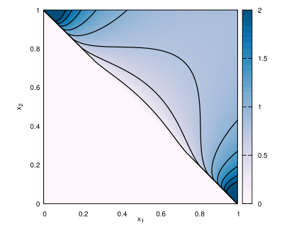
Figure 1: A contour plot that displays our numerical results for the integral $I_{\rm wa}(\theta_{12})$ defined in eq. (183).

The last contribution we need to compute is $\delta\mathcal{F}_{\rm correl}$. Since the $D$-parameter is additive, we can again use the general formula for additive observables in eq. (151). We recast the $D$-parameter, with two soft-collinear emissions, in the form of eq. (150). This gives

$$f_{\rm correl}(\mu,z,\phi,\phi^{(\ell)})=1+\mu^{2}\frac{\sin^{2}(\phi+\phi^{(\ell)})}{\sin^{2}\phi^{(\ell)}}\ \ ,$$ (184)

which is the same for all three legs. This gives

$$\delta\mathcal{F}_{\rm correl}(\lambda)=-\mathcal{F}_{\rm NLL}(\lambda)\sum_{\ell=1}^{3}\frac{\lambda R^{{}^{\prime\prime}}_{\ell,0,\rm NNLL}}{2\beta_{0}\alpha_{s}(Q)}\left(C_{A}\langle\ln f_{\rm correl}\rangle_{C_{A}}+n_{f}\langle\ln f_{\rm correl}\rangle_{n_{f}}\right)\ \ ,$$ (185)

and the various integrals are computed via a Monte Carlo routine

$$\begin{split}\langle\ln f_{\rm correl}\rangle_{C_{A}}&=\frac{1}{2!}\int_{0}^{2\pi}\frac{d\phi^{(\ell)}}{2\pi}\int_{0}^{\infty}\frac{d\mu^{2}}{\mu^{2}(1+\mu^{2})}\int_{0}^{1}dz\int_{0}^{2\pi}\frac{d\phi}{2\pi}(2\mathcal{S}+\mathcal{H}_{g})\ln f_{\rm correl}(\mu,z,\phi,\phi^{(\ell)})=1.8139\ \ ,\\ \langle\ln f_{\rm correl}\rangle_{n_{f}}&=T_{R}\int_{0}^{2\pi}\frac{d\phi^{(\ell)}}{2\pi}\int_{0}^{\infty}\frac{d\mu^{2}}{\mu^{2}(1+\mu^{2})}\int_{0}^{1}dz\int_{0}^{2\pi}\frac{d\phi}{2\pi}\mathcal{H}_{q}\ln f_{\rm correl}(\mu,z,\phi,\phi^{(\ell)})=1.1562\ \ .\end{split}$$ (186)

5 Validation and phenomenology

In this section we validate the analytic results of section 4, match them to fixed order at NLO and finally compare our matched distribution to LEP1 data. We do so in two steps. First, we use the Monte Carlo event generator EVENT2 to check most, but not all, of the pieces in the expansion of the resummation. For the $D$-parameter, EVENT2 provides results at LO, i.e. $\mathcal{O}(\alpha_{s}^{2})$, and thus we will validate all terms in the expansion at $\mathcal{O}(\alpha_{s}^{2})$ up to NNLL. Second, we use NLOJet++ to match the resummation at NLO, i.e. $\mathcal{O}(\alpha_{s}^{3})$. Below we explain our choice of the matching scheme and point out interesting aspects of the resulting phenomenology.

5.1 Partial validation using EVENT2

In this subsection we start with EVENT2 to validate various ingredients in the resummed cumulative distribution of section 4. Given that the Born event is already at $\mathcal{O}(\alpha_{s})$, all the pieces in the expansion of the resummation that starts at $\mathcal{O}(\alpha_{s})$ can then be checked against EVENT2. Table 1 lists these various terms, which contribute at successive logarithmic accuracy. Moreover, the results of EVENT2 are sufficient to validate the geometry dependence in the radiator at NLL, i.e. the $d_{\ell}$-dependent term in eq. (67).

LL	$g_{1}^{(\ell)}(\lambda)$
NLL	$h_{2}^{(\ell)}(\lambda)$
NNLL	$H(\{p\},\alpha_{s}(Q))$   $C^{(1)}_{{\rm hc},\ell}$   $\delta\mathcal{F}_{\rm wa}(\lambda)$   $\delta\mathcal{F}_{\rm rec}(\lambda)$   $\Delta\mathcal{F}_{\rm rec}(\lambda)$

Table 1: The various contributions in the expansion of the resummation that are amenable to validation against EVENT2.

In fig. 2 we expand the resummation of the cumulative cross section and subtract the result from EVENT2. We see indeed that the difference is consistent with zero, and displays an asymptotic behaviour for the entire resummation region.

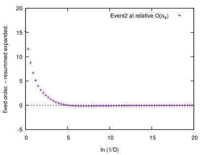
Figure 2: The plot shows the difference between the fixed-order result for the D parameter at LO, i.e. $\mathcal{O}(\alpha_{s}^{2})$, using EVENT2 and the expansion of the resummation from section 4.

Moreover, we can isolate and validate an extra NNLL function using EVENT2 results, i.e. $\delta\mathcal{F}_{\rm correl}(\lambda)$. Indeed, we can not achieve this directly because the fixed-order expansion of $\delta\mathcal{F}_{\rm correl}(\lambda)$ starts at $\mathcal{O}(\alpha_{s}^{2})$. Nevertheless, we can look for an event shape whose behaviour in the presence of correlated emissions is identical to that of the $D$ parameter. We shall call this observable $D_{2-\rm jet}$, and it reads

$$D_{2-\rm jet}=\frac{1}{Q^{2}}\sum_{i<j}\frac{[\hat{n}_{\rm beam}\cdot(\vec{p}_{i}\times\vec{p}_{j})]^{2}}{E_{i}E_{j}}\ \ ,$$ (187)

where $\hat{n}_{\rm beam}$ is a unit vector along the electron beam direction. The design of $D_{2-\rm jet}$ is meant to capture the behaviour of $\delta\mathcal{F}_{\rm correl}(\lambda)$ for the actual $D$-parameter. This observable does not possess a lot of the structure witnessed in three-jet observables, nevertheless, it allows us to check our Monte Carlo implementation for obtaining the results in eq. (186). We have computed the analytic resummation of $D_{2-\rm jet}$, although we do not quote the results here. Fig. 3 shows the result of subtracting the resummed differential distribution from that of EVENT2. Admittedly, the plot in fig. 3 does not exhibit a satisfactory asymptotic behaviour, however, it is quite suggestive. By making use of quadruple precision one should be able to probe sufficiently small values of $D_{2-\rm jet}$.

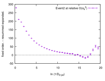
Figure 3: The plot shows the difference between the EVENT2 result for $D_{2-\rm jet}$ at NLO, i.e. $\mathcal{O}(\alpha_{s}^{2})$, and the expansion of the resummation.

Finally, we have also tried to fully validate our resummation of the $D$ parameter, at $\mathcal{O}(\alpha_{s}^{3})$, using NLOJet++. Unfortunately, double precision did not allow us to reach values of $\ln 1/D$ larger than $10-12$, which are not asymptotic enough to provide a reliable validation of our NNLL resummation.

5.2 Matching to fixed order at NLO

In order to provide a suitable cumulative distribution that paves the way for phenomenological studies, one has to match the resummation to fixed order. Matching is required to provide results across all values of the observable. The basic idea is to combine the results of both the resummation and fixed order, while making sure to get rid of contributions that are double counted. There are two generic conditions that the matching procedure must satisfy. First, based on physical grounds the matched total cross section should go to zero as $v\to 0$. Second, the matched distribution, or likewise the total cross section, must reproduce the fixed order at the kinematic endpoint $v\to v_{\rm max}$.

The two most popular matching schemes for $e^{+}e^{-}$ annihilation are the R and log-R schemes Catani:1991kz ; Catani:1992ua . In other contexts, multiplicative matching schemes are used Antonelli:1999kx ; Dasgupta:2001eq . Adopting one over the other is a choice that depends on the problem at hand. In our case, we could not achieve a stable matched distribution using the R and log-R schemes, given that the available data sets for the $D$ parameter forces us to use low values of $y_{\rm cut}$. The problem with both schemes is that, given that the various components of the resummed cross section contain powers of $\ln y_{\rm cut}$, the resummation does not switch off quickly enough and ends up substantially contributing to the tail of the matched distribution. This situation might be expected given that the K-factor NLO/LO is very large, approximately 100 %. This is similar to the case of resuming the distribution in the Higgs transverse momentum $p_{t,H}$ where the K factor is also known to be large Bizon:2017rah . We therefore need to supplement our matching scheme with a factor that effectively damps the resummation at large values of $D$.

Based on the above discussion, we use the multiplicative matching scheme designed in ref. Bizon:2017rah . The goal of that scheme is precisely to suppress the large terms, present in the resummation, which emerge outside the resummation region. This enables us to control the tail of the distribution and achieve a stable matching. In this scheme, matching is performed on the level of the total cross section. Given that NLOJet++ simulates the inclusive cross section, i.e. integrated over Born kinematics with the three-jet selection cut, we have to match on the same level. Explicitly, we have

$$\Sigma_{\mathcal{H}}^{\rm Mat.}(v)=\left(\Sigma_{\mathcal{H}}^{\rm Res.}(v)\right)^{Z}\frac{\Sigma^{\rm{FO.}}_{\mathcal{H}}(v)}{\left(\Sigma_{\mathcal{H}}^{\rm Exp.}(v)\right)^{Z}}\,,$$ (188)

where

$$Z=\left(1-\left(\frac{v}{v_{0}}\right)^{u}\right)^{h}\Theta(v-v_{0})\,,$$ (189)

controls how quickly the logarithms are shut down outside the resummation region. In eq. (188), $\Sigma_{\mathcal{H}}^{\rm Res.}$ is the resummed cross section, $\Sigma^{\rm{FO.}}_{\mathcal{H}}$ is the corresponding fixed-order quantity and $\Sigma_{\mathcal{H}}^{\rm Exp.}$ denotes the expansion of the resummation to NLO. The details of the matching can be found in appendix C and the expanded version of eq. (188) is given in full in eq. (217). The presence of the step function in eq. (189) suggests that the transition region, between the resummation and fixed order, will not be smooth enough. In fact, we verified that even if the step function is removed from the definition of $Z$, the resummation still shuts down smoothly well before reaching the kinematic endpoint $v_{\rm max}$. We carry out the matching using the values $u=1$, $h=3$ and $v_{0}=1/2$.

As is customary in resummed calculations, we need to probe the size of subleading logarithmic terms. This is done using two simultaneous variations. The first introduces a rescaling $x_{V}$ as follows

$$\ln\frac{1}{v}=\ln\frac{x_{V}}{v}-\ln x_{V}\,,\quad x_{V}\equiv X\cdot X_{V}\ \ .$$ (190)

In the above, $X$ is a variable choice to define the resummation scale, i.e. the logarithms being practically resummed, while $X_{V}$ controls the scale variation. We expand the total cross section around $\ln x_{V}/v$ neglecting subleading terms. Furthermore, the resummed logarithm, $\ln x_{V}/v$, must be modified in order to impose that the total cross section is reproduced at the kinematical endpoint $v_{\rm max}$ Dasgupta:2001eq

$$\ln\frac{x_{V}}{v}\to\tilde{L}\equiv\frac{1}{p}\ln\left(\left(\frac{x_{V}}{v}\right)^{p}-\left(\frac{x_{V}}{v_{\rm max}}\right)^{p}+1\right)\ \ ,$$ (191)

where $p$ denotes a positive number that controls how quickly the logarithms are switched off close to the endpoint. The parameter $p$ is free, but is only constrained by the behaviour of the fixed order distribution near the endpoint Dasgupta:2001eq . In our case, we set $p=1$.

Another estimate for the uncertainty in our matched distribution comes from varying the renormalisation scale, $\mu_{R}$, around a central scale that we take to be the centre-of-mass energy of the hard scattering, $Q$. For LEP1 energies, $Q=M_{Z}$ corresponding to $\alpha_{s}(M_{Z})=0.118$ while for FCCee energies, $Q=500\,\rm GeV$ corresponding to $\alpha_{s}(500\,\rm GeV)=0.094$.

We implement two different choices for $X$ in eq. (190). The first is referred to as the $X_{\rm const}$ scheme which corresponds to setting $X=1$ in eq. (190), while the second is the $X_{\rm prod}$ scheme which corresponds to setting

$$X=\frac{3}{2C_{F}+C_{A}}\ln\frac{27\lambda_{1}\lambda_{2}}{2}\ \ ,$$ (192)

which is a function of Born kinematics. Finally, we construct the uncertainty bands by varying $\mu_{R}$ by a factor of two in either direction and $X_{V}$ by a factor of three-halves in either direction.

In figs. 4 and 5 we plot the matched distribution for $Q=M_{Z}$ using the two resummation schemes and for two different values of $y_{\rm cut}$, namely $y_{\rm cut}=0.1$ and $y_{\rm cut}=0.05$. We immediately notice the following features:

• The uncertainty bands are not drastically reduced when increasing the logarithmic accuracy of the resummation, at least when compared to the typical situation with two-jet observables.

• The position of the peak is stable under varying $y_{\rm cut}$.

• For NLL, the uncertainty bands remain almost unchanged with decreasing $y_{\rm cut}$. In contrast, the uncertainty bands for NNLL are noticeably enhanced as we increase $y_{\rm cut}$.

The above features can be traced to the fact that jet selection generates terms that go as $\ln^{2}y_{\rm cut}$, for each power of $\alpha_{s}$ relative to the Born cross section. The largest transverse momentum of soft-collinear emissions, at fixed value of $D$, is of the order of $\sqrt{D}Q$. Our resummation is strictly defined when the largest momentum is much smaller than the largest transverse momentum available, the latter being of the order of $\sqrt{y_{\rm cut}}Q$. Essentially, our resummation is formally correct, as $D\ll 1$, but phenomenologically viable only in the limit $D\ll y_{\rm cut}\ll 1$. Inspection of figs. 4 and 5 shows that the most probable value of $D$, which corresponds to the position of the peak of differential distributions, is of the same order as $y_{\rm cut}$ and that is why we see the features described above. This is also reflected in the sensitivity of the uncertainty bands of the NNLL distribution to the variation of $y_{\rm cut}$ in comparison to NLL. Simply, the NNLL pieces in the cross section, e.g. $\Delta\mathcal{F}_{\rm wa}$, contain extra powers of $\ln y_{\rm cut}$ compared to NLL. These logarithms are large, for $y_{\rm cut}=0.05$-$0.1$, and thus we observe this behaviour of the uncertainty bands.

The situation becomes better at FCC-ee energies, as we see clearly in figs. 6 and 7. Noticeably the position of the peak tends towards smaller values of $D$, and we start approaching the strict resummation regime $D\ll y_{\rm cut}\ll 1$. Simultaneously we see a reduction in the uncertainty by almost $50\%$. To conclude, for this observable, and depending on the value of $y_{\rm cut}$, we expect large subleading corrections that are not under control in any resummation formalism. This calls for a joint resummation of both types of logarithms, the observable and $y_{\rm cut}$, along the line of the presented resummation of both $p_{\rm t,H}$ and the transverse momentum of the leading jet Monni:2019yyr .

Leaving these caveats aside, we note that NNLL corrections generically yield harder $D$-parameter distributions. The effect is larger using the $X_{\rm prod}$ scheme, because the resummed logarithms in the latter scheme are typically larger than the $X_{\rm const}$ scheme. Indeed, this is one of the reasons why the NNLL uncertainty bands get larger when we use the $X_{\rm prod}$ scheme, while their counterparts at NLL remain virtually the same. Note that in the $X_{\rm prod}$ scheme the resummation scale is effectively of the order $\sqrt{y_{\rm cut}}Q$ which is the appropriate upper bound for transverse momenta. Therefore, this scheme automatically captures some of the terms which are enhanced by logarithms of $y_{\rm cut}$.

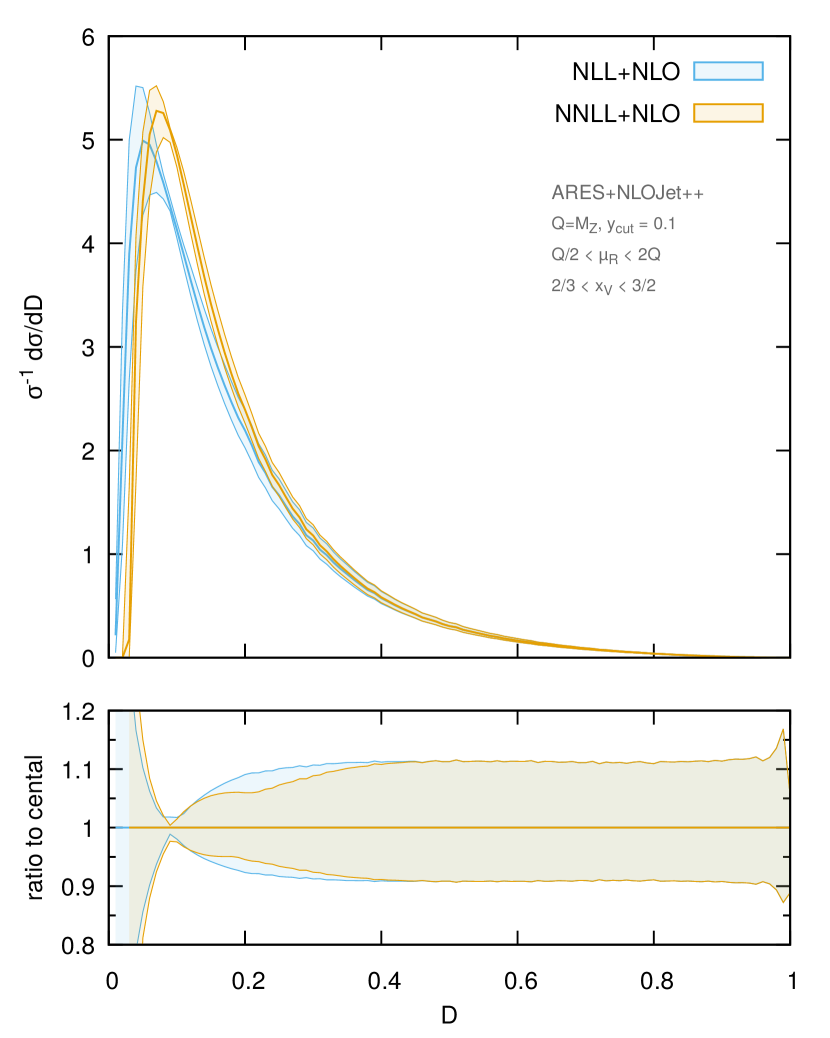
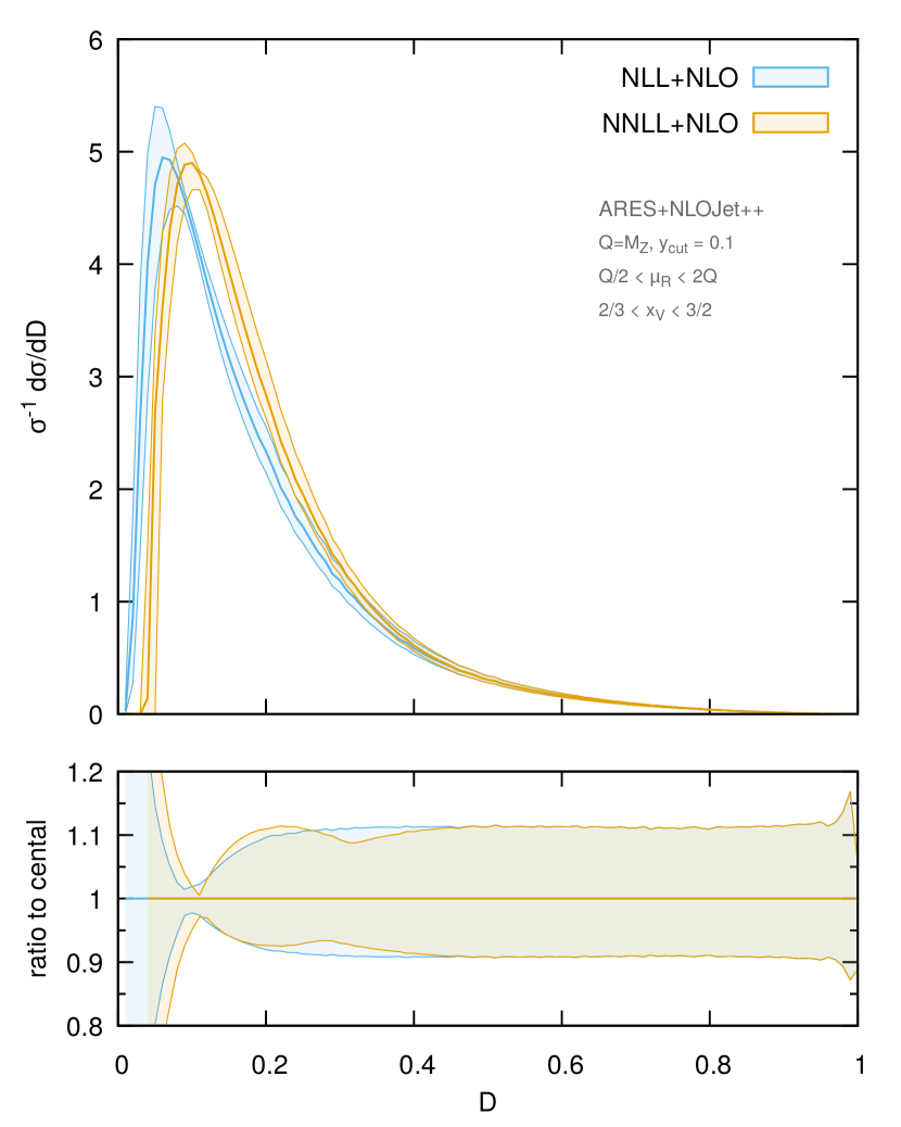
Figure 4: The matched distribution for $y_{\rm cut}=0.1$ and $Q=M_{Z}$. The left plot using the $X_{\rm const}$ scheme and the right using the $X_{\rm prod}$ scheme.

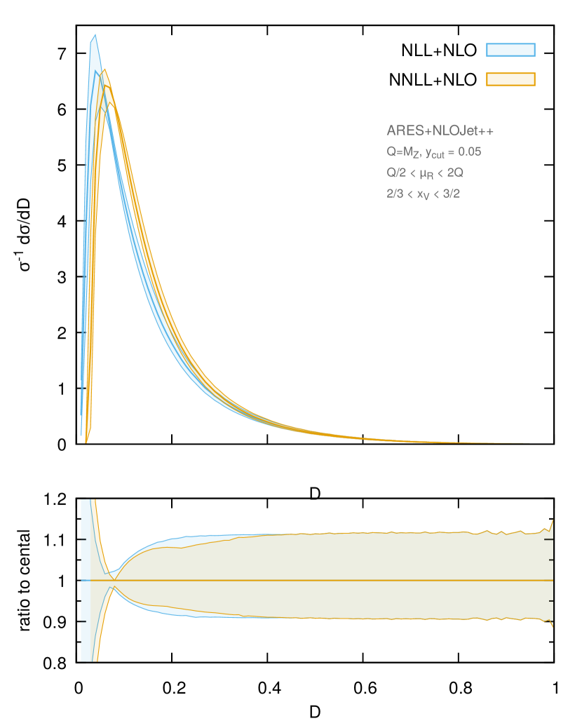
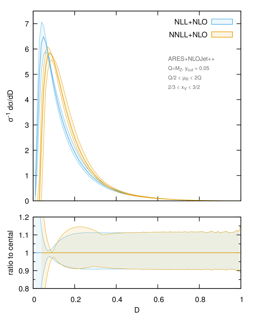
Figure 5: The matched distribution for $y_{\rm cut}=0.05$ and $Q=M_{Z}$. The left plot using the $X_{\rm const}$ scheme and the right using the $X_{\rm prod}$ scheme.

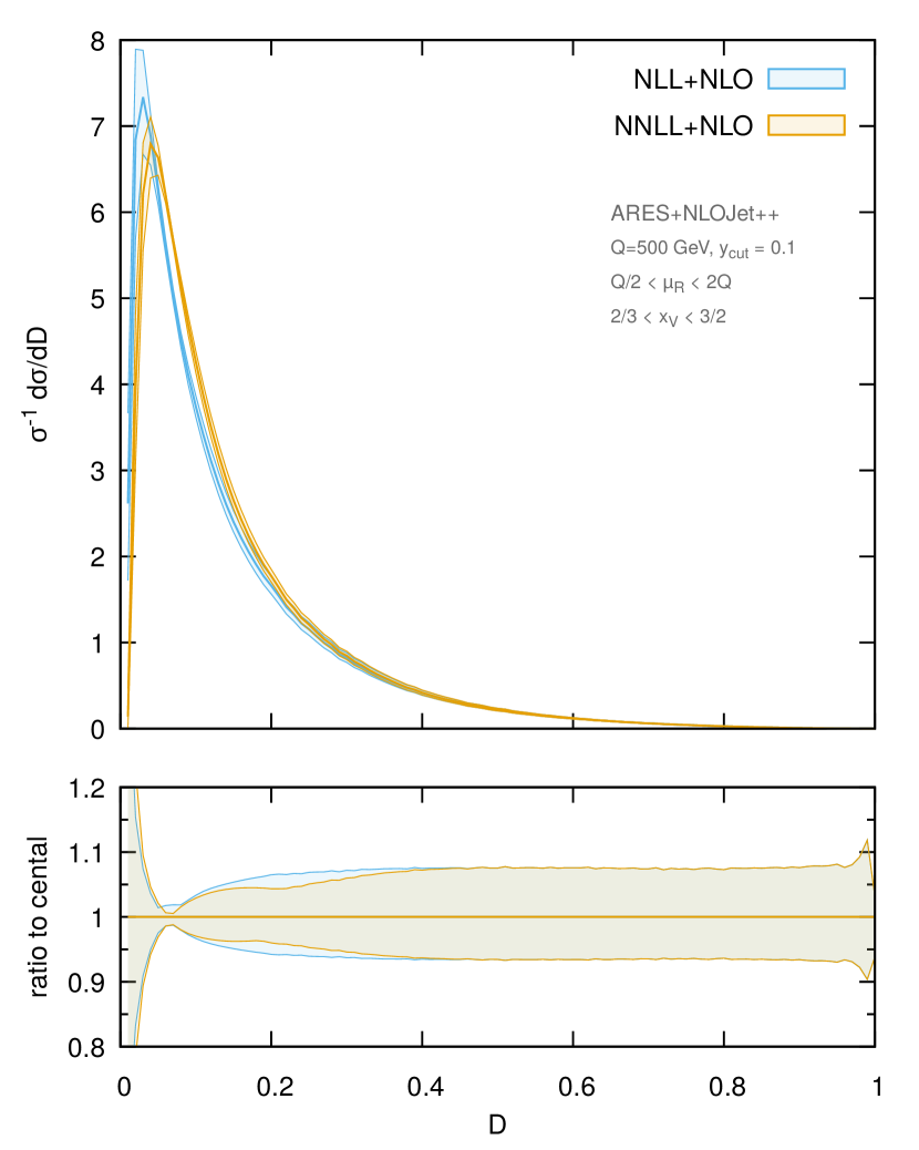
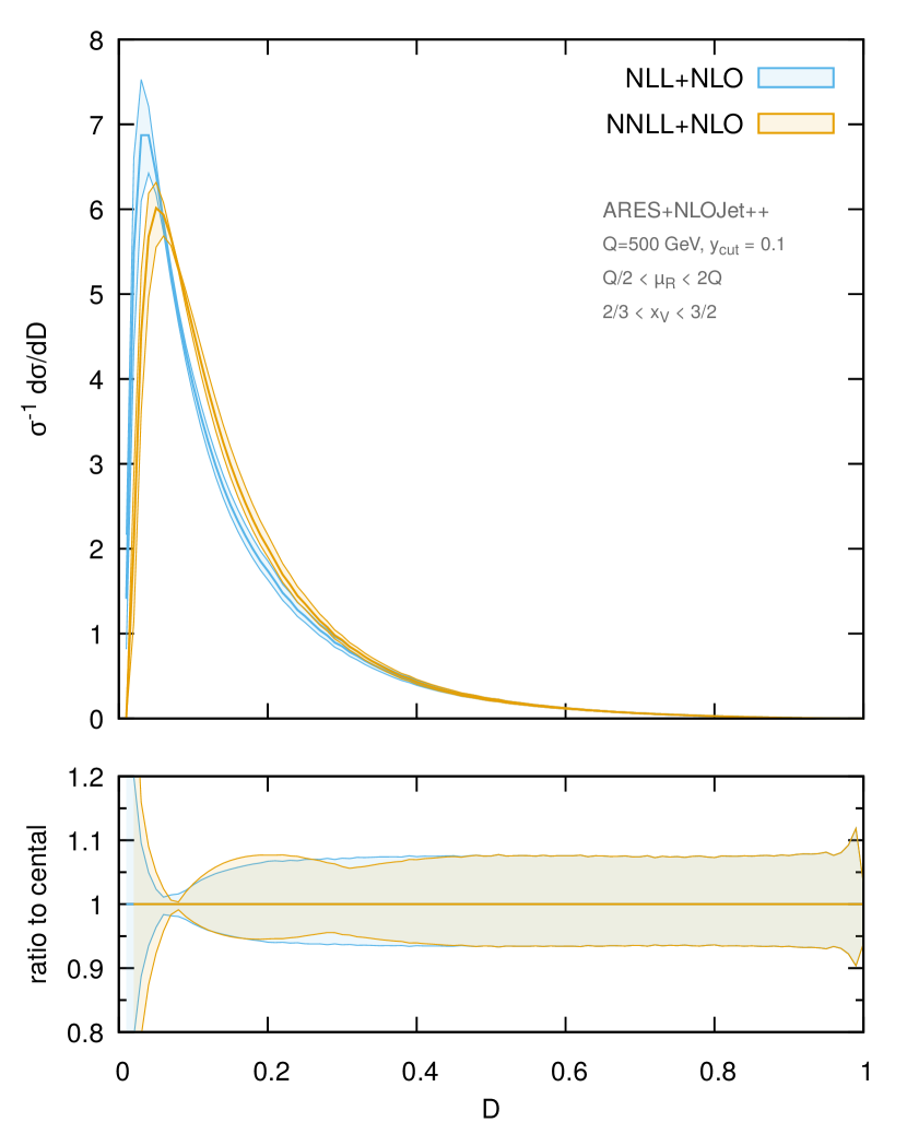
Figure 6: The matched distribution for $y_{\rm cut}=0.1$ and $Q=500\rm GeV$. The left plot using the $X_{\rm const}$ scheme and the right using the $X_{\rm prod}$ scheme.

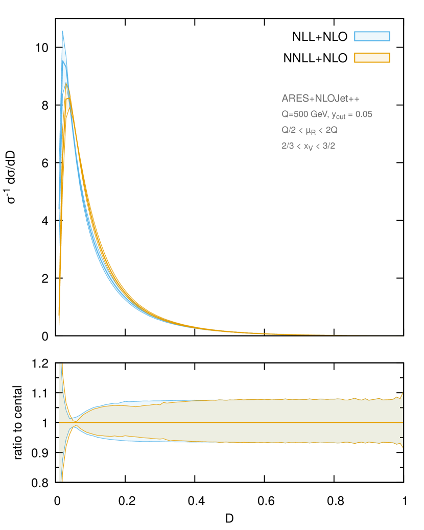
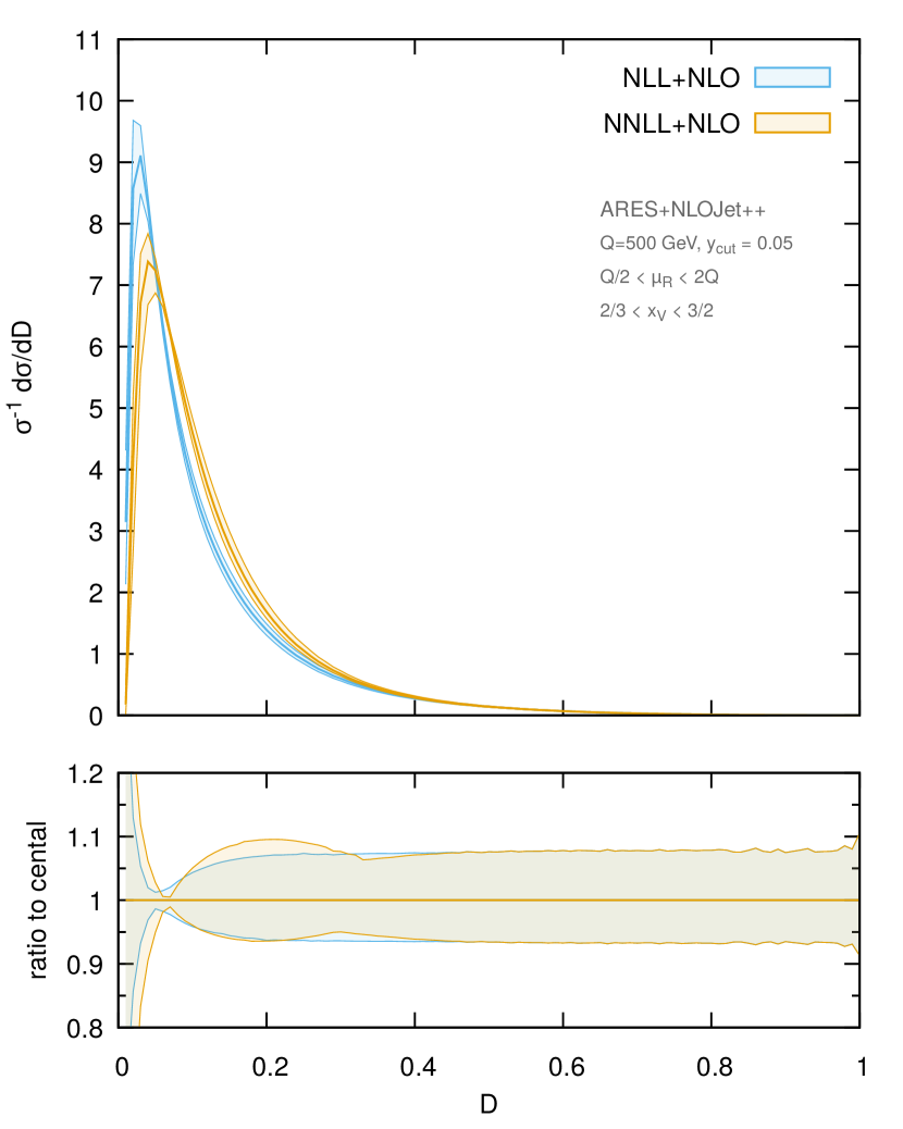
Figure 7: The matched distribution for $y_{\rm cut}=0.05$ and $Q=500\rm GeV$. The left plot using the $X_{\rm const}$ scheme and the right using the $X_{\rm prod}$ scheme.

Last, we compare our predictions to existing LEP1 data alephqcd . In order to do so, we need to supplement our perturbative resummation with some estimate of non-perturbative hadronisation corrections. Before we do this, we need to choose whether to use $X_{\rm const}$ or $X_{\rm prod}$ as our default choice for the resummation scale. We have observed that NNLL distributions obtained with $X_{\rm prod}$ are not very stable with respect to the choice of the matching parameter $v_{0}$, which points to the fact that such a choice brings in numerically large subleading corrections, which we cannot control within our framework. Therefore, we decide to present non-perturbative plots using $X_{\rm const}$ as our resummation scale, and $v_{0}=1/2$. We have checked that using other values of $v_{0}$ does not change considerably our findings. We include hadronisation corrections in the dispersive approach of ref. Dokshitzer:1995qm , where leading hadronisation corrections result in a shift of the corresponding perturbative distributions. In our case, we use the non-perturbative shift computed in ref. Banfi:2001pb , and define

$$\Sigma_{\mathcal{H}}^{\rm NP}(D)=\frac{1}{\sigma_{\mathcal{H}}}\int d\Phi_{3}\frac{d\sigma_{3}}{d\Phi_{3}}\Sigma_{\mathcal{B}}\left(\{p_{1},p_{2},p_{3}\},D-Z_{\rm NP}\,\delta D\left(\{p_{1},p_{2},p_{3}\}\right)\right)\,\mathcal{H}(p_{1},p_{2},p_{3})\,,$$ (193)

where

$$\delta D(\{p_{1},p_{2},p_{3}\})=\frac{a_{\rm NP}}{Q}27\lambda_{1}\lambda_{2}\sum_{(ij)}C_{(ij)}\,g_{ij}\left(\theta_{ij}\right)\,.$$ (194)

In the above equation, the geometry dependent functions $g_{ij}$ are the ones of ref. Banfi:2001pb , which we rewrite using our own notation and conventions as follows:

$$g_{ij}(\theta_{ij})=\sin\frac{\theta_{ij}}{2}\int_{0}^{2\pi}\frac{d\phi}{2\pi}\int_{-\infty}^{\infty}d\eta\frac{\sin^{2}\phi}{\cosh\eta+\cos(\theta_{ij}/2)\cos\phi}\,.$$ (195)

The non-perturbative parameter $a_{\rm NP}$ is given by

$$a_{\rm NP}=\frac{4\mu_{I}}{\pi^{2}}\mathcal{M}\left(\alpha_{0}(\mu_{I})-\alpha_{s}(Q)-2\beta_{0}\alpha^{2}_{s}(Q)\left(\ln\frac{Q}{\mu_{I}}+\frac{K^{(1)}}{4\pi\beta_{0}}+1\right)\right)\,,$$ (196)

where

$$\alpha_{0}(\mu_{I})=\int_{0}^{\mu_{I}}\frac{dk}{\mu_{I}}\alpha_{s}(k)\,,$$ (197)

and $\alpha_{s}(k)$ is the dispersive coupling defined in ref. Dokshitzer:1995qm . As in previous non-perturbative studies, we set $\mu_{I}=2\,$GeV. In eq. (193), we have also introduced the factor

$$Z_{\rm NP}=1-\left(\frac{D}{D_{\rm max}}\right)^{q}\,,$$ (198)

that ensures that the shift vanishes at the endpoint of the distribution. Also, to ensure that the distribution vanishes at its endpoint, we replace $\tilde{L}$ defined in eq. (191) with

$$\tilde{L}_{\rm NP}\equiv\frac{1}{p}\ln\left(\left(\frac{x_{D}}{D-\delta D}\right)^{p}-\left(\frac{x_{D}}{D_{\rm max}-\delta D}\right)^{p}+1\right)\,.$$ (199)

Specifically, we have set $q=2$ and $p=1$. Last, in order to produce matched non-perturbative distributions, we compute $\delta D_{\mathcal{H}}$ defined by

$$\Sigma_{\cal H}(D-\delta D_{\mathcal{H}})=\Sigma_{\mathcal{H}}^{\rm NP}(D)\,,$$ (200)

and define our matched non-perturbative distribution as $\Sigma^{\rm Mat.}_{\cal H}(D-\delta D_{\mathcal{H}})$.

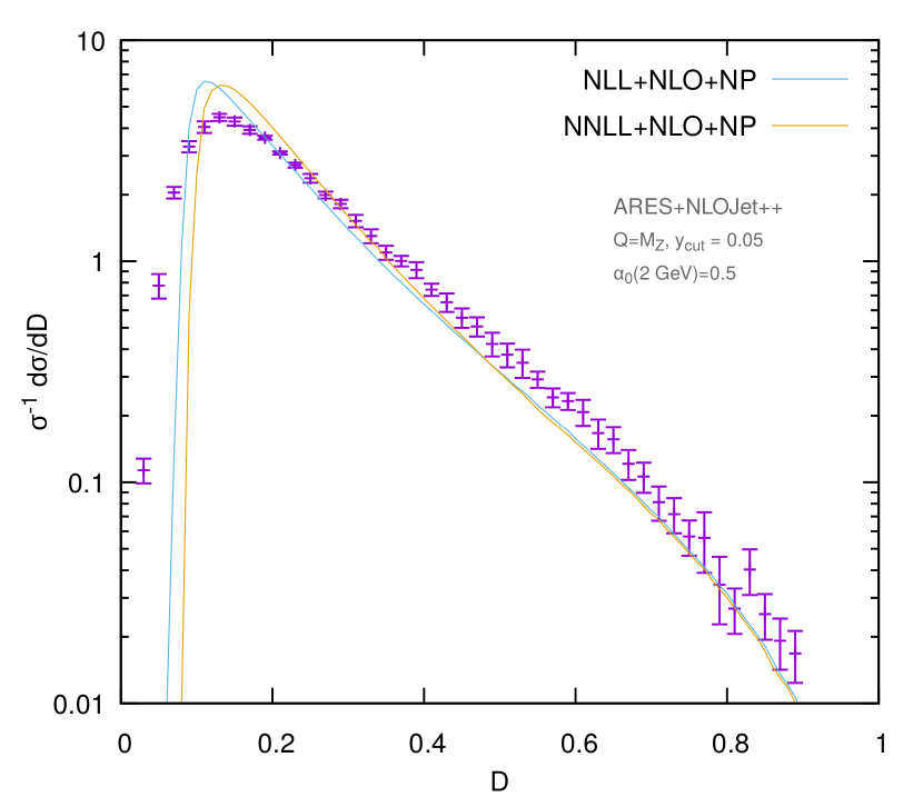
Figure 8: The matched distribution, including the non-perturbative corrections, is compared to data from LEP1 for the two values of $y_{\rm cut}$ we adopt in this article.

In Fig. 8 we produce plots for non-perturbative matched distributions, with central scales, corresponding to NLL and NNLL accuracy. The non-perturbative shift corresponds to a value of $\alpha_{0}(2\,\mathrm{GeV})$ that give us a good agreement with data, and is within the range favoured by existing fits to event-shape data Salam:2001bd . We see that NNLL resummation has a shape that resembles data more closely than NLL resummation, whilst favouring a similar value of $\alpha_{0}$, namely $\alpha_{0}=0.5$. This trend persists irrespective of the value of $y_{\rm cut}$. This value of $\alpha_{0}$ is similar to the central value of a fit obtained with the NNLL thrust distribution Gehrmann:2012sc . Finally, increasing the value of $v_{0}$ up to $D_{\max}$ does not change the distributions close to the peak, but gives a better agreement with data in the tails.

6 Conclusions

This article presents a general method to compute the NNLL resummation of rIRC safe observables for processes characterised by the presence of three hard emitters. The method is a generalisation of the ARES approach to NNLL resummations, and paves the way to a general NNLL resummation with an arbitrary number of hard emitters. Although we concentrate on three-jet events in $e^{+}e^{-}$ annihilation, our treatment of NNLL contributions induced by final-state radiation is completely general.

Similar to the two-jet case, we are able to combine unresolved real radiation and virtual corrections to the Born process into an analytically computable NNLL radiator. The remaining corrections are all induced by real radiation, and can be computed for a general observable using suitable Monte-Carlo procedures.

Two new functions appear in the three-jet case. First, a new NNLL correction of soft wide-angle origin appears, due to the fact that now we have three-hard emitters with non-trivial colour correlations. Second, since we have a hard gluon initiating a three-jet event, we need to take into account non-trivial spin correlations in hard-collinear splittings. These are embedded in a new NNLL correction that adds to those of hard-collinear origin.

As an example, we have applied our method to the $D$-parameter. Since this is an additive observable, we are able to compute most NNLL functions analytically, with a couple of integrals to be computed numerically. Then, we have performed phenomenological studies by matching our resummation to exact fixed-order and presenting predictions for LEP1 and future colliders. Both validation of resummation and phenomenology is tricky for three-jet observables. First, while it is possible to easily check NLL contributions against exact fixed-order, it is impossible to check NNLL ones without resorting to quadruple precision. With the aid of a fake two-jet observable that resembles the $D$-parameter, we have been able to check some NNLL contributions using the NLO code EVENT2. For what concerns the actual phenomenology, current cuts to select three-jet events give rise to large subleading effects at LEP1 energies. The situation is a bit better at FCC-ee. Nevertheless, we envisage that, to improve phenomenological studies of the $D$-parameter, one should attempt a joint resummation of logarithms of the $D$-parameter and of the variable determining the three-jet selection, with a similar procedure to that for angularites, or for the transverse momentum of a colour singlet and an accompanying leading jet.

A comparison with LEP1 data requires the inclusion of non-perturbative hadronisation corrections. We have added to our NNLL resummation the leading hadronisation corrections evaluated in the dispersive model. In general, the NNLL distribution has a shape that is similar to data, so hadronisation corrections are compatible with a rigid shift of perturbative distributions. We find that the value of the non-perturbative parameter $\alpha_{0}$ determining the size of hadronisation corrections is comparable to the one obtained with NLL distributions. It might be very interesting at this stage to perform a comprehensive simultaneous fit of $\alpha_{s}$ and $\alpha_{0}$ using NNLL resummations for different event shapes.

In conclusion, our study sets the main building blocks for a general NNLL resummation of rIRC safe final-state observables with an arbitrary number of hard emitting legs. The only missing ingredient is a general treatment of both initial-state radiation and soft wide-angle corrections for a system with more than three hard emitting legs. Despite the technical difficulties, the philosophy of our method stays unchanged. In particular, ARES does not depend on the specific factorisation properties of an observable, and gives promise to achieve a fully general solution to the problem of NNLL resummation in the near future.

Appendix A Correlated two-parton emission

The double-emission function $\mathcal{A}^{2}$ in eq. (118) reads

$$\mathcal{A}^{2}=C_{A}(2\mathcal{S}+\mathcal{H}_{g})+n_{f}\mathcal{H}_{q}\ \ ,$$ (201)

where

$$2\mathcal{S} =\frac{1}{z(1-z)}\left[\frac{1-(1-z)\mu^{2}/z}{u_{a}^{2}}+\frac{1-z\mu^{2}/(1-z)}{u_{b}^{2}}\right]$$ (202a)

$$\mathcal{H}_{g} =-4+\frac{z(1-z)}{1+\mu^{2}}\left(2\cos\phi+\frac{(1-2z)\mu}{\sqrt{z(1-z)}}\right)^{2}$$

$$+\frac{1}{2(1-z)}\left[1-\frac{1-(1-z)\mu^{2}/z}{u_{a}^{2}}\right]+\frac{1}{2z}\left[1-\frac{1-z\mu^{2}/(1-z)}{u_{b}^{2}}\right]$$ (202b)

$$\mathcal{H}_{q} =1-\frac{z(1-z)}{1+\mu^{2}}\left(2\cos\phi+\frac{(1-2z)\mu}{\sqrt{z(1-z)}}\right)^{2}\,.$$ (202c)

In the above equations, we also defined the following quantities

$$u_{a}^{2}=1+2\sqrt{\frac{1-z}{z}}\mu\cos\phi+\frac{1-z}{z}\mu^{2}\,,\qquad u_{b}^{2}=1-2\sqrt{\frac{z}{1-z}}\mu\cos\phi+\frac{z}{1-z}\mu^{2}\,.$$ (203)

Note, in particular, that the quark function $\mathcal{H}_{q}$ is defined with a factor of 2 to compensate for the symmetry $1/2!$ in the phase space. Now it should be useful to demonstrate explicitly the variables transformations we implemented in the matrix element. Indeed, the form of eq. (118) does not depend on the specific dipole to which the correlated soft pair belongs to. Nevertheless, we introduce the Sudakov decomposition of each momentum in a certain dipole

$$k_{a}^{(ij)} =z_{a}^{(i)}\,p_{i}+z_{a}^{(j)}\,p_{j}+\kappa_{a}^{(ij)}\cos\phi_{a}^{(ij)}\,n^{(ij)}_{\rm in}+\kappa^{(ij)}\sin\phi_{a}^{(ij)}\,n^{(ij)}_{\rm out}\ \ ,$$ (204)

$$k_{b}^{(ij)} =z_{b}^{(i)}\,p_{i}+z_{b}^{(j)}\,p_{j}+\kappa_{b}^{(ij)}\cos\phi_{b}^{(ij)}\,n^{(ij)}_{\rm in}+\kappa_{b}^{(ij)}\sin\phi_{b}^{(ij)}\,n^{(ij)}_{\rm out}\ \ .$$ (205)

Our task is to express the emission’s Sudakov variables in terms of the Sudakov variables of the pseudo-parent momentum, defined as $k=k_{a}+k_{b}$. Now in the Euclidean two-dimensional plane spanned by the pair $(\vec{n}^{(ij)}_{\rm in},\vec{n}^{(ij)}_{\rm out})$, we define two vectors

$$\vec{k}^{(ij)}_{a}\equiv\kappa_{a}^{(ij)}\cos\phi_{a}^{(ij)}\,\vec{n}^{(ij)}_{\rm in}+\kappa^{(ij)}\sin\phi_{a}^{(ij)}\,\vec{n}^{(ij)}_{\rm out},\quad\vec{k}^{(ij)}_{b}\equiv\kappa_{b}^{(ij)}\cos\phi_{b}^{(ij)}\,\vec{n}^{(ij)}_{\rm in}+\kappa_{b}^{(ij)}\sin\phi_{b}^{(ij)}\,\vec{n}^{(ij)}_{\rm out}\ \ ,$$ (206)

which play the role of transverse momenta and allows us to directly utilise the results of ref. Banfi:2018mcq . We henceforth list the variables appearing in eq. (118)

$$\frac{z}{1-z}=\frac{z_{a}^{(i)}}{z_{b}^{(i)}},\quad\vec{q}^{~{}(ij)}=z\vec{k}^{(ij)}_{a}+(1-z)\vec{k}^{(ij)}_{b},\quad\mu^{2}=\frac{(k_{a}+k_{b})^{2}}{(\vec{k}^{(ij)}_{a}+\vec{k}^{(ij)}_{b})^{2}},\quad\cos\phi=\frac{\vec{q}^{~{}(ij)}\cdot\vec{k}^{(ij)}}{(\vec{k}^{(ij)})^{2}(\vec{q}^{~{}(ij)})^{2}}\ \ .$$ (207)

Appendix B Three-parton kinematics

We consider three momenta $p_{1},p_{2},p_{3}$, with $p_{1}+p_{2}+p_{3}=q=(Q,0,0,0)$. Using a flavour-based labelling, $p_{1}$ is a quark, $p_{2}$ an antiquark and $p_{3}$ a gluon. We define the dimensionless variables $x_{i}=2(p_{i}q)/Q^{2}<1$, satisfying $x_{1}+x_{2}+x_{3}=2$. In terms of these variables,

$$E_{i}=x_{i}\frac{Q}{2}\,,\qquad 2(p_{i}p_{j})=(x_{i}+x_{j}-1)Q^{2}\,.$$ (208)

This makes it possible to write the angles between pairs of momenta in terms of the $x_{i}$’s as follows

$$\sin^{2}\frac{\theta_{ij}}{2}=\frac{x_{i}+x_{j}-1}{x_{i}\,x_{j}}\,.$$ (209)

The three-parton cross section, differential in $x_{1}$ and $x_{2}$, in four dimensions reads

$$\frac{d\sigma}{dx_{1}dx_{2}}=\sigma_{0}C_{F}\frac{\alpha_{s}}{2\pi}\frac{x_{1}^{2}+x_{2}^{2}}{(1\!-\!x_{1})(1\!-\!x_{2})}$$ (210)

with $\sigma_{0}$ the Born cross section for producing a quark-antiquark pair in $e^{+}e^{-}$ annihilation.

To obtain the Born three-jet cross section $\sigma_{0}(y_{\rm cut})$ with the Durham algorithm Catani:1991hj we need to integrate the differential cross section in eq. (210) with the constraint $y_{3}(p_{1},p_{2},p_{3})=\min\{y_{12},y_{13},y_{23}\}>y_{\rm cut}$, where $y_{ij}$ is the “distance” between pairs of partons defined by

$$y_{ij}\equiv 2\frac{\min\{E_{i}^{2},E_{j}^{2}\}}{Q^{2}}(1-\cos\theta_{ij})=\min\left\{\frac{x_{i}}{x_{j}},\frac{x_{j}}{x_{i}}\right\}(x_{i}+x_{j}-1)\,.$$ (211)

The Durham algorithm defines a six-sided region in the $(x_{1},x_{2})$ plane, as shown in Fig. 9 for the three different values of $y_{\rm cut}$ we consider here.

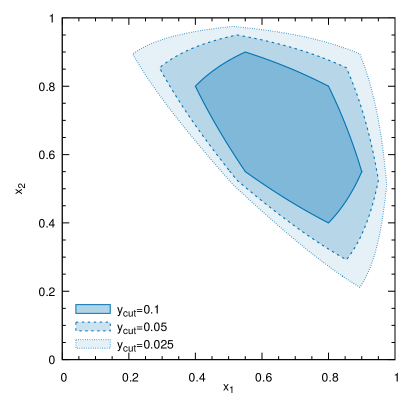
Figure 9: The Durham algorithm three-jet region for three different values of $y_{\rm cut}$.

The corresponding Born cross section $\sigma^{(0)}_{\cal H}$ is

$$\begin{split}\sigma^{(0)}_{\cal H}&=\sigma_{0}C_{F}\frac{\alpha_{s}}{2\pi}\int_{0}^{1}dx_{1}\,\int_{0}^{1}dx_{2}\frac{x_{1}^{2}+x_{2}^{2}}{(1\!-\!x_{1})(1\!-\!x_{2})}\,\Theta(x_{1}+x_{2}\!-\!1)\,\Theta\left(\min\{y_{12},y_{13},y_{23}\}\!-\!y_{\rm cut}\right)\,.\end{split}$$ (212)

This cross section can be computed analytically. Its expression, not particularly illuminating, can be found in Brown:1991hx .

Appendix C Full matching formulae

In our matching formulae $\Sigma^{\rm Mat.}_{\mathcal{H}}(v)$ we normalise all of the distributions to the total cross section $\sigma_{\mathcal{H}}$. However this is not what is provided by NLOjet++, instead it provides the un-normalised differential distribution for the $D$-parameter. We can transform the output of NLOjet++ into our conventions as follows. First we compute the un-normalised, barred, total cross section

$$\bar{\Sigma}^{(i)}_{\rm NLOJet}=-\int_{v}^{v_{\rm max}}dv^{\prime}\frac{d\Sigma^{(i)}_{\rm NLOJet}(v^{\prime})}{dv^{\prime}}\,,$$ (213)

where $i$ refers to the power of $\alpha_{s}$ in perturbation theory. To transform this result into our conventions we perform the following manipulations

$$\begin{split}\bar{\Sigma}^{(1)}_{\rm FO.}(v)&=\frac{\bar{\Sigma}^{(1)}_{\rm NLOJet}(v)}{\sigma^{(0)}_{\mathcal{H}}}\,,\\ \bar{\Sigma}^{(2)}_{\rm FO.}(v)&=\frac{\bar{\Sigma}^{(2)}_{\rm NLOJet}(v)}{\sigma^{(0)}_{\mathcal{H}}}-\frac{\sigma^{(1)}_{\mathcal{H}}}{\sigma^{(0)}_{\mathcal{H}}}\bar{\Sigma}^{(1)}_{\rm FO.}(v)\,.\end{split}$$ (214)

In terms of the barred variables we have

$$\begin{split}\Sigma_{\rm FO.}(v)&=\sum_{i=0}^{2}\Sigma^{(i)}_{\rm FO.}(v)\\ &=1+\sum_{i=1}^{2}\bar{\Sigma}^{(i)}_{\rm FO.}(v)\,,\end{split}$$ (215)

and analogously for the expansion of the resummation

$$\Sigma_{\rm Exp.}(v)=\sum_{i=0}^{2}\Sigma^{(i)}_{\rm Exp.}(v)\,.$$ (216)

Finally we can present the explicit form of our matched distribution in eq. (188)

$$\begin{split}\Sigma_{\rm Mat.}(v)&=\left(\Sigma_{\rm Res.}(v)\right)^{Z}\left[1+\bar{\Sigma}^{(1)}_{\rm FO.}(v)-Z\Sigma^{(1)}_{\rm Exp.}(v)+\right.\\ &\left.+\bar{\Sigma}^{(2)}_{\rm FO.}(v)-Z\Sigma^{(2)}_{\rm Exp.}(v)-Z\Sigma^{(1)}_{\rm Exp.}(v)\left(\Sigma^{(1)}_{\rm FO.}(v)-\frac{Z+1}{2}\Sigma^{(1)}_{\rm Exp.}(v)\right)\right]\,.\end{split}$$ (217)

References

- (1) Particle Data Group collaboration, Review of Particle Physics, Chin. Phys. C40 (2016) 100001.
- (2) M. Dasgupta and G. P. Salam, Resummation of nonglobal QCD observables, Phys. Lett. B512 (2001) 323 [hep-ph/0104277].
- (3) M. Dasgupta and G. P. Salam, Accounting for coherence in interjet E(t) flow: A Case study, JHEP 03 (2002) 017 [hep-ph/0203009].
- (4) A. Banfi, G. Marchesini and G. Smye, Away from jet energy flow, JHEP 08 (2002) 006 [hep-ph/0206076].
- (5) R. K. Ellis, D. A. Ross and A. E. Terrano, The Perturbative Calculation of Jet Structure in e+ e- Annihilation, Nucl. Phys. B178 (1981) 421.
- (6) A. Gehrmann-De Ridder, T. Gehrmann, E. W. N. Glover and G. Heinrich, NNLO corrections to event shapes in e+ e- annihilation, JHEP 12 (2007) 094 [0711.4711].
- (7) A. Gehrmann-De Ridder, T. Gehrmann, E. W. N. Glover and G. Heinrich, Jet rates in electron-positron annihilation at O(alpha(s)**3) in QCD, Phys. Rev. Lett. 100 (2008) 172001 [0802.0813].
- (8) S. Weinzierl, NNLO corrections to 3-jet observables in electron-positron annihilation, Phys. Rev. Lett. 101 (2008) 162001 [0807.3241].
- (9) S. Weinzierl, Event shapes and jet rates in electron-positron annihilation at NNLO, JHEP 06 (2009) 041 [0904.1077].
- (10) J. C. Collins, D. E. Soper and G. F. Sterman, Transverse Momentum Distribution in Drell-Yan Pair and W and Z Boson Production, Nucl. Phys. B250 (1985) 199.
- (11) S. Catani, G. Turnock and B. R. Webber, Heavy jet mass distribution in e+ e- annihilation, Phys. Lett. B272 (1991) 368.
- (12) S. Catani, G. Turnock, B. R. Webber and L. Trentadue, Thrust distribution in e+ e- annihilation, Phys. Lett. B263 (1991) 491.
- (13) S. Catani, L. Trentadue, G. Turnock and B. R. Webber, Resummation of large logarithms in e+ e- event shape distributions, Nucl. Phys. B407 (1993) 3.
- (14) Y. L. Dokshitzer, A. Lucenti, G. Marchesini and G. P. Salam, On the QCD analysis of jet broadening, JHEP 01 (1998) 011 [hep-ph/9801324].
- (15) R. Bonciani, S. Catani, M. L. Mangano and P. Nason, Sudakov resummation of multiparton QCD cross-sections, Phys. Lett. B575 (2003) 268 [hep-ph/0307035].
- (16) A. Banfi, G. P. Salam and G. Zanderighi, Semi-numerical resummation of event shapes, JHEP 01 (2002) 018 [hep-ph/0112156].
- (17) A. Banfi, G. P. Salam and G. Zanderighi, Generalized resummation of QCD final state observables, Phys. Lett. B584 (2004) 298 [hep-ph/0304148].
- (18) A. Banfi, G. P. Salam and G. Zanderighi, Principles of general final-state resummation and automated implementation, JHEP 03 (2005) 073 [hep-ph/0407286].
- (19) A. Banfi, G. P. Salam and G. Zanderighi, Resummed event shapes at hadron - hadron colliders, JHEP 08 (2004) 062 [hep-ph/0407287].
- (20) A. Banfi, G. P. Salam and G. Zanderighi, Phenomenology of event shapes at hadron colliders, JHEP 06 (2010) 038 [1001.4082].
- (21) M. Dasgupta, F. A. Dreyer, K. Hamilton, P. F. Monni and G. P. Salam, Logarithmic accuracy of parton showers: a fixed-order study, JHEP 09 (2018) 033 [1805.09327].
- (22) Y. L. Dokshitzer, G. Marchesini and G. P. Salam, Revisiting nonperturbative effects in the jet broadenings, Eur. Phys. J.direct 1 (1999) 3 [hep-ph/9812487].
- (23) G. P. Salam and D. Wicke, Hadron masses and power corrections to event shapes, JHEP 05 (2001) 061 [hep-ph/0102343].
- (24) T. Gehrmann, G. Luisoni and P. F. Monni, Power corrections in the dispersive model for a determination of the strong coupling constant from the thrust distribution, Eur. Phys. J. C73 (2013) 2265 [1210.6945].
- (25) R. Abbate, M. Fickinger, A. H. Hoang, V. Mateu and I. W. Stewart, Thrust at N3LL with Power Corrections and a Precision Global Fit for , Phys. Rev. D83 (2011) 074021 [1006.3080].
- (26) A. H. Hoang, D. W. Kolodrubetz, V. Mateu and I. W. Stewart, -parameter distribution at N3LL? including power corrections, Phys. Rev. D91 (2015) 094017 [1411.6633].
- (27) A. H. Hoang, D. W. Kolodrubetz, V. Mateu and I. W. Stewart, Precise determination of from the -parameter distribution, Phys. Rev. D91 (2015) 094018 [1501.04111].
- (28) T. Becher and M. D. Schwartz, A precise determination of from LEP thrust data using effective field theory, JHEP 07 (2008) 034 [0803.0342].
- (29) P. F. Monni, T. Gehrmann and G. Luisoni, Two-Loop Soft Corrections and Resummation of the Thrust Distribution in the Dijet Region, JHEP 08 (2011) 010 [1105.4560].
- (30) Y.-T. Chien and M. D. Schwartz, Resummation of heavy jet mass and comparison to LEP data, JHEP 08 (2010) 058 [1005.1644].
- (31) T. Becher and M. Neubert, Factorization and NNLL Resummation for Higgs Production with a Jet Veto, JHEP 07 (2012) 108 [1205.3806].
- (32) D. de Florian and M. Grazzini, The Back-to-back region in e+ e- energy-energy correlation, Nucl. Phys. B704 (2005) 387 [hep-ph/0407241].
- (33) Z. Tulipánt, A. Kardos and G. Somogyi, Energyenergy correlation in electronpositron annihilation at NNLL + NNLO accuracy, Eur. Phys. J. C77 (2017) 749 [1708.04093].
- (34) I. Moult and H. X. Zhu, Simplicity from Recoil: The Three-Loop Soft Function and Factorization for the Energy-Energy Correlation, JHEP 08 (2018) 160 [1801.02627].
- (35) C. Frye, A. J. Larkoski, M. D. Schwartz and K. Yan, Factorization for groomed jet substructure beyond the next-to-leading logarithm, JHEP 07 (2016) 064 [1603.09338].
- (36) M. Procura, W. J. Waalewijn and L. Zeune, Joint resummation of two angularities at next-to-next-to-leading logarithmic order, JHEP 10 (2018) 098 [1806.10622].
- (37) G. Bell, A. Hornig, C. Lee and J. Talbert, angularity distributions at NNLL′ accuracy, JHEP 01 (2019) 147 [1808.07867].
- (38) D. Kang, C. Lee and I. W. Stewart, Using 1-Jettiness to Measure 2 Jets in DIS 3 Ways, Phys. Rev. D88 (2013) 054004 [1303.6952].
- (39) Z.-B. Kang, X. Liu, S. Mantry and J.-W. Qiu, Probing nuclear dynamics in jet production with a global event shape, Phys. Rev. D88 (2013) 074020 [1303.3063].
- (40) Z.-B. Kang, X. Liu and S. Mantry, 1-jettiness DIS event shape: NNLL+NLO results, Phys. Rev. D90 (2014) 014041 [1312.0301].
- (41) G. Bozzi, S. Catani, D. de Florian and M. Grazzini, Transverse-momentum resummation and the spectrum of the Higgs boson at the LHC, Nucl. Phys. B737 (2006) 73 [hep-ph/0508068].
- (42) T. Becher and M. Neubert, Drell-Yan Production at Small , Transverse Parton Distributions and the Collinear Anomaly, Eur. Phys. J. C71 (2011) 1665 [1007.4005].
- (43) A. Banfi, M. Dasgupta and S. Marzani, QCD predictions for new variables to study dilepton transverse momenta at hadron colliders, Phys. Lett. B701 (2011) 75 [1102.3594].
- (44) I. W. Stewart, F. J. Tackmann and W. J. Waalewijn, The Beam Thrust Cross Section for Drell-Yan at NNLL Order, Phys. Rev. Lett. 106 (2011) 032001 [1005.4060].
- (45) C. F. Berger, C. Marcantonini, I. W. Stewart, F. J. Tackmann and W. J. Waalewijn, Higgs Production with a Central Jet Veto at NNLL+NNLO, JHEP 04 (2011) 092 [1012.4480].
- (46) T. Becher, X. Garcia i Tormo and J. Piclum, Next-to-next-to-leading logarithmic resummation for transverse thrust, Phys. Rev. D93 (2016) 054038 [1512.00022].
- (47) T. Becher, M. Neubert and L. Rothen, Factorization and +NNLO predictions for the Higgs cross section with a jet veto, JHEP 10 (2013) 125 [1307.0025].
- (48) A. Banfi, P. F. Monni, G. P. Salam and G. Zanderighi, Higgs and Z-boson production with a jet veto, Phys. Rev. Lett. 109 (2012) 202001 [1206.4998].
- (49) I. W. Stewart, F. J. Tackmann, J. R. Walsh and S. Zuberi, Jet resummation in Higgs production at , Phys. Rev. D89 (2014) 054001 [1307.1808].
- (50) S. Catani, M. Grazzini and A. Torre, Transverse-momentum resummation for heavy-quark hadroproduction, Nucl. Phys. B890 (2014) 518 [1408.4564].
- (51) H. X. Zhu, C. S. Li, H. T. Li, D. Y. Shao and L. L. Yang, Transverse-momentum resummation for top-quark pairs at hadron colliders, Phys. Rev. Lett. 110 (2013) 082001 [1208.5774].
- (52) I. W. Stewart, F. J. Tackmann and W. J. Waalewijn, N-Jettiness: An Inclusive Event Shape to Veto Jets, Phys. Rev. Lett. 105 (2010) 092002 [1004.2489].
- (53) T. T. Jouttenus, I. W. Stewart, F. J. Tackmann and W. J. Waalewijn, The Soft Function for Exclusive N-Jet Production at Hadron Colliders, Phys. Rev. D83 (2011) 114030 [1102.4344].
- (54) W. Bizon, P. F. Monni, E. Re, L. Rottoli and P. Torrielli, Momentum-space resummation for transverse observables and the Higgs p⟂ at N3LL+NNLO, JHEP 02 (2018) 108 [1705.09127].
- (55) W. Bizo?, X. Chen, A. Gehrmann-De Ridder, T. Gehrmann, N. Glover, A. Huss et al., Fiducial distributions in Higgs and Drell-Yan production at N3LL+NNLO, JHEP 12 (2018) 132 [1805.05916].
- (56) C. W. Bauer, S. Fleming, D. Pirjol and I. W. Stewart, An Effective field theory for collinear and soft gluons: Heavy to light decays, Phys. Rev. D63 (2001) 114020 [hep-ph/0011336].
- (57) A. Banfi, H. McAslan, P. F. Monni and G. Zanderighi, The two-jet rate in at next-to-next-to-leading-logarithmic order, Phys. Rev. Lett. 117 (2016) 172001 [1607.03111].
- (58) A. Banfi, G. Marchesini, Y. L. Dokshitzer and G. Zanderighi, QCD analysis of near-to-planar three jet events, JHEP 07 (2000) 002 [hep-ph/0004027].
- (59) S. Catani, D. de Florian and G. Rodrigo, Space-like (versus time-like) collinear limits in QCD: Is factorization violated?, JHEP 07 (2012) 026 [1112.4405].
- (60) S. Catani, Y. L. Dokshitzer, M. Olsson, G. Turnock and B. R. Webber, New clustering algorithm for multi - jet cross-sections in e+ e- annihilation, Phys. Lett. B269 (1991) 432.
- (61) A. Banfi, B. K. El-Menoufi and P. F. Monni, The Sudakov radiator for jet observables and the soft physical coupling, JHEP 01 (2019) 083 [1807.11487].
- (62) G. Falcioni, E. Gardi, M. Harley, L. Magnea and C. D. White, Multiple Gluon Exchange Webs, JHEP 10 (2014) 10 [1407.3477].
- (63) E. Gardi and L. Magnea, Factorization constraints for soft anomalous dimensions in QCD scattering amplitudes, JHEP 03 (2009) 079 [0901.1091].
- (64) A. Banfi, H. McAslan, P. F. Monni and G. Zanderighi, A general method for the resummation of event-shape distributions in annihilation, JHEP 05 (2015) 102 [1412.2126].
- (65) D. de Florian and M. Grazzini, The Structure of large logarithmic corrections at small transverse momentum in hadronic collisions, Nucl. Phys. B616 (2001) 247 [hep-ph/0108273].
- (66) A. J. Larkoski and A. Procita, New Insights on an Old Problem: Resummation of the D-parameter, JHEP 02 (2019) 104 [1810.06563].
- (67) V. Antonelli, M. Dasgupta and G. P. Salam, Resummation of thrust distributions in DIS, JHEP 02 (2000) 001 [hep-ph/9912488].
- (68) M. Dasgupta and G. P. Salam, Resummation of the jet broadening in DIS, Eur. Phys. J. C24 (2002) 213 [hep-ph/0110213].
- (69) P. F. Monni, L. Rottoli and P. Torrielli, Higgs transverse momentum with a jet veto: a double-differential resummation, 1909.04704.
- (70) http://aleph.web.cern.ch/aleph/QCD/dat/91/lep1.html.
- (71) Y. L. Dokshitzer, G. Marchesini and B. R. Webber, Dispersive approach to power behaved contributions in QCD hard processes, Nucl. Phys. B469 (1996) 93 [hep-ph/9512336].
- (72) A. Banfi, Y. L. Dokshitzer, G. Marchesini and G. Zanderighi, QCD analysis of -parameter in near to planar three jet events, JHEP 05 (2001) 040 [hep-ph/0104162].
- (73) N. Brown and W. J. Stirling, Finding jets and summing soft gluons: A New algorithm, Z. Phys. C53 (1992) 629.