AJB-19-2

BARI-TH/19-722

Quark-Lepton Connections in Zsuperscript𝑍bold-′Z^{\prime} Mediated FCNC Processes: Gauge Anomaly Cancellations at Work

Jason Aebischera, Andrzej J. Burasb,
Maria Cerdà-Sevillac and Fulvia De Faziod
a Department of Physics, University of California at San Diego, La Jolla, CA 92093, USA
bTUM Institute for Advanced Study, Lichtenbergstr. 2a, D-85747 Garching, Germany
c Excellence Cluster Universe, Boltzmannstr. 2, 85748 Garching, Germany
dIstituto Nazionale di Fisica Nucleare, Sezione di Bari, Via Orabona 4, I-70126 Bari, Italy


Abstract

We consider scenarios with a heavy Zsuperscript𝑍Z^{\prime} gauge boson with flavour non-universal quark and lepton couplings with the goal to illustrate how the cancellation of gauge anomalies generated by the presence of an additional U(1)superscriptU(1)\text{U(1)}^{\prime} gauge symmetry would imply correlations between FCNC processes within the quark sector, within the lepton sector and most interestingly between quark flavour and lepton flavour violating processes. To this end we present simple scenarios with only left-handed flavour-violating Zsuperscript𝑍Z^{\prime} couplings and those in which also right-handed flavour-violating couplings are present. The considered scenarios are characterized by a small number of free parameters but in contrast to gauge anomaly cancellation in the Standard Model, in which it takes place separately within each generation, in our scenarios anomaly cancellation involves simultaneously quarks and leptons of all three generations. Our models involve, beyond the ordinary quarks and leptons, three heavy right-handed neutrinos. The models with only left-handed FCNCs of Zsuperscript𝑍Z^{\prime} involve beyond gZsubscript𝑔superscript𝑍g_{Z^{\prime}} and MZsubscript𝑀superscript𝑍M_{Z^{\prime}} two real parameters characterizing the charges of all fermions under the U(1)superscriptU(1)\text{U(1)}^{\prime} gauge symmetry and the CKM and PMNS ones in the quark and lepton sectors, respectively. The models with the right-handed FCNCs of Zsuperscript𝑍Z^{\prime} involve few additional parameters. Imposing constraints from well measured ΔF=2Δ𝐹2\Delta F=2 observables we identify a number of interesting correlations that involve e.g. ε/εsuperscript𝜀𝜀\varepsilon^{\prime}/\varepsilon, Bs,dμ+μsubscript𝐵𝑠𝑑superscript𝜇superscript𝜇B_{s,d}\to\mu^{+}\mu^{-}, BK(K)+𝐵𝐾superscript𝐾superscriptsuperscriptB\to K(K^{*})\ell^{+}\ell^{-}, K+π+νν¯superscript𝐾superscript𝜋𝜈¯𝜈K^{+}\rightarrow\pi^{+}\nu\bar{\nu}, KLπ0νν¯subscript𝐾𝐿superscript𝜋0𝜈¯𝜈K_{L}\rightarrow\pi^{0}\nu\bar{\nu} and purely lepton flavour violating decays like μeγ𝜇𝑒𝛾\mu\to e\gamma, μ3e𝜇3𝑒\mu\to 3e, τ3μ𝜏3𝜇\tau\to 3\mu and μe𝜇𝑒\mu-e conversion

among others. Also (g2)μ,esubscript𝑔2𝜇𝑒(g-2)_{\mu,e} are considered. The impact of the experimental μeγ𝜇𝑒𝛾\mu\to e\gamma, μ3e𝜇3𝑒\mu\to 3e and in particular μe𝜇𝑒\mu-e conversion bounds on rare K𝐾K and B𝐵B decays is emphasized.

1 Introduction

Among the simplest new physics (NP) scenarios there are the ones with a new heavy neutral gauge boson Zsuperscript𝑍Z^{\prime} and the associated gauge symmetry U(1)superscriptU(1)\text{U(1)}^{\prime}. There is a long history of Zsuperscript𝑍Z^{\prime} models with selected papers and reviews given in [1, 2, 3]. In particular, already long time ago Zsuperscript𝑍Z^{\prime} models with flavour-non-universal couplings to SM fermions have been considered [4, 5, 6, 7, 8]. In the context of recently very popular B𝐵B-physics anomalies selected papers are given in [9, 10].

One of the important issues in such models is the cancellation of the gauge anomalies that naturally are generated in the presence of an additional U(1)superscriptU(1)\text{U(1)}^{\prime} gauge group. This case has been studied in [11, 12, 13, 14, 15, 16, 17, 18, 9] in the context of collider processes and B𝐵B-physics anomalies but in most of these papers, the exception being [9, 12], flavour universality either in the lepton sector or quark sector or in both has been assumed. But even in [12] Zsuperscript𝑍Z^{\prime} couplings to the first generation of quarks have been set to zero in order to avoid stringent constraints from the Kaon sector and in most papers new complex phases have been set to zero as they were not required to explain B𝐵B-physics anomalies.

On the other hand, Kaon physics has still a lot to offer. In particular the ratio ε/εsuperscript𝜀𝜀\varepsilon^{\prime}/\varepsilon [19], that describes the amount of direct CP violation in KLππsubscript𝐾𝐿𝜋𝜋K_{L}\to\pi\pi decays relative to the indirect one, still allows for significant NP contributions and this also applies to rare Kaon decays K+π+νν¯superscript𝐾superscript𝜋𝜈¯𝜈K^{+}\rightarrow\pi^{+}\nu\bar{\nu} and KLπ0νν¯subscript𝐾𝐿superscript𝜋0𝜈¯𝜈K_{L}\rightarrow\pi^{0}\nu\bar{\nu}.

But in addition to FCNC processes in the quark sector, an increasing role in the coming years will be played by purely leptonic processes like μeγ𝜇𝑒𝛾\mu\to e\gamma, μ3e𝜇3𝑒\mu\to 3e, τ3μ𝜏3𝜇\tau\to 3\mu and μe𝜇𝑒\mu-e conversion among others. Also (g2)μ,esubscript𝑔2𝜇𝑒(g-2)_{\mu,e} is of great interest in view of the hints for NP and the new measurement of (g2)μsubscript𝑔2𝜇(g-2)_{\mu} expected soon from Fermilab.

Recently, some correlations between B𝐵B-physics anomalies and in particular τ𝜏\tau decays through renormalization group effects have been pointed out in various papers but mostly in the context of leptoquark models or in the context of SMEFT analyses of these anomalies. Selected papers can be found in [20, 21, 22, 23].

In the present paper we want to look simultaneously at most important FCNC processes in the quark and lepton sectors in the context of scenarios with a heavy Zsuperscript𝑍Z^{\prime} gauge boson with flavour non-universal quark and lepton couplings with the goal to illustrate how the correlations between various observables are implied not through SMEFT RG effects or flavour symmetries but through the cancellation of gauge anomalies generated through the presence of an additional U(1)superscriptU(1)\text{U(1)}^{\prime} gauge symmetry.

In general Zsuperscript𝑍Z^{\prime} models, like those considered in [1, 2, 3], it is assumed that gauge anomalies in question are canceled by some very heavy fermions whose contributions to rare decays are strongly suppressed. Without some flavour symmetries the flavour violating Zsuperscript𝑍Z^{\prime} couplings in different meson systems and in charged lepton decays are then independent of each other and this also applies to flavour conserving couplings. However, if the cancellation of gauge anomalies should take place without new particles beyond the ordinary quarks and leptons, these couplings cannot be arbitrary. This, as we will demonstrate in our paper, implies correlations between FCNC processes within the quark sector, within the lepton sector and most interestingly between quark flavour and lepton flavour violating processes. To this end we present simple scenarios with only left-handed (LH) flavour-violating Zsuperscript𝑍Z^{\prime} couplings and those in which also right-handed (RH) flavour-violating couplings are present. The considered scenarios are characterized by a small number of free parameters but in contrast to gauge anomaly cancellation in the Standard Model (SM), in which it takes place separately within each generation, in our scenarios anomaly cancellation involves simultaneously quarks and leptons of all three generations.

The considered model involves, besides the SM quarks and leptons, three heavy RH neutrinos. Furthermore a heavy scalar, assumed to be a singlet under the SM gauge symmetry, is needed to provide a mass to the Zsuperscript𝑍Z^{\prime}. Scenarios with only LH FCNCs generated by the Zsuperscript𝑍Z^{\prime} involve besides gZsubscript𝑔superscript𝑍g_{Z^{\prime}} and MZsubscript𝑀superscript𝑍M_{Z^{\prime}} two real parameters characterizing the U(1)superscriptU(1)\text{U(1)}^{\prime} charges of all fermions. Further parameters stem from the CKM- and PMNS-like matrices in the quark and lepton sector, respectively. Scenarios with the RH FCNC Zsuperscript𝑍Z^{\prime}-couplings involve few additional parameters. Imposing constraints from precisely measured ΔF=2Δ𝐹2\Delta F=2 observables we identify a number of interesting correlations that involve the B𝐵B-decays Bs,dμ+μsubscript𝐵𝑠𝑑superscript𝜇superscript𝜇B_{s,d}\to\mu^{+}\mu^{-}, BK(K)+𝐵𝐾superscript𝐾superscriptsuperscriptB\to K(K^{*})\ell^{+}\ell^{-}, the Kaon observables ε/εsuperscript𝜀𝜀\varepsilon^{\prime}/\varepsilon, K+π+νν¯superscript𝐾superscript𝜋𝜈¯𝜈K^{+}\rightarrow\pi^{+}\nu\bar{\nu}, KLπ0νν¯subscript𝐾𝐿superscript𝜋0𝜈¯𝜈K_{L}\rightarrow\pi^{0}\nu\bar{\nu} and purely lepton flavour violating decays like μeγ𝜇𝑒𝛾\mu\to e\gamma, μ3e𝜇3𝑒\mu\to 3e, τ3μ𝜏3𝜇\tau\to 3\mu and μe𝜇𝑒\mu-e conversion among others. Furthermore (g2)μ,esubscript𝑔2𝜇𝑒(g-2)_{\mu,e} are considered.

The outline of our paper is as follows. In Section 2 we define the Zsuperscript𝑍Z^{\prime} couplings to SM particles that are characterized by their charges under the U(1)superscriptU(1)\text{U(1)}^{\prime} gauge symmetry and we list all equations that these charges have to satisfy to ensure the absence of gauge anomalies. In Section 3 we present a simple model for gauge anomaly cancellation that involves only a few new parameters. In Section 4 we list the observables considered by us together with the references to our previous papers where the relevant formulae in the same notation can be found. For charged lepton decays, μe𝜇𝑒\mu-e conversion and (g2)μ,esubscript𝑔2𝜇𝑒(g-2)_{\mu,e} we give explicit formulae because they cannot be found there.

In Section 5 we present different scenarios for the couplings distinguishing between models with and without RH flavour violating couplings. The numerical analysis of these scenarios is presented in Section 6. Finally, we summarize in Section 7.

2 Basic Gauge Anomaly Equations

2.1 Basic Lagrangian for 𝒁superscript𝒁bold-′Z^{\prime}

We start with the basic Lagrangian describing the interactions of the 𝒁superscript𝒁bold-′Z^{\prime} gauge boson with SM fermions in the flavour basis. Generally, 𝒁𝒁𝒁superscript𝒁bold-′Z-Z^{\prime} mixing is present, but we will neglect it in the present paper as it does not affect the points we want to make. Thus, 𝒁superscript𝒁bold-′Z^{\prime} in our paper is from the beginning in the mass-eigenstate basis.

Using the notation of [3], we have then

𝓛(𝒁)=𝒊,𝒋,𝝍𝑳𝚫𝑳𝒊𝒋(𝒁)𝝍¯𝑳𝒊𝜸𝝁𝑷𝑳𝝍𝑳𝒋𝒁𝝁+𝒊,𝒋,𝝍𝑹𝚫𝑹𝒊𝒋(𝒁)𝝍¯𝑹𝒊𝜸𝝁𝑷𝑹𝝍𝑹𝒋𝒁𝝁,𝓛superscript𝒁bold-′subscript𝒊𝒋subscript𝝍𝑳subscriptsuperscript𝚫𝒊𝒋𝑳superscript𝒁bold-′superscriptsubscriptbold-¯𝝍𝑳𝒊superscript𝜸𝝁subscript𝑷𝑳superscriptsubscript𝝍𝑳𝒋subscriptsuperscript𝒁bold-′𝝁subscript𝒊𝒋subscript𝝍𝑹subscriptsuperscript𝚫𝒊𝒋𝑹superscript𝒁bold-′superscriptsubscriptbold-¯𝝍𝑹𝒊superscript𝜸𝝁subscript𝑷𝑹superscriptsubscript𝝍𝑹𝒋subscriptsuperscript𝒁bold-′𝝁\mathcal{L}(Z^{\prime})=\sum_{i,j,\psi_{L}}\Delta^{ij}_{L}(Z^{\prime})\,\bar{\psi}_{L}^{i}\gamma^{\mu}P_{L}\psi_{L}^{j}Z^{\prime}_{\mu}+\sum_{i,j,\psi_{R}}\Delta^{ij}_{R}(Z^{\prime})\,\bar{\psi}_{R}^{i}\gamma^{\mu}P_{R}\psi_{R}^{j}Z^{\prime}_{\mu}\,, (1)

where 𝑷𝑳,𝑹=(𝟏𝜸𝟓)/𝟐subscript𝑷𝑳𝑹minus-or-plus1subscript𝜸52P_{L,R}=(1\mp\gamma_{5})/2. Here 𝝍𝝍\psi represent classes of fermions with the same electric charge, i.e., 𝒖,𝒅,𝒆,𝝂𝒖𝒅𝒆𝝂u,\,d,\,e,\,\nu, while 𝒊,𝒋𝒊𝒋i,j are generation indices: 𝟏,𝟐,𝟑1231,2,3. For instance 𝒖𝟑=𝒕subscript𝒖3𝒕u_{3}=t and 𝒆𝟐=𝝁subscript𝒆2𝝁e_{2}=\mu. The couplings 𝚫𝑳,𝑹𝒊𝒋(𝒁)subscriptsuperscript𝚫𝒊𝒋𝑳𝑹superscript𝒁bold-′\Delta^{ij}_{L,R}(Z^{\prime}) are given as follows

𝚫𝑳𝒊𝒋(𝒁)=𝒈𝒁𝒛𝝍𝑳𝒊𝜹𝒊𝒋,𝚫𝑹𝒊𝒋(𝒁)=𝒈𝒁𝒛𝝍𝑹𝒊𝜹𝒊𝒋,formulae-sequencesubscriptsuperscript𝚫𝒊𝒋𝑳superscript𝒁bold-′subscript𝒈superscript𝒁bold-′subscript𝒛superscriptsubscript𝝍𝑳𝒊superscript𝜹𝒊𝒋subscriptsuperscript𝚫𝒊𝒋𝑹superscript𝒁bold-′subscript𝒈superscript𝒁bold-′subscript𝒛superscriptsubscript𝝍𝑹𝒊superscript𝜹𝒊𝒋\Delta^{ij}_{L}(Z^{\prime})=g_{Z^{\prime}}z_{\psi_{L}^{i}}\delta^{ij},\qquad\Delta^{ij}_{R}(Z^{\prime})=g_{Z^{\prime}}z_{\psi_{R}^{i}}\delta^{ij}\,, (2)

with 𝒛𝝍𝑳𝒊subscript𝒛superscriptsubscript𝝍𝑳𝒊z_{\psi_{L}^{i}} and 𝒛𝝍𝑹𝒊subscript𝒛superscriptsubscript𝝍𝑹𝒊z_{\psi_{R}^{i}} being fermion charges under U(1)superscriptU(1)bold-′\text{U(1)}^{\prime}.

It should be noted that 𝒁superscript𝒁bold-′Z^{\prime} couplings are flavour conserving at this stage, but the charges 𝒛𝝍𝑳𝒊subscript𝒛superscriptsubscript𝝍𝑳𝒊z_{\psi_{L}^{i}} and 𝒛𝝍𝑹𝒊subscript𝒛superscriptsubscript𝝍𝑹𝒊z_{\psi_{R}^{i}} will generally depend on the generation index 𝒊𝒊i. This is necessary in order to generate FCNCs mediated by the 𝒁superscript𝒁bold-′Z^{\prime} through the rotation of fermions to the mass eigenstate basis. We will perform this rotation in Section 3.2, but as the cancellation of anomalies can be performed in the flavour basis, we continue our discussion in this basis.

In the present paper we will consider only scenarios with SM fermions, except possibly RH neutrinos. We leave for the future the analysis of scenarios with additional fermions which are vectorial with respect to the SM gauge group but not with respect to U(1)superscriptU(1)bold-′\text{U(1)}^{\prime} so that possible left-over gauge anomalies can be cancelled by these new fermions.

As the 𝒁superscript𝒁bold-′Z^{\prime} is a singlet under the SM gauge group, the LH leptons in a given doublet 𝒊subscriptbold-ℓ𝒊\ell_{i} with 𝒊=𝟏,𝟐,𝟑𝒊123i=1,2,3 must have the same U(1)superscriptU(1)bold-′\text{U(1)}^{\prime} charges and similar for the members of LH quark doublets 𝒒𝒊subscript𝒒𝒊q_{i}. On the other hand, the RH leptons 𝝂𝒊subscript𝝂𝒊\nu_{i} and 𝒆𝒊subscript𝒆𝒊e_{i} can have different U(1)superscriptU(1)bold-′\text{U(1)}^{\prime} charges and the same for the RH quarks 𝒖𝒊subscript𝒖𝒊u_{i} and 𝒅𝒊subscript𝒅𝒊d_{i}. We will allow all these charges to be generation dependent. The RH neutrinos will sometimes turn out to be relevant for the cancellation of the gauge anomalies.

Denoting by 𝒒𝒊subscript𝒒𝒊q_{i} and 𝒊subscriptbold-ℓ𝒊\ell_{i} LH doublets and by 𝒖𝒊subscript𝒖𝒊u_{i}, 𝒅𝒊subscript𝒅𝒊d_{i}, 𝝂𝒊subscript𝝂𝒊\nu_{i} and 𝒆𝒊subscript𝒆𝒊e_{i} RH singlets allows us to drop the subscripts 𝑳𝑳L and 𝑹𝑹R on the fields that were present in the general formula (1).

Concerning the normalization of the hypercharge 𝒀𝒀Y, we use

𝑸=𝑻𝟑+𝒀,𝑸subscript𝑻3𝒀Q=T_{3}+Y, (3)

so that for SM fermions we have independently of the generation index 𝒊𝒊i

𝒚𝒒𝒊=𝟏/𝟔,𝒚𝒖𝒊=𝟐/𝟑,𝒚𝒅𝒊=𝟏/𝟑,𝒚𝒊=𝟏/𝟐,𝒚𝒆𝒊=𝟏.formulae-sequencesubscript𝒚subscript𝒒𝒊16formulae-sequencesubscript𝒚subscript𝒖𝒊23formulae-sequencesubscript𝒚subscript𝒅𝒊13formulae-sequencesubscript𝒚subscriptbold-ℓ𝒊12subscript𝒚subscript𝒆𝒊1y_{q_{i}}=1/6,\qquad y_{u_{i}}=2/3,\qquad y_{d_{i}}=-1/3,\qquad y_{\ell_{i}}=-1/2,\qquad y_{e_{i}}=-1\,. (4)

2.2 General Formulae

There are six gauge anomalies generated by the presence of a 𝒁superscript𝒁bold-′Z^{\prime} [11]. Four of them are linear in U(1)superscriptU(1)bold-′\text{U(1)}^{\prime} charges, one is quadratic and one cubic. It is useful to begin with the first four equations as they are simpler and teach us already something.

The structure of the four linear equations can be simplified by defining

𝒛𝒒=𝒛𝒒𝟏+𝒛𝒒𝟐+𝒛𝒒𝟑,𝒛𝒖=𝒛𝒖𝟏+𝒛𝒖𝟐+𝒛𝒖𝟑,𝒛𝒅=𝒛𝒅𝟏+𝒛𝒅𝟐+𝒛𝒅𝟑,formulae-sequencesubscript𝒛𝒒subscript𝒛subscript𝒒1subscript𝒛subscript𝒒2subscript𝒛subscript𝒒3formulae-sequencesubscript𝒛𝒖subscript𝒛subscript𝒖1subscript𝒛subscript𝒖2subscript𝒛subscript𝒖3subscript𝒛𝒅subscript𝒛subscript𝒅1subscript𝒛subscript𝒅2subscript𝒛subscript𝒅3z_{q}=z_{q_{1}}+z_{q_{2}}+z_{q_{3}},\qquad z_{u}=z_{u_{1}}+z_{u_{2}}+z_{u_{3}},\qquad z_{d}=z_{d_{1}}+z_{d_{2}}+z_{d_{3}}, (5)
𝒛𝒍=𝒛𝒍𝟏+𝒛𝒍𝟐+𝒛𝒍𝟑,𝒛𝝂=𝒛𝝂𝟏+𝒛𝝂𝟐+𝒛𝝂𝟑,𝒛𝒆=𝒛𝒆𝟏+𝒛𝒆𝟐+𝒛𝒆𝟑.formulae-sequencesubscript𝒛𝒍subscript𝒛subscript𝒍1subscript𝒛subscript𝒍2subscript𝒛subscript𝒍3formulae-sequencesubscript𝒛𝝂subscript𝒛subscript𝝂1subscript𝒛subscript𝝂2subscript𝒛subscript𝝂3subscript𝒛𝒆subscript𝒛subscript𝒆1subscript𝒛subscript𝒆2subscript𝒛subscript𝒆3z_{l}=z_{l_{1}}+z_{l_{2}}+z_{l_{3}},\qquad z_{\nu}=z_{\nu_{1}}+z_{\nu_{2}}+z_{\nu_{3}},\qquad z_{e}=z_{e_{1}}+z_{e_{2}}+z_{e_{3}}. (6)

The [𝑺𝑼(𝟑)𝑪]𝟐U(1)superscriptdelimited-[]𝑺𝑼subscript3𝑪2superscriptU(1)bold-′[SU(3)_{C}]^{2}\text{U(1)}^{\prime}, [𝑺𝑼(𝟐)]𝟐U(1)superscriptdelimited-[]𝑺𝑼22superscriptU(1)bold-′[SU(2)]^{2}\text{U(1)}^{\prime} and [U(1)𝒀]𝟐U(1)superscriptdelimited-[]subscriptU(1)𝒀2superscriptU(1)bold-′[\text{U(1)}_{Y}]^{2}\text{U(1)}^{\prime} anomaly cancellation conditions can then be written respectively as

𝑨𝟑𝟑𝒛=𝟐𝒛𝒒𝒛𝒖𝒛𝒅=𝟎,subscript𝑨33𝒛2subscript𝒛𝒒subscript𝒛𝒖subscript𝒛𝒅0A_{33z}=2z_{q}-z_{u}-z_{d}=0, (7)
𝑨𝟐𝟐𝒛=𝟑𝒛𝒒+𝒛𝒍=𝟎,subscript𝑨22𝒛3subscript𝒛𝒒subscript𝒛𝒍0A_{22z}=3z_{q}+z_{l}=0, (8)
𝑨𝟏𝟏𝒛=𝟏𝟔𝒛𝒒𝟒𝟑𝒛𝒖𝟏𝟑𝒛𝒅+𝟏𝟐𝒛𝒍𝒛𝒆=𝟎.subscript𝑨11𝒛16subscript𝒛𝒒43subscript𝒛𝒖13subscript𝒛𝒅12subscript𝒛𝒍subscript𝒛𝒆0A_{11z}=\frac{1}{6}z_{q}-\frac{4}{3}z_{u}-\frac{1}{3}z_{d}+\frac{1}{2}z_{l}-z_{e}=0. (9)

The fourth linear condition involves two gravitons and a 𝒁superscript𝒁bold-′Z^{\prime} and is given by

𝑨𝑮𝑮𝒛=𝟑[𝟐𝒛𝒒𝒛𝒖𝒛𝒅]+𝟐𝒛𝒍𝒛𝒆𝒛𝝂=𝟎,subscript𝑨𝑮𝑮𝒛3delimited-[]2subscript𝒛𝒒subscript𝒛𝒖subscript𝒛𝒅2subscript𝒛𝒍subscript𝒛𝒆subscript𝒛𝝂0A_{GGz}=3[2z_{q}-z_{u}-z_{d}]+2z_{l}-z_{e}-z_{\nu}=0, (10)

but using (7) it reduces to

𝑨𝑮𝑮𝒛=𝟐𝒛𝒍𝒛𝒆𝒛𝝂=𝟎.subscript𝑨𝑮𝑮𝒛2subscript𝒛𝒍subscript𝒛𝒆subscript𝒛𝝂0A_{GGz}=2z_{l}-z_{e}-z_{\nu}=0. (11)

In order to write the remaining two anomaly cancellation conditions in a transparent form we define

𝒛𝒇(𝟑)=𝒊=𝟏,𝟐,𝟑𝒛𝒇𝒊𝟑,𝒛𝒇(𝟐)=𝒊=𝟏,𝟐,𝟑𝒛𝒇𝒊𝟐.formulae-sequencesubscriptsuperscript𝒛3𝒇subscript𝒊123subscriptsuperscript𝒛3subscript𝒇𝒊subscriptsuperscript𝒛2𝒇subscript𝒊123subscriptsuperscript𝒛2subscript𝒇𝒊z^{(3)}_{f}=\sum_{i=1,2,3}z^{3}_{f_{i}},\qquad z^{(2)}_{f}=\sum_{i=1,2,3}z^{2}_{f_{i}}. (12)

In terms of this notation, the U(1)𝒀[U(1)]𝟐subscriptU(1)𝒀superscriptdelimited-[]superscriptU(1)bold-′2\text{U(1)}_{Y}[\text{U(1)}^{\prime}]^{2} anomaly cancellation condition is given by

𝑨𝟏𝒛𝒛=[𝒛𝒒(𝟐)𝟐𝒛𝒖(𝟐)+𝒛𝒅(𝟐)][𝒛𝒍(𝟐)𝒛𝒆(𝟐)]=𝟎,subscript𝑨1𝒛𝒛delimited-[]subscriptsuperscript𝒛2𝒒2subscriptsuperscript𝒛2𝒖subscriptsuperscript𝒛2𝒅delimited-[]subscriptsuperscript𝒛2𝒍subscriptsuperscript𝒛2𝒆0A_{1zz}=[z^{(2)}_{q}-2z^{(2)}_{u}+z^{(2)}_{d}]-[z^{(2)}_{l}-z^{(2)}_{e}]=0, (13)

and the one for the [U(1)]𝟑superscriptdelimited-[]superscriptU(1)bold-′3[\text{U(1)}^{\prime}]^{3} anomaly by

𝑨𝒛𝒛𝒛=𝟑[𝟐𝒛𝒒(𝟑)𝒛𝒖(𝟑)𝒛𝒅(𝟑)]+[𝟐𝒛𝒍(𝟑)𝒛𝝂(𝟑)𝒛𝒆(𝟑)]=𝟎.subscript𝑨𝒛𝒛𝒛3delimited-[]2subscriptsuperscript𝒛3𝒒subscriptsuperscript𝒛3𝒖subscriptsuperscript𝒛3𝒅delimited-[]2subscriptsuperscript𝒛3𝒍subscriptsuperscript𝒛3𝝂subscriptsuperscript𝒛3𝒆0A_{zzz}=3[2z^{(3)}_{q}-z^{(3)}_{u}-z^{(3)}_{d}]+[2z^{(3)}_{l}-z^{(3)}_{\nu}-z^{(3)}_{e}]=0. (14)

2.3 Solution to linear equations

There are four linear equations with six unknowns. This implies that we can express four of the charges in (5) and (6) in terms of remaining ones. We consider two cases.

d-case:

We choose as free parameters 𝒛𝒒subscript𝒛𝒒z_{q} and 𝒛𝒅subscript𝒛𝒅z_{d}, then

𝒛𝒖=𝟐𝒛𝒒𝒛𝒅,𝒛𝒍=𝟑𝒛𝒒,𝒛𝒆=𝒛𝒅𝟒𝒛𝒒,𝒛𝝂=𝟐𝒛𝒒𝒛𝒅.formulae-sequencesubscript𝒛𝒖2subscript𝒛𝒒subscript𝒛𝒅formulae-sequencesubscript𝒛𝒍3subscript𝒛𝒒formulae-sequencesubscript𝒛𝒆subscript𝒛𝒅4subscript𝒛𝒒subscript𝒛𝝂2subscript𝒛𝒒subscript𝒛𝒅z_{u}=2z_{q}-z_{d},\qquad z_{l}=-3z_{q},\qquad z_{e}=z_{d}-4z_{q},\qquad z_{\nu}=-2z_{q}-z_{d}\,. (15)

u-case:

We choose as free parameters 𝒛𝒒subscript𝒛𝒒z_{q} and 𝒛𝒖subscript𝒛𝒖z_{u}, then

𝒛𝒅=𝟐𝒛𝒒𝒛𝒖,𝒛𝒍=𝟑𝒛𝒒,𝒛𝒆=𝒛𝒖𝟐𝒛𝒒,𝒛𝝂=𝟒𝒛𝒒+𝒛𝒖.formulae-sequencesubscript𝒛𝒅2subscript𝒛𝒒subscript𝒛𝒖formulae-sequencesubscript𝒛𝒍3subscript𝒛𝒒formulae-sequencesubscript𝒛𝒆subscript𝒛𝒖2subscript𝒛𝒒subscript𝒛𝝂4subscript𝒛𝒒subscript𝒛𝒖z_{d}=2z_{q}-z_{u},\qquad z_{l}=-3z_{q},\qquad z_{e}=-z_{u}-2z_{q},\qquad z_{\nu}=-4z_{q}+z_{u}\,. (16)

We emphasize that the simple relations (15) and (16) are model-independent. Moreover, it turns out that the solutions in the 𝒅𝒅d- and 𝒖𝒖u-case also solve, in the case of flavour universality, the quadratic and cubic equations (13)-(14). Furthermore the SM case for the hypercharges can be retrieved from the above relations. This is not surprising, since the same equations as (7), (8), (11) and(14) are obtained in the case of the U(1)𝒀subscriptU(1)𝒀\text{U(1)}_{Y} gauge boson, by simply replacing 𝒛𝒇𝒚𝒇bold-→subscript𝒛𝒇subscript𝒚𝒇z_{f}\to y_{f}. Indeed, the anomaly equations are solved by choosing 𝒛𝒒𝒊=𝟏/𝟔subscript𝒛subscript𝒒𝒊16z_{q_{i}}=1/6 independently of 𝒊𝒊i, as well as 𝒛𝒅𝒊=𝟏/𝟑subscript𝒛subscript𝒅𝒊13z_{d_{i}}=-1/3 in the 𝒅𝒅d-case and 𝒛𝒖𝒊=𝟐/𝟑subscript𝒛subscript𝒖𝒊23z_{u_{i}}=2/3 in the 𝒖𝒖u-case.

In what follows we will present two simple examples for the U(1)superscriptU(1)bold-′\text{U(1)}^{\prime} charges that satisfy all gauge anomaly cancellation conditions. Afterwards we introduce the model on which our study is based.

2.4 Example 1

This example involves two parameters

𝒂𝒛𝒒𝟏,and𝒃𝒛𝒅𝟏,formulae-sequence𝒂subscript𝒛subscript𝒒1and𝒃subscript𝒛subscript𝒅1a\equiv z_{q_{1}},\qquad\text{and}\qquad b\equiv z_{d_{1}}\,, (17)

and assumes the universality of U(1)superscriptU(1)bold-′\text{U(1)}^{\prime} charges of the remaining fermions of a given electric charge as well as vanishing U(1)superscriptU(1)bold-′\text{U(1)}^{\prime} charges of RH neutrinos. The cancellation of all gauge-anomalies implies then

𝒛𝒒𝟐=𝒛𝒒𝟑=𝒃𝟐,𝒛𝒖𝟏=𝟐𝒂𝒃,𝒛𝒖𝟐=𝒛𝒖𝟑=𝒂𝟑𝟐𝒃,𝒛𝒅𝟐=𝒛𝒅𝟑=𝒃𝟐𝒂,formulae-sequencesubscript𝒛subscript𝒒2subscript𝒛subscript𝒒3𝒃2formulae-sequencesubscript𝒛subscript𝒖12𝒂𝒃subscript𝒛subscript𝒖2subscript𝒛subscript𝒖3𝒂32𝒃subscript𝒛subscript𝒅2subscript𝒛subscript𝒅3𝒃2𝒂z_{q_{2}}=z_{q_{3}}=-\frac{b}{2},\qquad z_{u_{1}}=2a-b,\qquad z_{u_{2}}=z_{u_{3}}=a-\frac{3}{2}b,\qquad z_{d_{2}}=z_{d_{3}}=\frac{b}{2}-a, (18)
𝒛𝒍𝟏=𝒛𝒍𝟐=𝒛𝒍𝟑=𝒃𝒂,𝒛𝒆𝟏=𝒛𝒆𝟐=𝒛𝒆𝟑=𝟐(𝒃𝒂),𝒛𝝂𝟏=𝒛𝝂𝟐=𝒛𝝂𝟑=𝟎.formulae-sequencesubscript𝒛subscript𝒍1subscript𝒛subscript𝒍2subscript𝒛subscript𝒍3𝒃𝒂subscript𝒛subscript𝒆1subscript𝒛subscript𝒆2subscript𝒛subscript𝒆32𝒃𝒂subscript𝒛subscript𝝂1subscript𝒛subscript𝝂2subscript𝒛subscript𝝂30z_{l_{1}}=z_{l_{2}}=z_{l_{3}}=b-a,\qquad z_{e_{1}}=z_{e_{2}}=z_{e_{3}}=2(b-a),\qquad z_{\nu_{1}}=z_{\nu_{2}}=z_{\nu_{3}}=0\,. (19)

The virtue of this solution is the absence of any new particles. But the complete flavour universality in the lepton sector and the equality of charges in the second and third quark generation is its disadvantage. In particular, the 𝑩𝑩B-physics anomalies cannot be addressed. This solution can then only be vital if the NP effects would dominantly be found in the 𝑲𝑲K meson system. We hope this will not be the case and consequently we will not analyze phenomenological consequences of this solution below.

2.5 Example 2

Also this example involves two parameters

𝒂𝒛𝒒𝟏,and𝒃𝒛𝒖𝟏,formulae-sequence𝒂subscript𝒛subscript𝒒1and𝒃subscript𝒛subscript𝒖1a\equiv z_{q_{1}},\qquad\text{and}\qquad b\equiv z_{u_{1}}\,, (20)

and assumes the universality of U(1)superscriptU(1)bold-′\text{U(1)}^{\prime} charges of the remaining fermions of a given electric charge as well as vanishing U(1)superscriptU(1)bold-′\text{U(1)}^{\prime} charges of RH neutrinos. The cancellation of all gauge-anomalies implies then

𝒛𝒒𝟐=𝒛𝒒𝟑=𝒂+𝒃𝟐,𝒛𝒖𝟐=𝒛𝒖𝟑=𝟐𝒂+𝟑𝟐𝒃,𝒛𝒅𝟏=𝟐𝒂𝒃,𝒛𝒅𝟐=𝒛𝒅𝟑=𝒃𝟐,formulae-sequencesubscript𝒛subscript𝒒2subscript𝒛subscript𝒒3𝒂𝒃2subscript𝒛subscript𝒖2subscript𝒛subscript𝒖32𝒂32𝒃formulae-sequencesubscript𝒛subscript𝒅12𝒂𝒃subscript𝒛subscript𝒅2subscript𝒛subscript𝒅3𝒃2z_{q_{2}}=z_{q_{3}}=-a+\frac{b}{2},\qquad z_{u_{2}}=z_{u_{3}}=-2a+\frac{3}{2}b,\qquad z_{d_{1}}=2a-b,\qquad z_{d_{2}}=z_{d_{3}}=-\frac{b}{2}, (21)
𝒛𝒍𝟏=𝒛𝒍𝟐=𝒛𝒍𝟑=𝒂𝒃,𝒛𝒆𝟏=𝒛𝒆𝟐=𝒛𝒆𝟑=𝟐(𝒂𝒃),𝒛𝝂𝟏=𝒛𝝂𝟐=𝒛𝝂𝟑=𝟎.formulae-sequencesubscript𝒛subscript𝒍1subscript𝒛subscript𝒍2subscript𝒛subscript𝒍3𝒂𝒃subscript𝒛subscript𝒆1subscript𝒛subscript𝒆2subscript𝒛subscript𝒆32𝒂𝒃subscript𝒛subscript𝝂1subscript𝒛subscript𝝂2subscript𝒛subscript𝝂30z_{l_{1}}=z_{l_{2}}=z_{l_{3}}=a-b,\qquad z_{e_{1}}=z_{e_{2}}=z_{e_{3}}=2(a-b),\qquad z_{\nu_{1}}=z_{\nu_{2}}=z_{\nu_{3}}=0\,. (22)

The criticism to the Solution 1 applies also here and we will not consider it any further, but these two examples demonstrate transparently that gauge anomaly cancellation implies correlations between the U(1)superscriptU(1)bold-′\text{U(1)}^{\prime} charges of quarks and leptons.

3 A simple model for gauge anomaly cancellation

3.1 Cancellation of gauge anomalies

In order to obtain phenomenologically more interesting scenarios we break flavour universality in all three families. But in order not to end up with many free parameters we break the flavour universality in a rather special manner.

To this end let us denote by 𝒇𝒇f one of the following fermions: 𝒇=𝒒,𝒖,𝒅,,𝒆,𝝂𝒇𝒒𝒖𝒅bold-ℓ𝒆𝝂f=q,\,u,\,d,\,\ell,\,e,\,\nu and let us add a generation index: 𝒇𝒊subscript𝒇𝒊f_{i} for 𝒊=𝟏,𝟐,𝟑𝒊123i=1,2,3. We know that the SM hypercharge is generation universal so that 𝒚𝒇𝒊=𝒚𝒇subscript𝒚subscript𝒇𝒊subscript𝒚𝒇y_{f_{i}}=y_{f} 𝒊=𝟏,𝟐,𝟑for-all𝒊123\forall i=1,2,3. We write the 𝒛𝒛z-charge as:

𝒛𝒇𝒊=𝒚𝒇+ϵ𝒊subscript𝒛subscript𝒇𝒊subscript𝒚𝒇subscriptbold-italic-ϵ𝒊z_{f_{i}}=y_{f}+\epsilon_{i} (23)

so that we have

𝒛𝒇=𝒊=𝟏𝟑𝒛𝒇𝒊=𝒊=𝟏𝟑(𝒚𝒇+ϵ𝒊)=𝟑𝒚𝒇+𝒊=𝟏𝟑ϵ𝒊=𝟑𝒚𝒇+ϵ,ϵ=𝒊=𝟏𝟑ϵ𝒊.formulae-sequencesubscript𝒛𝒇superscriptsubscript𝒊13subscript𝒛subscript𝒇𝒊superscriptsubscript𝒊13subscript𝒚𝒇subscriptbold-italic-ϵ𝒊3subscript𝒚𝒇superscriptsubscript𝒊13subscriptbold-italic-ϵ𝒊3subscript𝒚𝒇bold-italic-ϵbold-italic-ϵsuperscriptsubscript𝒊13subscriptbold-italic-ϵ𝒊z_{f}=\sum_{i=1}^{3}z_{f_{i}}=\sum_{i=1}^{3}(y_{f}+\epsilon_{i})=3y_{f}+\sum_{i=1}^{3}\epsilon_{i}=3y_{f}+\epsilon\,,\qquad\epsilon=\sum_{i=1}^{3}\epsilon_{i}\,. (24)

It should be noted that the breakdown of flavour universality has been made in a very special manner. Indeed, the parameters ϵ𝒊subscriptbold-italic-ϵ𝒊\epsilon_{i} while generation dependent, are universal within a given generation. For instance ϵ𝟏subscriptbold-italic-ϵ1\epsilon_{1} is the same not only for the members of the LH doublets 𝒒𝟏subscript𝒒1q_{1}, 𝟏subscriptbold-ℓ1\ell_{1} but also for RH singlets 𝒖𝟏subscript𝒖1u_{1}, 𝒅𝟏subscript𝒅1d_{1}, 𝝂𝟏subscript𝝂1\nu_{1} and 𝒆𝟏subscript𝒆1e_{1} This implies that the shifts ϵ𝒊subscriptbold-italic-ϵ𝒊\epsilon_{i} are vector-like which allows for a straightforward solution of all anomaly equations. But as hypercharges of LH and RH fields, as seen in (4), differ from each other the flavour conserving 𝒁superscript𝒁bold-′Z^{\prime} couplings are not vector-like.

Let us first check that the linear anomaly equations are satisfied keeping in mind that they are satisfied when 𝒛𝒇𝒊=𝒚𝒇𝒊=𝒚𝒇subscript𝒛subscript𝒇𝒊subscript𝒚subscript𝒇𝒊subscript𝒚𝒇z_{f_{i}}=y_{f_{i}}=y_{f}.

  • 𝑨𝟑𝟑𝒛=𝟐𝒛𝒒𝒛𝒖𝒛𝒅=𝟎subscript𝑨33𝒛2subscript𝒛𝒒subscript𝒛𝒖subscript𝒛𝒅0A_{33z}=2z_{q}-z_{u}-z_{d}=0.
    Substituting 𝒛𝒇subscript𝒛𝒇z_{f} from (24) we find

    𝑨𝟑𝟑𝒛=𝟐(𝟑𝒚𝒒+ϵ)(𝟑𝒚𝒖+ϵ)(𝟑𝒚𝒅+ϵ)=𝟑(𝟐𝒚𝒒𝒚𝒖𝒚𝒅)=𝟎,subscript𝑨33𝒛23subscript𝒚𝒒bold-italic-ϵ3subscript𝒚𝒖bold-italic-ϵ3subscript𝒚𝒅bold-italic-ϵ32subscript𝒚𝒒subscript𝒚𝒖subscript𝒚𝒅0A_{33z}=2(3y_{q}+\epsilon)-(3y_{u}+\epsilon)-(3y_{d}+\epsilon)=3(2y_{q}-y_{u}-y_{d})=0\,, (25)

    where the last equation holds since the hypercharges solve the anomaly equations.

  • 𝑨𝟐𝟐𝒛=𝟑𝒛𝒒+𝒛=𝟎subscript𝑨22𝒛3subscript𝒛𝒒subscript𝒛bold-ℓ0A_{22z}=3z_{q}+z_{\ell}=0.
    We have

    𝑨𝟐𝟐𝒛=𝟑(𝟑𝒚𝒒+ϵ)+(𝟑𝒚+ϵ)=𝟑(𝟑𝒚𝒒+𝒚)+𝟒ϵ=𝟒ϵ,subscript𝑨22𝒛33subscript𝒚𝒒bold-italic-ϵ3subscript𝒚bold-ℓbold-italic-ϵ33subscript𝒚𝒒subscript𝒚bold-ℓ4bold-italic-ϵ4bold-italic-ϵA_{22z}=3(3y_{q}+\epsilon)+(3y_{\ell}+\epsilon)=3(3y_{q}+y_{\ell})+4\epsilon=4\epsilon\,, (26)

    where (𝟑𝒚𝒒+𝒚)=𝟎3subscript𝒚𝒒subscript𝒚bold-ℓ0(3y_{q}+y_{\ell})=0 again because hypercharges solve the anomaly equations so that this equation is satisfied provided that ϵ=𝟎bold-italic-ϵ0\epsilon=0.

  • 𝑨𝟏𝟏𝒛=𝟏𝟔𝒛𝒒𝟒𝟑𝒛𝒖𝟏𝟑𝒛𝒅+𝟏𝟐𝒛𝒛𝒆=𝟎subscript𝑨11𝒛16subscript𝒛𝒒43subscript𝒛𝒖13subscript𝒛𝒅12subscript𝒛bold-ℓsubscript𝒛𝒆0A_{11z}=\frac{1}{6}z_{q}-\frac{4}{3}z_{u}-\frac{1}{3}z_{d}+\frac{1}{2}z_{\ell}-z_{e}=0.
    We can directly simplify the contribution of the hypercharges using the usual argument and we are left with

    𝑨𝟏𝟏𝒛=𝟏𝟔ϵ𝟒𝟑ϵ𝟏𝟑ϵ+𝟏𝟐ϵϵ=𝟐ϵsubscript𝑨11𝒛16bold-italic-ϵ43bold-italic-ϵ13bold-italic-ϵ12bold-italic-ϵbold-italic-ϵ2bold-italic-ϵA_{11z}=\frac{1}{6}\epsilon-\frac{4}{3}\epsilon-\frac{1}{3}\epsilon+\frac{1}{2}\epsilon-\epsilon=-2\epsilon (27)

    that is again satisfied if ϵ=𝟎bold-italic-ϵ0\epsilon=0.

  • 𝑨𝑮𝑮𝒛=𝟐𝒛𝒛𝒆𝒛𝝂=𝟎subscript𝑨𝑮𝑮𝒛2subscript𝒛bold-ℓsubscript𝒛𝒆subscript𝒛𝝂0A_{GGz}=2z_{\ell}-z_{e}-z_{\nu}=0.
    The usual reasoning implies that this condition is automatically satisfied.

We now turn to the two non linear equations introducing the notation ϵ(𝟐)=𝒊=𝟏𝟑ϵ𝒊𝟐superscriptbold-italic-ϵ2superscriptsubscript𝒊13superscriptsubscriptbold-italic-ϵ𝒊2\epsilon^{(2)}=\sum\limits_{i=1}^{3}\epsilon_{i}^{2} and ϵ(𝟑)=𝒊=𝟏𝟑ϵ𝒊𝟑superscriptbold-italic-ϵ3superscriptsubscript𝒊13superscriptsubscriptbold-italic-ϵ𝒊3\epsilon^{(3)}=\sum\limits_{i=1}^{3}\epsilon_{i}^{3}. Let us point out the following relations:

𝒛𝒇(𝟐)superscriptsubscript𝒛𝒇2\displaystyle z_{f}^{(2)} =\displaystyle= 𝒊=𝟏𝟑𝒛𝒇𝒊𝟐=𝒊=𝟏𝟑(𝒚𝒇+ϵ𝒊)𝟐=𝒊=𝟏𝟑𝒚𝒇𝟐+𝟐𝒚𝒇𝒊=𝟏𝟑ϵ𝒊+𝒊=𝟏𝟑ϵ𝒊𝟐=𝟑𝒚𝒇𝟐+𝟐𝒚𝒇ϵ+ϵ(𝟐),superscriptsubscript𝒊13superscriptsubscript𝒛subscript𝒇𝒊2superscriptsubscript𝒊13superscriptsubscript𝒚𝒇subscriptbold-italic-ϵ𝒊2superscriptsubscript𝒊13superscriptsubscript𝒚𝒇22subscript𝒚𝒇superscriptsubscript𝒊13subscriptbold-italic-ϵ𝒊superscriptsubscript𝒊13superscriptsubscriptbold-italic-ϵ𝒊23superscriptsubscript𝒚𝒇22subscript𝒚𝒇bold-italic-ϵsuperscriptbold-italic-ϵ2\displaystyle\sum_{i=1}^{3}z_{f_{i}}^{2}=\sum_{i=1}^{3}(y_{f}+\epsilon_{i})^{2}=\sum_{i=1}^{3}y_{f}^{2}+2y_{f}\,\sum_{i=1}^{3}\epsilon_{i}+\sum_{i=1}^{3}\epsilon_{i}^{2}=3y_{f}^{2}+2y_{f}\epsilon+\epsilon^{(2)}, (28)
𝒛𝒇(𝟑)superscriptsubscript𝒛𝒇3\displaystyle z_{f}^{(3)} =\displaystyle= 𝒊=𝟏𝟑𝒛𝒇𝒊𝟑=𝒊=𝟏𝟑(𝒚𝒇+ϵ𝒊)𝟑=𝒊=𝟏𝟑𝒚𝒇𝟑+𝟑𝒚𝒇𝒊=𝟏𝟑ϵ𝒊𝟐+𝟑𝒚𝒇𝟐𝒊=𝟏𝟑ϵ𝒊+𝒊=𝟏𝟑ϵ𝒊𝟑superscriptsubscript𝒊13superscriptsubscript𝒛subscript𝒇𝒊3superscriptsubscript𝒊13superscriptsubscript𝒚𝒇subscriptbold-italic-ϵ𝒊3superscriptsubscript𝒊13superscriptsubscript𝒚𝒇33subscript𝒚𝒇superscriptsubscript𝒊13superscriptsubscriptbold-italic-ϵ𝒊23superscriptsubscript𝒚𝒇2superscriptsubscript𝒊13subscriptbold-italic-ϵ𝒊superscriptsubscript𝒊13superscriptsubscriptbold-italic-ϵ𝒊3\displaystyle\sum_{i=1}^{3}z_{f_{i}}^{3}=\sum_{i=1}^{3}(y_{f}+\epsilon_{i})^{3}=\sum_{i=1}^{3}y_{f}^{3}+3y_{f}\,\sum_{i=1}^{3}\epsilon_{i}^{2}+3y_{f}^{2}\,\sum_{i=1}^{3}\epsilon_{i}+\sum_{i=1}^{3}\epsilon_{i}^{3} (29)
=\displaystyle= 𝟑𝒚𝒇𝟑+𝟑𝒚𝒇ϵ(𝟐)+𝟑𝒚𝒇𝟐ϵ+ϵ(𝟑),3superscriptsubscript𝒚𝒇33subscript𝒚𝒇superscriptbold-italic-ϵ23superscriptsubscript𝒚𝒇2bold-italic-ϵsuperscriptbold-italic-ϵ3\displaystyle 3y_{f}^{3}+3y_{f}\epsilon^{(2)}+3y_{f}^{2}\epsilon+\epsilon^{(3)}\,,

and consider the l.h.s of (13). Using (28) and considering that the ϵbold-italic-ϵ\epsilon-independent terms amount to the contribution of the hypercharge and therefore give zero, we have

𝑨𝟏𝒛𝒛subscript𝑨1𝒛𝒛\displaystyle A_{1zz} =\displaystyle= (𝟐𝒚𝒒ϵ+ϵ(𝟐))𝟐(𝟐𝒚𝒖ϵ+ϵ(𝟐))+(𝟐𝒚𝒅ϵ+ϵ(𝟐))[(𝟐𝒚ϵ+ϵ(𝟐))(𝟐𝒚𝝂ϵ+ϵ(𝟐))]2subscript𝒚𝒒bold-italic-ϵsuperscriptbold-italic-ϵ222subscript𝒚𝒖bold-italic-ϵsuperscriptbold-italic-ϵ22subscript𝒚𝒅bold-italic-ϵsuperscriptbold-italic-ϵ2delimited-[]2subscript𝒚bold-ℓbold-italic-ϵsuperscriptbold-italic-ϵ22subscript𝒚𝝂bold-italic-ϵsuperscriptbold-italic-ϵ2\displaystyle(2y_{q}\epsilon+\epsilon^{(2)})-2(2y_{u}\epsilon+\epsilon^{(2)})+(2y_{d}\epsilon+\epsilon^{(2)})-[(2y_{\ell}\epsilon+\epsilon^{(2)})-(2y_{\nu}\epsilon+\epsilon^{(2)})] (30)
=\displaystyle= ϵ([𝟐𝒚𝒒𝟒𝒚𝒖+𝟐𝒚𝒅]𝟐[𝒚𝒚𝒆])+ϵ(𝟐)(𝟏𝟐+𝟏𝟏+𝟏)=𝟎.bold-italic-ϵdelimited-[]2subscript𝒚𝒒4subscript𝒚𝒖2subscript𝒚𝒅2delimited-[]subscript𝒚bold-ℓsubscript𝒚𝒆superscriptbold-italic-ϵ2121110\displaystyle\epsilon\big{(}[2y_{q}-4y_{u}+2y_{d}]-2[y_{\ell}-y_{e}]\big{)}+\epsilon^{(2)}(1-2+1-1+1)=0\,.

Indeed, the first term vanishes because from the linear equations ϵ=𝟎bold-italic-ϵ0\epsilon=0, and the second one is zero because the coefficients sum to zero.

Finally, let us consider 𝑨𝒛𝒛𝒛=𝟑[𝟐𝒛𝒒(𝟑)𝒛𝒖(𝟑)𝒛𝒅(𝟑)]+[𝟐𝒛(𝟑)𝒛𝝂(𝟑)𝒛𝒆(𝟑)]subscript𝑨𝒛𝒛𝒛3delimited-[]2superscriptsubscript𝒛𝒒3superscriptsubscript𝒛𝒖3superscriptsubscript𝒛𝒅3delimited-[]2superscriptsubscript𝒛bold-ℓ3superscriptsubscript𝒛𝝂3superscriptsubscript𝒛𝒆3A_{zzz}=3[2z_{q}^{(3)}-z_{u}^{(3)}-z_{d}^{(3)}]+[2z_{\ell}^{(3)}-z_{\nu}^{(3)}-z_{e}^{(3)}]. Using (29), cancelling the ϵbold-italic-ϵ\epsilon-independent terms and those proportional to ϵbold-italic-ϵ\epsilon we are left with

𝑨𝒛𝒛𝒛subscript𝑨𝒛𝒛𝒛\displaystyle A_{zzz} =\displaystyle= 𝟑[𝟐(𝟑𝒚𝒒ϵ(𝟐)+ϵ(𝟑))(𝟑𝒚𝒖ϵ(𝟐)+ϵ(𝟑))(𝟑𝒚𝒅ϵ(𝟐)+ϵ(𝟑))]3delimited-[]23subscript𝒚𝒒superscriptbold-italic-ϵ2superscriptbold-italic-ϵ33subscript𝒚𝒖superscriptbold-italic-ϵ2superscriptbold-italic-ϵ33subscript𝒚𝒅superscriptbold-italic-ϵ2superscriptbold-italic-ϵ3\displaystyle 3\Big{[}2(3y_{q}\epsilon^{(2)}+\epsilon^{(3)})-(3y_{u}\epsilon^{(2)}+\epsilon^{(3)})-(3y_{d}\epsilon^{(2)}+\epsilon^{(3)})\Big{]}
+\displaystyle+ 𝟐(𝟑𝒚ϵ(𝟐)+ϵ(𝟑))(𝟑𝒚𝒆ϵ(𝟐)+ϵ(𝟑))(𝟑𝒚𝝂ϵ(𝟐)+ϵ(𝟑))23subscript𝒚bold-ℓsuperscriptbold-italic-ϵ2superscriptbold-italic-ϵ33subscript𝒚𝒆superscriptbold-italic-ϵ2superscriptbold-italic-ϵ33subscript𝒚𝝂superscriptbold-italic-ϵ2superscriptbold-italic-ϵ3\displaystyle 2(3y_{\ell}\epsilon^{(2)}+\epsilon^{(3)})-(3y_{e}\epsilon^{(2)}+\epsilon^{(3)})-(3y_{\nu}\epsilon^{(2)}+\epsilon^{(3)})
=\displaystyle= 𝟑ϵ(𝟐)[𝟑(𝟐𝒚𝒒𝒚𝒖𝒚𝒅)+𝟐𝒚𝒚𝒆𝒚𝝂]+ϵ(𝟑)[𝟑(𝟐𝟏𝟏)+𝟐𝟏𝟏]=𝟎.3superscriptbold-italic-ϵ2delimited-[]32subscript𝒚𝒒subscript𝒚𝒖subscript𝒚𝒅2subscript𝒚bold-ℓsubscript𝒚𝒆subscript𝒚𝝂superscriptbold-italic-ϵ3delimited-[]32112110\displaystyle 3\epsilon^{(2)}\Big{[}3(2y_{q}-y_{u}-y_{d})+2y_{\ell}-y_{e}-y_{\nu}\Big{]}+\epsilon^{(3)}[3(2-1-1)+2-1-1]=0\,.

This holds because the coefficients of ϵ(𝟐)superscriptbold-italic-ϵ2\epsilon^{(2)} and ϵ(𝟑)superscriptbold-italic-ϵ3\epsilon^{(3)} vanish, as one can verify using (4) in the case of the coefficient of ϵ(𝟐)superscriptbold-italic-ϵ2\epsilon^{(2)} and evidently for the coefficient of ϵ(𝟑)superscriptbold-italic-ϵ3\epsilon^{(3)}.

Until now we worked in the flavour basis but for phenomenology we have to rotate fermions to the mass eigenstate basis.

3.2 Rotation of fermions to the mass eigenstate basis

3.2.1 General formulation

We denote fermion mass matrices in the flavour basis by 𝑴^𝝍subscriptbold-^𝑴𝝍\hat{M}_{\psi} treating neutrinos as Dirac particles. Diagonalizing them by unitarity matrices 𝑽𝑳𝝍superscriptsubscript𝑽𝑳𝝍V_{L}^{\psi} and 𝑽𝑹𝝍superscriptsubscript𝑽𝑹𝝍V_{R}^{\psi} as follows

(𝑴^𝝍)𝑫=(𝑽𝑳𝝍)𝑴^𝝍𝑽𝑹𝝍,subscriptsubscriptbold-^𝑴𝝍𝑫superscriptsuperscriptsubscript𝑽𝑳𝝍bold-†subscriptbold-^𝑴𝝍superscriptsubscript𝑽𝑹𝝍(\hat{M}_{\psi})_{D}=(V_{L}^{\psi})^{\dagger}\hat{M}_{\psi}V_{R}^{\psi}\,, (32)

we find the familiar CKM [24, 25] and PMNS [26, 27] matrices

𝑽𝐂𝐊𝐌=(𝑽𝑳𝒖)𝑽𝑳𝒅,𝑼𝐏𝐌𝐍𝐒=(𝑽𝑳𝒆)𝑽𝑳𝝂.formulae-sequencesubscript𝑽𝐂𝐊𝐌superscriptsuperscriptsubscript𝑽𝑳𝒖bold-†superscriptsubscript𝑽𝑳𝒅subscript𝑼𝐏𝐌𝐍𝐒superscriptsuperscriptsubscript𝑽𝑳𝒆bold-†superscriptsubscript𝑽𝑳𝝂V_{\rm CKM}=(V_{L}^{u})^{\dagger}V_{L}^{d},\qquad U_{\rm PMNS}=(V_{L}^{e})^{\dagger}V_{L}^{\nu}\,. (33)

Note the difference in the common definition of the PMNS matrix relative to the CKM matrix, so that in fact 𝑼𝐏𝐌𝐍𝐒subscriptsuperscript𝑼bold-†𝐏𝐌𝐍𝐒U^{\dagger}_{\rm PMNS} corresponds to the CKM matrix.

Next, in the presence of flavour non-universal 𝒁superscript𝒁bold-′Z^{\prime} couplings, flavour-violating 𝒁superscript𝒁bold-′Z^{\prime} couplings are generated in the fermion mass eigenstate basis so that instead of (2) we have now [4]

𝚫𝑳𝒊𝒋(𝒁)=𝒈𝒁𝑩𝑳𝒊𝒋(𝝍𝑳),𝚫𝑹𝒊𝒋(𝒁)=𝒈𝒁𝑩𝑹𝒊𝒋(𝝍𝑹),formulae-sequencesubscriptsuperscript𝚫𝒊𝒋𝑳superscript𝒁bold-′subscript𝒈superscript𝒁bold-′subscriptsuperscript𝑩𝒊𝒋𝑳subscript𝝍𝑳subscriptsuperscript𝚫𝒊𝒋𝑹superscript𝒁bold-′subscript𝒈superscript𝒁bold-′subscriptsuperscript𝑩𝒊𝒋𝑹subscript𝝍𝑹\Delta^{ij}_{L}(Z^{\prime})=g_{Z^{\prime}}B^{ij}_{L}(\psi_{L}),\qquad\Delta^{ij}_{R}(Z^{\prime})=g_{Z^{\prime}}B^{ij}_{R}(\psi_{R})\,, (34)

where

𝑩𝑳𝒊𝒋(𝝍𝑳)=[(𝑽𝑳𝝍)𝒁^𝑳𝝍𝑽𝑳𝝍]𝒊𝒋,𝑩𝑹𝒊𝒋(𝝍𝑹)=[(𝑽𝑹𝝍)𝒁^𝑹𝝍𝑽𝑹𝝍]𝒊𝒋.formulae-sequencesubscriptsuperscript𝑩𝒊𝒋𝑳subscript𝝍𝑳superscriptdelimited-[]superscriptsuperscriptsubscript𝑽𝑳𝝍bold-†subscriptsuperscriptbold-^𝒁𝝍𝑳superscriptsubscript𝑽𝑳𝝍𝒊𝒋subscriptsuperscript𝑩𝒊𝒋𝑹subscript𝝍𝑹superscriptdelimited-[]superscriptsuperscriptsubscript𝑽𝑹𝝍bold-†subscriptsuperscriptbold-^𝒁𝝍𝑹superscriptsubscript𝑽𝑹𝝍𝒊𝒋B^{ij}_{L}(\psi_{L})=[(V_{L}^{\psi})^{\dagger}\hat{Z}^{\psi}_{L}V_{L}^{\psi}]^{ij},\qquad B^{ij}_{R}(\psi_{R})=[(V_{R}^{\psi})^{\dagger}\hat{Z}^{\psi}_{R}V_{R}^{\psi}]^{ij}. (35)

𝒁^𝝍,𝑳subscriptbold-^𝒁𝝍𝑳\hat{Z}_{\psi,L} and 𝒁^𝝍,𝑹subscriptbold-^𝒁𝝍𝑹\hat{Z}_{\psi,R} are diagonal matrices

𝒁^𝑳𝝍=diag[𝒛𝝍𝑳𝟏,𝒛𝝍𝑳𝟐,𝒛𝝍𝑳𝟑],superscriptsubscriptbold-^𝒁𝑳𝝍diagsubscript𝒛superscriptsubscript𝝍𝑳1subscript𝒛superscriptsubscript𝝍𝑳2subscript𝒛superscriptsubscript𝝍𝑳3\displaystyle{\hat{Z}_{L}^{\psi}}=\text{diag}[z_{\psi_{L}^{1}},\,z_{\psi_{L}^{2}},\,z_{\psi_{L}^{3}}]\,,
𝒁^𝑹𝝍=diag[𝒛𝝍𝑹𝟏,𝒛𝝍𝑹𝟐,𝒛𝝍𝑹𝟑],superscriptsubscriptbold-^𝒁𝑹𝝍diagsubscript𝒛superscriptsubscript𝝍𝑹1subscript𝒛superscriptsubscript𝝍𝑹2subscript𝒛superscriptsubscript𝝍𝑹3\displaystyle{\hat{Z}_{R}^{\psi}}=\text{diag}[z_{\psi_{R}^{1}},\,z_{\psi_{R}^{2}},\,z_{\psi_{R}^{3}}]\,, (36)

with the diagonal elements composed of the U(1)superscriptU(1)bold-′\text{U(1)}^{\prime} charges of the SM fermions. Let us then specify these equations to the simple model in question.

3.2.2 Rotation to mass eigenstates: quarks

Let us consider the Yukawa Lagrangian for the SM fermions in the presence of a single Higgs doublet ϕbold-italic-ϕ\phi and denote with (𝑼𝑫)𝑳subscript𝑼𝑫𝑳\displaystyle{\left(\begin{array}[]{c}U\\ D\end{array}\right)_{L}} a generic LH doublet. We have two possibilities to build up a quantity invariant under 𝑺𝑼(𝟐)𝑺𝑼2SU(2) transformations, i.e.:

ϕ(𝑼𝑫)𝑳,ϕ𝑻ϵ~(𝑼𝑫)𝑳,superscriptbold-italic-ϕbold-†subscript𝑼𝑫𝑳superscriptbold-italic-ϕ𝑻bold-~bold-italic-ϵsubscript𝑼𝑫𝑳\phi^{\dagger}\left(\begin{array}[]{c}U\\ D\end{array}\right)_{L}\,,\hskip 28.45274pt\phi^{T}\tilde{\epsilon}\left(\begin{array}[]{c}U\\ D\end{array}\right)_{L}\,, (37)

where T means the transpose and ϵ~bold-~bold-italic-ϵ\tilde{\epsilon} is the totally antisymmetric tensor:

ϵ~=(𝟎𝟏𝟏𝟎).bold-~bold-italic-ϵ0110\tilde{\epsilon}=\left(\begin{array}[]{cc}0&1\\ -1&0\end{array}\right)\,. (38)

Considering explicitly the case of quarks and leptons, the Yukawa Lagrangian reads:

𝓛𝒚𝒖𝒌=𝒊,𝒋=𝟏𝟑{(𝑪𝒆)𝒊𝒋𝒆¯𝒊𝑹ϕ(𝝂𝒆𝒋𝑳𝒆𝒋𝑳)+(𝑪𝒒)𝒊𝒋𝒖¯𝒊𝑹ϕ𝑻ϵ~(𝒖𝒋𝑳𝒅𝒋𝑳)(𝑪𝒒)𝒊𝒋𝒅¯𝒊𝑹ϕ(𝒖𝒋𝑳𝒅𝒋𝑳)+h.c.}subscript𝓛𝒚𝒖𝒌superscriptsubscript𝒊𝒋13subscriptsubscript𝑪𝒆𝒊𝒋subscriptbold-¯𝒆𝒊𝑹superscriptbold-italic-ϕbold-†subscript𝝂subscript𝒆𝒋𝑳subscript𝒆𝒋𝑳subscriptsuperscriptsubscript𝑪𝒒bold-′𝒊𝒋subscriptbold-¯𝒖𝒊𝑹superscriptbold-italic-ϕ𝑻bold-~bold-italic-ϵsubscript𝒖𝒋𝑳superscriptsubscript𝒅𝒋𝑳bold-′subscriptsubscript𝑪𝒒𝒊𝒋superscriptsubscriptbold-¯𝒅𝒊𝑹bold-′superscriptbold-italic-ϕbold-†subscript𝒖𝒋𝑳superscriptsubscript𝒅𝒋𝑳bold-′h.c.{\cal L}_{yuk}=\sum_{i,j=1}^{3}\Big{\{}-\left(C_{e}\right)_{ij}{\bar{e}}_{i\,R}\phi^{\dagger}\left(\begin{array}[]{c}\nu_{e_{j}L}\\ e_{j\,L}\end{array}\right)+\left(C_{q}^{\prime}\right)_{ij}{\bar{u}}_{i\,R}\phi^{T}\tilde{\epsilon}\left(\begin{array}[]{c}u_{jL}\\ d_{j\,L}^{\prime}\end{array}\right)-\left(C_{q}\right)_{ij}{\bar{d}}_{i\,R}^{\prime}\phi^{\dagger}\left(\begin{array}[]{c}u_{jL}\\ d_{j\,L}^{\prime}\end{array}\right)+\text{h.c.}\Big{\}} (39)

We next assume that for up-quarks flavour and mass eigenstates are equal to each other. In the SM this assumption would be immaterial because of the flavour universality of the 𝒁𝟎superscript𝒁0Z^{0} couplings. But for the 𝒁superscript𝒁bold-′Z^{\prime} interactions it is a model assumption that in the basis in which the up-quark mass matrix is diagonal 𝒁superscript𝒁bold-′Z^{\prime} couplings to up-quarks are flavour conserving. This is the simplest assumption in order to generate flavour violation mediated by a 𝒁superscript𝒁bold-′Z^{\prime} in the down-quark sector which is necessary if we want to address 𝑩𝑩B physics anomalies, possible 𝜺/𝜺superscript𝜺bold-′𝜺\varepsilon^{\prime}/\varepsilon anomaly and decays like 𝑲+𝝅+𝝂𝝂¯bold-→superscript𝑲superscript𝝅𝝂bold-¯𝝂K^{+}\rightarrow\pi^{+}\nu\bar{\nu} and 𝑲𝑳𝝅𝟎𝝂𝝂¯bold-→subscript𝑲𝑳superscript𝝅0𝝂bold-¯𝝂K_{L}\rightarrow\pi^{0}\nu\bar{\nu}.

For the time being we indicate by a prime that the down-type quarks are at this stage still in the flavour basis before they will be rotated to mass eigenstates. 𝓛𝒚𝒖𝒌subscript𝓛𝒚𝒖𝒌{\cal L}_{yuk} is invariant under U(1)superscriptU(1)bold-′\text{U(1)}^{\prime} if the 𝒛𝒛z-charges satisfy for each generation (𝒊=𝟏,𝟐,𝟑𝒊123i=1,2,3) the requirements:

𝒛𝑯=𝒛𝒒𝒊𝒛𝒅𝒊,subscript𝒛𝑯subscript𝒛subscript𝒒𝒊subscript𝒛subscript𝒅𝒊\displaystyle z_{H}=z_{q_{i}}-z_{d_{i}}\,,
𝒛𝑯=𝒛𝒖𝒊𝒛𝒒𝒊,subscript𝒛𝑯subscript𝒛subscript𝒖𝒊subscript𝒛subscript𝒒𝒊\displaystyle z_{H}=z_{u_{i}}-z_{q_{i}}\,,
𝒛𝑯=𝒛𝒊𝒛𝒆𝒊,subscript𝒛𝑯subscript𝒛subscriptbold-ℓ𝒊subscript𝒛subscript𝒆𝒊\displaystyle z_{H}=z_{\ell_{i}}-z_{e_{i}}\,, (40)

where 𝒛𝑯subscript𝒛𝑯z_{H} denotes the Higgs U(1)superscriptU(1)bold-′\text{U(1)}^{\prime}-charge. Recalling that in our model the fermion 𝒛𝒛z-charges are given by 𝒛𝒇𝒊=𝒚𝒇+ϵ𝒊subscript𝒛subscript𝒇𝒊subscript𝒚𝒇subscriptbold-italic-ϵ𝒊z_{f_{i}}=y_{f}+\epsilon_{i}, if we fix 𝒛𝑯=𝒚𝑯subscript𝒛𝑯subscript𝒚𝑯z_{H}=y_{H}, i.e. the Higgs SM hypercharge, we see that the relations (40) are automatically satisfied because the Yukawa Lagrangian is invariant under the SM gauge group U(1)𝒀subscriptU(1)𝒀\text{U(1)}_{Y}. For example, to demonstrate this explicitly, we consider the first generation. Then: 𝒛𝒅𝟏=𝒚𝒅+ϵ𝟏subscript𝒛subscript𝒅1subscript𝒚𝒅subscriptbold-italic-ϵ1z_{d_{1}}=y_{d}+\epsilon_{1}, 𝒛𝒒𝟏=𝒚𝒒+ϵ𝟏subscript𝒛subscript𝒒1subscript𝒚𝒒subscriptbold-italic-ϵ1z_{q_{1}}=y_{q}+\epsilon_{1} so that the first equation in (40) is 𝒛𝒒𝟏𝒛𝒅𝟏=𝒚𝒒+ϵ𝟏𝒚𝒅ϵ𝟏=𝒚𝒒𝒚𝒅=𝒚𝑯=𝒛𝑯subscript𝒛subscript𝒒1subscript𝒛subscript𝒅1subscript𝒚𝒒subscriptbold-italic-ϵ1subscript𝒚𝒅subscriptbold-italic-ϵ1subscript𝒚𝒒subscript𝒚𝒅subscript𝒚𝑯subscript𝒛𝑯z_{q_{1}}-z_{d_{1}}=y_{q}+\epsilon_{1}-y_{d}-\epsilon_{1}=y_{q}-y_{d}=y_{H}=z_{H}.

In order to find the interactions of the 𝒁superscript𝒁bold-′Z^{\prime} in the quark mass eigenstate basis we assume, as stated above, 𝑽𝑳𝒖=𝟏^subscriptsuperscript𝑽𝒖𝑳bold-^1V^{u}_{L}=\hat{1} and 𝑽𝑹𝒖=𝟏^subscriptsuperscript𝑽𝒖𝑹bold-^1V^{u}_{R}=\hat{1} and concentrate our discussion on the down quarks that are rotated as follows

(𝒅𝒔𝒃)𝑳=𝑽𝐂𝐊𝐌(𝒅𝒔𝒃)𝑳,(𝒅𝒔𝒃)𝑹=𝑽𝑹𝒅(𝒅𝒔𝒃)𝑹.formulae-sequencesubscriptsuperscript𝒅bold-′superscript𝒔bold-′superscript𝒃bold-′𝑳subscript𝑽𝐂𝐊𝐌subscript𝒅𝒔𝒃𝑳subscriptsuperscript𝒅bold-′superscript𝒔bold-′superscript𝒃bold-′𝑹subscriptsuperscript𝑽𝒅𝑹subscript𝒅𝒔𝒃𝑹\left(\begin{array}[]{c}d^{\prime}\\ s^{\prime}\\ b^{\prime}\end{array}\right)_{L}=V_{\rm CKM}\left(\begin{array}[]{c}d\\ s\\ b\end{array}\right)_{L}\,,\qquad\left(\begin{array}[]{c}d^{\prime}\\ s^{\prime}\\ b^{\prime}\end{array}\right)_{R}=V^{d}_{R}\left(\begin{array}[]{c}d\\ s\\ b\end{array}\right)_{R}\,. (41)

In writing the first equation we used the fact that in the up-basis111See for example [28, 29] for a discussion on basis definitions of Wilson coefficients. we have 𝑽𝑳𝒖=𝟏^subscriptsuperscript𝑽𝒖𝑳bold-^1V^{u}_{L}=\hat{1} and consequently 𝑽𝑳𝒅=𝑽𝐂𝐊𝐌superscriptsubscript𝑽𝑳𝒅subscript𝑽𝐂𝐊𝐌V_{L}^{d}=V_{\rm CKM} as seen in (33). 𝑽𝑹𝒅subscriptsuperscript𝑽𝒅𝑹V^{d}_{R} is a unitary matrix which although present in the SM, does not appear in the SM interactions because of the absence of RH charged currents in the SM and flavour universality of RH 𝒁𝟎superscript𝒁0Z^{0} couplings.

Recalling that

𝒁^𝑳𝒅=diag[𝒛𝒒𝟏,𝒛𝒒𝟐,𝒛𝒒𝟑],𝒁^𝑹𝒅=diag[𝒛𝒅𝟏,𝒛𝒅𝟐,𝒛𝒅𝟑],formulae-sequencesuperscriptsubscriptbold-^𝒁𝑳𝒅diagsubscript𝒛subscript𝒒1subscript𝒛subscript𝒒2subscript𝒛subscript𝒒3superscriptsubscriptbold-^𝒁𝑹𝒅diagsubscript𝒛subscript𝒅1subscript𝒛subscript𝒅2subscript𝒛subscript𝒅3{\hat{Z}_{L}^{d}}=\text{diag}[z_{q_{1}},\,z_{q_{2}},\,z_{q_{3}}]\,,\qquad{\hat{Z}_{R}^{d}}=\text{diag}[z_{d_{1}},\,z_{d_{2}},\,z_{d_{3}}]\,, (42)

we find for 𝒊𝒋𝒊𝒋i\not=j

𝚫𝑳𝒊𝒋(𝒁,𝒅𝑳)=𝒈𝒁𝜶=𝟏𝟑ϵ𝜶[𝝀𝒖𝜶(𝒊𝒋)]𝑳,𝚫𝑹𝒊𝒋(𝒁,𝒅𝑹)=𝒈𝒁𝜶=𝟏𝟑ϵ𝜶[𝝀𝒖𝜶(𝒊𝒋)]𝑹,formulae-sequencesuperscriptsubscript𝚫𝑳𝒊𝒋superscript𝒁bold-′subscript𝒅𝑳subscript𝒈superscript𝒁bold-′superscriptsubscript𝜶13subscriptbold-italic-ϵ𝜶subscriptdelimited-[]superscriptsubscript𝝀subscript𝒖𝜶𝒊𝒋𝑳superscriptsubscript𝚫𝑹𝒊𝒋superscript𝒁bold-′subscript𝒅𝑹subscript𝒈superscript𝒁bold-′superscriptsubscript𝜶13subscriptbold-italic-ϵ𝜶subscriptdelimited-[]superscriptsubscript𝝀subscript𝒖𝜶𝒊𝒋𝑹\Delta_{L}^{ij}(Z^{\prime},d_{L})=g_{Z^{\prime}}\sum_{\alpha=1}^{3}\epsilon_{\alpha}[\lambda_{u_{\alpha}}^{(ij)}]_{L},\qquad\Delta_{R}^{ij}(Z^{\prime},d_{R})=g_{Z^{\prime}}\sum_{\alpha=1}^{3}\epsilon_{\alpha}[\lambda_{u_{\alpha}}^{(ij)}]_{R}, (43)

where the parameters [𝝀𝒖𝜶(𝒊𝒋)]𝑳,𝑹subscriptdelimited-[]superscriptsubscript𝝀subscript𝒖𝜶𝒊𝒋𝑳𝑹[\lambda_{u_{\alpha}}^{(ij)}]_{L,R} denote

[𝝀𝒖𝜶(𝒊𝒋)]𝑳=(𝑽𝐂𝐊𝐌)𝒖𝜶𝒊(𝑽𝐂𝐊𝐌)𝒖𝜶𝒋,[𝝀𝒖𝜶(𝒊𝒋)]𝑹=(𝑽𝑹𝒅)𝒖𝜶𝒊(𝑽𝑹𝒅)𝒖𝜶𝒋.formulae-sequencesubscriptdelimited-[]superscriptsubscript𝝀subscript𝒖𝜶𝒊𝒋𝑳subscriptsuperscriptsubscript𝑽𝐂𝐊𝐌subscript𝒖𝜶𝒊subscriptsubscript𝑽𝐂𝐊𝐌subscript𝒖𝜶𝒋subscriptdelimited-[]superscriptsubscript𝝀subscript𝒖𝜶𝒊𝒋𝑹subscriptsuperscriptsubscriptsuperscript𝑽𝒅𝑹subscript𝒖𝜶𝒊subscriptsubscriptsuperscript𝑽𝒅𝑹subscript𝒖𝜶𝒋[\lambda_{u_{\alpha}}^{(ij)}]_{L}=(V_{\rm CKM})^{*}_{u_{\alpha}i}(V_{\rm CKM})_{u_{\alpha}j}\,,\qquad[\lambda_{u_{\alpha}}^{(ij)}]_{R}=(V^{d}_{R})^{*}_{u_{\alpha}i}(V^{d}_{R})_{u_{\alpha}j}\,. (44)

It should be noted that the terms in the 𝒛𝒊subscript𝒛𝒊z_{i}-charges involving hypercharges disappeared because of their flavour universality. Furthermore, the parameters ϵ𝜶subscriptbold-italic-ϵ𝜶\epsilon_{\alpha} are the same in the LH and RH couplings, a specific property of our model. We recall that the cancellation of gauge anomalies requires their sum to vanish so that

ϵ𝟑=ϵ𝟏ϵ𝟐,\boxed{\epsilon_{3}=-\epsilon_{1}-\epsilon_{2},} (45)

with ϵ𝟏,𝟐subscriptbold-italic-ϵ12\epsilon_{1,2} being real rational numbers.

Adopting the standard CKM phase convention, where the 5 relative phases of the quark fields are adjusted to remove 5 complex phases from the CKM matrix, we have no more freedom to remove the 6 complex phases from 𝑽𝑹𝒅superscriptsubscript𝑽𝑹𝒅V_{R}^{d}. In the standard CKM basis 𝑽𝑹𝒅superscriptsubscript𝑽𝑹𝒅V_{R}^{d} can then be parametrised as follows [30, 31]

𝑽𝑹𝒅=𝑫𝑼𝑽𝑹𝟎𝑫𝑫,subscriptsuperscript𝑽𝒅𝑹subscript𝑫𝑼superscriptsubscript𝑽𝑹0subscriptsuperscript𝑫bold-†𝑫V^{d}_{R}=D_{U}V_{R}^{0}D^{\dagger}_{D}\,, (46)

where 𝑽𝑹𝟎superscriptsubscript𝑽𝑹0V_{R}^{0} is a “CKM-like” mixing matrix, containing only three real mixing angles and one non-trivial phase. The diagonal matrices 𝑫𝑼,𝑫subscript𝑫𝑼𝑫D_{U,D} contain the remaining CP-violating phases. Choosing the standard parametrisation for 𝑽𝑹𝟎superscriptsubscript𝑽𝑹0V_{R}^{0} we have

𝑽𝑹𝟎=(𝒄~𝟏𝟐𝒄~𝟏𝟑𝒔~𝟏𝟐𝒄~𝟏𝟑𝒔~𝟏𝟑𝒆𝒊ϕ𝒔~𝟏𝟐𝒄~𝟐𝟑𝒄~𝟏𝟐𝒔~𝟐𝟑𝒔~𝟏𝟑𝒆𝒊ϕ𝒄~𝟏𝟐𝒄~𝟐𝟑𝒔~𝟏𝟐𝒔~𝟐𝟑𝒔~𝟏𝟑𝒆𝒊ϕ𝒔~𝟐𝟑𝒄~𝟏𝟑𝒔~𝟏𝟐𝒔~𝟐𝟑𝒄~𝟏𝟐𝒄~𝟐𝟑𝒔~𝟏𝟑𝒆𝒊ϕ𝒔~𝟐𝟑𝒄~𝟏𝟐𝒔~𝟏𝟐𝒄~𝟐𝟑𝒔~𝟏𝟑𝒆𝒊ϕ𝒄~𝟐𝟑𝒄~𝟏𝟑),superscriptsubscript𝑽𝑹0subscriptbold-~𝒄12subscriptbold-~𝒄13subscriptbold-~𝒔12subscriptbold-~𝒄13subscriptbold-~𝒔13superscript𝒆𝒊bold-italic-ϕsubscriptbold-~𝒔12subscriptbold-~𝒄23subscriptbold-~𝒄12subscriptbold-~𝒔23subscriptbold-~𝒔13superscript𝒆𝒊bold-italic-ϕsubscriptbold-~𝒄12subscriptbold-~𝒄23subscriptbold-~𝒔12subscriptbold-~𝒔23subscriptbold-~𝒔13superscript𝒆𝒊bold-italic-ϕsubscriptbold-~𝒔23subscriptbold-~𝒄13subscriptbold-~𝒔12subscriptbold-~𝒔23subscriptbold-~𝒄12subscriptbold-~𝒄23subscriptbold-~𝒔13superscript𝒆𝒊bold-italic-ϕsubscriptbold-~𝒔23subscriptbold-~𝒄12subscriptbold-~𝒔12subscriptbold-~𝒄23subscriptbold-~𝒔13superscript𝒆𝒊bold-italic-ϕsubscriptbold-~𝒄23subscriptbold-~𝒄13V_{R}^{0}=\left(\begin{array}[]{ccc}\tilde{c}_{12}\tilde{c}_{13}&\tilde{s}_{12}\tilde{c}_{13}&\tilde{s}_{13}e^{-i\phi}\\ -\tilde{s}_{12}\tilde{c}_{23}-\tilde{c}_{12}\tilde{s}_{23}\tilde{s}_{13}e^{i\phi}&\tilde{c}_{12}\tilde{c}_{23}-\tilde{s}_{12}\tilde{s}_{23}\tilde{s}_{13}e^{i\phi}&\tilde{s}_{23}\tilde{c}_{13}\\ \tilde{s}_{12}\tilde{s}_{23}-\tilde{c}_{12}\tilde{c}_{23}\tilde{s}_{13}e^{i\phi}&-\tilde{s}_{23}\tilde{c}_{12}-\tilde{s}_{12}\tilde{c}_{23}\tilde{s}_{13}e^{i\phi}&\tilde{c}_{23}\tilde{c}_{13}\end{array}\right)\,, (47)

and

𝑫𝑼=𝐝𝐢𝐚𝐠(𝟏,𝒆𝒊ϕ𝟐𝒖,𝒆𝒊ϕ𝟑𝒖),𝑫𝑫=𝐝𝐢𝐚𝐠(𝒆𝒊ϕ𝟏𝒅,𝒆𝒊ϕ𝟐𝒅,𝒆𝒊ϕ𝟑𝒅).formulae-sequencesubscript𝑫𝑼𝐝𝐢𝐚𝐠1superscript𝒆𝒊subscriptsuperscriptbold-italic-ϕ𝒖2superscript𝒆𝒊subscriptsuperscriptbold-italic-ϕ𝒖3subscript𝑫𝑫𝐝𝐢𝐚𝐠superscript𝒆𝒊subscriptsuperscriptbold-italic-ϕ𝒅1superscript𝒆𝒊subscriptsuperscriptbold-italic-ϕ𝒅2superscript𝒆𝒊subscriptsuperscriptbold-italic-ϕ𝒅3D_{U}={\rm diag}(1,e^{i\phi^{u}_{2}},e^{i\phi^{u}_{3}})\,,\qquad D_{D}={\rm diag}(e^{i\phi^{d}_{1}},e^{i\phi^{d}_{2}},e^{i\phi^{d}_{3}})\,. (48)

Inserting these formulae into (43) results in flavour violating 𝒁superscript𝒁bold-′Z^{\prime} couplings to down-quarks. The flavour-conserving ones are modified by the rotations and can be obtained from (34). But the expressions for them are not transparent. In order to improve on this we will assume in what follows that the 𝒔~𝒊𝒋subscriptbold-~𝒔𝒊𝒋\tilde{s}_{ij} in the matrix (47) are very small and adopt the simplifying approximation of setting to 1 the cosines and retaining only terms linear in 𝒔~𝒊𝒋subscriptbold-~𝒔𝒊𝒋\tilde{s}_{ij}.

Exploiting then CKM unitarity and the relation (45) we find the following formulae for the 𝒁superscript𝒁bold-′Z^{\prime} couplings that will govern our numerical analysis in Section 5.

LH couplings: i=d,s,b𝑖𝑑𝑠𝑏i=d,s,b

𝚫𝑳𝒊𝒋(𝒁)superscriptsubscript𝚫𝑳𝒊𝒋superscript𝒁bold-′\displaystyle\Delta_{L}^{ij}(Z^{\prime}) =\displaystyle= 𝒈𝒁[(𝟐ϵ𝟏+ϵ𝟐)𝑽𝒖𝒋𝑽𝒖𝒊+(ϵ𝟏+𝟐ϵ𝟐)𝑽𝒄𝒋𝑽𝒄𝒊],𝒊𝒋subscript𝒈superscript𝒁bold-′delimited-[]2subscriptbold-italic-ϵ1subscriptbold-italic-ϵ2subscript𝑽𝒖𝒋subscriptsuperscript𝑽𝒖𝒊subscriptbold-italic-ϵ12subscriptbold-italic-ϵ2subscript𝑽𝒄𝒋subscriptsuperscript𝑽𝒄𝒊𝒊𝒋\displaystyle g_{Z^{\prime}}[(2\epsilon_{1}+\epsilon_{2})V_{uj}V^{*}_{ui}+(\epsilon_{1}+2\epsilon_{2})V_{cj}V^{*}_{ci}],\qquad i\neq j (49)
𝚫𝑳𝒊𝒊(𝒁)superscriptsubscript𝚫𝑳𝒊𝒊superscript𝒁bold-′\displaystyle\Delta_{L}^{ii}(Z^{\prime}) =\displaystyle= 𝒈𝒁[𝟏𝟔+(𝟐ϵ𝟏+ϵ𝟐)|𝑽𝒖𝒊|𝟐+(ϵ𝟏+𝟐ϵ𝟐)|𝑽𝒄𝒊|𝟐ϵ𝟏ϵ𝟐],subscript𝒈superscript𝒁bold-′delimited-[]162subscriptbold-italic-ϵ1subscriptbold-italic-ϵ2superscriptsubscript𝑽𝒖𝒊2subscriptbold-italic-ϵ12subscriptbold-italic-ϵ2superscriptsubscript𝑽𝒄𝒊2subscriptbold-italic-ϵ1subscriptbold-italic-ϵ2\displaystyle g_{Z^{\prime}}[\frac{1}{6}+(2\epsilon_{1}+\epsilon_{2})|V_{ui}|^{2}+(\epsilon_{1}+2\epsilon_{2})|V_{ci}|^{2}-\epsilon_{1}-\epsilon_{2}]\,, (50)

RH couplings: i=d,s,b𝑖𝑑𝑠𝑏i=d,s,b

𝚫𝑹𝒔𝒅(𝒁)superscriptsubscript𝚫𝑹𝒔𝒅superscript𝒁bold-′\displaystyle\Delta_{R}^{sd}(Z^{\prime}) =\displaystyle= 𝒈𝒁𝒆𝒊ϕ𝑲𝒔~𝟏𝟐(ϵ𝟏ϵ𝟐),subscript𝒈superscript𝒁bold-′superscript𝒆𝒊subscriptbold-italic-ϕ𝑲subscriptbold-~𝒔12subscriptbold-italic-ϵ1subscriptbold-italic-ϵ2\displaystyle g_{Z^{\prime}}\,e^{i\phi_{K}}\tilde{s}_{12}\,(\epsilon_{1}-\epsilon_{2}), (51)
𝚫𝑹𝒃𝒅(𝒁)superscriptsubscript𝚫𝑹𝒃𝒅superscript𝒁bold-′\displaystyle\Delta_{R}^{bd}(Z^{\prime}) =\displaystyle= 𝒈𝒁𝒆𝒊ϕ𝒅𝒔~𝟏𝟑(𝟐ϵ𝟏+ϵ𝟐),subscript𝒈superscript𝒁bold-′superscript𝒆𝒊subscriptbold-italic-ϕ𝒅subscriptbold-~𝒔132subscriptbold-italic-ϵ1subscriptbold-italic-ϵ2\displaystyle g_{Z^{\prime}}\,e^{i\phi_{d}}\tilde{s}_{13}\,(2\epsilon_{1}+\epsilon_{2}), (52)
𝚫𝑹𝒃𝒔(𝒁)superscriptsubscript𝚫𝑹𝒃𝒔superscript𝒁bold-′\displaystyle\Delta_{R}^{bs}(Z^{\prime}) =\displaystyle= 𝒈𝒁𝒆𝒊ϕ𝒔𝒔~𝟐𝟑(ϵ𝟏+𝟐ϵ𝟐),subscript𝒈superscript𝒁bold-′superscript𝒆𝒊subscriptbold-italic-ϕ𝒔subscriptbold-~𝒔23subscriptbold-italic-ϵ12subscriptbold-italic-ϵ2\displaystyle g_{Z^{\prime}}\,e^{i\phi_{s}}\tilde{s}_{23}\,(\epsilon_{1}+2\epsilon_{2}), (53)
𝚫𝑹𝒊𝒊(𝒁)superscriptsubscript𝚫𝑹𝒊𝒊superscript𝒁bold-′\displaystyle\Delta_{R}^{ii}(Z^{\prime}) =\displaystyle= 𝒈𝒁[𝟏𝟑+ϵ𝒊],subscript𝒈superscript𝒁bold-′delimited-[]13subscriptbold-italic-ϵ𝒊\displaystyle g_{Z^{\prime}}[-\frac{1}{3}+\epsilon_{i}], (54)

where

ϕ𝑲subscriptbold-italic-ϕ𝑲\displaystyle\phi_{K} =\displaystyle= ϕ𝟏𝒅+ϕ𝟐𝒅,subscriptbold-italic-ϕ1𝒅subscriptbold-italic-ϕ2𝒅\displaystyle-\phi_{1d}+\phi_{2d}, (55)
ϕ𝒅subscriptbold-italic-ϕ𝒅\displaystyle\phi_{d} =\displaystyle= ϕϕ𝟏𝒅+ϕ𝟑𝒅,bold-italic-ϕsubscriptbold-italic-ϕ1𝒅subscriptbold-italic-ϕ3𝒅\displaystyle\phi-\phi_{1d}+\phi_{3d}, (56)
ϕ𝒔subscriptbold-italic-ϕ𝒔\displaystyle\phi_{s} =\displaystyle= ϕ𝟐𝒅+ϕ𝟑𝒅.subscriptbold-italic-ϕ2𝒅subscriptbold-italic-ϕ3𝒅\displaystyle-\phi_{2d}+\phi_{3d}. (57)

We note that the parameters (𝒔~𝟏𝟐,ϕ𝑲)subscriptbold-~𝒔12subscriptbold-italic-ϕ𝑲(\tilde{s}_{12},\,\phi_{K}) enter only in the Kaon sector, (𝒔~𝟏𝟑,ϕ𝒅)subscriptbold-~𝒔13subscriptbold-italic-ϕ𝒅(\tilde{s}_{13},\,\phi_{d}) only in the 𝑩𝒅subscript𝑩𝒅B_{d} sector, and (𝒔~𝟐𝟑,ϕ𝒔)subscriptbold-~𝒔23subscriptbold-italic-ϕ𝒔(\tilde{s}_{23},\,\phi_{s}) only in the 𝑩𝒔subscript𝑩𝒔B_{s} sector. This division will make our numerical analysis more transparent than working directly with (47).

Finally, for up-quarks we have

𝚫𝑳𝒊𝒊(𝒁)=𝒈𝒁[𝟏𝟔+ϵ𝒊],𝚫𝑹𝒊𝒊(𝒁)=𝒈𝒁[𝟐𝟑+ϵ𝒊],(𝒊=𝒖,𝒄).formulae-sequencesuperscriptsubscript𝚫𝑳𝒊𝒊superscript𝒁bold-′subscript𝒈superscript𝒁bold-′delimited-[]16subscriptbold-italic-ϵ𝒊superscriptsubscript𝚫𝑹𝒊𝒊superscript𝒁bold-′subscript𝒈superscript𝒁bold-′delimited-[]23subscriptbold-italic-ϵ𝒊𝒊𝒖𝒄\Delta_{L}^{ii}(Z^{\prime})=g_{Z^{\prime}}[\frac{1}{6}+\epsilon_{i}],\qquad\Delta_{R}^{ii}(Z^{\prime})=g_{Z^{\prime}}[\frac{2}{3}+\epsilon_{i}],\qquad(i=u,c)\,. (58)

3.2.3 Rotation to mass eigenstates: leptons

Denoting 𝑼𝐏𝐌𝐍𝐒=𝑼subscript𝑼𝐏𝐌𝐍𝐒𝑼U_{\rm PMNS}=U, rotation to the mass eigenstates in the lepton sector is usually done through

(𝝂𝒆𝝂𝝁𝝂𝝉)=(𝑼𝒆𝟏𝑼𝒆𝟐𝑼𝒆𝟑𝑼𝝁𝟏𝑼𝝁𝟐𝑼𝝁𝟑𝑼𝝉𝟏𝑼𝝉𝟐𝑼𝝉𝟑)(𝝂𝟏𝝂𝟐𝝂𝟑),subscript𝝂𝒆subscript𝝂𝝁subscript𝝂𝝉subscript𝑼𝒆1subscript𝑼𝒆2subscript𝑼𝒆3subscript𝑼𝝁1subscript𝑼𝝁2subscript𝑼𝝁3subscript𝑼𝝉1subscript𝑼𝝉2subscript𝑼𝝉3subscript𝝂1subscript𝝂2subscript𝝂3\displaystyle\left(\begin{array}[]{c}\nu_{e}\\ \nu_{\mu}\\ \nu_{\tau}\end{array}\right)=\left(\begin{array}[]{ccc}U_{e1}&U_{e2}&U_{e3}\\ U_{\mu 1}&U_{\mu 2}&U_{\mu 3}\\ U_{\tau 1}&U_{\tau 2}&U_{\tau 3}\end{array}\right)\left(\begin{array}[]{c}\nu_{1}\\ \nu_{2}\\ \nu_{3}\end{array}\right)\,, (68)

where 𝝂subscript𝝂bold-ℓ\nu_{\ell} with =𝒆,𝝁,𝝉bold-ℓ𝒆𝝁𝝉\ell=e,\mu,\tau are flavour eigenstates and 𝝂𝒊subscript𝝂𝒊\nu_{i}, with 𝒊=𝟏,𝟐,𝟑𝒊123i=1,2,3 mass eigenstates. Comparing with the CKM matrix in (41) we note that whereas the PMNS matrix relates neutrinos in the mass and interaction (flavour) bases, the CKM matrix is doing it for down-quarks. This is only the convention used in the literature which assumes that 𝑽𝑳𝒆=𝟏^superscriptsubscript𝑽𝑳𝒆bold-^1V_{L}^{e}=\hat{1} and has no impact on physics implications within the SM.

Here we prefer to consider scenarios in which 𝑽𝑳𝝂=𝟏^superscriptsubscript𝑽𝑳𝝂bold-^1V_{L}^{\nu}=\hat{1}, so that, the rotation is made on charged leptons instead of neutrinos. In this case we have

𝑼𝐏𝐌𝐍𝐒=(𝑽𝑳𝒆),subscript𝑼𝐏𝐌𝐍𝐒superscriptsuperscriptsubscript𝑽𝑳𝒆bold-†U_{\rm PMNS}=(V_{L}^{e})^{\dagger}\,, (69)

and consequently instead of (68)

(𝒆𝝁𝝉)=(𝑼𝒆𝟏𝑼𝝁𝟏𝑼𝝉𝟏𝑼𝒆𝟐𝑼𝝁𝟐𝑼𝝉𝟐𝑼𝒆𝟑𝑼𝝁𝟑𝑼𝝉𝟑)(𝒆𝝁𝝉).superscript𝒆bold-′superscript𝝁bold-′superscript𝝉bold-′subscriptsuperscript𝑼𝒆1subscriptsuperscript𝑼𝝁1subscriptsuperscript𝑼𝝉1subscriptsuperscript𝑼𝒆2subscriptsuperscript𝑼𝝁2subscriptsuperscript𝑼𝝉2subscriptsuperscript𝑼𝒆3subscriptsuperscript𝑼𝝁3subscriptsuperscript𝑼𝝉3𝒆𝝁𝝉\displaystyle\left(\begin{array}[]{c}e^{\prime}\\ \mu^{\prime}\\ \tau^{\prime}\end{array}\right)=\left(\begin{array}[]{ccc}U^{*}_{e1}&U^{*}_{\mu 1}&U^{*}_{\tau 1}\\ U^{*}_{e2}&U^{*}_{\mu 2}&U^{*}_{\tau 2}\\ U^{*}_{e3}&U^{*}_{\mu 3}&U^{*}_{\tau 3}\end{array}\right)\left(\begin{array}[]{c}e\\ \mu\\ \tau\end{array}\right)\,. (79)

𝒆,𝝁,𝝉superscript𝒆bold-′superscript𝝁bold-′superscript𝝉bold-′e^{\prime},\mu^{\prime},\tau^{\prime} are flavour eigenstates and 𝒆,𝝁,𝝉𝒆𝝁𝝉e,\mu,\tau mass eigenstates.

We find then for 𝒊𝒋𝒊𝒋i\not=j

𝚫𝑳𝒊𝒋(𝒁,𝒆𝑳)=𝒈𝒁𝜶=𝟏𝟑ϵ𝜶[𝝀𝝂𝜶(𝒊𝒋)]𝑳,𝚫𝑹𝒊𝒋(𝒁,𝒆𝑹)=𝒈𝒁𝜶=𝟏𝟑ϵ𝜶[𝝀𝝂𝜶(𝒊𝒋)]𝑹,formulae-sequencesuperscriptsubscript𝚫𝑳𝒊𝒋superscript𝒁bold-′subscript𝒆𝑳subscript𝒈superscript𝒁bold-′superscriptsubscript𝜶13subscriptbold-italic-ϵ𝜶subscriptdelimited-[]superscriptsubscript𝝀subscript𝝂𝜶𝒊𝒋𝑳superscriptsubscript𝚫𝑹𝒊𝒋superscript𝒁bold-′subscript𝒆𝑹subscript𝒈superscript𝒁bold-′superscriptsubscript𝜶13subscriptbold-italic-ϵ𝜶subscriptdelimited-[]superscriptsubscript𝝀subscript𝝂𝜶𝒊𝒋𝑹\Delta_{L}^{ij}(Z^{\prime},e_{L})=g_{Z^{\prime}}\sum_{\alpha=1}^{3}\epsilon_{\alpha}[\lambda_{\nu_{\alpha}}^{(ij)}]_{L},\qquad\Delta_{R}^{ij}(Z^{\prime},e_{R})=g_{Z^{\prime}}\sum_{\alpha=1}^{3}\epsilon_{\alpha}[\lambda_{\nu_{\alpha}}^{(ij)}]_{R}, (80)

where the parameters [𝝀𝝂𝜶(𝒊𝒋)]𝑳,𝑹subscriptdelimited-[]superscriptsubscript𝝀subscript𝝂𝜶𝒊𝒋𝑳𝑹[\lambda_{\nu_{\alpha}}^{(ij)}]_{L,R} denote:

[𝝀𝝂𝜶(𝒊𝒋)]𝑳=(𝑼𝐏𝐌𝐍𝐒)𝒊𝝂𝜶(𝑼𝐏𝐌𝐍𝐒)𝒋𝝂𝜶,[𝝀𝝂𝜶(𝒊𝒋)]𝑹=(𝑽𝑹𝒆)𝝂𝜶𝒊(𝑽𝑹𝒆)𝝂𝜶𝒋.formulae-sequencesubscriptdelimited-[]superscriptsubscript𝝀subscript𝝂𝜶𝒊𝒋𝑳subscriptsubscriptsuperscript𝑼bold-†𝐏𝐌𝐍𝐒𝒊subscript𝝂𝜶subscriptsuperscriptsubscriptsuperscript𝑼bold-†𝐏𝐌𝐍𝐒𝒋subscript𝝂𝜶subscriptdelimited-[]superscriptsubscript𝝀subscript𝝂𝜶𝒊𝒋𝑹subscriptsuperscriptsubscriptsuperscript𝑽𝒆𝑹subscript𝝂𝜶𝒊subscriptsubscriptsuperscript𝑽𝒆𝑹subscript𝝂𝜶𝒋[\lambda_{\nu_{\alpha}}^{(ij)}]_{L}=(U^{\dagger}_{\rm PMNS})_{i\nu_{\alpha}}(U^{\dagger}_{\rm PMNS})^{*}_{j\nu_{\alpha}}\,,\qquad[\lambda_{\nu_{\alpha}}^{(ij)}]_{R}=(V^{e}_{R})^{*}_{\nu_{\alpha}i}(V^{e}_{R})_{\nu_{\alpha}j}\,. (81)

The matrix 𝑽𝑹𝒆subscriptsuperscript𝑽𝒆𝑹V^{e}_{R} is analogous to 𝑽𝑹𝒅subscriptsuperscript𝑽𝒅𝑹V^{d}_{R} and can be parametrized as the latter one with three new mixing angles and six complex phases.

The LH couplings to charged leptons are then given by:

LH couplings: i=e,μ,τ𝑖𝑒𝜇𝜏i=e,\mu,\tau

𝚫𝑳𝒊𝒋(𝒁)superscriptsubscript𝚫𝑳𝒊𝒋superscript𝒁bold-′\displaystyle\Delta_{L}^{ij}(Z^{\prime}) =\displaystyle= 𝒈𝒁[(𝟐ϵ𝟏+ϵ𝟐)𝑼𝒊𝟏𝑼𝒋𝟏+(ϵ𝟏+𝟐ϵ𝟐)𝑼𝒊𝟐𝑼𝒋𝟐],𝒊𝒋subscript𝒈superscript𝒁bold-′delimited-[]2subscriptbold-italic-ϵ1subscriptbold-italic-ϵ2subscript𝑼𝒊1subscriptsuperscript𝑼𝒋1subscriptbold-italic-ϵ12subscriptbold-italic-ϵ2subscript𝑼𝒊2subscriptsuperscript𝑼𝒋2𝒊𝒋\displaystyle g_{Z^{\prime}}\,[(2\epsilon_{1}+\epsilon_{2})U_{i1}U^{*}_{j1}+(\epsilon_{1}+2\epsilon_{2})U_{i2}U^{*}_{j2}],\qquad i\neq j (82)
𝚫𝑳𝒊𝒊(𝒁)superscriptsubscript𝚫𝑳𝒊𝒊superscript𝒁bold-′\displaystyle\Delta_{L}^{ii}(Z^{\prime}) =\displaystyle= 𝒈𝒁[𝟏𝟐+(𝟐ϵ𝟏+ϵ𝟐)|𝑼𝒊𝟏|𝟐+(ϵ𝟏+𝟐ϵ𝟐)|𝑼𝒊𝟐|𝟐ϵ𝟏ϵ𝟐].subscript𝒈superscript𝒁bold-′delimited-[]122subscriptbold-italic-ϵ1subscriptbold-italic-ϵ2superscriptsubscript𝑼𝒊12subscriptbold-italic-ϵ12subscriptbold-italic-ϵ2superscriptsubscript𝑼𝒊22subscriptbold-italic-ϵ1subscriptbold-italic-ϵ2\displaystyle g_{Z^{\prime}}\,[-\frac{1}{2}+(2\epsilon_{1}+\epsilon_{2})|U_{i1}|^{2}+(\epsilon_{1}+2\epsilon_{2})|U_{i2}|^{2}-\epsilon_{1}-\epsilon_{2}]\,. (83)

Similarly,

RH couplings: i=e,μ,τ𝑖𝑒𝜇𝜏i=e,\mu,\tau

𝚫𝑹𝝁𝒆(𝒁)superscriptsubscript𝚫𝑹𝝁𝒆superscript𝒁bold-′\displaystyle\Delta_{R}^{\mu e}(Z^{\prime}) =\displaystyle= 𝒈𝒁𝒆𝒊ϕ𝟏𝟐𝒕~𝟏𝟐(ϵ𝟏ϵ𝟐),subscript𝒈superscript𝒁bold-′superscript𝒆𝒊subscriptbold-italic-ϕ12subscriptbold-~𝒕12subscriptbold-italic-ϵ1subscriptbold-italic-ϵ2\displaystyle g_{Z^{\prime}}\,e^{i\phi_{12}}\tilde{t}_{12}\,(\epsilon_{1}-\epsilon_{2}), (84)
𝚫𝑹𝝉𝒆(𝒁)superscriptsubscript𝚫𝑹𝝉𝒆superscript𝒁bold-′\displaystyle\Delta_{R}^{\tau e}(Z^{\prime}) =\displaystyle= 𝒈𝒁𝒆𝒊ϕ𝟏𝟑𝒕~𝟏𝟑(𝟐ϵ𝟏+ϵ𝟐),subscript𝒈superscript𝒁bold-′superscript𝒆𝒊subscriptbold-italic-ϕ13subscriptbold-~𝒕132subscriptbold-italic-ϵ1subscriptbold-italic-ϵ2\displaystyle g_{Z^{\prime}}\,e^{i\phi_{13}}\tilde{t}_{13}\,(2\epsilon_{1}+\epsilon_{2}), (85)
𝚫𝑹𝝉𝝁(𝒁)superscriptsubscript𝚫𝑹𝝉𝝁superscript𝒁bold-′\displaystyle\Delta_{R}^{\tau\mu}(Z^{\prime}) =\displaystyle= 𝒈𝒁𝒆𝒊ϕ𝟐𝟑𝒕~𝟐𝟑(ϵ𝟏+𝟐ϵ𝟐),subscript𝒈superscript𝒁bold-′superscript𝒆𝒊subscriptbold-italic-ϕ23subscriptbold-~𝒕23subscriptbold-italic-ϵ12subscriptbold-italic-ϵ2\displaystyle g_{Z^{\prime}}\,e^{i\phi_{23}}\tilde{t}_{23}\,(\epsilon_{1}+2\epsilon_{2}), (86)
𝚫𝑹𝒊𝒊(𝒁)superscriptsubscript𝚫𝑹𝒊𝒊superscript𝒁bold-′\displaystyle\Delta_{R}^{ii}(Z^{\prime}) =\displaystyle= 𝒈𝒁[𝟏+ϵ𝒊],subscript𝒈superscript𝒁bold-′delimited-[]1subscriptbold-italic-ϵ𝒊\displaystyle g_{Z^{\prime}}\,[-1+\epsilon_{i}], (87)

where ϕ𝒊𝒋subscriptbold-italic-ϕ𝒊𝒋\phi_{ij} and 𝒕~𝒊𝒋subscriptbold-~𝒕𝒊𝒋\tilde{t}_{ij} replace ϕ𝑲,𝒅,𝒔subscriptbold-italic-ϕ𝑲𝒅𝒔\phi_{K,d,s} and 𝒔~𝒊𝒋subscriptbold-~𝒔𝒊𝒋\tilde{s}_{ij} of the quark sector. Thus (𝒕~𝟏𝟐,ϕ𝟏𝟐)subscriptbold-~𝒕12subscriptbold-italic-ϕ12(\tilde{t}_{12},\,\phi_{12}) parametrize 𝝁𝒆bold-→𝝁𝒆\mu\to e transitions, (𝒕~𝟏𝟑,ϕ𝟏𝟑)subscriptbold-~𝒕13subscriptbold-italic-ϕ13(\tilde{t}_{13},\,\phi_{13}) describe 𝝉𝒆bold-→𝝉𝒆\tau\to e transitions and (𝒕~𝟐𝟑,ϕ𝟐𝟑)subscriptbold-~𝒕23subscriptbold-italic-ϕ23(\tilde{t}_{23},\,\phi_{23}) enter 𝝉𝝁bold-→𝝉𝝁\tau\to\mu ones.

Finally, for neutrinos,

𝚫𝑳𝝂𝒊𝝂𝒊(𝒁)=𝒈𝒁[𝟏𝟐+ϵ𝒊],(𝒊=𝝂𝟏,𝝂𝟐,𝝂𝟑).superscriptsubscript𝚫𝑳subscript𝝂𝒊subscript𝝂𝒊superscript𝒁bold-′subscript𝒈superscript𝒁bold-′delimited-[]12subscriptbold-italic-ϵ𝒊𝒊subscript𝝂1subscript𝝂2subscript𝝂3\Delta_{L}^{\nu_{i}\nu_{i}}(Z^{\prime})=g_{Z^{\prime}}\,[-\frac{1}{2}+\epsilon_{i}],\qquad(i=\nu_{1},\nu_{2},\nu_{3})\,. (88)

There are no light RH neutrinos and we will assume that the RH ones are so heavy that they cannot contribute to the processes considered by us.

In order to evaluate the couplings in (82) and (83) we will use central values of the relevant entries and parameters in the PMNS matrix as resulting from the fit in [32]

𝐬𝐢𝐧𝟐𝜽𝟏𝟐=0.310,𝐬𝐢𝐧𝟐𝜽𝟐𝟑=0.582,𝐬𝐢𝐧𝟐𝜽𝟏𝟑=0.0224,𝜹=𝟐𝟏𝟕,formulae-sequencesuperscript2subscript𝜽120.310formulae-sequencesuperscript2subscript𝜽230.582formulae-sequencesuperscript2subscript𝜽130.0224𝜹superscript217\sin^{2}\theta_{12}=0.310,\qquad\sin^{2}\theta_{23}=0.582,\qquad\sin^{2}\theta_{13}=0.0224,\qquad\delta=217^{\circ}, (89)
|𝑼𝒆𝟏|=0.821,|𝑼𝒆𝟐|=0.550,|𝑼𝒆𝟑|=0.150,formulae-sequencesubscript𝑼𝒆10.821formulae-sequencesubscript𝑼𝒆20.550subscript𝑼𝒆30.150|U_{e1}|=0.821,\qquad|U_{e2}|=0.550,\qquad|U_{e3}|=0.150, (90)
|𝑼𝝁𝟏|=0.290,|𝑼𝝁𝟐|=0.590,|𝑼𝝁𝟑|=0.754,formulae-sequencesubscript𝑼𝝁10.290formulae-sequencesubscript𝑼𝝁20.590subscript𝑼𝝁30.754|U_{\mu 1}|=0.290,\qquad|U_{\mu 2}|=0.590,\qquad|U_{\mu 3}|=0.754, (91)
|𝑼𝝉𝟏|=0.491,|𝑼𝝉𝟐|=0.592,|𝑼𝝉𝟑|=0.639.formulae-sequencesubscript𝑼𝝉10.491formulae-sequencesubscript𝑼𝝉20.592subscript𝑼𝝉30.639|U_{\tau 1}|=0.491,\qquad|U_{\tau 2}|=0.592,\qquad|U_{\tau 3}|=0.639. (92)

The values given above satisfy the PMNS unitarity constraint within a few percent which is much less than uncertainties in separate entries.

4 Considered observables

4.1 Preliminaries

We refrain, with the exception of lepton flavour violation, from listing the formulae for observables entering our analysis as they can be found in the same notation in [3, 33, 34]. For 𝜺/𝜺superscript𝜺bold-′𝜺\varepsilon^{\prime}/\varepsilon we use the results obtained in [35, 36, 37]. We match the 𝒁superscript𝒁bold-′{Z^{\prime}} model directly onto the Weak effective theory (WET) at the electroweak scale. The Wilson coefficients of the WET are then evolved to the corresponding scales via the one-loop QCD anomalous dimensions [38, 39]. In the following we report the lepton flavour violating observables used in the numerical analysis.

4.2 𝝁𝒆𝜸bold-→𝝁𝒆𝜸\mu\to e\gamma, 𝝉𝝁𝜸bold-→𝝉𝝁𝜸\tau\to\mu\gamma and 𝝉𝒆𝜸bold-→𝝉𝒆𝜸\tau\to e\gamma

We will use the formulae of [40]. We find in the case of the 𝝁𝒆𝜸bold-→𝝁𝒆𝜸\mu\to e\gamma decay

𝓑(𝝁𝒆𝜸)=𝟑(𝟒𝝅)𝟑𝜶𝟒𝑮𝑭𝟐[|𝑨𝒆𝝁𝑴|𝟐+|𝑨𝒆𝝁𝑬|𝟐],𝓑bold-→𝝁𝒆𝜸3superscript4𝝅3𝜶4subscriptsuperscript𝑮2𝑭delimited-[]superscriptsubscriptsuperscript𝑨𝑴𝒆𝝁2superscriptsubscriptsuperscript𝑨𝑬𝒆𝝁2\mathcal{B}(\mu\to e\gamma)=\frac{3(4\pi)^{3}\alpha}{4G^{2}_{F}}\left[|A^{M}_{e\mu}|^{2}+|A^{E}_{e\mu}|^{2}\right], (93)

where

𝑨𝒆𝝁𝑴=𝟏𝟗𝟔𝝅𝟐𝑴𝒁𝟐𝒇=𝒆,𝝁,𝝉[𝚫𝑽𝒇𝒆(𝒁)𝚫𝑽𝒇𝝁(𝒁)(𝟏𝟑𝒎𝒇𝒎𝝁)+𝚫𝑨𝒇𝒆(𝒁)𝚫𝑨𝒇𝝁(𝒁)(𝟏+𝟑𝒎𝒇𝒎𝝁)],subscriptsuperscript𝑨𝑴𝒆𝝁196superscript𝝅2subscriptsuperscript𝑴2superscript𝒁bold-′subscript𝒇𝒆𝝁𝝉delimited-[]subscriptsuperscript𝚫𝒇𝒆𝑽superscript𝒁bold-′subscriptsuperscript𝚫𝒇𝝁𝑽superscript𝒁bold-′13subscript𝒎𝒇subscript𝒎𝝁subscriptsuperscript𝚫𝒇𝒆𝑨superscript𝒁bold-′subscriptsuperscript𝚫𝒇𝝁𝑨superscript𝒁bold-′13subscript𝒎𝒇subscript𝒎𝝁A^{M}_{e\mu}=-\frac{1}{96\pi^{2}M^{2}_{Z^{\prime}}}\sum_{f=e,\mu,\tau}\left[\Delta^{fe*}_{V}(Z^{\prime})\Delta^{f\mu}_{V}(Z^{\prime})\left(1-3\frac{m_{f}}{m_{\mu}}\right)+\Delta^{fe*}_{A}(Z^{\prime})\Delta^{f\mu}_{A}(Z^{\prime})\left(1+3\frac{m_{f}}{m_{\mu}}\right)\right], (94)
𝑨𝒆𝝁𝑬=𝒊𝟗𝟔𝝅𝟐𝑴𝒁𝟐𝒇=𝒆,𝝁,𝝉[𝚫𝑨𝒇𝒆(𝒁)𝚫𝑽𝒇𝝁(𝒁)(𝟏𝟑𝒎𝒇𝒎𝝁)+𝚫𝑽𝒇𝒆(𝒁)𝚫𝑨𝒇𝝁(𝒁)(𝟏+𝟑𝒎𝒇𝒎𝝁)].subscriptsuperscript𝑨𝑬𝒆𝝁𝒊96superscript𝝅2subscriptsuperscript𝑴2superscript𝒁bold-′subscript𝒇𝒆𝝁𝝉delimited-[]subscriptsuperscript𝚫𝒇𝒆𝑨superscript𝒁bold-′subscriptsuperscript𝚫𝒇𝝁𝑽superscript𝒁bold-′13subscript𝒎𝒇subscript𝒎𝝁subscriptsuperscript𝚫𝒇𝒆𝑽superscript𝒁bold-′subscriptsuperscript𝚫𝒇𝝁𝑨superscript𝒁bold-′13subscript𝒎𝒇subscript𝒎𝝁A^{E}_{e\mu}=\frac{i}{96\pi^{2}M^{2}_{Z^{\prime}}}\sum_{f=e,\mu,\tau}\left[\Delta^{fe*}_{A}(Z^{\prime})\Delta^{f\mu}_{V}(Z^{\prime})\left(1-3\frac{m_{f}}{m_{\mu}}\right)+\Delta^{fe*}_{V}(Z^{\prime})\Delta^{f\mu}_{A}(Z^{\prime})\left(1+3\frac{m_{f}}{m_{\mu}}\right)\right]. (95)

The couplings 𝚫𝑽𝒊𝒋subscriptsuperscript𝚫𝒊𝒋𝑽\Delta^{ij}_{V} and 𝚫𝑨𝒊𝒋subscriptsuperscript𝚫𝒊𝒋𝑨\Delta^{ij}_{A} are defined as

𝚫𝑽𝒊𝒋(𝒁)=𝚫𝑹𝒊𝒋(𝒁)+𝚫𝑳𝒊𝒋(𝒁),𝚫𝑨𝒊𝒋(𝒁)=𝚫𝑹𝒊𝒋(𝒁)𝚫𝑳𝒊𝒋(𝒁).formulae-sequencesuperscriptsubscript𝚫𝑽𝒊𝒋superscript𝒁bold-′superscriptsubscript𝚫𝑹𝒊𝒋superscript𝒁bold-′superscriptsubscript𝚫𝑳𝒊𝒋superscript𝒁bold-′superscriptsubscript𝚫𝑨𝒊𝒋superscript𝒁bold-′superscriptsubscript𝚫𝑹𝒊𝒋superscript𝒁bold-′superscriptsubscript𝚫𝑳𝒊𝒋superscript𝒁bold-′\Delta_{V}^{ij}(Z^{\prime})=\Delta_{R}^{ij}(Z^{\prime})+\Delta_{L}^{ij}(Z^{\prime}),\qquad\Delta_{A}^{ij}(Z^{\prime})=\Delta_{R}^{ij}(Z^{\prime})-\Delta_{L}^{ij}(Z^{\prime}). (96)

The summation is over internal charged leptons in the loop. This result is also valid for new heavy charged leptons provided 𝒎𝒇/𝑴𝒁0.2subscript𝒎𝒇subscript𝑴superscript𝒁bold-′0.2m_{f}/M_{Z^{\prime}}\leq 0.2. For heavier leptons exact expressions in [40] have to be used. For 𝝉𝝁𝜸bold-→𝝉𝝁𝜸\tau\to\mu\gamma and 𝝉𝒆𝜸bold-→𝝉𝒆𝜸\tau\to e\gamma obvious changes of flavour indices have to be made.

The present upper bounds read:[41]

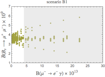
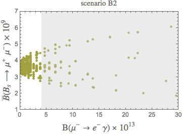
𝓑(𝝁𝒆𝜸)4.2×𝟏𝟎𝟏𝟑,𝓑bold-→𝝁𝒆𝜸4.2superscript1013\mathcal{B}(\mu\to e\gamma)\leq 4.2\times 10^{-13}, (97)

and [42]

𝓑(𝝉𝝁𝜸)4.4×𝟏𝟎𝟖,𝓑(𝝉𝒆𝜸)3.3×𝟏𝟎𝟖.formulae-sequence𝓑bold-→𝝉𝝁𝜸4.4superscript108𝓑bold-→𝝉𝒆𝜸3.3superscript108\mathcal{B}(\tau\to\mu\gamma)\leq 4.4\times 10^{-8},\qquad\mathcal{B}(\tau\to e\gamma)\leq 3.3\times 10^{-8}\,. (98)

4.3 Three-body Lepton decays

For a decay 𝒋𝒊¯𝒍𝒌bold-→subscriptbold-ℓ𝒋subscriptbold-ℓ𝒊subscriptbold-¯bold-ℓ𝒍subscriptbold-ℓ𝒌\ell_{j}\to\ell_{i}\bar{\ell}_{l}\ell_{k} we have the following contributing operators and their Wilson coefficients with 𝑿,𝒀=𝑳,𝑹formulae-sequence𝑿𝒀𝑳𝑹X,Y=L,R

[𝑸𝑽𝑿𝒀]𝒌𝒍𝒊𝒋=(𝝍¯𝒊𝜸𝝁𝑷𝑿𝝍𝒋)(𝝍¯𝒌𝜸𝝁𝑷𝒀𝝍𝒍),[𝑪𝑽𝑿𝒀]𝒌𝒍𝒊𝒋=𝚫𝑿𝒊𝒋(𝒁)𝚫𝒀𝒌𝒍(𝒁)𝑴𝒁𝟐.formulae-sequencesubscriptsuperscriptdelimited-[]subscript𝑸𝑽𝑿𝒀𝒊𝒋𝒌𝒍subscriptbold-¯𝝍𝒊superscript𝜸𝝁subscript𝑷𝑿subscript𝝍𝒋subscriptbold-¯𝝍𝒌subscript𝜸𝝁subscript𝑷𝒀subscript𝝍𝒍subscriptsuperscriptdelimited-[]subscript𝑪𝑽𝑿𝒀𝒊𝒋𝒌𝒍subscriptsuperscript𝚫𝒊𝒋𝑿superscript𝒁bold-′subscriptsuperscript𝚫𝒌𝒍𝒀superscript𝒁bold-′subscriptsuperscript𝑴2superscript𝒁bold-′[Q_{VXY}]^{ij}_{kl}=(\bar{\psi}_{i}\gamma^{\mu}P_{X}\psi_{j})(\bar{\psi}_{k}\gamma_{\mu}P_{Y}\psi_{l})\,,\qquad[C_{VXY}]^{ij}_{kl}=\frac{\Delta^{ij}_{X}(Z^{\prime})\Delta^{kl}_{Y}(Z^{\prime})}{M^{2}_{Z^{\prime}}}. (99)

Calculating the branching ratios for the most interesting decays with 𝒌=𝒍𝒌𝒍k=l we have to take into account the presence of two identical leptons in the final state that requires the introduction of a factor 𝟏/𝟐121/2 at the level of the branching ratio. Moreover always two diagrams, differing by the interchange of identical leptons, contribute. They interfere with each other for 𝑽𝑳𝑳𝑽𝑳𝑳VLL and 𝑽𝑹𝑹𝑽𝑹𝑹VRR cases but not for 𝑽𝑳𝑹𝑽𝑳𝑹VLR and 𝑽𝑹𝑳𝑽𝑹𝑳VRL. We find then

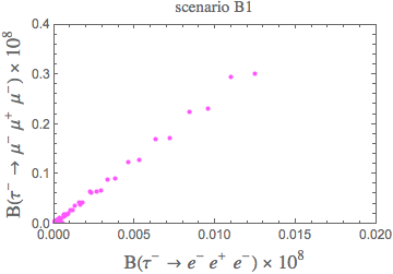
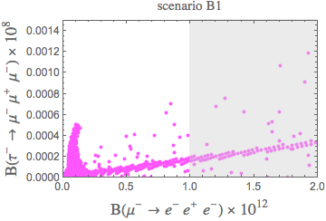
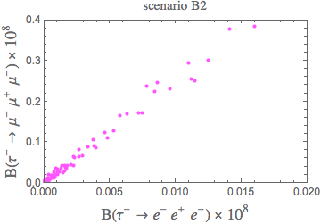
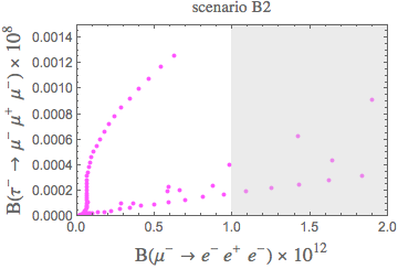
𝓑(𝝉𝝁𝝁+𝝁)=𝒎𝝉𝟓𝟏𝟓𝟑𝟔𝝅𝟑𝚪𝝉[𝟐|𝑪𝑽𝑳𝑳|𝟐+𝟐|𝑪𝑽𝑹𝑹|𝟐+|𝑪𝑽𝑳𝑹|𝟐+|𝑪𝑽𝑹𝑳|𝟐]𝝁𝝁𝝁𝝉,𝓑bold-→superscript𝝉superscript𝝁superscript𝝁superscript𝝁superscriptsubscript𝒎𝝉51536superscript𝝅3subscript𝚪𝝉subscriptsuperscriptdelimited-[]2superscriptsubscript𝑪𝑽𝑳𝑳22superscriptsubscript𝑪𝑽𝑹𝑹2superscriptsubscript𝑪𝑽𝑳𝑹2superscriptsubscript𝑪𝑽𝑹𝑳2𝝁𝝉𝝁𝝁\mathcal{B}(\tau^{-}\to\mu^{-}\mu^{+}\mu^{-})=\frac{m_{\tau}^{5}}{1536\pi^{3}\Gamma_{\tau}}\left[2|C_{VLL}|^{2}+2|C_{VRR}|^{2}+|C_{VLR}|^{2}+|C_{VRL}|^{2}\right]^{\mu\tau}_{\mu\mu}\,, (100)

with analogous expressions for 𝝁𝒆𝒆+𝒆bold-→superscript𝝁superscript𝒆superscript𝒆superscript𝒆\mu^{-}\to e^{-}e^{+}e^{-} and 𝝉𝒆𝒆+𝒆bold-→superscript𝝉superscript𝒆superscript𝒆superscript𝒆\tau^{-}\to e^{-}e^{+}e^{-}. 𝚪𝝉subscript𝚪𝝉\Gamma_{\tau} is the total 𝝉𝝉\tau decay width. This formula agrees with the one in [43, 44], and can also be derived from the expressions in [45] with the factors of 2, exhibited here, hidden in the Wilson coefficients.

Present bounds are [46]:

𝓑(𝝉𝝁𝝁+𝝁)𝓑bold-→superscript𝝉superscript𝝁superscript𝝁superscript𝝁\displaystyle\mathcal{B}(\tau^{-}\to\mu^{-}\mu^{+}\mu^{-}) <\displaystyle< 1.2𝟏𝟎𝟖,bold-⋅1.2superscript108\displaystyle 1.2\cdot 10^{-8}\,, (101)
𝓑(𝝉𝒆𝒆+𝒆)𝓑bold-→superscript𝝉superscript𝒆superscript𝒆superscript𝒆\displaystyle\mathcal{B}(\tau^{-}\to e^{-}e^{+}e^{-}) <\displaystyle< 1.4𝟏𝟎𝟖,bold-⋅1.4superscript108\displaystyle 1.4\cdot 10^{-8}\,, (102)
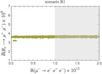
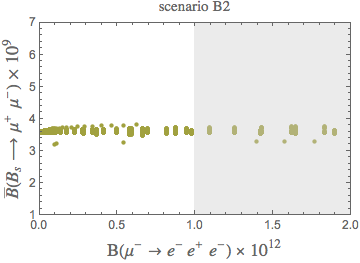
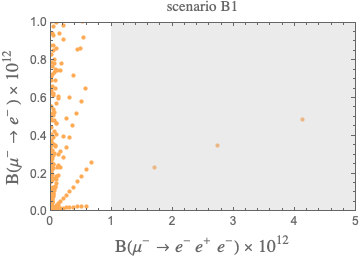
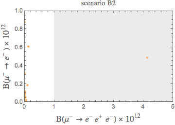
𝓑(𝝁𝒆𝒆+𝒆)𝓑bold-→superscript𝝁superscript𝒆superscript𝒆superscript𝒆\displaystyle\mathcal{B}(\mu^{-}\to e^{-}e^{+}e^{-}) <\displaystyle< 1.0𝟏𝟎𝟏𝟐,bold-⋅1.0superscript1012\displaystyle 1.0\cdot 10^{-12}\,,\,\, (103)

that update the more conservative PDG bounds [47].

4.4 𝝁𝒆𝝁𝒆{\mu-e} conversion in nuclei

We give next the formula for the 𝝁𝝁\mu-𝒆𝒆e conversion in nuclei, that is

𝝁+(𝑨,𝒁)𝒆+(𝑨,𝒁),bold-→𝝁𝑨𝒁𝒆𝑨𝒁\mu+(A,Z)\rightarrow e+(A,Z)\,, (104)

where 𝒁𝒁Z and 𝑨𝑨A denote the proton and atomic numbers in a nucleus, respectively. Adapting general formulae in [48] and keeping the dominant tree-level contributions we find

𝚪(𝝁𝒆)𝚪bold-→𝝁𝒆\displaystyle\Gamma(\mu\rightarrow e) =\displaystyle= 𝜶𝟑𝟏𝟔𝝅𝟐𝒁𝒆𝒇𝒇𝟒𝒁|𝑭(𝒒)|𝟐𝒎𝝁𝟓𝑴𝒁𝟒[|𝚫𝑳𝝁𝒆(𝒁)|𝟐+|𝚫𝑹𝝁𝒆(𝒁)|𝟐]superscript𝜶316superscript𝝅2superscriptsubscript𝒁𝒆𝒇𝒇4𝒁superscript𝑭𝒒2superscriptsubscript𝒎𝝁5subscriptsuperscript𝑴4superscript𝒁bold-′delimited-[]superscriptsuperscriptsubscript𝚫𝑳𝝁𝒆superscript𝒁bold-′2superscriptsuperscriptsubscript𝚫𝑹𝝁𝒆superscript𝒁bold-′2\displaystyle\frac{\alpha^{3}}{16\pi^{2}}\frac{Z_{eff}^{4}}{Z}|F(q)|^{2}~{}\frac{m_{\mu}^{5}}{M^{4}_{Z^{\prime}}}\left[|\Delta_{L}^{\mu e}(Z^{\prime})|^{2}+|\Delta_{R}^{\mu e}(Z^{\prime})|^{2}\right] (105)
×|(𝟐𝒁+𝑵)𝚫𝑽𝒖𝒖(𝒁)+(𝒁+𝟐𝑵)𝚫𝑽𝒅𝒅(𝒁)|𝟐,absentsuperscript2𝒁𝑵superscriptsubscript𝚫𝑽𝒖𝒖superscript𝒁bold-′𝒁2𝑵superscriptsubscript𝚫𝑽𝒅𝒅superscript𝒁bold-′2\displaystyle\times|(2Z+N)\Delta_{V}^{uu}(Z^{\prime})+(Z+2N)\Delta_{V}^{dd}(Z^{\prime})|^{2},

with 𝚫𝑽𝒊𝒋subscriptsuperscript𝚫𝒊𝒋𝑽\Delta^{ij}_{V} given in (96). 𝒁𝒁Z and 𝑵𝑵N denote the proton and neutron numbers in a nucleus, respectively. 𝒁𝒆𝒇𝒇subscript𝒁𝒆𝒇𝒇Z_{eff} is an effective parameter and 𝑭(𝒒𝟐)𝑭superscript𝒒2F(q^{2}) the nuclear form factor. The branching ratio used by experimentalists is defined by

𝓑(𝝁𝒆)=𝚪(𝝁𝒆)𝚪𝐜𝐚𝐩𝐭,𝓑bold-→𝝁𝒆𝚪bold-→𝝁𝒆subscript𝚪𝐜𝐚𝐩𝐭\mathcal{B}(\mu\to e)=\frac{\Gamma(\mu\rightarrow e)}{\Gamma_{\rm capt}}\,, (106)

where 𝚪𝐜𝐚𝐩𝐭subscript𝚪𝐜𝐚𝐩𝐭\Gamma_{\rm capt} is the muon capture rate. For the case of 𝐓𝐢𝟐𝟐𝟒𝟖superscriptsubscript𝐓𝐢2248{}^{48}_{22}{\rm{Ti}}, one finds 𝒁𝒆𝒇𝒇=17.6subscript𝒁𝒆𝒇𝒇17.6Z_{eff}=17.6 and 𝑭(𝒒𝟐𝒎𝝁𝟐)0.54similar-to-or-equals𝑭similar-to-or-equalssuperscript𝒒2superscriptsubscript𝒎𝝁20.54F(q^{2}\simeq-m_{\mu}^{2})\simeq 0.54 [49] and 𝚪𝐜𝐚𝐩𝐭(2.590±0.012)𝟏𝟎𝟔/𝒔similar-to-or-equalssubscript𝚪𝐜𝐚𝐩𝐭bold-⋅plus-or-minus2.5900.012superscript106𝒔\Gamma_{\rm capt}\simeq(2.590\pm 0.012)\cdot 10^{6}/s [50]. The present experimental bound for the branching ratio reads [51]

𝓑(𝝁𝒆)𝓞(𝟏𝟎𝟏𝟐).𝓑bold-→𝝁𝒆𝓞superscript1012\mathcal{B}(\mu\to e)\leq\mathcal{O}(10^{-12})\,. (107)

4.5 (𝒈𝟐)𝝁subscript𝒈2𝝁(g-2)_{\mu} and (𝒈𝟐)𝒆subscript𝒈2𝒆(g-2)_{e}

Using general formulae in [40] we find for 𝒂𝝁=(𝒈𝟐)𝝁/𝟐subscript𝒂𝝁subscript𝒈2𝝁2a_{\mu}=(g-2)_{\mu}/2

𝚫𝒂𝝁(𝒁)𝟏𝟏𝟔𝝅𝟐𝒎𝝁𝟐𝑴𝒁𝟐𝒇=𝒆,𝝁,𝝉[|𝚫𝑽𝒇𝝁(𝒁)|𝟐(𝟐𝟑𝒎𝒇𝒎𝝁)+|𝚫𝑨𝒇𝝁(𝒁)|𝟐(𝟐𝟑+𝒎𝒇𝒎𝝁)]𝚫subscript𝒂𝝁superscript𝒁bold-′116superscript𝝅2superscriptsubscript𝒎𝝁2subscriptsuperscript𝑴2superscript𝒁bold-′subscript𝒇𝒆𝝁𝝉delimited-[]superscriptsubscriptsuperscript𝚫𝒇𝝁𝑽superscript𝒁bold-′223subscript𝒎𝒇subscript𝒎𝝁superscriptsubscriptsuperscript𝚫𝒇𝝁𝑨superscript𝒁bold-′223subscript𝒎𝒇subscript𝒎𝝁\Delta a_{\mu}(Z^{\prime})\approx-\frac{1}{16\pi^{2}}\frac{m_{\mu}^{2}}{M^{2}_{Z^{\prime}}}\sum_{f=e,\mu,\tau}\left[\left|\Delta^{f\mu}_{V}(Z^{\prime})\right|^{2}\left(\frac{2}{3}-\frac{m_{f}}{m_{\mu}}\right)+\left|\Delta^{f\mu}_{A}(Z^{\prime})\right|^{2}\left(\frac{2}{3}+\frac{m_{f}}{m_{\mu}}\right)\right] (108)

with 𝚫𝑽𝒊𝒋subscriptsuperscript𝚫𝒊𝒋𝑽\Delta^{ij}_{V} and 𝚫𝑨𝒊𝒋subscriptsuperscript𝚫𝒊𝒋𝑨\Delta^{ij}_{A} given in (96). The summation is over internal charged leptons in the loop. This result is also valid for new heavy charged leptons provided 𝒎𝒇/𝑴𝒁0.2subscript𝒎𝒇subscript𝑴superscript𝒁bold-′0.2m_{f}/M_{Z^{\prime}}\leq 0.2. For heavier leptons exact expressions in [40] have to be used. For (𝒈𝟐)𝒆subscript𝒈2𝒆(g-2)_{e} one just replaces 𝝁𝝁\mu by 𝒆𝒆e.

5 Various coupling scenarios

5.1 Preliminaries and general strategy for numerics

In Section 3 we have derived the couplings of the 𝒁superscript𝒁bold-′Z^{\prime} to SM quarks and leptons as well as to RH neutrinos assuming that they are Dirac particles.

It should be recalled that the parameters ϵ𝒊subscriptbold-italic-ϵ𝒊\epsilon_{i} are the same in the quark and lepton sectors which in our simple model is a direct consequence of the cancellation of gauge anomalies. This then implies that we should expect correlations between various observables not only separately within the lepton and quark systems but in particular between lepton and quark observables.

Before entering numerics it is strategically useful to count the full number of free parameters and subsequently define a few simple scenarios in which some of these parameters vanish. In this manner the number of correlations between various observables is increased.

Let us then count the number of free parameters:

  • 4 real parameters entering both quark and lepton couplings

    𝒈𝒁,𝑴𝒁,ϵ𝟏,ϵ𝟐.subscript𝒈superscript𝒁bold-′subscript𝑴superscript𝒁bold-′subscriptbold-italic-ϵ1subscriptbold-italic-ϵ2g_{Z^{\prime}},\qquad M_{Z^{\prime}},\qquad\epsilon_{1},\qquad\epsilon_{2}\,. (109)

    Even if all formulae listed above depend only on the ratio 𝒈𝒁/𝑴𝒁subscript𝒈superscript𝒁bold-′subscript𝑴superscript𝒁bold-′g_{Z^{\prime}}/M_{Z^{\prime}}, the renormalization group effects depend only on 𝑴𝒁subscript𝑴superscript𝒁bold-′M_{Z^{\prime}} and these are two independent parameters.

  • 1 complex phase in the PMNS matrix in LH couplings. The remaining parameters in the latter couplings are already measured parameters of the CKM and PMNS matrices.

  • 3 mixing angles and three complex phases in RH quark couplings:

    (𝒔~𝟏𝟐,ϕ𝑲),(𝒔~𝟏𝟑,ϕ𝒅),(𝒔~𝟐𝟑,ϕ𝒔).subscriptbold-~𝒔12subscriptbold-italic-ϕ𝑲subscriptbold-~𝒔13subscriptbold-italic-ϕ𝒅subscriptbold-~𝒔23subscriptbold-italic-ϕ𝒔(\tilde{s}_{12},\,\phi_{K}),\qquad(\tilde{s}_{13},\,\phi_{d}),\qquad(\tilde{s}_{23},\,\phi_{s}). (110)
  • 3 mixing angles and three complex phases in RH lepton couplings:

    (𝒕~𝟏𝟐,ϕ𝟏𝟐),(𝒕~𝟏𝟑,ϕ𝟏𝟑),(𝒕~𝟐𝟑,ϕ𝟐𝟑).subscriptbold-~𝒕12subscriptbold-italic-ϕ12subscriptbold-~𝒕13subscriptbold-italic-ϕ13subscriptbold-~𝒕23subscriptbold-italic-ϕ23(\tilde{t}_{12},\,\phi_{12}),\qquad(\tilde{t}_{13},\,\phi_{13}),\qquad(\tilde{t}_{23},\,\phi_{23}). (111)

We observe then that in full generality we have 10 real parameters and 6 phases to our disposal. This could appear as very many. Yet, by considering 𝑲𝑲K, 𝑩𝒅subscript𝑩𝒅B_{d} and 𝑩𝒔subscript𝑩𝒔B_{s} meson systems with 𝚫𝑭=𝟏𝚫𝑭1\Delta F=1 and 𝚫𝑭=𝟐𝚫𝑭2\Delta F=2 transitions and the charged lepton flavour violating decays, 𝝁𝒆𝝁𝒆\mu-e conversion as well as (𝒈𝟐)𝒆,𝝁subscript𝒈2𝒆𝝁(g-2)_{e,\mu}, there is a sufficient number of observables so that not only the parameters in question can be bounded but also correlations between various observables can be predicted.

In what follows, we will consider four constrained scenarios. Except for the last one, we will adopt a common strategy for numerics. We will perform a simplified analysis of 𝚫𝑭=𝟐𝚫𝑭2\Delta F=2 observables. The relevant formulae for these when a new 𝒁superscript𝒁bold-′Z^{\prime} gauge boson is present can be found in Section 3.3 of [3] to which we address the reader. We consider in the Kaon sector 𝜺𝑲subscript𝜺𝑲\varepsilon_{K} and in the 𝑩𝒅,𝒔subscript𝑩𝒅𝒔B_{d,s} sectors the neutral meson mass differences 𝚫𝑴𝒅,𝒔𝚫subscript𝑴𝒅𝒔\Delta M_{d,s}, as well, as the CP asymmetries 𝑺𝝍𝑲𝑺subscript𝑺𝝍subscript𝑲𝑺S_{\psi K_{S}} and 𝑺𝝍ϕsubscript𝑺𝝍bold-italic-ϕS_{\psi\phi} in order to identify oases in the space of new parameters discussed in the previous section for which these five observables are consistent with experiment. To this end, we set all other input parameters at their central values. But to take partially hadronic and experimental uncertainties into account we require the theory to reproduce the data for 𝜺𝑲subscript𝜺𝑲\varepsilon_{K} within ±𝟏𝟎%plus-or-minuspercent10\pm 10\%, 𝚫𝑴𝒔,𝒅𝚫subscript𝑴𝒔𝒅\Delta M_{s,d} within ±𝟓%plus-or-minuspercent5\pm 5\% and the data on 𝑺𝝍𝑲𝑺subscript𝑺𝝍subscript𝑲𝑺S_{\psi K_{S}} and 𝑺𝝍ϕsubscript𝑺𝝍bold-italic-ϕS_{\psi\phi} within experimental 𝟐𝝈2𝝈2\sigma. We choose a larger uncertainty for 𝜺𝑲subscript𝜺𝑲\varepsilon_{K} than for 𝚫𝑴𝒔,𝒅𝚫subscript𝑴𝒔𝒅\Delta M_{s,d} because of its strong |𝑽𝒄𝒃|𝟒superscriptsubscript𝑽𝒄𝒃4|V_{cb}|^{4} dependence. For the neutral Kaon mass difference 𝚫𝑴𝑲𝚫subscript𝑴𝑲\Delta M_{K} we will only require the agreement within ±𝟐𝟓%plus-or-minuspercent25\pm 25\% because of potential long distance uncertainties.

Specifically, our search is governed by the following allowed ranges:

16.0/𝐩𝐬𝚫𝑴𝒔19.5/𝐩𝐬,0.01𝑺𝝍ϕ0.10,formulae-sequence16.0𝐩𝐬𝚫subscript𝑴𝒔19.5𝐩𝐬0.01subscript𝑺𝝍bold-italic-ϕ0.1016.0/{\rm ps}\leq\Delta M_{s}\leq 19.5/{\rm ps},\quad 0.01\leq S_{\psi\phi}\leq 0.10, (112)
0.455/𝐩𝐬𝚫𝑴𝒅0.556/𝐩𝐬,0.665𝑺𝝍𝑲𝑺0.733.formulae-sequence0.455𝐩𝐬𝚫subscript𝑴𝒅0.556𝐩𝐬0.665subscript𝑺𝝍subscript𝑲𝑺0.7330.455/{\rm ps}\leq\Delta M_{d}\leq 0.556/{\rm ps},\quad 0.665\leq S_{\psi K_{S}}\leq 0.733. (113)
0.75𝚫𝑴𝑲(𝚫𝑴𝑲)𝐒𝐌1.25,2.0×𝟏𝟎𝟑|𝜺𝑲|2.5×𝟏𝟎𝟑.formulae-sequence0.75𝚫subscript𝑴𝑲subscript𝚫subscript𝑴𝑲𝐒𝐌1.252.0superscript103subscript𝜺𝑲2.5superscript1030.75\leq\frac{\Delta M_{K}}{(\Delta M_{K})_{\rm SM}}\leq 1.25,\qquad 2.0\times 10^{-3}\leq|\varepsilon_{K}|\leq 2.5\times 10^{-3}. (114)

Moreover, in the Kaon sector, we impose that the short-distance contribution to the 𝓑(𝑲𝑳𝝁+𝝁)𝓑bold-→subscript𝑲𝑳superscript𝝁superscript𝝁{\cal B}(K_{L}\to\mu^{+}\mu^{-}) satisfies the bound [52]:

𝓑(𝑲𝑳𝝁+𝝁)𝑺𝑫<2.5𝟏𝟎𝟗.𝓑subscriptbold-→subscript𝑲𝑳superscript𝝁superscript𝝁𝑺𝑫bold-⋅2.5superscript109{\cal B}(K_{L}\to\mu^{+}\mu^{-})_{SD}<2.5\cdot 10^{-9}\,\,. (115)

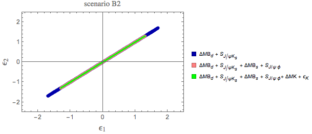
In what follows, we will first identify the region in the space of the parameters ϵ𝟏subscriptbold-italic-ϵ1\epsilon_{1} and ϵ𝟐subscriptbold-italic-ϵ2\epsilon_{2} allowed by the constraints in (112)-(114) for each scenario. Subsequently, we will investigate correlations between various observables in this region.

For the numerical analysis of the model of Section 3 we consider a relatively light 𝒁superscript𝒁bold-′Z^{\prime} setting 𝑴𝒁=𝟏subscript𝑴superscript𝒁bold-′1M_{Z^{\prime}}=1 TeV and we vary the gauge coupling in the range 𝒈𝒁[0.01, 1]subscript𝒈superscript𝒁bold-′0.011g_{Z^{\prime}}\in[0.01,\,1]. This will allow us to neglect RG effects from Yukawa and electroweak interactions that could also imply correlations between observables, thereby exhibiting the correlations implied by the cancellation of gauge anomalies. Therefore, as already stated above, the matching is performed directly onto the WET below the EW scale and only QCD RG effects are taken into account. We summarize our intput in Tables 1 and 2.

𝑮𝑭=1.16637(𝟏)×𝟏𝟎𝟓𝐆𝐞𝐕𝟐subscript𝑮𝑭1.166371superscript105superscript𝐆𝐞𝐕2G_{F}=1.16637(1)\times 10^{-5}\,{\rm GeV}^{-2} 𝑴𝒁=91.188(𝟐)𝐆𝐞𝐕subscript𝑴𝒁91.1882𝐆𝐞𝐕M_{Z}=91.188(2)\,{\rm GeV} 𝑴𝑾=80.385(𝟏𝟓)𝐆𝐞𝐕subscript𝑴𝑾80.38515𝐆𝐞𝐕M_{W}=80.385(15)\,{\rm GeV}
𝐬𝐢𝐧𝟐𝜽𝑾=0.23116(𝟏𝟑)superscript2subscript𝜽𝑾0.2311613\sin^{2}\theta_{W}=0.23116(13) 𝜶(𝑴𝒁)=𝟏/127.94𝜶subscript𝑴𝒁1127.94\alpha(M_{Z})=1/127.94 𝜶𝒔(𝑴𝒁)=0.1184(𝟕)subscript𝜶𝒔subscript𝑴𝒁0.11847\alpha_{s}(M_{Z})=0.1184(7)
𝒎𝒆=0.511𝐌𝐞𝐕subscript𝒎𝒆0.511𝐌𝐞𝐕m_{e}=0.511\,{\rm MeV} 𝒎𝝁=105.66𝐌𝐞𝐕subscript𝒎𝝁105.66𝐌𝐞𝐕m_{\mu}=105.66\,{\rm MeV} 𝒎𝝉=1776.9(𝟏)𝐌𝐞𝐕subscript𝒎𝝉1776.91𝐌𝐞𝐕m_{\tau}=1776.9(1)\,{\rm MeV}
𝒎𝒖(𝟐𝐆𝐞𝐕)=2.16(𝟏𝟏)𝐌𝐞𝐕subscript𝒎𝒖2𝐆𝐞𝐕2.1611𝐌𝐞𝐕m_{u}(2\,{\rm GeV})=2.16(11)\,{\rm MeV} 𝒎𝒄(𝒎𝒄)=1.279(𝟏𝟑)𝐆𝐞𝐕subscript𝒎𝒄subscript𝒎𝒄1.27913𝐆𝐞𝐕m_{c}(m_{c})=1.279(13)\,{\rm GeV} 𝒎𝒕(𝒎𝒕)=𝟏𝟔𝟑(𝟏)𝐆𝐞𝐕subscript𝒎𝒕subscript𝒎𝒕1631𝐆𝐞𝐕m_{t}(m_{t})=163(1)\,{\rm GeV}
𝒎𝒅(𝟐𝐆𝐞𝐕)=4.68(𝟏𝟓)𝐌𝐞𝐕subscript𝒎𝒅2𝐆𝐞𝐕4.6815𝐌𝐞𝐕m_{d}(2\,{\rm GeV})=4.68(15)\,{\rm MeV} 𝒎𝒔(𝟐𝐆𝐞𝐕)=93.8(𝟐𝟒)𝐌𝐞𝐕subscript𝒎𝒔2𝐆𝐞𝐕93.824𝐌𝐞𝐕m_{s}(2\,{\rm GeV})=93.8(24)\,{\rm MeV} 𝒎𝒃(𝒎𝒃)=4.190.06+0.18𝐆𝐞𝐕subscript𝒎𝒃subscript𝒎𝒃subscriptsuperscript4.190.180.06𝐆𝐞𝐕m_{b}(m_{b})=4.19^{+0.18}_{-0.06}\,{\rm GeV}
𝒎𝑲±=493.68(𝟐)𝐌𝐞𝐕subscript𝒎superscript𝑲plus-or-minus493.682𝐌𝐞𝐕m_{K^{\pm}}=493.68(2)\,{\rm MeV} 𝒎𝑲𝟎=497.61(𝟏)𝐌𝐞𝐕subscript𝒎superscript𝑲0497.611𝐌𝐞𝐕m_{K^{0}}=497.61(1)\,{\rm MeV}
𝒎𝑩𝒅=5279.62(𝟏𝟓)𝐌𝐞𝐕subscript𝒎subscript𝑩𝒅5279.6215𝐌𝐞𝐕m_{B_{d}}=5279.62(15)\,{\rm MeV} 𝒎𝑩𝒔=5366.82(𝟐𝟐)𝐌𝐞𝐕subscript𝒎subscript𝑩𝒔5366.8222𝐌𝐞𝐕m_{B_{s}}=5366.82(22)\,{\rm MeV}
𝚫𝑴𝑲=0.5292(𝟗)×𝟏𝟎𝟐ps𝟏𝚫subscript𝑴𝑲0.52929superscript102superscriptps1\Delta M_{K}=0.5292(9)\times 10^{-2}\,\text{ps}^{-1} 𝚫𝑴𝒅=0.5055(𝟐𝟎)ps𝟏𝚫subscript𝑴𝒅0.505520superscriptps1\Delta M_{d}=0.5055(20)\,\text{ps}^{-1} 𝚫𝑴𝒔=17.757(𝟐𝟏)ps𝟏𝚫subscript𝑴𝒔17.75721superscriptps1\Delta M_{s}=17.757(21)\,\text{ps}^{-1}
|ϵ𝑲|=2.228(𝟏𝟏)×𝟏𝟎𝟑subscriptbold-italic-ϵ𝑲2.22811superscript103|\epsilon_{K}|=2.228(11)\times 10^{-3} 𝑺𝝍𝑲𝑺=0.699(𝟏𝟕)subscript𝑺𝝍subscript𝑲𝑺0.69917S_{\psi K_{S}}=0.699(17) 𝑺𝝍ϕ=0.054(𝟐𝟎)subscript𝑺𝝍bold-italic-ϕ0.05420S_{\psi\phi}=0.054(20)
𝐬𝐢𝐧𝟐(𝜽𝟏𝟐)=0.307±0.013superscript2subscript𝜽12plus-or-minus0.3070.013\sin^{2}\left(\theta_{12}\right)=0.307\pm 0.013 𝐬𝐢𝐧𝟐(𝜽𝟐𝟑)=0.506±0.04superscript2subscript𝜽23plus-or-minus0.5060.04\sin^{2}\left(\theta_{23}\right)=0.506\pm 0.04 𝐬𝐢𝐧𝟐(𝜽𝟏𝟑)=0.0212±0.0008superscript2subscript𝜽13plus-or-minus0.02120.0008\sin^{2}\left(\theta_{13}\right)=0.0212\pm 0.0008
Table 1: Values of theoretical quantities used for the numerical analysis.
𝑭𝑩𝒅subscript𝑭subscript𝑩𝒅F_{B_{d}} = 190.5(𝟏𝟑)𝐌𝐞𝐕190.513𝐌𝐞𝐕190.5(13)\,{\rm MeV} 𝑭𝑩𝒔subscript𝑭subscript𝑩𝒔F_{B_{s}} = 230.7(𝟏𝟐)𝐌𝐞𝐕230.712𝐌𝐞𝐕230.7(12)\,{\rm MeV} 𝑭𝑲=156.1(𝟏𝟏)𝐌𝐞𝐕subscript𝑭𝑲156.111𝐌𝐞𝐕F_{K}=156.1(11)\,{\rm MeV}
𝑩^𝑩𝒅=1.232(𝟓𝟑)subscriptbold-^𝑩subscript𝑩𝒅1.23253\hat{B}_{B_{d}}=1.232(53) 𝑩^𝑩𝒔=1.222(𝟔𝟏)subscriptbold-^𝑩subscript𝑩𝒔1.22261\hat{B}_{B_{s}}=1.222(61) 𝑩^𝑲=0.766(𝟏𝟎)subscriptbold-^𝑩𝑲0.76610\hat{B}_{K}=0.766(10)
𝑭𝑩𝒅𝑩^𝑩𝒅=210.6(𝟓𝟓)𝐌𝐞𝐕subscript𝑭subscript𝑩𝒅subscriptbold-^𝑩subscript𝑩𝒅210.655𝐌𝐞𝐕F_{B_{d}}\sqrt{\hat{B}_{B_{d}}}=210.6(55)\,{\rm MeV} 𝑭𝑩𝒔𝑩^𝑩𝒔=256.1(𝟓𝟕)𝐌𝐞𝐕subscript𝑭subscript𝑩𝒔subscriptbold-^𝑩subscript𝑩𝒔256.157𝐌𝐞𝐕F_{B_{s}}\sqrt{\hat{B}_{B_{s}}}=256.1(57)\,{\rm MeV} 𝝃=1.21(𝟐)𝝃1.212\xi=1.21(2)
𝜼𝒄𝒄=1.87(𝟕𝟔)subscript𝜼𝒄𝒄1.8776\eta_{cc}=1.87(76) 𝜼𝒄𝒕=0.496(𝟒𝟕)subscript𝜼𝒄𝒕0.49647\eta_{ct}=0.496(47) 𝜼𝒕𝒕=0.5765(𝟔𝟓)subscript𝜼𝒕𝒕0.576565\eta_{tt}=0.5765(65)
𝜼𝑩=0.55(𝟏)subscript𝜼𝑩0.551\eta_{B}=0.55(1) ϕϵ=43.51(𝟓)subscriptbold-italic-ϕbold-italic-ϵ43.51superscript5\phi_{\epsilon}=43.51(5)^{\circ} 𝜿ϵ=0.94(𝟐)subscript𝜿bold-italic-ϵ0.942\kappa_{\epsilon}=0.94(2)
|𝑽𝒖𝒔|=0.2254(𝟒)subscript𝑽𝒖𝒔0.22544|V_{us}|=0.2254(4) |𝑽𝒖𝒃nom|=3.7×𝟏𝟎𝟑subscriptsuperscript𝑽nom𝒖𝒃3.7superscript103|V^{\text{nom}}_{ub}|=3.7\times 10^{-3} |𝑽𝒄𝒃nom|=42.0×𝟏𝟎𝟑subscriptsuperscript𝑽nom𝒄𝒃42.0superscript103|V^{\text{nom}}_{cb}|=42.0\times 10^{-3}
Table 2: Numerical values used for the numerical analysis.

5.2 Different Scenarios

We will consider a number of different scenarios that we want to describe briefly here.

5.2.1 Scenario A

In this scenario flavour violation is present only in the LH couplings. This is achieved by setting all parameters 𝒔~𝒊𝒋subscriptbold-~𝒔𝒊𝒋\tilde{s}_{ij} and 𝒕~𝒊𝒋subscriptbold-~𝒕𝒊𝒋\tilde{t}_{ij} to zero such that all flavour-violating RH couplings vanish. This leaves us with only four real parameters in (109) and the PMNS phase.

It should be noted that the flavour conserving RH couplings are generally non-zero. In fact inspecting the formulae for these couplings, it is clear that it is impossible to set them all to zero.

There are two important implications of this structure:

  • The absence of RH flavour-violating couplings implies the absence of left-right operators contributing to 𝚫𝑭=𝟐𝚫𝑭2\Delta F=2 processes. As the hadronic matrix elements of these operators are, in particular in the case of the 𝑲𝟎𝑲¯𝟎superscript𝑲0superscriptbold-¯𝑲0K^{0}-\bar{K}^{0} system, strongly enhanced, their absence allows to satisfy constraints from 𝜺𝑲subscript𝜺𝑲\varepsilon_{K} and the mass differences 𝚫𝑴𝑲𝚫subscript𝑴𝑲\Delta M_{K}, 𝚫𝑴𝒅𝚫subscript𝑴𝒅\Delta M_{d} and 𝚫𝑴𝒔𝚫subscript𝑴𝒔\Delta M_{s} easier than in the subsequent scenarios.

  • Non-vanishing flavour conserving RH currents together with flavour-violating LH currents imply the presence of the dominant QCD (𝑸𝟔)subscript𝑸6(Q_{6}) and electroweak penguin (𝑸𝟖)subscript𝑸8(Q_{8}) operators contributing to 𝜺/𝜺superscript𝜺bold-′𝜺\varepsilon^{\prime}/\varepsilon thereby allowing to address the 𝜺/𝜺superscript𝜺bold-′𝜺\varepsilon^{\prime}/\varepsilon-anomaly.

  • Moreover the small number of free parameters implies a number of correlations.

5.2.2 Scenarios B1 and B2

In these scenarios flavour violation is present in both LH and RH quark currents, but for leptons only in LH currents. At first sight six additional parameters in (110) enter the phenomenology. However, the presence of left-right operators implies that it is very difficult to satisfy the constraints in the 𝑲𝟎𝑲¯𝟎superscript𝑲0superscriptbold-¯𝑲0K^{0}-\bar{K}^{0} mixing for 𝑴𝒁=𝓞(𝟏𝐓𝐞𝐕)subscript𝑴superscript𝒁bold-′𝓞1𝐓𝐞𝐕M_{Z^{\prime}}=\mathcal{O}(1\,{\rm TeV}), so that, the 𝚫𝑹𝒔𝒅superscriptsubscript𝚫𝑹𝒔𝒅\Delta_{R}^{sd} coupling has to be strongly suppressed or even eliminated. This can be done by setting

𝒔~𝟏𝟐=𝟎,(Scenario B1)formulae-sequencebold-∙subscriptbold-~𝒔120Scenario B1\bullet\hskip 113.81102pt\tilde{s}_{12}=0,\qquad(\text{Scenario B1}) (116)

or

ϵ𝟏=ϵ𝟐,(Scenario B2).formulae-sequencebold-∙subscriptbold-italic-ϵ1subscriptbold-italic-ϵ2Scenario B2\bullet\hskip 113.81102pt\epsilon_{1}=\epsilon_{2},\qquad(\text{Scenario B2}). (117)

In both scenarios only four additional parameters relative to Scenario A are present. Moreover, in Scenario B2 the number of free parameters is reduced through the relation ϵ𝟏=ϵ𝟐subscriptbold-italic-ϵ1subscriptbold-italic-ϵ2\epsilon_{1}=\epsilon_{2}.

5.2.3 Scenario C

In this scenario, with both LH and RH currents, it is possible, as explained in the Appendix A, to eliminate 𝚫𝑭=𝟐𝚫𝑭2\Delta F=2 constraints in Kaon and 𝑩𝒔,𝒅subscript𝑩𝒔𝒅B_{s,d} systems which allows to obtain larger NP effects in 𝚫𝑭=𝟏𝚫𝑭1\Delta F=1 transitions. This allows to see the correlations between various observables in different systems even better than in the previous scenarios.

6 Numerical Analysis

6.1 Results in Scenario A

The impact of the constraints (112)-(114) on the parameter space in this scenario can be deduced from Fig. 1. In the left plot, we show the allowed ranges in the (ϵ𝟏,ϵ𝟐)subscriptbold-italic-ϵ1subscriptbold-italic-ϵ2(\epsilon_{1},\epsilon_{2}) space resulting separately from 𝚫𝑭=𝟐𝚫𝑭2\Delta F=2 constraints in the 𝑩𝒅,𝑩𝒔,𝑲subscript𝑩𝒅subscript𝑩𝒔𝑲B_{d},\,B_{s},K systems, respectively. The relations (112) and (113) produce the blue and pink overlapping regions, while the constraints in (114) significantly restrict such a space to the green zone, that we display enlarged in the right panel.
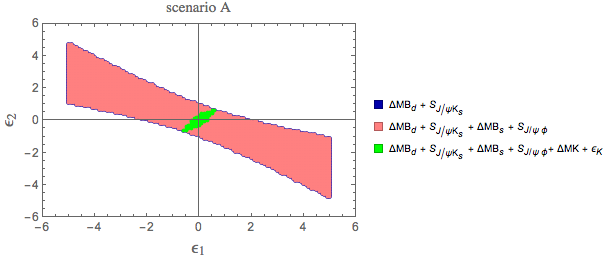
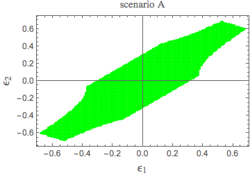
Refer to caption
Refer to caption
Figure 1: Scenario A. Left panel: Allowed region in the (ϵ𝟏,ϵ𝟐)subscriptbold-italic-ϵ1subscriptbold-italic-ϵ2(\epsilon_{1},\,\epsilon_{2}) plane, after imposing 𝚫𝑭=𝟐𝚫𝑭2\Delta F=2 constraints, as indicated in the legend. Right panel: Zoom of the green zone in the left panel.

The impact on the observables related to the 𝑩𝒅subscript𝑩𝒅B_{d} and 𝑩𝒔subscript𝑩𝒔B_{s} system is small. For example, we find that effects on 𝓑(𝑩𝒅𝝁+𝝁)𝓑bold-→subscript𝑩𝒅superscript𝝁superscript𝝁{\cal B}(B_{d}\to\mu^{+}\mu^{-}) and 𝓑¯(𝑩𝒔𝝁+𝝁)bold-¯𝓑bold-→subscript𝑩𝒔superscript𝝁superscript𝝁{\bar{\cal B}}(B_{s}\to\mu^{+}\mu^{-}) are at most 𝟐%percent22\% in this scenario, while effects on the Wilson coefficients 𝑪𝟗subscript𝑪9C_{9} and 𝑪𝟏𝟎subscript𝑪10C_{10} entering in the description of rare 𝒃𝒔bold-→𝒃𝒔b\to s decays are negligible. For this reason, we do not show the corresponding plots. As for Kaon decays, while effects on 𝑲𝑳𝝅𝟎𝝂𝝂¯bold-→subscript𝑲𝑳superscript𝝅0𝝂bold-¯𝝂K_{L}\to\pi^{0}\nu{\bar{\nu}} are tiny, significant deviations from the SM at the level of 𝟐𝟎%percent2020\% are still allowed for 𝑲+𝝅+𝝂𝝂¯bold-→superscript𝑲superscript𝝅𝝂bold-¯𝝂K^{+}\to\pi^{+}\nu\bar{\nu} by 𝚫𝑭=𝟐𝚫𝑭2\Delta F=2 constraints, as can be observed from Fig. 2. This scenario does not predict an enhancement of |𝜺/𝜺|superscript𝜺bold-′𝜺|\varepsilon^{\prime}/\varepsilon| with respect to the SM prediction: the largest deviation from the SM is 𝟐𝟏𝟎𝟓similar-to-or-equalsabsentbold-⋅2superscript105\simeq 2\cdot 10^{-5}, two orders of magnitude below its experimental value.
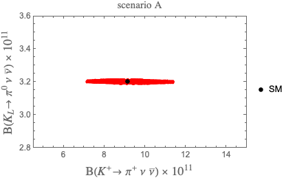
Refer to caption
Figure 2: Scenario A. Correlation between 𝓑(𝑲𝑳𝝅𝟎𝝂𝝂¯)𝓑bold-→subscript𝑲𝑳superscript𝝅0𝝂bold-¯𝝂{\cal B}(K_{L}\to\pi^{0}\nu{\bar{\nu}}) and 𝓑(𝑲+𝝅+𝝂𝝂¯)𝓑bold-→superscript𝑲superscript𝝅𝝂bold-¯𝝂{\cal B}(K^{+}\to\pi^{+}\nu\bar{\nu}). The black dot represents the central value of the SM prediction.
Refer to caption
Refer to caption
Figure 3: Scenario A. Correlation between 𝓑(𝝉𝝁𝝁+𝝁)𝓑bold-→superscript𝝉superscript𝝁superscript𝝁superscript𝝁{\cal B}(\tau^{-}\to\mu^{-}\mu^{+}\mu^{-}) and 𝓑(𝝉𝒆𝒆+𝒆)𝓑bold-→superscript𝝉superscript𝒆superscript𝒆superscript𝒆{\cal B}(\tau^{-}\to e^{-}e^{+}e^{-}) (left panel) and between 𝓑(𝝉𝝁𝝁+𝝁)𝓑bold-→superscript𝝉superscript𝝁superscript𝝁superscript𝝁{\cal B}(\tau^{-}\to\mu^{-}\mu^{+}\mu^{-}) and 𝓑(𝝁𝒆𝒆+𝒆)𝓑bold-→superscript𝝁superscript𝒆superscript𝒆superscript𝒆{\cal B}(\mu^{-}\to e^{-}e^{+}e^{-}) (right panel). The gray shaded region in the right panel is excluded by the experimental bound 𝓑(𝝁𝒆𝒆+𝒆)<𝟏𝟏𝟎𝟏𝟐𝓑bold-→superscript𝝁superscript𝒆superscript𝒆superscript𝒆bold-⋅1superscript1012{\cal B}(\mu^{-}\to e^{-}e^{+}e^{-})<1\cdot 10^{-12}.
Refer to caption
Refer to caption
Refer to caption
Figure 4: Scenario A. Correlation between 𝓑(𝑲+𝝅+𝝂𝝂¯)𝓑bold-→superscript𝑲superscript𝝅𝝂bold-¯𝝂{\cal B}(K^{+}\to\pi^{+}\nu\bar{\nu}) and 𝓑(𝝁𝒆𝒆+𝒆)𝓑bold-→superscript𝝁superscript𝒆superscript𝒆superscript𝒆{\cal B}(\mu^{-}\to e^{-}e^{+}e^{-}) (upper left panel) and between 𝓑(𝑲+𝝅+𝝂𝝂¯)𝓑bold-→superscript𝑲superscript𝝅𝝂bold-¯𝝂{\cal B}(K^{+}\to\pi^{+}\nu\bar{\nu}) and 𝓑(𝝁𝒆𝜸)𝓑bold-→superscript𝝁superscript𝒆𝜸{\cal B}(\mu^{-}\to e^{-}\gamma) (upper right panel). Correlation between 𝓑(𝝁𝒆𝜸)𝓑bold-→superscript𝝁superscript𝒆𝜸{\cal B}(\mu^{-}\to e^{-}\gamma) and 𝓑(𝝁𝒆𝒆+𝒆)𝓑bold-→superscript𝝁superscript𝒆superscript𝒆superscript𝒆{\cal B}(\mu^{-}\to e^{-}e^{+}e^{-}) (lower panel). The gray shaded regions are excluded by the experimental bound 𝓑(𝝁𝒆𝒆+𝒆)<𝟏𝟏𝟎𝟏𝟐𝓑bold-→superscript𝝁superscript𝒆superscript𝒆superscript𝒆bold-⋅1superscript1012{\cal B}(\mu^{-}\to e^{-}e^{+}e^{-})<1\cdot 10^{-12}.

Fig. 3 displays the results for flavour violating lepton decays. The left panel shows that 𝝉𝝉\tau decays are predicted well below the experimental upper bounds in (101)-(102). On the other hand, 𝓑(𝝁𝒆𝒆+𝒆)𝓑bold-→superscript𝝁superscript𝒆superscript𝒆superscript𝒆{\cal B}(\mu^{-}\to e^{-}e^{+}e^{-}) shown in the right panel can easily be close to the experimental bound (103) and even exceed it.

Also 𝓑(𝝁𝒆𝜸)𝓑bold-→superscript𝝁superscript𝒆𝜸{\cal B}(\mu^{-}\to e^{-}\gamma) is predicted below the bound in (97), as can be inferred from the upper right panel in Fig. 4. In this figure, we display the correlations among lepton decays 𝝁𝒆𝒆+𝒆bold-→superscript𝝁superscript𝒆superscript𝒆superscript𝒆\mu^{-}\to e^{-}e^{+}e^{-}, 𝝁𝒆𝜸bold-→superscript𝝁superscript𝒆𝜸\mu^{-}\to e^{-}\gamma and the mode 𝑲+𝝅+𝝂𝝂¯bold-→superscript𝑲superscript𝝅𝝂bold-¯𝝂K^{+}\to\pi^{+}\nu{\bar{\nu}}. The upper panels show, that in this scenario, the experimental bound on both leptonic decays have no impact on the possibility that 𝓑(𝑲+𝝅+𝝂𝝂¯)𝓑bold-→superscript𝑲superscript𝝅𝝂bold-¯𝝂{\cal B}(K^{+}\to\pi^{+}\nu{\bar{\nu}}) could significantly deviate from its SM value. On the other hand, the bound on 𝓑(𝝁𝒆𝒆+𝒆)𝓑bold-→superscript𝝁superscript𝒆superscript𝒆superscript𝒆{\cal B}(\mu^{-}\to e^{-}e^{+}e^{-}) reduces the allowed range for 𝓑(𝝁𝒆𝜸)𝓑bold-→superscript𝝁superscript𝒆𝜸{\cal B}(\mu^{-}\to e^{-}\gamma) (lower panel); however, this branching ratio is much smaller than the experimental upper bound, as already observed.

Comparing Fig. 5 with Fig. 2 we observe that the upper bound on 𝝁𝒆𝝁𝒆\mu-e conversion in the ballpark of 𝟏𝟎𝟏𝟐superscript101210^{-12} reduces significantly the allowed range for 𝓑(𝑲+𝝅+𝝂𝝂¯)𝓑bold-→superscript𝑲superscript𝝅𝝂bold-¯𝝂{\cal B}(K^{+}\to\pi^{+}\nu\bar{\nu}). On the other hand, as seen in this figure it has presently no impact on the allowed range for 𝝁𝒆𝒆+𝒆bold-→superscript𝝁superscript𝒆superscript𝒆superscript𝒆\mu^{-}\to e^{-}e^{+}e^{-}. This is also the case of 𝝁𝒆𝜸bold-→superscript𝝁superscript𝒆𝜸\mu^{-}\to e^{-}\gamma not shown here.

Refer to caption
Refer to caption
Figure 5: Scenario A. Correlation between 𝓑(𝝁𝐞)𝓑bold-→superscript𝝁superscript𝐞{\cal B}(\mu^{-}\to\mathrm{e}^{-}) and 𝓑(𝝁𝒆𝒆+𝒆)𝓑bold-→superscript𝝁superscript𝒆superscript𝒆superscript𝒆{\cal B}(\mu^{-}\to e^{-}e^{+}e^{-}) (left panel). The gray shaded region is excluded by the experimental bound 𝓑(𝝁𝒆𝒆+𝒆)<𝟏𝟏𝟎𝟏𝟐𝓑bold-→superscript𝝁superscript𝒆superscript𝒆superscript𝒆bold-⋅1superscript1012{\cal B}(\mu^{-}\to e^{-}e^{+}e^{-})<1\cdot 10^{-12}. Correlation between 𝓑(𝝁𝐞)𝓑bold-→superscript𝝁superscript𝐞{\cal B}(\mu^{-}\to\mathrm{e}^{-}) and 𝓑(𝑲+𝝅+𝝂𝝂¯)𝓑bold-→superscript𝑲superscript𝝅𝝂bold-¯𝝂{\cal B}(K^{+}\to\pi^{+}\nu\bar{\nu}) (right panel).

6.2 Results in Scenario B1

The result of the subsequent application of the constraints (112)-(114) is shown in the upper panel of Fig. 6.
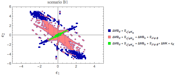
Refer to caption
Refer to caption
Figure 6: Scenarios B1 (upper panel) and B2 (lower panel). Allowed region in the (ϵ𝟏,ϵ𝟐)subscriptbold-italic-ϵ1subscriptbold-italic-ϵ2(\epsilon_{1},\,\epsilon_{2}) plane, after imposing 𝚫𝑭=𝟐𝚫𝑭2\Delta F=2 constraints, as indicated in the legend.
Refer to caption
Refer to caption
Figure 7: Scenarios B1 (left panel) and B2 (right panel). Correlation between 𝓑(𝑩𝒅𝝁+𝝁)𝓑bold-→subscript𝑩𝒅superscript𝝁superscript𝝁{\cal B}(B_{d}\to\mu^{+}\mu^{-}) and 𝓑¯(𝑩𝒔𝝁+𝝁)bold-¯𝓑bold-→subscript𝑩𝒔superscript𝝁superscript𝝁{\cal\bar{B}}(B_{s}\to\mu^{+}\mu^{-}). The black dot represents the central value of the SM prediction.
Refer to caption
Refer to caption
Figure 8: Scenarios B1 (upper plots) and B2 (lower plots). Wilson coefficients that appear in the 𝒃𝒔+bold-→𝒃𝒔superscriptbold-ℓsuperscriptbold-ℓb\to s\ell^{+}\ell^{-} effective Hamiltonian. Only those sensibly different from zero are displayed: 𝑪𝟗superscriptsubscript𝑪9bold-′C_{9}^{\prime} and 𝑪𝟏𝟎superscriptsubscript𝑪10bold-′C_{10}^{\prime} (not present in the SM) in scenario B1 (upper plots) and in B2 (lower middle and right plots). In the case of B2 deviation from the SM value of 𝐑𝐞[𝑪𝟗]𝐑𝐞delimited-[]subscript𝑪9{\rm Re}[C_{9}] and 𝐑𝐞[𝑪𝟏𝟎]𝐑𝐞delimited-[]subscript𝑪10{\rm Re}[C_{10}] are also shown (lower left plot).

At odds with the previous scenario, in this case one can have significant deviations from the SM predictions in 𝑩𝒅,𝒔subscript𝑩𝒅𝒔B_{d,s} observables. This is for instance the case for the rare decays 𝑩𝒅,𝒔𝝁+𝝁bold-→subscript𝑩𝒅𝒔superscript𝝁superscript𝝁B_{d,s}\to\mu^{+}\mu^{-}. As Fig. 7 (left panel) shows, the branching ratios of these modes can largely deviate from the SM results whose central values are represented by the black dot in that figure.

The most recent averages from the data of CMS, LHCb and ATLAS [53, 54, 55, 56] have been presented in [23] with the result

𝓑¯(𝑩𝒔𝝁+𝝁)=(2.71±0.40)×𝟏𝟎𝟗,𝓑(𝑩𝒅𝝁+𝝁)=(1.01±0.81)×𝟏𝟎𝟏𝟎.formulae-sequencebold-¯𝓑bold-→subscript𝑩𝒔superscript𝝁superscript𝝁plus-or-minus2.710.40superscript109𝓑bold-→subscript𝑩𝒅superscript𝝁superscript𝝁plus-or-minus1.010.81superscript1010\overline{\mathcal{B}}(B_{s}\to\mu^{+}\mu^{-})=(2.71\pm 0.40)\times 10^{-9},\qquad\mathcal{B}(B_{d}\to\mu^{+}\mu^{-})=(1.01\pm 0.81)\times 10^{-10}. (118)

In the case of 𝑩𝒔𝝁+𝝁bold-→subscript𝑩𝒔superscript𝝁superscript𝝁B_{s}\to\mu^{+}\mu^{-}, we observe a departure of the data from the SM prediction by about 𝟐𝝈2𝝈2\sigma. This favoures NP scenarios in which the branching ratio for this decay is suppressed relatively to its SM value [23]

𝓑¯(𝑩𝒔𝝁+𝝁)𝐒𝐌=(3.67±0.15)×𝟏𝟎𝟗,𝓑(𝑩𝒅𝝁+𝝁)=(1.14±0.12)×𝟏𝟎𝟏𝟎.formulae-sequencebold-¯𝓑subscriptbold-→subscript𝑩𝒔superscript𝝁superscript𝝁𝐒𝐌plus-or-minus3.670.15superscript109𝓑bold-→subscript𝑩𝒅superscript𝝁superscript𝝁plus-or-minus1.140.12superscript1010\overline{\mathcal{B}}(B_{s}\to\mu^{+}\mu^{-})_{\rm SM}=(3.67\pm 0.15)\times 10^{-9},\qquad\mathcal{B}(B_{d}\to\mu^{+}\mu^{-})=(1.14\pm 0.12)\times 10^{-10}. (119)

The relevant formulae for these observables when a new 𝒁superscript𝒁bold-′Z^{\prime} contribution is added can be found in Section 3 of [3], as well as, those of the Wilson coefficients of the 𝒃𝒔+bold-→𝒃𝒔superscriptbold-ℓsuperscriptbold-ℓb\to s\ell^{+}\ell^{-} effective Hamiltonian that we are going to consider. Among such coefficients 𝑪𝟗subscript𝑪9C_{9} and 𝑪𝟏𝟎subscript𝑪10C_{10} are already present in the SM, and we shall consider only the shift with respect to their SM values, denoted by 𝑪𝟗𝐍𝐏superscriptsubscript𝑪9𝐍𝐏C_{9}^{\rm NP} and 𝑪𝟏𝟎𝐍𝐏superscriptsubscript𝑪10𝐍𝐏C_{10}^{\rm NP}. 𝑪𝟗superscriptsubscript𝑪9bold-′C_{9}^{\prime} and 𝑪𝟏𝟎superscriptsubscript𝑪10bold-′C_{10}^{\prime} are instead absent in the SM, so these represent pure NP quantities. Various analyses have been devoted to fit the Wilson coefficients in order to explain the observed anomalies in a number of 𝒃𝒔bold-→𝒃𝒔b\to s related observables. Among the possible solutions, it has been pointed out that a large negative value of 𝑪𝟗𝐍𝐏superscriptsubscript𝑪9𝐍𝐏C_{9}^{\rm NP} or a large 𝑪𝟗superscriptsubscript𝑪9bold-′C_{9}^{\prime} could be effective. Our results for the various coefficients in scenario B1 are displayed in the upper panel of Fig. 8. Deviations from the SM are negligible for 𝑪𝟗𝐍𝐏superscriptsubscript𝑪9𝐍𝐏C_{9}^{\rm NP} and 𝑪𝟏𝟎𝐍𝐏superscriptsubscript𝑪10𝐍𝐏C_{10}^{\rm NP} but could be relevant in the case of 𝑪𝟗superscriptsubscript𝑪9bold-′C_{9}^{\prime} and 𝑪𝟏𝟎superscriptsubscript𝑪10bold-′C_{10}^{\prime} and we display only them.

In the Kaon sector, we find that 𝓑(𝑲𝑳𝝅𝟎𝝂𝝂¯)𝓑bold-→subscript𝑲𝑳superscript𝝅0𝝂bold-¯𝝂{\cal B}(K_{L}\to\pi^{0}\nu{\bar{\nu}}) displays small deviations from the SM, while 𝓑(𝑲+𝝅+𝝂𝝂¯)𝓑bold-→superscript𝑲superscript𝝅𝝂bold-¯𝝂{\cal B}(K^{+}\to\pi^{+}\nu{\bar{\nu}}) can be strongly enhanced or suppressed with respect to the SM result, when 𝓑(𝑲𝑳𝝅𝟎𝝂𝝂¯)𝓑bold-→subscript𝑲𝑳superscript𝝅0𝝂bold-¯𝝂{\cal B}(K_{L}\to\pi^{0}\nu{\bar{\nu}}) is SM-like, while it is approximately stable on the SM value when 𝓑(𝑲𝑳𝝅𝟎𝝂𝝂¯)𝓑bold-→subscript𝑲𝑳superscript𝝅0𝝂bold-¯𝝂{\cal B}(K_{L}\to\pi^{0}\nu{\bar{\nu}}) deviates from the SM central value. This pattern of correlation is shown in the left panel of Fig. 9.

As for scenario A, also in B1 lepton flavour violating 𝝉𝝉\tau decays are predicted below the experimental upper limit, while 𝓑(𝝁𝒆𝒆+𝒆)𝓑bold-→superscript𝝁superscript𝒆superscript𝒆superscript𝒆{\cal B}(\mu^{-}\to e^{-}e^{+}e^{-}) can saturate or even exceed its experimental upper bound. Correlations among these modes are displayed in the upper panel of Fig. 10.

In contrast to the case of scenario A, in B1 𝓑(𝝁𝒆𝜸)𝓑bold-→superscript𝝁superscript𝒆𝜸{\cal B}(\mu^{-}\to e^{-}\gamma) can saturate or even exceed the experimental upper bound. Correlations among the lepton observables 𝓑(𝝁𝒆𝒆+𝒆)𝓑bold-→superscript𝝁superscript𝒆superscript𝒆superscript𝒆{\cal B}(\mu^{-}\to e^{-}e^{+}e^{-}) or 𝓑(𝝁𝒆𝜸)𝓑bold-→superscript𝝁superscript𝒆𝜸{\cal B}(\mu^{-}\to e^{-}\gamma) and 𝓑(𝑲+𝝅+𝝂𝝂¯)𝓑bold-→superscript𝑲superscript𝝅𝝂bold-¯𝝂{\cal B}(K^{+}\to\pi^{+}\nu\bar{\nu}) are shown in Fig. 11 (upper plots). The experimental bound on 𝓑(𝝁𝒆𝜸)𝓑bold-→superscript𝝁superscript𝒆𝜸{\cal B}(\mu^{-}\to e^{-}\gamma) has no impact on the 𝑲+superscript𝑲K^{+} branching ratio. However, one can observe that, the bound on 𝓑(𝝁𝒆𝒆+𝒆)𝓑bold-→superscript𝝁superscript𝒆superscript𝒆superscript𝒆{\cal B}(\mu^{-}\to e^{-}e^{+}e^{-}) allows only the values for 𝓑(𝑲+𝝅+𝝂𝝂¯)𝓑bold-→superscript𝑲superscript𝝅𝝂bold-¯𝝂{\cal B}(K^{+}\to\pi^{+}\nu\bar{\nu}) close to its SM value.

The situation is different when one considers the ratio 𝜺/𝜺superscript𝜺bold-′𝜺\varepsilon^{\prime}/\varepsilon and, in particular, its deviation from the SM. As the upper left panel of Fig. 12 shows, in B1 |(𝜺/𝜺)𝐁𝐒𝐌|subscriptsuperscript𝜺bold-′𝜺𝐁𝐒𝐌|\left(\varepsilon^{\prime}/\varepsilon\right)_{\rm BSM}| could reach values as large as 1.5𝟏𝟎𝟒similar-to-or-equalsabsentbold-⋅1.5superscript104\simeq 1.5\cdot 10^{-4}. However, imposing that 𝓑(𝝁𝒆𝜸)𝓑bold-→superscript𝝁superscript𝒆𝜸{\cal B}(\mu^{-}\to e^{-}\gamma) lies below its experimental upper limit, one finds that the maximum deviation in 𝜺/𝜺superscript𝜺bold-′𝜺\varepsilon^{\prime}/\varepsilon could be |(𝜺/𝜺)𝐁𝐒𝐌|0.6𝟏𝟎𝟒similar-to-or-equalssubscriptsuperscript𝜺bold-′𝜺𝐁𝐒𝐌bold-⋅0.6superscript104|\left(\varepsilon^{\prime}/\varepsilon\right)_{\rm BSM}|\simeq 0.6\cdot 10^{-4}. As for the correlation between (𝜺/𝜺)𝐁𝐒𝐌subscriptsuperscript𝜺bold-′𝜺𝐁𝐒𝐌\left(\varepsilon^{\prime}/\varepsilon\right)_{\rm BSM} and 𝓑(𝑲+𝝅+𝝂𝝂¯)𝓑bold-→superscript𝑲superscript𝝅𝝂bold-¯𝝂{\cal B}(K^{+}\to\pi^{+}\nu\bar{\nu}), from the right upper panel of Fig. 12 one can observe that deviations in one of the two observables with respect to the SM predictions exclude deviations in the other one.

But what is most important is the impact of the bounds on leptonic modes on rare 𝑩𝑩B and 𝑲𝑲K decay branching ratios seen already in the case of Scenario A. First one can observe from the upper plots in Fig. 13 that, even if in B1 𝓑¯(𝑩𝒔𝝁+𝝁)bold-¯𝓑bold-→subscript𝑩𝒔superscript𝝁superscript𝝁{\cal\bar{B}}(B_{s}\to\mu^{+}\mu^{-}) can deviate significantly from its SM value, constraints in the lepton sector reduce the size of such a deviation. This is in particular the case when the bound from 𝝁𝒆𝒆+𝒆bold-→superscript𝝁superscript𝒆superscript𝒆superscript𝒆\mu^{-}\to e^{-}e^{+}e^{-} is applied.

But even stronger impact comes from 𝝁𝒆𝝁𝒆\mu-e conversion. Indeed comparing Fig. 14 with Figs. 7 and 9 we observe that the upper bound on 𝝁𝒆𝝁𝒆\mu-e conversion in the ballpark of 𝟏𝟎𝟏𝟐superscript101210^{-12} reduces significantly the allowed ranges for 𝑩𝒔𝝁+𝝁bold-→subscript𝑩𝒔superscript𝝁superscript𝝁B_{s}\to\mu^{+}\mu^{-} and 𝑲+𝝅+𝝂𝝂¯bold-→superscript𝑲superscript𝝅𝝂bold-¯𝝂K^{+}\to\pi^{+}\nu\bar{\nu} branching ratios. On the other hand, as seen in other plots it has presently no impact on the allowed ranges for 𝝁𝒆𝒆+𝒆bold-→superscript𝝁superscript𝒆superscript𝒆superscript𝒆\mu^{-}\to e^{-}e^{+}e^{-} and 𝝁𝒆𝜸bold-→superscript𝝁superscript𝒆𝜸\mu^{-}\to e^{-}\gamma.

Scenario B1, similar to Scenario A shows a peculiar feature that often occurs in our model: in principle large deviations from SM predictions can be found. However, quark and lepton sector act in a complementary way to constrain each other producing observables with values close to the SM ones.
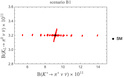
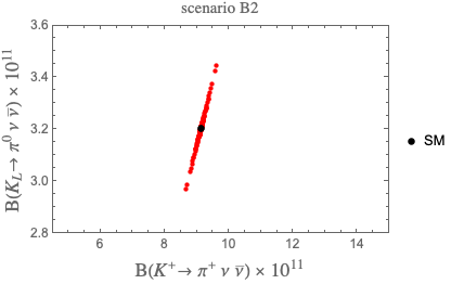
Refer to caption
Refer to caption
Figure 9: Scenarios B1 (left panel) and B2 (right panel). Correlation between 𝓑(𝑲𝑳𝝅𝟎𝝂𝝂¯)𝓑bold-→subscript𝑲𝑳superscript𝝅0𝝂bold-¯𝝂{\cal B}(K_{L}\to\pi^{0}\nu{\bar{\nu}}) and 𝓑(𝑲+𝝅+𝝂𝝂¯)𝓑bold-→superscript𝑲superscript𝝅𝝂bold-¯𝝂{\cal B}(K^{+}\to\pi^{+}\nu\bar{\nu}). The black dot represents the central value of the SM prediction.
Refer to caption
Refer to caption
Refer to caption
Refer to caption
Figure 10: Scenarios B1 (upper plots) and B2 (lower plots). Correlation between 𝓑(𝝉𝝁𝝁+𝝁)𝓑bold-→superscript𝝉superscript𝝁superscript𝝁superscript𝝁{\cal B}(\tau^{-}\to\mu^{-}\mu^{+}\mu^{-}) and 𝓑(𝝉𝒆𝒆+𝒆)𝓑bold-→superscript𝝉superscript𝒆superscript𝒆superscript𝒆{\cal B}(\tau^{-}\to e^{-}e^{+}e^{-}) (left panel) and between 𝓑(𝝉𝝁𝝁+𝝁)𝓑bold-→superscript𝝉superscript𝝁superscript𝝁superscript𝝁{\cal B}(\tau^{-}\to\mu^{-}\mu^{+}\mu^{-}) and 𝓑(𝝁𝒆𝒆+𝒆)𝓑bold-→superscript𝝁superscript𝒆superscript𝒆superscript𝒆{\cal B}(\mu^{-}\to e^{-}e^{+}e^{-}) (right panel). The gray shaded region in the right panel is excluded by the experimental bound 𝓑(𝝁𝒆𝒆+𝒆)<𝟏𝟏𝟎𝟏𝟐𝓑bold-→superscript𝝁superscript𝒆superscript𝒆superscript𝒆bold-⋅1superscript1012{\cal B}(\mu^{-}\to e^{-}e^{+}e^{-})<1\cdot 10^{-12}.
Refer to caption
Refer to caption
Refer to caption
Refer to caption
Figure 11: Scenarios B1 (upper plots) and B2 (lower plots). Correlation between 𝓑(𝑲+𝝅+𝝂𝝂¯)𝓑bold-→superscript𝑲superscript𝝅𝝂bold-¯𝝂{\cal B}(K^{+}\to\pi^{+}\nu\bar{\nu}) and 𝓑(𝝁𝒆𝒆+𝒆)𝓑bold-→superscript𝝁superscript𝒆superscript𝒆superscript𝒆{\cal B}(\mu^{-}\to e^{-}e^{+}e^{-}) (left panels) and between 𝓑(𝑲+𝝅+𝝂𝝂¯)𝓑bold-→superscript𝑲superscript𝝅𝝂bold-¯𝝂{\cal B}(K^{+}\to\pi^{+}\nu\bar{\nu}) and 𝓑(𝝁𝒆𝜸)𝓑bold-→superscript𝝁superscript𝒆𝜸{\cal B}(\mu^{-}\to e^{-}\gamma) (right panels). The gray shaded regions are excluded by the experimental bounds 𝓑(𝝁𝒆𝒆+𝒆)<𝟏𝟏𝟎𝟏𝟐𝓑bold-→superscript𝝁superscript𝒆superscript𝒆superscript𝒆bold-⋅1superscript1012{\cal B}(\mu^{-}\to e^{-}e^{+}e^{-})<1\cdot 10^{-12} and 𝓑(𝝁𝒆𝜸)<4.2𝟏𝟎𝟏𝟑𝓑bold-→superscript𝝁superscript𝒆𝜸bold-⋅4.2superscript1013{\cal B}(\mu^{-}\to e^{-}\gamma)<4.2\cdot 10^{-13}.
Refer to caption
Refer to caption
Refer to caption
Refer to caption
Figure 12: Scenarios B1 (upper plots) and B2 (lower plots). Correlations involving the (𝜺/𝜺)𝐁𝐒𝐌subscriptsuperscript𝜺bold-′𝜺𝐁𝐒𝐌\left(\varepsilon^{\prime}/\varepsilon\right)_{\rm BSM} (the NP contribution to 𝜺/𝜺superscript𝜺bold-′𝜺\varepsilon^{\prime}/\varepsilon). Correlation with 𝓑(𝝁𝒆𝜸)𝓑bold-→superscript𝝁superscript𝒆𝜸{\cal B}(\mu^{-}\to e^{-}\gamma) (left panels) and with 𝓑(𝑲+𝝅+𝝂𝝂¯)𝓑bold-→superscript𝑲superscript𝝅𝝂bold-¯𝝂{\cal B}(K^{+}\to\pi^{+}\nu\bar{\nu}) (right panels). The gray shaded region is excluded by the experimental bound 𝓑(𝝁𝒆𝜸)<4.2𝟏𝟎𝟏𝟑𝓑bold-→superscript𝝁superscript𝒆𝜸bold-⋅4.2superscript1013{\cal B}(\mu^{-}\to e^{-}\gamma)<4.2\cdot 10^{-13}.
Refer to caption
Refer to caption
Refer to caption
Refer to caption
Figure 13: Scenarios B1 (upper plots) and B2 (lower plots). Correlations between 𝓑¯(𝑩𝒔𝝁+𝝁)bold-¯𝓑bold-→subscript𝑩𝒔superscript𝝁superscript𝝁{\cal\bar{B}}(B_{s}\to\mu^{+}\mu^{-}) and 𝓑(𝝁𝒆𝒆+𝒆)𝓑bold-→superscript𝝁superscript𝒆superscript𝒆superscript𝒆{\cal B}(\mu^{-}\to e^{-}e^{+}e^{-}) (left panels) and between 𝓑¯(𝑩𝒔𝝁+𝝁)bold-¯𝓑bold-→subscript𝑩𝒔superscript𝝁superscript𝝁{\cal\bar{B}}(B_{s}\to\mu^{+}\mu^{-}) and 𝓑(𝝁𝒆𝜸)𝓑bold-→superscript𝝁superscript𝒆𝜸{\cal B}(\mu^{-}\to e^{-}\gamma) (right panels). The gray shaded regions are excluded by the experimental bounds 𝓑(𝝁𝒆𝒆+𝒆)<𝟏𝟏𝟎𝟏𝟐𝓑bold-→superscript𝝁superscript𝒆superscript𝒆superscript𝒆bold-⋅1superscript1012{\cal B}(\mu^{-}\to e^{-}e^{+}e^{-})<1\cdot 10^{-12} and 𝓑(𝝁𝒆𝜸)<4.2𝟏𝟎𝟏𝟑𝓑bold-→superscript𝝁superscript𝒆𝜸bold-⋅4.2superscript1013{\cal B}(\mu^{-}\to e^{-}\gamma)<4.2\cdot 10^{-13}.
Refer to caption
Refer to caption
Refer to caption
Refer to caption
Refer to caption
Refer to caption
Figure 14: Scenarios B1 (upper plots) and B2 (lower plots). Correlation between 𝓑(𝝁𝐞)𝓑bold-→superscript𝝁superscript𝐞{\cal B}(\mu^{-}\to\mathrm{e}^{-}) and 𝓑(𝝁𝒆𝒆+𝒆)𝓑bold-→superscript𝝁superscript𝒆superscript𝒆superscript𝒆{\cal B}(\mu^{-}\to e^{-}e^{+}e^{-}) (left panels). The gray shaded region is excluded by the experimental bound 𝓑(𝝁𝒆𝒆+𝒆)<𝟏𝟏𝟎𝟏𝟐𝓑bold-→superscript𝝁superscript𝒆superscript𝒆superscript𝒆bold-⋅1superscript1012{\cal B}(\mu^{-}\to e^{-}e^{+}e^{-})<1\cdot 10^{-12}. Correlations between 𝓑(𝝁𝐞)𝓑bold-→superscript𝝁superscript𝐞{\cal B}(\mu^{-}\to\mathrm{e}^{-}) and 𝓑¯(𝑩𝒔𝝁+𝝁)bold-¯𝓑bold-→subscript𝑩𝒔superscript𝝁superscript𝝁{\cal\bar{B}}(B_{s}\to\mu^{+}\mu^{-}) (middle panels) and between 𝓑(𝝁𝐞)𝓑bold-→superscript𝝁superscript𝐞{\cal B}(\mu^{-}\to\mathrm{e}^{-}) and 𝓑(𝑲+𝝅+𝝂𝝂¯)𝓑bold-→superscript𝑲superscript𝝅𝝂bold-¯𝝂{\cal B}(K^{+}\to\pi^{+}\nu\bar{\nu}) (right panels).

6.3 Results in Scenario B2

The parameter space in B2 is simplified because of the assumption ϵ𝟏=ϵ𝟐subscriptbold-italic-ϵ1subscriptbold-italic-ϵ2\epsilon_{1}=\epsilon_{2}, as can be observed from the lower panel in Fig. 6. As in the case of B1, also B2 displays large deviations from the SM in the 𝑩𝒅,𝒔subscript𝑩𝒅𝒔B_{d,s} sectors. Fig. 7 (right panel) shows that the rare decays 𝓑(𝑩𝒅𝝁+𝝁)𝓑bold-→subscript𝑩𝒅superscript𝝁superscript𝝁{\cal B}(B_{d}\to\mu^{+}\mu^{-}) and 𝓑¯(𝑩𝒔𝝁+𝝁)bold-¯𝓑bold-→subscript𝑩𝒔superscript𝝁superscript𝝁{\cal\bar{B}}(B_{s}\to\mu^{+}\mu^{-}) are approximately linearly correlated, and can strongly deviate from the SM. As for the Wilson coefficients 𝑪𝟗(),𝑪𝟏𝟎()superscriptsubscript𝑪9superscriptsubscript𝑪10C_{9}^{(\prime)},\,C_{10}^{(\prime)}, in B2 one finds that 𝐈𝐦(𝐂𝟗)𝟎similar-to-or-equals𝐈𝐦subscript𝐂90\rm{Im}(C_{9})\simeq 0 and 𝐈𝐦(𝐂𝟏𝟎)𝟎similar-to-or-equals𝐈𝐦subscript𝐂100\rm{Im}(C_{10})\simeq 0, deviations in 𝐑𝐞(𝐂𝟗)𝐑𝐞subscript𝐂9\rm{Re}(C_{9}) and 𝐑𝐞(𝐂𝟏𝟎)𝐑𝐞subscript𝐂10\rm{Re}(C_{10}) are of the same size as in B1, while 𝑪𝟗,𝑪𝟏𝟎superscriptsubscript𝑪9bold-′superscriptsubscript𝑪10bold-′C_{9}^{\prime},\,C_{10}^{\prime} vary in much larger ranges, as can be seen in Fig. 8 (lower plots). However, if the experimental bound on 𝓑(𝝁𝒆𝒆+𝒆)𝓑bold-→superscript𝝁superscript𝒆superscript𝒆superscript𝒆{\cal B}(\mu^{-}\to e^{-}e^{+}e^{-}) is imposed, these variations are practically removed as indicated by the central blue regions in Fig. 8. This is another example of the mutual role of lepton and quark sectors.

Looking at rare Kaon decays, it can be observed that for ϵ𝟏=ϵ𝟐subscriptbold-italic-ϵ1subscriptbold-italic-ϵ2\epsilon_{1}=\epsilon_{2} the relation between 𝓑(𝑲𝑳𝝅𝟎𝝂𝝂¯)𝓑bold-→subscript𝑲𝑳superscript𝝅0𝝂bold-¯𝝂{\cal B}(K_{L}\to\pi^{0}\nu{\bar{\nu}}) and 𝓑(𝑲+𝝅+𝝂𝝂¯)𝓑bold-→superscript𝑲superscript𝝅𝝂bold-¯𝝂{\cal B}(K^{+}\to\pi^{+}\nu\bar{\nu}) is approximately linear. This result is displayed in the right plot in Fig. 9, which in addition shows that moderate variations with respect to the SM values are possible.

As in B1, among lepton decays the branching fractions that can be large are 𝓑(𝝁𝒆𝒆+𝒆)𝓑bold-→superscript𝝁superscript𝒆superscript𝒆superscript𝒆{\cal B}(\mu^{-}\to e^{-}e^{+}e^{-}), as shown by the lower plots in Fig. 10, and 𝓑(𝝁𝒆𝜸)𝓑bold-→superscript𝝁superscript𝒆𝜸{\cal B}(\mu^{-}\to e^{-}\gamma) (see lower plots in Fig. 11). Both reduce the possible range of 𝓑(𝑲+𝝅+𝝂𝝂¯)𝓑bold-→superscript𝑲superscript𝝅𝝂bold-¯𝝂{\cal B}(K^{+}\to\pi^{+}\nu\bar{\nu}), as shown in Fig. 11. They also reduce the range for (𝜺/𝜺)𝐁𝐒𝐌subscriptsuperscript𝜺bold-′𝜺𝐁𝐒𝐌\left(\varepsilon^{\prime}/\varepsilon\right)_{\rm BSM}, the impact of 𝓑(𝝁𝒆𝒆+𝒆)𝓑bold-→superscript𝝁superscript𝒆superscript𝒆superscript𝒆{\cal B}(\mu^{-}\to e^{-}e^{+}e^{-}) being much more constraining than that of 𝓑(𝝁𝒆𝜸)𝓑bold-→superscript𝝁superscript𝒆𝜸{\cal B}(\mu^{-}\to e^{-}\gamma), as shown in the lower left panel of Fig. 12. In B2 deviations from the SM are possible in both 𝜺/𝜺superscript𝜺bold-′𝜺\varepsilon^{\prime}/\varepsilon and 𝓑(𝑲+𝝅+𝝂𝝂¯)𝓑bold-→superscript𝑲superscript𝝅𝝂bold-¯𝝂{\cal B}(K^{+}\to\pi^{+}\nu\bar{\nu}) and the correlation between these two observables is shown in the right lower panel of Fig. 12.

Correlations between lepton decays and 𝓑¯(𝑩𝒔𝝁+𝝁)bold-¯𝓑bold-→subscript𝑩𝒔superscript𝝁superscript𝝁{\cal\bar{B}}(B_{s}\to\mu^{+}\mu^{-}), shown in Fig. 13, follow a pattern similar to that in B1.

In Fig. 15 we show that in this scenario NP effects in 𝜺/𝜺superscript𝜺bold-′𝜺\varepsilon^{\prime}/\varepsilon can be significant without having any impact on 𝒂𝝁,𝒆subscript𝒂𝝁𝒆a_{\mu,e}. Generally the contributions of NP to 𝒂𝝁,𝒆subscript𝒂𝝁𝒆a_{\mu,e} are very small in all scenarios considered and this is the only figure displaying them that we show.

Similar to Scenario B1, as seen in Fig. 14, the upper bound on 𝝁𝒆𝝁𝒆\mu-e conversion also in this scenario has a very large impact on 𝑲+𝝅+𝝂𝝂¯bold-→superscript𝑲superscript𝝅𝝂bold-¯𝝂K^{+}\rightarrow\pi^{+}\nu\bar{\nu} and 𝑩𝒔𝝁+𝝁bold-→subscript𝑩𝒔superscript𝝁superscript𝝁B_{s}\to\mu^{+}\mu^{-}.

Refer to caption
Refer to caption
Figure 15: Scenario B2. Correlation between NP contributions to 𝜺/𝜺superscript𝜺bold-′𝜺\varepsilon^{\prime}/\varepsilon and 𝒂𝒆subscript𝒂𝒆a_{e} (left plot) and 𝒂𝝁subscript𝒂𝝁a_{\mu} (right plot).

6.4 Results in Scenario C

Removing the 𝚫𝑭=𝟐𝚫𝑭2\Delta F=2 constraints using the arguments presented in the Appendix A makes NP effects much larger than in other scenarios. In this case very large NP effects in all 𝚫𝑭=𝟏𝚫𝑭1\Delta F=1 observables are possible so that hinted anomalies in various rare decays of mesons can easily be explained in the absence of pure leptonic decays. One example is shown in Fig. 16, where the branching ratios for 𝑩𝒔,𝒅𝝁+𝝁bold-→subscript𝑩𝒔𝒅superscript𝝁superscript𝝁B_{s,d}\to\mu^{+}\mu^{-} decays are much more modified than in previous scenarios. Another example is shown in Fig. 17, where NP effects in 𝑲+𝝅+𝝂𝝂¯bold-→superscript𝑲superscript𝝅𝝂bold-¯𝝂K^{+}\rightarrow\pi^{+}\nu\bar{\nu} and 𝑲𝑳𝝅𝟎𝝂𝝂¯bold-→subscript𝑲𝑳superscript𝝅0𝝂bold-¯𝝂K_{L}\rightarrow\pi^{0}\nu\bar{\nu} can be very large. It is also evident that without the 𝑲𝑳𝝁+𝝁bold-→subscript𝑲𝑳superscript𝝁superscript𝝁K_{L}\to\mu^{+}\mu^{-} constraint NP effects would be even larger.

Yet, when the bound from 𝝁𝒆𝝁𝒆\mu-e conversion is taken into account the imposition of the cancellation of gauge anomalies with the help of leptons has an important impact on the allowed values of various observables in the Kaon and 𝑩𝒔,𝒅subscript𝑩𝒔𝒅B_{s,d} systems. Indeed the experimental bound on 𝝁𝒆𝝁𝒆\mu-e conversion eliminates any significant departures from the SM expectations for 𝑲+𝝅+𝝂𝝂¯bold-→superscript𝑲superscript𝝅𝝂bold-¯𝝂K^{+}\rightarrow\pi^{+}\nu\bar{\nu} and 𝑩𝒔,𝒅𝝁+𝝁bold-→subscript𝑩𝒔𝒅superscript𝝁superscript𝝁B_{s,d}\to\mu^{+}\mu^{-}. We show this in Fig. 18. Similar comments apply to other observables.
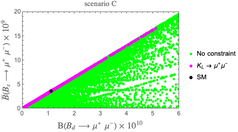
Refer to caption
Figure 16: Scenario C. Correlation between 𝓑(𝑩𝒅𝝁+𝝁)𝓑bold-→subscript𝑩𝒅superscript𝝁superscript𝝁{\cal B}(B_{d}\to\mu^{+}\mu^{-}) and 𝓑¯(𝑩𝒔𝝁+𝝁)bold-¯𝓑bold-→subscript𝑩𝒔superscript𝝁superscript𝝁{\cal\bar{B}}(B_{s}\to\mu^{+}\mu^{-}). The black dot represents the central value of the SM prediction.
Refer to caption
Figure 17: Scenario C. Correlation between 𝓑(𝑲𝑳𝝅𝟎𝝂𝝂¯)𝓑bold-→subscript𝑲𝑳superscript𝝅0𝝂bold-¯𝝂{\cal B}(K_{L}\to\pi^{0}\nu{\bar{\nu}}) and 𝓑(𝑲+𝝅+𝝂𝝂¯)𝓑bold-→superscript𝑲superscript𝝅𝝂bold-¯𝝂{\cal B}(K^{+}\to\pi^{+}\nu\bar{\nu}). The black dot represents the central value of the SM prediction.
Refer to caption
Refer to caption
Figure 18: Scenario C. Correlations between 𝓑(𝝁𝐞)𝓑bold-→superscript𝝁superscript𝐞{\cal B}(\mu^{-}\to\mathrm{e}^{-}) and 𝓑¯(𝑩𝒔𝝁+𝝁)bold-¯𝓑bold-→subscript𝑩𝒔superscript𝝁superscript𝝁{\cal\bar{B}}(B_{s}\to\mu^{+}\mu^{-}) (left panel) and between 𝓑(𝝁𝐞)𝓑bold-→superscript𝝁superscript𝐞{\cal B}(\mu^{-}\to\mathrm{e}^{-}) and 𝓑(𝑲+𝝅+𝝂𝝂¯)𝓑bold-→superscript𝑲superscript𝝅𝝂bold-¯𝝂{\cal B}(K^{+}\to\pi^{+}\nu\bar{\nu}) (right panel).

7 Conclusions

We have presented a simple extension of the SM based on the introduction of a new U(1) gauge group. We have fulfilled the requirement of anomaly cancellation in a rather special way, defining the charges under the new group in terms of three new parameters ϵ𝒊,𝒊=𝟏,𝟐,𝟑formulae-sequencesubscriptbold-italic-ϵ𝒊𝒊123\epsilon_{i},\,i=1,2,3 that are constrained to sum to zero, leaving only two as free parameters. Each of the three parameters governs one of the three fermion generations, so that quark and lepton sectors are connected to each other as far as their behaviour under the new gauge group is concerned. This leads to a constrained phenomenological panorama in which quark and lepton observables are correlated with each other. Independently of the structure of the 𝒁superscript𝒁bold-′Z^{\prime} couplings to fermions, that we have varied considering a few scenarios, we have found that imposing bounds from experimental data relative to 𝚫𝑭=𝟐𝚫𝑭2\Delta F=2 processes to constrain quark favour observables is not enough to prevent large deviations of these from their SM values. However, when constraints on lepton decays are imposed, the room for deviations is much reduced. In practice, quark and lepton sectors act simultaneously to produce a phenomenology similar to the SM. This can be a challenge to experiment but also shows that the pattern of data that we have at our disposal confirms the SM but does not exclude other scenarios like the one we are presenting.

We have also presented a scenario, following [57], in which a suitable hierarchy between LH and RH flavour violating couplings allows to remove the 𝚫𝑭=𝟐𝚫𝑭2\Delta F=2 constraints. In this case, as illustrated in a number of plots in Section 6.4, very large NP effects in all 𝚫𝑭=𝟏𝚫𝑭1\Delta F=1 observables can be obtained so that possible anomalies in various rare decays of mesons can easily be explained in the absence of pure leptonic decays. Yet as discussed on the examples of 𝑲+𝝅+𝝂𝝂¯bold-→superscript𝑲superscript𝝅𝝂bold-¯𝝂K^{+}\rightarrow\pi^{+}\nu\bar{\nu} and 𝑩𝒔,𝒅𝝁+𝝁bold-→subscript𝑩𝒔𝒅superscript𝝁superscript𝝁B_{s,d}\to\mu^{+}\mu^{-} even in this case the imposition of the cancellation of gauge anomalies with the help of leptons has an important impact on the allowed values of their branching ratios. This is in particular the case of the experimental bound on 𝝁𝒆𝝁𝒆\mu-e conversion that eliminates any significant departures from the SM expectations of 𝑩𝒔,𝒅𝝁+𝝁bold-→subscript𝑩𝒔𝒅superscript𝝁superscript𝝁B_{s,d}\to\mu^{+}\mu^{-} and 𝑲+𝝅+𝝂𝝂¯bold-→superscript𝑲superscript𝝅𝝂bold-¯𝝂K^{+}\rightarrow\pi^{+}\nu\bar{\nu} branching ratios as seen in Fig. 18.

The main lessons from our paper are the following ones:

  • In models in which the gauge anomalies in the quark sector are cancelled by the corresponding anomalies in the lepton sector the impact of the present experimental bounds on leptonic processes, such as 𝝁𝒆𝜸bold-→𝝁𝒆𝜸\mu\to e\gamma, 𝝁𝒆𝒆+𝒆bold-→𝝁superscript𝒆superscript𝒆superscript𝒆\mu\to e^{-}e^{+}e^{-} and in particular 𝝁𝒆𝝁𝒆\mu-e conversion can be very large unless the model has more free parameters than the simple models considered by us.

  • It appears then that a strategy for obtaining large NP effects while satisfying gauge anomaly cancellations is to construct models in which quark and lepton sectors are separately anomaly free.

Acknowledgements

We thank Robert Szafron for useful discussions. J.A. acknowledges financial support from the Swiss National Science Foundation (Project No. P400P2183838). The research of A.J.B and M. C-S was supported by the Excellence Cluster ORIGINS, funded by the Deutsche Forschungsgemeinschaft (DFG, German Research Foundation) under Germany’s Excellence Strategy – EXC-2094 – 390783311. The research of F.D.F. has been carried out within the INFN project (Iniziativa Specifica) QFT-HEP.

Appendix A Removing 𝚫𝑭=𝟐𝚫𝑭2\Delta F=2 Constraints

In the presence of both LH and RH couplings of a 𝒁superscript𝒁bold-′Z^{\prime} gauge boson to SM quarks left-right (LR) 𝚫𝑭=𝟐𝚫𝑭2\Delta F=2 operators are generated whose contributions to the mixing amplitudes 𝑴𝟏𝟐𝒃𝒒superscriptsubscript𝑴12𝒃𝒒M_{12}^{bq} and 𝑴𝟏𝟐𝒔𝒅superscriptsubscript𝑴12𝒔𝒅M_{12}^{sd} in all three mesonic systems are enhanced through renormalisation group effects relative to left-left (VLL) and right-right (VRR) operators. Moreover in the case of 𝑴𝟏𝟐𝒔𝒅superscriptsubscript𝑴12𝒔𝒅M_{12}^{sd} additional chiral enhancements of the hadronic matrix elements of LR operators are present. As pointed out in [57] this fact can be used to suppress NP contributions to 𝜺𝑲subscript𝜺𝑲\varepsilon_{K} and 𝚫𝑴𝑲𝚫subscript𝑴𝑲\Delta M_{K} through some fine-tuning between VLL, VRR and LR contributions, thereby allowing for larger contributions to 𝑲𝝅𝝅bold-→𝑲𝝅𝝅K\to\pi\pi amplitudes while satisfying the 𝚫𝑺=𝟐𝚫𝑺2\Delta S=2 constraints. In [58] this idea has been generalized to all three meson systems. While the fine-tuning required in the case of 𝑲𝝅𝝅bold-→𝑲𝝅𝝅K\to\pi\pi turned out to be rather large, it is more modest in case of 𝚫𝑩=𝟐𝚫𝑩2\Delta B=2 transitions.

We repeat here briefly the arguments presented in [57, 58]. Further details can be found in these two papers.

To this end we write the 𝒁superscript𝒁bold-′Z^{\prime} contributions to the mixing amplitudes as follows [3]:

(𝑴𝟏𝟐)𝒁𝒔𝒅=(𝚫𝑳𝒔𝒅)𝟐𝟐𝑴𝒁𝟐𝑸^𝟏VLL(𝑴𝒁)𝒔𝒅𝒛𝒔𝒅,superscriptsubscriptsuperscriptsubscript𝑴12superscript𝒁bold-′𝒔𝒅superscriptsuperscriptsubscript𝚫𝑳𝒔𝒅22superscriptsubscript𝑴superscript𝒁bold-′2superscriptdelimited-⟨⟩superscriptsubscriptbold-^𝑸1VLLsubscript𝑴superscript𝒁bold-′𝒔𝒅subscript𝒛𝒔𝒅(M_{12}^{*})_{Z^{\prime}}^{sd}=\frac{(\Delta_{L}^{sd})^{2}}{2M_{Z^{\prime}}^{2}}\langle\hat{Q}_{1}^{\text{VLL}}(M_{Z^{\prime}})\rangle^{sd}z_{sd}\,, (120)

and

(𝑴𝟏𝟐)𝒁𝒃𝒒=(𝚫𝑳𝒃𝒒)𝟐𝟐𝑴𝒁𝟐𝑸^𝟏VLL(𝑴𝒁)𝒃𝒒𝒛𝒃𝒒,superscriptsubscriptsuperscriptsubscript𝑴12superscript𝒁bold-′𝒃𝒒superscriptsuperscriptsubscript𝚫𝑳𝒃𝒒22superscriptsubscript𝑴superscript𝒁bold-′2superscriptdelimited-⟨⟩superscriptsubscriptbold-^𝑸1VLLsubscript𝑴superscript𝒁bold-′𝒃𝒒subscript𝒛𝒃𝒒(M_{12}^{*})_{Z^{\prime}}^{bq}=\frac{(\Delta_{L}^{bq})^{2}}{2M_{Z^{\prime}}^{2}}\langle\hat{Q}_{1}^{\text{VLL}}(M_{Z^{\prime}})\rangle^{bq}z_{bq}\,, (121)

where 𝒛𝒔𝒅subscript𝒛𝒔𝒅z_{sd} and 𝒛𝒃𝒒subscript𝒛𝒃𝒒z_{bq} are generally complex. We have

𝒛𝒔𝒅=[𝟏+(𝚫𝑹𝒔𝒅𝚫𝑳𝒔𝒅)𝟐+𝟐𝜿𝒔𝒅𝚫𝑹𝒔𝒅𝚫𝑳𝒔𝒅],𝜿𝒔𝒅=𝑸^𝟏LR(𝑴𝒁)𝒔𝒅𝑸^𝟏VLL(𝑴𝒁)𝒔𝒅,formulae-sequencesubscript𝒛𝒔𝒅delimited-[]1superscriptsuperscriptsubscript𝚫𝑹𝒔𝒅superscriptsubscript𝚫𝑳𝒔𝒅22subscript𝜿𝒔𝒅superscriptsubscript𝚫𝑹𝒔𝒅superscriptsubscript𝚫𝑳𝒔𝒅subscript𝜿𝒔𝒅superscriptdelimited-⟨⟩superscriptsubscriptbold-^𝑸1LRsubscript𝑴superscript𝒁bold-′𝒔𝒅superscriptdelimited-⟨⟩superscriptsubscriptbold-^𝑸1VLLsubscript𝑴superscript𝒁bold-′𝒔𝒅z_{sd}=\left[1+\left(\frac{\Delta_{R}^{sd}}{\Delta_{L}^{sd}}\right)^{2}+2\kappa_{sd}\frac{\Delta_{R}^{sd}}{\Delta_{L}^{sd}}\right],\qquad\kappa_{sd}=\frac{\langle\hat{Q}_{1}^{\text{LR}}(M_{Z^{\prime}})\rangle^{sd}}{\langle\hat{Q}_{1}^{\text{VLL}}(M_{Z^{\prime}})\rangle^{sd}}\,, (122)

with an analogous expressions for 𝒛𝒃𝒒subscript𝒛𝒃𝒒z_{bq}. Explicit expressions for the renormalisation scheme independent hadronic matrix elements and their values can be found in [58].

Now as seen in Table 5 of [58], both 𝜿𝒔𝒅subscript𝜿𝒔𝒅\kappa_{sd} and 𝜿𝒃𝒒subscript𝜿𝒃𝒒\kappa_{bq} are negative, implying that with the same sign of LH and RH couplings the last term in (122) could suppress the contribution of NP to 𝚫𝑭=𝟐𝚫𝑭2\Delta F=2 processes. One finds then that for 𝑴𝒁𝟓𝐓𝐞𝐕subscript𝑴superscript𝒁bold-′5𝐓𝐞𝐕M_{Z^{\prime}}\approx 5\,{\rm TeV} one has 𝜿𝒔𝒅𝟏𝟏𝟓subscript𝜿𝒔𝒅115\kappa_{sd}\approx-115 and 𝜿𝒃𝒒4.3subscript𝜿𝒃𝒒4.3\kappa_{bq}\approx-4.3 implying that for 𝒛𝒔𝒅subscript𝒛𝒔𝒅z_{sd} and 𝒛𝒃𝒒subscript𝒛𝒃𝒒z_{bq} to be significantly below unity the RH couplings must be much smaller than the LH ones. This in turn implies that the second quadratic term in the expression for 𝒛𝒔𝒅subscript𝒛𝒔𝒅z_{sd} in (122) can be neglected in first approximation, and we obtain the following hierarchy between LH and RH couplings necessary to suppress NP contributions to 𝚫𝑭=𝟐𝚫𝑭2\Delta F=2 observables:

𝚫𝑹𝒔𝒅𝚫𝑳𝒔𝒅𝒂𝒔𝒅𝟐𝜿𝒔𝒅,𝚫𝑹𝒃𝒒𝚫𝑳𝒃𝒒𝒂𝒃𝒒𝟐𝜿𝒃𝒒.formulae-sequencesimilar-to-or-equalssuperscriptsubscript𝚫𝑹𝒔𝒅superscriptsubscript𝚫𝑳𝒔𝒅subscript𝒂𝒔𝒅2subscript𝜿𝒔𝒅similar-to-or-equalssuperscriptsubscript𝚫𝑹𝒃𝒒superscriptsubscript𝚫𝑳𝒃𝒒subscript𝒂𝒃𝒒2subscript𝜿𝒃𝒒\frac{\Delta_{R}^{sd}}{\Delta_{L}^{sd}}\simeq-\frac{a_{sd}}{2\kappa_{sd}},\qquad\qquad\qquad\frac{\Delta_{R}^{bq}}{\Delta_{L}^{bq}}\simeq-\frac{a_{bq}}{2\kappa_{bq}}\,. (123)

The parameters 𝒂𝒔𝒅subscript𝒂𝒔𝒅a_{sd} and 𝒂𝒃𝒒subscript𝒂𝒃𝒒a_{bq} must be close to unity in order to make the suppression effective. How close they should be to unity depends on present and future results for hadronic and CKM parameters in 𝚫𝑭=𝟐𝚫𝑭2\Delta F=2 observables.

Unfortunately the present errors on the hadronic matrix elements are quite large, and do not allow a precise determination of the level of fine-tuning required. An estimate can be found in Fig. 6 of [58].

In any case the fact that 𝒂𝒔𝒅subscript𝒂𝒔𝒅a_{sd} and 𝒂𝒃𝒒subscript𝒂𝒃𝒒a_{bq} introduce in each case two new parameters allows us with some tuning of parameters to weaken the impact of 𝚫𝑭=𝟐𝚫𝑭2\Delta F=2 constraints on rare decays and even eliminate them which is not possible in LHS and RHS scenarios. On the other hand, due to the hierarchy of couplings and the absence of LR operators in the rare decays considered by us, rare decays are governed again by LH couplings as in the LHS, with the bonus that now the constraint from 𝚫𝑭=𝟐𝚫𝑭2\Delta F=2 observables can be ignored222In the case of the correlation of KLπ0νν¯subscript𝐾𝐿superscript𝜋0𝜈¯𝜈K_{L}\rightarrow\pi^{0}\nu\bar{\nu} and K+π+νν¯superscript𝐾superscript𝜋𝜈¯𝜈K^{+}\rightarrow\pi^{+}\nu\bar{\nu} this observation has been made first in [59], where the removal of the correlation of these decays with εKsubscript𝜀𝐾\varepsilon_{K} in the presence of both LH and RH couplings allowed to go beyond the two branch structure as seen by comparing the Figs. (3) and (7) in [58].. As 𝜿𝒔𝒅𝜿𝒃𝒒much-greater-thansubscript𝜿𝒔𝒅subscript𝜿𝒃𝒒\kappa_{sd}\gg\kappa_{bq} the hierarchy of couplings in this scenario must be much larger in the 𝑲𝑲K system than in the 𝑩𝒔,𝒅subscript𝑩𝒔𝒅B_{s,d} systems.

The main message of [57, 58] is the following one: by appropriately choosing the hierarchy between LH and RH flavour violating 𝒁superscript𝒁bold-′Z^{\prime} couplings to quarks one can eliminate to a large extent the constraints from 𝚫𝑭=𝟐𝚫𝑭2\Delta F=2 transitions even in the presence of large CP-violating phases at the price of sizable fine-tuning. But it should be noted that after the 𝒁superscript𝒁bold-′Z^{\prime} has been integrated out, its LH and RH couplings are scale independent below 𝑴𝒁subscript𝑴superscript𝒁bold-′M_{Z^{\prime}} and so for a given 𝑴𝒁subscript𝑴superscript𝒁bold-′M_{Z^{\prime}} this tuning has to be done only once.

The implications of this are rather profound. Even if in the future the SM would agree perfectly with all 𝚫𝑭=𝟐𝚫𝑭2\Delta F=2 observables, this would not necessarily imply that no NP effects can be seen in rare decays. While, in particular in the 𝑲𝑲K system, this requires some severe fine-tuning, we think it is interesting to consider this possibility.

References

  • [1] P. Langacker, The Physics of Heavy 𝐙superscript𝐙bold-′Z^{\prime} Gauge Bosons, Rev. Mod. Phys. 81 (2009) 1199–1228, [arXiv:0801.1345].
  • [2] J. Erler, P. Langacker, S. Munir, and E. Rojas, Improved Constraints on Z-prime Bosons from Electroweak Precision Data, JHEP 0908 (2009) 017, [arXiv:0906.2435].
  • [3] A. J. Buras, F. De Fazio, and J. Girrbach, The Anatomy of 𝐙superscript𝐙bold-′Z^{\prime} and Z with Flavour Changing Neutral Currents in the Flavour Precision Era, JHEP 1302 (2013) 116, [arXiv:1211.1896].
  • [4] P. Langacker and M. Plumacher, Flavor changing effects in theories with a heavy 𝐙superscript𝐙bold-′Z^{\prime} boson with family nonuniversal couplings, Phys. Rev. D62 (2000) 013006, [hep-ph/0001204].
  • [5] V. Barger, C.-W. Chiang, P. Langacker, and H.-S. Lee, 𝒁superscript𝒁bold-′Z^{\prime} mediated flavor changing neutral currents in 𝐁𝐁B meson decays, Phys. Lett. B580 (2004) 186–196, [hep-ph/0310073].
  • [6] V. Barger, C.-W. Chiang, J. Jiang, and P. Langacker, 𝑩𝒔𝑩¯𝒔subscript𝑩𝒔subscriptbold-¯𝑩𝒔B_{s}-\bar{B}_{s} mixing in 𝐙superscript𝐙bold-′Z^{\prime} models with flavor-changing neutral currents, Phys. Lett. B596 (2004) 229–239, [hep-ph/0405108].
  • [7] V. Barger, L. L. Everett, J. Jiang, P. Langacker, T. Liu, et al., 𝒃𝒔bold-→𝒃𝒔b\to s Transitions in Family-dependent 𝐔(𝟏)𝐔superscript1bold-′U(1)^{\prime} Models, JHEP 0912 (2009) 048, [arXiv:0906.3745].
  • [8] V. Barger, L. Everett, J. Jiang, P. Langacker, T. Liu, and C. Wagner, Family Non-universal U(1)-prime Gauge Symmetries and 𝐛𝐬bold-→𝐛𝐬b\to s Transitions, Phys. Rev. D80 (2009) 055008, [arXiv:0902.4507].
  • [9] A. Celis, J. Fuentes-Martin, M. Jung, and H. Serodio, Family nonuniversal 𝐙superscript𝐙bold-′Z^{\prime} models with protected flavor-changing interactions, Phys. Rev. D92 (2015), no. 1 015007, [arXiv:1505.03079].
  • [10] W. Altmannshofer, S. Gori, M. Pospelov, and I. Yavin, Quark flavor transitions in 𝐋𝛍𝐋𝛕subscript𝐋𝛍subscript𝐋𝛕L_{\mu}-L_{\tau} models, Phys. Rev. D89 (2014) 095033, [arXiv:1403.1269].
  • [11] M. Carena, A. Daleo, B. A. Dobrescu, and T. M. P. Tait, 𝒁superscript𝒁bold-′Z^{\prime} gauge bosons at the Tevatron, Phys. Rev. D70 (2004) 093009, [hep-ph/0408098].
  • [12] J. Ellis, M. Fairbairn, and P. Tunney, Anomaly-Free Dark Matter Models are not so Simple, JHEP 08 (2017) 053, [arXiv:1704.03850].
  • [13] G. D’Amico, M. Nardecchia, P. Panci, F. Sannino, A. Strumia, R. Torre, and A. Urbano, Flavour anomalies after the 𝐑𝐊subscript𝐑superscript𝐊R_{K^{*}} measurement, JHEP 09 (2017) 010, [arXiv:1704.05438].
  • [14] R. Alonso, P. Cox, C. Han, and T. T. Yanagida, Anomaly-free local horizontal symmetry and anomaly-full rare B-decays, Phys. Rev. D96 (2017), no. 7 071701, [arXiv:1704.08158].
  • [15] B. Allanach, F. S. Queiroz, A. Strumia, and S. Sun, 𝒁superscript𝒁bold-′Z^{\prime} models for the LHCb and 𝐠𝟐𝐠2g-2 muon anomalies, Phys. Rev. D93 (2016), no. 5 055045, [arXiv:1511.07447]. [Erratum: Phys. Rev.D95,no.11,119902(2017)].
  • [16] F. Kahlhoefer, K. Schmidt-Hoberg, T. Schwetz, and S. Vogl, Implications of unitarity and gauge invariance for simplified dark matter models, JHEP 02 (2016) 016, [arXiv:1510.02110].
  • [17] A. Ekstedt, R. Enberg, G. Ingelman, J. Löfgren, and T. Mandal, Constraining minimal anomaly free 𝐔(𝟏)𝐔1\mathrm{U}(1) extensions of the Standard Model, JHEP 11 (2016) 071, [arXiv:1605.04855].
  • [18] A. Ismail, W.-Y. Keung, K.-H. Tsao, and J. Unwin, Axial vector 𝐙superscript𝐙bold-′Z^{\prime} and anomaly cancellation, Nucl. Phys. B918 (2017) 220–244, [arXiv:1609.02188].
  • [19] J. Aebischer, C. Bobeth, and A. J. Buras, On the Importance of NNLO QCD and Isospin-breaking Corrections in 𝛆/𝛆superscript𝛆bold-′𝛆\varepsilon^{\prime}/\varepsilon, arXiv:1909.05610.
  • [20] F. Feruglio, P. Paradisi, and A. Pattori, On the Importance of Electroweak Corrections for B Anomalies, JHEP 09 (2017) 061, [arXiv:1705.00929].
  • [21] D. Buttazzo, A. Greljo, G. Isidori, and D. Marzocca, B-physics anomalies: a guide to combined explanations, JHEP 11 (2017) 044, [arXiv:1706.07808].
  • [22] J. Aebischer, J. Kumar, P. Stangl, and D. M. Straub, A Global Likelihood for Precision Constraints and Flavour Anomalies, Eur. Phys. J. C79 (2019), no. 6 509, [arXiv:1810.07698].
  • [23] J. Aebischer, W. Altmannshofer, D. Guadagnoli, M. Reboud, P. Stangl, and D. M. Straub, B-decay discrepancies after Moriond 2019, arXiv:1903.10434.
  • [24] N. Cabibbo, Unitary Symmetry and Leptonic Decays, Phys. Rev. Lett. 10 (1963) 531–533. [648(1963)].
  • [25] M. Kobayashi and T. Maskawa, CP Violation in the Renormalizable Theory of Weak Interaction, Prog. Theor. Phys. 49 (1973) 652–657.
  • [26] B. Pontecorvo, Mesonium and antimesonium, Sov. Phys. JETP 6 (1957) 429.
  • [27] Z. Maki, M. Nakagawa, and S. Sakata, Remarks on the unified model of elementary particles, Prog. Theor. Phys. 28 (1962) 870.
  • [28] J. Aebischer et al., WCxf: an exchange format for Wilson coefficients beyond the Standard Model, arXiv:1712.05298.
  • [29] J. Aebischer, A. Crivellin, M. Fael, and C. Greub, Matching of gauge invariant dimension-six operators for 𝐛𝐬bold-→𝐛𝐬b\to s and 𝐛𝐜bold-→𝐛𝐜b\to c transitions, JHEP 05 (2016) 037, [arXiv:1512.02830].
  • [30] A. J. Buras, K. Gemmler, and G. Isidori, Quark flavour mixing with right-handed currents: an effective theory approach, Nucl. Phys. B843 (2011) 107–142, [arXiv:1007.1993].
  • [31] M. Blanke, A. J. Buras, K. Gemmler, and T. Heidsieck, 𝚫𝑭=𝟐𝚫𝑭2\Delta F=2 observables and 𝐁𝐗𝐪𝛄bold-→𝐁subscript𝐗𝐪𝛄B\to X_{q}\gamma in the Left-Right Asymmetric Model: Higgs particles striking back, JHEP 1203 (2012) 024, [arXiv:1111.5014].
  • [32] I. Esteban, M. C. Gonzalez-Garcia, A. Hernandez-Cabezudo, M. Maltoni, and T. Schwetz, Global analysis of three-flavour neutrino oscillations: synergies and tensions in the determination of 𝛉𝟐𝟑,𝛅𝐂𝐏subscript𝛉23subscript𝛅𝐂𝐏\theta_{2}3,\delta_{C}P, and the mass ordering, JHEP 01 (2019) 106, [arXiv:1811.05487].
  • [33] A. J. Buras, F. De Fazio, J. Girrbach, and M. V. Carlucci, The Anatomy of Quark Flavour Observables in 331 Models in the Flavour Precision Era, JHEP 1302 (2013) 023, [arXiv:1211.1237].
  • [34] A. J. Buras, New physics patterns in 𝛆/𝛆superscript𝛆bold-′𝛆\varepsilon^{\prime}/\varepsilon and 𝛆𝐊subscript𝛆𝐊\varepsilon_{K} with implications for rare kaon decays and 𝚫𝐌𝐊𝚫subscript𝐌𝐊\Delta M_{K}, JHEP 04 (2016) 071, [arXiv:1601.00005].
  • [35] J. Aebischer, C. Bobeth, A. J. Buras, and D. M. Straub, Anatomy of 𝛆/𝛆superscript𝛆bold-′𝛆\varepsilon^{\prime}/\varepsilon beyond the standard model, Eur. Phys. J. C79 (2019), no. 3 219, [arXiv:1808.00466].
  • [36] J. Aebischer, C. Bobeth, A. J. Buras, J.-M. Gérard, and D. M. Straub, Master formula for 𝛆/𝛆superscript𝛆bold-′𝛆\varepsilon^{\prime}/\varepsilon beyond the Standard Model, Phys. Lett. B792 (2019) 465–469, [arXiv:1807.02520].
  • [37] J. Aebischer, A. J. Buras, and J.-M. Gérard, BSM hadronic matrix elements for ϵ/ϵsuperscriptbold-ϵbold-′bold-ϵ\epsilon^{\prime}/\epsilon and 𝐊𝛑𝛑bold-→𝐊𝛑𝛑K\to\pi\pi decays in the Dual QCD approach, JHEP 02 (2019) 021, [arXiv:1807.01709].
  • [38] J. Aebischer, M. Fael, C. Greub, and J. Virto, B physics Beyond the Standard Model at One Loop: Complete Renormalization Group Evolution below the Electroweak Scale, JHEP 09 (2017) 158, [arXiv:1704.06639].
  • [39] E. E. Jenkins, A. V. Manohar, and P. Stoffer, Low-Energy Effective Field Theory below the Electroweak Scale: Anomalous Dimensions, JHEP 01 (2018) 084, [arXiv:1711.05270].
  • [40] M. Lindner, M. Platscher, and F. S. Queiroz, A Call for New Physics : The Muon Anomalous Magnetic Moment and Lepton Flavor Violation, Phys. Rept. 731 (2018) 1–82, [arXiv:1610.06587].
  • [41] MEG Collaboration, A. M. Baldini et al., Search for the lepton flavour violating decay 𝛍+𝐞+𝛄bold-→superscript𝛍superscript𝐞𝛄\mu^{+}\rightarrow\mathrm{e}^{+}\gamma with the full dataset of the MEG experiment, Eur. Phys. J. C76 (2016), no. 8 434, [arXiv:1605.05081].
  • [42] BaBar Collaboration, B. Aubert et al., Searches for Lepton Flavor Violation in the Decays 𝛕±𝐞±𝛄bold-→superscript𝛕plus-or-minussuperscript𝐞plus-or-minus𝛄\tau^{\pm}\to e^{\pm}\gamma and 𝛕±𝛍±𝛄bold-→superscript𝛕plus-or-minussuperscript𝛍plus-or-minus𝛄\tau^{\pm}\to\mu^{\pm}\gamma, Phys. Rev. Lett. 104 (2010) 021802, [arXiv:0908.2381].
  • [43] D. M. Straub, flavio: a Python package for flavour and precision phenomenology in the Standard Model and beyond, arXiv:1810.08132.
  • [44] A. Brignole and A. Rossi, Anatomy and phenomenology of 𝛍𝛕𝛍𝛕\mu\tau lepton flavour violation in the MSSM, Nucl. Phys. B701 (2004) 3–53, [hep-ph/0404211].
  • [45] A. Crivellin, S. Najjari, and J. Rosiek, Lepton Flavor Violation in the Standard Model with general Dimension-Six Operators, JHEP 04 (2014) 167, [arXiv:1312.0634].
  • [46] HFLAV Collaboration, Y. S. Amhis et al., Averages of 𝐛𝐛b-hadron, 𝐜𝐜c-hadron, and 𝛕𝛕\tau-lepton properties as of 2018, arXiv:1909.12524. updated results and plots available at https://hflav.web.cern.ch/.
  • [47] Particle Data Group Collaboration, M. Tanabashi et al., Review of Particle Physics, Phys. Rev. D98 (2018), no. 3 030001.
  • [48] J. Hisano, T. Moroi, K. Tobe, and M. Yamaguchi, Lepton-Flavor Violation via Right-Handed Neutrino Yukawa Couplings in Supersymmetric Standard Model, Phys. Rev. D53 (1996) 2442–2459, [hep-ph/9510309].
  • [49] J. Bernabeu, E. Nardi, and D. Tommasini, 𝝁𝝁\mu - 𝐞𝐞e conversion in nuclei and 𝐙superscript𝐙bold-′Z^{\prime} physics, Nucl. Phys. B409 (1993) 69–86, [hep-ph/9306251].
  • [50] T. Suzuki, D. F. Measday, and J. P. Roalsvig, Total nuclear capture rates for negative muons, Phys. Rev. C 35 (Jun, 1987) 2212–2224.
  • [51] SINDRUM II Collaboration, W. H. Bertl et al., A Search for muon to electron conversion in muonic gold, Eur. Phys. J. C47 (2006) 337–346.
  • [52] G. Isidori and R. Unterdorfer, On the short distance constraints from 𝐊(𝐋,𝐒)𝛍+𝛍bold-→subscript𝐊𝐋𝐒superscript𝛍superscript𝛍K_{(L,S)}\to\mu^{+}\mu^{-}, JHEP 01 (2004) 009, [hep-ph/0311084].
  • [53] CMS Collaboration, S. Chatrchyan et al., Measurement of the 𝐁𝐬𝛍𝛍bold-→subscript𝐁𝐬𝛍𝛍B_{s}\to\mu\mu branching fraction and search for 𝐁𝟎𝛍𝛍bold-→subscript𝐁0𝛍𝛍B_{0}\to\mu\mu with the CMS Experiment, Phys. Rev. Lett. 111 (2013) 101804, [arXiv:1307.5025].
  • [54] LHCb, CMS Collaboration, V. Khachatryan et al., Observation of the rare 𝐁𝐬𝟎𝛍+𝛍bold-→subscriptsuperscript𝐁0𝐬superscript𝛍superscript𝛍B^{0}_{s}\to\mu^{+}\mu^{-} decay from the combined analysis of CMS and LHCb data, Nature 522 (2015) 68–72, [arXiv:1411.4413].
  • [55] LHCb Collaboration, R. Aaij et al., Measurement of the 𝐁𝐬𝟎𝛍+𝛍bold-→subscriptsuperscript𝐁0𝐬superscript𝛍superscript𝛍B^{0}_{s}\to\mu^{+}\mu^{-} branching fraction and effective lifetime and search for 𝐁𝟎𝛍+𝛍bold-→superscript𝐁0superscript𝛍superscript𝛍B^{0}\to\mu^{+}\mu^{-} decays, Phys. Rev. Lett. 118 (2017), no. 19 191801, [arXiv:1703.05747].
  • [56] ATLAS Collaboration, M. Aaboud et al., Study of the rare decays of 𝐁𝐬𝟎subscriptsuperscript𝐁0𝐬B^{0}_{s} and 𝐁𝟎superscript𝐁0B^{0} mesons into muon pairs using data collected during 2015 and 2016 with the ATLAS detector, JHEP 04 (2019) 098, [arXiv:1812.03017].
  • [57] A. J. Buras, F. De Fazio, and J. Girrbach, 𝚫𝑰=𝟏/𝟐𝚫𝑰12\Delta I=1/2 rule, 𝛆/𝛆superscript𝛆bold-′𝛆\varepsilon^{\prime}/\varepsilon and 𝐊𝛑𝛎𝛎¯bold-→𝐊𝛑𝛎bold-¯𝛎K\rightarrow\pi\nu\bar{\nu} in 𝐙(𝐙)superscript𝐙bold-′𝐙Z^{\prime}(Z) and 𝐆superscript𝐆bold-′G^{\prime} models with FCNC quark couplings, Eur. Phys. J. C74 (2014) 2950, [arXiv:1404.3824].
  • [58] A. J. Buras, D. Buttazzo, J. Girrbach-Noe, and R. Knegjens, Can we reach the Zeptouniverse with rare 𝐊𝐊K and 𝐁𝐬,𝐝subscript𝐁𝐬𝐝B_{s,d} decays?, JHEP 1411 (2014) 121, [arXiv:1408.0728].
  • [59] M. Blanke, Insights from the Interplay of 𝐊𝛑𝛎𝛎¯bold-→𝐊𝛑𝛎bold-¯𝛎K\rightarrow\pi\nu\overline{\nu} and ϵ𝐊subscriptbold-ϵ𝐊\epsilon_{K} on the New Physics Flavour Structure, Acta Phys.Polon. B41 (2010) 127, [arXiv:0904.2528].