Machine Learning Regression of extinction in the second $Gaia$ Data Release

Abstract

Machine learning has become a popular tool to help us make better decisions and predictions, based on experiences, observations and analysing patterns within a given data set without explicitly functions. In this paper, we describe an application of the supervised machine-learning algorithm to the extinction regression for the second $Gaia$ data release, based on the combination of Large Sky Area Multi-Object Fiber Spectroscopic Telescope, Sloan Extension for Galactic Understanding and Exploration and the Apache Point Observatory Galactic Evolution Experiment. The derived extinction in our training sample is consistent with other spectrum-based estimates, and its standard deviation of the cross validations is 0.0127 mag. A blind test is carried out using the RAdial Velocity Experiment catalog, and the standard deviation is 0.0372 mag. Such precise training sample enable us to regress the extinction, $E$(BP $-$ RP), for 133 million stars in the second $Gaia$ data release. Of these, 106 million stars have the uncertainties less than 0.1 mag, which suffer less bias from the external regression. We also find that there are high deviations between the extinctions form photometry-based methods, and between spectrum- and photometry-based methods. This implies that spectrum-based method could bring more signal to a regressing model than multi-band photometry, and a higher signal-to-noise ratio would acquire a more reliable result.

1. Introduction

Machine learning has been a dominant force in today^′s world and widely used across a variety of domains, owing to its incredibly powerful ability to make predictions or calculated suggestions for large amounts of data. In the domains of modern astronomy, high dimensional data consisted of billions of sources become available in recent years, which expand our understanding of the Milky Way to a new frontier. However, an obstacle to such understanding is thick layers of dust in major parts of our Galaxy. Thanks to dedicated large photometric, astrometric, and spectroscopic surveys, we are now able to map the Milky Way in a much more accurate fashion.

One of the most ambitious survey is the European Space Agency mission $Gaia$ (Gaia Collaboration et al., 2016), which is performing an all-sky astrometric, photometric and radial velocity survey at optical wavelength. The primary objective of the $Gaia$ mission is to survey more than one billion stars, in order to investigate the structure, the origin and subsequent evolution of our Galaxy. The recent $Gaia$ Data Release 2 ($Gaia$ DR2; Gaia Collaboration et al. 2018), covered the first 22 months of observations with $G$-band photometry for a total of 1.69 billion sources. Of these, 1.38 billion sources also have the integrated fluxes from the BP and RP spectrophotometers, which span 3300$-$6800 Å and 6400$-$10500 Å, respectively.

These three broad photometric bands have been used to infer astrophysical parameters for about 10⁸ stars (Andrae et al., 2018). A machine learning algorithm, random forest (RF), has been applied to regress stellar effective temperatures ($T_{\mathrm{eff}}$). Using in addition the parallaxes, they have estimated the line-of-sight extinction. The accuracy of the $T_{\mathrm{eff}}$ suffers small size of training sample (Pelisoli et al., 2019; Sahlholdt et al., 2019; Bai et al., 2019b), and would further bias the extinction estimation.

In order to present unbiased extinction, we require larger amounts of data with higher accuracy. The availability of spectrum-based stellar parameters for large numbers is now possible thanks to the observations of large Galactic spectral surveys. Large Sky Area Multi-Object Fiber Spectroscopic Telescope (LAMOST; Luo et al. 2015) data release 5 (DR5) was available in December of 2017, which includes over eight millions observations of stars . One of the catalog mounted on the archive is A-, F-, G- and K-type stars catalog, in which the stellar parameters, $T_{\mathrm{eff}}$, log$g$ and [Fe/H] are determined by the LAMOST stellar parameter pipeline (Wu et al., 2014). This archive data after six years’ accumulation is a treasure for various studies, especially for machine learning, since it largely enriches the diversity of training samples (Bai et al., 2019a). Diversity of a sample in a parameter space has been proved to be an influential aspect, and has strong impact on overall performance of machine learning (Wang et al. 2009a, Wang et al. 2009b).

The large amount of such spectroscopic data provides us an opportunity to apply machine learning technology to regress the line-of-sight extinction effectively. In Section 2, we present validation samples and a method of the extinction prediction with the synthetic photometry. The algorithm and the blind test are also described in the section. We apply the regressor and present a revised version of $E$(BP $-$ RP) catalog for $Gaia$ DR2 in Section 3. In Section 4, we discuss the comparisons with the extinction and its coefficients from other studies.

2. Methodology

2.1. Observational Data

The A-, F-, G- and K-type stars catalog of LAMOST DR5 includes the estimates of the stellar parameters with the application of a correlation function interpolation (Du et al., 2012) and Université de Lyon spectroscopic analysis software (Koleva et al., 2009). These two approaches are based on distribution and morphology of absorption lines in normalized stellar spectra, independent from Galactic extinction. The standard deviations of $T_{\mathrm{eff}}$, log$g$ and [Fe/H] are $\sim$110 K, 0.19 dex and 0.11 dex, respectively (Gao et al., 2015). We extract 4,340,931 unique stars in the catalog, and cross match them to $Gaia$ DR2 with a radius of 2 arcseconds, which yields 4,249,013 stars.

We also take advantage of the stellar parameters in Sloan Extension for Galactic Understanding and Exploration (SEGUE; Yanny et al. 2009). The spectra are processed through the SEGUE Stellar Parameter Pipeline (SSPP; Allende Prieto et al. 2008; Lee et al. 2008a; Lee et al. 2008b; Smolinski et al. 2011), which uses a number of methods to derive accurate estimates of stellar parameters, $T_{\mathrm{eff}}$, log$g$, [Fe/H], [$\alpha$/Fe] and [C/Fe]. The typical uncertainties are 130 K, 0.21 dex and 0.11 dex for $T_{\mathrm{eff}}$, log$g$ and [Fe/H], respectively (Allende Prieto et al., 2008). We perform a cross-match with $Gaia$ DR2, and obtain 1,037,433 stars.

Different from the upper two surveys that are in optical band, the Apache Point Observatory Galactic Evolution Experiment (APOGEE), as one of the programs in both SDSS-III and SDSS-IV, has collected high-resolution ($R$ $\sim$ 22,500) high signal-to-noise (S/N $>$ 100) near-infrared (1.51$-$1.71 $\mu$m) spectra of 277,000 stars (data release 14) across the Milky Way (Majewski et al., 2017). These stars are dominated by red giants selected from the Two Micron All Sky Survey. Their stellar parameters and chemical abundances are estimated by the APOGEE Stellar Parameters and Chemical Abundances Pipeline (ASPCAP; Mészáros et al. 2013; García Pérez et al. 2016). The $T_{\mathrm{eff}}$, log$g$ and [Fe/H] precise to 2%, 0.1 dex, and 0.05 dex, respectively. We cross-match these stars with $Gaia$ DR2, and obtain 275,019 stars.

We here only adopt data from spectroscopic surveys, since their stellar parameters are highly reliable (Mathur et al., 2017), compared to photometric catalogs, e.g., Kepler Input Catalog. As a result, there are 5,561,465 $Gaia$ matched stars. We then use the criteria in Bai et al. (2019b) to select the stars with good photometry, and there are 3,558,618 stars left in our training sample.

Figure 1.— Stellar parameters distributions. Upper panels: LAMOST parameters. Middle panels: SSPP parameters. Lower panels: APOGEE parameters.

Figure 2.— One-to-one correlations for the overlap stars. Left panel: the correlation between the LAMOST and SSPP $T_{\mathrm{eff}}$ in our training sample. Right panel: the correlation between the LAMOST and APOGEE $T_{\mathrm{eff}}$ in our training sample.

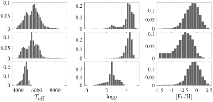
The stellar parameters distributions are shown in Figure 1. The training sample is dominated by F, G, and K stars with solar like abundance. The stars in APOGEE are mainly giants, while most of the stars in LAMOST and SSPP belong to main sequence. The RAdial Velocity Experiment (RAVE) isn’t included in the training sample, and we apply the RAVE stars to the blind test in Section 2.4.

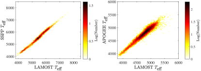
We check the overlaps between LAMOST, SSPP and APOGEE, and present the one-to-one correlations of the stellar temperatures in Figure 2. There are deviations among three catalogs, which is mainly due to the difference of the pipelines (Luo et al., 2015). Such systematic uncertainties are present in Section 2.4. We here don’t select or remove these overlap stars or the stars that observed multiple times. These stars share equal weight in our regression, and the deviations among catalogs or among observations are going to be propagated to the uncertainties of results.

2.2. Synthetic Photometry

In order to derive extinction for the training stars, we use the BT-Dusty grid (Allard 2009; Allard et al. 2011, Allard et al. 2012) of the PHOENIX photospheric model at Theoretical Model Services (TMS) to calculate a synthetic color, BP $-$ RP, and compare it to the color in $Gaia$ DR2. The synthetic color depends on three stellar parameters, $T_{\mathrm{eff}}$, log$g$ and [Fe/H], which is different from the temperature-dependent color used in Andrae et al. (2018). We adopt the transmission curves of $Gaia$ DR2 passbands . Different curves would result in different colors and introduce uncertainties to the results (Maíz Apellániz, & Weiler, 2018), but such difference is unobvious, about some mmag.

Figure 3.— One-to-one extinction correlations. Upper panel: the correlation between the $E$(BP $-$ RP) in $Gaia$ DR2 and in our training sample. Lower panels: LAMOST $A_{V}$ (left) and APOGEE $A_{Ks}$ (right) estimated by Bayesian methods vs. the $E$(BP $-$ RP) in our training sample. The best linear fits are shown as the blue dashed lines. The color bars are the density of the stars in the logarithmic scale.

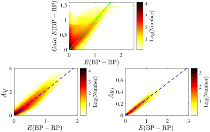
We present the one-to-one correlations between the $E$(BP $-$ RP) in $Gaia$ DR2 and those derived from the spectrum-based results in Figure 3. In the upper panel, the outliers remain at $E$(BP $-$ RP) $\sim$ 0 with $Gaia$ $E$(BP $-$ RP) $>$ 1.5 is due to the outlier filtration (Andrae et al., 2018; Arenou et al., 2018). Except these outliers, there are still many stars with the extinction overestimated by $Gaia$ DR2. It is expected, since the $T_{\mathrm{eff}}$ is underestimated by $Gaia$ (Figure 3 in Bai et al. 2019b). A lower temperature would result in higher extinction for the same sample.

A novel Bayesian method developed by Pont, & Eyer (2004) and Binney et al. (2014) has been used for stars in the LAMOST survey (Wang et al., 2016a), which has demonstrated the ability to obtain accurate distance and extinction. There are 1,062,590 cross-matched stars with valid extinction in their catalog. The one-to-one correlation is shown in the lower-left panel of Figure 3. The best linear fit is $A_{V}$ = (2.138$\pm$0.001) $\times$ $E$(BP $-$ RP). Wang et al. (2016b) has applied a similar method on APOGEE stars to estimate their distance and extinction. We cross match these stars with our training sample, and there are 65,471 stars left. The best fit is $A_{Ks}$ = (0.2752$\pm$0.0003) $\times$ $E$(BP $-$ RP). These two good linear relations indicate that our extinction is consistent with other spectrum-based results.

2.3. Algorithm

The bagged regression tree of RF algorithm (Breiman, 2001) is adopted to build the regressor. In brief, the working theory of the RF is that it builds an ensemble of unpruned decision trees and merges them together to obtain a more accurate and stable prediction. One big advantage of RF is fast learning from a very large number of data. This algorithm has been widely used for classification, while the RF regression isn’t popular. An important example of RF regression is Miller et al. (2015), and one of the best introduction of RF is Hastie et al. (2009).

We add two additional parameters, temperatures and their uncertainties given by Bai et al. (2019b), to the combination of the input: $T_{\mathrm{eff}}$, $\Delta$$T_{\mathrm{eff}}$, $l$, $b$, $\varpi$, $\Delta\varpi$, $\mu_{\alpha}$, $\mu_{\delta}$, BP $-$ $G$ and $G$ $-$ RP. Such combinations has the best performance on the $T_{\mathrm{eff}}$ regression, and it would be the best way to decouple the extinction from the temperatures.

Then, we apply the 20 folded cross validations to test the performance of the regression. The cross validation partitions the sample into twenty randomly chosen folds of roughly equal size. One fold is used to validate the regression that is trained using the remaining folds. This process is repeated twenty times such that each fold is used exactly once for validation. The 20 folded cross validation can provide an overall assessment of the regression.

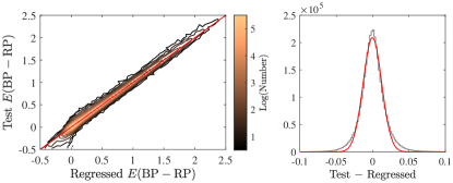
The one-to-one correlation of the cross validations is shown in the left panel in Figure 4. The Gaussian fit to the total residuals is shown in the right panel, and the fitted offset ($\mu$) and the standard deviation ($\sigma$) are listed in Table 1.

The importance estimates of the regression are shown in Figure 5. The temperature becomes the most important parameter, while other parameters have similar importance. This proves that it is effective to add $T_{\mathrm{eff}}$ to the combination of the input parameters. The importance of proper motions is lower than those of the $Gaia$ colors, which is different to the results in Bai et al. (2019b). This implies that its less relevant than colors in our extinction regressing process.

Figure 4.— The results of the cross validations. Left panel: one-to-one correlation of the cross validation . The color bar is the density contour in the logarithmic scale. Gaussian fit (red) of the total residual (black) is shown in the right panel.

Figure 5.— Important estimates of the regressor: stellar effective temperature, parallax and its error, proper motions, Galactic position, and two $Gaia$ colors.

2.4. Blind Tests

An independent blind test is effective technology to avoid systematic flaws, such as poor construction of training/test splits, inappropriate model complexity, and misleading test metrics (Bai et al., 2019a; Guyon et al., 2019). It evaluates the prediction accuracy with data that are not in the training sample, and provides validation that a regressor is working sufficiently to output reliable results.

The RAVE is designed to provide stellar parameters to complement missions that focus on obtaining radial velocities to study the motions of stars in the Milky Way s thin and thick disk and stellar halo (Steinmetz et al., 2006). Its pipeline processes the RAVE spectra and derives estimates of $T_{\mathrm{eff}}$, log $g$, and [Fe/H] (Kunder et al., 2017). Using these parameters, Binney et al. (2014) applied a Bayesian method to estimate the interstellar extinction with the uncertainties $A_{\textrm{V}}$ $\sim$ 0.1 mag. We cross match the catalog with $Gaia$ DR2, which yields 192,483 stars.

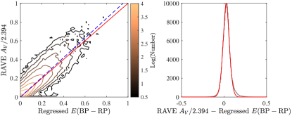
We here adopt the extinction coefficient value, 2.394 in Wang, & Chen (2019), to convert RAVE $A_{\textrm{V}}$ to $E$(BP $-$ RP), and the one-to-one correlation is shown in Figure 6. The fitted slope is close to one, 1.044 $\pm$ 0.002, and Table 1 lists the parameters of the Gaussian fit to the total residuals. These imply that our regressor is reliable, and it can determine $E$(BP $-$ RP) with fair accuracy. It should been noted that the extinction conversion in broad-band filters depends not only on the extinction law, but also on $T_{\mathrm{eff}}$, and extinction itself (Girardi et al., 2008). However, this topic is beyond the main result of this paper, and we just adopt the latest coefficient value to make a bind test.

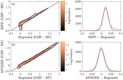
Bai et al. (2019b) applied the subregressors to test the accuracy of the regressor, since all the spectrum-based catalogs were used for training. The subregressors could also test the systematic uncertainty among different surveys. We here train the subregressors with two catalogs and use the third one to test these subregressors. The LAMOST DR5 is always included in the training set, since it accounts for 93% of the stars in our training set. We present the results of the tests in Figure 7, and list the parameters of the Gaussian fit to the total residuals in Table 1. It shows that the offsets are below 0.022 mag and standard deviations are less than 0.017 mag, which is consistent with the results of other spectrum-based methods (Wang et al. 2016a, Wang et al. 2016b).

Figure 6.— The blind test results. One-to-one correlation between the RAVE extinction and the regressed extinction is shown in the left panel. The coefficient of 2.394 (Wang, & Chen, 2019) is adopted to convert $A_{V}$ to $E$(BP $-$ RP). The best linear fit is shown as a blue dashed line. Gaussian fit (red) of the total residual (black) is shown in the right panel.

Figure 7.— Density contours of one-to-one correlations (left column) and Gaussian fits of the total residual (right column). Two catalogs are used for training and the third one for a blind test. The test catalogs are: (a) SSPP, (b) APOGEE.

Table 1Results of cross validations and blind tests

	$\mu$	$\sigma$	RMSE
Cross Validation	$-$0.3 $\pm$ 0.2	12.7 $\pm$ 0.2	18
SSPP	21.3 $\pm$ 0.4	14.3 $\pm$ 0.4	47
APOGEE	$-$1.5 $\pm$ 0.3	16.7 $\pm$ 0.3	31
RAVE	25.1 $\pm$ 0.4	37.2 $\pm$ 0.4	58

Note. — The unit is 10^-3 mag.

3. Result

Table 2Results of our regression for $Gaia$ DR2

Source ID	Regressed $E$(BP $-$ RP)
2448780173659609728	2.05 $\pm$ 0.28
2448781208748235648	0.034 $\pm$ 0.014
2448689605685695488	0.015 $\pm$ 0.019
2448689777484387072	0.490 $\pm$ 0.118
2448783991887042176	0.095 $\pm$ 0.037
2448690258520723712	0.029 $\pm$ 0.020
2448690327240200576	0.017 $\pm$ 0.018
2448689811844125184	0.529 $\pm$ 0.118
2448784953959717376	0.0454 $\pm$ 0.0126
2448783991887042048	1.25 $\pm$ 0.14

Note. — This table is available in its entirety in machine-readable form.

We now use the criteria in Bai et al. (2019b) to select qualified stars in $Gaia$ DR2, and there are 132,739,322 stars left. The feature space constructed with ten input parameters is applied to regress their $E$(BP $-$ RP), and the result is listed in Table 2.

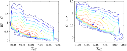
Bai et al. (2019b) suggested that external interpolation could regress results with large deviation. We plot two $Gaia$ colors as functions of the temperature in Figure 8. We use the outmost contour (log Density = 1) to separate 133 million stars into two classes, the stars located outside the contour and inside the contour. The stars located outside the contour are externally regressed in these color-temperature spaces.

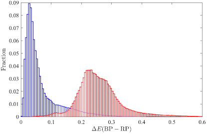
We then present the distribution of the extinction uncertainties in Figure 9, which shows that the stars located outside the contour tend to have higher deviation, larger than 0.1 mag. This indicates that we could use the uncertainty of the extinction to discriminate the result from the potential external regression. There are 106,042,018 stars with the uncertainties less than 0.1 mag.

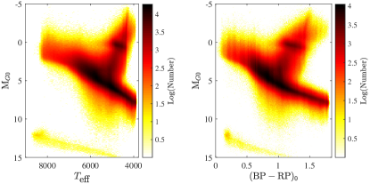
The HR-like diagrams are presented in Figure 10. Since the training sample are dominated by the A, F, G, K stars (Bai et al., 2019b), there is no stars blues than ($\textrm{BP}-\textrm{RP})_{0}$ = 0 or redder than 1.9. We could not find obvious horizontal concentrated lines in the diagram, which is different to the result of Andrae et al. (2018). The concentrated lines are probably due to the failure of temperature-extinction decoupling and the invalidation of the extinction. On the other hand, our results are tested within the parameter space covered by the spectroscopic surveys, and externally regressing them to M or B stars would suffer deviated estimates.

Figure 8.— $Gaia$ colors vs. the $T_{\mathrm{eff}}$. The contours are the densities of the stars in our training sample. The numbers are the densities in the logarithmic scale.

Figure 9.— The distribution of the extinction uncertainties. The blue histogram is the stars located inside the outmost contour in Figure 8, and the red histogram is the stars located outside the contour.

Figure 10.— HR-like diagrams for the stars with extinction uncertainties less than 0.1 mag. M_G0 vs. $T_{\mathrm{eff}}$ is in the left panel and M_G0 vs. (BP $-$ RP)₀ is in the right panel.

4. Discussion

In this work, we have attempted to regress $E$(BP $-$ RP) for 132,739,322 stars in $Gaia$ DR2 using machine learning algorithm. The regressor is trained with over three million stars in LAMOST, SSPP and APOGEE catalogs. We adopt stellar temperature, the parameters of Galactic position and two colors to build the regressor. The performance of the regression is examined with cross validations and a blind test of stars in the RAVE survey, which indicate that our regressor could predict the stellar extinction with fair accuracy. In this section we would like to discuss the comparisons with the results in other studies.

4.1. Photometry-Based Method

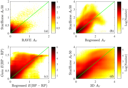
Anders et al. (2019) derived the extinction for 265 million stars using the code StarHorse, based on the combination of $Gaia$ DR2 and the photometric catalogues of Pan-STARRS1, 2MASS and AllWISE. We cross match this catalog with our result and the RAVE catalog, and present the one-to-one correlations in the upper panels of Figure 11. The $A_{V}$50 stands for the flag-cleaned 50th percentile of the line-of-sight extinction. Here we adopt the coefficient in Wang, & Chen (2019) to convert $E$(BP $-$ RP) to $A_{V}$. The consistencies are not good between the StarHorse result and those from the spectrum-based methods. The standard deviation is 0.23 mag for the panel (a) and 0.44 mag for the panel (b), about 10 times higher than our results of the cross validation and the blind tests.

We present the comparison between our results and the extinction in $Gaia$ DR2 in the panel (c) of Figure 11. The standard deviation is about 0.20 mag. There are many stars with extinction over-estimated by $Gaia$ DR2, which is similar to the distribution of the training sample. There are also some stars located at lower-right area, which aren’t shown in Figure 2. These stars are probably potential samples with the external regression, which could not be removed by the color-temperature criteria.

Another popular extinction estimate is a 3D dust map. Green et al. (2019) have presented a three-dimensional map of dust reddening, based on $Gaia$ parallaxes and stellar photometry from Pan-STARRS 1 and 2MASS. We retrieve the extinction of $Gaia$ stars with their code dustmaps, and match the result to the StarHorse catalog. The one-to-one correlation is presented in the panel (d) of Figure 11, which shows large bias with the standard deviation of 0.40 mag.

As discussed in Bai et al. (2019a), it is not an effective way to describe stellar physical environment only based on stellar photometry, since the observation conditions and the deviation estimations of different surveys are not consistent. These differences could produce additional noise, and further propagate to the results. These differences also exist in the spectrum-based surveys, but a spectrum has about a thousand data points, and it could bring much more information than multi-band photometry. These differences would become marginal, if we select spectra with high quality and similar resolution. When the signal-to-noise ratio of the input data goes up, the uncertainty goes down and a more reliable result could be acquired.

Moreover, the performance of the results is algorithm independent. The Bayesian method has been applied in the RAVE catalog, in the Wang et al. (2016a) and Wang et al. (2016b), in the Anders et al. (2019) and Green et al. (2019). The spectrum-based results share good consistency, while photometry-based results have large deviation. The volume and accuracy of the input information have a decisive influence on the overall performance of the result.

Figure 11.— One-to-one correlations. (a) $A_{V}$50 vs. RAVE $A_{V}$, (b) $A_{V}$50 vs. our result, (c) $Gaia$ extinction vs. our result, (d) $A_{V}$50 vs. 3D extinction in Green et al. (2019).

4.2. Extinction Coefficient

Wang, & Chen (2019) has presented precise multi-band coefficients for a group of 61,111 red clump stars in the APOGEE survey. Their coefficient ratio $A_{Ks}$/$A_{V}$ = 0.078 is lower than the result in our training sample $\frac{0.2752E\textrm{(BP - RP)}}{2.138E\textrm{(BP - RP)}}$ = 0.129 (Figure 3). Dutra et al. (2002) has built $K$ band extinction maps in the area of two candidate low-extinction windows in the inner Bulge, and the ratio is 0.118.

It has long been debated whether the infrared extinction law is universal (Wang et al., 2013; Wang, & Jiang, 2014). The dust may be larger in denser regions of the Galaxy, which would lead to a smaller power law index (Li et al., 2015). The APOGEE survey is in the near infrared band that could observe the stars located in the denser regions than the LAMOST survey which is in the optical wavelength. These different ratios may imply that the red clump stars of Wang, & Chen (2019) and the APOGEE stars in our training sample are located at a different regions of the Galaxy. Such difference would slightly differentiate the coefficient in the near infrared. We check the regions covered by LAMOST, SSPP and APOGEE for the stars in our training sample, and find that most of them are located at similar regions. Therefore, this difference is not obvious for the three surveys of our training sample.

References

- Allard (2009) Allard, F. 2009, A&A, 500, 93
- Allard et al. (2011) Allard, F., Homeier, D., & Freytag, B. 2011, 16th Cambridge Workshop on Cool Stars, Stellar Systems, and the Sun, 448, 91
- Allard et al. (2012) Allard, F., Homeier, D., & Freytag, B. 2012, Philosophical Transactions of the Royal Society of London Series A, 370, 2765
- Allende Prieto et al. (2008) Allende Prieto, C., Sivarani, T., Beers, T. C., et al. 2008, AJ, 136, 2070
- Andrae et al. (2018) Andrae, R., Fouesneau, M., Creevey, O., et al. 2018, A&A, 616, A8
- Anders et al. (2019) Anders, F., Khalatyan, A., Chiappini, C., et al. 2019, A&A, 628, A94
- Arenou et al. (2018) Arenou, F., Luri, X., Babusiaux, C., et al. 2018, A&A, 616, A17
- Bai et al. (2019a) Bai, Y., Liu, J.-F., Wang, S., & Yang, F. 2019a, AJ, 157, 9
- Bai et al. (2019b) Bai, Y., Liu, J., Bai, Z., Wang, S., & Fan, D. 2019b, AJ, 158, 93
- Binney et al. (2014) Binney, J., Burnett, B., Kordopatis, G., et al. 2014, MNRAS, 437, 351
- Breiman (2001) Breiman, L. 2001, in Random Forests, 45, pp 5-32
- Du et al. (2012) Du, B., Luo, A., Zhang, J., Wu, Y., & Wang, F. 2012, Proc. SPIE, 8451, 845137
- Dutra et al. (2002) Dutra, C. M., Santiago, B. X., & Bica, E. 2002, A&A, 381, 219
- Hastie et al. (2009) Hastie, T., Tibshirani, R., & Friedman, J., The Elements of Statistical Learning, Springer Series in Statistics, 2009, Section 15, 587
- Gaia Collaboration et al. (2016) Gaia Collaboration, Prusti, T., de Bruijne, J. H. J., et al. 2016, A&A, 595, A1
- Gaia Collaboration et al. (2018) Gaia Collaboration, Brown, A. G. A., Vallenari, A., et al. 2018, A&A, 616, A1
- Gao et al. (2015) Gao, H., Zhang, H.-W., Xiang, M.-S., et al. 2015, Research in Astronomy and Astrophysics, 15, 220
- García Pérez et al. (2016) García Pérez, A. E., Allende Prieto, C., Holtzman, J. A., et al. 2016, AJ, 151, 144
- Girardi et al. (2008) Girardi, L., Dalcanton, J., Williams, B., et al. 2008, PASP, 120, 583
- Green et al. (2019) Green, G. M., Schlafly, E. F., Zucker, C., Speagle, J. S., & Finkbeiner, D. P. 2019, arXiv:1905.02734
- Guyon et al. (2019) Guyon I. et al. Analysis of the AutoML Challenge Series 2015 C2018. In: Hutter F., Kotthoff L., Vanschoren J. (eds) Automated Machine Learning. The Springer Series on Challenges in Machine Learning. Springer, Cham 2019, pp 177-219
- Koleva et al. (2009) Koleva, M., Prugniel, P., Bouchard, A., & Wu, Y. 2009, A&A, 501, 1269
- Kunder et al. (2017) Kunder, A., Kordopatis, G., Steinmetz, M., et al. 2017, AJ, 153, 75
- Lee et al. (2008a) Lee, Y. S., Beers, T. C., Sivarani, T., et al. 2008a, AJ, 136, 2022
- Lee et al. (2008b) Lee, Y. S., Beers, T. C., Sivarani, T., et al. 2008b, AJ, 136, 2050
- Li et al. (2015) Li, A., Wang, S., Gao, J., & Jiang, B. W. 2015, Lessons from the Local Group: A Conference in honor of David Block and Bruce Elmegreen, 85
- Luo et al. (2015) Luo, A.-L., Zhao, Y.-H., Zhao, G., et al. 2015, Research in Astronomy and Astrophysics, 15, 1095
- Maíz Apellániz, & Weiler (2018) Maíz Apellániz, J., & Weiler, M. 2018, A&A, 619, A180
- Majewski et al. (2017) Majewski, S. R., Schiavon, R. P., Frinchaboy, P. M., et al. 2017, AJ, 154, 94
- Mathur et al. (2017) Mathur, S., Huber, D., Batalha, N. M., et al. 2017, ApJS, 229, 30
- Mészáros et al. (2013) Mészáros, S., Holtzman, J., García Pérez, A. E., et al. 2013, AJ, 146, 133
- Miller et al. (2015) Miller, A. A., Bloom, J. S., Richards, J. W., et al. 2015, ApJ, 798, 122
- Pelisoli et al. (2019) Pelisoli, I., Bell, K. J., Kepler, S. O., & Koester, D. 2019, MNRAS, 482, 3831
- Pont, & Eyer (2004) Pont, F., & Eyer, L. 2004, MNRAS, 351, 487
- Sahlholdt et al. (2019) Sahlholdt, C. L., Feltzing, S., Lindegren, L., & Church, R. P. 2019, MNRAS, 482, 895
- Smolinski et al. (2011) Smolinski, J. P., Lee, Y. S., Beers, T. C., et al. 2011, AJ, 141, 89
- Steinmetz et al. (2006) Steinmetz, M., Zwitter, T., Siebert, A., et al. 2006, AJ, 132, 1645
- Wang et al. (2016a) Wang, J., Shi, J., Zhao, Y., et al. 2016a, MNRAS, 456, 672
- Wang et al. (2016b) Wang, J., Shi, J., Pan, K., et al. 2016b, MNRAS, 460, 3179
- Wang et al. (2009a) Wang, S., Tang, K., & Yao, X. 2009, Proc. Int. Joint Conf. Neural Netw. pp. 3259-3266
- Wang et al. (2009b) Wang, S. & Yao, X. 2009, Proc. IEEE Symp. Computat. Intell. Data Mining pp. 324-331
- Wang et al. (2013) Wang, S., Gao, J., Jiang, B. W., et al. 2013, ApJ, 773, 30
- Wang, & Jiang (2014) Wang, S., & Jiang, B. W. 2014, ApJ, 788, L12
- Wang, & Chen (2019) Wang, S., & Chen, X. 2019, ApJ, 877, 116
- Wu et al. (2014) Wu, Y., Du, B., Luo, A.L., et al. 2014, IAUS, 306, 340
- Yanny et al. (2009) Yanny, B., Rockosi, C., Newberg, H. J., et al. 2009, AJ, 137, 4377