Deep Reinforcement Learning for Motion Planning of Mobile Robots

Abstract

This paper presents a novel motion and trajectory planning algorithm for nonholonomic mobile robots that uses recent advances in deep reinforcement learning. Starting from a random initial state, i.e., position, velocity and orientation, the robot reaches an arbitrary target state while taking both kinematic and dynamic constraints into account. Our deep reinforcement learning agent not only processes a continuous state space it also executes continuous actions, i.e., the acceleration of wheels and the adaptation of the steering angle.

We evaluate our motion and trajectory planning on a mobile robot with a differential drive in a simulation environment.

I Introduction

Motion planning is a well-known fundamental challenge in mobile robotics [3]. Depending on the dynamic nature of the environment and the physical constraints that are considered it soon becomes complex. Moreover, in many real world applications mobile robots are faced with highly dynamic environments and frequent changes in immediate surroundings that require quick reaction times.

Consider the soccer application depicted in Fig. 1. At least one player (blue) tries to score a goal while at least one mobile robot (orange) defends. A real-time locating system (RTLS) tracks the ball and the player kinematics and the mobile robots and delivers a stream of their positions [5, 18]. A high-level tactical analysis monitors all trajectories and generates a stream of target positions $t_{0},t_{1}...$ per robot so that the goal is best shielded at any time $t$. As inertia limits the robots’ movement flexibility we need to keep them constantly be moving. Therefore, a tactical analysis monitors the players’ movement patterns and also generates appropriate orientations and velocities for the prospective target positions. These together describe a target state that is then used to estimate a trajectory for the robot (even before it reaches its current target state, see $t_{2}$).

Sampling methods [13] estimate such trajectories by reducing the continuous control problem to a discrete search problem. But the reduction in complexity comes with a loss in optimality and completeness of the solution which in turn can lead to unsatisfying results in such highly dynamic environments [13]. However, while it is possible to find such a trajectory through analytical methods [16] it becomes significantly more challenging if we also consider the kinematic and dynamic side constraints. This leads to a non-linear optimization problem that can no longer be solved analytically fast enough for such interactive scenarios.

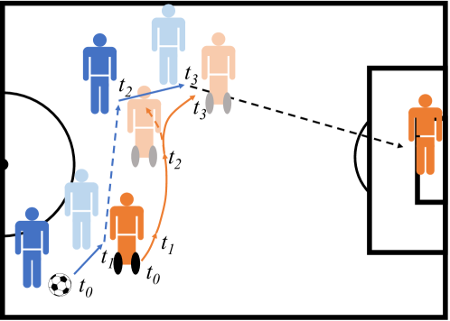
Figure 1: Mobile robots interact with humans in a dynamic soccer application.

To address the full motion estimation problem we use recent advances in deep reinforcement learning and teach a robot to generate feasible trajectories that obey kinematic and dynamic constraints in real-time. A simulation environment models the environmental and physical constraints of a real robotic platform. We generate random target states and let a deep reinforcement learning (RL) agent based on Deep Deterministic Policy Gradient (DDPG) [15] interact with the simulator on a trial-and-error basis to solve the motion planning problem within a continuous state and action space.

The remainder of this paper is structured as follows. Sect. II discusses related work and Sect. III provides background information. Next, we show our main contributions: we formalize the problem and describe the implementation of our reward-system and RL agent in Sect. IV. Sect. V evaluates our approach with a deep RL-agent within a simulation environment that also models the robot’s and environmental physics before Sect. VI concludes.

II Related Work

Trajectory planning [6] generates a sequence of control inputs based on a geometric path and a set of kinematic or dynamic constraints. The geometric path comes from path planning methods. Both together solve the motion planning problem. While they are typically decoupled [3] some approaches solve the motion planning problem directly [3].

Sampling-based approaches discretize the action and state space, and transform the underlying control problem into a graph search problem [14], which allows for the use of precomputed motion primitives [9, 20, 19]. Further extensions propose better-suited cost functions [12] for the search algorithms, e.g. state lattice planners [23, 26] sample the state space with a deterministic lattice pattern. Randomness [13] helps to reduce generated trajectories that are not relevant for the given search problem. While sampling-based approaches are not complete, they offer probabilistic completeness [10, 13], i.e., the probability to find a solution grows with the runtime. However, as sampling based approaches discretize the state and action space, they require a high amount of computational resources [16] to account for all possible motions. In general, a higher number of motion primitives leads to a rapid growth in time complexity [17]. Realistic motion planners need thousands of such primitives and are therefore not suitable for a interaction [17].

Interpolation-based methods use way points to compute a path with higher trajectory continuity. In the simplest case they interpolate with lines and circles. More elaborate approaches use clothoid curves [1], polynomial curves [7] and Bézier curves [21]. Clothoid curves allow for the definition of trajectories based on linear changes in curvature since their curvature is defined as their arc-length [1]. Polynomial curves are commonly used to also take side-constraints into account, since their coefficients are defined by the constraints in their beginning and ending segments [7]. Bézier curves are defined by a set of control points and represent parametric curves [21]. However, the trajectories are not necessarily optimal and although these methods may generate smooth trajectories they may also not obey kinodynamic side-constraints.

Numerical optimization extends both sampling- and interpolation-based algorithms. Kinematic and dynamic constraints require additional optimization. Numerical optimization generates trajectories based on a differentiable cost function and side-constraints. Under convex cost and constraint functions [16] they find globally optimal trajectories [24]. Either they optimize a suboptimal trajectory [4] or compute a trajectory on predefined constraints [25]. Such planners generate continuous trajectories by optimizing a function that considers planning parameters like position, velocity, acceleration and jerk [25, 24]. However, the downside of the additional optimization step is the rise in time complexity. While a suboptimal trajectory can be computed quickly, an optimal solution is time consuming [11] and therefore less applicable for time-critical tasks.

Since we need a fast and frequent (re-)computation of (ideally near-optimal) trajectories that obey kinodynamic side-constraints existing methods are not sufficient. Instead, our deep reinforcement learning is trained offline and delivers trajectories satisfying all side-constraints in real-time given a continuous action and state space.

III Background on Reinforcement Learning

The key idea behind reinforcement learning is an agent that interacts with the environment, see Fig. 2. In each time step the agent receives an observation $s_{t}$, i.e., some (partial) information on the current state, and selects an action $a_{t}$ based on the observation. The environment then rewards or punishes this action with a reward $r_{t+1}$.

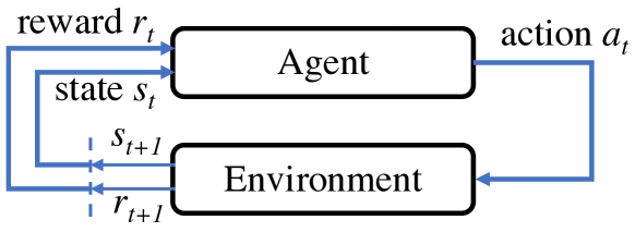
Figure 2: The basic reinforcement learning scenario.

III-A Markov Decision Process

A reinforcement learning task that satisfies the Markov property, i.e, that the probabilities of future states $s_{T>t}$ only depend on the state $s_{t}$ but not on previous events, is called a Markov Decision Process (MDP). With a set of states $s\in S$, actions $a\in A$, and rewards $r\in R$ a controlled process with Markov dynamics at time $t=0,1,...$ is defined by

$$p(s^{\prime}|s,a) =\text{Pr}(s_{t+1}=s^{\prime}|s_{t}=s,a_{t}=a)\text{, and}$$

$$r(s,a,s^{\prime}) =\mathbb{E}[R_{t+1}|s_{t}=s,a_{t}=a,s_{t+1}=s^{\prime}],$$

where $p(s^{\prime})$ is defined by a probability distribution that models the transition dynamics (as often state transition may be probabilistic) and $r(s,a,s^{\prime})$ is defined by the expected reward if we choose action $a_{t}$ in $s_{t}$ and end up in $s_{t+1}$.

In fully observed environments an observation $o_{t}$ completely describes the underlying (real) state of the environment $s_{t}$. However, in partially observable environments the agent must estimate the real state $s_{t}$ based on $o_{t}$ or a set of past and present observations. For simplification we consider a fully observable environment, i.e., we assume $o_{t}=s_{t}$.

III-B Reinforcement Learning

We use the state-value function $v^{\pi}(s)$ to denote the value of state $s$ under a given policy $\pi$, i.e., the expected total reward given that the agent starts from state $s$ and behaves according to $\pi$. Accordingly, the value of a state is defined as the (expected) sum of discounted future rewards

$\displaystyle v_{\pi}(s)=\mathbb{E}_{\pi}\left[G_{t}|S_{t}=s\right]=\mathbb{E}_{\pi}\left[\sum_{k=0}^{\infty}\gamma^{k}R_{t+k+1}|S_{t}=s\right],$

where $\mathbb{E}\left[\cdot\right]$ denotes the expected value, $t$ is any time step, and $\gamma\in\left[0,1\right]$ is the discount factor that favors immediate rewards over future rewards (and that also determines how far in the future the rewards are considered). The goal of reinforcement learning lies in the maximization of the expected discounted future reward from the initial state.

The policy $\pi:$ $S\rightarrow P(A)$ maps a state $s\in S$ to a probability distribution over the available actions $a\in A$. Since the future actions of the agent are defined by the policy $\pi$ and the state transitions by the transition dynamics $p(s_{t+1}|s_{t},a_{t})$ we can estimate the future reward that we can expect in any given state.

Similarly, we can define the value of taking action $a$ in state $s$ under a policy $\pi$ as the expected return starting from $s$, taking the action $a$, and thereafter following policy $\pi$:

$$q_{\pi}(s,a) =\mathbb{E}_{\pi}\left[G_{t}|S_{t}=s,A_{t}=a\right]$$

$$=\mathbb{E}_{\pi}\left[\sum^{\infty}_{k=0}\gamma^{k}R_{t+k+1}|S_{t}=s,A_{T}=a\right],$$

which is called the (state-)action-value function for policy $\pi$. The recursive formula describes the relationship between the value of a state and the value of the successor states and is also often called Bellman equation for $v_{\pi}$.

To learn the optimal action-value function is one of the central goals of reinforcement learning. Popular methods are dynamic programming, on- and off-policy monte-carlo-methods, temporal-difference learning, and Q-learning.

III-C Deep Deterministic Policy Gradient (DDPG)

Value-based reinforcement learning such as Q-learning has poor convergence properties as slow changes in the value estimate have a big influence on the policy. Instead, policy-based reinforcement learning directly updates the policy but often converges to local optima.

Actor-critic-methods combine the best of both worlds, see Fig. 3. Instead of directly estimating the state-action-value function we use two separate components. While a critic estimates the value of state-action-pairs an actor takes a state $s_{t}$ and estimates the best action from within this state.

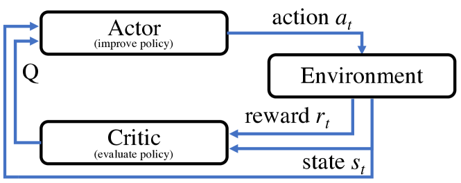
Figure 3: Actor-critic framework.

The combination of an actor-critic-framework and deep neural networks allows the application of Q-learning to a continuous state and action space [15]. DDPG uses a parameterized actor-function $\mu(s|\theta^{\mu})$ and critic-function $Q(s,a|\theta^{Q})$, where $\theta^{\mu}$ and $\theta^{Q}$ are the weight parameters of neural networks that approximate these functions.

The critic function is learned using the the Bellman equation and standard back-propagation. As learning through neural networks in RL is unstable DDPG uses a concept of target networks, i.e., $Q^{\prime}$ and $\mu^{\prime}$, to ensure that the critic’s network updates only change slowly. The target networks are initialized by copying the actor and critic networks and then updated using $\tau\ll 1$ through

$$\theta^{\prime} \leftarrow\tau\theta+(1-\tau)\theta^{\prime}\text{, and}$$

$$\mu^{\prime} \leftarrow\tau\mu+(1-\tau)\mu^{\prime}.$$

To train the actor we use the chain rule to the expected return from the start distribution with respect to the actor parameters. To better explore the action space we sample from a normal distribution and add it to the actor policy.

To allow for minibatch (learning from a batch of transitions) and off-policy learning, as well as the i.i.d assumption (independent and identically distributed), DDPG uses a replay buffer that stores transitions $(s_{t},a_{t},r_{t},s_{t+1})$ after each interaction from which we later sample for training.

IV Method

IV-A Kinematic Model

Although our application assumes a differential drive mobile robot we model the robot by a unicycle with a clearer physical interpretation as both kinematics are equivalent [22]. Hence, its configuration is given by $q=[x\ y\ \theta]^{T}$, with wheel orientation $\theta$ and the contact point of the wheel with the ground $(x,y)$. The kinematic model is described by

$$\begin{bmatrix}\dot{x}\\ \dot{y}\\ \dot{\theta}\end{bmatrix} =\begin{bmatrix}cos\theta\\ sin\theta\\ 0\end{bmatrix}\nu+\begin{bmatrix}0\\ 0\\ 1\end{bmatrix}\omega,$$

where $\nu$ is the velocity and $\omega$ is the steering velocity.

IV-B Dynamic Constraints

We also consider physical limitations known from real physical robot platforms. We limit the linear acceleration $\Delta\nu$ and the angular acceleration $\Delta\omega_{target}$ by

$$|\Delta\nu| \leq a_{max,linear}\cdot dt\text{, and}$$

$$|\Delta\omega_{target}| \leq a_{max,angluar}\cdot dt$$

in each time step $dt$. As we need to prevent the robot from tipping over we also include centrifugal force limits:

$$|\nu_{target}\cdot\omega_{target}|\leq a_{max,lateral}.$$

We also restricted the steering to a maximum velocity $|\nu|\leq\nu_{max}$ and an angular rate $|\omega|\leq\omega_{max}$.

IV-C Problem Formulation

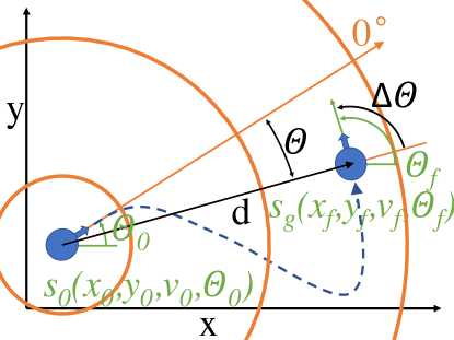
Figure 4: Formulization of the motion planning problem.

In accordance to our kinematic model we describe a state $s$ by $(x,y,\nu,\theta)^{T}$, where $x$ and $y$ are the robot’s Cartesian coordinates, $\nu$ its linear velocity, and $\theta$ its forward orientation.

To formalize our motion planning consider Fig. 4. The robot’s task is to reach a goal state $s_{g}$ from a start state $s_{0}$. We consider a control affine non-linear dynamic system with drift dynamics and stochastic effectiveness of control inputs. Both are unknown, but are assumed to be locally Lipschitz functions, i.e., locally constant. We also assume the control effectiveness function to be bounded.

Our RL-Agent receives a new observation $o_{t}$ and a reward $r_{t}$ per time-step $t$ for the current and past actions from our environment. We define an observation by $o_{t}=\big{(}d,\theta,\Delta\nu,\Delta\theta,\nu,\phi\big{)}$, where $(d,\theta)$ is the polar coordinate of the goal position in the robot’s frame, $\Delta\nu$ is the residual of the current to the goal velocity, $\Delta\theta$ is the residual of the (global) current to the goal orientation, and $(\nu,\phi)$ are the actual velocity and rotation rate of the robot. The latter two ensure a fully observable environment to our agent.

We relax the motion planning constraints and allow the robot to reach the goal-state both forwards and backwards as long as its motion vector is correct. Therefore, the residual of the velocity $\Delta\nu$ is $\nu_{f}-|\nu|$ and

$$\Delta\theta=\theta_{f}-\left\{\begin{tabular}[]{@{}l@{\quad}l@{}}$\theta$&if $\nu\geq 0$\\ $\theta+\pi$&if $\nu<0$.\end{tabular}\right.$$

Afterwards we normalize $\Delta\theta$ to $]$$-\pi,\pi$$]$.

Our simulation environment returns an immediate reward $r_{t}=\frac{1}{1+e}$, where the error $e=\left|\left|\hat{s}_{g}-\hat{s}_{t}\right|\right|_{2}$ is the Euclidean distance between the current state $\hat{s_{t}}$ and the goal state $\hat{s}_{g}$.

We end an episode, if either the error is lower than a threshold $e<\varepsilon$ or if we reach a maximum number of steps $t\geq T$. In the former case, the agent receives an additional fixed reward $R$ at the last step to enforce this behavior as the reward alone does not tell the agent how time-efficient its trajectory has been.

Fig. 5 shows how a discounted reward (orange line) helps to score for time-optimality. The closer a state is to our final goal state $s_{g}$ the higher is the discounted reward for the agent (e.g. it is higher at $s_{n}^{\prime}$ than at $s_{n}$). This encourages the agent to move closer to $s_{g}$ at a later point. The orange curve is mainly influenced by the final reward $r_{g}=R$ if the agent has reached the goal state $s_{g}$. If the agent does not reach the goal state the orange curve uses the discounted immediate reward $r_{t}$, which is much smaller. However, this smaller reward initially helps the agent to find the goal state in the search space.

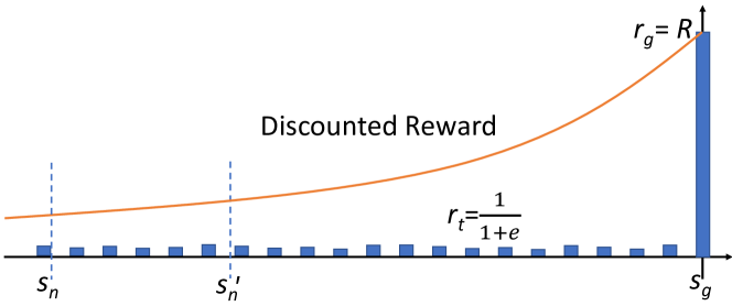
Figure 5: Discounted Reward.

V Evaluation

We use a simulator (Sect. V-A) to train our RL-agent (Sect. V-B). We evaluate the optimization of our agent during training (Sect. V-C) before we show the efficiency of our RL-based approach (Sect. V-D). We also evaluate our approach in a complex use-case scenario (Sect. V-E).

V-A Simulation and Training Setup

To train and test our RL-based motion planner we implemented the environment, i.e., the kinodynamic constraints, the kinematic model, our reward system, and the action, observation and state scheme, within the OpenAI Gym framework [2]. We implemented a discrete form with a step-size of $dt=0.1s$ and applied the following kinematic constraints: $a_{max,linear}$=$2.2\frac{m}{s^{2}}$, $a_{max,angular}$=$2.0\frac{m}{s^{2}}$, $a_{max,lateral}$=$1.0\frac{m}{s^{2}}$, $\nu_{max}$=$4.0\frac{m}{s}$ and $\omega_{max}$=$4.5\frac{1}{s}$.

To let our agent learn, we generate random pairs of start- and goal-states. We transform them such that the start-state is at the origin $(0,0)$ and its initial orientation points to the positive x-axis, and sample its velocity ($0...v_{max}$) from a uniform distribution. We generate the goal-state in relation to the local frame within a position sampled uniformly within a distance of $]0.5m...5.0m]$ to the origin. We also sample the goal orientation and velocity uniformly. Note, that we allow to reach the goal state backwards or forwards, i.e., the orientation then turns by $180^{o}$ with a negative velocity.

The agent gets a reward $R$=$100$ if it reaches the final goal-state within a threshold of $e<0.5$. We used a grid search to evaluate the reward $R\in\{1,10,100\}$. We end an episode if the agent needs more than $200$ steps to reach the goal. In this case, the last reward is the immediate reward $r_{t}$.

For both training and testing the agent and the simulator run on a desktop machine equipped with an Intel Core i7-7700 CPU@3.60GHz (4 cores, 8 threads), 32GB memory, and an Nvidia GeForce GTX1070 with 8GB memory. We implemented all our algorithm in Python.

V-B Training Parameters of the RL-Agents

Our DDPG agent uses two separate networks for the actor and the critic that have a similar design. Both use an input layer, three fully connected hidden layers (with 200 neurons each) and an output layer. The hidden layers are necessary to approximate the non-linearities in the value-function. Both the actor and the critic receive the observation vector $o_{t}$ at the input layer. The actor output is additionally connected to the second hidden layer of the critic. We use a linear action (ReLU) for the critic’s output layer and tanh-activation in all other cases. While we initialize all biases with a constant value of $0.1$, we initialize the weights of the critic by sampling from a normal distribution $\mathcal{N}$($\mu$=$0$, $\sigma^{2}$=$0.1$) and the actor by sampling from $\mathcal{N}$($\mu$=$0$, $\sigma^{2}$=$0.3$).

For the training using back-propagation we use the ADAM optimizer. The exploration in our DDPG agent uses a simple $\epsilon$-greedy algorithm. We evaluated the following combinations with a grid search to find the best hyperparameters for the training (best setting in bold): learning rate actor ($\alpha\in\{10^{-1},\mathbf{10^{-2}},10^{-3},10^{-4},10^{-5}\}$, $\beta_{1}$=$0.9$, $\beta_{2}$=$0.999$, $\epsilon$=$10^{-8}$) learning rate critic ($\alpha\in\{10^{-3},\mathbf{10^{-4}},10^{-5},10^{-6},10^{-7}\}$, $\beta_{1}$=$0.9$, $\beta_{2}$=$0.999$, $\epsilon$=$10^{-8}$), discount factor $\gamma\in\{0.5,0.8,0.9,\mathbf{0.95}\}$, batch size $\in\{\mathbf{500},1000,2000\}$ (has no influence since it’s indirect proportional to the training time), exploration probability $\epsilon\in\{\mathbf{0.5},0.75\}$, exploration variation $\sigma\in\{\mathbf{3.0},5.0\}$, memory size ($50000$), and soft update factor $\tau=0.1$.

For the test we set $\epsilon$=$0$ to fully exploit the policy. While the immediate output of the actor is a greedy action we select a non-greedy action by sampling from a normal distribution with the greedy action as its mean: $a^{\prime}$=$\mathcal{N}(a,\sigma)$. The variance in training defines the randomness of the action: with a higher variance we more likely choose random actions.

V-C Optimization during Training

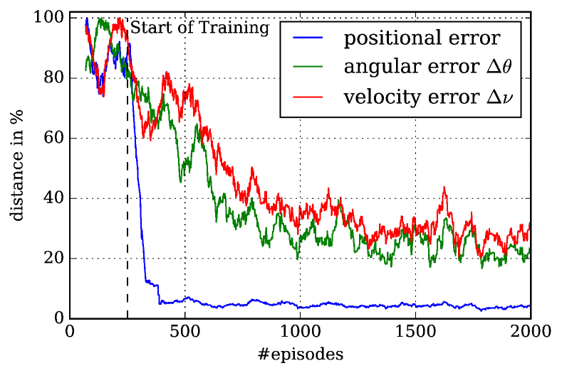
Figure 6: Distance per dimension on training for the 4-dimensional problem.

To understand how our agent optimizes the motion planning we train the agent in the 4D state space and analyze the error on the particular dimensions over the training episodes.

Fig. 6 shows the distance/error of the 4D-agent per state dimension, i.e., positional distance, angular distance $\Delta\theta$, and velocity distance $\Delta\nu$, over the training episodes. As we now only focus on the optimization of each individual dimension we scale the y-axis to show the results in percentages (the maximal positional distance was $14.0$m, the maximal angular distance was $179.7\degree$, and the maximal velocity distance was $3.88$m/s). The episodes that the agent run until the dashed line at episode #250 are (until that point) only used to fill the replay memory. They are generated using the randomly initialized policy.

Afterwards, the agent samples from the replay memory and starts training with a absolute positional error of around $14$m, and angular error of approx. $90\degree$ and a velocity error of $1.7$m/s (max. $4.0$m/s allowed). The agent optimizes for the positional error first. It drops below $1.0$m after only 500 episodes, i.e., 250 episodes in training. The optimization of the angular error comes with a little delay: it drops below $40\degree$ at episode 1,000. The agent optimizes for the velocity at latest. Starting with an error of $1.7$m/s the error drops below $0.6$m/s after 1,700 episodes. Interestingly, velocity and angular distance fight for a minimum error until the end. Note that the errors are higher during training as the agent applies a non-greedy behavior.

V-D Accuracy Results

The agent’s task is to reach a goal-state with time- and way-efficient controls. However, as the 4D problem is complex we break it down to subproblems on which we analyze our agent’s behavior.

We separately train an agent and evaluate its accuracy within the 2D- (only position), 3Da- (position and orientation), 3Db- (position and velocity), and 4D-problem (complete goal-state). Hence, we trained four agents using the same reward function for 4,000 episodes each. The total training time has been 45 minutes for all agents in parallel.

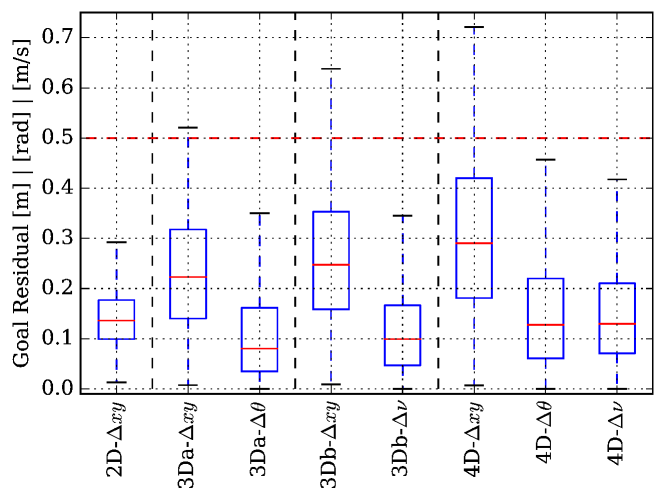
Figure 7: Accuracy per problem dimension.

We later evaluated the performance of the agents with randomly sampled start and goal state-pairs, see Sect. V-A. Fig. 7 shows the results for the four agents. For each agent we separately plot the errors in the different dimensions.

The positional error is best for the 2D-problem (mean of $0.14$m) and increases as the problem becomes more complex, i.e., a mean error of $0.23$m (3Da), $0.31$m (3Db), and $0.39$m (4D). The mean angular error of $6.3\degree$ in the 3Da-problem also increases a bit to $10.3\degree$ for the 4D-problem. The velocity error behaves similarly: from $0.14$m/s in 3Db is increases to $0.20$m/s in the 4D-case. Please note, that the plot shows the median error, which is a bit smaller.

What we do not see here is that the agents achieved success rates (i.e., that the error is below a threshold of 0.5) of $100.0\%$ (2D), $99.9\%$ (3Da), $99.0\%$ (3Db) and even $97.6\%$ (4D) for a total number of 1,000 testing episodes. With increasing dimensions the problem becomes more complex and harder to solve. However, the 4D-agent even solves the complex motion planning task in most of the cases and satisfies all kinodynamic side-constraints at any time

We also compared the time-efficiency of the generated trajectories to a cubic spline derived from a velocity ramp. The spline’s velocity starts from the initial velocity in the start state, increases to the maximum possible velocity, and decreases to the target velocity at the latest point. This achieves maximal linear acceleration and maximal velocity by design. But as the spline interpolation does not consider kinematic constraints most of the generated trajectories are not feasible. However, we use them to estimate a base-line for the duration of the generated trajectories.

The mean and standard deviation of the duration ratio between the spline base-line and our agent for the different subproblems was $(\mu=0.66;\sigma=0.04)$ (2D), $(0.81;0.08)$ (3Da), $(0.81;0.26)$ (3Db), and $(1.29;0.55)$ (4D). Our RL-approach generates faster trajectories than the spline-based approach in the 2D, 3Da and 3Db case. But the 4D-agent’s trajectories take $1.29$ times longer. However, this is the tradeoff between time-efficiency and kinodynamic side-constraints as the trajectories of the RL-agent are feasible while the spline-based trajectories are not.

V-E Application Results

To evaluate our approach for the use case we initially introduced we implemented a composite task that continuously updates the goal-states, see Fig. 8. We generate four goal-states a-priori. The green vectors describe the states: the goal position is the start of the vector, the length describes the velocity (also labeled) and the vector’s orientation the goal orientation of the robot at that state. The agents did not see this scenario or such a situation within their training phase explicitly (although similar combinations might have been included in the training episodes).

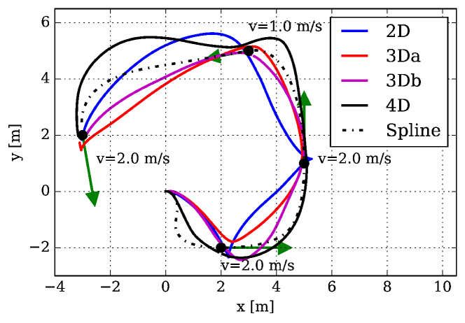
Figure 8: Application test scenario.

Fig. 8 shows the trajectories of the trained agents from Sect. V-D. The dotted line denotes the spline-based trajectory, which again, is not said to satisfy the constraints at any time. We see that the lower dimensional agent D2 steers to the desired goal positions but generates unsteady trajectories near the goal states. Considering the introductory use case, a motion planner that generates trajectories only based on positions will fail to react fast enough (as it introduces in-place rotations and zero velocities, see the first goal point). The 3Da-agent behaves much more smoothly and generates correct orientations, but fails for the last goal point where the orientation is achieved by an in-place rotation. The 3Db-agent is better and generates a smooth trajectory. However, it may still also fail if the tactical analysis updates the goal state that then might be at an unprofitable position.

But the 4D-agent not only gets close to the spline base-line but also considers all kinodynamic constraints that are violated by the spline between the third and fourth goal-point. The agent achieves a smooth and way-efficient steering to reach goal-points only by exploiting the learned behavior.

VI Conclusion

This papers presents a motion planning based on deep reinforcement learning. In contrast to previous research in motion planning our algorithm does not compute trajectory plans a-priori or on-demand but rather delivers a stream of control commands that we can use directly to steer a robot. Our approach uses a reward function, state representation and a framework which we used to train an Deep Deterministic Policy Gradient (DDPG) agent.

We evaluated our approach in a simulation environment and compared it to a spline-interpolation. We also proved the applicability of our approach in a dynamic use-case that continuously provides updated goal states.

References

- [1] M. Brezak and I. Petrović. Real-time approximation of clothoids with bounded error for path planning applications. IEEE Trans. Robotics, 30(2):507–515, 2014.
- [2] G. Brockman, V. Cheung, L. Pettersson, J. Schneider, J. Schulman, J. Tang, and W. Zaremba. Openai gym, 2016.
- [3] H. M. Choset. Principles of robot motion: theory, algorithms, and implementation. MIT press, 2005.
- [4] D. Dolgov, S. Thrun, M. Montemerlo, and J. Diebel. Path planning for autonomous vehicles in unknown semi-structured environments. Intl. J. Robotics Research, 29(5):485–501, 2010.
- [5] T. Feigl, T. Nowak, M. Philippsen, T. Edelhäußer, and C. Mutschler. Recurrent Neural Networks on Drifting Time-of-Flight Measurements. In 9th Intl. Conf. Indoor Positioning and Indoor Navigation, 2018.
- [6] A. Gasparetto, P. Boscariol, A. Lanzutti, and R. Vidoni. Trajectory planning in robotics. Mathematics in Comp. Sc., 6(3):269–279, 2012.
- [7] S. Glaser, B. Vanholme, S. Mammar, D. Gruyer, and L. Nouveliere. Maneuver-based trajectory planning for highly autonomous vehicles on real road with traffic and driver interaction. IEEE Trans. Intelligent Transportation Systems, 11(3):589–606, 2010.
- [8] N. Heess, J. J. Hunt, T. P. Lillicrap, and D. Silver. Memory-based control with recurrent neural networks. CoRR, abs/1512.04455, 2015.
- [9] T. M. Howard, C. J. Green, A. Kelly, and D. Ferguson. State space sampling of feasible motions for high-performance mobile robot navigation in complex environments. J. Field Robotics, 25(6-7):325–345, 2008.
- [10] D. Hsu, J.-C. Latombe, and H. Kurniawati. On the probabilistic foundations of probabilistic roadmap planning. Intl. J. Robotics Research, 25(7):627–643, 2006.
- [11] M. Kalakrishnan, S. Chitta, E. Theodorou, P. Pastor, and S. Schaal. Stomp: Stochastic trajectory optimization for motion planning. In IEEE Intl. Conf. Robotics and Automation, pages 4569–4574, 2011.
- [12] S. M. LaValle. Planning algorithms. Cambridge University Press, New York, NY, 2006.
- [13] S. M. LaValle and J. J. Kuffner Jr. Randomized kinodynamic planning. Intl. J. Robotics Research, 20(5):378–400, 2001.
- [14] M. Likhachev, D. Ferguson, G. Gordon, A. Stentz, and S. Thrun. Anytime search in dynamic graphs. Artificial Intelligence, 172(14):1613–1643, 2008.
- [15] T. P. Lillicrap, J. J. Hunt, A. Pritzel, N. Heess, T. Erez, Y. Tassa, D. Silver, and D. Wierstra. Continuous control with deep reinforcement learning. arXiv preprint arXiv:1509.02971, 2015.
- [16] W. Lim, S. Lee, M. Sunwoo, and K. Jo. Hierarchical trajectory planning of an autonomous car based on the integration of a sampling and an optimization method. Trans. Intel. Transp. Sys., 19(2), 2018.
- [17] S. R. Lindemann and S. M. LaValle. Current issues in sampling-based motion planning. In Proc. 11th Intl. Symp. Robotics Research, pages 36–54, San Francisco, CA, 2005.
- [18] A. Niitsoo, T. Edelhäußer, E. Eberlein, N. Hadaschik, and C. Mutschler. A Deep Learning Approach to Position Estimation from Channel Impulse Responses. Sensors, 19(5):1064:1–1064:23, 2019.
- [19] M. Pivtoraiko and A. Kelly. Kinodynamic motion planning with state lattice motion primitives. In Proc. IEEE/RSJ Intl. Conf. Intelligent Robots and Systems, pages 2172–2179, San Francisco, CA, 2011.
- [20] M. Pivtoraiko, R. A. Knepper, and A. Kelly. Differentially constrained mobile robot motion planning in state lattices. J. Field Robotics, 26(3):308–333, 2009.
- [21] J. P. Rastelli, R. Lattarulo, and F. Nashashibi. Dynamic trajectory generation using continuous-curvature algorithms for door to door assistance vehicles. In Proc. IEEE Symp. Intelligent Vehicles, pages 510–515, Dearborn, MI, 2014.
- [22] B. Siciliano, L. Sciavicco, L. Villani, and G. Oriolo. Robotics–Modelling, Planning and Control. Springer, London, UK, 2009.
- [23] S. Wang. State lattice-based motion planning for autonomous on-road driving. PhD thesis, Freie Universität Berlin, 2015.
- [24] J. Ziegler, P. Bender, T. Dang, and C. Stiller. Trajectory planning for bertha—a local, continuous method. In Proc. IEEE Symp. Intelligent Vehicles, pages 450–457, St. Louis, USA, 2014.
- [25] J. Ziegler, P. Bender, M. Schreiber, H. Lategahn, T. Strauss, C. Stiller, T. Dang, U. Franke, N. Appenrodt, C. G. Keller, et al. Making bertha drive—an autonomous journey on a historic route. IEEE Intelligent Transportation Systems Magazine, 6(2):8–20, 2014.
- [26] J. Ziegler and C. Stiller. Spatiotemporal state lattices for fast trajectory planning in dynamic on-road driving scenarios. In Proc. IEEE/RSJ Intl. Conf. Int. Robots and Sys., pages 1879–1884, St. Louis, MO, 2009.