Column generation for the discrete UC problem with min-stop ramping constraints

Abstract

The discrete unit commitment problem with min-stop ramping constraints optimizes the daily production of thermal power plants. For this problem, compact Integer Linear Programming (ILP) formulations have been designed to solve exactly small instances and heuristically real-size instances. This paper investigates whether Dantzig-Wolfe reformulation allows to improve the previous exact method and matheuristics. The extended ILP formulation is presented with the column generation algorithm to solve its linear relaxation. The experimental results show that the Dantzig-Wolfe reformulation does not improve the quality of the linear relaxation of the tightest compact ILP formulations. Computational experiments suggest also a conjecture which would explain such result: the compact ILP formulation of min-stop ramping constraints would be tight. Such results validate the quality of the exact methods and matheuristics based on compact ILP formulations previously designed.

Keywords : Operations research; Electric power systems; Energy management ; Unit Commitment Problem; Optimization problems; Integer programming ; Decomposition methods; Column Generation;

1 Introduction

Energy management induces complex production problems as electricity is not storable on a large scale. This means that a large volume of electricity needs to be generated exactly at the time of consumption. However, power stations are not always able to keep up with the fluctuating demand. Dealing with power production and demand induces several levels of optimization problems from strategic decisions in an uncertain environment to daily production decisions (Renaud (1993)). Unit Commitment (UC) problems denote these optimization problems, providing electricity according to the power demands and the power generation constraints while minimizing the cost of the power generation.

This paper focuses on a short term UC problem within a time window of two days and using a 30 minute discrete time step. Power and reserves are generated with a fleet of coal, gas and fuel units. The modulation capacity of such thermal fleet is limited with ramping constraints (Frangioni et al. (2008)). In this paper, we consider a previously examined model by Dupin (2017), the discretized UC problem with minimum stop and ramping constraints (UCPd) for thermal units.

Dupin (2017) provided several compact Integer Linear Programming (ILP) formulations for the UCPd problem, tightening the ILP formulations of min-stop ramping constraints to have the best possible resolution using straightforwardly ILP solvers. The resulting dual bounds of the Linear Programming (LP) relaxation are of good quality, providing gaps to the best known solutions in order of $1\%$ for the real size instances. Matheuristics of Dupin and Talbi (2018) are based on the previous formulations and solve efficiently large size instances within the short time limits imposed by the operational process. This paper examines whether an extended Dantzig-Wolfe (D-W) reformulation can improve significantly the dual bounds. Expected improvements allows two applications. On one hand, a first issue is the acceleration of the exact methods. On the other hands, using the extended formulation as a basis for matheuristics is another perspective.

This paper is organized as follows. In section 2, we describe precisely the constraints of the UCPd problem. In section 3, we discuss related state-of-the-art elements. In section 4, we present a compact ILP formulation. In section 5, the D-W reformulation of the previous ILP formulation is investigated with its column generation scheme to generate the linear relaxation. The computational results are presented in section 6, discussing theoretical and practical implications of these results.

Table 1: Notation for UCPd

$u\in\mathcal{U}$	index and set to designate generating units.
$t\in\mathcal{T}$	index and set for optimization time steps
$i\in\mathcal{L}_{u}$	index and set for operating points of unit $u$
$N_{u}$	Number of operating points for unit $u$.
$P_{u,i}$	Power generated by unit $u$ at point $i$.
$R^{1}_{u,i}$	Capacity in primary reserve for unit $u$ at point $i$.
$R^{2}_{u,i}$	Capacity in secondary reserve for unit $u$ at point $i$.
$\Delta^{off}_{u}$	Minimum down time for unit $u$.
$\Delta^{on}_{u}$	Minimum up time for unit $u$.
$\Delta_{u,i}^{+}$	Min stop time at $i$ for unit $u$ before ramping up to $i+1$.
$\Delta_{u,i}^{-}$	Min stop at $i$ for unit $u$ before ramping down to $i-1$.
$D_{t}^{P}$	(Forecast) demand in power for period $t$.
$D_{t}^{R1}$	Demand in primary reserve for period $t$.
$D_{t}^{R2}$	Demand in secondary reserve for period $t$.
$C_{u}^{S}$	Start-up cost for unit $u$.
$C_{u}^{F}$	Set-up cost whenever unit $u$ is online.
$C_{u}^{P}$	Proportional cost to the power generated by unit $u$.

2 Problem description

This section presents the constraints of UCPd. We refer to Table 1 for the notation.

2.1 Thermal UC with set-up and start-up costs

Basic UC decisions indicate the set-up status of the generators for each time period. Production decisions are then assigned to online generators fulfilling power demands $D_{t}^{P}$ at any time step $t\in\mathcal{T}$.

A simple thermal UC problem can be formulated in Mixed Integer Linear Programming (MILP), considering that units $u\in\mathcal{U}$ generate independently power in continuous domains $[P_{u}^{min},P_{u}^{max}]$, minimizing the summed operational costs for all the units: start-up costs $C_{u}^{S}$, set-up costs $C_{u}^{F}$, and proportional costs $C_{u}^{P}$ to the power productions. The decision variables are the power generated, $p_{u,t}\geqslant 0$, and the binary variables $x_{u,t},y_{u,t}\in\{0,1\}$ denoting respectively the set-up variables and the start-up variables. We have $x_{u,t}=1$ if and only if the unit $u$ is online at period $t$, whereas $y_{u,t}=1$ indicates that the unit $u$ starts up at period $t$. In the following MILP, we consider furthermore min-up/min-down constraints, which impose for all units $u\in\mathcal{U}$ minimal durations online $\Delta_{u}^{on}$ and offline $\Delta_{u}^{off}$:

$$\displaystyle\min_{x,y\in\{0,1\}^{M},P\geqslant 0} \displaystyle\sum_{u\in\mathcal{U}}\sum_{t\in T}\left(C_{u}^{P}p_{u,t}+C_{u}^{F}x_{u,t}+C_{u}^{S}y_{u,t}\right)$$ (1)

$$\forall u\in\mathcal{U},\forall t\in\mathcal{T}, x_{u,t}-x_{u,t-1}\leqslant y_{u,t}$$ (2)

$$\forall u\in\mathcal{U},\forall t\in\mathcal{T}, P_{u}^{min}x_{u,t}\leqslant p_{u,t}$$ (3)

$$\forall u\in\mathcal{U},\forall t\in\mathcal{T}, p_{u,t}\leqslant P_{u}^{max}x_{u,t}$$ (4)

$$\forall t\in\mathcal{T}, \sum_{u}p_{u,t}=D_{t}^{P}$$ (5)

$$\forall u\in\mathcal{U},\forall t\in\mathcal{T}, \sum_{t^{\prime}=t-\Delta^{on}_{u}+1}^{t}y_{u,t^{\prime}}\leqslant x_{u,t}$$ (6)

$$\forall u\in\mathcal{U},\forall t\in\mathcal{T}, \sum_{t^{\prime}=t-\Delta^{off}_{u}+1}^{t}y_{u,t^{\prime}}\leqslant 1-x_{u,t-\Delta^{off}_{u}+1}$$ (7)

The objective function (1) gathers start-up costs, set-up costs and proportional costs to the generated power, it is linear once variables $x,y,P$ are defined. Equation (2) links the start-up variables to the set-up variables. Equations (3) and (4) bound the production domains when units are online, i.e. $x_{u,t}=1$, and impose zero production when $x_{u,t}=0$. The productions match exactly the demands at any time step with equation (5). Equations (6) and (7) are the formulation of min-up/min-down constraints from Rajan and Takriti (2005).

2.2 Specific constraints for UCPd

The production domain is discrete for UCPd, power is generated only on operating points $i\in\mathcal{I}_{u}$ defined for each unit $u$. The power associated to the operational point $i$ is $P_{u,i}$. The demands in power are not related to the discretization. To face such difficulties, the demand constraints are inequalities: over-productions are allowed. The minimization of the production costs dissuades to over-generate. Mathematically, the production demands are equivalent to knapsack constraints for each time period $t\in T$. We consider also two types or reserve differing in the operating delays (namely primary and secondary reserves). Reserve constraints are modeled similarly to the power demands: defining for each operating point a maximal reserve participation, the planning must fulfill reserve demands at any time.

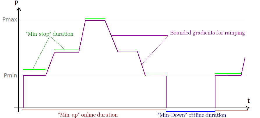
Figure 1: Illustration of the constraints for UCPd

To model possible power variations, three types of dynamic constraints are considered and illustrated Figure 1:

• Min-up/min-down constraints: every unit $u$ has a minimum up time $\Delta^{on}_{u}$ online and a minimum down time $\Delta^{off}_{u}$ offline similarly to (6) and (7).

• Transition constraints: When a unit generates at an operating point $i$ at period $t$, the allowable transitions for period $t+1$ are either to keep operating at point $i$ or to shift to a neighboring point $j\in\{i-1,i+1\}$.

• Min-stop ramping constraints on operating points: Once unit $u$ produces on point $i$, the power must be stabilized during $\Delta_{u,i}^{+}$ (resp. $\Delta_{u,i}^{-}$) time steps before reaching point $i+1$ (resp. $i-1$), as illustrated in Figure 2.

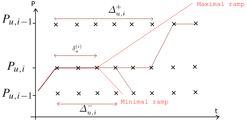
Figure 2: Illustration of the min-stop ramping constraints on the discretized operating points

3 Related work

ILP formulation results exist for min-up/min-down constraints. Takriti et al. (2000) provided a weak linear formulation with only set-up variables $x_{u,t}$, Lee et al. (2004) provided an exponential number of cuts to describe the convex hull of feasible integer points $x_{u,t}$ with a separation algorithm for a Branch&Cut implementation. Rajan and Takriti (2005) proved that (6) and (7) dominate the previous formulation and cuts and that the polytope defined with (2),(6),(7) and $0\leqslant x_{u,t},y_{u,t}\leqslant 1$ has integer extreme points. Rajan and Takriti (2005) showed in experimental results that the straightforward Branch&Bound resolution with (6) and (7) outperforms the Branch&Cut algorithm derived from Lee et al. (2004); Takriti et al. (2000).

A few decades ago, the solving capabilities of MILP solvers did not allow to consider realistic models of UC problems. MILP was widely used to model simple UC problems. With recent progress in the performances of computers and MILP solving, more realistic UC models are considered. Many works deal with additional dynamic constraints on thermal production. Arroyo and Carrion (2006); Morales-España et al. (2015) and Gentile et al. (2017) provided efficient MILP formulation to model start-up and shut-down trajectories when a thermal production is in the domain $[0,P_{u}^{min}]$. Silbernagl et al. (2016) and Brandenberg et al. (2017) provided efficient models to compute start-up costs and curves. Frangioni et al. (2008) presented different types and formulations for ramping constraints when a thermal production is in the domain $[P_{u}^{min},P_{u}^{max}]$, ensuring physical modulation constraints. Frangioni et al. (2009) presented MILP formulations for the ramping constraints. These formulations have been strengthened with the addition of start-up and shut-down variables by Ostrowski et al. (2012) and Damcı-Kurt et al. (2016). Correa-Posada et al. (2017) provided recently more realistic formulations of ramping constraints.

UC problems consider mostly a continuous production domain. The discretization is considered for the French case study, Dubost et al. (2005) solved a short term UC considering the whole French fleet with a Lagrangian approach dualizing demand constraints. Each thermal unit induces a sub-problem after dualization. The discretization allows to solve these sub-problems independently with dynamic programming. Kruber et al. (2018) added constraints in the dynamic programming algorithm to solve thermal sub-problems. We note that the influence of the discretization of ramping constraints and the relaxation transition phases was studied by Morales-España et al. (2017).

Formerly, MILP models of UC problems were commonly solved with Lagrangian decomposition dualizing demand constraints. Cheng et al. (2000) and Dubost et al. (2005) developed to Lagrangian heuristics. D-W decomposition dualizing demand constraints are similar and allow to compute Lagrangian bounds. Fu et al. (2005) and Rozenknopf et al. (2013) investigated D-W decomposition and Column Generation (CG) for long term UC problems.

4 Compact ILP formulation

Several variants to define the variables of UCPd can be considered. Several compact formulations of some constraints are also possible once variables are defined. Dupin (2017) used projections and isomorphisms to transform and compare the polyhedrons defined by compact ILP formulations. We present below one of the tightest ILP formulation provided by this work.

The production decisions are modeled using state variables $s_{u,t}^{(i)}\in\{0,1\}$ are defined with $s_{u,t}^{(i)}=1$ if and only if the unit $u\in\mathcal{U}$ operates exactly at the point $i\in\mathcal{I}_{u}$ and period $t\in\mathcal{T}$, else $s_{u,t}^{(i)}=0$.

To have the tightest compact and linear formulation, additional variables are considered similarly to Rajan and Takriti (2005). Start-up variables $y_{u,t}^{(i)-},y_{u,t}^{(i)+}\in\{0,1\}$ are defined for all $(u,t)\in\mathcal{U}\times\mathcal{T}$, and $i\in\mathcal{I}_{u}\cup\{0\}$ to indicate if unit $u$ is ramped up (resp. ramped down) to point $i$ at time $t$ from point $i-1$ (resp. from point $i+1$) at time $t-1$. Start-up variables are related with state variables: $y_{u,t}^{(i)+}=s_{u,t}^{(i)}.s_{u,t-1}^{(i-1)}$, $y_{u,t}^{(i)-}=s_{u,t}^{(i)}.s_{u,t-1}^{(i+1)}$.

To simplify the presentation of constraints, we extend the notations with $y_{u,t}^{(0)+}=y_{u,t}^{(N_{u}-)}=0$ for all $t$. The initial conditions are also considered with variables $s_{u,t}^{(i)},y_{u,t}^{(i)-},y_{u,t}^{(i)+}$ for $t\leqslant 0$ coding the previous production levels and moves.

It leads to the following ILP formulation:

$$\displaystyle\min_{s,y} \displaystyle\sum_{i}\left(C_{u}^{P}P(u,i)+C_{u}^{F}\right)s_{u,t}^{(i)}+\sum_{u,t}C_{u}^{S}y_{u,t}^{(1)+}$$ (8)

$$\forall u,t, \sum_{i}s_{u,t}^{(i)}\leqslant 1$$ (9)

$$\forall u,t,i, y_{u,t}^{(i-1)-}+\sum_{j\geqslant i}\left(s_{u,t}^{(j)}-s_{u,t-1}^{(j)}\right)=y_{u,t}^{(i)+}$$ (10)

$$\forall u,t,i, \sum_{j\geqslant i}s_{u,t}^{(j)}\leqslant\sum_{j\geqslant i-1}s_{u,t+1}^{(j)}$$ (11)

$$\forall u,t,i, \sum_{j\geqslant i}s_{u,t}^{(j)}\geqslant\sum_{j\geqslant i+1}s_{u,t+1}^{(j)}$$ (12)

$$\forall u,t,i, \sum_{t^{\prime}=t+1}^{t+\Delta_{u,i}^{+}}y_{u,t^{\prime}}^{(i+1)+}+\sum_{t^{\prime}=t+1}^{t+\Delta_{u,i}^{-}}y_{u,t^{\prime}}^{(i-1)-}\leqslant s_{u,t}^{(i)}$$ (13)

$$\forall u,t, \sum_{t^{\prime}=t-\Delta_{u}^{on}+1}^{t}y_{u,t^{\prime}}^{(1)+}\leqslant\sum_{i>0}s_{u,t}^{(i)}$$ (14)

$$\forall u,t, \sum_{t^{\prime}=t-\Delta_{u}^{off}+1}^{t}y_{u,t^{\prime}}^{(1)+}\leqslant 1-\sum_{i>0}s_{u,t-\Delta_{u}^{off}+1}^{(i)}$$ (15)

$$\forall t, \sum_{u,i}P(u,i)\phantom{1}s_{u,t}^{(i)}\geqslant D_{t}^{P}$$ (16)

$$\forall t, \sum_{u,i}R_{1}(u,i)\phantom{1}s_{u,t}^{(i)}\geqslant D_{t}^{R1}$$ (17)

$$\forall t, \sum_{u,i}R_{2}(u,i)\phantom{1}s_{u,t}^{(i)}\geqslant D_{t}^{R2}$$ (18)

Constraints (9) are implied by the definition of variables $s$: for all time period $t$, a unit $u$ produces at one operating point $i>0$ or is offline. Constraints (10) linearize the coupling constraints $y_{u,t}^{(i)+}=s_{u,t}^{(i)}.s_{u,t-1}^{(i-1)}$, $y_{u,t}^{(i)-}=s_{u,t}^{(i)}.s_{u,t-1}^{(i+1)}$. The tightest formulation of transition constraints and the min-stop ramping constraints. are respectively (11)-(12) and (13), we refer to Dupin (2017). Constraints (14) and (15) are the min-up/min-down constraints similarly to (6) and (7), noticing that the set-up and start-up variables $x_{u,t},y_{u,t}$ are $x_{u,t}=\sum_{i>0}s_{u,t}^{(i)}$ and $y_{u,t}=y_{u,t}^{(1)+}$. Constraints (16-18) are demand constraints in generated power, primary and secondary reserves.

5 Extended ILP formulation

This section investigates the D-W reformulation of previous ILP model, dualizing the demand constraints in power and reserves (Vanderbeck (2000)). The extended ILP formulation is presented with the Column Generation (CG) algorithm to solve its LP relaxation.

5.1 Extended ILP formulation

We denote by ${\mathcal{P}}^{u}$ the set of all the feasible production planning for unit $u$ considering the initial conditions and the technical constraints (9-15).

The variables of the extended formulation are indexed by ${\mathcal{P}}=\bigcup_{u}{\mathcal{P}}^{u}$, the set of all the possible production plannings. Binaries $z_{p}\in\{0,1\}$ are equal to $1$ if and only if the production planning $p\in{\mathcal{P}}$ is used in the global production planning. For each $p\in{\mathcal{P}}$, we denote by $P_{p,t}$, $R^{1}_{p,t}$, $R^{2}_{p,t}$ the production and reserves generated in the planning $p$ at period $t$. It gives rise to the following ILP formulation:

$$\min_{z_{p}\in\{0,1\}} \sum_{p\in{\mathcal{P}}}c_{p}z_{p}$$ (19)

$$\forall t\in{\mathcal{T}},\phantom{2} \sum_{p\in{\mathcal{P}}}P_{p,t}z_{p}\geqslant D_{t}^{P}$$ (20)

$$\forall t\in{\mathcal{T}},\phantom{2} \sum_{p\in{\mathcal{P}}}R^{1}_{p,t}z_{p}\geqslant D_{t}^{R1}$$ (21)

$$\forall t\in{\mathcal{T}},\phantom{2} \sum_{p\in{\mathcal{P}}}R^{2}_{p,t}z_{p}\geqslant D_{t}^{R2}$$ (22)

$$\forall u\in{\mathcal{U}},\phantom{2} \sum_{p\in{\mathcal{P}}_{u}}z_{p}=1$$ (23)

Constraints (20-22) are the demands in generated power and reserve capacities. Constraints (23) is required to express that a single production planning is assigned to each unit.

The dynamic constraints are induced in the definition of production patters ${\mathcal{P}}$. It is polyhedrally equivalent to consider the convex hull of the integer points defined by constraints (9-15). The LP relaxation of the extended formulation furnishes Lagrangian bounds, these dual bounds are at least as good as the LP relaxation of the compact ILP formulations (we refer to Vanderbeck (2000)).

The difficulty to deal with this formulation is that the set of feasible plannings has an exponential size and can be enumerated only for very small instances. Hence, CG techniques are required to deal with a reasonable number of variables.

5.2 Column Generation scheme

The LP relaxation of (19-23) is solved by the CG algorithm, adding iteratively new production patterns. Having a subset of production patters ${\mathcal{P}}^{o}\subset{\mathcal{P}}$, the Restricted Master Problem (RMP) denotes the LP relaxation of the previous ILP formulation restricted to the variables indexed by ${\mathcal{P}}^{o}$. Defining ${\mathcal{P}}_{u}^{o}={\mathcal{P}}_{u}\cap{\mathcal{P}}^{o}$, the RMP is written as following with the dual variables:

$$\begin{array}[]{lll}\mbox{RMP}({\mathcal{P}}^{o})&=\displaystyle\min_{z_{p}\geqslant 0}\displaystyle\sum_{p\in{\mathcal{P}}^{o}}c_{p}z_{p}\\ \forall t\in{\mathcal{T}},&\displaystyle\sum_{p\in{\mathcal{P}}^{o}}P_{p,t}z_{p}\geqslant D_{t}^{P}&\left(\pi^{P}\right)\\ \forall t\in{\mathcal{T}},&\displaystyle\sum_{p\in{\mathcal{P}}^{o}}R^{1}_{p,t}z_{p}\geqslant D_{t}^{R1}&\left(\pi^{R1}\right)\\ \forall t\in{\mathcal{T}},&\displaystyle\sum_{p\in{\mathcal{P}}^{o}}R^{2}_{p,t}z_{p}\geqslant D_{t}^{R2}&\left(\pi^{R2}\right)\\ \forall u\in{\mathcal{U}},&\displaystyle\sum_{p\in{\mathcal{P}}_{u}^{o}}z_{p}=1&(\sigma)\\ \forall p\in{\mathcal{P}}^{o},&z_{p}\geqslant 0\end{array}$$ (24)

The constraints (23) imply $z_{p}\leqslant 1$ and thus the LP relaxation can be written using only positivity constraints $z_{p}\geqslant 0$. As is, there are no dual variables associated to constraints $z_{p}\leqslant 1$.

The reduced cost related to the variable $z_{p}$, denoted by $\mbox{RC}(z_{p})$, has following value :

$$\mbox{RC}(z_{p})=c_{p}+\sigma_{u}-\sum_{t}\left(\pi_{t}^{P}P_{p,t}+\pi_{t}^{R1}R^{1}_{p,t}+\pi_{t}^{R2}R^{2}_{p,t}\right)$$

where $u$ is such that $p\in{\mathcal{P}}_{u}$.

The CG algorithm iterates while there exist no columns $p\in{\mathcal{P}}$ such that $\mbox{RC}(z_{p})<0$. In this case, $\mbox{RMP}({\mathcal{P}}^{o})$ is the value of the LP relaxation of (19-23). Otherwise, variables with a negative reduced cost are added in the RMP and the procedure is repeated till the stopping criterion is reached.

Solving $\mbox{RC}^{*}=\min_{p\in{\mathcal{P}}^{o}}\mbox{RC}(z_{p})$, the CG sub-problems, contains the two previous computations: $\mbox{RC}^{*}\geqslant 0$ is equivalent to the termination criterion, and optimal solutions have a negative reduced cost when $\mbox{RC}^{*}<0$ and can be selected to add in the RMP for the next iteration.

Computations to optimality of $\mbox{RC}^{*}$ are useful only for the last iteration, to prove the termination of the CG algorithm. Otherwise, heuristics are useful to generate quickly columns with a negative reduced cost and also to spend less time solving sub-problems.

We note that the CG algorithm requires the feasibility of $\mbox{RMP}({\mathcal{P}}^{o})$ at each iteration for the computations of the dual variables for the following sub-problems. The CG algorithm shall be initialized with columns ensuring the feasibility. The feasibility is ensured for each iteration adding columns. Removing columns with a null value in the last RMP has no effect in the feasibility of the next RMP, it allows to deal with bounded sizes of RMP. A first initialization strategy is to consider for each unit its maximal and minimal production planning regarding the technical constraints and the initial conditions. Otherwise, a global feasible planning can be computed quickly with the heuristics described by Dupin and Talbi (2016).

5.3 Solving CG subproblems

The key point is to solve efficiently $\mbox{RC}^{*}=\min_{p\in{\mathcal{P}}}\mbox{RC}(z_{p})$. The optimization are decomposed for each unit, $\mbox{RC}^{*}=\min_{u}\mbox{RC}^{*}_{u}$, where $\mbox{RC}^{*}_{u}=\min_{p\in{\mathcal{P}}_{u}}\mbox{RC}(z_{p})$ is the minimization problem over the feasible production patterns for unit $u$. Computations of $\mbox{RC}_{u}^{*}$ are independent and can be computed in parallel. It can be formulated using the compact ILP formulations of Section 4:

$$\mbox{RC}_{u}^{*}= \min_{x,y}f_{cout}^{u}(x,y)+f_{dual}^{u}(x)$$ (25)

$$\forall t, \sum_{i}x_{t}^{(i)}\leqslant 1$$ (26)

$$\forall t,i, \sum_{j\geqslant i}x_{t}^{(j)}\leqslant\sum_{j\geqslant i-1}x_{t+1}^{(j)}$$ (27)

$$\forall t,i, \sum_{j\geqslant i}x_{t}^{(j)}\geqslant\sum_{j\geqslant i+1}x_{t+1}^{(j)}$$ (28)

$$\forall t,i, y_{t}^{(i-1)-}+\sum_{j\geqslant i}\left(x_{t}^{(j)}-x_{t-1}^{(j)}\right)=y_{t}^{(i)+}$$ (29)

$$\forall t,i, \sum_{t^{\prime}=t+1}^{t+\Delta_{u,i}^{+}}y_{t^{\prime}}^{(i+1)+}+\sum_{t^{\prime}=t+1}^{t+\Delta_{u,i}^{-}}y_{t^{\prime}}^{(i-1)-}\leqslant x_{t}^{(i)}$$ (30)

$$\forall t, \sum_{t^{\prime}=t-\Delta_{u}^{on}+1}^{t}y_{t^{\prime}}^{(1)+}\leqslant\sum_{i>0}x_{t}^{(i)}$$ (31)

$$\forall t, \sum_{t^{\prime}=t-\Delta_{u}^{off}+1}^{t}y_{t^{\prime}}^{(1)+}\leqslant 1-\sum_{i>0}x_{t-\Delta_{u}^{off}+1}^{(i)}$$ (32)

$$\forall t,i, y_{t}^{(i)+},y_{t}^{(i)-},x_{t}^{(i}\in\{0,1\}$$ (33)

where the objective function is composed of $f_{cost}^{u}(x,y)$, the production costs like in the compact formulation, and $f_{dual}^{u}(x)$ are additional dual costs:

$\displaystyle f_{dual}^{u}(x)=\sigma_{u}-\sum_{u,i,t}\left(\pi^{P}_{t}P_{u,i}+\pi^{R1}_{t}R^{1}_{u,i}+\pi^{R2}_{t}R^{2}_{u,i}\right)\phantom{1}x_{t}^{(i)}$

$\displaystyle f_{cost}^{u}(x,y)=\sum_{t}\left(C^{F}_{u}x_{t}^{(1)}+C^{S}_{u}y_{t}^{(1)+}+\sum_{i}C^{P}_{u}P_{u,i}x_{t}^{(i)}\right)$

If $\mbox{RC}_{u}^{*}$ is written as an ILP, it can be computed with a dynamic programming algorithm, ensuring a polynomial complexity to the sub-problem resolution.

6 Experimental results

The computational experiments used the instance dataset from Dupin (2017). These instances were generated from real-world data for the French thermal fleet. Time horizon is $2$ days, with $96$ periods of $30$ minutes. There are up to $80$ generating units, with around $3$ discrete points per unit.

Tests were computed with an Intel(R) Core(TM) i5-4430 CPU, 3.00GHz, running Linux, with 4 CPU cores. ILP and LP were solved with Cplex 12.6 using the OPL interface as a first implementation. A first issue is to compare the quality of the LP relaxation of the extended formulation and the compact formulations from Dupin (2017), and to examine if LP relaxation improvements have a positive impact on the exact resolution. A second issue is to derive primal heuristics from the CG algorithm.

It is a known result that the LP relaxation with D-W reformulation is at least as good as the ones of compact formulations. More precisely, the D-W reformulation is equivalent to consider the convex hull of the polyhedron defined by the subproblems. The equality of both LP relaxations are reached when the polyhedrons defined by the sub-problems have integer extreme points in the compact formulation (Vanderbeck (2000)). The improvements of the LP relaxation provided by Dupin (2017) also tightened the sub-problems defined for each unit, which was a first way to close the gap between the first LP relaxation to the LP relaxation with a convexification of sub-problems. Actually, the LP relaxation of sections 4 and 5 have exactly the same value for each considered instance. These empirical results on the LP relaxation suggest to conjecture that the tightest compact formulations provide tight formulations for the min-stop ramping constraints:

Conjecture 1

The polytope defined for a single unit with constraints (26)-(32) describes the convex hull of the feasible integer points for the min-stop ramping constraints. In other words, the ILP formulation of constraints (26)-(32) is tight, and the Dantzig-Wolfe reformulation of UCPd dualizing demand and reserve constraints has the same LP relaxation than the compact formulation of section 4 and the other tightest and equivalent formulation derived by Dupin (2017).

Such conjecture generalizes the polyhedral results obtained by Rajan and Takriti (2005). This conjecture was verified computing sub-problems (26)-(32) as LP or ILP during CG iterations. Finding a counter-example where the LP relaxation and the ILP resolution of a CG sub-problem have different optimal values, this would induce that the conjecture is false. This was never observed, opening the perspective to prove formally the conjecture.

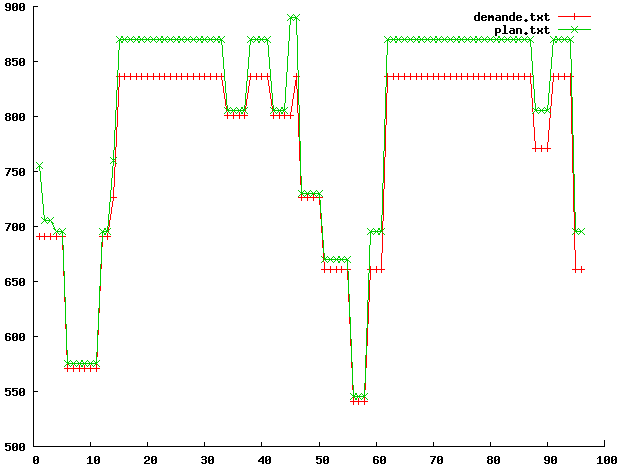
Figure 3: Demand covering with constraints (16)-(18)

We note that the convergence of the CG scheme is difficult, requiring much more time than compact LP relaxations. The dual variables are very unstable, with a erratic convergence. Indeed, for most of the iterations, the dual variables indexed by the time periods have few non-zeros. It tends to generate columns with peaks of production in the periods with non-zeros, and null productions where it is possible with the min-stop ramping and min-up/min-down constraints. This structure of dual variables is actually implied by the inequalities (16-18). Power discretization and the min-stop ramping constraints imply that few constraints (16-18) reach the lower bounds imposed by the constraints as illustrated in Figure 3. The complementary slackness theorem ensures that the corresponding dual variables of the non-saturated constraints are null. Such types of production planning given by the CG iterations are not efficient to be combined in global and feasible integer solutions. This closes the perspectives to use CG iterations for a primal heuristic based on the integer RMP and CG iterations, and validates also the matheuristics from Dupin and Talbi (2018).

These results validate to use in practice compact ILP formulations for UCPd, in a Branch&Bound resolution and in the computation of LP relaxation for the LP-based heuristics from Dupin and Talbi (2018). These results for UCPd are specific to this simple UC model. Modeling constraints (16) as inequalities induced difficulties for the convergence of the CG algorithm, whereas the minimization of the slackness to the power demands like in Goal Programming approaches would be more convenient for a CG scheme and CG heuristics. Lastly, a gap between compact LP relaxations and convexified extended formulations shall be analyzed considering in the UC model other types of power plants and/or more realistic constraints for thermal power plants, like in the work of Rottner (2018).

References

- Arroyo and Carrion (2006) Arroyo, J. and Carrion, M. (2006). A computationally efficient mixed-integer linear formulation for the thermal unit commitment problem. IEEE Transactions on power systems, 21(3), 1371 – 1378.
- Brandenberg et al. (2017) Brandenberg, R., Huber, M., and Silbernagl, M. (2017). The summed start-up costs in a unit commitment problem. EURO Journal on Computational Optimization, 5(1), 203–238.
- Cheng et al. (2000) Cheng, C.P., Liu, C.W., and Liu, C.C. (2000). Unit commitment by lagrangian relaxation and genetic algorithms. IEEE Transactions on Power Systems, 15(2), 707–714.
- Correa-Posada et al. (2017) Correa-Posada, C., Morales-España, G., Dueñas, P., and Sánchez-Martín, P. (2017). Dynamic ramping model including intraperiod ramp-rate changes in unit commitment. IEEE Transactions on Sustainable Energy, 8(1), 43–50.
- Damcı-Kurt et al. (2016) Damcı-Kurt, P., Küçükyavuz, S., Rajan, D., and Atamtürk, A. (2016). A polyhedral study of production ramping. Mathematical Programming, 158(1), 175–205.
- Dubost et al. (2005) Dubost, L., Gonzalez, R., and Lemaréchal, C. (2005). A primal-proximal heuristic applied to the French Unit-commitment problem. Mathematical Programming, 104(1), 129–151.
- Dupin (2015) Dupin, N. (2015). Modélisation et résolution de grands problèmes stochastiques combinatoires: application à la gestion de production d’électricité. Ph.D. thesis, Lille 1.
- Dupin (2017) Dupin, N. (2017). Tighter MIP formulations for the discretised unit commitment problem with min-stop ramping constraints. EURO Journal on Computational Optimization, 5(1), 149–176.
- Dupin and Talbi (2018) Dupin, N. and Talbi, E. (2018). Parallel matheuristics for the discrete unit commitment problem with min-stop ramping constraints. International Transactions in Operational Research, In press, available online, 1–25.
- Dupin and Talbi (2016) Dupin, N. and Talbi, E.G. (2016). Matheuristics for the discrete unit commitment problem with min-stop ramping constraints. Matheuristics 2016, 72–81.
- Frangioni et al. (2008) Frangioni, A., Gentile, C., and Lacalandra, F. (2008). Solving unit commitment problems with general ramp constraints. Journal of Electrical Power&Energy Systems, 30(5), 316–326.
- Frangioni et al. (2009) Frangioni, A., Gentile, C., and Lacalandra, F. (2009). Tighter approximated MILP formulations for unit commitment problems. IEEE Transactions on Power Systems, 24(1), 105–113.
- Fu et al. (2005) Fu, Y., Shahidehpour, M., and Li, Z. (2005). Long-term security-constrained unit commitment: hybrid Dantzig-Wolfe decomposition and subgradient approach. IEEE Transactions on Power Systems, 20(4), 2093–2106.
- Gentile et al. (2017) Gentile, C., Morales-Espana, G., and Ramos, A. (2017). A tight MIP formulation of the unit commitment problem with start-up and shut-down constraints. EURO Journal on Computational Optimization, 5(1), 177–201.
- Kruber et al. (2018) Kruber, M., Parmentier, A., and Benchimol, P. (2018). Resource constrained shortest path algorithm for EDF short-term thermal production planning problem. arXiv preprint arXiv:1809.00548.
- Lee et al. (2004) Lee, J., Leung, J., and Margot, F. (2004). Min-up/Min-down Polytopes. Discrete Optimization, 1, 77–85.
- Morales-España et al. (2015) Morales-España, G., Gentile, C., and Ramos, A. (2015). Tight MIP formulations of the power-based unit commitment problem. OR Spectrum, 37(4), 929–950.
- Morales-España et al. (2017) Morales-España, G., Ramírez-Elizondo, L., and Hobbs, B. (2017). Hidden power system inflexibilities imposed by traditional unit commitment formulations. Applied Energy, 191, 223–238.
- Ostrowski et al. (2012) Ostrowski, J., Anjos, M., and Vannelli, A. (2012). Tight mixed integer linear programming formulations for the unit commitment problem. IEEE Transactions on Power Systems, 27, 39–46.
- Rajan and Takriti (2005) Rajan, D. and Takriti, S. (2005). Min-Up/Down Polytopes of the Unit Commitment Problem with Start-Up Costs. Technical report, IBM Research Report.
- Renaud (1993) Renaud, A. (1993). Daily generation management at Electricité de France: from planning towards real time. IEEE Transactions on Automatic Control, 38(7), 1080–1093.
- Rottner (2018) Rottner, C. (2018). Combinatorial Aspects of the Unit Commitment Problem. Ph.D. thesis, Sorbonne Université.
- Rozenknopf et al. (2013) Rozenknopf, A., Calvo, R.W., Alfandari, L., Chemla, D., and Létocart, L. (2013). Solving the electricity production planning problem by a column generation based heuristic. Journal of Scheduling, 16(6), 585–604.
- Silbernagl et al. (2016) Silbernagl, M., Huber, M., and Brandenberg, R. (2016). Improving accuracy and efficiency of start-up cost formulations in MIP unit commitment by modeling power plant temperatures. IEEE Transactions on Power Systems, 31(4), 2578–2586.
- Takriti et al. (2000) Takriti, S., Krasenbrink, B., and Wu, L. (2000). Incorporating fuel constraints and electricity spot prices into the stochastic unit commitment problem. Operations Research, 48(2), 268–280.
- Vanderbeck (2000) Vanderbeck, F. (2000). On Dantzig-Wolfe decomposition in integer programming and ways to perform branching in a branch-and-price algorithm. Operations Research, 48(1), 111–128.