Gravitational Waves from merging binaries

Abstract

We discuss gravitational waves from merging binaries using a Newtonian approach with some inputs from the Post-Newtonian formalism. We show that it is possible to understand the key features of the signal using fundamental physics and also demonstrate that an approximate calculation gives us the correct order of magnitude estimate of the parameters describing the merging binary system. We build on this analysis to understand the range for different types of sources for given detector sensitivity. We also consider known binary pulsar systems and discuss the expected gravitational wave signal from these.

Jahanvi is an MS student at IISER Mohali. Her research interest is in Black-hole astronomy.

Ashish is a research scholar at IISER Mohali. His research interest is in gravitational lensing.

Jasjeet works at IISER Mohali. He is interested in diverse problems in physics, his research is in cosmology and galaxy formation.

June 2019 GENERAL ARTICLE

1 Introduction

Einstein introduced the general theory of relativity about $100$ years ago, and since then, scientists have validated its applicability in many ways via different experiments and observations [1, 2]. One of these tests is the loss of energy due to the emission of gravitational waves in a binary system. This was observed in the Hulse-Taylor binary by measuring the change in the semi-major axis and other orbital parameters over several decades [3, 4]. The gravitational waves distort the space-time curvature as they propagate. However, the amplitude of these distortions is very small [5, 6, 7, 8]. Hence the direct detection of gravitational waves was a major challenge for astronomers. Extremely sensitive detectors are required to detect gravitational waves and it took nearly four decades from initial concept to detection as considerable work had to be done in order to improve the sensitivity of the detectors [9, 10, 11].

The effort for direct detection of these gravitational waves started more than fifty years ago [12, 13, 14]. The gravitational waves were detected for the first time in $2015$ by LIGO (Laser Interferometer Gravitational-Wave Observatory) [15] from a merging black hole binary system. Up to second observing run (O2), a total of $11$ gravitational wave signals have been detected by LIGO. Out of these eleven signal, ten were from the merger of binary black holes, and one from a binary neutron star merger. The estimated mass of these black holes lies in a range $5$ M_⊙ to $60$ M_⊙.

With the increase in sensitivity of LIGO in the ongoing run and new detectors (KAGRA, INDIGO, LISA) [16, 17, 18, 19], the number of observed gravitational wave signals are expected to increase significantly. At the same time, we expect a more precise measurement of the source parameters for many sources. The detections of the gravitational wave signal provide a strong test for theories of gravitation in the regime of strong gravitational fields. More importantly, these detections open a new window for observing some of the most extreme events in the Universe. Among other things, gravitational wave astronomy is expected to help in probing the internal structure of neutron stars. Some of the events can also be used to study the expansion of the Universe [20].

In the current analysis, we discuss the possibility of detections of different mergers by LIGO/VIRGO or LISA (Laser Interferometer Space Antenna). We also discuss the prospects of detecting gravitational waves from known binary systems: Hulse-Taylor, and PSR J0737-3039 [21]. It turns out that at present PSR J0737-3039 is emitting gravitational waves in LISA frequency band whereas the value of the gravitational wave frequency corresponding to Hulse-Taylor binary is smaller than the LISA range. As this article is written from a pedagogical perspective, in order to calculate the required quantities, we use Newtonian approximation with some inputs from post-Newtonian corrections. The idea is to get an order of magnitude estimates while avoiding complications as much as possible. We also assume that the binary components are spin-less.

In §2, we present the mathematical formulae required for our current analysis. §3 contains a discussion of different types of mergers and the possibility of their detection. §4 includes a brief discussion of known binary systems. We summarize the discussion of gravitational waves from binary mergers in §5.

2 Gravitational waves emission

In this section, we set out our approach for relating the source parameters with the gravitational wave signal.

2.1 Keplerian Motion of a Binary System

The energy carried away by gravitational waves as a fraction of the total energy of the system is significant only at the time of the merger. In such a scenario, we can use Newton’s laws and Keplerian orbits to give an approximate description of the relation between the time period and the semi-major axis. This is a good approximation before the merger (see figure 1 and 2 for an illustration), the only thing that this does not capture is the evolution of the orbital parameters due to the emission of gravitational waves. Kepler’s third law gives the period of the orbital motion $T$, as [22]

$$T^{2}=\frac{4\pi^{2}}{G}\frac{a^{3}}{(m_{1}+m_{2})},$$ (1)

where $a$ is the semi-major axis of the orbit and $\left(m_{1},m_{2}\right)$ are the masses of the two components of the binary system.

The orbital frequency corresponding to the binary is given by the formula,

$$f_{orb}=\frac{1}{T}=\frac{1}{2\pi}\sqrt{\frac{G(m_{1}+m_{2})}{a^{3}}}$$ (2)

Since, the frequency of emitted gravitational waves is twice the orbital frequency, the frequency of the outgoing gravitational waves is given by,  [23]

$$f_{gw}=2f_{orb}=\frac{1}{\pi}\sqrt{\frac{G(m_{1}+m_{2})}{a^{3}}}.$$ (3)

In the weak field limit, it can be shown that the gravitational waves propagate at the speed of light, are transverse in nature and like the electromagnetic waves these have two polarizations [5]. For binaries in circular orbits, the strain due to the two gravitational wave polarizations at a distance $R$ from the binary, under Newtonian approximation, is given as,

$$h_{+}\left(t\right) = -\frac{1}{R}\frac{4G^{2}}{c^{4}}\frac{m_{1}m_{2}}{a}\frac{(1+\cos^{2}\textit{i})}{2}\>\cos[2\pi f_{gw}\left(t-R/c\right)+2\phi_{0}],$$

$$h_{\times}\left(t\right) = -\frac{1}{R}\frac{4G^{2}}{c^{4}}\frac{m_{1}m_{2}}{a}\>\cos\textit{i}\>\sin[2\pi f_{gw}\left(t-R/c\right)+2\phi_{0}],$$ (4)

where $a$ is the radius of the orbit, $i$ is the angle between the orbital angular momentum vector of the binary and the observer’s line of sight, and $\phi_{0}$ is the initial phase at time $t=0$.

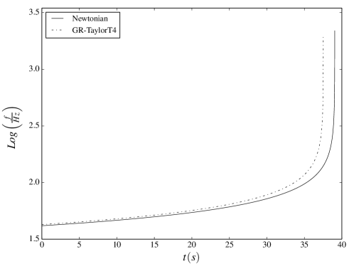
Figure 1: Time vs. frequency plot for a $1M_{\odot}+1M_{\odot}$ binary: The solid black line represents the frequency evolution of gravitational waves using equation (7). The dashed-dotted line is the frequency evolution under the Taylor-T4 approximant. The time $t=0$ corresponds to the stage where the semi-major axis is $250$ km.

Clearly, there is a loss of energy due to the emission of gravitational waves but this is not taken into account in our discussion of orbital parameters. At early times the orbital parameters vary at a very slow rate and the above relations can be applied over multiple orbits. At late stages, the change in orbital parameters is relatively rapid, and these relations should be thought of as instantaneous. It is noteworthy that strain is proportional to $1/R$. Hence, if our sensitivity for strain measurement improves by a factor, the range up to which we can observe events also increases by the same factor.

In order to establish that this approximation is reasonable for the quantities of interest in our discussion, we give the formulae for change of orbital parameters from leading order corrections of post-Newtonian (PN) calculations and provide a sample calculation.

2.2 Effects of Gravitational Wave emission

If the energy and angular momentum carried away by the gravitational waves within the observation period are significant, then orbital parameters and hence the frequency and amplitude of the emitted waves vary within a few orbital time periods. For a binary with elliptical orbit, the average rate of change of the semi-major axis $\left(a\right)$ and eccentricity $\left(e\right)$ with the time is given as [27]

$$\left\langle\frac{da}{dt}\right\rangle = -\frac{64}{5}\frac{G^{3}m_{1}m_{2}(m_{1}+m_{2})}{c^{5}a^{3}(1-e^{2})^{7/2}}\left(1+\frac{73}{24}e^{2}+\frac{37}{96}e^{4}\right),$$ (5)

$$\left\langle\frac{de}{dt}\right\rangle = -\frac{304}{15}\frac{G^{3}m_{1}m_{2}(m_{1}+m_{2})}{c^{5}a^{4}(1-e^{2})^{5/2}}e\left(1+\frac{121}{304}e^{2}\right).$$ (6)

As one can see from equation (5) and (6), as the binary system evolves in time, the eccentricity of the orbit decreases at a faster rate than the semi-major axis. However, if an orbit is already circular, it remains circular. Hence from this point onwards, until mentioned, we will be focusing on circular orbits for binaries in order to simplify the treatment and eliminate one parameter from the discussion. The change in orbital parameters leads to a corresponding change in the amplitude and frequency of outgoing gravitational waves. Up to leading order, the variation of frequency of outgoing gravitational waves emitted is given as,

$$f_{gw}(t)=\frac{5^{3/8}c^{15/8}}{8\pi G^{5/8}}\frac{1}{\mathcal{M}^{5/8}}(t_{c}-t)^{-3/8},$$ (7)

where $t_{c}$ is the coalescence time (time at which the distance between the two binary bodies goes to zero i.e. $a(t_{c})=0$) and $\mathcal{M}$ is the chirp mass of the binary system. This is defined as

$$\mathcal{M}\equiv\frac{(m_{1}m_{2})^{3/5}}{(m_{1}+m_{2})^{1/5}}.$$ (8)

Equation (7) implies that up to leading order the frequency of the outgoing gravitational waves at a time $t$ only depends on the chirp mass of the binary. In addition to this, at coalescence time, the frequency of outgoing gravitational waves goes to infinity, which indicates the failure of the leading order approximation. To get rid of this diverging behavior of frequency, one has to take into account the PN corrections. Figure  1, represents the frequency evolution for a $1M_{\odot}+1M_{\odot}$ circular binary. At the initial time, the orbital radius of the binary was taken to be $250$ km which is larger than the distance at the merger by more than a factor of 10. The solid line represents the frequency evolution under Newtonian approximation calculated using equation (7), whereas the dashed-dotted line represents the frequency evolution under general relativistic Taylor-T4 approximant [24], including post-Newtonian corrections. One can see that at the time of the merger, the frequency of emitted gravitational waves under Newtonian and the general relativistic approximation is of the same order. One can see from the figure 2, which represents the fractional change of frequency with time under Newtonian approximation, that long before the merger, the gravitational wave frequency evolves very slowly with time. However, as the system proceeds towards the merger phase, which lasts for a fraction of a second, the frequency of outgoing gravitational waves increase very rapidly. Here the maximum frequency represented in the figure  1 corresponds to the innermost stable circular orbit (ISCO) which is defined as $R_{ISCO}=6GM/c^{2}$ [8]. Looking at the figure, one can also observe that the maximum frequency of the outgoing gravitational waves lies in the LIGO frequency range.

The corresponding gravitational wave polarization functions are given as [8],

$$h_{+}(t) =\begin{aligned} &-\frac{4\pi^{2/3}(G\mathcal{M})^{5/3}}{c^{4}R}\frac{1+\cos^{2}\textit{i}}{2}\>f_{gw}^{2/3}\left(t\right)\\ &\qquad\qquad\quad\cos\left(2\pi\int_{0}^{t}f_{GW}\left(t^{\prime}\right)dt^{\prime}+2\phi_{0}\right)\end{aligned}$$ (9)

$$h_{\times}(t) =\begin{aligned} &-\frac{4\pi^{2/3}(G\mathcal{M})^{5/3}}{c^{4}R}f_{gw}^{2/3}\left(t\right)\cos\textit{i}\\ &\qquad\qquad\quad\sin\left(2\pi\int_{0}^{t}f_{GW}\left(t^{\prime}\right)dt^{\prime}+2\phi_{0}\right),\end{aligned}$$ (10)

where the symbols have their usual meaning. The above formulae can also be used for binaries at cosmological distances by replacing chirp mass $\mathcal{M}$ to $\left(1+z\right)\mathcal{M}$ and distance $R$ to luminosity distance to the binary. The current GW detectors can only observe binaries at redshifts less than one. Hence the effect of redshift will be introducing the uncertainty of factor two in the relevant quantities, at most. Keeping that in mind and for the simplicity of analysis, we drop the redshift dependent factor in our study.

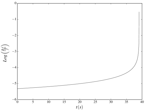
Figure 2: Time vs. fractional change in frequency of outgoing gravitational waves for a $1M_{\odot}+1M_{\odot}$ binary under Newtonian approximation (corresponding to figure  1).

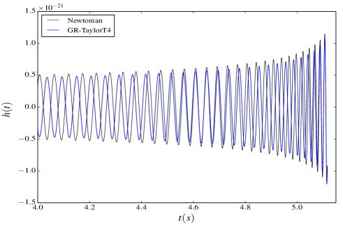
Figure 3: Comparison of Newtonian (equation (9) and (10)) and general relativistic chirp waveform: The black line shows the chirp waveform generated by using equation (9). The blue line is the waveform generated by using Taylor-T4 formula. The x-axis represents the time elapsed since the initial frequency $f=10\>Hz$. The y-axis represents the corresponding strain.

Figure 3 shows the chirp waveforms for a source binary which consists masses of $35.6\>M_{\odot}$ and $30.6\>M_{\odot}$ (similar to GW150914). The distance to the source binary is $430$ Mpc. The continuous black line is for the waveform generated under Newtonian approximations using equation (9) whereas the blue line represents the chirp waveform using general relativistic (Taylor-T4) approximations. The merging time for these two approximations is slightly different. Here, we manually aligned the waveform at the time of the merger to see the change in the frequency and amplitude in these two approximations close to the time of merger as these are the two quantities used in our analysis. One can see that the amplitude of strain in both approximations remains similar. That once again validates our idea of using Newtonian calculations to get an estimation for frequency and amplitude of the GW signal. However, the variation of the phase of the signal with time for these two approximations is different. We see that the estimation of amplitude is very good and the frequency at merger is correct to within about $10\%$. Thus, our use of a Newtonian approximation for orbits near the time of merger is justified.

3 Binary Systems

Gravitational-wave detectors are sensitive to a specific frequency bands. Hence, the possibility of detection of the gravitational waves coming from a source, binary depends on the frequency of gravitational waves. The maximum frequency of gravitational waves emitted from a binary depends on the parameters of the source binary. The detailed waveform is used to constrain the parameters of the source, though it is possible to get an estimate by using the the frequency at the time of the merger. In our discussion, we focus on the frequency at the time of the merger, since it can be estimated without complicated calculations, as we have shown in figure 1.

In the current section, we discuss different kinds of binary mergers which can be detected by LIGO or LISA. Binaries can have main sequence stars (MS), white dwarfs (WD), neutron stars (NS) or black holes (BH). These binaries can either consist of similar kind of components (NS-NS, BH-BH, MS-MS, WD-WD) or can be made of a different kind of binary components (NS-BH, NS-MS, NS-WD, WD-BH, WD-MS, and BH-MS). The prospects for detection depend on the detector sensitivity and the frequencies where gravitational waves can be detected. We consider different types of binaries in sub-sections below.

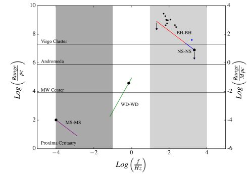
Figure 4: Frequency vs. range for same binary components: The range is computed assuming a strain value $10^{-21}$, i.e., the detector noise is well below this level. The light and dark gray regions represent the frequency band corresponding to LIGO and LISA. The horizontal lines mark some standard distances. The blue, red, green, violet lines represent the merger of NS-NS, BH-BH, WD-WD, MS-MS, respectively. The large filled black circles mark objects with a mass equal to that of the Sun. Small filled circles mark mergers observed by LIGO, black circles are for black holes, and the blue circle is for merging neutron stars. See text for more details.

3.1 Binaries With Similar Components

In order to limit the number of parameters, we first consider binaries made up of identical components. That is, both the components are of the same type and have the same mass. This is adequate for our purpose, and the reader can easily generalize this analysis using the formulae given below for any combination of masses. The gravitational waves have the highest frequency when the distance between the binary components is minimum. For MS and WD this corresponds to the stage when the objects are touching each other. In case of BH and NS this corresponds to the innermost stable circular orbit (ISCO). $R_{ISCO}$ for an object of mass $M$ is

$$R_{ISCO}=\frac{6GM}{c^{2}}$$ (11)

where symbols have their usual meaning.

For a BH-BH or NS-NS merger, this minimum distance is taken to be the sum of $R_{ISCO}$ for each object,

$$a_{min}=\frac{6G\left(m_{1}+m_{2}\right)}{c^{2}},$$ (12)

where $m_{1}$ and $m_{2}$ are masses of binary components. If at some initial time $t_{in}=0$, the distance between the binary components is $a_{in}$, then the time taken by the binary to reach the final stage $\left(a=a_{min}\right)$ can be calculated by integrating equation (5) as,

$$t_{m}=\frac{a_{in}^{4}-a_{min}^{4}}{4\beta},\,\,\,\,\,\,\beta=\frac{64}{5}\frac{G^{3}m_{1}m_{2}(m_{1}+m_{2})}{c^{5}}$$ (13)

From this equation, we see that the coalescence time is given as, $t_{c}=a_{in}^{4}/4\beta$.

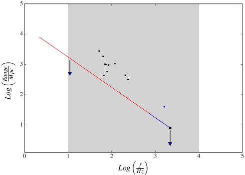
Figure 5: Frequency vs. range for same binary components in LIGO range: The blue line represents the NS-NS mergers and red line represents the BH-BH mergers with strain $10^{-21}$. The blue dot represents NS-NS merger and black dots represents BH-BH mergers observed by LIGO.

Figure 6: Peak frequency vs. range for different binary components: The axis labels are similar to that of figure 4. The light and dark gray regions represent the frequency band corresponding to LIGO and LISA. The horizontal lines mark some standard distances. The red, brown, violet lines represent the merger of Black hole with a neutron star, white dwarf and main-sequence star, respectively. Whereas the blue and green lines represent the merger of white dwarf and main-sequence star with a neutron star, respectively.

Hence from equation (3), for a BH-BH or NS-NS merger, the frequency of gravitational waves at $a=a_{min}$ is given as,

$$f_{gw}(t_{m})=\frac{1}{\pi}\sqrt{\frac{G(m_{1}+m_{2})}{a_{min}^{3}}}$$ (14)

The corresponding value of the range, from equation (4), can be given as

$$R=\frac{4G^{2}}{c^{4}}\frac{m_{1}m_{2}}{a_{min}}\frac{1+\cos^{2}\textit{i}}{2}\frac{1}{h(t_{m})},$$ (15)

where $h\left(t_{m}\right)$, is the observed value of strain at the merger time. We know from the equation (9) and (10) that the range value is inversely proportional to the detected strain of the GW signal. Hence, if LIGO detects a signal with strain value $10^{-22}$ ($10^{-20}$), then the corresponding range value will go up (down) by a factor of $10$ with respect to the range of strain value of $10^{-}21$. The sensitivity of LIGO and LISA is frequency-dependent. Hence, the strain threshold is frequency-dependent if we work with a given signal to noise ratio (SNR). We ignore this and fix the strain value to $10^{-21}$ to keep the analysis simple. However, we do provide a qualitative indication on how this affects the range, where relevant. The above formulae for calculating merger frequency and range are valid for all kinds of binaries only the values of $a_{min}$ are different for different binaries. Note that we are using equation  (3) and equation (4) for these calculations.

The mass-radius relation for a white dwarf is given as [25, 26],

$$R_{WD}\propto M_{WD}^{-1/3},$$ (16)

where $R$ is the radius and $M$ is the total mass of the white dwarf. This relation applies for white dwarfs with non-relativistic degenerate electron gas but we choose to extrapolate it to the Chandrasekhar mass limit. In order to fix the constant of proportionality, we take the radius for a solar mass white dwarf to be $6000$ km. Hence the minimum distance attained by a WD-WD binary with mass $(m_{1},m_{2})$ is given as

$$a_{min}=6000\>\mathrm{km}\left\{\left(\frac{M_{\odot}}{m_{1}}\right)^{1/3}+\left(\frac{M_{\odot}}{m_{2}}\right)^{1/3}\right\}$$ (17)

For a main-sequence star, the mass-radius relation is given as  [26]

$$R_{ms}\propto M_{ms}^{\alpha}$$ (18)

where $\alpha=0.8$ for a main-sequence stars with mass greater than $1M_{\odot}$ and $\alpha=1.0$ for stars with $0.08$ M$\odot\leq M\leq 1$ M_⊙. The minimum distance attained by an MS-MS binary with mass $\left(m_{1},m_{2}\right)$ is given as

$$a_{min}=R_{\odot}\left(\frac{m_{1}^{\alpha}}{M_{\odot}}+\frac{m_{2}^{\alpha}}{M_{\odot}}\right),$$ (19)

where $R_{\odot}$ is the radius of the Sun. The corresponding value of frequency and range at the time of the merger can be calculated by using equations (14) and (15). Figure 4 shows the merger of binaries with identical binary components with equal masses. The dark and light-shaded regions represent the frequency range corresponding to LISA and LIGO detectors. The x-axis represents the frequency of emitted gravitational waves at the time of the merger. The y-axis represents the range up to which a gravitational wave signal can be detected with a strain value of $10^{-21}$ by the detector. The LIGO detectors have a higher sensitivity so we can see mergers out to larger distances. Further, it has to be kept in mind that our estimates are based on an approximate analysis. The black horizontal lines mark some key distances. The red line marks the merger of binary black holes with the same masses from $3$ M_⊙ to $100$ M_⊙. Similarly, the blue line shows the merger of binary neutron stars with the mass in a range from $1$ M_⊙ to $3$ M_⊙. The black dot on the blue line represents the merger of a $1$ M${}_{\odot}+1$ M_⊙ neutron star binary. The black dots above the red line show the observed BH-BH mergers and the blue dot is for the observed neutron star merger. The frequencies are plotted in the source frame and not the observer frame for ease of comparison. One can see that LIGO can detect BH-BH as well as NS-NS mergers. The BH binaries are the most distant binaries that can be detected by LIGO. However, as we know from the noise curves for the LIGO detector that at the lower and higher end of the allowed frequency range, the noise level is higher than the middle of the frequency range. Hence, the signal to noise ratio (SNR) at these frequency values also goes down. As a result, the maximum distance up to which LIGO can detect a binary merger at these frequencies also decreases. Hence the observed range value will be smaller than the value predicted by using equation 15. This effect is denoted by downward arrows in figure 4. On the other hand, the main-sequence star binaries with component mass less than or equal to one solar mass can be detected by LISA, but the distances up to which these binaries can be detected are much smaller than the size of our own galaxy. Indeed, for the assumed sensitivity, we can only detect such mergers in the local neighborhood of the Sun within a radius of about a few hundred parsecs. The black dot on the violet line represents the merger of $1$ M${}_{\odot}+1$ M_⊙ main-sequence star binary. Mass of components is lower for the higher frequency at merger. Some white dwarf binaries with masses on the lower end ($0.1$ M_⊙) can be detected by LISA, but higher mass WD mergers cannot be detected by LISA or LIGO. The black dot on the green line marks the merger of a $1$ M${}_{\odot}+1$ M_⊙ white dwarf binary. Mass of WD is higher for the higher frequency at the merger.

Mergers in the frequency range of LIGO are also shown in figure 5 to focus on the relevant distance scale. The range for BH mergers is much higher than the range for NS mergers. This implies that we will be able to see many more BH mergers even though the expected rate of such mergers per galaxy is much smaller. This is because the volume within which we can see a merger of a given type scales as the cube of the range. We see that the distance to the detected BH mergers lies in a range from $100$ Mpc to $3000$ Mpc whereas the distance to NS binary is around $40$ Mpc. If we gradually increase the mass of black holes, the maximum frequency of gravitational waves decreases and moves towards the LISA range.

3.2 Binaries With Different Components

In this section, we explore mergers of dissimilar objects. This possibility includes the merger of BH-NS, BH-WD, BH-MS, NS-WD, NS-MS and WD-MS. We now use the sum of cutoff radius for each component to obtain the smallest distance that marks the merger: for MS and WD it is the sum of individual radii, and for NS and BH we take the radius of the innermost stable circular orbit. Thus for a WD-NS merger, we take the physical radius of the WD and add $R_{ISCO}$ for the NS to obtain the semi-major axis at the time of merger.

Figure 6, shows the prospects of detection of such mergers. As one can see LIGO can detect the merger of BH-NS, where we have assumed that the neutron star has a mass equal to the Sun, and the black hole has a mass in a range from $1-1000$ M_⊙. Again the downward arrows show the decrement in SNR (and the range value) at the lower and higher end of the LIGO frequency range. The merger of a sun-like star and a neutron star or a black hole can be detected by LISA but with a range that is limited to the local group for the assumed sensitivity. The merger of a white dwarf of one solar mass with a neutron star cannot be detected by LIGO or LISA. However, the merger of a white dwarf with a super-massive black hole can be detected by LISA.

As one can see from figure 4, 5 and 6, the neutron star and black hole mergers can be detected by LIGO but as we increase the mass of the black hole the maximum frequency of gravitational waves emitted by binary decreases and gradually moves towards the LISA domain.

Figure 7: Frequency vs. strain for observed binary systems: The light and dark gray regions represent the frequency band corresponding to LIGO and LISA. The two black dots represent the value of frequency and strain at the present time. The system evolves towards higher frequencies and higher strain amplitude.

4 Observed Binary Systems

In this section, we briefly take a look at the known binary systems, namely, PSR B1913+16 (Hulse-Taylor binary) and PSR J0737-3039. The Hulse-Taylor binary [4] consists of one pulsar along with a neutron star whereas in PSR J0737-3039, both components are pulsars.

The expected merger time for the two binaries is very large: $87$ Myr for PSR J0737-3039 and more than a Gyr for the Hulse-Taylor binary pulsar. Hence, the value of the frequency and amplitude of the emitted gravitational waves are very small. Figure 7, represents the change in frequency and strain for these two binary systems as they proceed towards their merger phase. The black dots represent the current value of frequency and strain for these binaries. As one can see, at present the frequency of outgoing gravitational waves from PSR J0737-3039 lies in the LISA range whereas the frequency for the Hulse-Taylor binary lies outside the LISA range. As expected for a neutron star binary, the frequency of emitted gravitational waves from Hulse-Taylor binary and PSR J0737-3039 at the time of merger lies in the LIGO band.

5 Conclusion

We discussed gravitational waves from mergers of different types. We have used a simple Newtonian analysis to understand key aspects of the expected signal. We are able to calculate the frequency and the range at merger using a Newtonian approach. Given the combination of the frequency and range, it is clear that LIGO can only detect binaries with BH and NS as its components. LISA will be able to detect other types of mergers but the ranges for these are relatively limited as MS and WD are less compact and the gravitational field at the time of merger is not as strong as in the case of BH and NS. The range is highest for mergers of black holes, and this is reflected in the more significant number of such events observed by LIGO so far.

It is interesting to note that LISA can detect gravitational waves coming from PSR J0737-3039. Observations from the square kilometer array (SKA) [28] may add to the list of such sources.

Unlike electromagnetic radiation, gravitational waves interact very weakly with matter, and therefore the information carried by it undergoes fewer modifications during propagation. As we have seen above all these signals are coming from binary mergers, these detections can help us to understand the processes during the merger of binary components which may not be seen otherwise.

If one of these binary components is a neutron star, the merger leads to the emission of electromagnetic radiation as well, as seen in GW170817. More such sources will be discovered in the ongoing and future runs of LIGO. The combined analysis of gravitational waves and electromagnetic radiation can help us in constraining the theories that describe the structure of neutron stars and properties of matter at very high densities, as well as cosmological parameters.

References

- [1] Will C. M., 2010, AmJPh, 78, 1240
- [2] Weinberg S., 1972, Gravitation and Cosmology: Principles and Applications of the General Theory of Relativity. Wiley-VCH.
- [3] Taylor J. H., 1993, CQGra, 10, S167
- [4] Weisberg J. M., Taylor J. H., 2005, ASPC..328, 25, ASPC..328
- [5] Biman Nath, 2016, Resonance, 21, 3, 213-224.
- [6] Thorne K. S., 1997, arXiv e-prints, gr–qc/9704042
- [7] Schutz B., 2009, A First Course in General Relativity by Bernard Schutz. Cambridge University Press.
- [8] Maggiore M., 2009, Gravitational Waves: vol. 1: Theory and Experiments. Oxford University Press.
- [9] Weiss, Rainer, 2018, Rev. Mod. Phys., 90, 4, 040501.
- [10] Barish, Barry C., 2018, Rev. Mod. Phys., 90, 4, 040502.
- [11] Thorne, Kip S., 2018, Rev. Mod. Phys., 90, 4, 040503.
- [12] Weber, J., 1969,Phys. Rev. Lett., 22, 24, 1320–1324
- [13] Weiss, R., MIT, Quarterly Progress Report, No. 105, 1972 (available at https://dcc.ligo.org/public/0038/P720002/001/qpr1972.pdf)
- [14] Press W. H., Thorne Kip S. 1972, Annual Revs. Astron. Astroph. 10, 335–374
- [15] The LIGO Scientific Collaboration, et al., 2018, arXiv e-prints, arXiv:1811.12907
- [16] KAGRA Collaboration, 2018, Progress of Theoretical and Experimental Physics, 2018
- [17] Souradeep T., 2016, Resonance. 21, 3, 225-231.
-
[18]
Iyer, B., et al. 2011 , LIGO-DCC, LIGO-India, Tech. Rep. LIGO-M1100296,
https://dcc.ligo.org/LIGO-M1100296/public - [19] Amaro-Seoane P., et al., 2012, CQGra, 29, 124016.
- [20] Ajith P., Arun K. G., 2011, Resonance, 16, 10, 922-932.
- [21] Kramer, M. and Stairs, I.H., 2008, Annual Review of Astronomy and Astrophysics, 46, 1, 541-572
- [22] Zeilik M., Gregory Stephan A., 1998, Introductory Astronomy and Astrophysics, 4th Edition, Thomson Learning.
- [23] Carroll S. M., 2004, Spacetime and Geometry: An Introduction to General Relativity.
- [24] Boyle, Michael et. al., 2007, Phys. Rev. D, 76, 12, 124038.
- [25] Chandrasekhar S. 1939, An introduction to the study of stellar structure, Chicago University Press.
- [26] Prialnik D., 2010, An Introduction to the Theory of Stellar Structure and Evolution, 2nd Edition. Cambridge University Press.
- [27] Peters, P. C., 1964, Phys. Rev., 136, 4B, B1224–B1232
- [28] Huynh, M., Lazio, J., 2013, arXiv e-prints, 1311.4288.