Neural Networks Weights Quantization: Target None-retraining Ternary (TNT)

Abstract

Quantization of weights of deep neural networks (DNN) has proven to be an effective solution for the purpose of implementing DNNs on edge devices such as mobiles, ASICs and FPGAs, because they have no sufficient resources to support computation involving millions of high precision weights and multiply-accumulate operations. This paper proposes a novel method to compress vectors of high precision weights of DNNs to ternary vectors, namely a cosine similarity based target non-retraining ternary (TNT) compression method. Our method leverages cosine similarity instead of Euclidean distances as commonly used in the literature and succeeds in reducing the size of the search space to find optimal ternary vectors from $3^{N}$ to $N$, where $N$ is the dimension of target vectors. As a result, the computational complexity for TNT to find theoretically optimal ternary vectors is only $O(N\log(N))$. Moreover, our experiments show that, when we ternarize models of DNN with high precision parameters, the obtained quantized models can exhibit sufficiently high accuracy so that re-training models is not necessary.

1 Introduction

Quantizing deep neural networks (DNNs) can reduce memory requirements and energy consumption when deploying inferences on edge devices, such as mobiles, ASICs and FPGAs. Comparing with networks quantized by other methods, the binary and ternary networks use only $1$ or $2$ bits to represent DNNs’ weights, and therefore, can further improve the performance of inferences of DNN on edge devices because they not only remove multiplication operations but use less memory as well. As a result, many researches focus on binary and ternary quantifications.

BinaryConnect[1] proposed a sign function to binarize the weights. Binary Weight Network (BWN) [2] introduced the same binarization function but added an extra scaling factor to obtain better results. BinaryNet [3] and XNOR-Net [2] extended the previous works so that both weights and activations were binarized. Instead of binarization, ternarization, which inherently prunes weights close to zero by setting them to zero during training to make networks sparser, is further studied. TWN [4] quantized full precision weights to ternary weights so that the Euclidean distance (Second Normal Form) between the full precision weights and the resulting ternary weights along with a scaling factor is minimized. GXNOR-Net [5] provided a unified discretization framework for both weights and activations. Alemdar et al. [6] trained ternary neural networks using a teacher-student approach based on a layer-wise greedy method. Mellempudi et al. [7] proposed a fine-grained quantization (FGQ) to ternarize pre-trained full precision models, while also constraining activations to 8 and 4 bits.

The parts in inference computation that consume time and energy in the largest scale involve many weights in computation, which are saved as tensors in every layer. A tensor can be decomposed to a set of vectors, referred to as target vectors, and each target vector is approximated to a binary or ternary vector. To control the approximation error, Euclidean distance is the most commonly utilized in many previous works in: these quantization methods measure the approximation error or similarity between original target vectors and the approximated ternary or binary vectors as Euclidean distances. This method, however, is known to require expensive computation. For example, the time complexity of the tenary method proposed in [7] was $O(N^{3})$. In this paper, we propose a novel tenary method whose time complexity is improved to $O(N\log N)$ by replacing Euclidean distance by cosine similarity. We call our method a cosine similarity based target non-retraining ternary (TNT) method. In addition, our method has following advantages: 1) TNT is a non-retraining optimal quantization method for ternarization, binarization, and low bit-width quantizations; 2) We find the theoretical upper limit of similarity between target vectors and ternary vectors; it is guaranteed that TNT always finds the optimal ternary vectors with the maximum similarity of original vectors; 3) We find the similarity is influenced by distributions of component values of target vectors, and furthermore, higher similarity can be obtained if we assume uniform distributions than normal distributions.

2 Method Description

The proposed TNT first divides the tensor type weights of a DNN model into plural target vectors. Then, it finds the ternary vector most similar to every target vector with respect to cosine similarity. In other words, the ternary vector is selected so that the intersection angle between the target vector and ternary vector is minimized. Finally, it uses a scalar-tuning technique to adjust the error between one target vector and its ternary vector to obtain an optimal converting result.

2.1 Tensor Decomposition and Vectorization

The weights of a DNN are normally stored in a fourth-order tensor shape, such as $N\times C\times W\times H$, that contains $N$ third-order tensors and every third-order tensor has $C$ channels, $W$ width, and $H$ height. The purpose of tensor vectorization is to flatten every third-order tensor into a set of target vectors. We expect that decomposing a tensor along the channel direction can yield good results, because each channel is an integral unit which acts as a feature extractor for convolution calculations with a feature map. Hence, a third-order tensor can be vectorized to $\mathcal{W}^{(1)},\mathcal{W}^{(2)},\cdots,\mathcal{W}^{(C)}$. This expectation will be verified through experiments in this paper.

2.2 Target Non-retrain Ternarization

We first introduce our cosine similarity based technique TNT, which reduces the searching range to $N$. Then, a scalar-tuning method is proposed to further optimize the ternary vector. The total of the computational complexity is $O(N\log N)$.

2.2.1 Cosine Similarity

Given a target vector of a layer $j$ of a CNN, which is denoted by $\bm{w}^{(j)}=(w_{1}^{(j)},\cdots,w_{N}^{(j)})$ for $w_{i}^{(j)}\in\mathbb{R}$, the purpose is to find a ternary vector $\bm{t}^{(j)}=(t_{1}^{(j)},\cdots,t_{n}^{(j)}),t_{i}^{(j)}\in\{-1,0,1\}$ that approximates $\bm{w}^{(j)}$. For simple representation of equations, we eliminate the notation of $j$ since it only represents a layer $j$. In TNT, we use the cosine similarity metric between the two vectors to find the optimal ternary vector $\bm{t}$. The cosine similarity between the target vector $\bm{w}$ and the ternary vector $\bm{t}$ can be written as Eq.(1), where $\bm{\widehat{w}}=\frac{\bm{w}}{\|\bm{w}\|_{2}}$ and $\alpha\in[0,\pi)$ is the intersecting angle between $\bm{w}$ and $\bm{t}$. The value of $\cos\alpha$ is controlled by vector $\bm{t}$ since every element $w_{i}$ in the target vector $\bm{w}$ is fixed.

$$\operatorname*{\arg\!\min}_{\bm{t}}\alpha=\operatorname*{\arg\!\max}_{\bm{t}}\frac{\bm{w}\cdot\bm{t}}{\|\bm{w}\|_{2}\|\bm{t}\|_{2}}=\operatorname*{\arg\!\max}_{\bm{t}}\frac{\bm{\widehat{w}}\cdot\bm{t}}{\|\bm{t}\|_{2}}$$ (1)

When we denote $\bm{\widehat{w}}=(a_{1},a_{2},\cdots,a_{N})$, Eq. (1) can be transformed to Eq. (2), where $t_{i}\in\{-1,0,1\}$ and the search range of $\bm{t}$ is $\{-1,0,1\}^{N}$.

$$\operatorname*{\arg\!\max}_{\bm{t}}\frac{\bm{\widehat{w}}\cdot\bm{t}}{\|\bm{t}\|_{2}} = \operatorname*{\arg\!\max}_{t_{i}}\frac{\sum^{N}_{i=1}a_{i}t_{i}}{\sqrt{\sum^{N}_{i=1}(t_{i})^{2}}}$$ (2)

Let $(b_{1},\dots,b_{N})$ be the propagation obtained by sorting $(|a_{1}|,\dots,|a_{N}|)$ in a decreasing order. Without loss of generality, we can assume that all $a_{i}$ are non-zero. First, we solve Eq. (2) under the constraint of $\sum_{i=1}^{N}|t_{i}|=M$. Evidently,

$$\frac{\sum_{i=1}^{N}a_{i}t_{i}}{\sqrt{M}}\leq\frac{\sum_{j=1}^{M}b_{j}}{\sqrt{M}}.$$ (3)

holds, and the equality holds, if $t_{i}=0$ for $a_{i}$ that corresponds to $b_{j}$ for $j\in\{M+1,\dots,N\}$ and $t_{i}=\frac{a_{i}}{|a_{i}|}$ for the others. Therefore, what we need to know is

$$\operatorname*{\arg\!\max}\left\{\frac{\sum_{i=1}^{M}b_{i}}{\sqrt{M}}\Big{|}M=1,\dots,N\right\},$$

and hence, calculating argument $\bm{t}$ in Eq.1 equals to find the maximum value among $N$ candidates instead of among $3^{N}$ candidates. Moreover, the computational cost of finding $\bm{t}$ simply equals to the time complexity of sorting $\left(|a_{1}|,|a_{2}|,\cdots,|a_{N}|\right)$ to $\left(b_{1},b_{2},\cdots,b_{M}\right)$, which is $O(N\log N)$.

2.2.2 Scalar-Tuning

Thus, we can obtain $\bm{t}$ whose intersecting angle with $\bm{w}$ is minimized. In other words, $\bm{t}$ approximately determines the direction of $\bm{w}$. To describe $\bm{w}$, we need to determine the length $\lambda$ in the direction of $\bm{t}$. The principle is to find an optimal $\lambda>0$ that minimizes the error $\left\|\bm{w}-\lambda\frac{\bm{t}}{\|\bm{t}\|_{2}}\right\|_{2}$. It is well known that the error is minimum, if, and only if, $\lambda\frac{\bm{t}}{\|\bm{t}\|_{2}}$ is the orthographic projection of $\bm{w}$ to $\bm{t}$ (Fig. 1), which is given by

$$\lambda\frac{\bm{t}}{\|\bm{t}\|_{2}}=\frac{\bm{w}\cdot\bm{t}}{\bm{t}\cdot\bm{t}}\bm{t}.$$

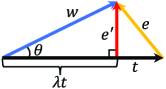
Figure 1: Scalar Constant $\lambda$ of a Ternary Vector

This increases the necessary memory size (footprint), but is effective to improve accuracy. Moreover, if $\bm{t}$ includes both positive and negative elements, we could improve the accuracy more by memorizing one more scalar: We let $\bm{t}=\bm{t}_{p}-\bm{t}_{n}$ with $\bm{t}_{p}\geq 0$ and $\bm{t}_{n}\leq 0$ and $\bm{w}=\bm{w}_{p}-\bm{w}_{n}$ with $\bm{w}_{p}\geq 0$ and $\bm{w}_{n}\leq 0$: for a vector $\bm{v}$, $\bm{v}\geq 0$ ($\bm{v}\leq 0$) means that all the elements of $\bm{v}$ is non-negative (non-positive). We should note that $\bm{t}_{p}\cdot\bm{t}_{n}=\bm{t}_{p}\cdot\bm{w}_{n}=\bm{w}_{p}\cdot\bm{t}_{n}=\bm{w}_{p}\cdot\bm{w}_{n}=0$, $\bm{t}_{p}\cdot\bm{w}_{p}\geq 0$ and $\bm{t}_{n}\cdot\bm{w}_{n}\geq 0$ holds. Therefore, we have:

$$\left\|\bm{w}-\frac{\bm{w}\cdot\bm{t}}{\bm{t}\cdot\bm{t}}\bm{t}\right\|_{2}^{2} =\bm{w}\cdot\bm{w}-\frac{(\bm{w}\cdot\bm{t})^{2}}{\bm{t}\cdot\bm{t}}$$

$$=\bm{w}_{p}\cdot\bm{w}_{p}+\bm{w}_{n}\cdot\bm{w}_{n}-\frac{(\bm{w}_{p}\cdot\bm{t}_{p}+\bm{w}_{n}\cdot\bm{t}_{n})^{2}}{\bm{t}_{p}\cdot\bm{t}_{p}+\bm{t}_{n}\cdot\bm{t}_{n}}$$

$$\geq\bm{w}_{p}\cdot\bm{w}_{p}-\frac{(\bm{w}_{p}\cdot\bm{t}_{p})^{2}}{\bm{t}_{p}\cdot\bm{t}_{p}}+\bm{w}_{n}\cdot\bm{w}_{n}-\frac{(\bm{w}_{n}\cdot\bm{t}_{n})^{2}}{\bm{t}_{n}\cdot\bm{t}_{n}}$$

$$=\left\|\bm{w}_{p}-\frac{\bm{w}_{p}\cdot\bm{t}_{p}}{\bm{t}_{p}\cdot\bm{t}_{p}}\bm{t}_{p}\right\|_{2}^{2}+\left\|\bm{w}_{n}-\frac{\bm{w}_{n}\cdot\bm{t}_{n}}{\bm{t}_{n}\cdot\bm{t}_{n}}\bm{t}_{n}\right\|_{2}^{2}.$$

Thus, if we let $\lambda_{p}=\frac{\bm{w}_{p}\cdot\bm{t}_{p}}{\|\bm{t}_{p}\|}$ and $\lambda_{n}=\frac{\bm{w}_{n}\cdot\bm{t}_{n}}{\|\bm{t}_{n}\|}$ memorized in addition to $\bm{t}$, we can not only save memory size but also suppress loss of accuracy.

3 Simulations

In this part, we first show the performance of our TNT method on transforming target vectors to ternary vectors. Then, we show the upper limit of similarity of ternary and binary when utilizing different distributions to initialize target vectors. Finally, we demonstrate an example using TNT to convert weights of DNN models to ternary. All experiments are run on a PC with Intel(R) Core(TM) i7-8700 CPU at 3.2GHz using 32GB of RAM and a NVIDIA GeForce GTX 1080 graphics card, running Windows 10 system.

3.1 Converting Performance

In order to investigate the accuracy performance of our ternarization method, we prepare two target vectors of dimension 1,000,000: one has elements determined independently following a uniform distribution; The other follows a normal distribution instead. Figure 2 (a) shows the cosine similarity scores observed when we change the number $M$ of non-zero elements of $\bm{t}$. The highest score for the target vector that has followed a uniform distribution is $0.94$ when $667,033$ elements of $\bm{t}$ are non-zero, while the highest score is $0.90$ for a normal distribution when $540,349$ elements of $\bm{t}$ are non-zero. The curves of the cosine similarity score are unimodal, and if this always holds true, finding maximum cosine similarity scores can be easier.

Moreover, we found a fact that the cosine similarity is not easily affected by the dimension of a ternary or binary vector. We calculated 10000 times of the maximum cosine similarity with the dimension of target vectors increases by one at each time. Figure 2 (b) and (c) show the simulation results: 1) regardless of the target vector under normal distribution or uniform distribution, ternary vectors reserve a higher similarity. 2) the cosine similarity of ternary and binary vectors converge to a stable value with the increasing of vector dimension, and the ternary vector has a smaller variance comparing with the binary vector.

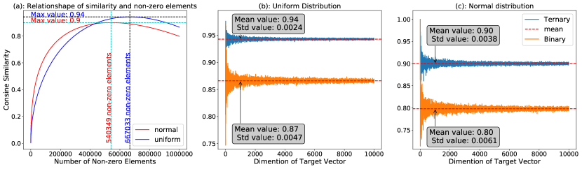
Figure 2: Simulation Result of Cosine Similarity by TNT method

3.2 Performance on Neural Networks

We perform our experiments on LeNet-5[4], VGG-7[4], and VGG16[8] using MNIST, CIFAR-10, and ImageNet datasets respectively to first train a full precision network model, and then replace the floating point parameters by the ternary parameters obtained by the proposed TNT. A precise comparison between floating point model and ternary model is conducted.

The experiment results are shown in Table 1. It shows that, without network retraining, inferences with ternary parameters only lose $0.21\%$ and $0.14\%$ of accuracies using LeNet-5 and VGG-7 respectively on MNIST dataset. And it loses $2.22\%$ of accuracy for VGG-7 on CIFAR-10 dataset. For VGG-16 network on ImageNet dataset, the Top-1 and Top-5 accuracy dropped $8\%$ and $5.34\%$, respectively. Moreover, the memory size of LeNet-5 and VGG-7 are reduced $16$ times since each ternary weight only requires $2$ bits of memory. On the other hand, because of converting the first and last layer of VGG-16 to ternary without fine-tuning has a significant affection on the accuracy, which is the same phenomenon mentioned in [7], we do not convert the first and the last layer in VGG-16, and the parameter size reduces $11.1$ times.

Table 1: TNT Performance on Neural Networks

Network	Base Line	TNT Converted	Parameters	Converting Times
LeNet-5 (MNIST)	99.18%	98.97%	1,663,370	7.803s
VGG-7 (CIFAR-10)	91.31%	89.09%	7,734,410	88.288s
VGG-16 (ImageNet)	64.26%, 85.59%	56.26%, 80.25%	12,976,266	115.863s

4 Conclusions

In this paper, we proposed a target non-retraining ternary (TNT) method to convert a full precision parameters model to a ternary parameters model accurately and quickly without retraining of the network. In our approach, firstly, we succeeded in reducing the size of the searching range from $3^{N}$ to $N$ by evaluating the cosine similarity between a target vector and a ternary vector. Secondly, scaling-tuning factors are proposed coupling with the cosine similarity to further enable the TNT to find the best ternary vector. Due to the smart tricks, TNT’s computational complexity is only $O(N\log N)$. Thirdly, we showed that the distributions of parameters have an obvious affection on the weight converting result. This implies that the initial distributions for parameters are important. Moreover, we applied the TNT to several models. As a result, we verified that quantization by our TNT method caused a small loss of accuracy.

References

- Courbariaux et al. [2015] Matthieu Courbariaux, Yoshua Bengio, and Jean-Pierre David. Binaryconnect: Training deep neural networks with binary weights during propagations. In Advances in neural information processing systems, pages 3123–3131, 2015.
- Rastegari et al. [2016] Mohammad Rastegari, Vicente Ordonez, Joseph Redmon, and Ali Farhadi. Xnor-net: Imagenet classification using binary convolutional neural networks. In European Conference on Computer Vision, pages 525–542. Springer, 2016.
- Hubara et al. [2016] Itay Hubara, Matthieu Courbariaux, Daniel Soudry, Ran El-Yaniv, and Yoshua Bengio. Binarized neural networks. In Advances in neural information processing systems, pages 4107–4115, 2016.
- Li et al. [2016] Fengfu Li, Bo Zhang, and Bin Liu. Ternary weight networks. arXiv preprint arXiv:1605.04711, 2016.
- Deng et al. [2018] Lei Deng, Peng Jiao, Jing Pei, Zhenzhi Wu, and Guoqi Li. Gxnor-net: Training deep neural networks with ternary weights and activations without full-precision memory under a unified discretization framework. Neural Networks, 100:49–58, 2018.
- Alemdar et al. [2017] Hande Alemdar, Vincent Leroy, Adrien Prost-Boucle, and Frédéric Pétrot. Ternary neural networks for resource-efficient ai applications. In 2017 International Joint Conference on Neural Networks (IJCNN), pages 2547–2554. IEEE, 2017.
- Mellempudi et al. [2017] Naveen Mellempudi, Abhisek Kundu, Dheevatsa Mudigere, Dipankar Das, Bharat Kaul, and Pradeep Dubey. Ternary neural networks with fine-grained quantization. arXiv preprint arXiv:1705.01462, 2017.
- Simonyan and Zisserman [2014] Karen Simonyan and Andrew Zisserman. Very deep convolutional networks for large-scale image recognition. arXiv preprint arXiv:1409.1556, 2014.