Scalable Resilience Against Node Failures for Communication-Hiding Preconditioned Conjugate Gradient and Conjugate Residual Methods

Abstract

The observed and expected continued growth in the number of nodes in large-scale parallel computers gives rise to two major challenges: global communication operations are becoming major bottlenecks due to their limited scalability, and the likelihood of node failures is increasing. We study an approach for addressing these challenges in the context of solving large sparse linear systems. In particular, we focus on the pipelined preconditioned conjugate gradient (PPCG) method, which has been shown to successfully deal with the first of these challenges. In this paper, we address the second challenge. We present extensions to the PPCG solver and two of its variants which make them resilient against the failure of a compute node while fully preserving their communication-hiding properties and thus their scalability. The basic idea is to efficiently communicate a few redundant copies of local vector elements to neighboring nodes with very little overhead. In case a node fails, these redundant copies are gathered at a replacement node, which can then accurately reconstruct the lost parts of the solver’s state. After that, the parallel solver can continue as in the failure-free scenario. Experimental evaluations of our approach illustrate on average very low runtime overheads compared to the standard non-resilient algorithms. This shows that scalable algorithmic resilience can be achieved at low extra cost.

1 Introduction

The conjugate gradient (CG) and conjugate residual (CR) algorithms as well as their preconditioned variants (PCG and PCR) are widely used iterative Krylov subspace methods for solving linear systems $\bm{A}\bm{x}=\bm{b}$ [35, 48]. In many scientific applications, these linear systems are obtained from discretizing partial differential equations that model the simulated problems. The resulting system matrix $\bm{A}$ then typically is sparse and may contain only a very small number of non-zero elements per row. Both solvers are frequently run in parallel and are expected to be viable choices for upcoming large-scale parallel computers with hundreds of thousand or even millions of compute nodes.

However, two major challenges have to be overcome in order to optimize the PCG and PCR methods for such large parallel computers. Firstly, communication between a substantial fraction or even all of the compute nodes, i.e., global communication, becomes increasingly expensive with a growing total number $N$ of nodes. This is particularly true for computing the dot products in each iteration of PCG and PCR, which involves costly global synchronization. The cost of a global reduction operation is $\mathcal{O}(\log N)$ and, thus, steadily grows with an increasing number of nodes [32, 36]. Secondly, the reliability of computer clusters is predicted to deteriorate at scale. A compute node of a cluster may fail for many different reasons, e.g., some hardware component malfunctions, the shared memory gets corrupted, or it loses its connection to the interconnection network. If we assume a—rather optimistic—mean time between failures (MTBF) of a century for an individual node, a cluster with ${10}^{5}$ nodes, on average, will encounter a node failure every nine hours. Even worse, a system with ${10}^{6}$ nodes will encounter a node failure every 53 minutes on average [34]. Therefore, we have to expect possibly several node failures during the execution of a long-running scientific application.

To tackle the first challenge, solvers that try to either reduce global communication or overlap global communication with both computation and local communication have been suggested. These two classes of solvers are commonly referred to as communication-avoiding and communication-hiding solvers, respectively. Early communication-avoiding CG methods comprise variants of the original algorithm with only a single global synchronization point [6, 24, 23, 28, 43, 47] as well as a CG variation with two three-term recurrences and only one reduction operation [48]. For reducing global communication even further, $s$-step methods have been introduced [11, 14, 37] and recently applied in large-scale simulations [38, 40]. These methods accomplish to reduce the number of global synchronizations by $\mathcal{O}(s)$ through computing the CG iterations in blocks of $s$. However, $s$-step methods tend to become numerically unstable with increasing $s$. Another approach for reducing global communication has been to enlarge the Krylov subspace [33].

Besides the overall reduction of global synchronization points, it has early been suggested to overlap the dot products in the CG method with computation [25, 26]. This principle has been enhanced by Ghysels et al. [31, 32] with the introduction of pipelined solvers, first for the generalized minimal residual (GMRES) method and later for PCG. The pipelined PCG (PPCG) algorithm performs only a single non-blocking reduction per iteration and overlaps this global communication with the application of the preconditioner as well as the computation of the sparse matrix-vector product (SpMV), which often requires solely local communication [32]. Based on PPCG, Ghysels and Vanroose derive the closely related pipelined PCR (PPCR) algorithm [32]. Both PPCG and PPCR are readily available in the widely used parallel numerical library PETSc [4, 5]. Moreover, several studies investigate the numerical properties and performance of the PPCG method [12, 19, 20, 15, 17, 16]. Others propose modified or alternative pipelined PCG methods [21, 18, 29, 49], one of them being the two-iteration pipelined PCG (2PPCG) algorithm by Eller and Gropp [29], which is based on a three-term recurrence variant of PCG.

To overcome the second challenge described above, different general-purpose and algorithm-specific fault-tolerance approaches have been discussed in the literature. Nowadays, the most commonly applied measures against node failures are various checkpointing and rollback-recovery techniques, which frequently save the full state of an executed application and restore the latest one in case of a node failure [34, 52]. To avoid the usually considerable overhead of continuously saving the state of an entire application, Chen [13] and Pachajoa et al. [45, 46] exploit the inherent redundancy of the SpMV in PCG. A well-defined strategy ensures enough redundant copies of the search direction vectors in order to fully recover the whole state of PCG after possibly multiple simultaneous node failures. An alternative approach by Langou et al. [39] and Agullo et al. [2, 3] approximates the lost part of the latest solution vector, which is then used as the initial guess for the restarted solver. Bosilca et al. [8, 9, 34] suggest an algorithm for integrating algorithm-specific with general-purpose fault-tolerance techniques. While Pachajoa and Gansterer [44] evaluate the inherent resilience properties of CG after a node failure, others discuss the related but independent problem of soft errors in CG [1, 10, 27, 30, 50, 51].

In this work, we target the problem of solving large sparse symmetric and positive-definite (SPD) linear systems $\bm{A}\bm{x}=\bm{b}$ on parallel computers that both are susceptible to node failures and have high cost of global communication compared to computation and local communication. For this purpose, we introduce an innovative combination of communication-hiding solvers and algorithm-specific resilience against node failures. We focus on the broadly discussed PPCG solver [12, 19, 20, 15, 17, 16, 32] but also consider the PPCR [32] and 2PPCG [29] algorithms. For coping with node failures, we propose novel recovery methods for the PPCG, PPCR, and 2PPCG solvers, which are partly related to the techniques for the PCG method suggested by Chen [13] and Pachajoa et al. [45, 46]. Those techniques are likely to be more scalable—i.e., better suited for large-scale computer clusters—than general-purpose fault-tolerance techniques. In numerical experiments, we demonstrate low runtime overheads of our resilient PPCG algorithm.

Algorithm 1 Preconditioned conjugate gradient (PCG) method [48, Alg. 9.1]

1:$\bm{r}^{(0)}\leftarrow\bm{b}-\bm{A}\bm{x}^{(0)}$, $\bm{u}^{(0)}\leftarrow\bm{M}^{-1}\bm{r}^{(0)}$, $\bm{p}^{(0)}\leftarrow\bm{u}^{(0)}$

2:$\gamma^{(0)}\leftarrow(\bm{r}^{(0)},\bm{u}^{(0)})$

3:for $i\leftarrow 0,1,\dots,\text{until convergence}$ do

4:     $\bm{s}^{(i)}\leftarrow\bm{A}\bm{p}^{(i)}$

5:     $\delta^{(i)}\leftarrow(\bm{s}^{(i)},\bm{p}^{(i)})$

6:     $\alpha^{(i)}\leftarrow\gamma^{(i)}/\delta^{(i)}$

7:     $\bm{x}^{(i+1)}\leftarrow\bm{x}^{(i)}+\alpha^{(i)}\bm{p}^{(i)}$

8:     $\bm{r}^{(i+1)}\leftarrow\bm{r}^{(i)}-\alpha^{(i)}\bm{s}^{(i)}$

9:     $\bm{u}^{(i+1)}\leftarrow\bm{M}^{-1}\bm{r}^{(i+1)}$

10:     $\gamma^{(i+1)}\leftarrow(\bm{r}^{(i+1)},\bm{u}^{(i+1)})$

11:     $\beta^{(i)}\leftarrow\gamma^{(i+1)}/\gamma^{(i)}$

12:     $\bm{p}^{(i+1)}\leftarrow\bm{u}^{(i+1)}+\beta^{(i)}\bm{p}^{(i)}$

13:end for

1.1 Terminology and assumptions

As a consequence of a node failure, the affected node becomes unavailable, and a node that replaces it in the recovery process is called a replacement node. The replacement node is either a spare node or one of the surviving nodes. In this paper, we assume that the parallel runtime environment provides functionality comparable to state-of-the-art implementations of the industry-standard Message Passing Interface (MPI) [41]. Moreover, we assume that the runtime environment provides some basic fault-tolerance features. A prototypical example is the User Level Failure Mitigation (ULFM) framework [7, 42], an extension of the MPI standard. It supports basic functionality which our approach is based on, including the detection of node failures, preventing indefinitely blocking synchronizations or communications, notifying the surviving nodes which nodes have failed, and a mechanism for providing replacement nodes.

Like in widely used libraries such as PETSc [4, 5], we use a block-row data distribution of all sparse matrices and vectors across the $N$ nodes of the parallel system. In particular, for an $n\times n$ linear system, every node owns blocks of $n/N$ contiguous rows (if $n=cN$ with $c\in\mathbb{N}$, otherwise some nodes own $\lfloor n/N\rfloor$ and others $\lceil n/N\rceil$ rows) of all matrices and vectors involved. On a single node, the data block stored in its shared memory is evenly distributed among the processors of the node. Since each node owns rows of all matrices and vectors involved, a node failure leads to the loss of a part of every matrix and vector. With the state of an iterative solver we mean the—not necessarily minimal—set of data that completely determines the future behavior of this iterative solver.

Given a vector $\bm{v}^{(i)}$, where $i$ denotes the iteration number of the linear solver, $\bm{v}_{j}^{(i)}$ refers to the subset of elements of the vector at iteration $i$ owned by node $j$. For a matrix $\bm{B}$, the block of rows of $\bm{B}$ owned by node $j$ is denoted by $\bm{B}_{j\star}$. On the other hand, $\bm{B}_{\star k}$ is the block of columns of $\bm{B}$ corresponding to the indices of the rows owned by node $k$. Consequently, $\bm{B}_{jk}$ is the submatrix consisting of the rows owned by node $j$ and the columns corresponding to the indices of the rows owned by node $k$. $\bar{k}$ stands for all indices except for those of node $k$. $[\bm{v},\bm{w}]$ denotes the concatenation of vectors $\bm{v}$ and $\bm{w}$ to a matrix. The failed node as well as the replacement node are referred to as node $\rho$.

Algorithm 2 Pipelined preconditioned conjugate gradient (PPCG) method [32, Alg. 4]

1:$\bm{r}^{(0)}\leftarrow\bm{b}-\bm{A}\bm{x}^{(0)}$, $\bm{u}^{(0)}\leftarrow\bm{M}^{-1}\bm{r}^{(0)}$, $\bm{w}^{(0)}\leftarrow\bm{A}\bm{u}^{(0)}$

2:for $i\leftarrow 0,1,\dots,\text{until convergence}$ do

3:     $\gamma^{(i)}\leftarrow(\bm{r}^{(i)},\bm{u}^{(i)})$, $\delta^{(i)}\leftarrow(\bm{w}^{(i)},\bm{u}^{(i)})$

4:     $\bm{m}^{(i)}\leftarrow\bm{M}^{-1}\bm{w}^{(i)}$

5:     $\bm{n}^{(i)}\leftarrow\bm{A}\bm{m}^{(i)}$

6:     if $i=0$ then

7:         $\alpha^{(i)}\leftarrow\gamma^{(i)}/\delta^{(i)}$, $\beta^{(i)}\leftarrow 0$

8:     else

9:         $\beta^{(i)}\leftarrow\gamma^{(i)}/\gamma^{(i-1)}$

10:         $\alpha^{(i)}\leftarrow\gamma^{(i)}/(\delta^{(i)}-\beta^{(i)}\gamma^{(i)}/\alpha^{(i-1)})$

11:     end if

12:     $\bm{z}^{(i)}\leftarrow\bm{n}^{(i)}+\beta^{(i)}\bm{z}^{(i-1)}$

13:     $\bm{q}^{(i)}\leftarrow\bm{m}^{(i)}+\beta^{(i)}\bm{q}^{(i-1)}$

14:     $\bm{s}^{(i)}\leftarrow\bm{w}^{(i)}+\beta^{(i)}\bm{s}^{(i-1)}$

15:     $\bm{p}^{(i)}\leftarrow\bm{u}^{(i)}+\beta^{(i)}\bm{p}^{(i-1)}$

16:     $\bm{x}^{(i+1)}\leftarrow\bm{x}^{(i)}+\alpha^{(i)}\bm{p}^{(i)}$

17:     $\bm{r}^{(i+1)}\leftarrow\bm{r}^{(i)}-\alpha^{(i)}\bm{s}^{(i)}$

18:     $\bm{u}^{(i+1)}\leftarrow\bm{u}^{(i)}-\alpha^{(i)}\bm{q}^{(i)}$

19:     $\bm{w}^{(i+1)}\leftarrow\bm{w}^{(i)}-\alpha^{(i)}\bm{z}^{(i)}$

20:end for

1.2 Main contributions

Although communication-hiding (along with communication-avoiding) iterative solvers and algorithm-specific resilience techniques against node failures are both motivated by the specific properties of future large-scale parallel computers, there has been, to the best of our knowledge, no attempt so far to combine the advantages of those two approaches. In this paper, we propose novel strategies for recovery after node failures occurred during the execution of the communication-hiding PPCG [12, 19, 20, 15, 17, 16, 32] as well as PPCR [32] and 2PPCG [29] solvers. To this end, we build upon recent work by Chen [13] and Pachajoa et al. [45, 46] regarding resilience against node failures for the classical PCG solver. We eventually show the low runtime overhead of our new fault-tolerant PPCG solver in numerical experiments.

The remainder of the paper is structured as follows. First, in LABEL:Sectionsecsolvers, we discuss in more detail the considered communication-hiding solvers including their most important properties. Next, in LABEL:Sectionsecredundancy, we review how to ensure enough data redundancy for coping with node failures in the PCG method and illustrate the relevance for the PPCG, PPCR, and 2PPCG algorithms. Then, in LABEL:Sectionsecrecovery, we derive and describe our novel strategies for recovering the full state of PPCG and the other solvers after node failures occurred. After that, in LABEL:Sectionsecexperiments, we outline our experiments and present the results. Finally, in LABEL:Sectionsecconclusions, we summarize our conclusions.

2 Communication-hiding iterative solvers

Algorithm 3 Pipelined preconditioned conjugate residual (PPCR) method [32, Alg. 5]

1:$\bm{r}^{(0)}\leftarrow\bm{b}-\bm{A}\bm{x}^{(0)}$, $\bm{u}^{(0)}\leftarrow\bm{M}^{-1}\bm{r}^{(0)}$, $\bm{w}^{(0)}\leftarrow\bm{A}\bm{u}^{(0)}$

2:for $i\leftarrow 0,1,\dots,\text{until convergence}$ do

3:     $\bm{m}^{(i)}\leftarrow\bm{M}^{-1}\bm{w}^{(i)}$

4:     $\gamma^{(i)}\leftarrow(\bm{w}^{(i)},\bm{u}^{(i)})$, $\delta^{(i)}\leftarrow(\bm{m}^{(i)},\bm{w}^{(i)})$

5:     $\bm{n}^{(i)}\leftarrow\bm{A}\bm{m}^{(i)}$

6:     if $i=0$ then

7:         $\alpha^{(i)}\leftarrow\gamma^{(i)}/\delta^{(i)}$, $\beta^{(i)}\leftarrow 0$

8:     else

9:         $\beta^{(i)}\leftarrow\gamma^{(i)}/\gamma^{(i-1)}$

10:         $\alpha^{(i)}\leftarrow\gamma^{(i)}/(\delta^{(i)}-\beta^{(i)}\gamma^{(i)}/\alpha^{(i-1)})$

11:     end if

12:     $\bm{z}^{(i)}\leftarrow\bm{n}^{(i)}+\beta^{(i)}\bm{z}^{(i-1)}$

13:     $\bm{q}^{(i)}\leftarrow\bm{m}^{(i)}+\beta^{(i)}\bm{q}^{(i-1)}$

14:     $\bm{p}^{(i)}\leftarrow\bm{u}^{(i)}+\beta^{(i)}\bm{p}^{(i-1)}$

15:     $\bm{x}^{(i+1)}\leftarrow\bm{x}^{(i)}+\alpha^{(i)}\bm{p}^{(i)}$

16:     $\bm{u}^{(i+1)}\leftarrow\bm{u}^{(i)}-\alpha^{(i)}\bm{q}^{(i)}$

17:     $\bm{w}^{(i+1)}\leftarrow\bm{w}^{(i)}-\alpha^{(i)}\bm{z}^{(i)}$

18:end for

In this section, we review the basic ideas and main properties of the communication-hiding iterative linear solvers we later consider in the context of fault tolerance. We first study the PPCG method [32] in LABEL:Sectionsecsolvers:ppcg, including its foundations in the original PCG algorithm [35, 48]. Subsequently, in LABEL:Sectionsecsolvers:other, we briefly highlight the modifications that lead to the PPCR algorithm [32] and discuss an alternative to the PPCG solver, the 2PPCG method [29].

2.1 Pipelined PCG

The communication-hiding PPCG solver [32] is a reformulation of the classical PCG method [35, 48]. Let $\bm{A}\in\mathbb{R}^{n\times n}$ be an SPD matrix and $\bm{M}^{-1}\in\mathbb{R}^{n\times n}$ be an appropriate SPD preconditioner for $\bm{A}$, i.e., $\kappa(\bm{M}^{-1}\bm{A})<\kappa(\bm{A})$, where $\kappa(\bm{B})$ denotes the condition number of a matrix $\bm{B}$. Furthermore, let $\bm{b}\in\mathbb{R}^{n}$ and $\bm{x}\in\mathbb{R}^{n}$ be the right-hand-side and solution vectors, respectively. For iteratively solving a given sparse linear system $\bm{A}\bm{x}=\bm{b}$, the PCG method, which is listed in LABEL:Algorithmalgpcg, actually solves the left-preconditioned linear system $\bm{M}^{-1}\bm{A}\bm{x}=\bm{M}^{-1}\bm{b}$ for accelerated convergence. After the solver has converged, the iterate $\bm{x}^{(i)}$ is reasonably close to the solution vector $\bm{x}$. The search direction vectors $\bm{p}^{(i)}$ are chosen to be mutually $\bm{A}$-orthogonal, i.e., $(\bm{A}\bm{p}^{(i)},\bm{p}^{(j)})=0$ for all $i\neq j$. The residual vector $\bm{r}^{(i)}$ is defined by the relation $\bm{r}^{(i)}=\bm{b}-\bm{A}\bm{x}^{(i)}$. Additionally, the PCG solver keeps the preconditioned residual vector $\bm{u}^{(i)}\coloneqq\bm{M}^{-1}\bm{r}^{(i)}$ and the vector $\bm{s}^{(i)}\coloneqq\bm{A}\bm{p}^{(i)}$. For computing the dot products, there are two global synchronization points in each iteration of PCG (lines 5 and 10 of LABEL:Algorithmalgpcg). Since the results of those dot products are needed immediately afterwards, both global communication operations are blocking.

For being able to reorder the PCG operations such that we have only one global synchronization point and the possibility to overlap global communication with computation and local communication, the PPCG method, which is shown in LABEL:Algorithmalgppcg, has to keep the five additional vectors $\bm{w}^{(i)}\coloneqq\bm{A}\bm{u}^{(i)}$, $\bm{m}^{(i)}\coloneqq\bm{M}^{-1}\bm{w}^{(i)}$, $\bm{n}^{(i)}\coloneqq\bm{A}\bm{m}^{(i)}$, $\bm{q}^{(i)}\coloneqq\bm{M}^{-1}\bm{s}^{(i)}$, and $\bm{z}^{(i)}\coloneqq\bm{A}\bm{q}^{(i)}$. By left-multiplying $\bm{A}$ and $\bm{M}^{-1}$ to relations of the original PCG algorithm, Ghysels and Vanroose [32] derive new recurrence relations that allow them to reorder and merge the two dot product computations to just one global reduction operation (LABEL:linealgppcg:gammadelta of LABEL:Algorithmalgppcg). Furthermore, since the results of the dot products are not needed before lines 7 and 9 of LABEL:Algorithmalgppcg, the global reductions can be computed as non-blocking operations and, therefore, can be overlapped with the application of the preconditioner as well as the SpMV computation in lines 4 and 5 of LABEL:Algorithmalgppcg. These two operations typically require only local communication. However, the PPCG method has to compute eight (lines 12 to 19 of LABEL:Algorithmalgppcg) instead of just three vector updates as in the PCG algorithm. Although both solvers are mathematically equivalent, we may see different numerical error propagation in finite precision [32].

2.2 Other solvers

Algorithm 4 Two-iteration pipelined preconditioned conjugate gradient (2PPCG) method [29]

1:$\bm{r}^{(0)}\leftarrow\bm{b}-\bm{A}\bm{x}^{(0)}$, $\bm{u}^{(0)}\leftarrow\bm{M}^{-1}\bm{r}^{(0)}$, $\bm{w}^{(0)}\leftarrow\bm{A}\bm{u}^{(0)}$

2:$\gamma^{(0)}\leftarrow(\bm{u}^{(0)},\bm{r}^{(0)})$, $\delta^{(0)}\leftarrow(\bm{u}^{(0)},\bm{w}^{(0)})$

3:$\bm{m}^{(0)}\leftarrow\bm{M}^{-1}\bm{w}^{(0)}$, $\bm{n}^{(0)}\leftarrow\bm{A}\bm{m}^{(0)}$

4:$\bm{c}^{(0)}\leftarrow\bm{M}^{-1}\bm{n}^{(0)}$, $\bm{d}^{(0)}\leftarrow\bm{A}\bm{c}^{(0)}$

5:for $i\leftarrow 0,2,\dots,\text{until convergence}$ do

6:     if $i=0$ then

7:         $\zeta^{(i+1)}\leftarrow 1$, $\eta^{(i+1)}\leftarrow\gamma^{(i)}/\delta^{(i)}$, $\theta^{(i+1)}\leftarrow 0$

8:     else

9:         $\eta^{(i)}\leftarrow\gamma^{(i-1)}/\delta^{(i-1)}$

10:         $\zeta^{(i)}\leftarrow 1/(1-\gamma^{(i-1)}\eta^{(i)}/(\gamma^{(i-2)}\zeta^{(i-1)}\eta^{(i-1)}))$

11:         $\kappa_{1}\leftarrow\zeta^{(i)}$, $\kappa_{2}\leftarrow-\zeta^{(i)}\eta^{(i)}$, $\kappa_{3}\leftarrow 1-\zeta^{(i)}$

12:         $\gamma^{(i)}\leftarrow\kappa_{1}\kappa_{1}\lambda_{1}-2\kappa_{1}\kappa_{2}\lambda_{7}+2\kappa_{1}\kappa_{3}\lambda_{6}$

13:$\hskip 15.00002pt\hskip 15.00002pt\hphantom{\gamma^{(i)}\leftarrow}\mathllap{+}\;\kappa_{2}\kappa_{2}\lambda_{2}-2\kappa_{2}\kappa_{3}\lambda_{3}+\kappa_{3}\kappa_{3}\lambda_{8}$

14:         $\delta^{(i)}\leftarrow\kappa_{1}\kappa_{1}\lambda_{7}-2\kappa_{1}\kappa_{2}\lambda_{2}+2\kappa_{1}\kappa_{3}\lambda_{3}$

15:$\hskip 15.00002pt\hskip 15.00002pt\hphantom{\delta^{(i)}\leftarrow}\mathllap{+}\;\kappa_{2}\kappa_{2}\lambda_{4}-2\kappa_{2}\kappa_{3}\lambda_{5}+\kappa_{3}\kappa_{3}\lambda_{8}$

16:         $\eta^{(i+1)}\leftarrow\gamma^{(i)}/\delta^{(i)}$

17:         $\zeta^{(i+1)}\leftarrow 1/(1-\gamma^{(i)}\eta^{(i+1)}/(\gamma^{(i-1)}\zeta^{(i)}\eta^{(i)}))$

18:         $\theta^{(i)}\leftarrow\kappa_{3}$, $\theta^{(i+1)}\leftarrow 1-\zeta^{(i+1)}$

19:         $\bm{x}^{(i)}\leftarrow\zeta^{(i)}(\bm{x}^{(i-1)}+\eta^{(i)}\bm{u}^{(i-1)})+\theta^{(i)}\bm{x}^{(i-2)}$

20:         $\bm{r}^{(i)}\leftarrow\zeta^{(i)}(\bm{r}^{(i-1)}-\eta^{(i)}\bm{w}^{(i-1)})+\theta^{(i)}\bm{r}^{(i-2)}$

21:         $\bm{u}^{(i)}\leftarrow\zeta^{(i)}(\bm{u}^{(i-1)}-\eta^{(i)}\bm{m}^{(i-1)})+\theta^{(i)}\bm{u}^{(i-2)}$

22:         $\bm{w}^{(i)}\leftarrow\zeta^{(i)}(\bm{w}^{(i-1)}-\eta^{(i)}\bm{n}^{(i-1)})+\theta^{(i)}\bm{w}^{(i-2)}$

23:         $\bm{m}^{(i)}\leftarrow\zeta^{(i)}(\bm{m}^{(i-1)}-\eta^{(i)}\bm{c}^{(i-1)})+\theta^{(i)}\bm{m}^{(i-2)}$

24:         $\bm{n}^{(i)}\leftarrow\zeta^{(i)}(\bm{n}^{(i-1)}-\eta^{(i)}\bm{d}^{(i-1)})+\theta^{(i)}\bm{n}^{(i-2)}$

25:         $\bm{c}^{(i)}\leftarrow\zeta^{(i)}(\bm{c}^{(i-1)}-\eta^{(i)}\bm{g}^{(i-1)})+\theta^{(i)}\bm{c}^{(i-2)}$

26:         $\bm{d}^{(i)}\leftarrow\zeta^{(i)}(\bm{d}^{(i-1)}-\eta^{(i)}\bm{h}^{(i-1)})+\theta^{(i)}\bm{d}^{(i-2)}$

27:     end if

28:     $\bm{x}^{(i+1)}\leftarrow\zeta^{(i+1)}(\bm{x}^{(i)}+\eta^{(i+1)}\bm{u}^{(i)})+\theta^{(i+1)}\bm{x}^{(i-1)}$

29:     $\bm{r}^{(i+1)}\leftarrow\zeta^{(i+1)}(\bm{r}^{(i)}-\eta^{(i+1)}\bm{w}^{(i)})+\theta^{(i+1)}\bm{r}^{(i-1)}$

30:     $\bm{u}^{(i+1)}\leftarrow\zeta^{(i+1)}(\bm{u}^{(i)}-\eta^{(i+1)}\bm{m}^{(i)})+\theta^{(i+1)}\bm{u}^{(i-1)}$

31:     $\bm{w}^{(i+1)}\leftarrow\zeta^{(i+1)}(\bm{w}^{(i)}-\eta^{(i+1)}\bm{n}^{(i)})+\theta^{(i+1)}\bm{w}^{(i-1)}$

32:     $\bm{m}^{(i+1)}\leftarrow\zeta^{(i+1)}(\bm{m}^{(i)}-\eta^{(i+1)}\bm{c}^{(i)})+\theta^{(i+1)}\bm{m}^{(i-1)}$

33:     $\bm{n}^{(i+1)}\leftarrow\zeta^{(i+1)}(\bm{n}^{(i)}-\eta^{(i+1)}\bm{d}^{(i)})+\theta^{(i+1)}\bm{n}^{(i-1)}$

34:     $\lambda_{1}\leftarrow(\bm{u}^{(i+1)},\bm{w}^{(i+1)})$, $\lambda_{2}\leftarrow(\bm{u}^{(i+1)},\bm{w}^{(i)})$

35:     $\lambda_{3}\leftarrow(\bm{m}^{(i+1)},\bm{n}^{(i+1)})$, $\lambda_{4}\leftarrow(\bm{m}^{(i+1)},\bm{w}^{(i)})$

36:     $\lambda_{5}\leftarrow(\bm{u}^{(i)},\bm{w}^{(i)})$, $\lambda_{6}\leftarrow(\bm{u}^{(i+1)},\bm{r}^{(i)})$

37:     $\lambda_{7}\leftarrow(\bm{u}^{(i)},\bm{r}^{(i)})$, $\lambda_{8}\leftarrow(\bm{u}^{(i+1)},\bm{u}^{(i+1)})$

38:     $\gamma^{(i+1)}\leftarrow(\bm{u}^{(i+1)},\bm{r}^{(i+1)})$, $\delta^{(i+1)}\leftarrow\lambda_{1}$

39:     $\bm{c}^{(i+1)}\leftarrow\bm{M}^{-1}\bm{n}^{(i+1)}$, $\bm{d}^{(i+1)}\leftarrow\bm{A}\bm{c}^{(i+1)}$

40:     $\bm{g}^{(i+1)}\leftarrow\bm{M}^{-1}\bm{d}^{(i+1)}$, $\bm{h}^{(i+1)}\leftarrow\bm{A}\bm{g}^{(i+1)}$

41:end for

When the $\bm{M}$ inner product that is used for the dot products in PPCG is replaced by the $\bm{A}$ inner product ($\bm{M}^{-1}\bm{A}$ is also self-adjoint with respect to this inner product), we obtain the PPCR method, which is listed in LABEL:Algorithmalgppcr, as a variation of the PPCG solver [32]. Since the preconditioner has then to be applied before the dot products, the merged global reduction operation (LABEL:linealgppcr:gammadelta of LABEL:Algorithmalgppcr) can only be overlapped with the SpMV computation (LABEL:linealgppcr:n of LABEL:Algorithmalgppcr). Moreover, there is no dependence on $\bm{r}^{(i)}$ and $\bm{s}^{(i)}$ anymore and, hence, those vectors do not need to be updated in every iteration. In this case, the convergence criterion can be based on the preconditioned residual $\bm{u}^{(i)}$ instead of the residual $\bm{r}^{(i)}$.

Eller and Gropp [29] suggest an alternative pipelined PCG algorithm based on a PCG variant with two three-term instead of three two-term recurrences. The resulting 2PPCG method, which is shown in LABEL:Algorithmalg2ppcg, computes two PCG iterations at once. In addition to the vectors $\bm{x}^{(i)}$, $\bm{r}^{(i)}$, $\bm{u}^{(i)}$, $\bm{w}^{(i)}$, $\bm{m}^{(i)}$, and $\bm{n}^{(i)}$ already known from PPCG, it keeps and updates the vectors $\bm{c}^{(i)}\coloneqq\bm{M}^{-1}\bm{n}^{(i)}$, $\bm{d}^{(i)}\coloneqq\bm{A}\bm{c}^{(i)}$, $\bm{g}^{(i)}\coloneqq\bm{M}^{-1}\bm{d}^{(i)}$, and $\bm{h}^{(i)}\coloneqq\bm{A}\bm{g}^{(i)}$. All except the latter two vectors have to be stored for both consecutive iterations that are computed together. The 2PPCG solver merges multiple dot products into one global reduction operation (lines 34 to 38 of LABEL:Algorithmalg2ppcg). This global communication operation is overlapped with the computation of two preconditioner applications and two SpMV computations (lines 39 to 40 of LABEL:Algorithmalg2ppcg).

3 Data redundancy

In order to attain algorithm-specific resilience against node failures for the considered communication-hiding PCG and PCR solvers, we have to take two separate aspects into account. On the one hand, we need to have recovery procedures that reconstruct the full state of the solver after node failures occurred. We discuss the recovery process after unexpected node failures in LABEL:Sectionsecrecovery. However, for those recovery procedures to work properly, we need to have some guaranteed data redundancy. Hence, on the other hand, we need to exploit the specific properties of the solvers to achieve the required minimum level of data redundancy as cost-effective as possible. The outlined strategy for data redundancy we now apply to communication-hiding solvers has originally been proposed for the classical PCG method [13, 45, 46].

All of the solvers reviewed in LABEL:Sectionsecsolvers compute at least one SpMV per iteration. We particularly consider the computation of $\bm{A}\bm{p}^{(i)}$ in PCG (LABEL:linealgpcg:s of LABEL:Algorithmalgpcg), $\bm{A}\bm{m}^{(i)}$ in PPCG and PPCR (LABEL:linealgppcg:n of LABEL:Algorithmalgppcg and LABEL:linealgppcr:n of LABEL:Algorithmalgppcr), and $\bm{A}\bm{c}^{(i+1)}$ in 2PPCG (LABEL:linealg2ppcg:cd of LABEL:Algorithmalg2ppcg). During the SpMV computation, vector elements from other nodes—for many sparse matrices especially from neighbor nodes, i.e., usually local communication is sufficient—are required on node $j$, $j\in\{1,2,\dots,N\}$. In the non-resilient standard solvers, all but the elements of the own block ($\bm{p}_{j}^{(i)}$ in PCG, $\bm{m}_{j}^{(i)}$ in PPCG and PPCR, and $\bm{c}_{j}^{(i+1)}$ in 2PPCG) can be dropped on node $j$ after the product has been computed. For recovering the full solver state, we need to have entire copies of the vectors involved in SpMV from the latest two solver iterations, i.e., $\bm{p}^{(i-1)}$ and $\bm{p}^{(i)}$ for PCG, $\bm{m}^{(i-1)}$ and $\bm{m}^{(i)}$ for PPCG and PPCR, or $\bm{c}^{(i)}$ and $\bm{c}^{(i+1)}$ for 2PPCG (cf. LABEL:Sectionsecrecovery). Hence, the vector blocks $\bm{p}_{\rho}^{(i-1)}$ and $\bm{p}_{\rho}^{(i)}$ (for PCG), $\bm{m}_{\rho}^{(i-1)}$ and $\bm{m}_{\rho}^{(i)}$ (for PPCG and PPCR), or $\bm{c}_{\rho}^{(i)}$ and $\bm{c}_{\rho}^{(i+1)}$ (for 2PPCG) of the failed node $\rho$ must be available as well at the beginning of the recovery process. Thus, we have to make sure to keep enough redundant copies of each vector element on other nodes than the owner after the SpMV computation in each solver iteration, instead of dropping all of them as in the non-resilient standard variant. For the 2PPCG solver, we store the redundant copies of $\bm{c}_{\rho}^{(i)}$ together with those of $\bm{c}_{\rho}^{(i+1)}$ during computing $\bm{A}\bm{c}^{(i+1)}$ (since this solver computes two iterations at a time, cf. LABEL:Sectionsecsolvers:other).

Algorithm 5 Node failure recovery (on replacement node $\rho$) for the PCG method [45, Alg. 4]

1:Gather $\bm{r}_{\bar{\rho}}^{(i)}$ and $\bm{x}_{\bar{\rho}}^{(i)}$

2:Retrieve static data $\bm{A}_{\rho\star}$, $\bm{P}_{\rho\star}$, and $\bm{b}_{\rho}$

3:Retrieve redundant copies of $\beta^{(i-1)}$, $\bm{p}_{\rho}^{(i-1)}$, and $\bm{p}_{\rho}^{(i)}$

4:Compute $\bm{u}_{\rho}^{(i)}\leftarrow\bm{p}_{\rho}^{(i)}-\beta^{(i-1)}\bm{p}_{\rho}^{(i-1)}$

5:Compute $\tilde{\bm{u}}_{\rho}^{(i)}\leftarrow\bm{u}_{\rho}^{(i)}-\bm{P}_{\rho\bar{\rho}}\bm{r}_{\bar{\rho}}^{(i)}$

6:Solve $\bm{P}_{\rho\rho}\bm{r}_{\rho}^{(i)}=\tilde{\bm{u}}_{\rho}^{(i)}$ for $\bm{r}_{\rho}^{(i)}$

7:Compute $\tilde{\bm{b}}_{\rho}^{(i)}\leftarrow\bm{b}_{\rho}-\bm{r}_{\rho}^{(i)}-\bm{A}_{\rho\bar{\rho}}\bm{x}_{\bar{\rho}}^{(i)}$

8:Solve $\bm{A}_{\rho\rho}\bm{x}_{\rho}^{(i)}=\tilde{\bm{b}}_{\rho}^{(i)}$ for $\bm{x}_{\rho}^{(i)}$

9:Continue in LABEL:linealgpcg:s of LABEL:Algorithmalgpcg at iteration $i$

Algorithm 6 Node failure recovery (on replacement node $\rho$) for the PPCG method

1:Gather $\bm{r}_{\bar{\rho}}^{(i-1)}$, $\bm{r}_{\bar{\rho}}^{(i)}$, $\bm{u}_{\bar{\rho}}^{(i-1)}$, $\bm{u}_{\bar{\rho}}^{(i)}$, $\bm{w}_{\bar{\rho}}^{(i-1)}$, $\bm{w}_{\bar{\rho}}^{(i)}$, $\bm{x}_{\bar{\rho}}^{(i-1)}$, and $\bm{x}_{\bar{\rho}}^{(i)}$

2:Retrieve static data $\bm{A}_{\rho\star}$, $\bm{P}_{\rho\star}$, and $\bm{b}_{\rho}$

3:Retrieve redundant copies of $\alpha^{(i-1)}$, $\gamma^{(i-1)}$, $\gamma^{(i)}$, $\delta^{(i)}$, $\bm{m}_{\rho}^{(i-1)}$, and $\bm{m}_{\rho}^{(i)}$

4:Compute $[\tilde{\bm{m}}_{\rho}^{(i-1)},\tilde{\bm{m}}_{\rho}^{(i)}]\leftarrow[\bm{m}_{\rho}^{(i-1)},\bm{m}_{\rho}^{(i)}]-\bm{P}_{\rho\bar{\rho}}[\bm{w}_{\bar{\rho}}^{(i-1)},\bm{w}_{\bar{\rho}}^{(i)}]$

5:Solve $\bm{P}_{\rho\rho}[\bm{w}_{\rho}^{(i-1)},\bm{w}_{\rho}^{(i)}]=[\tilde{\bm{m}}_{\rho}^{(i-1)},\tilde{\bm{m}}_{\rho}^{(i)}]$ for $[\bm{w}_{\rho}^{(i-1)},\bm{w}_{\rho}^{(i)}]$

6:Compute $[\tilde{\bm{w}}_{\rho}^{(i-1)},\tilde{\bm{w}}_{\rho}^{(i)}]\leftarrow[\bm{w}_{\rho}^{(i-1)},\bm{w}_{\rho}^{(i)}]-\bm{A}_{\rho\bar{\rho}}[\bm{u}_{\bar{\rho}}^{(i-1)},\bm{u}_{\bar{\rho}}^{(i)}]$

7:Solve $\bm{A}_{\rho\rho}[\bm{u}_{\rho}^{(i-1)},\bm{u}_{\rho}^{(i)}]=[\tilde{\bm{w}}_{\rho}^{(i-1)},\tilde{\bm{w}}_{\rho}^{(i)}]$ for $[\bm{u}_{\rho}^{(i-1)},\bm{u}_{\rho}^{(i)}]$

8:Compute $[\tilde{\bm{u}}_{\rho}^{(i-1)},\tilde{\bm{u}}_{\rho}^{(i)}]\leftarrow[\bm{u}_{\rho}^{(i-1)},\bm{u}_{\rho}^{(i)}]-\bm{P}_{\rho\bar{\rho}}[\bm{r}_{\bar{\rho}}^{(i-1)},\bm{r}_{\bar{\rho}}^{(i)}]$

9:Solve $\bm{P}_{\rho\rho}[\bm{r}_{\rho}^{(i-1)},\bm{r}_{\rho}^{(i)}]=[\tilde{\bm{u}}_{\rho}^{(i-1)},\tilde{\bm{u}}_{\rho}^{(i)}]$ for $[\bm{r}_{\rho}^{(i-1)},\bm{r}_{\rho}^{(i)}]$

10:Compute $[\tilde{\bm{b}}_{\rho}^{(i-1)},\tilde{\bm{b}}_{\rho}^{(i)}]\leftarrow[\bm{b}_{\rho},\bm{b}_{\rho}]-[\bm{r}_{\rho}^{(i-1)},\bm{r}_{\rho}^{(i)}]-\bm{A}_{\rho\bar{\rho}}[\bm{x}_{\bar{\rho}}^{(i-1)},\bm{x}_{\bar{\rho}}^{(i)}]$

11:Solve $\bm{A}_{\rho\rho}[\bm{x}_{\rho}^{(i-1)},\bm{x}_{\rho}^{(i)}]=[\tilde{\bm{b}}_{\rho}^{(i-1)},\tilde{\bm{b}}_{\rho}^{(i)}]$ for $[\bm{x}_{\rho}^{(i-1)},\bm{x}_{\rho}^{(i)}]$

12:Compute $\bm{z}_{\rho}^{(i-1)}\leftarrow\nicefrac{{1}}{{\alpha^{(i-1)}}}(\bm{w}_{\rho}^{(i-1)}-\bm{w}_{\rho}^{(i)})$

13:Compute $\bm{q}_{\rho}^{(i-1)}\leftarrow\nicefrac{{1}}{{\alpha^{(i-1)}}}(\bm{u}_{\rho}^{(i-1)}-\bm{u}_{\rho}^{(i)})$

14:Compute $\bm{s}_{\rho}^{(i-1)}\leftarrow\nicefrac{{1}}{{\alpha^{(i-1)}}}(\bm{r}_{\rho}^{(i-1)}-\bm{r}_{\rho}^{(i)})$

15:Compute $\bm{p}_{\rho}^{(i-1)}\leftarrow\nicefrac{{1}}{{\alpha^{(i-1)}}}(\bm{x}_{\rho}^{(i)}-\bm{x}_{\rho}^{(i-1)})$

16:Continue in LABEL:linealgppcg:n of LABEL:Algorithmalgppcg at iteration $i$

However, depending on the sparsity pattern of $\bm{A}$, not all vector elements are necessarily sent to other nodes during the SpMV computation. For this reason, we employ a strategy that guarantees enough redundant copies of each vector element after the SpMV operation while preferring local over global communication [13, 45, 46]. For many practical scenarios, it is adequate to support only one node failure at a time. Consequently, the recovery process has to be finished before another node failure may occur. In this case, we have to ensure one redundant copy of each vector element, i.e., one copy additional to the copy of the owner. We present a generalized redundancy strategy that is capable of supporting $1\leq\phi<N$ simultaneous node failures by keeping $\phi$ redundant copies of each vector element on $\phi$ nodes different from its owner [46].

Let $S_{j}$ be the set of all elements of $\bm{p}_{j}^{(i)}$ (for PCG), $\bm{m}_{j}^{(i)}$ (for PPCG and PPCR), or $\bm{c}_{j}^{(i+1)}$ (for 2PPCG), and let $S_{jk}$ denote the set of all elements of $S_{j}$ sent to node $k$ during the computation of $\bm{A}\bm{p}^{(i)}$ (for PCG), $\bm{A}\bm{m}^{(i)}$ (for PPCG and PPCR), or $\bm{A}\bm{c}^{(i+1)}$ (for 2PPCG). Furthermore, let $(S_{j},m_{j})$ denote a multiset with the multiplicity

(3.1) $$m_{j}\colon S_{j}\to\leavevmode\nobreak \mathbb{N}_{0}$$

$$s\mapsto\leavevmode\nobreak \text{number of nodes}\leavevmode\nobreak\ s\leavevmode\nobreak\ \text{is sent to}$$

during the SpMV computation,

let the function $d_{jk}$ be defined as

(3.2) $$d_{jk}\coloneqq\left\{\begin{array}[]{ll}\left(j+\left\lceil\frac{k}{2}\right\rceil\right)\bmod N,&\text{if}\leavevmode\nobreak\ k\leavevmode\nobreak\ \text{odd}\\ \left(j-\frac{k}{2}\right)\bmod N,&\text{if}\leavevmode\nobreak\ k\leavevmode\nobreak\ \text{even,}\end{array}\right.$$

and let $g_{j}(s)$ be the number of sets $S_{jd_{jk}}$ with $s\in S_{jd_{jk}}$ for all $k\in\{1,2,\dots,\phi\}$. Then, the necessary data redundancy for tolerating up to $\phi$ simultaneous node failures is guaranteed by sending the elements of the set

(3.3) $$R_{jk}\coloneqq\{s\in S_{j}\;| s\notin S_{jd_{jk}}\;\land$$

$$m_{j}(s)-g_{j}(s)\leq\phi-k\}$$

to node $d_{jk}$ for all $j\in\{1,2,\dots,N\}$ and $k\in\{1,2,\dots,\phi\}$ during the SpMV computation [46]. $R_{jk}$ always is of minimal size and it holds that $|R_{j1}|\geq|R_{j2}|\geq\dots\geq|R_{j\phi}|$. Note that the elements of $R_{jk}$ are sent to node $d_{jk}$ together with the elements of $S_{jd_{jk}}$, which have to be sent anyway according to the sparsity pattern of $\bm{A}$. Hence, in many cases, no extra latency cost is incurred for establishing new connections.

According to our strategy, the nodes selected for receiving the redundant vector element copies always are close neighbor nodes (cf. LABEL:Equationeqnredundancy:djk). Therefore, the communication overhead compared to the non-resilient standard SpMV computation only consists of local communication and, thus, is perfectly appropriate for overlapping the global reduction operations in the communication-hiding PCG and PCR solvers. It can theoretically be shown [46] that the communication overhead for keeping $\phi$ redundant copies of all elements of the vector involved in the SpMV is bounded between 0 and $\phi(\mu_{\max}+\lceil\nicefrac{{n}}{{N}}\rceil\nu)$, where $\mu_{\max}$ is the maximum latency for establishing a new connection and $\nu$ is the communication cost per vector element. However, for large-scale parallel computers, it is plausible that—even in the worst case of maximum local communication overhead for the data redundancy during the SpMV—the global reduction operation is more expensive than the preconditioner application and SpMV computation together, which are overlapping the global reduction in the PPCG, PPCR, and 2PPCG solvers.

4 Recovery from node failures

Algorithm 7 Node failure recovery (on replacement node $\rho$) for the PPCR method

1:Gather $\bm{u}_{\bar{\rho}}^{(i-1)}$, $\bm{u}_{\bar{\rho}}^{(i)}$, $\bm{w}_{\bar{\rho}}^{(i-1)}$, $\bm{w}_{\bar{\rho}}^{(i)}$, $\bm{x}_{\bar{\rho}}^{(i-1)}$, and $\bm{x}_{\bar{\rho}}^{(i)}$

2:Retrieve static data $\bm{A}_{\rho\star}$, $\bm{P}_{\rho\star}$, and $\bm{b}_{\rho}$

3:Retrieve redundant copies of $\alpha^{(i-1)}$, $\gamma^{(i-1)}$, $\gamma^{(i)}$, $\delta^{(i)}$, $\bm{m}_{\rho}^{(i-1)}$, and $\bm{m}_{\rho}^{(i)}$

4:Compute $[\tilde{\bm{m}}_{\rho}^{(i-1)},\tilde{\bm{m}}_{\rho}^{(i)}]\leftarrow[\bm{m}_{\rho}^{(i-1)},\bm{m}_{\rho}^{(i)}]-\bm{P}_{\rho\bar{\rho}}[\bm{w}_{\bar{\rho}}^{(i-1)},\bm{w}_{\bar{\rho}}^{(i)}]$

5:Solve $\bm{P}_{\rho\rho}[\bm{w}_{\rho}^{(i-1)},\bm{w}_{\rho}^{(i)}]=[\tilde{\bm{m}}_{\rho}^{(i-1)},\tilde{\bm{m}}_{\rho}^{(i)}]$ for $[\bm{w}_{\rho}^{(i-1)},\bm{w}_{\rho}^{(i)}]$

6:Compute $[\tilde{\bm{w}}_{\rho}^{(i-1)},\tilde{\bm{w}}_{\rho}^{(i)}]\leftarrow[\bm{w}_{\rho}^{(i-1)},\bm{w}_{\rho}^{(i)}]-\bm{A}_{\rho\bar{\rho}}[\bm{u}_{\bar{\rho}}^{(i-1)},\bm{u}_{\bar{\rho}}^{(i)}]$

7:Solve $\bm{A}_{\rho\rho}[\bm{u}_{\rho}^{(i-1)},\bm{u}_{\rho}^{(i)}]=[\tilde{\bm{w}}_{\rho}^{(i-1)},\tilde{\bm{w}}_{\rho}^{(i)}]$ for $[\bm{u}_{\rho}^{(i-1)},\bm{u}_{\rho}^{(i)}]$

8:Compute $[\tilde{\bm{b}}_{\rho}^{(i-1)},\tilde{\bm{b}}_{\rho}^{(i)}]\leftarrow\bm{P}_{\rho\star}[\bm{b}_{\rho},\bm{b}_{\rho}]-[\bm{u}_{\rho}^{(i-1)},\bm{u}_{\rho}^{(i)}]-\bm{P}_{\rho\star}(\bm{A}_{\star\bar{\rho}}[\bm{x}_{\bar{\rho}}^{(i-1)},\bm{x}_{\bar{\rho}}^{(i)}])$

9:Solve $(\bm{P}_{\rho\star}\bm{A}_{\star\rho})[\bm{x}_{\rho}^{(i-1)},\bm{x}_{\rho}^{(i)}]=[\tilde{\bm{b}}_{\rho}^{(i-1)},\tilde{\bm{b}}_{\rho}^{(i)}]$ for $[\bm{x}_{\rho}^{(i-1)},\bm{x}_{\rho}^{(i)}]$

10:Compute $\bm{z}_{\rho}^{(i-1)}\leftarrow\nicefrac{{1}}{{\alpha^{(i-1)}}}(\bm{w}_{\rho}^{(i-1)}-\bm{w}_{\rho}^{(i)})$

11:Compute $\bm{q}_{\rho}^{(i-1)}\leftarrow\nicefrac{{1}}{{\alpha^{(i-1)}}}(\bm{u}_{\rho}^{(i-1)}-\bm{u}_{\rho}^{(i)})$

12:Compute $\bm{p}_{\rho}^{(i-1)}\leftarrow\nicefrac{{1}}{{\alpha^{(i-1)}}}(\bm{x}_{\rho}^{(i)}-\bm{x}_{\rho}^{(i-1)})$

13:Continue in LABEL:linealgppcr:n of LABEL:Algorithmalgppcr at iteration $i$

After discussing how to ensure sufficient data redundancy in LABEL:Sectionsecredundancy, we now focus on the recovery process after actual node failures. Our goal is to reconstruct the full state of the communication-hiding iterative solver such that it is able to continue as if no node failure occurred. First, in LABEL:Sectionsecrecovery:ppcg, we illustrate the main principles and derive the recovery procedure for the PPCG method. Subsequently, in LABEL:Sectionsecrecovery:other, we highlight the differences for the PPCR and 2PPCG solvers and show their recovery procedures.

4.1 Recovery process for pipelined PCG

We can distinguish between static and dynamic iterative solver data. Static data is defined as input data that does not change during the execution of the iterative solver. Analogous to Chen [13] and Agullo et al. [3], we assume that static data can always be retrieved from reliable external storage like a checkpoint taken prior to entering the iterative solver. For the PPCG method (as well as the PCG, PPCR, and 2PPCG solvers), the system matrix $\bm{A}$, the preconditioner $\bm{M}$, and the right-hand-side vector $\bm{b}$ are considered to be static data. On the other hand, dynamic solver data is continuously modified by the iterative solver and can be either equal on all nodes or unique to each node. For our PCG and PCR variants, scalars that are results of global reduction operation are equal on all $N$ nodes. Those scalars can hence easily be retrieved from any of the surviving nodes after a node failure. In contrast, dynamic vector data is unique to each node since each vector is distributed among all $N$ nodes. Therefore, parts of those vectors are lost in case of a node failure and need to be reconstructed on the replacement node.

We first focus on the recovery process for the case of a single node failure. The generalization to multiple simultaneous node failures will later be straightforward. For simplifying the notation, we define $\bm{P}\coloneqq\bm{M}^{-1}$. Furthermore, we assume that $\bm{P}$ (not $\bm{M}$) is given as input data of the iterative solver. For the classical PCG method, Chen [13] derives a procedure for recovery after a node failure. We show a variant of this recovery procedure by Pachajoa et al. [45] in LABEL:Algorithmalgesrpcg. In LABEL:linealgesrpcg:redundant of LABEL:Algorithmalgesrpcg, the redundant copies of the lost elements of the latest two search direction vectors, $\bm{p}_{\rho}^{(i-1)}$ and $\bm{p}_{\rho}^{(i)}$, are retrieved from the backup nodes according to the redundancy strategy described in LABEL:Sectionsecredundancy. In lines 6 and 8 of LABEL:Algorithmalgesrpcg, two local linear systems are solved locally on the replacement node $\rho$. Note that these local systems are typically very small compared to the given linear system $\bm{A}\bm{x}=\bm{b}$.

Algorithm 8 Node failure recovery (on replacement node $\rho$) for the 2PPCG method

1:Gather $\bm{c}_{\bar{\rho}}^{(i)}$, $\bm{c}_{\bar{\rho}}^{(i+1)}$, $\bm{m}_{\bar{\rho}}^{(i)}$, $\bm{m}_{\bar{\rho}}^{(i+1)}$, $\bm{n}_{\bar{\rho}}^{(i)}$, $\bm{n}_{\bar{\rho}}^{(i+1)}$, $\bm{r}_{\bar{\rho}}^{(i)}$, $\bm{r}_{\bar{\rho}}^{(i+1)}$, $\bm{u}_{\bar{\rho}}^{(i)}$, $\bm{u}_{\bar{\rho}}^{(i+1)}$, $\bm{w}_{\bar{\rho}}^{(i)}$, $\bm{w}_{\bar{\rho}}^{(i+1)}$, $\bm{x}_{\bar{\rho}}^{(i)}$, and $\bm{x}_{\bar{\rho}}^{(i+1)}$

2:Retrieve static data $\bm{A}_{\rho\star}$, $\bm{P}_{\rho\star}$, and $\bm{b}_{\rho}$

3:Retrieve redundant copies of $\gamma^{(i)}$, $\gamma^{(i+1)}$, $\zeta^{(i+1)}$, $\eta^{(i+1)}$, $\lambda_{1}$, $\lambda_{2}$, $\lambda_{3}$, $\lambda_{4}$, $\lambda_{5}$, $\lambda_{6}$, $\lambda_{7}$, $\lambda_{8}$, $\bm{c}_{\rho}^{(i)}$, and $\bm{c}_{\rho}^{(i+1)}$

4:Assign $\delta^{(i+1)}\leftarrow\lambda_{1}$

5:Compute $[\bm{d}_{\rho}^{(i)},\bm{d}_{\rho}^{(i+1)}]\leftarrow\bm{A}_{\rho\star}[\bm{c}^{(i)},\bm{c}^{(i+1)}]$

6:Compute $[\tilde{\bm{c}}_{\rho}^{(i)},\tilde{\bm{c}}_{\rho}^{(i+1)}]\leftarrow[\bm{c}_{\rho}^{(i)},\bm{c}_{\rho}^{(i+1)}]-\bm{P}_{\rho\bar{\rho}}[\bm{n}_{\bar{\rho}}^{(i)},\bm{n}_{\bar{\rho}}^{(i+1)}]$

7:Solve $\bm{P}_{\rho\rho}[\bm{n}_{\rho}^{(i)},\bm{n}_{\rho}^{(i+1)}]=[\tilde{\bm{c}}_{\rho}^{(i)},\tilde{\bm{c}}_{\rho}^{(i+1)}]$ for $[\bm{n}_{\rho}^{(i)},\bm{n}_{\rho}^{(i+1)}]$

8:Compute $[\tilde{\bm{n}}_{\rho}^{(i)},\tilde{\bm{n}}_{\rho}^{(i+1)}]\leftarrow[\bm{n}_{\rho}^{(i)},\bm{n}_{\rho}^{(i+1)}]-\bm{A}_{\rho\bar{\rho}}[\bm{m}_{\bar{\rho}}^{(i)},\bm{m}_{\bar{\rho}}^{(i+1)}]$

9:Solve $\bm{A}_{\rho\rho}[\bm{m}_{\rho}^{(i)},\bm{m}_{\rho}^{(i+1)}]=[\tilde{\bm{n}}_{\rho}^{(i)},\tilde{\bm{n}}_{\rho}^{(i+1)}]$ for $[\bm{m}_{\rho}^{(i)},\bm{m}_{\rho}^{(i+1)}]$

10:Compute $[\tilde{\bm{m}}_{\rho}^{(i)},\tilde{\bm{m}}_{\rho}^{(i+1)}]\leftarrow[\bm{m}_{\rho}^{(i)},\bm{m}_{\rho}^{(i+1)}]-\bm{P}_{\rho\bar{\rho}}[\bm{w}_{\bar{\rho}}^{(i)},\bm{w}_{\bar{\rho}}^{(i+1)}]$

11:Solve $\bm{P}_{\rho\rho}[\bm{w}_{\rho}^{(i)},\bm{w}_{\rho}^{(i+1)}]=[\tilde{\bm{m}}_{\rho}^{(i)},\tilde{\bm{m}}_{\rho}^{(i+1)}]$ for $[\bm{w}_{\rho}^{(i)},\bm{w}_{\rho}^{(i+1)}]$

12:Compute $[\tilde{\bm{w}}_{\rho}^{(i)},\tilde{\bm{w}}_{\rho}^{(i+1)}]\leftarrow[\bm{w}_{\rho}^{(i)},\bm{w}_{\rho}^{(i+1)}]-\bm{A}_{\rho\bar{\rho}}[\bm{u}_{\bar{\rho}}^{(i)},\bm{u}_{\bar{\rho}}^{(i+1)}]$

13:Solve $\bm{A}_{\rho\rho}[\bm{u}_{\rho}^{(i)},\bm{u}_{\rho}^{(i+1)}]=[\tilde{\bm{w}}_{\rho}^{(i)},\tilde{\bm{w}}_{\rho}^{(i+1)}]$ for $[\bm{u}_{\rho}^{(i)},\bm{u}_{\rho}^{(i+1)}]$

14:Compute $[\tilde{\bm{u}}_{\rho}^{(i)},\tilde{\bm{u}}_{\rho}^{(i+1)}]\leftarrow[\bm{u}_{\rho}^{(i)},\bm{u}_{\rho}^{(i+1)}]-\bm{P}_{\rho\bar{\rho}}[\bm{r}_{\bar{\rho}}^{(i)},\bm{r}_{\bar{\rho}}^{(i+1)}]$

15:Solve $\bm{P}_{\rho\rho}[\bm{r}_{\rho}^{(i)},\bm{r}_{\rho}^{(i+1)}]=[\tilde{\bm{u}}_{\rho}^{(i)},\tilde{\bm{u}}_{\rho}^{(i+1)}]$ for $[\bm{r}_{\rho}^{(i)},\bm{r}_{\rho}^{(i+1)}]$

16:Compute $[\tilde{\bm{b}}_{\rho}^{(i)},\tilde{\bm{b}}_{\rho}^{(i+1)}]\leftarrow[\bm{b}_{\rho},\bm{b}_{\rho}]-[\bm{r}_{\rho}^{(i)},\bm{r}_{\rho}^{(i+1)}]-\bm{A}_{\rho\bar{\rho}}[\bm{x}_{\bar{\rho}}^{(i)},\bm{x}_{\bar{\rho}}^{(i+1)}]$

17:Solve $\bm{A}_{\rho\rho}[\bm{x}_{\rho}^{(i)},\bm{x}_{\rho}^{(i+1)}]=[\tilde{\bm{b}}_{\rho}^{(i)},\tilde{\bm{b}}_{\rho}^{(i+1)}]$ for $[\bm{x}_{\rho}^{(i)},\bm{x}_{\rho}^{(i+1)}]$

18:Continue in LABEL:linealg2ppcg:gh of LABEL:Algorithmalg2ppcg at iteration $i$

We now derive a recovery procedure that reconstructs the full state of the communication-hiding PPCG solver.

Lemma 4.1

Let $\bm{B}\bm{y}=\bm{v}$, where $\bm{B}\in\mathbb{R}^{n\times n}$ is an SPD matrix, $\bm{y}\in\mathbb{R}^{n}$, and $\bm{v}\in\mathbb{R}^{n}$. Then, the lost elements $\bm{y}_{\rho}$ of the vector $\bm{y}$ can be reconstructed after a node failure by solving the linear system

$$\bm{B}_{\rho\rho}\bm{y}_{\rho}=\bm{v}_{\rho}-\bm{B}_{\rho\bar{\rho}}\bm{y}_{\bar{\rho}},$$

where $\bm{B}_{\rho\rho}$ has full rank.

• Due to $\bm{B}\bm{y}=\bm{v}$, it holds that $\bm{B}_{\rho\star}\bm{y}=\bm{v}_{\rho}$. By reordering the columns of $\bm{B}_{\rho\star}$ and the rows of $\bm{y}$, it follows that

  $$\begin{pmatrix}\bm{B}_{\rho\rho}&\bm{B}_{\rho\bar{\rho}}\end{pmatrix}\begin{pmatrix}\bm{y}_{\rho}\\ \bm{y}_{\bar{\rho}}\end{pmatrix} =\bm{v}_{\rho}$$

  $$\iff \bm{B}_{\rho\rho}\bm{y}_{\rho} =\bm{v}_{\rho}-\bm{B}_{\rho\bar{\rho}}\bm{y}_{\bar{\rho}}.$$

  Since $\bm{B}$ is an SPD matrix, the square diagonal block $\bm{B}_{\rho\rho}$ is non-singular and, thus, the linear system has a unique solution.         

After $\bm{y}_{\bar{\rho}}$ has been gathered from the other nodes, the linear system $\bm{B}_{\rho\rho}\bm{y}_{\rho}=\bm{v}_{\rho}-\bm{B}_{\rho\bar{\rho}}\bm{y}_{\bar{\rho}}$ can be solved locally on the replacement node $\rho$. Similar to the local linear systems in the recovery procedure for PCG, this linear system typically is very small compared to $\bm{B}\bm{y}=\bm{v}$.

The recovery procedure for the PPCG solver is listed in LABEL:Algorithmalgesrppcg. In LABEL:linealgesrppcg:redundant of LABEL:Algorithmalgesrppcg, the redundant copies of $\bm{m}_{\rho}^{(i-1)}$ and $\bm{m}_{\rho}^{(i)}$ (cf. LABEL:Sectionsecredundancy) are retrieved. Then, in lines 4 to 11 of LABEL:Algorithmalgesrppcg, eight local linear systems are solved (possibly pairwise). Those linear systems can be derived by applying LABEL:Lemmalemlocsys to the vector-defining equations $\bm{P}\bm{w}^{(i)}=\bm{m}^{(i)}$, $\bm{A}\bm{u}^{(i)}=\bm{w}^{(i)}$, and $\bm{P}\bm{r}^{(i)}=\bm{u}^{(i)}$ (cf. LABEL:Sectionsecsolvers:ppcg) as well as the residual relation $\bm{A}\bm{x}^{(i)}=\bm{b}-\bm{r}^{(i)}$. Afterwards, in lines 12 to 15 of LABEL:Algorithmalgesrppcg, the lost elements of the remaining vectors are locally computed based on the results of the previously solved linear systems. Those equations can be obtained by rearranging the PPCG recurrence relations in lines 16 to 19 of LABEL:Algorithmalgppcg. The gather operations in LABEL:linealgesrppcg:gather of LABEL:Algorithmalgesrppcg may be non-blocking in order to overlap them with computation.

If the node failure occurs during iteration $i$, LABEL:Algorithmalgesrppcg reconstructs the state at iteration $i$ if (and only if) both the global reduction operation (LABEL:linealgppcg:gammadelta of LABEL:Algorithmalgppcg) and the SpMV computation (LABEL:linealgppcg:n of LABEL:Algorithmalgppcg) are already finished prior to the node failure. Else, it recovers the state at iteration $i-1$. In case of multiple node failures, $\psi\leq\phi$ (cf. LABEL:Sectionsecredundancy) simultaneous node failures occur. Let $\rho_{1},\rho_{2},\dots,\rho_{\psi}$ be the nodes that fail. Then, LABEL:Algorithmalgesrppcg is also appropriate for recovering from multiple simultaneous node failures if we define the subscript $\rho$ in LABEL:Algorithmalgesrppcg to denote the union of the indices of the rows owned by nodes $\rho_{1},\rho_{2},\dots,\rho_{\psi}$ (cf. LABEL:Sectionsecintroduction:terminology). Some of the recovery steps of LABEL:Algorithmalgesrppcg can be performed locally on each of the replacement nodes. However, for computing the SpMVs and solving the linear systems in lines 4 to 11 of LABEL:Algorithmalgesrppcg, additional communication between the $\psi$ replacement nodes is required.

4.2 Recovery processes for other solvers

Algorithms 7 and 8 show the recovery processes for the PPCR and 2PPCG methods, respectively. In contrast to LABEL:Algorithmalgesrppcg, the vector elements $\bm{r}_{\rho}^{(i-1)}$, $\bm{r}_{\rho}^{(i)}$, and $\bm{s}_{\rho}^{(i-1)}$ are not computed in LABEL:Algorithmalgesrppcr since the corresponding vectors are not available in PPCR. Hence, the residual $\bm{r}^{(i)}$ has to be replaced by the preconditioned residual $\bm{u}^{(i)}$ for restoring the lost elements $\bm{x}_{\rho}^{(i)}$ of the iterate. This can be achieved by replacing $\bm{A}\bm{x}^{(i)}$ with $\bm{A}_{\star\rho}\bm{x}_{\rho}^{(i)}+\bm{A}_{\star\bar{\rho}}\bm{x}_{\bar{\rho}}^{(i)}$ in the residual relation $\bm{A}\bm{x}^{(i)}=\bm{b}-\bm{r}^{(i)}$ and then by left-multiplying the residual relation with $\bm{P}_{\rho\star}$, which leads to lines 8 and 9 of LABEL:Algorithmalgesrppcr. LABEL:Algorithmalgesr2ppcg does not use any rearranged recurrence relations. Instead, it solves in total twelve local linear systems derived with LABEL:Lemmalemlocsys.

5 Experiments

In this section, we describe our implementation and experimental evaluation of the PPCG method (cf. LABEL:Sectionsecsolvers:ppcg and LABEL:Algorithmalgppcg) and our novel algorithm for protecting the PPCG solver against node failures (cf. Sections 3 and 4.1 as well as LABEL:Algorithmalgesrppcg). We show experimental results of our resilient PPCG solver in comparison to the non-resilient standard PPCG solver measured on a small high-performance computer cluster.

5.1 Test data

The matrices used in our experiments were taken from the SuiteSparse Matrix Collection [22]. LABEL:Tabletabexperiments:matrices summarizes their most important properties. Ghysels and Vanroose [32] point out that the PPCG algorithm is best suited for matrices where the SpMV only requires local communication between neighboring nodes (i.e., banded matrices), since overlapping the global dot product with the SpMV computation will yield the best results in these cases. Among our test matrices, M1–M4, M8, and M9 fulfill this criterion.

Figure 1: Relative runtime overheads when sending the additional vector elements needed to achieve the desired redundancy, compared to the non-resilient case

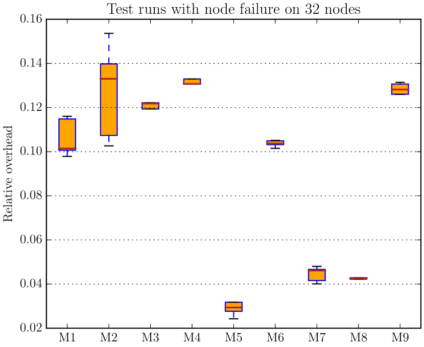
Figure 2: Relative runtime overheads when simulating a node failure and reconstructing the state of the solver, compared to the non-resilient case

Table 1: Properties of the test matrices

ID	Name	Size $n$	Non-zeros
M1	bcsstk18	$11\,948$	$149\,090$
M2	s1rmt3m1	$5489$	$217\,651$
M3	s1rmq4m1	$5489$	$262\,411$
M4	bcsstk17	$10\,974$	$428\,650$
M5	parabolic_fem	$525\,825$	$3\,674\,625$
M6	offshore	$259\,789$	$4\,242\,673$
M7	G3_circuit	$1\,585\,478$	$7\,660\,826$
M8	Emilia_923	$923\,136$	$40\,373\,538$
M9	Hook_1498	$1\,498\,023$	$59\,374\,451$

5.2 Implementation and experimental setup

We implemented the parallel PPCG algorithm in C, using the GNU Scientific Library (GSL) to store data structures like vectors and matrices, and MPI for parallelization. In our experiments we used GSL 2.5, Intel MPI 2018 Update 4, and OpenBLAS 0.3.5 for BLAS operations with GSL. We compiled with the Intel C compiler 18.0.5 with compiler flag -O3.

The convergence criterion for our solver is a reduction of the relative residual norm by a factor of $10^{-8}$. For solving the local linear systems during the reconstruction phase, we used a factor of $10^{-11}$ as convergence criterion. As suggested by Ghysels and Vanroose [32], our PPCG implementation provides the opportunity to perform residual replacement to improve the accuracy of the result. In all of our test runs, residual replacement was performed every 50 iterations (this value is also used in [32]).

Our experiments were executed on 32 nodes of the “Hydra” cluster situated at TU Wien. We used one process per node, which is sufficient to obtain representative results for the reconstruction phase.

Table 2: Experimental results

ID	$t_{0}$ [s]	Iterations until	Relative overhead with	Iterations until convergence	Relative overhead
		convergence	redundant copies [%]	if node failure occurs	with node failure [%]
M1	$0.09$	$1551$	$0.21$	$1550$	$10.14$
M2	$0.03$	$741$	$-0.07$	$742$	$13.30$
M3	$0.03$	$673$	$0.11$	$674$	$12.18$
M4	$0.16$	$2531$	$-0.37$	$2669$	$13.07$
M5	$4.61$	$2554$	$1.38$	$2554$	$2.94$
M6	$2.80$	$1948$	$1.19$	$1950$	$10.37$
M7	$15.39$	$3097$	$1.83$	$3097$	$4.61$
M8	$47.18$	$10\,227$	$-0.02$	$10\,229$	$4.26$
M9	$35.46$	$4703$	$0.04$	$4703$	$12.81$

For each matrix, three different sets of test runs were executed. The first set solves the linear system with the non-resilient standard PPCG algorithm. In the second set, our strategy for guaranteed data redundancy (cf. LABEL:Sectionsecredundancy) is used, but no node failure occurs during the run. Finally, in the last set, a node failure is simulated and the state of the solver is reconstructed as described in LABEL:Sectionsecrecovery:ppcg and LABEL:Algorithmalgesrppcg. Node failures are introduced after 50% of the solver progress (i.e., after 50% of the iterations the solver needs to converge for a particular matrix if no failure occurs) and are always simulated at the node with rank 0.

All time measurements shown in the following are averaged over five test runs. They only represent the time needed from the start of the iterative solver until convergence, ignoring the time needed for setup operations such as reading the matrix from a file or creating the preconditioner. Similarly, for the test runs with reconstruction, the measured overheads concern the time needed for the recovery of the lost vectors and scalars. The reloading of the system matrix and the preconditioner on the replacement node is excluded from the time measurements, since this would also be necessary for any other approach (like checkpointing) and, therefore, does not provide any information about the performance of our specific method.

5.3 Results

LABEL:Tabletabexperiments:results summarizes the experimental results for our nine test matrices. The runtime for executing the non-resilient standard PPCG solver is denoted as $t_{0}$. The relative overheads with respect to $t_{0}$ are listed in LABEL:Tabletabexperiments:results and visualized as boxplots in Figures 1 and 2, showing the case without and with node failures, respectively. Note that the number of iterations until convergence marginally varies between the two cases. This is due to numerical effects during the reconstruction phase, which may cause the reconstructed state of the solver to slightly deviate from the state before the node failure, thus leading to a different subsequent behavior of the solver.

We observe almost negligible relative overheads of well below 3% for all our test runs with additional data redundancy but without any node failures. For the test runs with pure band matrices (M1–M4, M8, and M9), the overheads even are within $\pm 1\%$, which can be explained with system effects. This indicates that overlapping the global dot product with the SpMV (including the additional data redundancy) indeed works best for banded matrices. Hence, our data redundancy strategy (as outlined in LABEL:Sectionsecredundancy) can be considered a particularly good fit for the PPCG solver, which has been primarily designed for band matrices (cf. LABEL:Sectionsecexperiments:data).

The relative overheads of approximately 3% to 13% for the test runs with node failures are in a similar range as previous results for recovering from a node failure in the context of the classical (non-pipelined) PCG solver [46]. This demonstrates the efficiency of our novel recovery algorithm for the PPCG method.

6 Conclusions

In this paper, we first reviewed three existing communication-hiding and thus scalable variants of the PCG and PCR algorithms. We then proposed an extension to these algorithms in order to make them resilient against the potential failure of compute nodes without compromizing the scalability of the algorithms. In fact, the improved resilience may even have positive effects on the scalability for massively parallel systems. Our experimental evaluation of the PPCG algorithm illustrates that the overheads caused by ensuring resilience against potential node failures and by reconstructing the state of the solver after a node failure are very low: almost negligible in the failure-free scenario and between 3% and 13% when a node fails. In future work, we want to experimentally investigate the behavior of our resilient pipelined PCG solvers on large-scale parallel systems.

References

- [1] E. Agullo, S. Cools, E. Fatih-Yetkin, L. Giraud, and W. Vanroose, On soft errors in the conjugate gradient method: sensitivity and robust numerical detection, Tech. Rep. RR-9226, Inria, 2018.
- [2] E. Agullo, L. Giraud, A. Guermouche, J. Roman, and M. Zounon, Towards resilient parallel linear Krylov solvers: recover-restart strategies, Tech. Rep. RR-8324, Inria, 2013.
- [3] E. Agullo, L. Giraud, A. Guermouche, J. Roman, and M. Zounon, Numerical recovery strategies for parallel resilient Krylov linear solvers, Numerical Linear Algebra with Applications, 23 (2016), pp. 888–905.
- [4] S. Balay, W. D. Gropp, L. C. McInnes, and B. F. Smith, Efficient management of parallelism in object-oriented numerical software libraries, in Modern software tools for scientific computing, Springer, 1997, pp. 163–202.
- [5] S. Balay et al., PETSc users manual, Tech. Rep. ANL-95/11 - Revision 3.11, Argonne National Laboratory, 2019.
- [6] R. Barrett, M. W. Berry, T. F. Chan, J. Demmel, J. Donato, J. Dongarra, V. Eijkhout, R. Pozo, C. Romine, and H. Van der Vorst, Templates for the solution of linear systems: building blocks for iterative methods, vol. 43, SIAM, 1994.
- [7] W. Bland, A. Bouteiller, T. Herault, G. Bosilca, and J. Dongarra, Post-failure recovery of MPI communication capability: Design and rationale, The International Journal of High Performance Computing Applications, 27 (2013), pp. 244–254.
- [8] G. Bosilca, A. Bouteiller, T. Herault, Y. Robert, and J. Dongarra, Assessing the impact of ABFT and checkpoint composite strategies, in 2014 IEEE International Parallel & Distributed Processing Symposium Workshops, IEEE, 2014, pp. 679–688.
- [9] , Composing resilience techniques: ABFT, periodic and incremental checkpointing, International Journal of Networking and Computing, 5 (2015), pp. 2–25.
- [10] G. Bronevetsky and B. de Supinski, Soft error vulnerability of iterative linear algebra methods, in Proceedings of the 22nd annual international conference on Supercomputing, ACM, 2008, pp. 155–164.
- [11] E. C. Carson, The adaptive s-step conjugate gradient method, SIAM Journal on Matrix Analysis and Applications, 39 (2018), pp. 1318–1338.
- [12] E. C. Carson, M. Rozloznik, Z. Strakos, P. Tichy, and M. Tůma, The numerical stability analysis of pipelined conjugate gradient methods: Historical context and methodology, SIAM Journal on Scientific Computing, 40 (2018), pp. A3549–A3580.
- [13] Z. Chen, Algorithm-based recovery for iterative methods without checkpointing, in Proceedings of the 20th International Symposium on High Performance Distributed Computing, ACM, 2011, pp. 73–84.
- [14] A. T. Chronopoulos and C. W. Gear, s-step iterative methods for symmetric linear systems, Journal of Computational and Applied Mathematics, 25 (1989), pp. 153–168.
- [15] S. Cools, Numerical analysis of the maximal attainable accuracy in communication hiding pipelined conjugate gradient methods, arXiv preprint arXiv:1804.02962, (2018).
- [16] S. Cools, J. Cornelis, P. Ghysels, and W. Vanroose, Improving strong scaling of the conjugate gradient method for solving large linear systems using global reduction pipelining, arXiv preprint arXiv:1905.06850, (2019).
- [17] S. Cools, J. Cornelis, and W. Vanroose, Numerically stable recurrence relations for the communication hiding pipelined conjugate gradient method, IEEE Transactions on Parallel and Distributed Systems, (2019).
- [18] S. Cools and W. Vanroose, Numerically stable variants of the communication-hiding pipelined conjugate gradients algorithm for the parallel solution of large scale symmetric linear systems, arXiv preprint arXiv:1706.05988, (2017).
- [19] S. Cools, W. Vanroose, E. F. Yetkin, E. Agullo, and L. Giraud, On rounding error resilience, maximal attainable accuracy and parallel performance of the pipelined conjugate gradients method for large-scale linear systems in PETSc, in Proceedings of the Exascale Applications and Software Conference 2016, ACM, 2016, p. 3.
- [20] S. Cools, E. F. Yetkin, E. Agullo, L. Giraud, and W. Vanroose, Analyzing the effect of local rounding error propagation on the maximal attainable accuracy of the pipelined conjugate gradient method, SIAM Journal on Matrix Analysis and Applications, 39 (2018), pp. 426–450.
- [21] J. Cornelis, S. Cools, and W. Vanroose, The communication-hiding conjugate gradient method with deep pipelines, arXiv preprint arXiv:1801.04728, (2018).
- [22] T. A. Davis and Y. Hu, The University of Florida sparse matrix collection, ACM Transactions on Mathematical Software, 38 (2011), pp. 1:1–1:25.
- [23] E. F. D’Azevedo, V. Eijkhout, and C. H. Romine, LAPACK working note 56: Reducing communication costs in the conjugate gradient algorithm on distributed memory multiprocessor, tech. rep., University of Tennessee, 1993.
- [24] E. F. D’Azevedo and C. H. Romine, Reducing communication costs in the conjugate gradient algorithm on distributed memory multiprocessors, tech. rep., Oak Ridge National Laboratory, 1992.
- [25] E. De Sturler and H. A. van der Vorst, Reducing the effect of global communication in GMRES (m) and CG on parallel distributed memory computers, Applied Numerical Mathematics, 18 (1995), pp. 441–459.
- [26] J. W. Demmel, M. T. Heath, and H. A. Van Der Vorst, Parallel numerical linear algebra, Acta numerica, 2 (1993), pp. 111–197.
- [27] K. Dichev and D. S. Nikolopoulos, TwinPCG: Dual thread redundancy with forward recovery for preconditioned conjugate gradient methods, in 2016 IEEE International Conference on Cluster Computing (CLUSTER), IEEE, 2016, pp. 506–514.
- [28] V. Eijkhout, LAPACK working note 51: Qualitative properties of the conjugate gradient and Lanczos methods in a matrix framework, tech. rep., University of Tennessee, 1992.
- [29] P. R. Eller and W. Gropp, Scalable non-blocking preconditioned conjugate gradient methods, in Proceedings of the International Conference for High Performance Computing, Networking, Storage and Analysis, IEEE Press, 2016, p. 18.
- [30] M. Fasi, J. Langou, Y. Robert, and B. Uçar, A backward/forward recovery approach for the preconditioned conjugate gradient method, Journal of Computational Science, 17 (2016), pp. 522–534.
- [31] P. Ghysels, T. J. Ashby, K. Meerbergen, and W. Vanroose, Hiding global communication latency in the GMRES algorithm on massively parallel machines, SIAM Journal on Scientific Computing, 35 (2013), pp. C48–C71.
- [32] P. Ghysels and W. Vanroose, Hiding global synchronization latency in the preconditioned conjugate gradient algorithm, Parallel Computing, 40 (2014), pp. 224–238.
- [33] L. Grigori, S. Moufawad, and F. Nataf, Enlarged Krylov subspace conjugate gradient methods for reducing communication, SIAM Journal on Matrix Analysis and Applications, 37 (2016), pp. 744–773.
- [34] T. Herault and Y. Robert, Fault-tolerance techniques for high-performance computing, Springer, 2015.
- [35] M. R. Hestenes and E. Stiefel, Methods of conjugate gradients for solving linear systems, vol. 49, NBS, 1952.
- [36] T. Hoefler, T. Schneider, and A. Lumsdaine, LogGOPSim: simulating large-scale applications in the LogGOPS model, in Proceedings of the 19th ACM International Symposium on High Performance Distributed Computing, ACM, 2010, pp. 597–604.
- [37] M. Hoemmen, Communication-avoiding Krylov subspace methods, PhD thesis, UC Berkeley, 2010.
- [38] Y. Idomura, T. Ina, S. Yamashita, N. Onodera, S. Yamada, and T. Imamura, Communication avoiding multigrid preconditioned conjugate gradient method for extreme scale multiphase CFD simulations, in 2018 IEEE/ACM 9th Workshop on Latest Advances in Scalable Algorithms for Large-Scale Systems (scalA), IEEE, 2018, pp. 17–24.
- [39] J. Langou, Z. Chen, G. Bosilca, and J. Dongarra, Recovery patterns for iterative methods in a parallel unstable environment, SIAM Journal on Scientific Computing, 30 (2007), pp. 102–116.
- [40] A. Mayumi, Y. Idomura, T. Ina, S. Yamada, and T. Imamura, Left-preconditioned communication-avoiding conjugate gradient methods for multiphase CFD simulations on the K computer, in 2016 7th Workshop on Latest Advances in Scalable Algorithms for Large-Scale Systems (ScalA), IEEE, 2016, pp. 17–24.
- [41] Message Passing Interface Forum, MPI: A message-passing interface standard. https://www.mpi-forum.org/docs/, 2015.
- [42] , User level failure mitigation. http://fault-tolerance.org/, 2017.
- [43] G. Meurant, Multitasking the conjugate gradient method on the CRAY X-MP/48, Parallel Computing, 5 (1987), pp. 267–280.
- [44] C. Pachajoa and W. N. Gansterer, On the resilience of conjugate gradient and multigrid methods to node failures, in European Conference on Parallel Processing, Springer, 2017, pp. 569–580.
- [45] C. Pachajoa, M. Levonyak, and W. N. Gansterer, Extending and evaluating fault-tolerant preconditioned conjugate gradient methods, in 2018 IEEE/ACM 8th Workshop on Fault Tolerance for HPC at eXtreme Scale (FTXS), IEEE, 2018, pp. 49–58.
- [46] C. Pachajoa, M. Levonyak, W. N. Gansterer, and J. L. Träff, How to make the preconditioned conjugate gradient method resilient against multiple node failures, in Proceedings of the 48th International Conference on Parallel Processing, ACM, 2019, pp. 67:1–67:10.
- [47] Y. Saad, Practical use of some Krylov subspace methods for solving indefinite and nonsymmetric linear systems, SIAM Journal on Scientific and Statistical Computing, 5 (1984), pp. 203–228.
- [48] Y. Saad, Iterative methods for sparse linear systems, SIAM, 2nd ed., 2003.
- [49] P. Sanan, S. M. Schnepp, and D. A. May, Pipelined, flexible Krylov subspace methods, SIAM Journal on Scientific Computing, 38 (2016), pp. C441–C470.
- [50] P. Sao and R. Vuduc, Self-stabilizing iterative solvers, in Proceedings of the Workshop on Latest Advances in Scalable Algorithms for Large-Scale Systems, ACM, 2013, p. 4.
- [51] M. Shantharam, S. Srinivasmurthy, and P. Raghavan, Fault tolerant preconditioned conjugate gradient for sparse linear system solution, in Proceedings of the 26th ACM international conference on Supercomputing, ACM, 2012, pp. 69–78.
- [52] D. Tiwari, S. Gupta, and S. S. Vazhkudai, Lazy checkpointing: Exploiting temporal locality in failures to mitigate checkpointing overheads on extreme-scale systems, in 2014 44th Annual IEEE/IFIP International Conference on Dependable Systems and Networks, IEEE, 2014, pp. 25–36.