Duality and Transport for Supersymmetric Graphene from the Hemisphere Partition Function

Abstract

We use localization to compute the partition function of a four dimensional, supersymmetric, abelian gauge theory on a hemisphere coupled to charged matter on the boundary. Our theory has eight real supercharges in the bulk of which four are broken by the presence of the boundary. The main result is that the partition function is identical to that of ${\mathcal{N}}=2$ abelian Chern-Simons theory on a three-sphere coupled to chiral multiplets, but where the quantized Chern-Simons level is replaced by an arbitrary complexified gauge coupling $\tau$. The localization reduces the path integral to a single ordinary integral over a real variable. This integral in turn allows us to calculate the scaling dimensions of certain protected operators and two-point functions of abelian symmetry currents at arbitrary values of $\tau$. Because the underlying theory has conformal symmetry, the current two-point functions tell us the zero temperature conductivity of the Lorentzian versions of these theories at any value of the coupling. We comment on S-dualities which relate different theories of supersymmetric graphene. We identify a couple of self-dual theories for which the complexified conductivity associated to the U(1) gauge symmetry is $\tau/2$.

1 Introduction

The theory of a four dimensional photon interacting with charged matter on a three dimensional boundary or interface possesses a number of remarkable properties. Studied a number of years ago in the context of D-brane physics, graphene, and toy models of confinement Gorbar:2001qt ; Reystalk ; Kaplan:2009kr , the model has had an increasing impact on the literature in recent years. See refs. Grignani:2019zxc ; Hsiao:2018fsc ; Hsiao:2017lch ; Teber:2018jdh ; DiPietro:2019hqe ; Herzog:2017xha for more recent works on this theory. Our work here is an application of a supersymmetric version Herzog:2018lqz of this theory.

We compute the partition function on a four dimensional hemisphere $HS^{4}$ using localization techniques. While this particular localization calculation has to our knowledge not been performed, it relies heavily on earlier results. We take advantage of previous localization calculations on $S^{4}$ Pestun:2007rz ; Hama:2012bg and on $S^{3}$ Hama:2011ea ; Hama:2010av ; Kapustin:2009kz . There is even a closely related localization calculation for a non-abelian gauge theory on $HS^{4}$ Gava:2016oep . Ref. Gava:2016oep is in one respect more general than our case, but in another not general enough. While ref. Gava:2016oep focuses on nonabelian gauge theory, our theory is abelian. While ref. Gava:2016oep restricts to Neumann or Dirichlet conditions for the gauge field, the novel ingredient in our work is that we allow dynamical degrees of freedom on the boundary to couple to the bulk gauge field. In particular, we allow for $n_{+}$ and $n_{-}$ oppositely charged chiral multiplets.

One remarkable feature of this graphene-like theory is that the complexified gauge coupling,

$$\tau\equiv\frac{2\pi\mathrm{i}}{g^{2}}+\frac{\theta}{2\pi}\,,$$ (1)

is exactly marginal Teber:2018jdh ; Herzog:2017xha ; Dudal:2018pta ; Herzog:2018lqz . Thus we have an example of a boundary (or interface) conformal field theory for all values of $\tau$. Localization provides a method for determining the dependence of the partition function on $\tau$ and studying precisely how the theory may change as a function of this coupling. As emphasized in ref. DiPietro:2019hqe , at certain special values of the complexified coupling, associated with cusps in the action of $SL(2,{\mathbb{Z}})$ on $\tau$, the boundary theory “decouples” from the bulk and becomes three dimensional. At these values, the complexified coupling $\tau$ is reinterpreted as a quantized – either integer or half-integer – Chern-Simons level $k$. Our partition function reduces to that of abelian Chern-Simons theory on a three sphere. Indeed, our main result is that our hemisphere partition function is identical to the three sphere ${\mathcal{N}}=2$ abelian Chern-Simons theory partition function (with matter) with the replacement of $\tau$ for $k$.

Our hemisphere partition function (73) takes the form of a single definite integral over a function involving dilogarithms. In addition to the complexified coupling $\tau$, the integral depends on a number of potentials $q_{i}$ which control the mixing of the R-symmetry with other U(1) symmetries in the theory. In analogy with the arguments for 3d Chern-Simons theories Jafferis:2010un ; Closset:2012vg , we expect conformal symmetry picks out special values $q_{i}^{*}$ which minimize the absolute value of the partition function $|Z|$. The vanishing of $\partial_{q_{i}}|Z|$ correlates with the vanishing of certain one point functions of boundary operators, while the positivity of $\partial_{q_{i}}\partial_{q_{j}}|Z|$ means certain boundary two point functions are reflection positive.

While we cannot evaluate the partition function integral in general, we can analyze it in a variety of limits. We use the saddle point approximation to extract results both at large $|\tau|$ and large $n$. In the decoupling limit $\tau=k$, we use contour integration to reduce the integral to a sum over residues Garoufalidis:2014ifa . We also use this same contour integration technique to perform an S duality on our integral, $\tau\to-1/\tau$. We identify a couple of theories which have self dual points.

Interestingly, we are able to compute quantities associated with transport in our theory. A second derivative of our partition function with respect to the $q_{i}$ gives us two-point functions of U(1) currents Closset:2012vg . As our theories are conformal, we can map these current-current two-point functions from the sphere back to flat space. A Kubo formula then relates these two-point functions to associated conductivities. Through self duality, we can also establish the conductivity with respect to the U(1) gauge symmetry has a particularly simple form at self dual points, namely $2\pi(\sigma_{H}+\mathrm{i}\sigma)=\tau/2$ in our two examples. In the condensed matter context, this “quantum conductivity” has been associated with the conductivity at quantum critical points, for example the conductivity of a metallic thin film at a superfluid insulator transition Fisher:1990zza ; Wen:1990gi or the conductivity of a quantum Hall system at the transition between two plateaux Engel:1993zz ; Shahar:1997zz . Note in our system, we have access to the conductivities at arbitrary coupling, not just perturbatively where there is expected to be a quasiparticle interpretation. Additionally, we know precisely what the field theory interpretation is, unlike for example in certain bottom-up holographic models in AdS/CFT.

An outline of the manuscript follows. In section 2, we discuss supersymmetry preserving boundary conditions in our Euclidean framework. In section 3, we review Killing spinors on $S^{4}$. Section 4 contains the action for our graphene-like theory. Section 5 presents the localization calculation and introduces two techniques to analyze the resulting integral: saddle point approximation and a contour integration. Finally, section 6 presents the results on S duality and transport. We conclude with a brief discussion in section 7. Appendix A presents our conventions for fermions while appendix B gives some results for the partition function in simple special cases. Readers not interested in the details of the localization calculation may wish to stare briefly at the definition of the theory (47), (51), and (63) before proceeding directly to section 5.

2 Supersymmetry and Boundary Conditions

Two facts about supersymmetry greatly constrain our problem. The first is that most of the localization technology available requires the existence of a continuous R-symmetry. The second is that the presence of a boundary will break at least half of the supersymmetry present in the bulk, because supercharges square to translation generators. The simplest theory we may consider in 4d should thus have at least ${\mathcal{N}}=2$ supersymmetry with (in more familiar Lorentzian signature) $SU(2)\times U(1)$ R-symmetry. The boundary will have 3d ${\mathcal{N}}=2$ supersymmetry and preserve only a diagonal $U(1)\subset SU(2)$ of the bulk R-symmetry.

Let us see how this breaking works at the level of the supersymmetry algebra. For 4d ${\mathcal{N}}=2$ SUSY, it is convenient to introduce symplectic Majorana fermions which have a charge conjugation condition

$$\overline{Q}_{i}=\varepsilon_{ij}Q^{jT}C\ ,$$ (2)

where $\gamma^{\mu T}=C\gamma^{\mu}C^{-1}$. (See appendix A for our conventions.) The relevant part of the ${\mathcal{N}}=2$ algebra is given by

$$\{Q^{i},\overline{Q}_{j}\}=2\mathrm{i}\delta^{i}_{j}{\not{\rm D}}\,,$$ (3)

where $iD_{\mu}$ generates translation in 4 dimensions. The $Q_{i}$ transform as a doublet under the $SU(2)$ R-symmetry and via $Q_{i}\to e^{\eta\gamma^{5}}Q_{i}$ under the additional $U(1)$. As we work in Euclidean signature, $\eta$ is a real parameter, and the symmetry is not a compact $U(1)$ but actually $SO(1,1)$.

The presence of a boundary breaks translation invariance in the normal direction. We are thus looking for a subalgebra which generates only translations along the boundary, $\mathrm{i}{\rm D}_{A}$. We can define this subalgebra through projectors $\Pi_{\pm}{}^{i}{}_{j}$ that preserve the tangential gamma matrices Herzog:2018lqz :

$${\Pi_{+}}^{i}{}_{k}\gamma^{\mu}{\overline{\Pi}_{+}}^{k}{}_{j}=\delta^{\mu}_{A}{\Pi_{+}}^{i}{}_{j}\gamma^{A}\ .$$ (4)

The definition of $\overline{\Pi}_{\pm}$ is induced from the definition of the symplectic Majorana condition (2):

$${{\overline{\Pi}_{\pm}}^{j}}_{i}=-C^{-1}\varepsilon^{jk}{(\Pi^{T}_{\pm})_{k}}^{l}\varepsilon_{li}C\ .$$ (5)

The projectors satisfy the usual properties $\Pi_{+}+\Pi_{-}=1$ and $\Pi_{+}\Pi_{-}=0$. From (4) follow the relations

$${\overline{\Pi}_{\pm}}^{i}{}_{j}\gamma^{A}=\gamma^{A}{\Pi_{\pm}}^{i}{}_{j}\ ,\;\;\;{\overline{\Pi}_{\pm}}^{i}{}_{j}\gamma^{n}=\gamma^{n}{\Pi_{\mp}}^{i}{}_{j}\ ,\;\;\;{\Pi_{\pm}}^{i}{}_{j}\gamma^{5}=\gamma^{5}{\Pi_{\mp}}^{i}{}_{j}\ .$$ (6)

Projectors satisfying our conditions are

$${\Pi_{\pm}}^{i}_{j}=\frac{1}{2}(\delta^{i}_{j}\pm\mathrm{i}\vec{v}\cdot{\vec{\tau}}^{i}{}_{j}\,\gamma^{5}\gamma^{n}e^{\eta\gamma^{5}})\ .$$ (7)

The vector $\vec{\tau}=(\sigma_{1},\sigma_{2},\sigma_{3})$ of Pauli spin matrices generates the $SU(2)$ R-symmetry, while $\vec{v}$ is a unit vector which determines how the $SU(2)$ is broken down to a $U(1)$ subgroup by the boundary. The $\eta$ parameter similarly determines how the bulk $SO(1,1)$ R-symmetry is broken. The 3d supersymmetry algebra we take to be generated by ${\Pi_{+}}^{i}{}_{j}Q^{j}$.

One caveat to obtain this projection is that the analysis is not for the general curved space but for the flat space. As the projector $\Pi_{\pm}{}^{i}_{j}$ is not covariantly constant, the projected generator ${\Pi_{+}}^{i}{}_{j}Q^{j}$ is not in general a symmetry generator or, equivalently, the corresponding projected spinor ${\Pi_{+}}^{i}{}_{j}\xi^{j}$ is not the Killing spinor. Thus the algebra (3) will not be simply projected to its tangential direction . However, at the boundary of our example $HS^{4}$, the projector will be covariantly constant as there is no spin connection along the normal direction and no mixing between normal and tangential directions. The projected spinor at the boundary is the $3d$ Killing spinor, projecting the algebra (3) to its tangential direction. Therefore, we can use the projector (7) for our example.

For simplicity, in what follows we take $\vec{v}=(0,0,1)$ and $\eta=0$. As ${\Pi_{\pm}}^{i}_{j}$ becomes diagonal in the SU(2) basis, it is convenient to identify projectors associated with each basis element:

$${(\Pi_{+})^{1}}_{1}=\pi_{+}\ ,\;\;\;{(\Pi_{+})^{2}}_{2}=\pi_{-}\ \;\;\;\mbox{where }\pi_{\pm}=\frac{1}{2}(1\pm\mathrm{i}\gamma^{5}\gamma^{n})\ .$$ (8)

Another simplification is that ${\overline{\Pi}_{\pm}}^{i}{}_{j}={\Pi_{\pm}}^{i}_{j}$. Because the $\gamma^{A}$ commute with ${\Pi_{\pm}}^{i}_{j}$ (6), we can use the tangential 4d gamma matrices $\gamma^{A}$ to generate our 3d gamma matrix algebra:

$$\Gamma^{A}=\pi_{+}\gamma^{A}\ .$$ (9)

The projection ${\Pi_{+}}^{i}_{j}Q^{j}$ can be broken down into components

$${(\Pi_{+})^{1}}_{1}Q^{1}=\pi_{+}Q^{1}\equiv Q_{+}\ ,\;\;\;{(\Pi_{+})^{2}}_{2}Q^{2}=\pi_{-}Q^{2}\equiv\gamma^{n}Q_{+}^{\prime}\ .$$ (10)

The charge conjugation matrix in 3d needs to be altered slightly from its 4d version:

$$\widetilde{C}=C\gamma^{n}\ .$$ (11)

The extra $\gamma^{n}$ ensures that $\widetilde{C}\pi_{\pm}=\pi_{\pm}^{T}\widetilde{C}$. The alteration leads to some sign differences in 3d, e.g. $\widetilde{C}\Gamma^{A}\widetilde{C}^{-1}=-(\Gamma^{A})^{T}$. With the new charge conjugation matrix $\widetilde{C}$ in hand, we define the 3d barred spinors as

$$\widetilde{Q}_{+}=Q_{+}^{T}\widetilde{C}\ .$$ (12)

The 4d symplectic Majorana condition (2) implies a 3d symplectic Majorana condition

$$Q_{+}^{\dagger}=\widetilde{Q}^{\prime}_{+}\ ,\;\;\;Q^{\prime\dagger}_{+}=-\widetilde{Q}_{+}\ .$$ (13)

3 Killing Spinors on Spheres

On a curved manifold, the supersymmetry is generated by Killing spinors. One of our first chores is then to work out the Killing spinors on $HS^{4}$ and determine which ones are compatible with the boundary conditions imposed by the projector $\Pi_{+}$.

We can write a metric on $S^{4}$,

$${\rm d}s^{2}=\frac{\sin^{2}r}{4}\left[\sin^{2}\theta\,{\rm d}\phi^{2}+{\rm d}\theta^{2}+({\rm d}\psi+\cos\theta\,{\rm d}\phi)^{2}\right]+{\rm d}r^{2}\ .$$ (14)

The hemisphere $HS^{4}$ comes from restricting the range of the polar angle to $0\leq r\leq\frac{\pi}{2}$. We introduce the vielbeins

$$e^{\phi} = \frac{\sin r}{2}\sin\theta\,{\rm d}\phi\ ,\;\;\;e^{\theta}=\frac{\sin r}{2}{\rm d}\theta\ ,$$

$$e^{\psi} = \frac{\sin r}{2}({\rm d}\psi+\cos\theta\,{\rm d}\phi)\ ,\;\;\;e^{r}={\rm d}r\ .$$ (15)

where we are implicitly assuming an ordering of the gamma matrices, associating $\gamma^{1}$ with $e^{\phi}$, $\gamma^{2}$ with $e^{\theta}$, $\gamma^{3}$ with $e^{\psi}$ and most importantly $\gamma^{4}$ or $\gamma^{n}$ with $e^{r}$. These vielbeins give the following connection one form:

$${\omega^{\psi}}_{r} =\cot r\,e^{\psi}\ ,$$

$${\omega^{\theta}}_{r} =\cot r\,e^{\theta}\ , {\omega^{\theta}}_{\psi} =\frac{1}{\sin r}e^{\phi}$$ (16)

$${\omega^{\phi}}_{r} =\cot r\,e^{\phi}\ , {\omega^{\phi}}_{\psi} =-\frac{1}{\sin r}e^{\theta}\ , {\omega^{\phi}}_{\theta} =\frac{1}{\sin r}\left(2\cot\theta\,e^{\phi}-e^{\psi}\right)\ .$$

We look for solutions of the Killing spinor equations

$${\rm D}_{\mu}\psi=\pm\frac{\mathrm{i}}{2}\gamma_{\mu}\psi\ .$$ (17)

There are eight solutions

$$\psi^{(1)}_{\pm} =\left(\begin{array}[]{c}\cos\frac{r}{2}\\ 0\\ \pm\mathrm{i}\sin\frac{r}{2}\\ 0\end{array}\right)e^{\mathrm{i}\psi/2}\ ,\;\;\; \psi^{(2)}_{\pm} =\left(\begin{array}[]{c}0\\ \cos\frac{r}{2}\\ 0\\ \pm\mathrm{i}\sin\frac{r}{2}\end{array}\right)e^{-\mathrm{i}\psi/2}\ ,$$ (26)

$$\chi^{(1)}_{\pm} =\left(\begin{array}[]{c}\sin\frac{r}{2}\sin\frac{\theta}{2}\\ -\sin\frac{r}{2}\cos\frac{\theta}{2}\\ \mp\mathrm{i}\cos\frac{r}{2}\sin\frac{\theta}{2}\\ \pm\mathrm{i}\cos\frac{r}{2}\cos\frac{\theta}{2}\end{array}\right)e^{\mathrm{i}\phi/2}\ ,\;\;\; \chi^{(2)}_{\pm} =\left(\begin{array}[]{c}\sin\frac{r}{2}\cos\frac{\theta}{2}\\ \sin\frac{r}{2}\sin\frac{\theta}{2}\\ \mp\mathrm{i}\cos\frac{r}{2}\cos\frac{\theta}{2}\\ \mp\mathrm{i}\cos\frac{r}{2}\sin\frac{\theta}{2}\end{array}\right)e^{-\mathrm{i}\phi/2}\ .$$ (35)

The spinors satisfy the following reality conditions

$$\psi_{\mp}^{(2)}=C\psi_{\pm}^{(1)*}\ ,\;\;\;\chi_{\mp}^{(2)}=C\chi_{\pm}^{(1)*}\,,$$ (36)

which allows us to repackage them into eight sets of symplectic Majorana spinors $\xi^{i}_{a}$ as

$$\begin{array}[]{ll}\xi_{1}^{i}\;=\;\bigl{(}\chi^{(1)}_{+}\,,\chi^{(2)}_{-}\bigr{)}\,,{}{}&\xi_{2}^{i}\;=\;\bigl{(}\mathrm{i}\chi^{(1)}_{+}\,,-\mathrm{i}\chi^{(2)}_{-}\bigr{)}\,,\\ \xi_{3}^{i}\;=\;\bigl{(}\mathrm{i}\chi^{(2)}_{+}\,,\mathrm{i}\chi^{(1)}_{-}\bigr{)}\,,{}{}&\xi_{4}^{i}\;=\;\bigl{(}\chi^{(2)}_{+}\,,-\chi^{(1)}_{-}\bigr{)}\,,\\ \xi_{5}^{i}\;=\;\bigl{(}\psi^{(1)}_{+}\,,\psi^{(2)}_{-}\bigr{)}\,,{}{}&\xi_{6}^{i}\;=\;\bigl{(}\mathrm{i}\psi^{(1)}_{+}\,,-\mathrm{i}\psi^{(2)}_{-}\bigr{)}\,,\\ \xi_{7}^{i}\;=\;\bigl{(}\mathrm{i}\psi^{(2)}_{+}\,,\mathrm{i}\psi^{(1)}_{-}\bigr{)}\,,{}{}{}{}&\xi_{8}^{i}\;=\;\bigl{(}\psi^{(2)}_{+}\,,-\psi^{(1)}_{-}\bigr{)}\,,\end{array}$$ (37)

that are orthonormal to each other as $\overline{\xi_{ai}}\xi^{i}_{b}=2\delta_{ab}$. The Killing spinor condition on these symplectic Majorana fermions becomes

$${\rm D}_{\mu}\xi^{i}_{a}=\frac{\mathrm{i}}{2}\gamma_{\mu}{(\tau_{3})^{i}}_{j}\xi^{j}_{a}\ .$$ (38)

The spinors $\xi^{i}_{a}\,,a=1,2,3,4$ generate a Killing vector in the $\phi$ direction while the spinors $\xi^{i}_{a}\,,a=5,6,7,8$ generate a Killing vector in the $\psi$ direction,

$$\begin{array}[]{l}\overline{\xi_{ai}}\gamma^{\mu}\xi^{i}_{a}=(\pm 4\,,0\,,0\,,0)\,,~{}~{}~{}\mbox{+ for }a=1,2~{}~{}~{}-\mbox{ for }a=3,4,\\ \overline{\xi_{ai}}\gamma^{\mu}\xi^{i}_{a}=(0\,,0\,,\pm 4\,,0)\,,~{}~{}~{}\mbox{+ for }a=5,6~{}~{}~{}-\mbox{ for }a=7,8\,.\end{array}$$ (39)

At the equator $r=\frac{\pi}{2}$, the Killing spinors satisfy the projection conditions

$$\Pi_{-}\xi_{a}^{i}|_{r=\pi/2}=0\ , \;\;\;\mbox{for }a=1,2,3,4\,,$$ (40)

$$\Pi_{+}\xi_{a}^{i}|_{r=\pi/2}=0\ , \;\;\;\mbox{for }a=5,6,7,8\,.$$ (41)

We can take the preserved supersymmetry to satisfy one of the two conditions (40) and (41). On the three sphere, the Killing vectors $v^{\mu}=(1,0,0)$ for the former condition (40) and $(0,0,1)$ for the latter condition (41) are both divergenceless, ${\rm D}_{\mu}v^{\mu}=0$. While $(1,0,0)$ satisfies ${\rm D}_{\mu}v_{\nu}=-\epsilon_{\mu\nu\rho}v^{\rho}$, there is a flip in sign for $(0,0,1)$: ${\rm D}_{\mu}v_{\nu}=\epsilon_{\mu\nu\rho}v^{\rho}$.

The condition of the Killing spinors (40) (or (41)) reduces the 4-dimensional Killing spinor equation (38) to the 3-dimensional Killing spinor equation,

$${\rm D}^{(3d)}_{A}\xi_{a}^{i}=\frac{\mathrm{i}}{2}(\tau_{3})^{i}{}_{j}\gamma_{A}\xi^{j}_{a}\,,$$ (42)

at the boundary of the $HS_{4}$ where $r=\frac{\pi}{2}$. This reduction can be done because the mixing components between the normal and tangential directions of boundary in the spin connections are absent at the boundary; in fact, from (3) we see that ${\omega^{\psi}}_{r}={\omega^{\theta}}_{r}={\omega^{\phi}}_{r}=0\,$ at $r=\frac{\pi}{2}$.

4 The Action

Vector Multiplet on an $HS^{4}$

We consider the abelian vector multiplet on $HS^{4}$. In the bulk, the supersymmetry is generated by the $SU(2)$ pair of Killing spinors $(\xi^{1}\,,\xi^{2})$,

$$\delta S = \overline{\xi}_{i}\,\lambda^{i}\,,$$

$$\delta P = {\overline{\xi}}_{i}\gamma_{5}{\lambda}^{i}\,,$$

$$\delta A_{\mu} = {\overline{\xi}}_{i}\gamma_{\mu}\lambda^{i}\,,$$ (43)

$$\delta\vec{D} = \mathrm{i}\vec{\tau}^{i}{}_{j}\overline{\xi_{i}}\gamma^{a}\mathcal{D}_{a}\lambda^{j}\,,$$

$$\delta\lambda^{i} = \gamma^{a}\partial_{a}S\,{\xi}^{i}-\gamma^{a}\partial_{a}P\,\gamma_{5}{\xi}^{i}-\frac{1}{2}F_{ab}\gamma^{ab}\xi^{i}-\mathrm{i}\vec{D}\cdot\vec{\tau}^{i}{}_{j}\xi^{j}+\frac{1}{2}S\,\not{\mathcal{D}}\xi^{i}-\frac{1}{2}P\,\not{\mathcal{D}}\gamma_{5}\xi^{i}\,.$$

The supersymmetry algebra (4) squares to yield translation generators ${\mathcal{L}}_{v}$ along with other symmetry generators of the theory

$$\delta^{2}=\mathcal{L}_{v}+\text{Gauge}(\hat{\Phi})+\text{Lorentz}(L^{ab})+\text{Scale}\left({\omega}\right)+\text{R}_{SO(1,1)}({\Theta})+\text{R}_{SU(2)}(\vec{{\Theta}})\,,$$ (44)

where

$$v^{\mu}\;=\;{\overline{\xi}}_{i}\gamma^{\mu}\xi^{i}\,,~{}~{}\hat{\Phi}\;=\;{\overline{\xi}}_{i}{\xi}^{i}\,S-\overline{\xi}_{i}\gamma_{5}\xi^{i}\,P-v^{\mu}A_{\mu}\,,~{}~{}L_{ab}\;=\;\mathcal{D}_{[a}v_{b]}+v^{\mu}\omega_{\mu ab}\,,$$ (45)

$${\omega}\;=\;\frac{1}{4}\mathcal{D}_{a}v^{a}\,,~{}~{}~{}{\Theta}\;=\;-\frac{1}{2}\overline{\xi}_{i}\gamma_{5}\not{\mathcal{D}}\xi^{i}\,,~{}~{}~{}\vec{{\Theta}}\;=\;-\mathrm{i}\vec{\tau}^{j}{}_{i}\overline{\xi_{j}}\not{\mathcal{D}}\xi^{i}\,.$$

Explicitly,

$$\begin{array}[]{lll}\delta^{2}S&=&v^{\mu}\partial_{\mu}S+{\omega}S-{\Theta}P\,,\\ \delta^{2}P&=&v^{\mu}\partial_{\mu}P-{\Theta}S+{\omega}P\,,\\ \delta^{2}A_{\mu}&=&v^{\nu}F_{\nu\mu}+\partial_{\mu}{\Phi}\,,\\ \delta^{2}\lambda^{i}&=&v^{\mu}\mathcal{D}_{\mu}\lambda^{i}+\frac{3}{2}{\omega}\lambda^{i}-\frac{1}{2}{\Theta}\gamma_{5}\lambda^{i}+\frac{1}{4}\mathcal{D}_{[a}v_{b]}\gamma^{ab}\lambda^{i}+\frac{1}{2}\vec{\Theta}\cdot\vec{\tau}^{i}{}_{j}\lambda^{j}\,,\\ \delta^{2}D_{I}&=&v^{\mu}\mathcal{D}_{\mu}D_{I}+2{\omega}D_{I}+\epsilon_{IJK}\Theta_{J}D_{K}\,.\end{array}$$ (46)

The presence of the boundary of $HS^{4}$ breaks half of the supersymmetries. The supersymmetries are now generated by the four Killing spinors that satisfy the condition  (40) in terms of the projector introduced in (7). The supersymmetric action under this condition is as follows. It is divided into bulk and boundary contributions associated with the gauge coupling $g$ and theta angle $\theta$:

$$I_{V}\;=\;I_{g}+I_{\partial g}+I_{\theta}$$ (47)

$$I_{g} = \frac{1}{2g^{2}}\int_{\mathcal{M}}d^{4}x\left(\frac{1}{2}F_{\mu\nu}F^{\mu\nu}+\overline{\lambda_{i}}\not{\mathcal{D}}\lambda^{i}+(\partial_{\mu}P)^{2}-(\partial_{\mu}S)^{2}-\vec{D}^{2}+\frac{R}{6}(P^{2}-S^{2})\right),$$ (48)

$$I_{\partial g} = \int_{\partial\mathcal{M}}d^{3}x\left(-\frac{\mathrm{i}}{4}\tau_{3}{}^{i}{}_{j}\,\overline{\lambda_{i}}\gamma_{5}\lambda^{j}-P(D_{3}+\partial_{n}P)\right)\,,$$ (49)

$$I_{\theta} = \frac{\theta}{4\pi^{2}}\left[\frac{\mathrm{i}}{4}\int_{\mathcal{M}}d^{4}xF_{\mu\nu}\widetilde{F}^{\mu\nu}-\int_{\partial\mathcal{M}}d^{3}x\left(\frac{1}{2}\tau_{3}{}^{i}{}_{j}\,\overline{\lambda_{+}}_{i}\lambda^{j}_{+}-\mathrm{i}S(D_{3}+\partial_{n}P)\right)\right]\,.$$ (50)

where the masses of scalars are set by conformal coupling with the curvature of $HS^{4}$ which is taken to be $R=12$. The dual of the field strength is $\widetilde{F}^{\mu\nu}=\frac{1}{2}\epsilon^{\mu\nu\lambda\rho}F_{\lambda\rho}$. The theta angle action (50) includes the projected component of the gaugino $\lambda^{i}_{+}=\Pi_{+}{}^{i}{}_{j}\lambda^{j}$ .

One can check that the boundary term from the variation of the bulk action (48) is canceled by the variation of the boundary action (49) under the condition (40). And the action for the theta angle (50) is supersymmetric by itself. Since we are treating a $U(1)$ gauge group, we can also add the Fayet-Iliopoulos type action,

$$I_{FI} = \int_{\mathcal{M}}d^{4}x\,\left(\eta(2S+D_{3}+\partial_{n}P)\right)\,.$$ (51)

The supersymmetry variation of $2S$ is canceled by the variation of $D_{3}$ using (38), and the remaining boundary term is canceled by the variation of $\partial_{n}P$ using the projection condition (40).

The Euclidean 4-dimensional space allows the symplectic Majorana condition (2) on the spinors, giving $8$ real degrees of freedom for fermions and supercharges. The action and supersymmetry algebra are compatible with the supersymmetry transformation rules (4) if bosonic fields satisfy the following reality conditions

$$S^{\ast}=S\,,~{}~{}~{}~{}P^{\ast}=P\,,~{}~{}~{}\vec{D}^{\ast}=\vec{D}\,,~{}~{}~{}A_{\mu}^{\ast}=A_{\mu}\,.$$ (52)

However, for the quantum theory to be well defined and for the real part of the action (47) to be positive definite, we need to choose a contour in the path integral where

$$S^{\ast}=-S\,,~{}~{}~{}~{}P^{\ast}=P\,,~{}~{}~{}\vec{D}^{\ast}=-\vec{D}\,,~{}~{}~{}A_{\mu}^{\ast}=A_{\mu}\,.$$ (53)

This condition guarantees (48) is positive definite and that (49) and (50) are pure imaginary. Along this contour (53), the symplectic Majorana condition for fermions is lost. The $SU(2)$ pair of spinors are now two independent spinors, where each one has its own contour for integration. That is to say that we formally double the spinor space in Euclidean 4-dimensional space.

Supersymmetry at boundary

The boundary value of the four Killing spinors satisfying (40) defines the 3-dimensional Killing spinors. They are equivalent to the boundary value of the projected spinors $\Pi_{+}\xi^{i}$. We define the 3-dimensional boundary Killing spinors by using the simple choice of the projector (8),

$$\begin{array}[]{ll}\Pi_{+}^{1}{}_{1}\xi^{1}|_{r=\frac{\pi}{2}}=\pi_{+}\xi^{1}|_{r=\frac{\pi}{2}}\equiv\zeta_{+}\,,{}{}{}{}{}{}{}{}&\Pi_{+}^{2}{}_{2}\xi^{2}|_{r=\frac{\pi}{2}}=\pi_{-}\xi^{2}|_{r=\frac{\pi}{2}}\equiv\gamma_{n}\zeta^{\prime}_{+}\,.\end{array}$$ (54)

The 4-dimensional symplectic Majorana condition (2) leads to the 3-dimensional reality condition

$$\begin{array}[]{ll}\zeta_{+}^{\dagger}=\widetilde{{\zeta^{\prime}}_{+}}\equiv{\zeta^{\prime}_{+}}^{T}\widetilde{C}\,,{}{}{}{}{}{}{}{}&{\zeta^{\prime}}_{+}^{\dagger}=-\widetilde{\zeta_{+}}\equiv\zeta_{+}^{T}\widetilde{C}\,.\end{array}$$ (55)

However, we will not impose a reality condition and instead let $\zeta_{+}$ and $\zeta^{\prime}_{+}$ be independent spinors. For the path integral, we do not use the reality (52), but instead (53). In other words, we formally double the spinor space in Euclidean three dimensional space.

When we consider this projected supersymmetry at the boundary, the four dimensional $\mathcal{N}=2$ algebra is reduced to the three dimensional $\mathcal{N}=2$ algebra

$$\delta_{+}^{2}=\mathcal{L}_{v}+\text{Gauge}(\hat{\Phi})+\text{Lorentz}(L^{ab})+\text{Scale}\left({\omega}\right)+\text{R}_{U(1)}({\Theta}_{3})\,,$$ (56)

where the parameters (45) are reduced to

$$v^{A} = 2\,\widetilde{\zeta^{\prime}_{+}}\Gamma^{A}\zeta_{+}=2\,\widetilde{\zeta_{+}}\Gamma^{A}\zeta^{\prime}_{+}\,,~{}~{}~{}~{}~{}v^{n}=0\,,$$

$$\hat{\Phi} = 2\,\widetilde{\zeta^{\prime}_{+}}\zeta_{+}\,S-v^{A}A_{A}\,,$$

$$\omega = \frac{2}{3}\widetilde{\zeta^{\prime}_{+}}\Gamma^{A}\mathcal{D}_{A}\zeta_{+}+\frac{2}{3}\widetilde{\zeta_{+}}\Gamma^{A}\mathcal{D}_{A}\zeta^{\prime}_{+}=\frac{1}{3}\mathcal{D}_{A}v^{A}\,,$$ (57)

$${\Theta}_{3} = -\mathrm{i}\frac{4}{3}\widetilde{\zeta^{\prime}_{+}}\Gamma^{A}\mathcal{D}_{A}\zeta_{+}+\mathrm{i}\frac{4}{3}\widetilde{\zeta_{+}}\Gamma^{A}\mathcal{D}_{A}\zeta^{\prime}_{+}\ ,$$

$${\Theta} \;=\; {\Theta}_{1}\;=\;{\Theta}_{2}\;=\;0\,.$$

Note that the $SU(2)_{R}\times SO(1,1)_{R}$ R-symmetry is broken to the diagonal $U(1)_{R}$ of $SU(2)_{R}$. For the choice of the Killing spinors $\xi_{1}^{i}$ in (37), these parameters are

$$v^{A}\partial_{A}=4\partial_{\psi}\,,~{}~{}~{}\hat{\Phi}=2S-4A_{\psi}\,,~{}~{}~{}\omega=0\,,~{}~{}~{}{\Theta}_{3}=4\,.$$ (58)

In the absence of charged matter on the boundary, we may impose Dirichlet boundary conditions on $(P,A_{n},\lambda^{i}_{-},D_{1},D_{2})$ and Neumann boundary conditions on $(S,A_{A},\lambda^{i}_{+},D_{3})$ of the 4d vector multiplet fields. The nonzero fields $(S,A_{A},\lambda_{+},\lambda^{\prime}_{+},(D_{3}+\partial_{n}P))$ form a 3d vector multiplet at the boundary of $HS^{4}$, where the $\lambda_{+}$ and $\lambda^{\prime}_{+}$ are defined in the same manner as the Killing spinor (54). The supersymmetry transformation of this 3d vector multiplet takes the usual form

$$\delta_{+}A_{A} = \widetilde{\zeta^{\prime}_{+}}\Gamma_{A}\lambda_{+}+\widetilde{{\zeta_{+}}}\Gamma_{A}\lambda^{\prime}_{+}\,,$$

$$\delta_{+}\lambda_{+} = -\frac{1}{2}F_{AB}\Gamma^{AB}\zeta_{+}-\mathrm{i}(D_{3}+\partial_{n}P)\zeta_{+}+\Gamma^{A}\partial_{A}S\zeta_{+}+\frac{2}{3}S\Gamma^{A}\mathcal{D}_{A}\zeta_{+}\,,$$

$$\delta_{+}\lambda^{\prime}_{+} = -\frac{1}{2}F_{AB}\Gamma^{AB}\zeta^{\prime}_{+}+\mathrm{i}(D_{3}+\partial_{n}P)\zeta^{\prime}_{+}-\Gamma^{A}\partial_{A}S\zeta^{\prime}_{+}-\frac{2}{3}S\Gamma^{A}\mathcal{D}_{A}\zeta^{\prime}_{+}\,,$$ (59)

$$\delta_{+}(D_{3}+\partial_{n}P) = \mathrm{i}\widetilde{\zeta^{\prime}_{+}}\Gamma^{A}\mathcal{D}_{A}\lambda_{+}-\mathrm{i}\widetilde{\zeta_{+}}\Gamma^{A}\mathcal{D}_{A}\lambda_{+}^{\prime}+\mathrm{i}\frac{1}{3}\widetilde{\mathcal{D}_{A}\zeta^{\prime}_{+}}\Gamma^{A}\lambda_{+}-\mathrm{i}\frac{1}{3}\widetilde{\mathcal{D}_{A}\zeta_{+}}\Gamma^{A}\lambda^{\prime}_{+}\,,$$

$$\delta_{+}S = \widetilde{\zeta^{\prime}_{+}}\lambda_{+}-\widetilde{\zeta_{+}}\lambda^{\prime}_{+}\,.$$

Our next task, adding charged matter on the boundary, leads to a modification of these boundary conditions.

Chiral Multiplet on $S^{3}$

Next, we couple the boundary value of the vector multiplet fields with degrees of freedom living at the boundary $S^{3}$ (located at $r=\frac{\pi}{2}$). The boundary degrees of freedom consist of $n_{+}+n_{-}$ chiral multiplets, $n_{+}$ with positive gauge charge and $n_{-}$ with negative gauge charge. (Sometimes we also set $n_{+}=n_{-}=n$ to get $n$ hypermultiplets.) These chiral multiplet fields couple to the boundary modes of the bulk $U(1)$ vector multiplet. Let one of these chiral multiplets have $U(1)_{R}$ R-charge $q$. The boundary supersymmetry transformations are generated by supersymmetry parameter $\zeta^{i}_{+}$ which satisfy the algebra (56). This algebra can be realized on the chiral multiplet with the following transformations

$$\delta_{+}\phi=-2i\widetilde{\zeta}^{\prime}_{+}\psi_{+},\quad\delta_{+}\overline{\phi}=-2i\widetilde{\zeta}_{+}\psi^{\prime}_{+}\,,$$

$$\delta_{+}\psi_{+}=\mathrm{i}\Gamma^{A}\zeta_{+}\mathcal{D}_{A}\phi+\zeta_{+}S\phi-\mathrm{i}F\,\zeta^{\prime}_{+}+\mathrm{i}\frac{2}{3}q\phi\,\Gamma^{A}\mathcal{D}_{A}\zeta_{+}\,,$$

$$\delta_{+}\psi^{\prime}_{+}=\mathrm{i}\Gamma^{A}\zeta^{\prime}_{+}\mathcal{D}_{A}\overline{\phi}+\zeta^{\prime}_{+}S\overline{\phi}-\mathrm{i}\overline{F}\,\zeta_{+}+\mathrm{i}\frac{2}{3}q\overline{\phi}\,\Gamma^{A}\mathcal{D}_{A}\zeta^{\prime}_{+}\,,$$ (60)

$$\delta_{+}F=\mathrm{i}2\widetilde{\zeta}_{+}\Gamma^{A}\mathcal{D}_{A}\psi_{+}-2S\,\widetilde{\zeta}_{+}\psi_{+}-\mathrm{i}2\phi\,\widetilde{\zeta}_{+}\lambda_{+}+\mathrm{i}\frac{2}{3}(2q-1)\widetilde{\mathcal{D}_{A}\zeta_{+}}\Gamma^{A}\psi_{+}\,,$$

$$\delta_{+}\overline{F}=\mathrm{i}2\widetilde{\zeta}^{\prime}_{+}\Gamma^{A}\mathcal{D}_{A}\psi^{\prime}_{+}-2S\,\widetilde{\zeta}^{\prime}_{+}\psi^{\prime}_{+}+\mathrm{i}2\overline{\phi}\,\widetilde{\zeta}^{\prime}_{+}\lambda^{\prime}_{+}+\mathrm{i}\frac{2}{3}(2q-1)\widetilde{\mathcal{D}_{A}\zeta^{\prime}_{+}}\Gamma^{A}\psi^{\prime}_{+}\,.$$

This supersymmetry transformation rule is consistent with the reality condition (52) and

$$\phi^{\ast}=\overline{\phi}\,,~{}~{}~{}F^{\ast}=\overline{F}\,,$$ (61)

together with the 3-dimensional realisation of the symplectic Majorana condition (55). But again, as we give up the condition (55), we may use (53) and

$$\phi^{\ast}=-\overline{\phi}\,,~{}~{}~{}F^{\ast}=-\overline{F}\,,~{}~{}~{}S^{\ast}=-S$$ (62)

to insure the action be positive definite.

The Lagrangian for a single chiral multiplet with R-charge $q$ is

$$\mathcal{L}_{\text{chiral}} = \mathcal{D}_{A}\overline{\phi}\mathcal{D}_{A}\phi-S^{2}\overline{\phi}\phi+(2q-1)S\overline{\phi}\phi-q(q-2)\overline{\phi}\phi-(D_{3}+\partial_{n}P)\overline{\phi}\phi-\overline{F}F$$ (63)

$$-2\widetilde{\psi}^{\prime}\Gamma^{A}\mathcal{D}_{A}\psi-2\mathrm{i}S\widetilde{\psi}^{\prime}\psi+\mathrm{i}(2q-1)\widetilde{\psi}^{\prime}\psi+2\widetilde{\psi}^{\prime}\lambda\phi-2\overline{\phi}\widetilde{\lambda}^{\prime}\psi\ .$$

Here $q$ is the R-charge. The scalar field $\phi$ has R-charge $-q$, $\psi_{+}$ has R-charge $(-q+1)$. Boundedness of the potential for the scalar requires that $0<q<2$. Also here covariant derivatives are

$$\mathcal{D}_{A}\phi=\partial_{A}\phi+\mathrm{i}A_{A}\phi,\quad\mathcal{D}_{A}\overline{\phi}=\partial_{A}\overline{\phi}-\mathrm{i}A_{A}\overline{\phi},\quad\mathcal{D}_{A}\psi=\nabla_{A}\psi+\mathrm{i}A_{A}\psi,\quad\mathcal{D}_{A}\psi^{\prime}=\nabla_{A}\psi^{\prime}-\mathrm{i}A_{A}\psi^{\prime}$$ (64)

In fact, the above action (63) is Q-exact up to boundary terms

$$\frac{1}{\widetilde{\zeta}_{+}\zeta^{\prime}_{+}}\delta_{\zeta^{\prime}_{+}}\delta_{\zeta_{+}}\Big{[}\widetilde{\psi}^{\prime}_{+}\psi_{+}-\mathrm{i}(S\overline{\phi}\phi)+\mathrm{i}(q-1)(\overline{\phi}\phi)\Big{]}=\mathcal{L}_{\text{chiral}}+\text{boundary terms}$$ (65)

In order to perform the localization computation, we deform the partition function by a $Q$-exact term, $QV$ with a standard choice of the functional $V$ and a real parameter $t$. The path integral does not depend on the parameter $t$, and therefore, we can evaluate the partition function in the limit $t\rightarrow\infty$. In this limit, the partition function reduces to an integral over the solutions of the equations

$$\delta\lambda^{i}=0,\quad\delta_{+}\psi_{+}=0\,,$$ (66)

which parameterize the localization background together with the measure that is given by the classical action evaluated on the localization background and the one loop determinant coming from the quadratic fluctuations of $QV$. In the above, $\delta$ is the supercharge which reduces to $\delta_{+}$ at $r=\frac{\pi}{2}$. The solutions of the above equations are

$$\partial_{A}S=0\,,\qquad\text{and}\qquad S=D_{3}\,,$$ (67)

with all the other fields set to zero. Since we are dealing with an abelian gauge theory coupled to chirals at the boundary, at the quadratic order in fluctuations about the localization background, vector multiplet and chiral multiplet fluctuations decouple. The Lagrangian for the chiral multiplet (63) which is itself $Q$-exact makes this decoupling manifest. The one loop calculation for the chiral multiplet is a free field calculation where the mass depends on the background value of the vector multiplet scalar $S$. Similar statements hold true for the fluctuations of the vector multiplet. The $QV$ functional of the vector multiplet is constructed in the standard way from $\delta(\lambda^{i\dagger}\delta\lambda^{i})$ Pestun:2007rz . Since we are interested in an abelian vector multiplet, the fluctuations in $\delta(\lambda^{i\dagger}\delta\lambda^{i})$ are quadratic in the vector multiplet fields. The quadratic nature of the fluctuation determinant follows from the fact that $\delta\lambda^{i}$ is itself linear in the fluctuations.

The issue of gauge fixing remains. We follow again the lead of ref. Pestun:2007rz . A convenient choice of supersymmetric gauge fixing Lagrangian is

$$\mathcal{L}_{\rm ghost}=\hat{\delta}\Big{(}i\tilde{c}\nabla_{\mu}A^{\mu}+\xi\tilde{c}\,b\Big{)}\,.$$ (68)

where $\xi$ is a constant, and $\tilde{c}$ and $b$ are the BRST ghost fields. The SUSY variation $\delta$ needs to modified to $\hat{\delta}$ to include the BRST transformation. At the end of the day, the vector multiplet one loop computation decouples from the physics on the boundary and does not give anything interesting except the anomaly, which we will discuss more below.

5 The Localization Integral

The localization result for our hemisphere partition function has a relatively simple form. From setting $\delta_{+}\lambda_{+}=0=\delta_{+}\psi_{+}$, we see that the classical piece of the action localizes to $\partial_{A}S=0$ and $S=D_{3}$ with all the other fields set to zero. There is thus a remaining tree level contribution of the form

$$I_{\rm tree}=\mathrm{i}\pi\tau S^{2}=\mathrm{i}\pi\left(\frac{2\pi i}{g^{2}}+\frac{\theta}{2\pi}\right)S^{2}\ .$$ (69)

There is a one-loop contribution from the $n_{+}$ and $n_{-}$ chiral multiplets on the boundary, with R-charge $q_{\pm}$, which gives a measure factor to the path integral Jafferis:2010un :

$$\exp\left[n_{+}\ell(1-q_{+}+S)+n_{-}\ell(1-q_{-}-S)\right]\ ,$$ (70)

where

$$\ell(z)=-z\log\left(1-e^{2\pi\mathrm{i}z}\right)+\frac{\mathrm{i}}{2}\left(\pi z^{2}+\frac{1}{\pi}{\rm Li}_{2}\left(e^{2\pi\mathrm{i}z}\right)\right)-\frac{\mathrm{i}\pi}{12}\ .$$ (72)

In principle, the R-charges for each chiral multiplet could be taken independent, yielding $n_{+}+n_{-}$ parameters in all. Indeed we will need to consider these extra degrees of freedom in calculating the partition function for the $n_{+}=2$, $n_{-}=0$ theory below. For simplicity at this stage, we will use the permutation symmetry to introduce only two parameters $q_{\pm}$. The arbitrariness of $q_{\pm}$ reflects the fact that the true R-symmetry of the conformal theory is in general a mixture of the naive R-symmetry and the U(1) symmetries carried by the chiral multiplets.

So far we have neglected the FI term (51). While a nonzero real FI term is dimensionful and will in general spoil conformal invariance, a complexified FI term has an imaginary component associated with the mixing between the R-symmetry and the topological symmetry carried by monopole operators. The conserved current for the topological symmetry is the 3d Hodge dual of the boundary limit of the field strength. These monopole operators contribute to the partition function a factor we parametrize as $e^{-2\mathrm{i}\pi q_{t}S}$ Jafferis:2010un (see also Pufu:2016zxm near (3.13)).

The contour of integration is to take $S$ to be pure imaginary, from $-\mathrm{i}\infty$ to $\mathrm{i}\infty$. Defining $S=\mathrm{i}\sigma$, our partition function is then

$$Z=\int{\rm d}\sigma\,e^{\mathrm{i}\pi\tau\sigma^{2}}\exp\left[n_{+}\ell(1-q_{+}+\mathrm{i}\sigma)+n_{-}\ell(1-q_{-}-\mathrm{i}\sigma)+2\pi q_{t}\sigma\right]\ .$$ (73)

This form of the partition function was conjectured in Gaiotto:2014gha . In the limit where $\tau$ is purely real and equal to an integer $k$ (and $n_{+}-n_{-}$ is even), we have recovered the localization result for the $S^{3}$ partition function of an ${\mathcal{N}}=2$ supersymmetric, level $k$, abelian Chern-Simons theory Kapustin:2009kz ; Jafferis:2010un . (In the case $n_{+}-n_{-}$ is odd, then $k$ should be equal to an integer plus one half to cancel an anomaly.) The novelty here is that we can make sense not just of integer and half integer $\tau$ but of any value of $\tau$ in the upper half plane. The integer and half integer values of $\tau$ correspond to “decoupling” limits where we can recover a pure 3d interpretation of this 4d system.

We have neglected a one-loop contribution from the vector multiplet in the bulk. We shall largely ignore it after a brief discussion here. This one-loop contribution is logarithmically divergent and gives rise to a scale anomaly, $\log Z\sim a\log(R/\epsilon)$ where $R$ is the radius of the hemisphere, $\epsilon$ is a short distance cut-off, and $a$ is the $a$-anomaly coefficient associated with the ${\mathcal{N}}=2$ vector multiplet. This $a$ is precisely the anomaly coefficient proven to be monotonic under renormalization group flow Komargodski:2011vj . An issue for us is that this divergence may hide some $\tau$ and $\overline{\tau}$ dependence. A sensible way to regulate this divergence is to divide by the partition function on the full sphere Gaiotto:2014gha :

$$2F_{\partial}\equiv-\log\frac{|Z|^{2}}{Z_{S^{4}}}\ .$$ (74)

The ratio is manifestly finite and can be used to identify coupling dependence hiding in the choice of $\epsilon$. For example, in the weakly coupled (large $\tau$) case, $Z\sim\tau^{-1/2}$ and therefore $\overline{Z}\sim\overline{\tau}^{-1/2}$. The partition function for a free Maxwell field on the sphere is known to scale as $Z_{S^{4}}\sim(\tau-\overline{\tau})^{-1/2}$, leading to

$$e^{-F_{\partial}}\sim\frac{|\tau-\overline{\tau}|^{1/4}}{|\tau|^{1/2}}\ .$$ (75)

This regulated partition function has the correct $\tau$ and $\overline{\tau}$ dependence and gives rise to the correct integrated one point functions $\langle F_{\mu\nu}F^{\mu\nu}\rangle$ and $\langle F_{\mu\nu}\tilde{F}^{\mu\nu}\rangle$ DiPietro:2019hqe . Despite this subtlety, we shall proceed by studying $Z$ on its own, cognizant that its dependence on $\tau$ and lack of dependence on $\overline{\tau}$ may be misleading in certain cases.

To determine the $q_{\pm}$ and $q_{t}$, it is well known that in the purely 3d case, one must minimize $|Z|$ as a function of the potentials $q_{i}$ Jafferis:2010un ; Closset:2012vg . Because the 4d part our theory is a free Maxwell field and its super partners, we expect the minimization arguments generalize to our case. Something that will prove very useful for us is that the second derivatives of $Z$ with respect to the $q_{i}$ determine current two-point functions of the associated symmetries that mix with the R-symmetry. Minimization morally means that the one-point functions of the currents vanish and the two-point functions are reflection positive.

In flat space, the two point function of a current is given by

$$\langle j_{\mu}(x)j_{\nu}(0)\rangle=\frac{\Pi}{16\pi^{2}}(\delta_{\mu\nu}\partial^{2}-\partial_{\mu}\partial_{\nu})\frac{1}{x^{2}}+\frac{i\kappa}{2\pi}\epsilon_{\mu\nu\rho}\partial^{\rho}\delta(x)\,,$$ (76)

where $\Pi$ and $\kappa$ can be determined by the $S^{3}$ partition function of the CFT as Closset:2012vg

$$\Pi=\frac{1}{\pi^{2}|Z|^{2}}\partial^{2}_{q}|Z|^{2}\Big{|}_{q=q_{*}},\quad\kappa=-\frac{1}{2\pi}\text{Im}\Big{[}\frac{1}{Z}\partial_{q}^{2}Z\Big{]}\Big{|}_{q=q_{*}}\,.$$ (77)

or equivalently

$$\Sigma\equiv\kappa+\frac{\mathrm{i}\pi}{4}\Pi=\left.\frac{\mathrm{i}}{2\pi}\partial_{q}^{2}\log Z\right|_{q=q_{*}}\ .$$ (78)

Because the 4d part of our theory is free, we expect these results generalize to our $HS^{4}$ case. Here $q_{*}$ is the R-charge extremizing the partition function. Note $\Pi$ is normalized such that each chiral superfield contributes one in the weak coupling limit (as can be verified for example from the photon self energy Herzog:2018lqz in these theories). These relations are straighforwardly generalized to multiple $q_{i}$, $\Sigma_{ij}=\frac{\mathrm{i}}{2\pi}\partial_{i}\partial_{j}\log Z$, evaluated at the critical point now for both $q_{i}$ and $q_{j}$.

Through Kubo formulae, the constants $\Pi$ and $\kappa$ additionally determine the conductivity with respect to an electric field that couples to the current. In particular, $\Pi=8\sigma$ and $\kappa=2\pi\sigma_{H}$ where $\sigma$ and $\sigma_{H}$ are the regular and Hall conductivity respectively, $\Sigma=2\pi(\sigma_{H}+\mathrm{i}\sigma)$. Such conductivities are discussed at length in a condensed matter context where they are relevant for describing systems at a quantum phase transition, for example thin films at a superconductor-insulator transition Fisher:1990zza ; Wen:1990gi .

Let us make the following change of variables $q_{+}+q_{-}=2q_{f}$ and $q_{+}-q_{-}=2q_{g}$, $f$ for flavor and $g$ for gauge. We identify the difference $q_{+}-q_{-}$ with the gauge symmetry because the $+$ chiral multiplet has charge $+q_{g}$ while the $-$ chiral has charge $-q_{g}$. We can absorb the $q_{g}$ inside the $\ell(z)$ functions by making the change of variables $\sigma\to\sigma-iq_{g}$. In the presence of a nonzero $\tau$, this shift leads to the following extra term in the exponent of the integrand

$$2\pi\tau q_{g}\sigma-\mathrm{i}\pi\tau q_{g}^{2}-2\mathrm{i}\pi q_{t}q_{g}\ .$$ (79)

If we think of our partition function as a function of two variables $Z(q_{g},q_{t})$ and we assume that $q_{g}$ is small enough that no poles are crossed by shifting the contour, the shift in the exponent induces in the following relation,

$$Z(q_{g},q_{t})=Z(0,q_{t}+\tau q_{g})e^{-\mathrm{i}\pi\tau q_{g}^{2}-2\mathrm{i}\pi q_{t}q_{g}}\ .$$ (80)

The reality properties of $\tau$ play a significant role here. In the decoupling limit where $\tau$ is a real (and nonzero) parameter, this equality implies the partition function depends on the single real quantity $q_{t}+\tau q_{g}$, up to some complex phases. For $\tau$ complex, on the other hand, there are two real degrees of freedom in $q_{t}+\tau q_{g}$.

This relation (80) leads then to the following identification between second derivatives,

$$\Sigma_{gg}=\tau+\tau^{2}\Sigma_{tt}\ ,\;\;\;\Sigma_{gg}=\tau\Sigma_{gt}\ .$$ (81)

A similar result can be found in Gaiotto:2014gha as a sum rule relating a two-point function of the gauge current to a two-point function of the topological current. Their derivation was very different, relying on conformal symmetry and a crossing constraint on the two point function for the field strength.

There is a second intriguing identity that follows from the structure of the partition function, namely

$$\partial_{q_{t}}^{2}Z=-4\pi\mathrm{i}\partial_{\tau}Z\ .$$ (82)

Physically, this equality should relate integrated one point functions $\langle F_{\mu\nu}F^{\mu\nu}\rangle$ and $\langle F_{\mu\nu}\tilde{F}^{\mu\nu}\rangle$ to the two-point function of the topological current. Such a relation was also given in Gaiotto:2014gha . Unfortunately, our relation does not match theirs on the nose because of the damage we did in neglecting the one-loop contribution of the vector multiplet. As a statement about (73), however, (82) is correct.

We begin with an extensive set of saddle point analyses of $Z$, and follow with a contour integral method that can be used to evaluate $Z$ in the decoupling limits, where $\tau$ is a rational number. We save a lengthier discussion of duality and transport for section 6.

5.1 Saddle Point Analysis

We restrict to the simple case $n_{+}=n_{-}=n$, in the limits of large $|\tau|$ and large $n$. There is a saddle point at $\sigma=0$ for any value of $\tau$ or $n$. We can in principle minimize $|Z|^{2}$ as a function of both $q_{g}$ and $q_{f}$. Under a symmetry exchanging the $+$ and $-$ chiral fields, there must be an extremum at $q_{g}=0$ although it may not in general be a minimum. In the limits of large $|\tau|$ and large $n$, there are critical points for $|Z|^{2}$ near $q_{f}=1/2$ and 3/2. Only the critical point near $q_{f}=1/2$ turns out to be a local minimum. The critical point near $q_{f}=3/2$ is a maximum at large $|\tau|$ and a saddle at large $n$. We did not perform an exhaustive search for critical points in $(q_{g},q_{t})$ space. Note however that for stability of the theory, $0<q_{\pm}<2$.

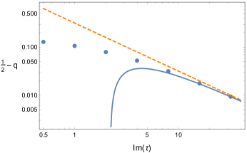
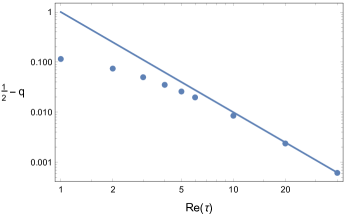
Figure 1: The points are numerically determined values for $q$ at different values of $\tau$ and with $n=1$. The straight lines are the nonzero leading order saddle point approximations for $\frac{1}{2}-q$ while the blue curve on the left is the second order correction. In the plot on the left $\operatorname{Re}\tau=0$ while in the plot on the right $\operatorname{Im}\tau=0$.

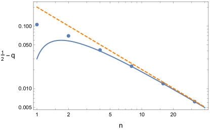
Figure 2: The points are numerically determined values for $q$ at various values of $n$ for $\tau=i$. The straight and curved lines are the first and second order saddle point approximations respectively for $\frac{1}{2}-q$ at large $n$.

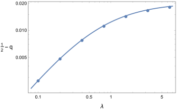
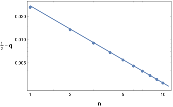
Figure 3: The points are numerically determined values for $q$ and the straight line is the first order saddle point approximation in the fixed $\lambda$, large $n$ limit for $\alpha=\frac{\pi}{2}$: (left) various values of $\lambda$ and $n=10$; (right) various values of $n$ and $\lambda=0.1$.

Large $\tau$

When $|\tau|$ is large, parametrizing $\tau=|\tau|e^{i\alpha}$, expanding to quartic order around the saddle point, we find $|Z|$ is minimized when

$$q_{f}=\frac{1}{2}-\frac{\sin\alpha}{\pi|\tau|}-\frac{\pi^{2}-4+(4+(1+2n)\pi^{2})\cos(2\alpha)}{4\pi^{2}|\tau|^{2}}+O(|\tau|^{-3})\ .$$ (83)

The decoupled case $\alpha=0$ matches the large Chern-Simons level calculation performed at the end of Jafferis:2010un . We have confirmed this formula for certain special cases ($\alpha=0$ and $\alpha=\pi/2$ with $n=1$) through numerical integration of (73) (see figure 1). At the critical point

$$|Z|^{2}=\frac{1}{2^{2n}|\tau|}-\frac{\pi n\sin\alpha}{2^{2n+1}|\tau|^{2}}+\frac{n(\pi^{2}n-8+(8-(2+3n)\pi^{2})\cos(2\alpha))}{2^{2n+4}|\tau|^{3}}+O(|\tau|^{-4})\ .$$ (84)

We can furthermore compute the two-point functions of the gauge and flavor currents. We leave it to the reader to apply the sum rule (81) and compute the two-point function of the topological current:

$$\Pi_{ff}=2n-\frac{n(\pi^{2}-8)\sin\alpha}{\pi|\tau|}+\frac{-2n(8+\pi^{2})+n(16+10\pi^{2}-(2+n)\pi^{4})\cos(2\alpha)}{2\pi^{2}|\tau|^{2}}+\mathcal{O}(|\tau|^{-3})\,,$$

$$\kappa_{ff}=\frac{n\pi^{2}\cos\alpha}{4|\tau|}-\frac{n\pi\Big{(}2\pi^{2}-8+8n+n\pi^{2}\Big{)}\sin 2\alpha}{8|\tau|^{2}}+\mathcal{O}(|\tau|^{-3})\,,$$ (85)

$$\Pi_{gg}=2n-\frac{n((n+1)\pi^{2}-8)\sin(\alpha)}{\pi|\tau|}+O(|\tau|^{-2})\ ,$$

$$\kappa_{gg}=\frac{\pi^{2}n(8n+(n+2)\pi^{2})\cos(\alpha)}{|\tau|}+O(|\tau|^{-2})\ .$$ (86)

Note that $\Pi_{ff}$ and $\Pi_{gg}$, which are proportional to conductivities, decrease as the coupling $1/\tau$ increases. This behavior is in accord with physical intuition, that increased scattering between quasi-particles in a weakly coupled description will hinder transport. The Hall conductivity which is proportional to $\kappa$, on the other hand, has a sign determined by the real part of $\tau$. These results are in principle accessible via perturbation theory. In practice, even the leading order term involves a sum over several one loop diagrams.

Large $n$

We can equivalently perform a saddle point integration in the limit of large $n$. In this case, we find instead

$$q_{f}=\frac{1}{2}-\frac{2}{\pi^{2}n}+\frac{2\left(12-\pi^{2}+2\pi\operatorname{Im}\tau\right)}{\pi^{4}n^{2}}+O(n^{-3})\ .$$ (87)

We confirmed this result numerically, for the special case $\tau=i$ (see figure 2). At the critical point,

$$|Z|^{2}=2^{-2n}\left(\frac{2}{\pi n}-\frac{8-\pi^{2}+4\pi\operatorname{Im}\tau}{\pi^{3}n^{2}}+O(n^{-3})\right)\ .$$ (88)

The associated current two-point functions are

$$\Pi_{ff} = 2n+\frac{2}{\pi^{2}}(16-\pi^{2})+\frac{2(-224+12\pi^{2}+\pi^{4}-2\pi(24-\pi^{2}))|\tau|\sin(\alpha)}{\pi^{4}n}+\mathcal{O}(n^{-2})\,,$$

$$\kappa_{ff} = -\frac{(16-\pi^{2})|\tau|\cos\alpha}{\pi^{2}n}+\mathcal{O}(n^{-2})\,,$$ (89)

$$\Sigma_{gg} = \tau+\frac{2\mathrm{i}\tau^{2}}{2n}+\frac{2(\pi^{2}-8)\mathrm{i}\tau^{2}-4\pi\tau^{3}}{\pi^{3}n^{2}}+O(n^{-3})\ .$$ (90)

Applying the sum rule (81) to these results, we find that $\Sigma_{tt}$ is $O(n^{-1})$.

Large $\tau$ and large $n$

In the case when $n$ and $|\tau|$ are both large, we can consider a perturbative expansion in $\frac{1}{n}$ keeping the ratio $\frac{n}{|\tau|}=\lambda$ fixed. In this case, the partition function extremizes for

$$q_{f}=\frac{1}{2}-\frac{2\lambda(\pi\lambda+2\sin\alpha)}{\pi(4+\pi^{2}\lambda^{2}+4\pi\lambda\sin\alpha)n}+\mathcal{O}(n^{-2})\,,$$ (91)

where $\tau=|\tau|e^{i\alpha}$. The agreement of this result with numerical evaluation of the partition function is remarkably good; see figure 3. The partition function for the above value of the R-charge and $\alpha=\frac{\pi}{2}$ is given by

$$|Z|^{2}=\frac{\lambda}{4^{n}n(2+\pi\lambda)}\Big{[}2+\frac{(-8+\pi^{2})\lambda^{2}}{n(2+\pi\lambda)^{2}}+\mathcal{O}(n^{-2})\Big{]}\,.$$ (92)

The flavor current two-point function in this limit is

$$\Pi_{ff} = 2n-\frac{2\lambda}{\pi(4+\pi^{2}\lambda^{2}+4\pi\lambda\sin\alpha)^{2}}\Big{(}\pi\lambda(-64+\pi^{4}\lambda^{2}+\pi^{2}(8-16\lambda^{2}))$$

$$+4\pi(16-\pi^{2})\lambda\cos 2\alpha+(-64+6\pi^{4}\lambda^{2}+8\pi^{2}(1-10\lambda^{2}))\sin\alpha\Big{)}+\mathcal{O}(n^{-1})\,.$$

$$\kappa_{ff} = \frac{\pi\lambda\cos\alpha\Big{[}\pi(4-(16-\pi^{2})\lambda^{2})-4(8-\pi^{2})\lambda\sin\alpha\Big{]}}{(4+\pi^{2}\lambda^{2}+4\pi\lambda\sin\alpha)^{2}}+\mathcal{O}(n^{-1})\,.$$ (93)

In particular, for $\alpha=\frac{\pi}{2}$, $\kappa$ must vanish by parity, and the above expression for $\Pi$ simplifies to

$$\Pi_{ff}=2n+\frac{2\lambda\Big{(}16-2\pi^{2}+\pi(16-\pi^{2})\lambda\Big{)}}{\pi(2+\pi\lambda)^{2}}+\mathcal{O}(n^{-1})\,,$$ (94)

The behavior of $\Pi_{ff}$ in the double scaling limit (93) is interesting; see figure 4. The result (93) reproduces (5.1) when $\lambda\to 0$ and (5.1) when $\lambda\to\infty$. For small $\lambda$, increasing the coupling $\lambda$ acts to decrease the transport coefficient $\Pi_{ff}$ as expected. However, as $\tau$ gets smaller, there is eventually an inversion and $\Pi_{ff}$ starts to get larger as the coupling increases. This type of behavior suggests that as $\lambda$ increases, there may at some point be a better weakly coupled description with a dual $\tau^{\prime}$. Increasing $|\tau^{\prime}|$ would correspond to decreasing $|\tau|$. Thus $\Pi$ again follows our intuition but with respect to the weakly coupled description. We shall return to this idea of a dual description in the next section.

The result for the gauge conductivity interpolates between the results (86) at small $\lambda$ and (90) and large $\lambda$:

$$\Pi_{gg} = \frac{4n(2+\pi\lambda\sin(\alpha))}{4+\pi^{2}\lambda^{2}+4\pi\lambda\sin(\alpha)}+O(n^{0})\ ,$$ (95)

$$\kappa_{gg} = \frac{\pi^{2}n\lambda\cos(\alpha)}{4+\pi^{2}\lambda^{2}+4\pi\lambda\sin(\alpha)}+O(n^{0})\ .$$ (96)

Already the first order term is nontrivial.

Figure 4: A plot of $\Delta\Pi=\Pi_{ff}-2n$ in the large $n$ and $\tau$ limit with $\lambda=n/|\tau|$ fixed. From top to bottom on the right, the curves correspond to $\alpha=0$, $\frac{\pi}{6}$, $\frac{\pi}{4}$, and $\frac{\pi}{2}$. The minimum at $\alpha=0$ occurs when $\lambda=\sqrt{\frac{2}{32-\pi^{2}}}$ and $\Delta\Pi=-\frac{\pi^{2}}{32}$. The minimum at $\alpha=\frac{\pi}{2}$ occurs at $(\lambda,\Delta\Pi)=\left(\frac{2\pi^{2}-16}{\pi(24-\pi^{2})},-\frac{(\pi^{2}-8)^{2}}{16\pi^{2}}\right)$.

5.2 Residue Method

For rational values of $\tau$, the integral (73) can be performed by contour integration. The central idea is to take advantage of a quasiperiodic property of the integrand for these special values. (Indeed, this same method can be employed to perform the usual Gaussian integral by contour integration Kneser ; Remmert .) Assume we have a definite integral

$$\int f(\sigma){\rm d}\sigma$$ (97)

and an extension of the integrand to the complex plane with the quasi-periodic property that $f(z+a)f(z-a)=f(z)^{2}$. Assume furthermore that $f(z)$ dies off suitably fast as $|{\rm Re}(z)|\to\infty$. Then one can replace the original integral with a contour integral

$$\int f(\sigma){\rm d}\sigma=\oint_{C}\frac{f(z)}{1-\frac{f(z)}{f(z-a)}}{\rm d}z$$ (98)

where the contour runs from $-\infty$ to $\infty$ on the real axis and then back from $+\infty$ to $-\infty$ along the line ${\rm Im}(z)={\rm Im}(a)$. The contour integral can be replaced in turn by a sum over poles inside the strip $0<{\rm Im}(z)<{\rm Im}(a)$.

In our case,

$$f(z)=e^{\mathrm{i}\pi\tau z^{2}+2\pi q_{t}z}\exp\left[n_{+}\ell(1-q_{+}+\mathrm{i}z)+n_{-}\ell(1-q_{-}-\mathrm{i}z)\right]$$ (99)

is quasiperiodic with respect to $a=is$ when $s^{2}\tau=r$ for $r$ and $s$ integers if $n_{+}+n_{-}$ is even. Otherwise, for $n_{+}+n_{-}$ odd, we have the restriction $s^{2}\left(\tau+\frac{1}{2}\right)=r$. Interestingly, for $s=1$, these cases correspond precisely to the decoupling limits, where the partition function is equal to that of a purely 3d Chern-Simons theory, with the appropriate Chern-Simons level, either integer or half-integer depending on the parity of $n_{+}-n_{-}$.

In general, the poles can be determined by solving for the roots of a polynomial. In the case $q_{+}=q_{-}=1/2$, the poles all lie on the imaginary axis and are easy to characterize. (See Appendix B for results pertaining to these cases.) For more general values of the R-charges, the poles move off, and the story gets rich, especially, since we are supposed to extremize with respect to $q_{+}$ and $q_{-}$. Our strategy will be to limit complexity by examining cases where finding the poles involves solving only a linear or quadratic equation. We will consider 1) $n_{+}=1$ and $n_{-}=0$; 2) $n_{+}=2$ and $n_{-}=0$; 3) $n_{+}=1$ and $n_{-}=1$; 4) $n_{+}=2$ and $n_{-}=2$. To simplify notation, we will present the results in terms of a single $q$ which is either $q_{f}$ in the cases $n_{+}=n_{-}$ or $q_{+}$ when $n_{-}=0$. We will largely ignore the dependence on $q_{g}$ and $q_{t}$. Note that as $\tau$ is real in this analysis, there is no distinction between $q_{g}$ and $q_{t}$ unles $\tau=0$.

The integral (73) appears also in studies of hyperbolic geometry and integrable systems. In ref.  Garoufalidis:2014ifa , using this contour integration method, the authors provide a residue formula for a generalization of (73). In our context, the interpretation would be a partition function of an abelian Chern-Simons theory on a squashed three sphere, for rational value of the squashing parameter. The sum over poles was then later cast as a sum over “Bethe roots”, thus making a connection with integrability Closset:2018ghr .

$n_{+}=1$ and $n_{-}=0$

To compute the partition function by our residue method, the poles correspond to roots of the following algebraic equation in $x=e^{2\pi\sigma}$:

$$x^{1+r}+xe^{\mathrm{i}\pi(r+q)}-e^{\mathrm{i}\pi(r-q)}=0\ ,$$ (100)

where we have set $\tau=r+\frac{1}{2}$.

This polynomial is already quite interesting from the point of view of hyperbolic geometry. The work Dimofte:2011ju proposed an interesting correspondence between supersymmetric gauge theories in three dimensions and the geometry of three manifolds. One example that they study closely, which forms in fact a building block to construct more complicated geometries and gauge theories, is the $n_{+}=1$ and $n_{-}=0$ theory with $\tau=\frac{1}{2}$.

We may consider the volumes of the three smallest hyperbolic three-manifolds. They can be computed in the following way. The volume is the imaginary part of an expression involving a dilogarithm:

$$\operatorname{Im}\left({\rm Li}_{2}(x)+\log|x|\log(1-x)\right)\ ,$$ (101)

and let $x$ be the root of (100) with a positive imaginary part. In particular, for the smallest manifold, also called the Weeks manifold, we take $r=2$ and $q=1$ for which we need a root of $x^{3}-x+1$. The volume is $0.942707$. For the second smallest manifold, sometimes called the Thurston manifold, $r=3$ and $q=1$, for which we need a root of $x^{4}+x-1$. The volume is $0.981369$. Finally, the third smallest manifold comes from $r=1$ and $q=0$ with polynomial $x^{2}-x+1$. Now the roots are cube roots of $-1$, and the volume is $1.01494$.

In fact, ref. Gang:2017lsr already pointed out this relation. They considered the partition function of this $n_{+}=1$ and $n_{-}=0$ theory on a warped $S^{3}$, in the limit where the $S^{3}$ approaches $S^{2}\times S^{1}$. They noticed that the saddle point evaluation of the log of the partition function gave precisely these three minimal volumes.

To keep our life simple we will consider only $\tau=\frac{1}{2}$ and $\tau=\frac{3}{2}$ so that we do not need to solve more than a quadratic equation. In the case $\tau=\frac{1}{2}$, the one pole is at

$$x_{0}=\frac{e^{-i\pi q}}{1+e^{i\pi q}}\ .$$ (102)

The branch cut of the log can be adjusted to put the imaginary part of $\sigma_{0}\equiv\frac{1}{2\pi}\log x_{0}$ between zero and one, leading to the residue formula for the partition function $Z[\tau,q]$:

$$Z\left[\frac{1}{2},q\right]=\frac{ie^{\frac{\mathrm{i}}{2}\pi\sigma_{0}^{2}}}{1+e^{\mathrm{i}\pi q}}\exp\left[\ell(1-q+i\sigma_{0})\right]\ .$$ (103)

We can use some dilogarithm identities to re-express this result in a simpler way:

$$Z\left[\frac{1}{2},q\right]=\exp\left[\ell\left(\frac{q+1}{2}\right)-\frac{\mathrm{i}\pi}{24}(3q-1)^{2}+\frac{\mathrm{i}\pi}{12}\right]\ .$$ (104)

We have recovered up to a phase the partition function of a single chiral field with R-charge $\frac{1-q}{2}$. The only critical points of this partition function in the allowed range $0<q<2$ are at $q=0$ and $q=2$. As $q=2$ leads to a chiral superfield with dimension below the unitarity bound, we take $q=0$ and find a free chiral with R-charge $1/2$. This result is in agreement with Intriligator:2013lca .

In the case $\tau=\frac{3}{2}$, we have two poles at

$$x_{\pm}=\frac{1}{2}\left(e^{\mathrm{i}\pi q}\pm e^{-\frac{\mathrm{i}}{2}\pi q}\sqrt{e^{3\mathrm{i}\pi q}-4}\right)\ .$$ (105)

Now the partition function becomes a sum over two terms

$$Z\left[\frac{3}{2},q\right] = \frac{1}{4\pi}\left(\left(1+\frac{e^{\mathrm{i}\pi q/2}}{\sqrt{e^{3\mathrm{i}\pi q}-4}}\right)e^{\frac{3}{2}\mathrm{i}\pi\sigma_{+}^{2}+\ell(1-q+i\sigma_{+})}+\right.$$ (106)

$$\left.\hskip 72.26999pt+\left(1-\frac{e^{\mathrm{i}\pi q/2}}{\sqrt{e^{3\mathrm{i}\pi q}-4}}\right)e^{\frac{3}{2}\mathrm{i}\pi\sigma_{-}^{2}+\ell(1-q+i\sigma_{-})}\right)$$

where $\sigma_{\pm}\equiv\frac{1}{2\pi}\log x_{\pm}$. Here the absolute value of the partition function is minimized at $q=\frac{1}{3}$. There is a local minimum as well, at $q=1.95185$. We do not have a good understanding why there are two minima in this case.

$n_{+}=2$ and $n_{-}=0$

As $n_{+}+n_{-}$ is even, we take instead $\tau=r$ to be an integer. The algebraic equation determining the location of the poles is

$$x^{1+r}e^{2\mathrm{i}\pi q}+x^{2}e^{\mathrm{i}\pi(4q+r)}-2xe^{\mathrm{i}\pi(2q+r)}+e^{\mathrm{i}\pi r}=0$$ (107)

Already when $\tau=0$, there are two poles:

$$x_{\pm}=\frac{1}{2}(1\pm i\sqrt{3})e^{-2\mathrm{i}\pi q}\$$ (108)

for which the partition function becomes a sum over two terms

$$Z\left[0,q\right]=\frac{1}{\sqrt{3}}\left(e^{2\ell(1-q+i\sigma_{+})}-e^{2\ell(1-q+i\sigma_{-})}\right)\ .$$ (109)

This expression has a vanishing derivative with respect to $q$ and can be simplified to give the following constant

$$Z\left[0,q\right]=\frac{2}{\sqrt{3}}\sinh\left[\frac{{\rm Li}_{2}(e^{\mathrm{i}\pi/3})-{\rm Li}_{2}(e^{-\mathrm{i}\pi/3})}{2\pi\mathrm{i}}\right]\approx 0.379568\ .$$ (110)

The argument of the hyperbolic sine function is the volume of an ideal tetrahedron in ${\mathbb{H}}^{3}$, $1.01494\ldots$, divided by $\pi$. The result (110) is a special case of the general integral formula proven in ref. Garoufalidis:2014ifa . The independence of the result with respect to $q$ follows from the possibility of changing the integration variable $\sigma\to\sigma-iq$ and then shifting the contour in (73), without crossing a pole.

We can analyze $\tau=1$, for which there are two poles as well, but we shall go no higher to avoid solving a cubic polynomial. In this case, the poles are at

$$x_{\pm}=\frac{e^{-\mathrm{i}\pi q}}{e^{\mathrm{i}\pi q}\pm 1}$$ (111)

and the partition function evaluates to

$$Z[1,q]=\frac{\mathrm{i}}{2}\left(\frac{e^{\mathrm{i}\pi\sigma_{+}^{2}+2\ell(1-q+i\sigma_{+}))}}{1+e^{\mathrm{i}\pi q}}+\frac{e^{\mathrm{i}\pi\sigma_{-}^{2}+2\ell(1-q+i\sigma_{-})}}{1-e^{\mathrm{i}\pi q}}\right)\ .$$ (112)

Through the use of dilogarithm identities, this expression can be massaged somewhat. Note the first term is close to the square of (103). The same sort of techniques that yield (104) from (103) can be used on the second term, and the end result is

$$Z[1,q]=\frac{1}{2}e^{-\frac{\mathrm{i}\pi}{12}(3q-2)^{2}+\frac{2\mathrm{i}\pi}{3}}\left(e^{2\ell\left(\frac{q}{2}\right)}-2\cos\left(\frac{\pi q}{2}\right)e^{2\ell\left(\frac{q+1}{2}\right)+\frac{\mathrm{i}\pi}{4}}\right)\ .$$ (113)

This partition function has minima at $q=0.231071$ and $q=1.44196$. If we allow the two chiral fields to have different R-charge, however, we find that in the full flavor space, $q=1.44196$ is a saddle point while $q=0.231071$ remains a minimum.

$n_{+}=1$ and $n_{-}=1$

For $\tau=r$ an integer, the locations of the poles are given by solutions of the polynomial equation

$$x^{1+r}-e^{2\mathrm{i}\pi q}x^{r}-e^{\mathrm{i}\pi(2q+r)}x+e^{\mathrm{i}\pi r}=0\ .$$ (114)

When $r=0$, there is a single pole at $z=\frac{\mathrm{i}}{2}$, and the partition function evaluates to

$$Z\left[0,q\right]=\frac{e^{2\ell\left(\frac{1}{2}-q\right)}}{2\sin(\pi q)}\ .$$ (115)

This case was analyzed already by ref.  Jafferis:2010un in the context of this model’s duality to the XYZ model – a theory with three hypermultiplets $X$, $Y$, and $Z$, a superpotential, and no gauge field. The relation can be made more explicit at the level of the partition function by employing a dilogarithm identity to rewrite the right hand side of (115) as $e^{2\ell(q)-\ell(2q-1)}$. Ref.  Jafferis:2010un also noted the extremum at $q=\frac{1}{3}$, in correspondence with the fact that the scalar $X$ field can be thought of as a composite of two fermions in the gauge theory. There are other special values of $q$. At $q=0$, 1, and 2, $\operatorname{Re}(\log Z)\to\infty$ while at $q=3/2$, $\operatorname{Re}(\log Z)\to-\infty$. The physical reasons behind these divergences remain obscure to us.

When $\tau=1$, there are poles at $z=\frac{\mathrm{i}}{2}$ and $z=0$. (The pole at $z=0$ can be swapped for one at $z=\mathrm{i}$.)

$$Z[1,q]=\frac{\cot(\pi q)-\mathrm{i}}{4}e^{2\ell(-q)}+\frac{1}{2}(-1)^{3/4}e^{-\mathrm{i}\pi q}e^{2\ell\left(\frac{1}{2}-q\right)}\ .$$ (116)

Numerically, this function has a minimum at $q=0.384466$. There is also a local minimum at $q=1.61553$. However, if we allow the charges to shift in opposite directions as well, $q_{+}=q+\delta q$ and $q_{-}=q-\delta q$, then we see that the critical point at $q=1.61553$ is only a saddle point while $q=0.384466$ remains a minimum.

$n_{+}=2$ and $n_{-}=2$

As the number of flavors increases, the polynomial determining the location of the poles becomes more complicated. In this case, we have

$$x^{r+2}-2e^{2\mathrm{i}\pi q}x^{1+r}+e^{4\mathrm{i}\pi q}x^{4}-e^{\mathrm{i}\pi(4q+r)}x^{2}+2e^{\mathrm{i}\pi(2q+r)}-e^{\mathrm{i}\pi r}=0$$ (117)

having set again $\tau=r$ to an integer. When $\tau=0$, there are two poles, one at $z=\frac{\mathrm{i}}{2}$ and then one that we may either take at $z=0$ or $z=\mathrm{i}$. The partition function is

$$Z[0,q]=\frac{e^{4\ell\left(-q\right)}}{32\sin^{3}(\pi q)\cos(\pi q)}-\frac{e^{4\ell\left(\frac{1}{2}-q\right)}}{4\sin(2\pi q)}\ .$$ (118)

There is an extremum at $q=0.408533$. There is also singular behavior, $\operatorname{Re}(\log Z)\to\infty$ at $q=0$, 1, 3/2, and 2, while at $q=1.187$ and 1.713, $\operatorname{Re}(\log Z)\to-\infty$.

6 S Duality and Transport

In this section, we investigate a strong-weak coupling duality $\tau\to-1/\tau$ that we implement at the level of our hemisphere partition function by Fourier transform. We will pay particular attention to two very simple theories, the $n_{+}=n_{-}=1$ theory and the $n_{+}=1$, $n_{-}=0$ theory. In both instances, we will be able to identify a particular value of $\tau$ where the theory becomes almost self-dual. Inspired by refs. Herzog:2007ij ; Hsiao:2017lch but with some crucial differences, we can use “self-duality” to extract the conductivity.

6.1 The $n_{+}=n_{-}=1$ theory

The trick to implementing the Fourier transform of the partition function is the residue method we described in the previous section. For the theory with $n_{+}=n_{-}=1$, the Fourier transform of interest is a generalization of the result (115) of the $\tau=0$ partition function:

$$\int{\rm d}\sigma e^{\ell(1-q_{+}+\mathrm{i}\sigma)+\ell(1-q_{-}-\mathrm{i}\sigma)+2\pi\mathrm{i}k\sigma}=e^{\ell(1-q_{+}-q_{-})+\ell(\frac{q_{+}+q_{-}}{2}+\mathrm{i}k)+\ell(\frac{q_{+}+q_{-}}{2}-\mathrm{i}k)+\pi k(q_{+}-q_{-})}\ .$$ (119)

Previously, we used the $k=0$, $q_{+}=q_{-}$ case of this integral to review the relation between the strong coupling limit of the $n_{+}=n_{-}=1$ theory and the XYZ Wess-Zumino model.

With this Fourier transform, we can perform an S duality on the partition function for the $n_{+}=n_{-}=1$ case with arbitrary $\tau$:

$$\int{\rm d}\sigma e^{\mathrm{i}\pi\tau\sigma^{2}+\ell(1-q_{f}-q_{g}+\mathrm{i}\sigma)+\ell(1-q_{f}+q_{g}-\mathrm{i}\sigma)+2\pi q_{t}\sigma}$$

$$= \frac{e^{\ell(1-2q_{f})}}{\sqrt{-\mathrm{i}\tau}}\int{\rm d}k\,e^{-\mathrm{i}\pi k^{2}/\tau+\ell(q_{f}+q_{t}+\mathrm{i}k)+\ell(q_{f}-q_{t}-\mathrm{i}k)+2\pi(k-\mathrm{i}q_{t})q_{g}}\ .$$

This S duality is a generalization to arbitrary coupling of the XYZ duality. The duality has swapped the role of the topological and the gauge symmetry; we can introduce primed quantities on the right hand side of the equality such that $q_{g}^{\prime}=-q_{t}$ and $q_{t}^{\prime}=q_{g}$. By symmetry, we expect the partition function to be minimized when $q_{t}=q_{g}=0$. From the presence of the $\ell(z)$ functions, we can read off that the new theory has two chiral multiplets of R-charge $1-q_{f}\pm q_{t}$ which couple to a U(1) gauge field with strength $-1/\tau$ and a third decoupled chiral with R-charge $2q_{f}$. The sum of the R-charges is two, commensurate with having a cubic superpotential linear in each of the three fields. In the limit $\tau\to 0$, we can evaluate the integral by saddle point, recovering (115). Indeed, one can analyze the system not only at the strong coupling fixed point but near it as well. Near the strong coupling fixed point, $|Z|$ is extremized when $q_{+}=q_{-}=q_{f}$ and

$$q_{f}=\frac{1}{3}+\frac{54\sqrt{3}-90\pi+8\sqrt{3}\pi^{2}}{9(8\pi(3\sqrt{3}-2\pi)-27)}\operatorname{Im}\tau+O(|\tau|^{2})\ .$$ (121)

We can also compute the current two point functions:

$$\Pi_{ff} = \Big{(}\frac{16}{3}-\frac{4\sqrt{3}}{\pi}\Big{)}+\frac{8(297-102\sqrt{3}\pi+32\pi^{2})}{27(3\sqrt{3}-4\pi)}\text{Im}\,\tau+\mathcal{O}(|\tau|^{2})\ ,$$

$$\kappa_{ff} = \frac{2\pi(27-18\sqrt{3}\pi+8\pi^{2})}{9(3\sqrt{3}-4\pi)}\text{Re}\,\tau+\mathcal{O}(|\tau|^{2})\ ,$$ (122)

$$\Pi_{gg} = \Pi^{\prime}_{tt}=\frac{4}{\pi}\text{Im}\,\tau+\frac{4(4\pi-3\sqrt{3})\cos(2\alpha)}{9\pi}|\tau|^{2}+O(|\tau|^{3})\ ,$$

$$\kappa_{gg} = \kappa^{\prime}_{tt}=\frac{8}{9}(3\sqrt{3}-2\pi)\pi^{2}\sin(2\alpha)|\tau|^{2}+O(|\tau|^{3})\ .$$ (123)

Numerically, the expansion for $\Pi_{ff}$ takes the form $3.13-2.32\,\text{Im}(\tau)+\ldots$. The 3.13 is larger than $\Pi_{ff}=2$ (5.1) we found in the free limit. The sign of the correction is what we anticipated in the discussion pertaining to figure 4. We have made manifest a “weakly coupled” description. Moving away from this description by increasing the gauge coupling initially tends to decrease the conductivity because of increased scattering. We put weakly coupled in scare quotes because the description is only weakly coupled vis a vis the 4d gauge field. There remain interactions governed by a superpotential between the three chiral fields.

The full behavior of $\Pi_{ff}$ and $\Pi_{gg}$ as a function of $\text{Im}\,\tau$ for $\text{Re}\,\tau=0$ can be seen in figure 5. While $\Pi_{ff}$ has a minimum, the gauged conductivity $\Pi_{gg}$ falls smoothly to zero as $\tau$ is decreased. The sum rule (81) gives us the behavior of the topological conductivity from $\Pi_{gg}$. In the strong coupling limit, we find that $\Pi_{tt}=\frac{1}{3}\Pi_{ff}$. Moving away from strong coupling, the topological conductivity decreases, eventually asymptoting to $\Pi_{tt}=\frac{4}{\pi\text{Im}\,\tau}$.

Something remarkable happens when $\tau=\mathrm{i}$ and $q_{+}=q_{-}=q_{f}=1/2$ (and $q_{g}=q_{t}=0$). The two partition functions on either side of (6.1) become manifestly equal, up to a factor of $e^{\ell(0)}/\sqrt{-\mathrm{i}\tau}$, which evaluates anyway to one. This equality points toward a self-duality of the underlying gauge theory. It is not in fact self-duality. Critically, the partition function is minimized not at $q_{f}=1/2$ but at $q_{f}=0.393814$. There is an additional neutral chiral multiplet in the dual frame that is not present in the original frame, and the charged chiral multiplets have different anomalous dimensions.

We can fix the issue about $q$ by taking advantage of the following dilogarithm identity:

$$e^{\ell(1-2q)}=e^{\ell(1/2-q)+\ell(1-q)-\ell(q-1/2)-\ell(q)}\ .$$ (124)

The duality statement can then be improved to

$$e^{\ell(q_{f}-1/2)+\ell(q_{f})}\int{\rm d}\sigma\,e^{\mathrm{i}\pi\tau\sigma^{2}+\ell(1-q_{f}-q_{g}+\mathrm{i}\sigma)+\ell(1-q_{f}+q_{g}-\mathrm{i}\sigma)+2\pi q_{t}\sigma}$$

$$= \frac{e^{\ell(1/2-q_{f})+\ell(1-q_{f})}}{\sqrt{-\mathrm{i}\tau}}\int{\rm d}k\,e^{-\mathrm{i}\pi k^{2}/\tau+\ell(q_{f}+q_{t}+\mathrm{i}k)+\ell(q_{f}-q_{t}-\mathrm{i}k)+2\pi q_{g}k-2\pi\mathrm{i}q_{t}q_{g}}\ .$$

Up to the factor $(-\mathrm{i}\tau)^{-1/2}$ suggesting the presence of a decoupled Maxwell field in the dual frame, the theory at coupling $\tau$ with R-charges parametrized by $q_{f}$ and $q_{g}$ has the same partition function as the theory at coupling $-1/\tau$ and R-charges parametrized by $q_{f}$ and $q_{t}$. By a parity argument, extremization will set $q_{t}=q_{g}=0$. Furthermore, now the partition function is minimized at $q_{f}=1/2$ when $\tau=\mathrm{i}$.

Let us say a little more about the field content of this modified theory and its dual. The original theory has neutral chirals $N_{1}$ and $N_{2}$ with R-charges $1/2-q_{f}$ and $1-q_{f}$ along with oppositely gauge charged chirals $C_{\pm}$ with R-charge $q_{f}\pm q_{g}$. The dual theory on the other hand has neutral chirals $\tilde{N}_{1}$ and $\tilde{N}_{2}$ with R-charges $1/2+q_{f}$ and $q_{f}$ and gauge charged chirals $\tilde{C}_{\pm}$ with R-charge $1-q_{f}\mp q_{t}$. Interestingly, the charges $1/2\pm q_{f}$ of the $N_{1}$ and $\tilde{N}_{1}$ are in conflict with the unitarity bound in one or the other duality frame almost everywhere. (Since these are gauge neutral operators, we expect their R-charges – and correspondingly their conformal dimensions – to be greater than or equal to one half.) The one exception is the self-dual point $q_{f}=1/2$, where we can divide both sides of the partition function by $e^{\ell(0)}$ and remove these problematic fields from the theory. Meanwhile, we can form gauge invariant mesonic operators $M=C_{+}C_{-}$ and $\tilde{M}=\tilde{C}_{+}\tilde{C}_{-}$ and a superpotential from $N_{2}^{2}M$ or $\tilde{N}_{2}^{2}\tilde{M}$, indicating the theory likely has interactions that are separate from those mediated by the bulk vector multiplet.

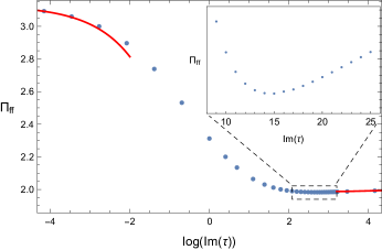
a) b)

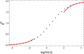
Figure 5: A plot of $\Pi$ vs. $\text{Im}\,\tau$ for the $n_{+}=n_{-}=1$ theory. We set $\text{Re}\,\tau=0$. The solid red curves are saddle point approximations, while the points are determined from numerical integration. a) The flavor symmetry. There is a minimum, visible in the inset, at $\tau\approx 15\mathrm{i}$. b) The gauge symmetry.

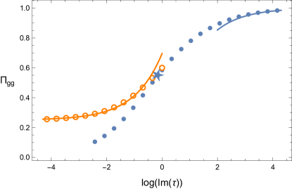
Figure 6: A plot of $\Pi_{gg}$ vs. $\text{Im}\,\tau$ for the $n_{+}=1$, $n_{-}=0$ theory. We set $\text{Re}\,\tau=0$. The solid points and the star have $\text{Re}\,\tau=0$ while the open orange circles have $\text{Re}\,\tau=1/2$. The star is the self-dual point. The curves are saddle point approximations.

Before moving on the to the $n_{+}=1$, $n_{-}=0$ theory, we note in passing that it is straightforward to generalize this S duality result to the case of $n$ flavors. We Fourier transform each pair of oppositely charged chirals independently, leading to a new theory with $n$ U(1) gauge fields. For simplicity, we give the result only in the case when $q_{i+}=q_{i-}=q_{i}$ where $i=1,\ldots,n$:

$$\int{\rm d}\sigma e^{\mathrm{i}\pi\tau\sigma^{2}+\sum_{i}\left(\ell(1-q_{i}+\mathrm{i}\sigma)+\ell(1-q_{i}-\mathrm{i}\sigma)\right)}$$

$$= \frac{1}{\sqrt{-\mathrm{i}\tau}}\int{\rm d}^{n}k\,e^{-\mathrm{i}\pi(\sum_{i}k_{i})^{2}/\tau+\sum_{i}\left(\ell(q_{i}+\mathrm{i}k_{i})+\ell(q_{i}-\mathrm{i}k_{i})+\ell(1-2q_{i})\right)}\ .$$

By Giveon-Kutasov duality Giveon:2008zn in the limit $\tau=k$ is an integer, the above result is also supposed to be the partition function of a $U(k+n-1)$ Chern-Simons theory at level $-k$. It would be interesting to check that (6.1) indeed matches the corresponding localization result for this non-abelian theory.

6.2 The $n_{+}=1$, $n_{-}=0$ theory

We can play a similar game with the theory of a single chiral multiplet, $n_{+}=1$ and $n_{-}=0$, and complexified gauge coupling $\tau$. By a change of variables $\sigma\to\sigma+2k$, we can deduce the Fourier transform of this single chiral theory from the partition function at $\tau=1/2$, (103):

$$\int{\rm d}\sigma e^{\mathrm{i}\pi\sigma^{2}/2+2\mathrm{i}\pi\sigma k+\ell(1-q_{g}+\mathrm{i}\sigma)}=e^{-2\mathrm{i}\pi k^{2}}e^{\ell(\frac{\tilde{q}+1}{2})-\frac{3\mathrm{i}\pi}{8}\left(\tilde{q}-\frac{1}{3}\right)^{2}+\frac{\mathrm{i}\pi}{12}}\ ,$$ (127)

where $\tilde{q}=q_{g}+2\mathrm{i}k$. This $q$ is most naturally identified with $q_{g}$ in the theories with $n_{+}=n_{-}$. Inserting this Fourier transform into the partition function at arbitrary $\tau$, we can perform an S duality and deduce the partition function for an associated theory with complexified gauge coupling $\tau^{\prime}=-(\tau-1/2)^{-1}-1/2$:

$$\int{\rm d}\sigma\,e^{\mathrm{i}\pi\tau\sigma^{2}+\ell(1-q_{g}+\mathrm{i}\sigma)+2\pi q_{t}\sigma}$$

$$= \frac{e^{-\frac{3\mathrm{i}\pi}{8}\left(q_{g}-\frac{1}{3}\right)^{2}+\frac{\mathrm{i}\pi}{2}q_{t}^{2}-\frac{3\mathrm{i}\pi}{2}\left(q_{g}-\frac{1}{3}\right)q_{t}+\frac{\mathrm{i}\pi}{12}}}{\sqrt{-\mathrm{i}(\tau-1/2)}}\int{\rm d}k\,e^{\mathrm{i}\pi\tau^{\prime}k^{2}+\ell\left(\frac{q_{g}+1}{2}+q_{t}+\mathrm{i}k\right)+2\pi\left(\frac{3q_{g}-1}{4}-\frac{q_{t}}{2}\right)k}\ .$$

This partition function is that of a single chiral with R-charge $\frac{1-q_{g}}{2}-q_{t}$. There is also a term in the exponent proportional to $2\pi\left(\frac{3q_{g}-1}{4}-\frac{q_{t}}{2}\right)k$, which corresponds to a monopole operator of dimension $(3q_{g}-1)/4-q_{t}/2$ Jafferis:2010un .

We can use a saddle point approximation to compute the R-charge near $\tau=\frac{1}{2}$. The calculation is more subtle than before because $q_{t}$ is nonzero near $\tau=\frac{1}{2}$. We find that

$$q_{g} = \frac{1}{4}+O(|\tau^{\prime}|^{-1})\ ,\;\;\;q_{g}+2q_{t}=\frac{2\sin(\alpha^{\prime})}{\pi|\tau^{\prime}|}+O(|\tau^{\prime}|^{-2})\ ,$$ (129)

where $\tau^{\prime}=|\tau^{\prime}|e^{\mathrm{i}\alpha^{\prime}}$. The combination $q_{g}+2q_{t}$ appears because in the limit $\tau\to 1/2$ where the complexified combination $q_{t}+\tau q$ becomes real and the two charges can no longer be distinguished, as was discussed above. The saddle point approximation also gives the two-point function of the symmetry current in this limit:

$$\Pi_{gg}=\frac{1}{4}+\frac{\left(\frac{52}{\pi}-3\pi\right)\sin(\alpha^{\prime})-12\cos(\alpha^{\prime})}{16|\tau^{\prime}|}+O(|\tau^{\prime}|^{-2}\ ,$$

$$\kappa_{gg}=\frac{3}{8}+\frac{3((\pi^{2}-12)\cos(\alpha^{\prime})-4\pi\sin(\alpha^{\prime}))}{64|\tau^{\prime}|}+O(|\tau^{\prime}|^{-2})\ .$$ (130)

We did not analyze this model via saddle point in the weak coupling $\tau\to\infty$ limit before, but let us do so here. The weak coupling limit is

$$q_{g} = \frac{1}{2}-\frac{\sin(\alpha)}{\pi|\tau|}-\frac{\pi^{2}-4+2(\pi^{2}+2)\cos(2\alpha)}{4\pi^{2}|\tau|^{2}}+{\mathcal{O}}(|\tau|^{-3})\ ,$$

$$q_{t} = -\frac{\cos(\alpha)}{4|\tau|}+O(|\tau|^{-2})\ ,$$

$$\Pi_{gg} = 1-\frac{3\pi^{2}-16}{4\pi|\tau|}\sin(\alpha)+{\mathcal{O}}(|\tau|^{-2})\ ,$$

$$\kappa_{gg} = \frac{3\pi^{2}\cos(\alpha)}{16|\tau|}+{\mathcal{O}}(|\tau|^{-2})\ .$$ (131)

The characteristics of $\Pi_{gg}$ as a function of $\tau$ are similar to what we found for $\Pi_{gg}$ for the $n_{+}=n_{-}=1$ theory. As we increase the coupling or equivalently decrease $\tau$, $\Pi_{gg}$ decreases because of the increased scattering. We have plotted $\Pi_{gg}$ vs. $\tau$ in figure 6, demonstrating that the saddle point approximations work reasonably well.

Something remarkable happens when $\tau$ takes its fixed point value $\mathrm{i}\sqrt{3}/2$ under the TST transformation $-(\tau-1/2)^{-1/2}-1/2$. The extremal value of the R-charge is $q=1/3$. At this point, $e^{\mathrm{i}\pi/12}$ in the numerator cancels against the $\sqrt{-\mathrm{i}(\tau-1/2)}$ in the denominator, and the two sides of (6.2) become manifestly equal. We view this equality as evidence for an underlying self-duality of the physical theory. Unlike the $n_{+}=n_{-}=1$ case, we have no need to invoke dilogarithm identities or modify the original setup.

6.3 Transport

The conductivities of both the modified $n_{+}=n_{-}=1$ theory and the $n_{+}=1$, $n_{-}=0$ theory take a particularly simple form at the self-dual point, namely

$$\Sigma_{gg}=\frac{\tau}{2}\ .$$ (132)

We would like to try to explain this fact by digging a little deeper into the field theory relations suggested by the integral equalities (6.1) and (6.2). In both cases, we can identify a doublet of transformed charges $(q^{\prime}_{g},q^{\prime}_{t})$ which are related to the original charges $(q_{g},q_{t})$ by a certain affine transformation. In the $n_{+}=n_{-}=1$ case, $q_{g}^{\prime}=-q_{t}$ and $q_{t}^{\prime}=q_{g}$, while for the $n_{+}=1$, $n_{-}=0$ case we find the more involved $q_{g}^{\prime}=\frac{1}{2}-\frac{1}{2}q_{g}-q_{t}$ and $q_{t}^{\prime}=-\frac{1}{4}+\frac{3}{4}q_{g}-\frac{1}{2}q_{t}$. From the discussion around the definition of the current-current two-point functions (77), it is clear that single derivatives of the partition function with respect to $q_{t}$ and $q_{g}$ are related to the associated currents $J_{t}$ and $J_{g}$, from which we may deduce the following transformation rule on the doublet

$$\left(\begin{array}[]{c}J_{g}^{\prime}\\ J_{t}^{\prime}\end{array}\right)=\left(\begin{array}[]{cc}a&b\\ c&d\end{array}\right)\left(\begin{array}[]{c}J_{g}\\ J_{t}\end{array}\right)$$ (133)

implied by the integral relations (6.1) and (6.2). The element of $SL(2,{\mathbb{R}})$ involved is the same one that transforms $\tau$ to the $\tau^{\prime}$ of the dual theory.

This transformation rule (133) implies a corresponding rule on the coefficients $\Sigma_{gg}$, $\Sigma_{gt}$, and $\Sigma_{tt}$ of the current two-point functions. This rule can then be substantially simplified with the help of the sum rules (81), yielding for $\Sigma_{gg}$ the constraint

$$\Sigma^{\prime}_{gg}=\left(a^{2}+\frac{2ab}{\tau}+\frac{b^{2}}{\tau^{2}}\right)\Sigma_{gg}-\frac{b^{2}}{\tau}\ .$$ (134)

Now we impose self-duality. Staring at the integral relations (6.1) and (6.2), the claim is that $\Sigma^{\prime}$ should be equal to $\Sigma$ up to the effect of the phases that have the schematic form

$$e^{\mathrm{i}\pi A(q_{g}-q_{0g})^{2}+\mathrm{i}\pi B(q_{t}-q_{t0})^{2}+\mathrm{i}\pi C(q_{t}-q_{t0})(q_{g}-q_{g0})}$$ (135)

where $A$, $B$, and $C$ are real constants and $q_{0g}$ and $q_{0t}$ are the critical values of $q_{g}$ and $q_{t}$ at self-duality. In the particular case of $\Sigma_{gg}$, we find then that

$$\Sigma_{gg}-A=\left(a^{2}+\frac{2ab}{\tau}+\frac{b^{2}}{\tau^{2}}\right)\Sigma_{gg}-\frac{b^{2}}{\tau}\ .$$ (136)

For the $n_{+}=n_{-}=1$ theory, $A=0$, $a=0$ and $b=-1$. For the $n_{+}=1$, $n_{-}=0$ theory, $A=-\frac{3}{8}$, $a=-\frac{1}{2}$, and $b=-\frac{3}{4}$. In both cases, one finds (132).

This self-duality, with its additional phases (135), is more delicate than what is usually discussed. The idea of a complexified conductivity transforming under $SL(2,{\mathbb{Z}})$ has a long history in the condensed matter literature, going back at least to Lutken:1991jk . In Witten’s Witten:2003ya large $n$ set up for instance, $\tau$ and $\Sigma_{gg}$ transform in precisely the same way under $SL(2,{\mathbb{Z}})$, suggesting that at a self-dual fixed point, $\Sigma_{gg}$ should be equal to $\tau$, not $\tau/2$.

Unlike graphene, our theory has an exact 2+1 dimensional Lorentz invariance where both the photon and electron travel at the same speed. In this context, refs. Hartnoll:2007ip ; Herzog:2009xv pointed out that Ward identities relate other transport coefficients to the conductivity. In particular, given the conductivity, one can also compute the thermoelectric coefficient and the heat conductivity. The arguments of refs. Hartnoll:2007ip ; Herzog:2009xv should be revisited in the present case, as they rely on having a 2+1 dimensional rather than a 3+1 dimensional stress tensor. We are optimistic that the conclusions are unchanged. In a nonsupersymmetric version of our theory, refs. Hsiao:2017lch ; Hsiao:2018fsc in fact use self-duality to compute these coefficients directly.

In standard discussions of self-duality, there is an interesting generalization to nonzero temperature and oscillating electric fields. In general, the optical conductivity may depend on a function of $\omega/T$ where $\omega$ is the frequency of the applied electric field Damle:1997rxu . Self-duality is supposed to constrain the conductivity to be independent of $\omega$ Herzog:2007ij . It would be interesting to explore if those arguments apply to the present case.

Finally, one can explore the consequences at nonzero charge density and magnetic field, which are relevant for quantum Hall physics. The boundary condition on the field strength relates the charge density $\rho$ to the boundary value of the electric field normal to the surface, and S duality will swap this electric field with the magnetic field $B$. Refs. Hsiao:2017lch ; Hsiao:2018fsc already exploited this feature to draw some conclusions about the quantum Hall effect at 1/2 filling in the nonsupersymmetric context. For carefully chosen values of $\rho$ and $B$, the theory will be invariant under S duality up to a relative change in sign between $\rho$ and $B$ which may in turn send $\sigma_{H}\to-\sigma_{H}$ if $\alpha=\pi/2$. With this constraint, one can fix $\sigma$ and $\sigma_{H}$. We will leave a more detailed investigation of these and other transport issues to future work.

7 Discussion

We had initially three different motivations for this project: understanding quantities that decrease under renormalization group flow in quantum field theory; the possibility of spontaneous flavor symmetry breaking in three dimensional QED; and boundary conditions in maximally supersymmetric Yang-Mills theory in four dimensions. While we laid some groundwork in each of these three directions, the main progress came from an unexpected direction – transport and duality. We were able to calculate conductivities at all values of the coupling in our theories. Furthermore, a pair of our theories turned out to be self-dual.

In conclusion, however, let us return to the original motivation. The best known example of a quantity that decreases under renormalization group flow is the $a$-anomaly. In conformal field theory, scale invariance implies that the trace of the stress tensor vanishes classically, $T^{\mu}_{\;\mu}=0$. However, quantum effects on a curved manifold lead to anomalous contributions which are proportional to curvature invariants. The $a$-anomaly, present in even dimensional cases, is the coefficient of the Euler density term, $T^{\mu}_{\;\mu}=aE_{d}+\ldots$, where the ellipses denote other possible curvature invariants. Regarding conformal field theories as fixed points in the renormalization group flow, it is proven that $a_{\rm UV}>a_{\rm IR}$ in $d=2$ and 4 Zamolodchikov:1986gt ; Komargodski:2011vj . The $a$-anomaly can also be defined using the sphere partition function; in particular, in even dimensions, there is an anomalous contribution $\log Z=2a\log\Lambda+\ldots$ where $\Lambda$ is an energy cut-off. While $\log Z$ is finite in odd dimensions, this relation to sphere partition functions suggests that more generally there may be a special role for $\log Z$ as a renormalization group monotone. Indeed, in three dimensions, it is also proven using entanglement entropy techniques that $F=-\log Z$ decreases under renormalization group flow Casini:2012ei .

Of course, our example is not a sphere but a hemisphere. The candidate renormalization group monotone for the four dimensional hemisphere is $F_{\partial}$ (74) Gaiotto:2014gha . As we discussed, up to some $\tau$ and $\overline{\tau}$ dependence that can be fixed by considering the free limit, our $\log Z$ is closely related to $F_{\partial}$.

A nice feature of these renormalization group monotones is that they are independent of certain marginal couplings. The quantity $a$ is independent because of Wess-Zumino consistency Wess:1971yu ; Osborn:1991gm . Ref. Gerchkovitz:2014gta used conformal symmetry to show $F$ is independent as well. However, there is a loophole concerning $F_{\partial}$, as one of us showed in ref. Herzog:2019rke ; Bianchi:2019umv . While $F_{\partial}$ is not expected to depend on boundary marginal deformations, it can depend on bulk ones. A motivation of this work was to explore precisely how $F_{\partial}$, or equivalently $Z_{HS^{4}}$, can depend on a bulk marginal parameter, namely $\tau$.

Looking to the future, there are two anomalous contributions to the stress tensor trace which are associated purely with the boundary, one proportional to the extrinsic curvature cubed and one proportional to a product of the extrinsic curvature and the Weyl curvature Herzog:2015ioa . It would be interesting to see whether these contributions can be isolated by generalizing our result to the case of a squashed hemisphere. The localization result for squashed three and four spheres is already known Hama:2012bg ; Hama:2011ea .

Regarding spontaneous symmetry breaking, an interesting idea put forward already in early work Gorbar:2001qt on these graphene-like theories, is that, at least in the non-supersymmetric case with $n$ Dirac boundary fermions, for large enough $g$, the global flavor symmetry may spontaneously break $U(2n)\to U(n)\times U(n)$ and a mass gap for the fermions appear. Part of the motivation of this work was to see if the behavior of the partition function makes such an effect visible in a supersymmetric example. The short answer is no, but let us follow this train of thought a little further.

A similar spontaneous breaking of flavor symmetry may also play a role in three dimensional QED Pisarski:1984dj ; Appelquist:1986fd . While the gauge coupling becomes large at low energy, there is a “line” of fixed points associated with the number $n$ of fermions. It is conjectured that below a critical value of $n$, this purely three dimensional theory may also generate a mass gap. The similarity between the graphene-like theory and ordinary three dimensional QED is no accident Kotikov:2016yrn . Perturbatively in $g$ and at large $n$, the Feynman rules of one theory can be mapped onto the other with the substitution $g^{2}\sim 1/n$. This map means that establishing a critical value for $g$ in our theory may shed light on the critical $n$ in three dimensional QED.

One might hope to investigate spontaneous symmetry breaking by looking at R-charge assignments. The R-charges obtained from the partition function can be used to establish the scaling dimensions of certain protected operators. If any of these operators fall below the unitarity bound, the theory may become unstable although the picture here is not crystal clear. In the context of renormalization group flows, these operators can also decouple and become free with limited effects on the rest of the theory. Decoupling has been observed in 4d and 3d supersymmetric gauge theory examples Safdi:2012re ; Agarwal:2012wd ; Morita:2011cs ; Kutasov:2003iy ; Barnes:2004jj . R-charge assignments thus provide a suggestive if not conclusive way of looking at the stability of the theory.

In our case, candidate theories to look into these effects are those with the smallest number of flavors, i.e. the $n_{+}=n_{-}=1$ and $n_{+}=1$, $n_{-}=0$ theories, in the limit $\operatorname{Im}(\tau)\to 0$. We found no evidence in either case to suggest an instability. As is well known, the $n_{+}=n_{-}=1$ theory is dual to the XYZ model as $\tau\to 0$, and this model is expected to be well behaved.

Interestingly, our self-dual modification to the $n_{+}=n_{-}=1$ theory did have unitarity bound issues. The necessity to add neutral scalars $N_{1}$ and $\tilde{N}_{1}$ with R-charges $1/2\mp q$ meant the theory could only be defined at the self-dual point where these scalars could be removed. Indeed, there is a conflict in defining a weakly coupled theory with a weak-strong duality that is unstable at strong coupling. The weak-strong coupling duality implies then that the theory is also unstable at weak coupling, that it may in fact only be defined at order one values of the coupling. Our modified $n_{+}=n_{-}=1$ theory resolves this issue by isolating itself and having a good unitary definition only at the self dual point, $\tau=\mathrm{i}$.

The $n_{+}=1$, $n_{-}=0$ theory was dual to a free chiral multiplet at $\tau=1/2$. While $\tau=1/2$ is well defined, we have a lingering suspicion that there may be issues for this theory for $\tau\neq 1/2$ but close to the real line. We were able to explore the theory near $\tau=1/2$ using the saddle point approximation but saw no smoking gun for an instability. We also found that the $n_{+}=1$, $n_{-}=0$ theory had a self-dual point at $\tau=\mathrm{i}\sqrt{3}/2$. Despite not seeing evidence for instabilities in this theory or the unmodified $n_{+}=n_{-}=1$ theory, these examples with small numbers of flavors have a number of interesting features which are worth further exploring.

A useful tool in the decoupling limit is the Witten index for supersymmetric Abelian Chern-Simons theory. Using the results of Intriligator:2013lca , the Witten index is always greater than or equal to zero for our Abelian theories, forbidding the breaking of supersymmetry, and presumably also flavor symmetry, at least in the decoupling limits.

The third motivation was the hope that the work here lays the groundwork for performing a similar localization calculation of ${\mathcal{N}}=4$ super Yang-Mills on $HS^{4}$, coupled to charged matter on the boundary. Much is known about supersymmetry preserving boundary conditions in ${\mathcal{N}}=4$ SYM Gaiotto:2008sa . Like the U(1) theory considered here, ${\mathcal{N}}=4$ super Yang-Mills with a boundary is an example of a boundary conformal field theory with an exactly marginal coupling – again the complexified gauge coupling $\tau$.

Finally, we mention in passing that the data we obtain here may be useful in applying the bootstrap program to boundary CFT. In particular, we may be able to constrain a bootstrap of this graphene-like theory or even 3d QED Chester:2016wrc .

Appendix A Fermion Conventions

The Clifford algebra in Euclidean signature comes from quotienting the free algebra associated to the gamma matrices by the relation

$$\{\gamma^{a},\gamma^{b}\}=2\delta^{ab}\ .$$ (137)

Our gamma matrices are Hermitian $(\gamma^{a})^{\dagger}=\gamma^{a}$. Our basis is the same that Narain et al. Gava:2016oep use

$$\gamma^{a}=\left(\begin{array}[]{cc}0&-\mathrm{i}\sigma^{a}\\ \mathrm{i}\sigma^{a}&0\end{array}\right)\ ;\;\;\;\gamma^{4}=\left(\begin{array}[]{cc}0&1\\ 1&0\end{array}\right)\ ,\;\;\;\gamma^{5}=\gamma^{1}\gamma^{2}\gamma^{3}\gamma^{4}=\left(\begin{array}[]{cc}1&0\\ 0&-1\end{array}\right)\ .$$ (138)

We can define two candidate charge conjugation matrices $C=\gamma_{1}\gamma_{3}={\rm diag}(-\mathrm{i}\sigma_{2},-\mathrm{i}\sigma_{2})$ and $\tilde{C}=\gamma_{2}\gamma_{4}\gamma_{5}={\rm diag}(-\mathrm{i}\sigma_{2},\mathrm{i}\sigma_{2})$. They are both incompatible with a Majorana condition since $C^{*}C=\tilde{C}^{*}\tilde{C}=-1$ but compatible with a symplectic Majorana condition. We choose $C$ to define symplectic Majorana fermions

$$\overline{\psi}_{i}\equiv(\psi_{i})^{\dagger}=\epsilon_{ij}(\psi^{j})^{T}C\ .$$ (139)

In particular, $\psi_{1}^{\dagger}=\psi^{2T}C$ and $\psi_{2}^{\dagger}=-\psi^{1T}C$. Furthermore, $\psi^{2}=C\psi_{1}^{*}$. The matrix $C$ satisfies the further conjugation properties

$$\gamma_{a}^{*}=\gamma_{a}^{T}=C\gamma_{a}C^{-1}\ ,\;\;\;C^{\dagger}=C^{T}=C^{-1}=-C\ ,\;\;\;C^{*}=C\ .$$ (140)

A.1 Curved Space

In curved space, we define vielbeins ${e^{a}}_{\mu}$ such that the combination $\delta_{ab}{e^{a}}_{\mu}{e^{b}}_{\nu}=g_{\mu\nu}$ yields the metric. The curved space gamma matrices are then

$$\gamma^{\mu}={e_{a}}^{\mu}\gamma^{a}\ ,$$ (141)

such that

$$\{\gamma^{\mu},\gamma^{\nu}\}=2g^{\mu\nu}\ .$$ (142)

The covariant derivative on the fermion is

$${\rm D}_{\mu}\psi=\partial_{\mu}\psi-\frac{\mathrm{i}}{4}\omega_{ab\mu}\sigma^{ab}\psi\ ,$$ (143)

where $\sigma^{ab}$ is a generator of the local Lorentz group in the spinor representation:

$$\sigma^{ab}=\frac{\mathrm{i}}{2}[\gamma^{a},\gamma^{b}]=\mathrm{i}\gamma^{ab}\ .$$ (144)

Appendix B Special Cases of the Localization Integral

For the special case $n=1$ and $q=1/2$, we find the following results, that depend on the parity of $r$ and $s$.

$r$ and $s$ both odd or both even:

$$\int\frac{e^{\mathrm{i}\pi\frac{r}{s^{2}}\sigma^{2}}}{2\cosh(\pi\sigma)}{\rm d}\sigma=\frac{\mathrm{i}s}{2r}\sum_{n=0}^{r-1}\frac{e^{-\frac{\mathrm{i}\pi n^{2}}{r}}}{\cos\left(\frac{\pi ns}{r}\right)}-\frac{\mathrm{i}}{2}\sum_{m=0}^{s-1}\frac{(-1)^{m}e^{-\frac{\mathrm{i}\pi r}{s^{2}}\left(m+\frac{1}{2}\right)\left(m+\frac{1}{2}-s\right)}}{\sin\left(\frac{\pi r\left(m+\frac{1}{2}\right)}{s}\right)}\$$ (145)

$r$ odd/even and $s$ even/odd:

$$\int\frac{e^{\mathrm{i}\pi\frac{r}{s^{2}}\sigma^{2}}}{2\cosh(\pi\sigma)}{\rm d}\sigma=\frac{\mathrm{i}s}{2r}\sum_{n=0}^{r-1}\frac{e^{-\frac{\mathrm{i}\pi\left(n+\frac{1}{2}\right)^{2}}{r}}}{\cos\left(\frac{\pi\left(n+\frac{1}{2}\right)s}{r}\right)}+\frac{1}{2}\sum_{m=0}^{s-1}\frac{(-1)^{m}e^{-\frac{\mathrm{i}\pi r}{s^{2}}\left(m+\frac{1}{2}\right)\left(m+\frac{1}{2}-s\right)}}{\cos\left(\frac{\pi r\left(m+\frac{1}{2}\right)}{s}\right)}\$$ (146)

Duality results when $q=1/2$:

$$\int\frac{e^{\mathrm{i}\pi\tau x^{2}}}{\cosh(\pi x)}{\rm d}x=\frac{1}{\sqrt{-i\tau}}\int\frac{e^{-\mathrm{i}\pi x^{2}/\tau}}{\cosh(\pi x)}{\rm d}x\ ,$$ (147)

$$\sqrt{-\mathrm{i}\tau}\int\frac{e^{\mathrm{i}\pi\tau x^{2}}}{\cosh(\pi x)^{n}}{\rm d}x=\int\frac{e^{-\mathrm{i}(\sum_{i}x_{i})^{2}/\tau}}{\prod_{i=1}^{n}\cosh(\pi x_{i})}{\rm d}^{n}x\ ,$$ (148)

$$\int\frac{{\rm d}x}{\cosh(\pi x)^{n}}=\frac{\Gamma\left(\frac{n}{2}\right)}{\sqrt{\pi}\Gamma\left(\frac{1+n}{2}\right)}\ .$$ (149)

References

- (1) E. V. Gorbar, V. P. Gusynin and V. A. Miransky, Dynamical chiral symmetry breaking on a brane in reduced QED, Phys. Rev. D64 (2001) 105028 [hep-ph/0105059].
- (2) S.-J. Rey, “Quantum phase transitions from string theory.”
- (3) D. B. Kaplan, J.-W. Lee, D. T. Son and M. A. Stephanov, Conformality Lost, Phys. Rev. D80 (2009) 125005 [0905.4752].
- (4) G. Grignani and G. W. Semenoff, Defect QED: Dielectric without a Dielectric, Monopole without a Monopole, 1909.03279.
- (5) W.-H. Hsiao and D. T. Son, Self-Dual Bosonic Quantum Hall State in Mixed Dimensional QED, 1809.06886.
- (6) W.-H. Hsiao and D. T. Son, Duality and universal transport in mixed-dimension electrodynamics, Phys. Rev. B96 (2017) 075127 [1705.01102].
- (7) S. Teber, Field theoretic study of electron-electron interaction effects in Dirac liquids, habilitation, Paris, LPTHE, 2017. 1810.08428.
- (8) L. Di Pietro, D. Gaiotto, E. Lauria and J. Wu, 3d Abelian Gauge Theories at the Boundary, JHEP 05 (2019) 091 [1902.09567].
- (9) C. P. Herzog and K.-W. Huang, Boundary Conformal Field Theory and a Boundary Central Charge, JHEP 10 (2017) 189 [1707.06224].
- (10) C. P. Herzog, K.-W. Huang, I. Shamir and J. Virrueta, Superconformal Models for Graphene and Boundary Central Charges, JHEP 09 (2018) 161 [1807.01700].
- (11) V. Pestun, Localization of gauge theory on a four-sphere and supersymmetric Wilson loops, Commun. Math. Phys. 313 (2012) 71 [0712.2824].
- (12) N. Hama and K. Hosomichi, Seiberg-Witten Theories on Ellipsoids, JHEP 09 (2012) 033 [1206.6359].
- (13) N. Hama, K. Hosomichi and S. Lee, SUSY Gauge Theories on Squashed Three-Spheres, JHEP 05 (2011) 014 [1102.4716].
- (14) N. Hama, K. Hosomichi and S. Lee, Notes on SUSY Gauge Theories on Three-Sphere, JHEP 03 (2011) 127 [1012.3512].
- (15) A. Kapustin, B. Willett and I. Yaakov, Exact Results for Wilson Loops in Superconformal Chern-Simons Theories with Matter, JHEP 03 (2010) 089 [0909.4559].
- (16) E. Gava, K. S. Narain, M. N. Muteeb and V. I. Giraldo-Rivera, gauge theories on the hemisphere , Nucl. Phys. B920 (2017) 256 [1611.04804].
- (17) M. Dedushenko, Gluing I: Integrals and Symmetries, 1807.04274.
- (18) M. Dedushenko, Gluing II: Boundary Localization and Gluing Formulas, 1807.04278.
- (19) D. Dudal, A. J. Mizher and P. Pais, Exact quantum scale invariance of three-dimensional reduced QED theories, Phys. Rev. D99 (2019) 045017 [1808.04709].
- (20) D. L. Jafferis, The Exact Superconformal R-Symmetry Extremizes Z, JHEP 05 (2012) 159 [1012.3210].
- (21) C. Closset, T. T. Dumitrescu, G. Festuccia, Z. Komargodski and N. Seiberg, Contact Terms, Unitarity, and F-Maximization in Three-Dimensional Superconformal Theories, JHEP 10 (2012) 053 [1205.4142].
- (22) S. Garoufalidis and R. Kashaev, Evaluation of state integrals at rational points, Commun. Num. Theor. Phys. 09 (2015) 549 [1411.6062].
- (23) M. P. A. Fisher, G. Grinstein and S. M. Girvin, Presence of quantum diffusion in two dimensions: Universal resistance at the superconductor-insulator transition, Phys. Rev. Lett. 64 (1990) 587.
- (24) X. G. Wen and A. Zee, Universal Conductance at the Superconductor - Insulator Transition, Int. J. Mod. Phys. B4 (1990) 437.
- (25) L. W. Engel, D. Shahar, C. Kurdak and D. C. Tsui, Microwave frequency dependence of integer quantum Hall effect: Evidence for finite-frequency scaling, Phys. Rev. Lett. 71 (1993) 2638.
- (26) D. Shahar, D. C. Tsui, M. Shayegan, E. Shimshoni and S. L. Sondhi, A Different View of the Quantum Hall Plateau-to-Plateau Transitions, Phys. Rev. Lett. 79 (1997) 479 [cond-mat/9611011].
- (27) I. Jeon and S. Murthy, Twisting and localization in supergravity: equivariant cohomology of BPS black holes, JHEP 03 (2019) 140 [1806.04479].
- (28) S. S. Pufu, The F-Theorem and F-Maximization, J. Phys. A50 (2017) 443008 [1608.02960].
- (29) D. Gaiotto, Boundary F-maximization, 1403.8052.
- (30) Z. Komargodski and A. Schwimmer, On Renormalization Group Flows in Four Dimensions, JHEP 12 (2011) 099 [1107.3987].
- (31) G. Gur-Ari, S. A. Hartnoll and R. Mahajan, Transport in Chern-Simons-Matter Theories, JHEP 07 (2016) 090 [1605.01122].
- (32) O. Aharony, G. Gur-Ari and R. Yacoby, Correlation Functions of Large N Chern-Simons-Matter Theories and Bosonization in Three Dimensions, JHEP 12 (2012) 028 [1207.4593].
- (33) G. Gur-Ari and R. Yacoby, Correlators of Large N Fermionic Chern-Simons Vector Models, JHEP 02 (2013) 150 [1211.1866].
- (34) H. Kneser, Funktionentheorie. Vandenhoeck and Ruprecht, 1958.
- (35) R. Remmert, Theory of Complex Functions. Springer-Verlag, 1991.
- (36) C. Closset, H. Kim and B. Willett, Seifert fibering operators in 3d theories, JHEP 11 (2018) 004 [1807.02328].
- (37) T. Dimofte, D. Gaiotto and S. Gukov, Gauge Theories Labelled by Three-Manifolds, Commun. Math. Phys. 325 (2014) 367 [1108.4389].
- (38) D. Gang, Y. Tachikawa and K. Yonekura, Smallest 3d hyperbolic manifolds via simple 3d theories, Phys. Rev. D96 (2017) 061701 [1706.06292].
- (39) K. Intriligator and N. Seiberg, Aspects of 3d N=2 Chern-Simons-Matter Theories, JHEP 07 (2013) 079 [1305.1633].
- (40) C. P. Herzog, P. Kovtun, S. Sachdev and D. T. Son, Quantum critical transport, duality, and M-theory, Phys. Rev. D75 (2007) 085020 [hep-th/0701036].
- (41) N. Seiberg, T. Senthil, C. Wang and E. Witten, A Duality Web in 2+1 Dimensions and Condensed Matter Physics, Annals Phys. 374 (2016) 395 [1606.01989].
- (42) A. Giveon and D. Kutasov, Seiberg Duality in Chern-Simons Theory, Nucl. Phys. B812 (2009) 1 [0808.0360].
- (43) C. A. Lutken and G. G. Ross, Duality in the quantum Hall system, Phys. Rev. B45 (1992) 11837.
- (44) E. Witten, SL(2,Z) action on three-dimensional conformal field theories with Abelian symmetry, hep-th/0307041.
- (45) S. A. Hartnoll and C. P. Herzog, Ohm’s Law at strong coupling: S duality and the cyclotron resonance, Phys. Rev. D76 (2007) 106012 [0706.3228].
- (46) C. P. Herzog, Lectures on Holographic Superfluidity and Superconductivity, J. Phys. A42 (2009) 343001 [0904.1975].
- (47) S. A. Hartnoll, P. K. Kovtun, M. Muller and S. Sachdev, Theory of the Nernst effect near quantum phase transitions in condensed matter, and in dyonic black holes, Phys. Rev. B76 (2007) 144502 [0706.3215].
- (48) K. Damle and S. Sachdev, Nonzero-temperature transport near quantum critical points, Phys. Rev. B56 (1997) 8714 [cond-mat/9705206].
- (49) A. B. Zamolodchikov, Irreversibility of the Flux of the Renormalization Group in a 2D Field Theory, JETP Lett. 43 (1986) 730.
- (50) H. Casini and M. Huerta, On the RG running of the entanglement entropy of a circle, Phys. Rev. D85 (2012) 125016 [1202.5650].
- (51) J. Wess and B. Zumino, Consequences of anomalous Ward identities, Phys. Lett. 37B (1971) 95.
- (52) H. Osborn, Weyl consistency conditions and a local renormalization group equation for general renormalizable field theories, Nucl. Phys. B363 (1991) 486.
- (53) E. Gerchkovitz, J. Gomis and Z. Komargodski, Sphere Partition Functions and the Zamolodchikov Metric, JHEP 11 (2014) 001 [1405.7271].
- (54) C. P. Herzog and I. Shamir, How a-type anomalies can depend on marginal couplings, 1907.04952.
- (55) L. Bianchi, Marginal deformations and defect anomalies, Phys. Rev. D100 (2019) 126018 [1907.06193].
- (56) C. P. Herzog, K.-W. Huang and K. Jensen, Universal Entanglement and Boundary Geometry in Conformal Field Theory, JHEP 01 (2016) 162 [1510.00021].
- (57) R. D. Pisarski, Chiral Symmetry Breaking in Three-Dimensional Electrodynamics, Phys. Rev. D29 (1984) 2423.
- (58) T. W. Appelquist, M. J. Bowick, D. Karabali and L. C. R. Wijewardhana, Spontaneous Chiral Symmetry Breaking in Three-Dimensional QED, Phys. Rev. D33 (1986) 3704.
- (59) A. V. Kotikov and S. Teber, Critical behaviour of reduced QED4,3 and dynamical fermion gap generation in graphene, Phys. Rev. D94 (2016) 114010 [1610.00934].
- (60) B. R. Safdi, I. R. Klebanov and J. Lee, A Crack in the Conformal Window, JHEP 04 (2013) 165 [1212.4502].
- (61) P. Agarwal, A. Amariti and M. Siani, Refined Checks and Exact Dualities in Three Dimensions, JHEP 10 (2012) 178 [1205.6798].
- (62) T. Morita and V. Niarchos, F-theorem, duality and SUSY breaking in one-adjoint Chern-Simons-Matter theories, Nucl. Phys. B858 (2012) 84 [1108.4963].
- (63) D. Kutasov, A. Parnachev and D. A. Sahakyan, Central charges and U(1)(R) symmetries in N=1 superYang-Mills, JHEP 11 (2003) 013 [hep-th/0308071].
- (64) E. Barnes, K. A. Intriligator, B. Wecht and J. Wright, Evidence for the strongest version of the 4d a-theorem, via a-maximization along RG flows, Nucl. Phys. B702 (2004) 131 [hep-th/0408156].
- (65) D. Gaiotto and E. Witten, Supersymmetric Boundary Conditions in N=4 Super Yang-Mills Theory, J. Statist. Phys. 135 (2009) 789 [0804.2902].
- (66) S. M. Chester and S. S. Pufu, Towards bootstrapping QED3, JHEP 08 (2016) 019 [1601.03476].