Waves over Curved Bottom: The Method of Composite Conformal Mapping

Abstract

A compact and efficient numerical method is described for studying plane flows of an ideal fluid with a smooth free boundary over a curved and nonuniformly moving bottom. Exact equations of motion in terms of the so-called conformal variables are used. In addition to the previously known applications for shear flows with constant (including zero) vorticity, here a generalization is made to the case of potential flows in uniformly rotating coordinate systems, where centrifugal and Coriolis forces are added to the gravity force. A brief review is given of previous results obtained by this method in a number of physically interesting problems such as modeling of tsunami waves caused by the movement of nonuniform bottom, the dynamics of Bragg (gap) solitons over a spatially periodic bottom profile, the Fermi-Pasta-Ulam (FPU) recurrence phenomenon for waves in a finite pool, the formation of anomalous waves in an opposing nonuniform current, and the propagation of a solitary wave in a shear current and its runup on a depth difference. In addition, a number of new numerical results are presented concerning the nonlinear dynamics of a free boundary in closed rotating containers partially filled with a fluid – centrifuges of complex shape. In this case, the equations of motion differ in some essential details from those of $x$-periodic systems.

I Introduction

In some branches of hydrodynamics, the approximation of an ideal incompressible fluid turns out to be quite acceptable. In particular, this includes the theory of surface waves on water. The description of flows is significantly simplified if we assume that they are potential. Moreover, since the Laplace equation for the velocity field potential in the spatially two-dimensional case is conformally invariant, and we are talking about domains with curved boundaries, the theory of conformal mappings and the corresponding analytic functions is suitable for the occasion. Therefore, it is not surprising that the idea of using conformal mappings for the exact representation of the equations of nonlinear dynamics of potential surface waves arose quite a long time ago (in Ovsyannikov’s works [1, 2]). For a long time, these equations remained unclaimed, and few people knew about them. Only with the development and extensive spread of computer technology in the 1990s and with the effective practical implementation of fast discrete Fourier transform algorithms, the equations of motion of a free surface in conformal variables were rediscovered by Zakharov and his colleagues [3-6] and became a working tool for many researchers (see [7-34] and numerous references therein). The authors mainly modeled waves on infinitely deep water, for which the most important results had been obtained over two decades, including the pioneering observations of anomalous waves (the so-called rogue waves) in high-precision numerical experiments of Zakharov’s group [7-10]. However, there are a number of interesting problems in which the effects of the interaction of waves with a nonuniform bottom profile are fundamentally important. To study these problems, in 2004 the present author generalized the method of conformal variables to the case of a fixed curved bottom [35]. The waves over a moving bottom were examined in [36], and shear flows with a free boundary over a variable depth were modeled by the conformal mapping method in [37]. The dynamic objects in this description are the potential component of the velocity field and the conformal mapping of the horizontal strip $0\leq v\leq 1$ from an auxiliary complex plane $w=u+iv$ to the moving domain in the vertical plane $z=x+iy$ occupied by the fluid. The conformal mapping $z(w,t)=Z(\zeta(w,t),t)$ can be represented as a composition of two analytic functions: an unknown function $\zeta(w,t)$ and the given function $Z(\zeta,t)$; the first of these functions leaves invariant the real axis (i.e., $\mbox{Im}\,\zeta(u,t)=0$), and the second parametrically defines the shape of the bottom $X^{(b)}(s,t)+iY^{(b)}(s,t)=Z(s,t)$. As a result, a single unknown real function $a(u,t)=\mbox{Re}\,\zeta(u+i,t)$ is sufficient to parameterize the shape of the free boundary. The complex velocity potential with regard to the kinematic condition at the lower boundary also depends on a single unknown real function $\psi(u,t)$. The generalized Bernoulli equation and the kinematic condition on the upper (free) boundary imply the equations of motion for $a(u,t)$ and $\psi(u,t)$. The equations contain linear operators that are diagonal in the Fourier representation, so that a pseudospectral numerical method using fast Fourier transform turns out to be the most natural and convenient.

Since then, a number of results have been obtained that confirmed the practical advantage and high efficiency of the method. In particular, the dynamics of the Bragg (gap) solitons over a spatially periodic bottom profile [38,39], the Fermi-Pasta-Ulam (FPU) recurrence phenomenon for waves in a finite pool [40,41], and the formation of anomalous waves on an opposing nonuniform current [42] have been investigated. The goal of the present study is to give a brief overview on this topic and present some new results on the classical problem of the free surface dynamics in partially filled closed rotating containers, which has not been previously discussed in connection with conformal variables (see, for example, [43-45] and references therein). In fact, one can talk about quasi-two-dimensional centrifuges (irregularly shaped cylinders with characteristic transverse dimension $R$ and length $h\ll R$, or eccentric circular cylinders) that rotate around a horizontal axis (the axis is parallel to the generatrices) and may be subjected to angular and/or linear accelerations, as well as to deformations of the cross-sectional shape. At sufficiently high rotational speeds of $\Omega\gg\nu/h^{2}$ (where $\nu$ is the kinematic viscosity), viscous effects become insignificant at times on the order of several tens of $\Omega^{-1}$, which corresponds to many revolutions. It is very important that the fluid flow is not potential at all, but is close to solid state rotation with angular velocity $\Omega$. Therefore, a natural step is the transition to a rotating coordinate system in which, as is known, the centrifugal and Coriolis forces are added to the gravity force. Perturbations of the (divergence-free) velocity field due to the accelerations and deformations of the container turn out to be purely potential, so that a generalized Bernoulli equation holds, in which the stream function harmonically conjugate to the potential appears as a separate term (due to the Coriolis force). It should be noted that even a relatively simple problem of nonlinear waves in a coaxial circular container in the absence of the gravity force has been little studied, although it is a very elegant and informative problem, not to mention the full version with deformable noncircular containers and their accelerations. Therefore, the use of conformal variables looks very promising here.

Further presentation is organized as follows. In Section 2, we give a fairly detailed description of the method used, including the derivation of the exact equations of motion and the discussion of the numerical scheme. In Section 3, we briefly discuss the most interesting previous results obtained by the author using a composite conformal mapping. Section 4 is devoted to a new application of conformal variables to describe surface waves in rotating systems. Finally, Section 5 contains a brief conclusion.

II Description of the method

II.1 Exact equations of motion

We will derive exact and explicit equations of motion of a free boundary for the case of waves in centrifuges, since systems infinite along $x$ are largely similar and have been considered in detail in the above-cited papers [35-37].

As is known, the Euler equation for plane flows of an ideal incompressible fluid in a rotating (counterclockwise) coordinate system contains additional forces (componentwise) $(\Omega^{2}x,\Omega^{2}y)+(2\Omega V^{(y)},-2\Omega V^{(x)})$ and admits the reduction ${\bf V}=(V^{(x)},V^{(y)})=(\varphi_{x},\varphi_{y})=(\theta_{y},-\theta_{x})$, where the subscripts denote partial derivatives, the function $\varphi(x,y,t)$ is the potential of the velocity field, and $\theta(x,y,t)$ is the corresponding harmonically conjugate stream function. Therefore, the generalized Euler equation has the form

$$\varphi_{t}+(\varphi_{x}^{2}+\varphi_{y}^{2})/2-\Omega^{2}(x^{2}+y^{2})/2+2\Omega\theta$$

$$+g(t)(y\cos\Omega t+x\sin\Omega t)+\tilde{P}=0,$$ (1)

where $\tilde{P}$ is pressure divided by the density of the fluid. The effective gravity field $g(t)$ depends on time if the axis of rotation is subjected to vertical accelerations.

Suppose that, at each instant of time, the flow domain represents a deformed disk with one “hole” — a free surface. Consider a scalar function $v(x,y,t)$ satisfying the Laplace equation $v_{xx}+v_{yy}=0$ and taking fixed boundary values: $v=0$ on the outer boundary of the domain (i.e., at the bottom of the container), and $v=1$ on the free (inner) boundary. Such a function exists and is unique. Now, let us construct a function $u(x,y,t)$ harmonically conjugate to $v$. This function is multivalued (and is defined up to an additive constant). Its increment $L(t)$ when going along the free surface (the conformal modulus) generally depends on time. We compose a complex combination $w=u+iv$, which is an analytic function of the complex variable $z=x+iy$. It is clear that such a curvilinear change of coordinates corresponds to a conformal mapping $z(w,t)$ of a rectangle with dimensions $L\times 1$; moreover, the variable $v$ is an analog of the radial coordinate, and the variable $u$ is an analog of the angular coordinate.

Now the shape of the free boundary is defined parametrically by the formula

$$X^{(s)}(u,t)+iY^{(s)}(u,t)\equiv Z^{(s)}(u,t)=z(u+i,t),$$ (2)

and the bottom profile, by the formula

$$X^{(b)}(u,t)+iY^{(b)}(u,t)\equiv Z^{(b)}(u,t)=z(u,t).$$ (3)

It is very important that the complex potential $\varphi(u,v,t)+i\theta(u,v,t)=\phi(w,t)$ is an analytic function. Denote the boundary values of this function as follows:

$$\phi(u+i,t)\equiv\Phi^{(s)}(u,t),\qquad\phi(u,t)\equiv\Phi^{(b)}(u,t).$$ (4)

Since $\Phi^{(s)}(u,t)$ and $\Phi^{(b)}(u,t)$ are values of the same analytic function at the points $u$ and $u+i$, they are related by a linear transformation (see [36]):

$$\Phi^{(s)}(u,t)=e^{-\hat{k}}\Phi^{(b)}(u,t),$$ (5)

where $e^{-\hat{k}}\equiv\exp(i\hat{\partial}_{u})$. This implies the relation $\Phi^{(s)}_{k}(t)=e^{-k}\Phi^{(b)}_{k}(t)$ for the corresponding Fourier transforms. For further exposition, we need a few more linear operators. These operators $\hat{S}$, $\hat{R}$, and $\hat{T}=\hat{R}^{-1}$ are also diagonal in the Fourier representation:

$$S_{k}={1}/{\cosh(k)},\quad R_{k}=i\tanh(k),\quad T_{k}=-i\coth(k).$$ (6)

It is important that the action of any of these operators on a real function yields a purely real function.

Equation (1), rewritten in new variables, has the following form on the free boundary (the dynamic boundary condition):

$$\mbox{Re}\left(\Phi^{(s)}_{t}-\Phi^{(s)}_{u}{Z^{(s)}_{t}}/{Z^{(s)}_{u}}\right)+|\Phi^{(s)}_{u}/Z^{(s)}_{u}|^{2}/2$$

$$\quad-\Omega^{2}|Z^{(s)}|^{2}/2+2\,\Omega\,\mbox{Im\,}\Phi^{(s)}$$

$$\quad+g(t)\mbox{Im\,}[Z^{(s)}\exp(i\Omega t)]=0.$$ (7)

To this equation, we add two kinematic boundary conditions:

$$\mbox{Im}\big{(}Z^{(s)}_{t}\bar{Z}^{(s)}_{u}\big{)}=-\mbox{Im\,}\Phi^{(s)}_{u},$$ (8)

$$\mbox{Im}\big{(}Z^{(b)}_{t}\bar{Z}^{(b)}_{u}\big{)}=-\mbox{Im\,}\Phi^{(b)}_{u},$$ (9)

where $\bar{Z}$ denotes the complex conjugate. It is convenient to represent $\Phi^{(b)}(u,t)$ as

$$\Phi^{(b)}(u,t)=\hat{S}\psi(u,t)-i(1-i\hat{R})\hat{\partial}_{u}^{-1}f(u,t),$$ (10)

where $\psi(u,t)$ and $f(u,t)$ are some unknown real functions. Then, due to relation (5) and the operator equalities

$$e^{-\hat{k}}\hat{S}=(1+i\hat{R}),\qquad e^{-\hat{k}}(1-i\hat{R})=\hat{S},$$ (11)

we obtain the following formula for $\Phi^{(s)}(u,t)$:

$$\Phi^{(s)}(u,t)=(1+i\hat{R})\psi(u,t)-i\hat{S}\hat{\partial}_{u}^{-1}f(u,t).$$ (12)

Next, we use the following function in the equations:

$$\Psi(u,t)\equiv(1+i\hat{R})\psi(u,t).$$ (13)

Now we should take into account that the function $z(w,t)$ can be represented as a composition of two functions (see [35,36]), that is, $z(w,t)=Z(\zeta(w,t),t)$, where the known analytic function $Z(\zeta,t)=X(\zeta,t)+iY(\zeta,t)$ defines the shape of the bottom by the mapping of the real axis. The conformal mapping $Z(\zeta,t)$ should not have singularities within a sufficiently wide horizontal strip over the real axis in the plane $\zeta$, so that there is “enough space” for large-amplitude waves in the $z$ plane (in a particular case, $Z(\zeta,t)$ may not have singularities in the entire upper half-plane $\zeta$). The decomposition of the conformal mapping $z(w,t)$ into a composition is not unique, because if $Z(\zeta,t)=Z_{1}(\beta(\zeta,t),t)$, where the analytic function $\beta(\zeta,t)$ leaves invariant the real axis and does not have singularities too close to it, then

$$Z(\zeta(w,t),t)=Z_{1}(\beta(\zeta(w,t),t),t)=Z_{1}(\zeta_{1}(w,t),t).$$

The intermediate analytic function $\zeta(w,t)$ takes real values on the real axis, and therefore the equality

$$\zeta(w,t)=\int\frac{a_{k}(t)}{\cosh(k)}e^{ikw}\frac{dk}{2\pi},\qquad a_{-k}=\bar{a}_{k},$$ (14)

is valid, where $a_{k}(t)$ is the Fourier transform of some real function $a(u,t)$. At the bottom, $\zeta(u,t)=\hat{S}a(u,t)$, and therefore

$$Z^{(b)}(u,t)=Z(\hat{S}a(u,t),t),$$ (15)

On the free surface, we have the relations

$$\zeta(u+i,t)\equiv\xi(u,t)=(1+i\hat{R})a(u,t),$$ (16)

$$Z^{(s)}=Z(\xi,t),\quad Z^{(s)}_{u}=Z_{\xi}(\xi,t)\xi_{u},$$ (17)

$$Z^{(s)}_{t}=Z_{\xi}(\xi,t)\xi_{t}+Z_{t}(\xi,t).$$ (18)

Since our goal is to derive equations of motion for the unknown functions $\psi(u,t)$, $f(u,t)$ and $\xi(u,t)$, we should substitute expressions (10), (12), (15), (16), (17), and (18) into Eqs. (7), (8), and (9). Equation (9) does not require any effort and immediately gives an explicit relation

$$f=\mbox{Im\,}\Big{(}Z_{t}(s,t)\bar{Z}_{s}(s,t)\hat{S}a_{u}\Big{)}\big{|}_{s=\hat{S}a},\quad a=\mbox{Re\,}\xi.$$ (19)

Equation (8), divided by $|Z^{(s)}_{u}|^{2}$, takes the form

$$\mbox{Im\,}\left(\frac{\xi_{t}}{\xi_{u}}\right)+\mbox{Im\,}\left(\!\frac{Z_{t}(\xi,t)}{Z_{\xi}(\xi,t)\xi_{u}}\!\right)=\frac{-\mbox{Im\,}\Psi_{u}+\hat{S}f}{|Z_{\xi}(\xi,t)\xi_{u}|^{2}}.$$ (20)

Thus, we have $\mbox{Im}({\xi_{t}}/{\xi_{u}})=-Q$, where

$$Q\equiv\frac{\mbox{Im\,}\Psi_{u}-\hat{S}f}{|Z_{\xi}(\xi,t)\xi_{u}|^{2}}+\mbox{Im}\left(\frac{Z_{t}(\xi,t)}{Z_{\xi}(\xi,t)\xi_{u}}\right).$$ (21)

Next, we argue as follows: since

$$\xi_{t}/\xi_{u}=\zeta_{t}(w,t)/\zeta_{w}(w,t)|_{w=u+i}$$

is a value of the analytic function taken at $u+i$, that is real on the real axis, there is the following relation between the real and imaginary parts: $\mbox{Im}(\xi_{t}/\xi_{u})=\hat{R}\,\mbox{Re}(\xi_{t}/\xi_{u})$, so that $\mbox{Im}({\xi_{t}}/{\xi_{u}})=-Q$ implies $\xi_{t}=-\xi_{u}(\hat{T}+i)Q$. This yields an equation for $a_{t}$:

$$a_{t}=-\mbox{Re}[\xi_{u}(\hat{T}+i)Q].$$ (22)

Now we substitute the necessary expressions into Eq. (7) in order to find $\psi_{t}$. Straightforward transformations lead to the following equation:

$$\psi_{t} =-\mbox{Re}[\Psi_{u}\,(\hat{T}+i)Q]+\mbox{Re}\left(\frac{\Psi_{u}Z_{t}(\xi,t)}{Z_{\xi}(\xi,t)\xi_{u}}\right)$$ (23)

$$-\frac{|\Psi_{u}|^{2}-(\hat{S}f)^{2}}{2|Z_{\xi}(\xi,t)\xi_{u}|^{2}}-g(t)\mbox{Im}[Z(\xi,t)\exp(i\Omega t)]$$

$$+\frac{\Omega^{2}}{2}|Z(\xi,t)|^{2}-2\Omega(\mbox{Im}\Psi-\hat{S}\hat{\partial}_{u}^{-1}f).$$

Thus, we have derived exact equations of motion for waves on the free surface of an ideal fluid in centrifuges. As for shear flows in systems infinite along $x$, everything is done similarly, except that a different generalized Bernoulli equation is used (see [37]).

II.2 Numerical simulation

For the practical application of system (19), (21), (22), and (23) in numerical simulation, one should take into account two important facts discussed below.

First, the period $L$ in the variable $u$ (the previously mentioned conformal modulus of the mapping) depends on time due to the singularity of the operator $\hat{T}\approx 1/(ik)=\hat{\partial}_{u}^{-1}$ for small $k$, which gives rise to a component $-a_{u}\langle Q\rangle u$, aperiodic in $u$, on the right-hand side of Eq. (22) and a similar component $-\psi_{u}\langle Q\rangle u$ on the right-hand side of Eq. (23), where $\langle Q\rangle$ is the average value of $Q$ over the period $L$. Therefore, instead of the variable $u$, it is more convenient to use the new variable $\vartheta=[2\pi/L(t)]u$, for which the period is fixed and equal to $2\pi$. In this case, the equation of motion for $\alpha(t)=2\pi/L(t)$ is obtained from the requirement that the terms $\dot{\alpha}ua_{\vartheta}$ and $\dot{\alpha}u\psi_{\vartheta}$, aperiodic in $\vartheta$, on the left-hand sides of Eqs. (22) and (23) should cancel out with the corresponding aperiodic components on the right-hand sides when substituted into these equations. Obviously, the cancellation occurs for $\dot{\alpha}=-\alpha\langle Q\rangle$.

Second, if the period-average value of $f$ is different from zero (which inevitably occurs when the walls of the centrifuge are deformed with a change in its cross-sectional area ${\cal A}_{c}$), then an additional potential circular flow with circulation $\Gamma(t)$ appears in the system, so that $\langle\psi_{\vartheta}\rangle=\Gamma/2\pi$, and the potential itself turns out to be a multivalued function. It is useful to keep in mind that, due to the conservation of the velocity circulation along the free boundary in the laboratory coordinate system, the integral of motion $\Gamma(t)+2\Omega{\cal A}_{c}(t)=const$ holds. This conservation law must be checked when debugging the numerical code.

Thus, we can single out the fixed aperiodic part in $a(\vartheta,t)$ by writing $a(\vartheta,t)=\vartheta+\rho(\vartheta,t)$, where $\rho(\vartheta,t)$ is a $2\pi$-periodic function:

$$\rho(\vartheta,t)=\sum_{m=-\infty}^{+\infty}\rho_{m}(t)\exp(im\vartheta).$$ (24)

Similarly, for the derivative $\psi_{\vartheta}$, we have

$$\psi_{\vartheta}(\vartheta,t)=\sum_{m=-\infty}^{+\infty}D_{m}(t)\exp(im\vartheta),$$ (25)

where $D_{0}=\Gamma/2\pi$, $\rho_{-m}=\bar{\rho}_{-m}$, and $D_{-m}=\bar{D}_{-m}$. In this case, the formulas for the corresponding analytic functions on the free boundary have the form

$$\xi(\vartheta,t)=\vartheta+i\alpha(t)+\sum_{m=-\infty}^{+\infty}\frac{2\rho_{m}(t)\exp(im\vartheta)}{1+\exp(2m\alpha(t))},$$ (26)

$$\Psi_{\vartheta}(\vartheta,t)=\sum_{m=-\infty}^{+\infty}\frac{2D_{m}(t)\exp(im\vartheta)}{1+\exp(2m\alpha(t))}.$$ (27)

In view of the above remarks, the equations of motion for the functions $\rho$ and $\psi_{\vartheta}$ in the variables $(\vartheta,t)$ look similar to Eqs. (22) and (23), except that all $u$-derivatives should be replaced by $\vartheta$-derivatives and the previous operators $\hat{R}$, $\hat{S}$, and $\hat{T}$ should be replaced everywhere by new operators $\hat{\mathsf{R}}_{\alpha}$, $\hat{\mathsf{S}}_{\alpha}$, and $\hat{\mathsf{T}}_{\alpha}$, respectively:

$$\rho_{t} = -\mbox{Re}[\xi_{\vartheta}(\hat{\mathsf{T}}_{\alpha}+i){\mathsf{Q}}],$$ (28)

$$\psi_{\vartheta t} = \frac{\partial}{\partial\vartheta}\Bigg{\{}\mbox{Re}\Big{(}\frac{\Psi_{\vartheta}Z_{t}(\xi,t)}{Z_{\xi}(\xi,t)\xi_{\vartheta}}\Big{)}-\mbox{Re}[\Psi_{\vartheta}(\hat{\mathsf{T}}_{\alpha}+i){\mathsf{Q}}]$$ (29)

$$-\frac{|\Psi_{\vartheta}|^{2}-(\hat{\mathsf{S}}F)^{2}}{2|Z_{\xi}(\xi,t)\xi_{\vartheta}|^{2}}-g(t)\mbox{Im}[Z(\xi,t)\exp(i\Omega t)]$$

$$+\frac{\Omega^{2}}{2}|Z(\xi,t)|^{2}\Bigg{\}}-2\Omega(\mbox{Im}\Psi_{\vartheta}-\hat{\mathsf{S}}F),$$

where $\xi=\vartheta+i\alpha+(1+i\hat{\mathsf{R}}_{\alpha})\rho$, $\Psi_{\vartheta}=(1+i\hat{\mathsf{R}}_{\alpha})\psi_{\vartheta}$,

$$F = \mbox{Im\,}\Big{(}Z_{t}(s,t)\bar{Z}_{s}(s,t)(1+\hat{\mathsf{S}}\rho_{\vartheta})\Big{)}\big{|}_{s=\vartheta+\hat{\mathsf{S}}\rho},$$ (30)

$${\mathsf{Q}} = \frac{\mbox{Im\,}\Psi_{\vartheta}-\hat{\mathsf{S}}F}{|Z_{\xi}(\xi,t)\xi_{\vartheta}|^{2}}+\mbox{Im}\left(\frac{Z_{t}(\xi,t)}{Z_{\xi}(\xi,t)\xi_{\vartheta}}\right).$$ (31)

These new operators are diagonal in the discrete Fourier representation: ${\mathsf{R}}_{\alpha}(m)=i\tanh(\alpha m)$, ${\mathsf{S}}_{\alpha}(m)=1/\cosh(\alpha m)$, and ${\mathsf{T}}_{\alpha}(m)=-i\coth(\alpha m)$ for $m\not=0$, while ${\mathsf{T}}_{\alpha}(0)=0$. Note that the operator $\hat{\mathsf{T}}_{\alpha}$ has no singularity. The system is closed by the following condition for $\dot{\alpha}(t)$, which guarantees the cancellation of aperiodic terms in Eqs. (22) and (23):

$$\dot{\alpha}(t)=-\frac{1}{2\pi}\int_{0}^{2\pi}{\mathsf{Q}}(\vartheta)d\vartheta.$$ (32)

This system of equations has an integral of motion corresponding to the conservation of the area occupied by the fluid (the centrifuge area ${\cal A}_{c}$ minus the area of the hollow domain ${\cal A}_{h}$),

$${\cal A} = \frac{1}{2}\oint(X^{(b)}dY^{(b)}-Y^{(b)}dX^{(b)})$$ (33)

$$- \frac{1}{2}\oint(X^{(s)}dY^{(s)}-Y^{(s)}dX^{(s)}).$$

In addition, if the container rotates uniformly at a certain angular velocity $\Omega+\Delta$ without changing its shape, i.e., $Z(\zeta,t)=\exp(i\Delta t){\cal Z}(\zeta)$, then, for $g=0$, the sum of the kinetic and centrifugal energies in the corresponding coordinate system is conserved (the fluid vorticity in the laboratory system is still assumed to be equal to $2\Omega$). If we denote $X+iY=Z^{(s)}\exp(-i\Delta t)$ and $X_{b}+iY_{b}=Z^{(b)}\exp(-i\Delta t)$, then the conserved energy is

$${\cal E}_{\Delta} = \frac{1}{8}(\Omega^{2}+2\Omega\Delta)\oint(X^{2}+Y^{2})(XdY-YdX)$$ (34)

$$+ \frac{\Delta^{2}}{8}\oint(X_{b}^{2}+Y_{b}^{2})\hat{\mathsf{R}}_{\alpha}(X_{b}^{2}+Y_{b}^{2})_{\vartheta}\,d\vartheta$$

$$+ \frac{\Delta}{2}\oint[X^{2}+Y^{2}]\psi_{\vartheta}\,d\vartheta-\frac{\Delta}{2}\oint[X_{b}^{2}+Y_{b}^{2}]\hat{\mathsf{S}}\psi_{\vartheta}\,d\vartheta$$

$$\!-\! \frac{1}{2}\!\oint\!(\psi-\Gamma\vartheta/2\pi)\,\hat{\mathsf{R}}_{\alpha}\psi_{\vartheta}\,d\vartheta+\Gamma^{2}\alpha/4\pi.$$

If $\Delta=-\Omega$ and $g=const$ (the container is fixed in the laboratory coordinate system), the sum of the kinetic and potential energies in the gravity field is conserved: ${\cal E}_{-\Omega}+(g/2)\oint Y^{2}dX=const$. When testing a computer program, all of these conservation laws should also be checked. Otherwise, as the computational practice has shown, one can make an error that does not show up in all cases and may therefore remain unnoticed.

Equations (28)-(32) are very convenient and easy for numerical simulation if the function $Z(\zeta,t)$ is given by a sufficiently compact explicit formula, as is the case for many practically interesting bottom profiles. In addition, the C programming language has data type complex, and the mathematical library contains elementary functions of a complex variable, such as cexp, clog, etc., which makes the process of writing a code quite simple and pleasant. The numerical scheme created by the author is naturally based on the discrete Fourier transform, since all linear operators in the equations can be effectively calculated in the $m$-representation with the use of modern software (in fact, the FFTW library [46] is used), while all nonlinear operations are local in the $\vartheta$-representation. As the main dynamical variables, we take $\alpha(t)$, $\rho_{m}(t)$, and $D_{m}(t)$ with $0\leq m<M$ (for negative $m$, we use the relations $\rho_{-m}=\bar{\rho}_{m}$ and $D_{-m}=\bar{D}_{m}$). To guarantee the stability of the numerical scheme at large $m$, after each fourth-order Runge-Kutta procedure, we keep only the spectral components with $|m|<M_{eff}$, where $M_{eff}\approx(1/4)N$, $M\approx(3/8)N$, while $N=2^{12...19}$ is the size of the arrays used for the fast Fourier transform. During each numerical experiment, the number $N$ is doubled several times, when necessary, if small-scale wave structures are formed on the free surface. As a result of such an adaptive increase in $N$, the right-hand sides of the evolution equations can be calculated with approximately the same numerical error of $\delta_{0}<N10^{-18}$, which corresponds to the type complex. Since the time integration step decreases in this case as $\tau\sim 1/N$, the error in calculating the position of the free surface at $t\sim 1$ can be estimated as $\delta_{s}\lesssim N^{2}10^{-18}$. In practice, the integrals of motion are conserved with an accuracy of up to 10-12 decimal places throughout most part of the evolution. At the final stage, the greater number $N_{final}$ is used, the later comes the moment when the high accuracy is lost.

At the end of this section, we should say a few words about how to set the initial configuration of the free surface in conformal variables if its dependence is known, for example, in polar coordinates $(r,\chi)$ in the form of an explicit expression $r=r(\chi)$. To this end, we should set $\rho=0$ and take the value of $\alpha_{0}$ so that the volume of the hollow domain corresponds to the function $r(\chi)$. Then we should formally temporarily remove the Coriolis force from the generalized Bernoulli equation and modify the potential of the centrifugal force:

$$\Omega^{2}|Z^{(s)}|^{2}/2\to\Omega^{2}(|Z^{(s)}|^{2}-r^{2}(\chi))/2.$$

In addition, we should set $g=0$ and add uniform linear damping to the Bernoulli equation by replacing $\psi_{t}\to(\psi_{t}+\gamma\psi)$ in this equation. As a result of the evolution of such a modified system, the configuration of the free boundary quickly relaxes to the required shape, after which we can return to the original equations and start the computation.

III Brief summary of previous results

The first numerical examples given in [35-37] set as their primary goal to demonstrate the applicability of the method to the description of the dynamics of very steep (and even overturning) wave profiles over a nonuniform bottom, rather than to verify any theoretical predictions. A typical formulation of numerical experiments was to initiate an initial solitary wave over a relatively deep bottom (or create a small group of waves due to the movement of the bottom, thereby simulating the tsunami phenomenon), and then observe the evolution of this wave when it runs up onto a shallower region. As expected from everyday experience, when propagating into shallow water, the wave increases its amplitude and overturns. In some simulations, the process is accompanied by the formation of blocked waves in those places where a large-scale current passes from smaller to larger depths.

A more nontrivial phenomenon in the interaction of waves with nonuniform bottom is the so-called Bragg (or gap) solitons. If, in a spatially one-dimensional wave system (such as the free boundary over a two-dimensional flow), waves interact with a periodic structure, then the frequency spectrum of linear waves is divided into zones between which gaps appear. If we take into account nonlinearity, then, in some cases, long-lived localized structures in the form of envelope solitons for standing waves may arise. In this case, the soliton frequency lies within the gap. As applied to the waves over periodic bottom profiles (the bottom has period $\Lambda$ along $x$, and the modulated standing wave has length $2\Lambda$), such coherent structures were considered by the author in [38,39]. The theoretical predictions based on previously known solutions of approximate model equations were successfully confirmed by direct numerical simulation of the exact equations within the method discussed here. The Bragg solitons given at the initial moment by an analytical formula did not disappear sometimes during hundreds of wave periods, although, of course, effects unaccounted for by the weakly nonlinear theory made themselves felt in the case of large amplitudes. On the whole, this phenomenon looks rather curious and paradoxical: a localized standing wave on the water surface does not split in time into two groups of waves running left and right, although it would seem that the surface is free and nothing prevents the wave from splitting. It is very important that the most favorable regime for observing such gap solitons is obtained with very strong bottom deviations (in fact, this is a “comb” of narrow and high barriers), which can hardly be equally adequately and easily processed by other methods.

Another example of paradoxical nonlinear dynamics is the famous Fermi-Pasta-Ulam recurrence, when the initial state of a wave system in the form of a single excited spatial harmonic is first transformed by nonlinearity into a set of solitons, and then, after a long period of nontrivial interactions between them, the wave energy is again almost completely concentrated in the initial harmonic. As applied to waves in a finite pool, this phenomenon was first modeled in [40,41]. Although the bottom of the pool in this case is assumed to be horizontal, all other significant ingredients of the method work to the full extent. For example, without taking into account the time dependence of the conformal modulus, high-precision calculations would be impossible. In these numerical experiments, we took, as the initial condition, a stationary fluid with vertical deviation of the free boundary in the form of a half cosine wave with a maximum at one end of the pool (at $x=0$) and a minimum at the other end (at $x=L/2$). Further, the wave system evolved according to the scenario typical of the FPU phenomenon: several slow oscillations in the standing wave regime, and then the formation of shorter coherent structures, solitons, and their nontrivial long-term dynamics during which approximately standing waves with multiple wave numbers appeared for a short time. Then it was as if time had been reversed, and a more ordered state was formed in the form of the same initial cosine wave from a less ordered state. After several standing oscillations, the process was approximately repeated. Depending on the relative length of the pool $L/2h$ and the initial amplitude of the cosine, $A_{0}/h$, the number of interacting solitons and the recurrence period were significantly different. Aproximately, the recurrence time is fitted by the formula

$$T_{\rm FPU}(g/h)^{1/2}\approx C(L/h)^{2}(h/A_{0})^{1/2},$$

where $C=0.148+0.096(A_{0}/h)$. The accuracy of recurrence to an (almost) stationary state was surprisingly high for not too long pools with $L/h\sim 60-100$ and not too large amplitudes of $A_{0}/h\sim 0.12-0.15$.

In addition, in [41], the present author took initial states in the form of several solitons and simulated extreme waves over various bottom profiles, including long-wave and short-wave irregularities. In the case of the initial state consisting of several separated solitons over a horizontal bottom, the quality of recurrence was generally much worse than that in the case of the cosine wave. As for the extreme waves, the flat bottom and the corresponding quasi-integrable dynamics regime did not promote the emergence of extreme waves. If the approximate integrability was violated by the bottom irregularities, then the system passed to the state of a random wave field, in which quasisolitonic coherent structures of different amplitudes were present, some of which being much stronger than the initial solitons. The collision of the strongest counterpropagating solitons gave rise to extreme waves. The highest waves were observed over a smooth bottom profile, while for relatively short-correlated bottom irregularities, the extreme waves were lower but had sharper crests. Similar effects were observed both for waves between two vertical walls and for waves with periodic boundary conditions without walls.

The subject of anomalous waves was also touched upon in [42], but in a slightly different setting. Analytical estimates for deep-water waves in the presence of a large-scale inhomogeneous current have shown that an opposing increasing current renders the wave more modulationally unstable and thereby contributes to the formation of anomalous waves. To observe this effect in a direct numerical experiment, the author included potential stream (an analog of $\Gamma$) over a nonuniform bottom profile and modeled relatively short traveling waves. The direct interaction of such waves with the bottom is negligible, but the presence of a stream, slow over deep bottom and faster over shallow bottom, was important. At the initial instant of time, a rather long modulated wave packet was launched in the region with a slow current, which then propagated upstream. Upon reaching a strong opposing current, modulational instability developed, and anomalous waves were formed in accordance with the theory. It was also noted that if a quasi-random sequence of wave groups, rather than a weakly modulated long wave packet, reaches the opposing current, then much higher rogue waves can arise than those predicted by the formula based on the solution of the nonlinear Schrödinger equation in the form of the so-called Akhmediev breather. The reason for the appearance of higher anomalous waves lies in the attractive interaction between quasisolitonic coherent structures into which typical wave groups turn upon reaching a fast opposing current, while the Akhmediev breather and the formula based on it do not take into account possible processes of fusion of quasisolitons.

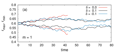
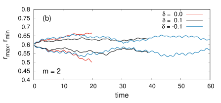
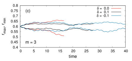
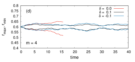
Figure 1: Time dependence of the maximum and minimum values of the radial coordinate of the free surface in slightly noncircular centrifuges for different azimuthal numbers $m$ of the bottom deviations and different detunings $\delta$ of the angular velocity of rotation from the corresponding resonant values.

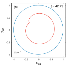
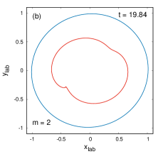
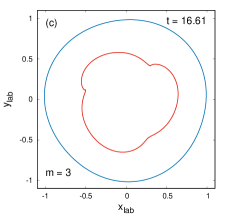
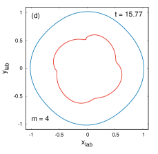
Figure 2: Formation of singularities on the free surface for $\delta=0$ and different $m$.

IV New application: waves in centrifuges

Before proceeding to new numerical results, we consider linearized equations of motion for surface waves in a partially filled, perfectly circular centrifuge (of unit radius and unit angular velocity) under the condition of relatively small gravity force ($g/\Omega^{2}R\ll 1$ in dimensional variables). We will use polar coordinates $r$ and $\chi$, so that $x+iy=r\exp(i\chi)$. In this case, the unknown functions are the small deviation of the free boundary $\eta(\chi,t)=[r(\chi,t)-c]$ from the equilibrium radius $0<c<1$ and the boundary value $\psi(\chi,t)$ of the velocity field potential. The generalized Bernoulli equation and the kinematic boundary condition on the free boundary in the main approximation are as follows (for $\Gamma=0$):

$$\psi_{t} = c\eta-2\hat{\mathfrak{R}}\psi-cg(t)\sin(\chi+t),$$ (35)

$$\eta_{t} = c^{-1}\hat{\mathfrak{R}}\psi_{\chi},$$ (36)

where the operator $\hat{\mathfrak{R}}$ (an analog of the operator $\hat{\sf R}_{\alpha}$ ) is diagonal in the discrete Fourier representation:

$${\mathfrak{R}}_{m}=i\frac{(1-c^{2m})}{(1+c^{2m})}=i\tanh(m\ln(1/c))\equiv i\sigma_{m}.$$ (37)

The relation $\theta(\chi,t)=\hat{\mathfrak{R}}\varphi(\chi,t)$ for $r=c$ arose from the fact that the fulfillment of the kinematic condition on the container wall is ensured by equality

$$\phi_{m}=A_{m}(t)r^{m}e^{im\chi}+\bar{A}_{m}(t)r^{-m}e^{-im\chi}.$$ (38)

In the case of $g=const$, a particular solution of the inhomogeneous linear system (35), (36) has the form

$$\psi_{\rm st} = \frac{cg}{(1+\sigma_{1})}\cos(\chi+t),$$ (39)

$$\eta_{\rm st} = \frac{-\sigma_{1}g}{(1+\sigma_{1})}\sin(\chi+t).$$ (40)

It corresponds to the stationary state in the laboratory coordinate system (see [43] for details). Equations (35) and (36) also yield an expression for the eigenfrequencies (the “dispersion law”; incidentally, we note that, in [43], the dispersion equation was derived in a nonrotating system, and this is probably why the answer was not brought to such a simple formula)

$$\omega_{m}=\sigma_{m}+\sqrt{\sigma_{m}^{2}+m\sigma_{m}}\,,$$ (41)

here positive $m$ correspond to leading waves, and negative $m$, to lagging waves (in laboratory coordinates). It is clear that if perturbations with azimuthal number $m$ and relative rotation speed $\Delta\approx\omega_{m}/m$ are introduced into the system, then one should observe a resonant growth of the corresponding harmonic. Such perturbations are most easily implemented by slightly distorting the shape of the centrifuge and forcing it to rotate with frequency of about $1+\Delta$, rather than with frequency $\Omega=1$. In the numerical examples shown in Figs. 1 and 2, such a regime is provided by the function

$$Z(\zeta,t)=\exp[i(-\omega_{-m}/m+\delta)t]e^{i\zeta}[1+\epsilon e^{im\zeta}]$$ (42)

with $\epsilon=0.02$ for $m=1,2,3,4$. The detuning from the resonance was fixed by the parameter $\delta$. As the initial conditions, we took the functions $\rho=0$ and $\psi=0$, and the initial value $\alpha_{0}=-\ln(0.6)$ gave an approximately circular shape of the free boundary with an average radius of $c\approx 0.6$. In this series of numerical experiments, we used a dimensionless gravity field of $g=0.02$.

Figures 1 and 2 show that there really was a resonant growth of waves accompanied by an enhancement of their nonlinearity and ending with the formation of a singularity on the free surface. In real conditions, this would mean the beginning of the transition of the flow to a three-dimensional turbulent regime.

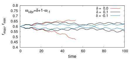
Figure 3: The maximum and minimum values of the radial coordinate of the free surface as a function of time for vertical vibration of the axis of a circular centrifuge with effective gravity force $g(t)=0.02-0.01\cos(\omega_{\rm vibr}t)$.

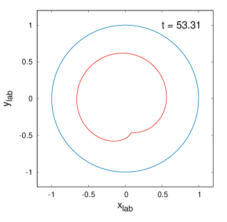
Figure 4: Formation of a singularity on the free surface in a circular centrifuge with a vertically vibrating axis for a resonant value of the vibration frequency.

Another possibility of introducing resonant perturbations is given by the vertical vibrations of the axis of rotation, which lead to the dependence

$$g(t)=g_{0}+A\cos(\omega_{\rm vibr}t).$$

Such perturbations act most effectively on the harmonics with $m=\pm 1$, even in the case of a perfectly circular container, as follows from the approximate equations (35) and (36). The resonance frequencies are given by the formula $\omega_{\rm vibr}=1\pm\omega_{\pm 1}$. The corresponding examples are illustrated in Figs. 3 and 4.

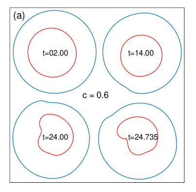
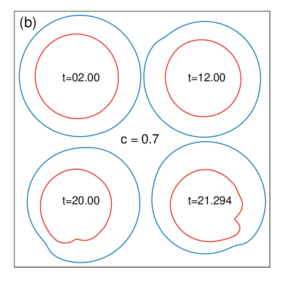
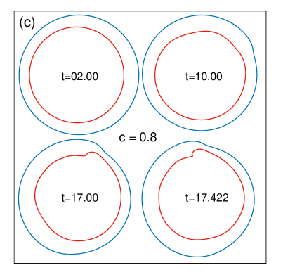
Figure 5: Formation of a singularity on the free surface in a centrifuge deformed according to formula (43) with $m=1$, $C_{1}=0.9$, and $C_{2}=0.7$ for three values of the initial radius.

Figure 6: Formation of a singularity on the free surface in a centrifuge deformed according to formula (43) with $m=2$, $C_{1}=0.9$, and $C_{2}=0.9$.

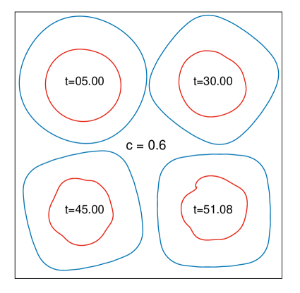
Figure 7: Formation of a singularity on the free surface in a centrifuge deformed from a circle to a square according to formula (46).

To demonstrate the full potential of the method, in Figs. 5 and 6 we show examples of the evolution of the free surface in a deformable centrifuge with a cross-sectional area varying (decreasing) with time. In these experiments, $g=0.1$, and the shape of the container corresponded to the analytic function

$$Z(\zeta,t)=\exp\Big{[}i\zeta+id(t)\ln\Big{(}\frac{1+C_{1}e^{im\zeta}}{1-C_{2}e^{im\zeta}}\Big{)}-0.5\pi d(t)\Big{]},$$ (43)

where the measure of deviation from circular shape was given by the expression $d(t)=0.1[1-\exp(-0.04t)]$. In Fig. 5, the parameters are $m=1$, $C_{1}=0.9$, and $C_{2}=0.7$. In Fig. 6, we took $m=2$, $C_{1}=0.9$, and $C_{2}=0.9$. At the initial time, this was a circularly symmetric configuration with the radius of the free surface $c$. Then, part of the bottom of the container was seemingly raised along the radius, thus forming $m$ regions with “smaller depth.” In this case, the decrease in the container area was accompanied by the appearance of an additional counterclockwise circular potential stream with parameter $\Gamma(t)$. Singularities (overturning angles) were formed on the crest of a growing wave near the point where the stream passed from smaller to larger depth.

Finally, Fig. 7 shows the deformation of the initially circular container to a shape intermediate between a circle and a square (for $g=0.1$, $c=0.6$). In this numerical experiment, we used the expansion of the corresponding elliptic integral up to the fourth order,

$$\int_{0}^{z}\frac{dz}{\sqrt{1-z^{4}}}\approx zE_{4}(z^{4}),$$ (44)

$$E_{4}(\mu)=\Big{(}1+\frac{\mu}{10}+\frac{\mu^{2}}{24}+\frac{5\mu^{3}}{16\cdot 13}+\frac{35\mu^{4}}{128\cdot 17}\Big{)},$$ (45)

to construct the function

$$Z(\zeta,t)=[1-0.1\tilde{d}(t)]e^{i\zeta}E_{4}\big{(}\tilde{d}(t)\exp(4i\zeta)\big{)},$$ (46)

where $\tilde{d}(t)=0.8[1-\exp(-0.04t)]$. In this case, a singularity was also formed. However, if, instead of the factor $[1-0.1\tilde{d}(t)]$, we took the factor $[1-0.2\tilde{d}(t)]$, which resulted in a more significant decrease in the container area and the hollow domain in it after deformation, then (for $c=0.6$) the waves on the free surface remained smooth for a long time and did not show a tendency to form sharp overturning crests (these results are not shown). There is yet no complete understanding of the reasons for such behavior.

V Conclusions

Thus, the main result of this work is the development and application of the method of composite conformal mapping to describe the dynamics of waves on the free surface of an ideal incompressible fluid in partially filled flat centrifuges of complex shape. Just as in previous applications, the method has demonstrated high accuracy and efficiency. True, so far we cannot say that all questions have been exhausted. For example, it is not yet clear how to modify the method in the case when a relatively small hollow domain (a hollow vortex for $\Gamma\neq 0$) moves far from the origin during its dynamics so that the origin turns out to be filled with a fluid. Obviously, a conformal mapping of the type $Z(\zeta)=\exp(i\zeta)$, which has a singularity at $Z=0$ (or at any other previously fixed point), fails to work in this case.

However, even in the existing version, the method can solve many interesting problems. It is quite clear that the examples presented here are far from exhausting the entire variety of possible wave structures and their dynamics in rotating systems with nontrivial geometry.

References

- (1) L. V. Ovsyannikov, in Dynamics of Continuous Media (Nauka Novosibirsk, 1973), No. 15, p. 104 [in Russian].
- (2) L. V. Ovsjannikov, Arch. Mech. 26, 407 (1974) .
- (3) A. I. Dyachenko, E. A. Kuznetsov, M. D. Spector, and V. E. Zakharov, Phys. Lett. A 221, 73 (1996).
- (4) A. I. Dyachenko, Y. V. Lvov, and V. E. Zakharov, Physica D 87, 233 (1995).
- (5) A. I. Dyachenko, V. E. Zakharov, and E. A. Kuznetsov, Plasma Phys. Rep. 22, 829 (1996).
- (6) A. I. Dyachenko, Doklady Math. 63, 115 (2001).
- (7) V. E. Zakharov, A. I. Dyachenko, and O. A. Vasilyev, Eur. J. Mech. B/Fluids 21, 283 (2002).
- (8) A. I. Dyachenko and V. E. Zakharov, Pis’ma v ZhETF 81, 318 (2005).
- (9) V. E. Zakharov, A. I. Dyachenko, and A. O. Prokofiev, Eur. J. Mech. B/Fluids 25, 677 (2006).
- (10) A. I. Dyachenko and V. E. Zakharov, Pis’ma v ZhETF 88, 356 (2008).
- (11) W. Choi and R. Camassa, J. Engng Mech. 125, 756 (1999).
- (12) Y. A. Li, J. M. Hyman, abd W. Choi, Stud. Appl. Math. 113, 303 (2004).
- (13) R. V. Shamin, Dokl. Math. 73, 112 (2006).
- (14) R. V. Shamin, Dokl. Phys. 77, 118 (2008).
- (15) R. V. Shamin, Dokl. Phys. 81, 436 (2010).
- (16) V. E. Zakharov and R. V. Shamin, JETP Lett. 91, 62 (2010).
- (17) V. E. Zakharov and R. V. Shamin, JETP Lett. 96, 66 (2012).
- (18) D. Chalikov and D. Sheinin, J. Comput. Phys. 210, 247 (2005).
- (19) D. Chalikov, Phys. Fluids 21, 076602 (2009).
- (20) A. V. Slyunyaev, J. Exp. Theor. Phys. 109, 676 (2009).
- (21) W. Choi, Math. Comp. Simulat. 80, 29 (2009).
- (22) S. A. Dyachenko, P. M. Lushnikov, and A. O. Korotkevich, JETP Lett. 98, 675 (2013).
- (23) N. M. Zubarev and E. A. Kochurin, JETP Lett. 99, 62 (2014).
- (24) P. M. Lushnikov, J. Fluid Mech. 800, 557 (2016).
- (25) M. R. Turner and T. J. Bridges, Adv. Comput. Math. 43, 947 (2016).
- (26) M. R. Turner, J. Fluids Struct. 64, 1 (2016).
- (27) M. G. Blyth and E. I. Parau, J. Fluid Mech. 806, 5 (2016).
- (28) P. M. Lushnikov, S. A. Dyachenko, and D. A. Silantyev, Proc. R. Soc. A 473(2202), 2017019 (2017).
- (29) A. I. Dyachenko, P. M. Lushnikov, and V. E. Zakharov, J. Fluid Mech. 869, 526 (2019).
- (30) A. I. Dyachenko, S. A. Dyachenko, P. M. Lushnikov, and V. E. Zakharov, J. Fluid Mech. 874, 891 (2019).
- (31) S. A. Dyachenko, J. Fluid Mech. 860, 408 (2019).
- (32) T. Gao, A. Doak, J.-M. Vanden-Broeck, and Zh. Wang, Eur. J. Mech./B Fluids 77, 98 (2019).
- (33) M. V. Flamarion, P. A. Milewski, and A. Nachbin, Stud. Appl. Math. 142, 433 (2019).
- (34) D. Kachulin, A. Dyachenko, and A. Gelash, Fluids 4, 83 (2019).
- (35) V. P. Ruban, Phys. Rev. E 70, 066302 (2004).
- (36) V. P. Ruban, Phys. Lett. A 340, 194 (2005).
- (37) V. P. Ruban, Phys. Rev. E 77, 037302 (2008).
- (38) V. P. Ruban, Phys. Rev. E 77, 055307(R) (2008).
- (39) V. P. Ruban, Phys. Rev. E 78, 066308 (2008).
- (40) V. P. Ruban, JETP Lett. 93, 195 (2011).
- (41) V. P. Ruban, J. Exp. Theor. Phys. 114, 343 (2012).
- (42) V. P. Ruban, JETP Lett. 95, 486 (2012).
- (43) O. M. Phillips, J. Fluid Mech. 7, 340 (1960).
- (44) A. A. Ivanova, V. G. Kozlov, and A. V. Chigrakov, Fluid Dynamics 39, 594 (2004).
- (45) A. A. Ivanova, V. G. Kozlov, and D. A. Polezhaev, Fluid Dynamics 40, 297 (2005).
- (46) http://www.fftw.org