HERA data and collinearly-improved BK dynamics

Abstract

Within the framework of the dipole factorisation, we use a recent collinearly-improved version of the Balitsky-Kovchegov equation to fit the HERA data for inclusive deep inelastic scattering at small Bjorken $x$. The equation includes an all-order resummation of double and single transverse logarithms and running coupling corrections. Compared to similar equations previously proposed in the literature, this work makes a direct use of Bjorken $x$ as the rapidity scale for the evolution variable. We obtain excellent fits for reasonable values for the four fit parameters. We find that the fit quality improves when including resummation effects and a physically-motivated initial condition. In particular, the resummation of the DGLAP-like single transverse logarithms has a sizeable impact and allows one to extend the fit up to relatively large photon virtuality $Q^{2}$.

1 Introduction

Derived via systematic approximations within perturbative QCD, the Colour Glass Condensate (CGC) effective theory [1, 2, 3, 4, 5] is a powerful framework for computing high-energy processes in the presence of non-linear effects associated with high parton densities. There are intense ongoing efforts towards extending this effective theory to next-to-leading order (NLO) accuracy, as required by realistic applications to phenomenology [6, 7, 8, 9, 10, 11, 12, 13, 14, 15, 16, 17, 18, 19]. These efforts refer both to the Balitsky-JIMWLK equations [20, 21, 22, 23, 24, 25, 26], which govern the high-energy evolution of the scattering amplitudes, and to the impact factors, which represent cross-sections at relatively low energy. The first NLO results, obtained more than a decade ago [6, 7, 8], refer to the Balitsky-Kovchegov (BK) equation [20, 27]. The latter is a non-linear equation emerging from the B-JIMWLK hierarchy in the limit of a large number of colours ($N_{c}\to\infty$). It describes the evolution of the elastic scattering amplitude between a colour dipole and a dense hadronic target. Via appropriate factorisation schemes, like the “dipole factorisation” or the “hybrid factorisation” [28], the BK equation also governs the high-energy evolution of the cross-sections for processes of phenomenological interest, like deep inelastic scattering (DIS) at small Bjorken $x$, or forward particle production in proton-nucleus collisions.

A few years after the full NLO BK equation was first presented [8], its numerical study in [29] showed that it is unstable, as anticipated in [30, 31]. Similar problems had been identified, and cured [32, 33, 34, 35, 36, 37], for the NLO version of the BFKL equation [38, 39, 40] — the linearised version of the BK equation, valid for weak scattering. The origin of this difficulty has been clearly identified, both numerically [29] and conceptually [31, 41]: it is associated with large and negative NLO corrections enhanced by a double “anti-collinear” logarithm, generated by integrating out gluon emissions with small transverse momenta (see Sect. 2). Such double-logarithmic corrections spoil the convergence of the fixed-order perturbative expansion of the high-energy evolution, unless they are properly resummed to all orders. Refs. [31, 41] proposed two different strategies for resumming this series of double-logarithmic corrections to all orders.

At a first sight, these strategies seemed to be successful, leading to stable evolution equations [41, 42] and allowing for good fits to the small-$x$ HERA data [43, 44]. However, a recent study [45] revealed some inconsistencies in the original analyses in [31, 41, 43, 44]. In particular, there was a confusion concerning the meaning of the rapidity variable which plays the role of the evolution time. The variable which a priori enters the perturbative calculations at NLO [8] and in the resummed equations proposed in [31, 41] is the rapidity $Y\equiv\ln(s/Q_{0}^{2})$ of the dipole projectile, with $s$ the centre-of-mass energy squared and $Q_{0}$ a typical transverse momentum scale for the target. It is different from the rapidity $\eta\equiv\ln(1/x)$ of the hadronic target, which is the variable used in DIS (see Sect. 2 for details). When translated to this physical variable, the results of the original resummations in [31, 41] show a strong scheme dependence, preventing any meaningful phenomenological applications [45]. The success of the corresponding fits to the HERA data [43, 44] was rather fortuitous and can be attributed to several factors: (i) these fits blindly assumed the physical rapidity variable $\eta=\ln(1/x)$ (although this was inconsistent with the resummation scheme), (ii) the rapidity interval over which one can probe high-energy evolution is relatively limited making it delicate to critically probe the effects of resummation. In other words, even though the fits can hint at an evolution being better than another (e.g. via a better $\chi^{2}$, or more physical fit parameters), it remains difficult to draw a firm conclusion.

To overcome these difficulties, Ref. [45] proposed a reorganisation of perturbation theory in which the evolution time is the physical rapidity $\eta$. This program lead to a new version of “collinearly-improved BK equation”, shown below in Eq. (6). This equation is non-local in rapidity. In that sense it looks formally similar to the equation proposed in [31] but these two equations are fundamentally different: (i) the evolution variable, $\eta$, occurring in Eq. (6) is the physical rapidity $\ln(1/x)$, and not the rapidity of the dipole projectile; (ii) the rapidity shift in Eq. (6) accounts for an all-order resummation of double collinear logarithms, and not anti–collinear (see Sect. 2). The collinear logarithms are generated by gluon emissions with relatively large momenta. Such emissions are atypical in the context of DIS. Moreover, they are partially suppressed by non-linear effects, so their resummation is somewhat less critical. As a consequence, a comparison between various resummation prescriptions shows only little scheme dependence [45], at the level of the expected perturbative accuracy of the resummed equation.

The evolution equation we use in this work, Eq. (6), actually goes beyond the original proposal from Ref. [45] by additionally including a class of DGLAP-like single transverse logarithms (both collinear and anti-collinear) which appears in the NLO BK equation. While in principle one can also include [45] the full set of NLO BK corrections in our evolution equation, this is numerically cumbersome (see however [42]) and it goes beyond the scope of this Letter. Instead, we directly confront the relatively simple equation (6) with the most recent HERA data [46] for inclusive DIS at small Bjorken $x\leq 0.01$. This dataset includes more data points as compared to the one used in previous fits [43, 44].

We use the fits to test the resummation of the aforementioned double logs and single transverse logarithms as well as various prescriptions for the running of the QCD coupling which enters the BK equation. We study two models for the initial condition to the BK equation: the simple Golec-Biernat and Wüsthoff (GBW) model [47, 48] and a a running-coupling version of the McLerran-Venugopalan (MV) model [49]. Both models include two free parameters which are fitted to the experimental data. Two additional parameters (leaving aside the quark masses that we keep fixed) are associated with our ansatz for the running coupling and with the overall normalisation of the DIS cross-section.

With this setup, we find a good overall agreement with the HERA data at small $x$. Furthermore, it appears that the physically-motivated MV model with running coupling is preferred over the GBW model, with the former giving both better $\chi^{2}$ and more reasonable parameter values than the latter. As with earlier studies, the fits appear to favour an initial condition for the dipole scattering amplitude with a fast and abrupt approach to the unitarity limit. This is the main reason why better fits are obtained with the running coupling version of the MV model as compared to its original fixed-coupling version [49]. This finding is also in agreement with the fact that previous fits [50, 51] using the original MV model favoured a modified dependence of the initial amplitude on the dipole size, decreasing like $r^{2\gamma_{0}}$ with $\gamma_{0}>1$. Another interesting observation of our fits is that the inclusion of the DGLAP-like single logarithms significantly improves the description of the data at large $Q^{2}$, allowing for good descriptions up to maximum $Q^{2}$ of 400 GeV².

This Letter is organised as follows. Sect. 2 provides a qualitative and (hopefully) pedagogical summary of the arguments justifying the replacement of the original collinear-improved BK equation formulated in terms of the rapidity of the dipole projectile [31, 41], by a new version formulated in terms of the rapidity of the hadron target, or Bjorken $x$. (We refer to Ref. [45] for more details.) Sect. 3 discusses the main physical consequences of the various resummations on the solution to the collinearly-improved BK equation. Finally, Sect. 4 presents the main original results of this paper: the setup and the results for the fits together with their physical discussion.

2 Collinearly-improved BK evolution in the target rapidity

The main difference between our present approach and previous saturation fits to DIS refers to our specific choice of evolution equation used to describe the evolution of the dipole $S$-matrix with increasing energy. More precisely, we use a collinearly-improved version of the BK equation — recently proposed in [45] — in which the rapidity variable playing the role of the evolution time is the proton rapidity $\eta=\ln(1/x)$, with $x$ the standard Bjorken variable. This contrasts previous studies (see e.g. [8, 31, 41, 43]) where the evolution was formulated in terms of the rapidity $Y$ of the dipole projectile. Beyond leading order [20, 27], the choice of $\eta$ over $Y$ has important consequences. To make this clear, we first summarise the main findings of [45] which are relevant for the fit to DIS data described in the next section.

Basic kinematics, target and projectile rapidity

We use a frame in which the virtual photon, $\gamma^{*}$, is an energetic right-mover with (light-cone) 4-momentum $q^{\mu}\equiv(q^{+},q^{-},\bm{q}_{\perp})=(q^{+},-\frac{Q^{2}}{2q^{+}},\bm{0}_{\perp})$, whereas the proton target is a left-mover with $P^{\mu}=\delta^{\mu-}P^{-}$. In the high-energy or small Bjorken $x$ regime,

$$x\equiv\,\frac{Q^{2}}{2P\cdot q}=\,\frac{Q^{2}}{2P^{-}q^{+}}\,\ll\,1\,,$$ (1)

the coherence time $\Delta x^{+}\simeq 2q^{+}/Q^{2}$ of the virtual photon, i.e. the typical lifetime of its quark-antiquark ($q\bar{q}$) fluctuation, is much larger than the longitudinal extent $1/P^{-}$ of the target. This justifies the use of the dipole picture in which the $\gamma^{*}$ fluctuates into a $q\bar{q}$ colour dipole long before the collision, which then scatters inelastically off the proton. Via the optical theorem, the total dipole-hadron scattering cross-section is related to the $S$-matrix for the elastic scattering. At high energy, one can work in the eikonal approximation where the transverse coordinates $\bm{x}$ of the quark and $\bm{y}$ of the antiquark are not affected by the collision.

The elastic $S$-matrix $S_{\bm{x}\bm{y}}$ also depends on the rapidity difference between the dipole and the proton through the high-energy evolution. The physical picture of this evolution and its analytical description depend on how the total energy is divided between the (dipole) projectile and the (proton) target i.e. upon the choice of the “dipole frame” in which one is working. It is useful to consider the two extreme situations: the “target frame”, in which most of the total energy (and hence the whole high-energy evolution) is carried by the proton, and the “projectile frame”, where the energy is mostly carried by the dipole (and the high-energy evolution is encoded in the dipole wavefunction). Importantly the rapidity variable which represents the “evolution time” for the high-energy evolution, is different in these two situations:

target rapidity: $$\eta\equiv\,\ln\frac{P^{-}}{|q^{-}|}\,=\,\ln\frac{2q^{+}P^{-}}{Q^{2}}\,=\,\ln\frac{1}{x}$$ (2)

dipole rapidity: $$Y\equiv\,\ln\frac{q^{+}}{q_{0}^{+}}=\,\ln\frac{2q^{+}P^{-}}{Q_{0}^{2}}=\,\ln\frac{1}{x}+\ln\frac{Q^{2}}{Q_{0}^{2}}=\eta+\rho$$ (3)

For the target rapidity, the typical gluon from the proton which interacts with the dipole has a longitudinal momentum $k^{-}={Q^{2}}/{2q^{+}}=|q^{-}|$, and hence a longitudinal extent $\sim 1/k^{-}$ of the order of the lifetime $\Delta x^{+}$ of the $q\bar{q}$ pair. For the projectile rapidity, the softest dipole to participate in the collision has a longitudinal momentum $q_{0}^{+}=Q_{0}^{2}/2P^{-}$ — i.e. a lifetime ${2q_{0}^{+}}/{Q_{0}^{2}}$ equal to the longitudinal extent $1/P^{-}$ of the proton —, where the scale $Q_{0}\ll Q$ is the transverse momentum scale for the onset of unitarity (multiple scattering) effects in the (unevolved) proton. The two rapidities differ by $\rho\equiv\ln({Q^{2}}/{Q_{0}^{2}})$ which is large when $Q\gg Q_{0}$.

The non-linear effects associated with the high gluon density are described differently in the two frames. In the target frame, soft gluon emissions occur in the proton wavefunction which is a dense environment. Accordingly, these emissions are modified by non-linear effects like gluon recombinations. The non-linear evolution of the dense hadron wavefunction has been computed only to leading order, yielding the (functional) JIMWLK equation [21, 22, 23, 24, 25, 26]. Conversely, in the dipole frame one views the evolution as successive, soft, gluon emissions within the dipole wavefunction, a dilute hadronic system. Gluon emissions from the dipole occur like in the vacuum and non-linear effects exclusively refer to multiple scattering. This leads to the Balitsky hierarchy (and the BK equation), currently known to NLO accuracy [8, 9, 10, 11, 12]. Since our purpose in this work is to go beyond LO accuracy, we systematically use the dipole frame in what follows.

Time ordering and collinear improvements in $Y$ (dipole frame)

Besides being less suited for applications to DIS, the evolution with $Y$ has a more severe conceptual drawback: the typical emissions contributing to this evolution at leading order can violate proper time ordering, that is, the condition that the formation time of a daughter gluon be smaller than the lifetime of its parent. To understand this, we first recall that, when $Q^{2}\gg Q^{2}_{0}$, the typical emissions associated with the high-energy evolution of the dipole wavefunction are strongly ordered both in longitudinal momenta ($k^{+}$) and in transverse momenta ($k_{\perp}$):

$$q^{+}\gg k_{1}^{+}\gg k_{2}^{+}\gg\dots\gg q_{0}^{+}\,,\qquad Q^{2}\gg k_{1\perp}^{2}\gg k_{2\perp}^{2}\gg\dots\gg Q_{0}^{2}\,.$$ (4)

This corresponds to soft and collinear emissions which yield the dominant, double-logarithmic, contributions proportional to powers of $\bar{\alpha}_{s}Y\rho$. However, an explicit calculation of the relevant Feynman graphs shows [41] that this double-logarithmic enhancement only holds so long as the gluon lifetimes are ordered as well:

$$\frac{2q^{+}}{Q^{2}}\gg\frac{2k_{1}^{+}}{k_{1\perp}^{2}}\gg\frac{2k_{2}^{+}}{k_{2\perp}^{2}}\gg\dots\gg\frac{2q_{0}^{+}}{Q_{0}^{2}}\,.$$ (5)

This condition reduces the rapidity phase-space available for the evolution from $Y$ to $Y-\rho\equiv\eta$. The condition Eq. (5) is already violated (due to the emission of daughter gluons with sufficiently soft $k_{\perp}$) in the LO BK evolution which resums an infinite series in $\bar{\alpha}_{s}Y\rho$, instead of the correct series in powers of $\bar{\alpha}_{s}(Y-\rho)\rho$. The difference between the two corresponds to an alternating series of double “anti-collinear” logarithms proportional to $\bar{\alpha}_{s}\rho^{2}$ which spoil the convergence of the perturbative expansion in $Y$. In particular, the NLO BK equation includes the first (negative) contribution proportional to $\bar{\alpha}_{s}\rho^{2}$ [8] which makes the evolution unstable [29] and hence unsuitable for physical studies.

To overcome this difficulty, it was originally proposed [31, 41] to enforce time-ordering directly in the dipole frame evolution. Two “collinearly improved” BK equations have been proposed: in the first [31] the evolution is non-local in rapidity and has the same kernel as at LO, while in the second [41] the evolution is local in $Y$, but both the kernel and the initial condition receive corrections to all orders in $\bar{\alpha}_{s}\rho^{2}$. Both methods allow for a faithful resummation of the dominant series in powers of $\bar{\alpha}_{s}\rho^{2}$, but the subleading terms (proportional to powers of $\bar{\alpha}_{s}^{k}\rho^{2}$ with $k\geq 2$) are not under control. At a first sight, both strategies appear to be successful: the respective equations are stable [41, 42], they can be extended to full NLO accuracy [42], and moreover they allow for good fits to the HERA data for DIS at small $x$ [43, 44].

Recasting dipole evolution in terms of $\eta$

A more recent study has revealed that these apparent successes were in fact deceiving [45]. The numerical studies in [43, 44, 42] have been presented in terms of $Y$ instead of the physical rapidity $\eta=Y-\rho=\ln(1/x)$, and in the DIS fits in [43, 44], the variable $Y$ has been abusively interpreted as $\ln(1/x)$. The correct procedure would require to first transform the results from $Y$ to $\eta$ by a simple change of variables, before attempting a physical interpretation or a fit to the data. When following this correct procedure, one finds [45] an unacceptably large resummation-scheme dependence. For example when solved with the same initial condition the two “collinearly-improved” BK equations introduced in [31] and [41] yield very different predictions for the evolution in $\eta$. More generally, different choices for the “rapidity shift” in the non-local equation in $Y$, albeit equivalent to DLA, lead to very different predictions for the saturation exponent $\lambda_{s}$ [45]. This strong scheme dependence forbids any physical interpretation of the results. It demonstrates that the uncontrolled, subleading, double-logarithmic corrections — which generally differ from one resummation scheme to another — are numerically important.

The problem is further complicated by the fact that the resummed BK evolution in $Y$ cannot be formulated as a genuine initial-value problem. The non-local equation introduced in [31] must be solved as a boundary-value problem (on a line of constant $Y-\rho$) which seriously complicates even numerical studies of the equation. Moreover, even if the local equation with a resummed kernel [41] does admit an initial-value formulation, the corresponding initial condition must itself be resummed to account for double-logarithmic corrections to all orders, a task which appears to be intractable beyond strict DLA.

These difficulties with the evolution in $Y$ can be avoided altogether by using $\eta$ as an “evolution time” [45]. This choice has some obvious virtues in practice: $\eta=\ln(1/x)$ is the right variable to be used in phenomenological studies of DIS and, clearly, a boundary-value condition formulated at constant $Y-\rho$ becomes an initial condition for the evolution in $\eta$. Most importantly, one can show that the evolution in $\eta$ naturally ensures the proper time ordering of the successive emissions.

Instead of computing directly the target evolution in $\eta$ which would be delicate in the presence of saturation, Ref. [45] proposed to reformulate the dipole evolution in $Y$, computed in pQCD, as an evolution in $\eta$ via the change of variables $Y\equiv\eta+\rho$. Such a change of variables is unambiguous in perturbation theory and has been used [45] to obtain the NLO BK equation in $\eta$ from the respective equation in $Y$ [8].

Resummation of atypical collinear double logarithms

When using $\eta$ as an evolution variable, the BK equation is not affected by the large anti-collinear logarithms that were present in the evolution in $Y$. This is a consequence of time ordering, Eq. (5), being automatically satisfied for the evolution in $\eta$. Furthermore, (5) also guarantees that typical anti-collinear emissions — i.e. those strongly ordered in transverse momentum according to (4) — automatically satisfy the proper ordering in longitudinal momentum $k^{+}$ (cf. (4) again).

However, even with the proper time-ordering, the correct ordering in $k^{+}$ can still be violated by a series of collinear emissions with a strong transverse momentum ordering opposite to that of Eq. (4). These violations yield double-logarithmic corrections to the BK kernel, starting at NLO (cf. [45]). In principle, this problem is as severe as the one of time-ordering violations in the evolution in $Y$: these collinear logarithms have to be resummed to all orders in the evolution in $\eta$, as the anti-collinear were resummed in the evolution in $Y$. However, these collinear emissions, where the daughter gluon has a much larger transverse momentum than the parent one are atypical in the context of DIS. One can further show that they are also strongly suppressed by saturation which freezes the evolution for emissions with sufficiently soft transverse momentum.

The NLO evolution in $\eta$ nonetheless has a contribution from collinear logarithms which, albeit suppressed, eventually translates into an instability at large-enough rapidity. In practice one would therefore resum it to all orders (see [45]) using a rapidity shift leading to a non-local evolution in $\eta$ (see Eq. (6) below). As for the resummations in $Y$, this resummation scheme is not unique beyond DLA. But unlike what happens with the resummations in $Y$, the scheme dependence for the resummations in $\eta$ is reasonably small, in agreement with the expected perturbative accuracy of the resummed equations. For example, choosing different resummation schemes (e.g. by varying the $\eta$ shift in (6)), one finds a small impact on the saturation exponents, comparable with missing perturbative contributions of ${\cal{O}}(\bar{\alpha}_{s}^{2})$.

The collinearly-improved BK equation in $\eta$

We are finally in a position to present the evolution equation in the target rapidity, $\eta$ which reads

$$\frac{\partial{S}_{\bm{x}\bm{y}}(\eta)}{\partial\eta}=\int{\rm d}^{2}\bm{z}\frac{\bar{\alpha}_{s}(r_{\min})}{2\pi}\frac{(\bm{x}-\bm{y})^{2}}{(\bm{x}-\bm{z})^{2}(\bm{z}-\bm{y})^{2}}\,\left[\frac{r^{2}}{\bar{z}^{2}}\right]^{\pm A_{1}}\big{[}{S}_{\bm{x}\bm{z}}(\eta\!-\!\delta_{\bm{x}\bm{z};r}){S}_{\bm{z}\bm{y}}(\eta\!-\!\delta_{\bm{z}\bm{y};r})-{S}_{\bm{x}\bm{y}}(\eta)\big{]},$$ (6)

where $\bm{z}$ is the transverse position of the gluon emitted by either the quark or the antiquark. In the large-$N_{c}$ approximation, implicit in (6), this can be viewed as the splitting of the original dipole $(\bm{x},\,\bm{y})$ into two daughter dipoles $(\bm{x},\,\bm{z})$ and $(\bm{z},\,\bm{y})$. The other notations are explained below. Compared to the LO BK equation (in $\eta$) a few key differences are worth noting:

(i) the use of the one-loop running coupling $\bar{\alpha}_{s}(r_{\min})$ with the running scale set by the size $r_{\min}$ of the smallest dipole: $r_{\min}\equiv\min\{|\bm{x}-\bm{y}|,|\bm{x}-\bm{z}|,|\bm{z}-\bm{y}|\}$. Alternative schemes are discussed in the next section.

(ii) the rapidity shifts in the arguments of the $S$-matrices for the daughter dipoles ensure the resummation of the leading double logarithms associated with the $k^{+}$ ordering. They are given by

$$\delta_{\bm{x}\bm{z};r}\equiv\max\left\{0,\ln\frac{r^{2}}{|\bm{x}\!-\!\bm{z}|^{2}}\right\}$$ (7)

with $r\equiv|\bm{x}-\bm{y}|$, and similarly for $\delta_{\bm{z}\bm{y};r}$. They are non-zero only for emissions in which one of the daughter dipoles is (much) smaller than the parent one, in agreement with our earlier discussion about collinear logarithms. Expanding (6) to first non-trivial order in $\delta$ would give the double-logarithmic contribution to the BK kernel at NLO which eventually yields an instability unless properly resummed as in (6).

(iii) Eq. (6) also includes the resummation of the first set of single DGLAP logarithms (either collinear, or anti-collinear), via the factor $\left[{r^{2}}/{\bar{z}^{2}}\right]^{\pm A_{1}}$, where $\bar{z}\equiv\min\{|\bm{x}-\bm{z}|,|\bm{z}-\bm{y}|\}$. The number $A_{1}=11/12$ is related to the DGLAP splitting function via the following Mellin transform:

$$\int_{0}^{1}{\rm d}z\,z^{\omega}\left[P_{\rm gg}(z)+\frac{C_{\rm F}}{N_{\rm c}}\,P_{\rm qg}(z)\right]=\frac{1}{\omega}-A_{1}+\mathcal{O}\left(\omega,\frac{N_{\rm f}}{N_{\rm c}^{3}}\right).$$ (8)

The singular piece $1/\omega$ generates the $\eta=\ln(1/x)$ logarithm contributing to the LO BK evolution, while the non-singular piece $(-A_{1})$ contributes at NLO and is enhanced by a single transverse logarithm $\ln({r^{2}}/{\bar{z}^{2}})$. The sign in the exponent, $\pm A_{1}$, is taken to be plus for an anti-collinear emission (${r^{2}}<{\bar{z}^{2}}$) and minus for a collinear one, so this factor is always suppressing the evolution.

Eq. (6) has to be solved as an initial value problem, albeit a somehow unusual one due to its non-locality in $\eta$. Indeed, since the shift introduces a dependence to rapidities smaller than $\eta$, if we want to start the evolution at some rapidity $\eta_{0}$ we should specify the initial condition for $\eta\leq\eta_{0}$. Our prescription is to assume a constant behaviour in $\eta$ (see Sect. 9 of Ref. [45]) i.e.

$${S}_{\bm{x}\bm{y}}(\eta<\eta_{0})={S}^{(0)}_{\bm{x}\bm{y}}\,.$$ (9)

With this prescription, Eq. (6) can be solved and used for DIS fits.

A final note concerns the perturbative accuracy of Eq. (6). We have argued that it includes all the NLO corrections enhanced by at least one transverse logarithm. Hence, from the viewpoint of a strict weak-coupling expansion, it is accurate up to pure NLO corrections, of $\mathcal{O}{(\bar{\alpha}_{s}^{2})}$ without any logarithmic enhancement. Furthermore, the resummation-scheme dependence of (6) is also coherent with missing ${\cal{O}}(\bar{\alpha}_{s}^{2})$ terms. It is possible to extend this equation to full NLO accuracy by adding the missing pure $\bar{\alpha}_{s}^{2}$ corrections. The resulting equation, which can be found in Ref. [45], is substantially more complex and we postpone its applications to DIS to future work.

3 Illustrating the impact of running coupling and resummation effects

Before turning to the description of inclusive DIS data, it is helpful to briefly illustrate how the various ingredients in the BK equation, namely running-coupling (RC) corrections and the resummation of transverse logarithms, affect the evolution in $\eta$. For this purpose, we choose a homogeneous target, i.e. take ${S}_{\bm{x}\bm{y}}(\eta)=S(\eta,r)$ with $r=|\bm{x}-\bm{y}|$, together with the simple Golec-Biernat–Wüsthoff (GBW) initial condition [47, 48]: $S_{0}(r)=\exp(-r^{2}Q_{0}^{2})$ with $Q_{0}^{2}=1\,{\rm GeV}^{2}$. This Gaussian Ansatz does not capture the proper behaviour for $r^{2}Q_{0}^{2}\ll 1$ but is enough for illustrating our points in this section.

Let us first discuss running-coupling effects. For the sake of the present discussion, we use

$$\bar{\alpha}_{s}(r)=\frac{1}{\bar{b}_{0}\ln\big{[}4/(r^{2}\Lambda^{2})\big{]}},$$ (10)

with $\bar{b}_{0}=0.75$ (corresponding to $n_{f}=3$) and $\Lambda=0.2$ GeV. The Landau pole is avoided by freezing the coupling at the value $\bar{\alpha}_{\rm sat}=0.67$. There is some freedom in implementing RC corrections in the BK equation and we consider two different prescriptions: the minimal dipole prescription, $\bar{\alpha}_{s}(r_{\min})$, where Eq. (10) is evaluated at $r=r_{\min}\equiv\min\{|\bm{x}-\bm{y}|,|\bm{x}-\bm{z}|,|\bm{z}-\bm{y}|\}$ and the BLM prescription (also dubbed as “fast apparent convergence” [43]), defined as

$$\bar{\alpha}_{\rm\scriptscriptstyle BLM}=\left[\frac{1}{\bar{\alpha}_{s}(|\bm{x}\!-\!\bm{y}|)}+\frac{(\bm{x}\!-\!\bm{z})^{2}-(\bm{z}\!-\!\bm{y})^{2}}{(\bm{x}\!-\!\bm{y})^{2}}\frac{\bar{\alpha}_{s}(|\bm{x}-\bm{z}|)-\bar{\alpha}_{s}(|\bm{z}-\bm{y}|)}{\bar{\alpha}_{s}(|\bm{x}-\bm{z}|)\bar{\alpha}_{s}(|\bm{z}-\bm{y}|)}\right]^{-1}.$$ (11)

Other prescriptions, not studied here, are also possible (see e.g. [6, 7, 8]). They all have in common that they reduce to $\bar{\alpha}_{s}(r_{\min})$ when one of the three dipoles is much smaller than the other two, as one can easily check for $\bar{\alpha}_{\rm\scriptscriptstyle BLM}$. This minimises the NLO correction to the BK equation proportional to the one-loop $\beta$-function.

Besides varying the prescription for the running coupling, we also aim to probe the effect of the resummation of transverse logarithms. Single logarithms can be switched off by removing the factor $\left[{r^{2}}/{\bar{z}^{2}}\right]^{\pm A_{1}}$ in Eq. (6), while to remove double transverse logarithms we set the $\eta$ shifts, $\delta_{\bm{x}\bm{z};r}$ and $\delta_{\bm{z}\bm{y};r}$, to zero.

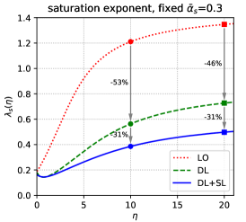
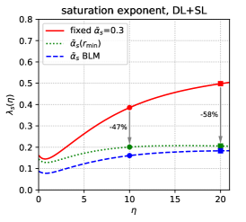
Figure 1: The saturation exponent $\lambda_{s}(\eta)$ extracted from solutions to Eq. (6) with GBW initial condition and with 3 different choices for the QCD coupling: fixed coupling $\bar{\alpha}_{s}=0.3$ (left), RC $\bar{\alpha}_{s}(r_{\min})$ (middle), and RC $\bar{\alpha}_{\rm\scriptscriptstyle BLM}$ (right). In each of these 3 cases, we show results corresponding to LO, LO+DL, and LO+DL+SL, respectively (see text for details).

In practice, we solve Eq. (6) numerically up to $\eta=20$ and study the saturation exponent defined as

$$\lambda_{s}(\eta)\,\equiv\,\frac{{\rm d}\ln Q_{s}^{2}(\eta)}{{\rm d}\eta}\,,$$ (12)

with the saturation momentum $Q_{s}(\eta)$ numerically obtained from the condition that $S(\eta,r)=\tfrac{1}{2}$ when $r=2/Q_{s}(\eta)$. The rapidity range under study is not sufficient to reach the universal asymptotic behaviour but is representative for the actual range covered by the HERA data, $\eta\lesssim 10$.

Our results are presented in Fig. 1 for a fixed-coupling prescription as well as for our two RC prescriptions. In each case we show the saturation exponent for the LO BK equation without any transverse logarithm resummation (“LO”, dotted red), when double transverse logarithms are resummed (“DL”, dashed green) and when both double and single transverse logarithms are resummed (“DL+SL”, solid blue).

The first observation is that running coupling effects have a large impact, reducing the saturation exponent by $\sim$75% for both RC prescriptions at $\eta=10$ and even more at larger rapidities. The effect of resumming large transverse logarithms is smaller but still clearly visible: with RC, we see an additional $\sim 10-25\%$ reduction coming from the resummation of double logarithms and a $\sim 10-20\%$ reduction coming from single logarithms. (The effect is considerably larger when using a fixed coupling.) The fact that single-log effects are almost as large as double-log effects is most likely due to the fact that while the latter are only relevant for large dipole sizes — where they are reduced by saturation effects — the former have an impact on both large (collinear) and small (anti-collinear) dipoles.

Furthermore, one sees that, without the resummation of the transverse logarithms, $\lambda_{s}$ is still quite large (e.g. $\lambda_{s}(\eta=10)=0.26$ for rcBK with the BLM prescription). This seems to be still too large to optimally accommodate the small-$x$ HERA data. It also likely explains why previous fits based on rcBK [50, 51, 52, 53] appeared to prefer another RC prescription, due to Balitsky [6], which predicts smaller values for $\bar{\alpha}_{s}$.

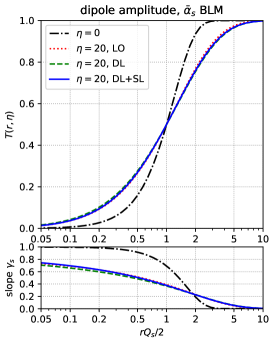
Figure 2: Top row: the dipole amplitude plotted as a function of the dimensionless quantity $rQ_{s}/2$. Bottom row: corresponding effective slope $\gamma_{s}=\partial\ln(T)/\partial\ln(r^{2})$. The 3 plots correspond to the same configurations as in Fig. 1.

Beside the saturation exponent which characterises the “speed” of the evolution, it is interesting to look at the form of the amplitude itself. Both the initial condition (dash-dotted black) and the amplitude at $\eta=20$ for different degrees of resummation (cf. Fig. 1) are shown in Fig. 2, for the same three configurations as in Fig. 1. Results are plotted as a function of the dimensionless ratio $rQ_{s}/2$ so as to better highlight the shape of the dipole amplitude. The bottom part of the plot shows the effective slope

$$\gamma_{s}(r,\eta)=\frac{\partial\ln(T(r,\eta))}{\partial\ln(r^{2})}.$$ (13)

Two striking features can be observed from these plots. First, the resummations of double and single transverse logarithms have a very small impact on the form of the amplitude. Even though a small effect is visible for the fixed-coupling evolution, almost no effect is observed with either running-coupling prescriptions. Then, one sees that the evolved amplitude has a less sharp transition between the dilute (small-$r$) and saturation (large-$r$) regions. This is particularly visible for the effective slope $\gamma_{s}$ which grows very slowly towards 1 at small dipole sizes.

4 Fits to the HERA data for inclusive DIS

We now come to our main task which is to describe the HERA data [46] for the inclusive DIS cross-section at $x\leq 0.01$.

4.1 The dipole factorisation and the fit set-up

The dipole factorisation for DIS at small $x$ (and at leading order in pQCD) expresses the physical picture in which the virtual photon fluctuates into a $q\bar{q}$ pair with a lifetime much longer than the longitudinal extent of the proton target. The total $\gamma^{*}p$ cross-section therefore factorises as a wavefunction for the $\gamma^{*}\to q\bar{q}$ splitting and an interaction between the dipole and the proton:

$$\sigma^{\gamma^{*}p}_{{\rm L},{\rm T}}(x,Q^{2})=\sum_{f}\int{\rm d}^{2}\bm{r}\int_{0}^{1}{\rm d}z\big{|}\Psi_{{\rm L},{\rm T}}^{(f)}(r,z;Q^{2})\big{|}^{2}\,\sigma_{\rm dipole}(\eta_{f},r),$$ (14)

where the squared light-cone wavefunctions (below, $\bar{Q}_{f}^{2}\equiv z(1-z)Q^{2}+m_{f}^{2}$)

$$\big{|}\Psi_{{\rm L}}^{(f)}(r,z;Q^{2})\big{|}^{2}=e_{q}^{2}\frac{\alpha_{\rm em}N_{c}}{2\pi^{2}}\,4Q^{2}z^{2}(1-z)^{2}{\rm K}_{0}^{2}\big{(}r\bar{Q}_{f}\big{)},$$ (15)

$$\big{|}\Psi_{{\rm T}}^{(f)}(r,z;Q^{2})\big{|}^{2}=e_{q}^{2}\frac{\alpha_{\rm em}N_{c}}{2\pi^{2}}\,\left\{\bar{Q}_{f}^{2}\left[z^{2}+(1-z)^{2}\right]{\rm K}_{1}^{2}\big{(}r\bar{Q}_{f}\big{)}+m_{f}^{2}{\rm K}_{0}^{2}\big{(}r\bar{Q}_{f}\big{)}\right\},$$ (16)

represent the probability that a (longitudinal or transverse) virtual photon splits into a $q\bar{q}$ colour dipole with transverse size $r$ and with “plus” longitudinal momentum fractions $z$ and $1-z$ for the quark and antiquark respectively. The sum in Eq. (14) runs over the quark flavors and our fit includes contributions from the three light quarks with $m_{u,d,s}=100$ MeV and from the charm quark, with $m_{c}=1.3$ GeV. Furthermore, $\sigma_{\rm dipole}(\eta_{f},r)$ is the dipole-proton total cross-section, evaluated for a proton (target) rapidity

$$\eta_{f}\equiv\ln\frac{1}{\tilde{x}_{f}}\quad\qquad\mbox{with}\qquad\tilde{x}_{f}\equiv x\big{(}1+4m_{f}^{2}/Q^{2}\big{)}\,.$$ (17)

In principle this cross-section should be computed by integrating the dipole scattering amplitude $T=1-S$ over all impact parameters, but since the impact-parameter dependence is non-perturbative and not properly encoded in the BK equation, we simply assume, in the spirit of a mean field picture, that the proton is a uniform disk of radius $R_{p}$ (treated as a fit parameter): $\sigma_{\rm dipole}(\eta_{f},r)=2\pi R_{p}^{2}T(\eta_{f},r)$, with $T(\eta,r)$ obtained from numerical solutions to the homogeneous version of Eq. (6).

One peculiar feature about Eq. (14) is the fact that the dipole cross-section is evaluated at the rapidity scale $\eta_{f}=\ln(1/\tilde{x}_{f})$, which refers to the virtual photon, and not to the dipole. This looks natural from the perspective of the target evolution in $k^{-}$ (recall the discussion following Eq. (1)), but it might look less obvious when thinking about the evolution of the dipole. Clearly, the dipole and the virtual photon have different rapidities, due to the splitting fraction $z$, which can be very asymmetric, i.e. $z\ll 1$ or $1-z\ll 1$, especially for a transverse photon . We show however in A that changes in the longitudinal and the transverse phase-spaces associated with the $\gamma^{*}\to q\bar{q}$ splitting compensate each other and that the use of the photon rapidity $\eta_{f}$ in (14) is valid.

The quantity we actually fit is the reduced cross-section, related to the $\gamma^{*}p$ cross-sections(14) by

$$\sigma_{\rm red} =\frac{Q^{2}}{4\pi^{2}\alpha_{\rm em}}\left[\sigma_{\rm T}^{\gamma^{*}p}+\frac{2(1-y)}{1+(1-y)^{2}}\sigma_{\rm L}^{\gamma^{*}p}\right].$$ (18)

$y$ is the inelasticity parameter defined through $Q^{2}=xys$, with $s$ the squared centre-of-mass energy of the $ep$ collision.

In order to solve the evolution equation (6), we still need to specify the running coupling prescription and the initial condition. For the running of the QCD coupling, we use the one-loop expression

$$\alpha_{s}(k_{\perp}^{2})=\frac{1}{b_{N_{\rm f}}\ln\big{(}k_{\perp}^{2}/\Lambda_{N_{\rm f}}^{2}\big{)}}\qquad\text{with }\qquad b_{N_{\rm f}}=\frac{11N_{c}-2N_{\rm f}}{12\pi},$$ (19)

where the dependence on the number of active flavours $N_{f}$ is made explicit. The value of $\Lambda_{5}$ is determined by imposing $\alpha_{s}(M_{Z}^{2})=0.1181$ [54], and $\Lambda_{3,4}$ are fixed by the continuity of $\alpha_{s}$ at the flavour thresholds. We use $m_{c}=1.3$ GeV and $m_{b}=4.5$ GeV for the charm and bottom quark masses. In coordinate space we use

$$\alpha_{s}(r)=\frac{1}{b_{N_{\rm f}}\ln\big{[}4C_{\alpha}^{2}/(r^{2}\Lambda_{N_{\rm f}}^{2})\big{]}},$$ (20)

where we included a fudge factor $C_{\alpha}$, which will be one of the parameters to be fitted to the data. Finally, we freeze $\alpha_{s}$ at a value $\alpha_{\rm sat}=1$ to regularise its infrared behaviour.

For the initial condition of the BK evolution, we use two parametrisations, most conveniently written for the dipole scattering amplitude $T(\eta,r)\equiv 1-S(\eta,r)$. The first choice corresponds to a modified version of the Golec-Biernat and Wüsthoff (GBW) “saturation model” [47] (used already in Fig. 1):

$${T}(\eta_{0},r)=\left\{1-\exp\left[-\left(\frac{r^{2}Q_{0}^{2}}{4}\right)^{p}\right]\right\}^{1/p},$$ (21)

where $Q_{0}$ and $p$ are parameters to be fitted. The parameter $p$, not present in the original GBW model, controls the shape of the amplitude close to saturation. Our second choice is a running-coupling version of the McLerran-Venugopalan (MV) model [49], called rcMV in the following, which reads:

$${T}(\eta_{0},r)=\left\{1-\exp\left[-\left(\frac{r^{2}Q_{0}^{2}}{4}\,\bar{\alpha}_{s}(r)\left[1+\ln\left(\frac{\bar{\alpha}_{\rm sat}}{\bar{\alpha}_{s}(r)}\right)\right]\right)^{p}\right]\right\}^{1/p}.$$ (22)

Once again, $Q_{0}$ and $p$ are free parameters (and $\alpha_{\rm sat}=1$). The other two parameters of the fit are $C_{\alpha}$ and $R_{p}$, the proton radius. In practice, we restrict $p$ and $C_{\alpha}$ to values smaller than 4 and 10, respectively. Indeed, the natural value for $p$ in the MV model is $p=1$ and it would be reassuring that the fits prefer such a value. Similarly, a natural value for $C_{\alpha}$ should be of order one.

4.2 Fit results

initial	RC	double	single	$\chi^{2}$ per	parameters
condition	scheme	logs	logs	data point	$R_{p}$[fm]	$Q_{0}$[GeV]	$C_{\alpha}$	$p$
		no	no	4.33	0.671	0.414	10	4
GBW	small	yes	no	2.05	0.786	0.355	10	4
		yes	yes	1.18	0.795	0.362	5.46	4
		no	no	1.88	0.764	0.374	10	4
GBW	BLM	yes	no	1.65	0.888	0.319	6.65	4
		yes	yes	1.14	0.762	0.377	0.788	4
		no	no	3.89	0.655	0.659	10	4
rcMV	small	yes	no	1.72	0.757	0.569	10	4
		yes	yes	1.03	0.772	0.561	5.66	1.76
		no	no	1.46	0.742	0.596	10	4
rcMV	BLM	yes	no	1.31	0.841	0.500	5.68	4
		yes	yes	1.01	0.758	0.503	0.897	1.01

Table 1: $\chi^{2}$ and values of the parameters fitted to HERA data.

In Table 1 we quote the results of the fit to the combined HERA data for the reduced cross section [46]. We include in the fit data points with $x<0.01$ and $Q^{2}<50$ GeV². For both initial conditions (GBW and rcMV) we show the results obtained using the two running coupling prescriptions (smallest dipole or BLM) in three cases corresponding to different resummations of transverse logarithms: pure LO (rcBK) evolution, resumming only double logarithms, or resumming both double and single logarithms.

One can see that the resummation of the double and of the single logarithms are both improving the agreement with the data. This is particularly the case for the resummation of single transverse logarithms which not only have a significant impact on the quality ($\chi^{2}$) of the fit, but also lead to more physical values for the fit parameters (in particular $C_{\alpha}$, for which values much larger than 1 mean that the evolution needs to be artificially slowed down by an unnaturally small value of the coupling in order to be compatible with data). These two resummations allow to reach values of $\chi^{2}$ per data point of less than 1.2 for all the combinations of initial conditions and running coupling prescriptions considered here. We believe (see e.g. the discussion in section 3) that this good agreement with the data is largely due to the reduction of the saturation exponent, $\lambda_{s}$, due to the resummation of transverse logs. A particular consequence is that, contrary to some previous rcBK fits, we do not need to use the peculiar Balitsky prescription for the running coupling [6] to obtain a good agreement with the data. One notices also that the fit shows a slight preference for the BLM running-coupling scheme which predicts slightly smaller saturation exponents compared to the smallest dipole prescription.

In Fig. 3 (left) we show the shape of the initial condition as a function of $r$ for the four fits which take into account the resummation of both single and double logarithms. The results look quite similar despite the different functional forms, which is due to the rather strong constraints from the data. In the right panel of Fig. 3, we show the saturation scale as a function of $x$ for each of these four fits, superimposed over the HERA data points that we use in the fit.

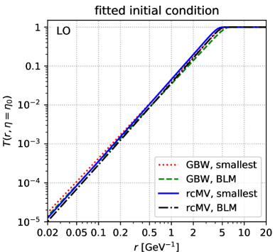
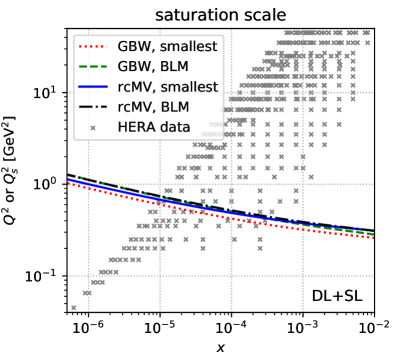
Figure 3: Left: initial conditions obtained from the fit as described in the text. Right: value of the saturation momentum, defined as $T(r=2/Q_{s}(\eta),\eta)=1/2$. The experimental data points from HERA [46] are shown for comparison.

In Table 2 we show how the fit is affected by including data with $Q^{2}$ larger than 50 GeV². A priori, one would not expect a very good agreement with data at such high transverse scales, where DGLAP effects are expected to be essential. Nevertheless one can see that, when including the single logarithms resummation, the fit quality remains about the same up to $Q^{2}_{\text{max}}=400$ GeV² for a rcMV initial condition. This is likely due to the fact that, as explained in section 2, these logarithms represent an important subset of the DGLAP contributions (at least at small $x$) and therefore improve the description at large $Q^{2}$. Even when resumming the single transverse logarithms, the fit quality gets worse when going to larger $Q^{2}$ with a GBW-type initial condition (21). This is probably related to the fact that the GBW model does not have the correct physical behaviour at large transverse momenta, or small dipole sizes.

initial	RC	double	single	$\chi^{2}$ per point vs. $Q^{2}_{\rm max}$
condition	scheme	logs	logs	50	100	200	400
		no	no	4.33	4.33	4.22	4.06
GBW	small	yes	no	2.05	2.17	2.27	2.24
		yes	yes	1.18	1.21	1.31	1.39
		no	no	1.88	1.93	2.04	2.07
GBW	BLM	yes	no	1.65	1.75	1.94	2.01
		yes	yes	1.14	1.17	1.25	1.32
		no	no	3.89	4.01	3.97	3.90
rcMV	small	yes	no	1.72	1.86	1.93	1.92
		yes	yes	1.03	1.04	1.01	1.00
		no	no	1.46	1.50	1.50	1.47
rcMV	BLM	yes	no	1.31	1.34	1.35	1.33
		yes	yes	1.01	1.03	1.01	1.00

Table 2: Evolution of the fit quality when increasing $Q^{2}_{\rm max}$ (in GeV²).

Since we take into account the charm contribution to the inclusive reduced cross section $\sigma_{\text{red}}$ in Eq. (18), we could also in principle compute the charm production cross section $\sigma_{\text{red}}^{c\bar{c}}$. In [43] it was found that, after fitting the data for the inclusive cross-section $\sigma_{\text{red}}$, a very good $\chi^{2}$/ndf ($<0.7$) was also obtained — without further tuning the fit parameters — for the $\sigma_{\text{red}}^{c\bar{c}}$ data presented in [55]. We believe that this was mostly a coincidence since a comparison between the best fits in [43] and the more recent, combined, HERA data for charm production [56], with more points and smaller uncertainties, shows a much worse agreement ($\chi^{2}/\text{ndf}>4$). The situation is similar with the present fit. This should not be a surprise as the inclusion of heavy flavour data in the saturation fits based on the BK equation is a longstanding issue. The resummations considered here are not expected to bring any concrete improvement on this issue, as they are not adapted to the inclusion of heavy quarks.

4.3 Positivity of the dipole amplitude’s Fourier transform

In this work we used the initial condition parametrisations (21) and (22) proposed in [43]. As was later shown [57], a drawback of these expressions is that their Fourier transforms are not positive-definite, which can lead to unphysical results in momentum space such as a negative unintegrated gluon distribution. The original GBW [47] and MV [49] parametrisations are not affected by this issue, however we were only able to obtain rather poor fits (with $\chi^{2}/\text{ndf}>1.4$) when using these expressions. A similar discussion applies to the more recent MV^e form, introduced in [53], which involves an extra parameter $e_{c}$ and reads

$$T(\eta_{0},r)=1-\exp\left[-\frac{r^{2}Q_{0}^{2}}{4}\ln\left(\frac{1}{r\Lambda}+e_{c}\cdot e\right)\right].$$ (23)

That said, it should be pointed out that the high-energy evolution tends to improve the situation. If we concentrate on our fits using the rcMV initial condition, which is physically most appealing, we numerically find that, even though the Fourier transform of the initial condition has negativity issues, the evolved amplitude becomes positive after a few units of rapidity, cf. Fig. 4 (left). (Some small oscillations remain in an intermediate rapidity range before disappearing at larger rapidities.) This happens because the solution develops an effective slope, defined in Eq. (13), which is smaller than 1 even for small $r$ as can be easily seen in the lower row in Fig. 2. This should be contrasted to the small-$r$ behaviour of the rcMV initial condition for $T(r)$, which vanishes faster than $r^{2}$ when $r\to 0$. In fact, after evolution, not only $S(r)$ but also $T(r)/r^{2}$ (whose Fourier transform is proportional to the gluon occupation number in the proton) satisfy all the conditions given in [57] which are necessary for a function to have a positive Fourier transform. This is confirmed by the numerical results displayed in Fig. 4.

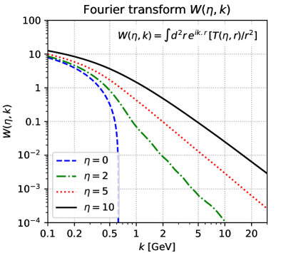
Figure 4: The Fourier transforms $S(\eta,k)\equiv\int{\rm d}^{2}\bm{r}\,{\rm e}^{{\rm i}\bm{k}\cdot\bm{r}}\,S(\eta,r)$ (left figure) and $W(\eta,k)\equiv\int{\rm d}^{2}\bm{r}\,{\rm e}^{{\rm i}\bm{k}\cdot\bm{r}}\,[T(\eta,r)/{r^{2}}]$ (right figure), as computed from numerical solutions to Eq. (6) with the rcMV initial condition and the BLM prescription for the RC. (The values of the free parameters are taken from the last line in Table 1.) The discontinuities in the curves corresponding to the initial condition ($\eta=0$) and the early rapidities reflect the negativity problem mentioned in Sect. 4.3.

Finding a functional form which has a positive-definite Fourier transform while preserving the good agreement with the HERA data would be extremely interesting, as this could open the way towards a unified description (via the dipole factorisation) of inclusive DIS and of particle production in “dilute-dense” ($ep$, $eA$, $pp$, $pA$) collisions. However, this seems to be also very challenging. At this level, it is legitimate to ask whether this difficulty solely reflects our inability to imagine versatile enough parametrisations for the initial condition, or it rather points towards a deeper problem with the dipole picture in the presence of a running coupling (perhaps similar to the problem discussed in [16] in the context of $pA$ collisions). However, addressing such deep issues goes well beyond the scope of the present work. Our main goal here was to show that, for a given and physically-motivated initial condition, the use of the collinearly-improved version of the BK evolution improves over the standard rcBK dynamics when it comes to a description of the HERA data for inclusive DIS at small $x$.

Appendix A On the rapidity phase-space for dipole evolution

Eq. (14) uses the rapidity argument $\eta\equiv\ln(1/x)=\ln(P^{-}/|q^{-}|)$ which is the logarithmic phase-space for the proton evolution down to the “minus” longitudinal momentum $|q^{-}|=Q^{2}/(2q^{+})$ of the virtual photon. This might seem odd since it makes explicit reference to the (longitudinal and transverse) kinematics of the virtual photon, and not to that of the dipole. One might expect that the dipole-proton scattering amplitude ${T}$ must be evolved over a smaller rapidity interval, since some of the longitudinal phase space is “consumed” to produce the splitting of the virtual photon into the $q\bar{q}$ pair. This issue is particularly important for a transverse photon, since the cross-section $\sigma_{\rm T}^{\gamma^{*}p}$ is dominated (at relatively high $Q^{2}$) by “aligned jet” configurations, such that $z$ is either very small, or very close to one. Moreover, it does not look natural that the dipole amplitude depends on $Q^{2}$ (via $\eta$); instead, it should depend on the dipole size $r^{2}$.

We argue here that the simultaneous changes in the longitudinal and the transverse phase-spaces associated with the $\gamma^{*}\to q\bar{q}$ splitting conspire to give a rapidity interval for the evolution of the dipole amplitude which is still equal to $\ln(1/x)$. We first observe that the difference $\hat{Y}$ in “projectile” rapidity between the dipole and the proton is fixed by the dipole leg with the smallest “plus” longitudinal momentum $\hat{q}^{+}=z_{\rm min}q^{+}$, with $z_{\rm min}\equiv{\rm min}(z,\,1-z)$; that is, $\hat{Y}=\ln(\hat{q}^{+}/q_{0}^{+})$, with $q_{0}^{+}=Q_{0}^{2}/2P^{-}$ as before (since this is fully a proton scale). The corresponding difference in the “target” rapidity is again obtained as $\hat{\eta}=\hat{Y}-\hat{\rho}$, with $\hat{\rho}=\ln(\hat{Q}^{2}/Q_{0}^{2})$ and $\hat{Q}^{2}=4/r^{2}$ the natural transverse resolution scale for the dipole. Hence,

$$\hat{\eta}=\hat{Y}-\hat{\rho}=\ln\frac{\hat{q}^{+}}{q_{0}^{+}}-\ln\frac{\hat{Q}^{2}}{Q_{0}^{2}}=\ln\frac{z_{\rm min}q^{+}P^{-}r^{2}}{2}=\ln\frac{1}{x}+\ln\frac{z_{\rm min}Q^{2}r^{2}}{4}\,.$$ (24)

We finally observe that (i) to the logarithmic accuracy of interest, we can approximate $z_{\rm min}\simeq z(1-z)$, and (ii) the integral in Eq. (14) is controlled by values of $r$ such that $4/r^{2}\sim z(1-z)Q^{2}$. Indeed, in the perturbative regime where $T\propto r^{2}$, the integral over $r$ “lives” at the largest possible values before it is eventually cut off by the exponential decrease of the modified Bessel functions (which exponentially vanish when their arguments become larger than one). This discussion implies $\hat{\eta}\simeq\eta$, as anticipated.

References

- [1] E. Iancu, K. Itakura, and L. McLerran, “Geometric scaling above the saturation scale,” Nucl. Phys. A708 (2002) 327–352, arXiv:hep-ph/0203137.
- [2] E. Iancu and R. Venugopalan, “The color glass condensate and high energy scattering in QCD,” arXiv:hep-ph/0303204.
- [3] F. Gelis, E. Iancu, J. Jalilian-Marian, and R. Venugopalan, “The Color Glass Condensate,” Ann.Rev.Nucl.Part.Sci. 60 (2010) 463–489, arXiv:1002.0333 [hep-ph].
- [4] T. Lappi, “Small x physics and RHIC data,” Int. J. Mod. Phys. E20 (2011) no. 1, 1–43, arXiv:1003.1852 [hep-ph].
- [5] Y. V. Kovchegov and E. Levin, Quantum chromodynamics at high energy. Cambridge University Press, 2012.
- [6] I. Balitsky, “Quark contribution to the small-x evolution of color dipole,” Phys.Rev. D75 (2007) 014001, arXiv:hep-ph/0609105 [hep-ph].
- [7] Y. V. Kovchegov and H. Weigert, “Triumvirate of Running Couplings in Small-x Evolution,” Nucl.Phys. A784 (2007) 188–226, arXiv:hep-ph/0609090 [hep-ph].
- [8] I. Balitsky and G. A. Chirilli, “Next-to-leading order evolution of color dipoles,” Phys.Rev. D77 (2008) 014019, arXiv:0710.4330 [hep-ph].
- [9] I. Balitsky and G. A. Chirilli, “Rapidity evolution of Wilson lines at the next-to-leading order,” Phys.Rev. D88 (2013) 111501, arXiv:1309.7644 [hep-ph].
- [10] A. Kovner, M. Lublinsky, and Y. Mulian, “Jalilian-Marian, Iancu, McLerran, Weigert, Leonidov, Kovner evolution at next to leading order,” Phys.Rev. D89 (2014) no. 6, 061704, arXiv:1310.0378 [hep-ph].
- [11] A. Kovner, M. Lublinsky, and Y. Mulian, “NLO JIMWLK evolution unabridged,” JHEP 08 (2014) 114, arXiv:1405.0418 [hep-ph].
- [12] M. Lublinsky and Y. Mulian, “High Energy QCD at NLO: from light-cone wave function to JIMWLK evolution,” JHEP 05 (2017) 097, arXiv:1610.03453 [hep-ph].
- [13] G. A. Chirilli, B.-W. Xiao, and F. Yuan, “One-loop Factorization for Inclusive Hadron Production in Collisions in the Saturation Formalism,” Phys. Rev. Lett. 108 (2012) 122301, arXiv:1112.1061 [hep-ph].
- [14] G. A. Chirilli, B.-W. Xiao, and F. Yuan, “Inclusive Hadron Productions in pA Collisions,” Phys. Rev. D86 (2012) 054005, arXiv:1203.6139 [hep-ph].
- [15] E. Iancu, A. H. Mueller, and D. N. Triantafyllopoulos, “CGC factorization for forward particle production in proton-nucleus collisions at next-to-leading order,” JHEP 12 (2016) 041, arXiv:1608.05293 [hep-ph].
- [16] B. Ducloué, E. Iancu, T. Lappi, A. H. Mueller, G. Soyez, D. N. Triantafyllopoulos, and Y. Zhu, “Use of a running coupling in the NLO calculation of forward hadron production,” Phys. Rev. D97 (2018) no. 5, 054020, arXiv:1712.07480 [hep-ph].
- [17] G. Beuf, “Dipole factorization for DIS at NLO I: Loop correction to the photon to quark-antiquark light-front wave-functions,” arXiv:1606.00777 [hep-ph].
- [18] G. Beuf, “Dipole factorization for DIS at NLO: Combining the and contributions,” Phys. Rev. D96 (2017) no. 7, 074033, arXiv:1708.06557 [hep-ph].
- [19] K. Roy and R. Venugopalan, “NLO impact factor for inclusive photondijet production in DIS at small ,” arXiv:1911.04530 [hep-ph].
- [20] I. Balitsky, “Operator expansion for high-energy scattering,” Nucl. Phys. B463 (1996) 99–160, arXiv:hep-ph/9509348.
- [21] J. Jalilian-Marian, A. Kovner, A. Leonidov, and H. Weigert, “The BFKL equation from the Wilson renormalization group,” Nucl. Phys. B504 (1997) 415–431, arXiv:hep-ph/9701284.
- [22] J. Jalilian-Marian, A. Kovner, A. Leonidov, and H. Weigert, “The Wilson renormalization group for low x physics: Towards the high density regime,” Phys.Rev. D59 (1998) 014014, arXiv:hep-ph/9706377 [hep-ph].
- [23] A. Kovner, J. G. Milhano, and H. Weigert, “Relating different approaches to nonlinear QCD evolution at finite gluon density,” Phys. Rev. D62 (2000) 114005, arXiv:hep-ph/0004014.
- [24] E. Iancu, A. Leonidov, and L. D. McLerran, “Nonlinear gluon evolution in the color glass condensate. I,” Nucl. Phys. A692 (2001) 583–645, arXiv:hep-ph/0011241.
- [25] E. Iancu, A. Leonidov, and L. D. McLerran, “The renormalization group equation for the color glass condensate,” Phys. Lett. B510 (2001) 133–144, arXiv:hep-ph/0102009.
- [26] E. Ferreiro, E. Iancu, A. Leonidov, and L. McLerran, “Nonlinear gluon evolution in the color glass condensate. II,” Nucl. Phys. A703 (2002) 489–538, arXiv:hep-ph/0109115.
- [27] Y. V. Kovchegov, “Small-x F2 structure function of a nucleus including multiple pomeron exchanges,” Phys. Rev. D60 (1999) 034008, arXiv:hep-ph/9901281.
- [28] J. L. Albacete, A. Dumitru, and C. Marquet, “The initial state of heavy-ion collisions,” Int.J.Mod.Phys. A28 (2013) 1340010, arXiv:1302.6433 [hep-ph].
- [29] T. Lappi and H. Mäntysaari, “Direct numerical solution of the coordinate space Balitsky-Kovchegov equation at next to leading order,” Phys.Rev. D91 (2015) no. 7, 074016, arXiv:1502.02400 [hep-ph].
- [30] E. Avsar, A. Stasto, D. Triantafyllopoulos, and D. Zaslavsky, “Next-to-leading and resummed BFKL evolution with saturation boundary,” JHEP 1110 (2011) 138, arXiv:1107.1252 [hep-ph].
- [31] G. Beuf, “Improving the kinematics for low-x QCD evolution equations in coordinate space,” Phys.Rev. D89 (2014) 074039, arXiv:1401.0313 [hep-ph].
- [32] J. Kwiecinski, A. D. Martin, and A. Stasto, “A Unified BFKL and GLAP description of F2 data,” Phys.Rev. D56 (1997) 3991–4006, arXiv:hep-ph/9703445 [hep-ph].
- [33] G. Salam, “A Resummation of large subleading corrections at small x,” JHEP 9807 (1998) 019, arXiv:hep-ph/9806482 [hep-ph].
- [34] M. Ciafaloni and D. Colferai, “The BFKL equation at next-to-leading level and beyond,” Phys.Lett. B452 (1999) 372–378, arXiv:hep-ph/9812366 [hep-ph].
- [35] M. Ciafaloni, D. Colferai, and G. Salam, “Renormalization group improved small x equation,” Phys.Rev. D60 (1999) 114036, arXiv:hep-ph/9905566 [hep-ph].
- [36] M. Ciafaloni, D. Colferai, G. Salam, and A. Stasto, “Renormalization group improved small x Green’s function,” Phys.Rev. D68 (2003) 114003, arXiv:hep-ph/0307188 [hep-ph].
- [37] A. Sabio Vera, “An ’All-poles’ approximation to collinear resummations in the Regge limit of perturbative QCD,” Nucl.Phys. B722 (2005) 65–80, arXiv:hep-ph/0505128 [hep-ph].
- [38] L. Lipatov, “Reggeization of the Vector Meson and the Vacuum Singularity in Nonabelian Gauge Theories,” Sov.J.Nucl.Phys. 23 (1976) 338–345.
- [39] E. Kuraev, L. Lipatov, and V. S. Fadin, “The Pomeranchuk Singularity in Nonabelian Gauge Theories,” Sov.Phys.JETP 45 (1977) 199–204.
- [40] I. Balitsky and L. Lipatov, “The Pomeranchuk Singularity in Quantum Chromodynamics,” Sov.J.Nucl.Phys. 28 (1978) 822–829.
- [41] E. Iancu, J. Madrigal, A. Mueller, G. Soyez, and D. Triantafyllopoulos, “Resumming double logarithms in the QCD evolution of color dipoles,” Phys.Lett. B744 (2015) 293–302, arXiv:1502.05642 [hep-ph].
- [42] T. Lappi and H. Mäntysaari, “Next-to-leading order Balitsky-Kovchegov equation with resummation,” Phys. Rev. D93 (2016) no. 9, 094004, arXiv:1601.06598 [hep-ph].
- [43] E. Iancu, J. D. Madrigal, A. H. Mueller, G. Soyez, and D. N. Triantafyllopoulos, “Collinearly-improved BK evolution meets the HERA data,” Phys. Lett. B750 (2015) 643–652, arXiv:1507.03651 [hep-ph].
- [44] J. L. Albacete, “Resummation of double collinear logs in BK evolution versus HERA data,” Nucl. Phys. A957 (2017) 71–84, arXiv:1507.07120 [hep-ph].
- [45] B. Ducloué, E. Iancu, A. H. Mueller, G. Soyez, and D. N. Triantafyllopoulos, “Non-linear evolution in QCD at high-energy beyond leading order,” JHEP 04 (2019) 081, arXiv:1902.06637 [hep-ph].
- [46] H1, ZEUS Collaboration, H. Abramowicz et al., “Combination of measurements of inclusive deep inelastic scattering cross sections and QCD analysis of HERA data,” Eur. Phys. J. C75 (2015) no. 12, 580, arXiv:1506.06042 [hep-ex].
- [47] K. J. Golec-Biernat and M. Wusthoff, “Saturation effects in deep inelastic scattering at low and its implications on diffraction,” Phys. Rev. D59 (1998) 014017, arXiv:hep-ph/9807513.
- [48] K. J. Golec-Biernat and M. Wusthoff, “Saturation in diffractive deep inelastic scattering,” Phys. Rev. D60 (1999) 114023, arXiv:hep-ph/9903358.
- [49] L. D. McLerran and R. Venugopalan, “Gluon distribution functions for very large nuclei at small transverse momentum,” Phys. Rev. D49 (1994) 3352–3355, arXiv:hep-ph/9311205.
- [50] J. L. Albacete, N. Armesto, J. G. Milhano, and C. A. Salgado, “Non-linear QCD meets data: A Global analysis of lepton-proton scattering with running coupling BK evolution,” Phys.Rev. D80 (2009) 034031, arXiv:0902.1112 [hep-ph].
- [51] J. L. Albacete, N. Armesto, J. G. Milhano, P. Quiroga-Arias, and C. A. Salgado, “AAMQS: A non-linear QCD analysis of new HERA data at small-x including heavy quarks,” Eur.Phys.J. C71 (2011) 1705, arXiv:1012.4408 [hep-ph].
- [52] J. Kuokkanen, K. Rummukainen, and H. Weigert, “HERA-Data in the Light of Small x Evolution with State of the Art NLO Input,” Nucl.Phys. A875 (2012) 29–93, arXiv:1108.1867 [hep-ph].
- [53] T. Lappi and H. Mäntysaari, “Single inclusive particle production at high energy from HERA data to proton-nucleus collisions,” Phys.Rev. D88 (2013) 114020, arXiv:1309.6963 [hep-ph].
- [54] Particle Data Group Collaboration, M. Tanabashi et al., “Review of Particle Physics,” Phys. Rev. D98 (2018) no. 3, 030001.
- [55] H1 Collaboration, F. Aaron et al., “Measurement of the Charm and Beauty Structure Functions using the H1 Vertex Detector at HERA,” Eur.Phys.J. C65 (2010) 89–109, arXiv:0907.2643 [hep-ex].
- [56] H1, ZEUS Collaboration, H. Abramowicz et al., “Combination and QCD analysis of charm and beauty production cross-section measurements in deep inelastic scattering at HERA,” Eur. Phys. J. C78 (2018) no. 6, 473, arXiv:1804.01019 [hep-ex].
- [57] B. G. Giraud and R. Peschanski, “Fourier-positivity constraints on QCD dipole models,” Phys. Lett. B760 (2016) 26–30, arXiv:1604.01932 [hep-ph].