Maxwell’s demon in a double quantum dot with continuous charge detection

Abstract

Converting information into work has during the last decade gained renewed interest as it gives insight into the relation between information theory and thermodynamics. Here we theoretically investigate an implementation of Maxwell’s demon in a double quantum dot and demonstrate how heat can be converted into work using only information. This is accomplished by continuously monitoring the charge state of the quantum dots and transferring electrons against a voltage bias using a feedback scheme. We investigate the electrical work produced by the demon and find a non-Gaussian work distribution. To illustrate the effect of a realistic charge detection scheme, we develop a model taking into account noise as well as a finite delay time, and show that an experimental realization is feasible with present day technology. Depending on the accuracy of the measurement, the system is operated as an implementation of Maxwell’s demon or a single-electron pump.

I Introduction

The conventional statement of the second law of thermodynamics is formulated for systems on the macroscopic scale and asserts that a change of entropy cannot be negative. It is therefore no surprise that it fails to describe systems that operate on a microscopic level. A feedback-controlled system that violates the conventional formulation of the second law was introduced by James C. Maxwell (Knott, 1911; Maxwell, 1871; Maruyama et al., 2009), who noted that a creature with the ability of tracking and determining the velocity of individual gas particles could create a temperature gradient. Scientists were confused by Maxwell’s demon for a long time, but following the work of Bennett Bennett (1982) and Landauer Landauer (1961), the process is completely legitimate. The demon acquires and stores information about the gas particles. Deleting this information requires an increase of entropy such that the second law is restored. These works established the close relationship between thermodynamics and information theory, suggesting that for feedback-controlled systems, the role of information must be incorporated into the formulation of the second law.

The field of stochastic thermodynamics deals with the microscopic nature of thermodynamics Bustamante et al. (2005); Seifert (2008, 2012); Horowitz and Gingrich (2020). It has revealed several important results, e.g. fluctuation theorems which generalize the second law to the nano-scale. During the course of the last decade, the incorporation of information in stochastic thermodynamics has resulted in a number of novel insights Leff and Rex (2002); Sagawa (2012); Maruyama et al. (2009); Parrondo et al. (2015); Potts and Samuelsson (2019a). In particular, fluctuation theorems have been generalized to hold for feedback-controlled systems Sagawa and Ueda (2008); Ponmurugan (2010); Sagawa and Ueda (2012a, b); Sourabh et al. (2012); Abreu and Seifert (2012); Potts and Samuelsson (2018) showing, in agreement with Bennett’s insight, that information can give rise to negative entropy production, and needs to be taken into account in the thermodynamic bookkeeping. Due to experimental advances, it is nowadays possible to control systems down to the nano-scale, making it possible to realize Maxwell’s demon in the lab. Several experimental studies have been conducted, using Brownian particles Toyabe et al. (2010), molecular machines Serreli et al. (2007), photonic systems Vidrighin et al. (2016), electronic systems Koski et al. (2014a, b); Chida et al. (2017); Koski et al. (2015), ultracold atoms Kumar et al. (2018), and DNA molecules Ribezzi-Crivellari and Ritort (2019). In addition, several experiments on Maxwell’s demon in the quantum regime have recently been presented Cottet et al. (2017); Masuyama et al. (2018); Naghiloo et al. (2018).

An advancement that is particularly promising for investigating the thermodynamics of information is provided by single electron charge detection in quantum dots Gustavsson et al. (2006); Lu et al. (2003); Fujisawa et al. (2004); Schleser et al. (2004); Vandersypen et al. (2004); Fujisawa et al. (2006). Detection of single electrons becomes highly important when realizing Maxwell’s demon in electronic circuits, where the electrons resemble the gas particles in the original thought experiment. Common charge detectors involve single electron transistors Lu et al. (2003); Fujisawa et al. (2004) and quantum point contacts (QPC) Schleser et al. (2004); Vandersypen et al. (2004). Such detectors are coupled capacitively to the electronic circuit under investigation. If the current through the detector depends sensitively on nearby charges, individual tunneling events of electrons can be resolved in real time. Experimental implementations of Maxwell’s demon based on charge sensing in single electron boxes are given in Refs. Koski et al. (2014a, b); Chida et al. (2017).

In this paper, we investigate an implementation of Maxwell’s demon in an electronic system constituted by two single-level quantum dots coupled to electron reservoirs at the same temperature. We theoretically demonstrate how heat can be converted into work by transferring electrons against an external voltage bias using a measurement and feedback scheme. During the process, the electron occupation of the dots is measured, and this information is used to guide the electrons through the system by tuning the energy level positions of the dots. We provide a quantitative statistical analysis of the electron transport by employing full counting statistics (FCS). From the FCS, the statistics of work and heat can directly be extracted. We first consider an ideal detector providing perfect knowledge on the charge state at each moment in time. Then we investigate a realistic detector where both delay and noise are taken into account.

An analogous operation cycle was first presented by Averin, Möttönen, and Pekola in Ref. Averin et al. (2011) for a system constituted by metallic islands. In this paper, we go beyond their results by considering a complete statistical study on the electron transport, and an implementation of a realistic detector model. Furthermore, in contrast to Refs. Koski et al. (2014a, b); Averin et al. (2011), our implementation is based on quantum dots, offering the possibility of tuning electron tunneling rates. Furthermore, the well defined energy levels of quantum dots allow for accessing heat fluctuations. We note that it is easy to establish a large inter-dot Coulomb blockade in the double dot system which may provide a challenge in metallic islands.

Previously proposed implementations of Maxwell’s demon based on charge sensing in a single quantum dot have been presented in Refs. Schaller et al. (2011, 2018), where electrons are transferred against a voltage bias by tuning electron tunneling rates. Another class of implementations are autonomous Maxwell demons, which do not rely on an external measurement and feedback loop. Several theoretical Strasberg et al. (2013); Kutvonen et al. (2016); Strasberg et al. (2018); Erdman et al. (2018); Sánchez et al. (2019) as well as experimental Koski et al. (2015) studies making use of autonomous charge sensing have been presented.

The paper is organized as follows. In Sec. II, the double quantum dot system is introduced together with a description of the ideal operation cycle. Section III is devoted to the results obtained when operating the system ideally, while Sec. IV presents the results for a realistic detector.

II System and ideal operation

By confining electrons in a small volume, for instance in a nanowire, it is possible to define an atomlike structure that is known as a quantum dot. By monitoring the charge states of these structures, and modifying their internal properties, it is possible to implement Maxwell’s demon. Here, we consider two quantum dots coupled in series to each other with tunneling rate $\gamma$, and to an equilibrium electron reservoir each with tunneling rates $\Gamma_{L}$ and $\Gamma_{R}$, respectively. The reservoirs $L$ and $R$ are described by the Fermi-Dirac distribution

$$f_{L/R}(\epsilon)=\big{[}e^{(\epsilon-\mu_{L/R})/k_{B}T}+1\big{]}^{-1},$$ (1)

where $\epsilon$ denotes energy, $T$ the temperature, and $\mu_{L/R}$ the chemical potential. We assume large intra- and inter-dot Coulomb repulsion such that only one electron can reside in the double quantum dot, and we neglect degeneracies (e.g. spin). Finally, we assume that the coherence time is shorter than any other relevant time-scale such that superpositions of charge states can be neglected. This implies that the system can be in one of three distinct states: $(0,0)$, $(1,0)$, and $(0,1)$, corresponding to empty dots, left dot occupied, and right dot occupied, respectively. We assume that the energy levels of the dots, denoted by $\{\epsilon_{L},\epsilon_{R}\}$, can be tuned by external voltage gates. We restrict ourselves to the three level settings: $\{\epsilon_{0},\epsilon_{u}\}$, $\{\epsilon_{l},\epsilon_{l}\}$, and $\{\epsilon_{u},\epsilon_{0}\}$, illustrated in Fig. 1.

Our aim is to show that electrons can be moved against an external voltage bias $\mu_{R}-\mu_{L}=eV$ without performing work by the voltage gates. This is achieved by measuring the occupation of the dots and applying feedback. The operation we consider is illustrated in Fig. 1 and shows how the electrons are transferred against the bias using information alone. In this and the next section, we consider ideal operation conditions. This corresponds to three assumptions. First, we assume that the continuous occupation measurements of the dots are error-free such that we know the system state with certainty at all times. Second, it is assumed that the feedback is applied instantaneously. Finally, we choose $\mu_{L/R}-\epsilon_{l}\gg k_{B}T$ and $\epsilon_{u}-\mu_{L/R}\gg k_{B}T$ such that the occupation probabilities for $\epsilon_{l}$ and $\epsilon_{u}$ can be approximated as $f_{L/R}(\epsilon_{l})=1$ and $f_{L/R}(\epsilon_{u})=0$. In Sec. IV, we will consider a non-ideal demon, where the first and third assumptions will be relaxed. Letting $\mu_{L}<\mu_{R}$, the following cyclic scheme can be utilized:

1. Initially, the dots are empty, and the energy levels are set to $\{\epsilon_{0},\epsilon_{u}\}$, as visualized in , see Fig. 1. With these settings, the only event possible is an electron tunneling into the left dot. When this occurs, the levels are immediately moved to $\{\epsilon_{l},\epsilon_{l}\}$, see , such that the electron cannot tunnel back to the left reservoir.

2. As the electron tunnels to the right dot, the energy levels are moved instantly to $\{\epsilon_{u},\epsilon_{0}\}$, as depicted in .

3. The electron can now only tunnel to the right reservoir. As this happens, the levels are moved back to their initial position in , closing the cycle.

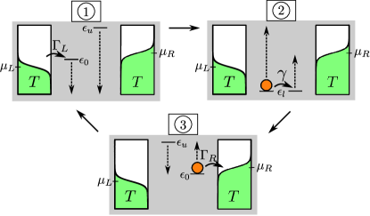
Figure 1: Visualization of the demon cycle. Curved arrows depict possible electron tunneling events, where $\Gamma_{L}$, $\Gamma_{R}$, and $\gamma$ are electron tunneling rates. As soon as such an event occurs, it is immediately detected and the energy levels are moved as illustrated by the dashed arrows.

For each cycle, the first law of thermodynamics can be written as $Q+W+W_{g}=0$. The work $W=\mu_{R}-\mu_{L}=eV$ is performed by moving one electron from a region with lower to a region with higher chemical potential. The corresponding heat $Q_{L}=\mu_{L}-\epsilon_{0}$ and $Q_{R}=\epsilon_{0}-\mu_{R}$ enters the left and right reservoirs, cooling both reservoirs when $\mu_{L}<\epsilon_{0}<\mu_{R}$. The total heat is given by $Q=Q_{L}+Q_{R}=-W$. The total work extracted by the gates $W_{g}=(\epsilon_{0}-\epsilon_{l})+(\epsilon_{l}-\epsilon_{0})=0$ vanishes, as desired. Finally, the change in system energy is zero as the process is cyclic. Here, we use the convention $Q>0$ if energy is entering a reservoir, and $W>0$ when work is produced. Thus, for $eV\geq 0$, heat is converted into work using information.

III Ideal demon: Quantitative description

Under ideal conditions, the occupation of the quantum dots uniquely determines the level positions $\{\epsilon_{L},\epsilon_{R}\}$. Hence, the system dynamics can be described by the rate equation $\boldsymbol{\dot{\rho}}_{0}(t)=\mathcal{L}_{0}\boldsymbol{\rho}_{0}(t)$, where the components $\rho_{0,j}(t)$, $j=(0,0)$, $(1,0)$, $(0,1)$, of $\boldsymbol{\rho}_{0}(t)$ are the probabilities to occupy state $j$ at time $t$. The Liouvillian $\mathcal{L}_{0}$ and the transition rates between the system states are determined by the following transitions representing the ideal cycle

$$(0,0)\xrightarrow{\makebox[8.5359pt]{$\gamma_{L}$}}(1,0)\xrightarrow{\makebox[8.5359pt]{$\gamma$}}(0,1)\xrightarrow{\makebox[8.5359pt]{$\gamma_{R}$}}(0,0),$$ (2)

where

$$\gamma_{L}=\Gamma_{L}f_{L}(\epsilon_{0}),\hskip 28.45274pt\gamma_{R}=\Gamma_{R}\left[1-f_{R}(\epsilon_{0})\right],$$ (3)

see Fig. 1.

III.1 Full counting statistics

To describe the statistics of the electron transport in the system, we use FCS (Levitov et al., 1996), the central object of which is given by the probability distribution of the number of electrons transferred to the right reservoir within the time $t$, $p(n,t)=\sum_{j}\rho_{j}(n,t)$, with $\rho_{j}(n,t)$ being the components of the number-resolved probability vector $\boldsymbol{\rho}(n,t)$. With the discrete Fourier transform of $\boldsymbol{\rho}(n,t)$ given by $\boldsymbol{\rho}(\chi,t)$ where the counting field $\chi$ is introduced, the dynamics of the system is governed by the differential equation Schaller (2014)

$$\dot{\boldsymbol{\rho}}(\chi,t)=\mathcal{L}(\chi)\boldsymbol{\rho}(\chi,t),$$ (4)

with the Liouvillian

$$\mathcal{L}(\chi)=\begin{pmatrix}-\gamma_{L}&0&e^{i\chi}\gamma_{R}\\ \gamma_{L}&-\gamma&0\\ 0&\gamma&-\gamma_{R}\end{pmatrix}.$$ (5)

By putting $\chi=0$, the rate equation in Eq. (2) is recovered, i.e. $\mathcal{L}_{0}=\mathcal{L}(0)$.

The cumulant generating function (CGF) $\mathcal{C}(\chi,t)$ of the probability distribution is defined via

$$e^{\mathcal{C}(\chi,t)}=\sum_{n}p(n,t)e^{in\chi}=\sum_{j}\rho_{j}(\chi,t),$$ (6)

and the cumulants are obtained using

$$\langle\!\langle n^{k}(t)\rangle\!\rangle=(-i)^{k}\left.\frac{\partial^{k}}{\partial\chi^{k}}\mathcal{C}(\chi,t)\right|_{\chi=0}.$$ (7)

In the long time-limit, the CGF is given, up to a time independent correction term which will be dropped in the following, by $\mathcal{C}(\chi,t)\approx\lambda(\chi)t$, where $\lambda(\chi)$ is the eigenvalue of the Liouvillian that satisfies $\lambda(0)=0$ Schaller (2014). The eigenvalue is given by one of the roots of the characteristic polynomial of $\mathcal{L}(\chi)$

$$\lambda^{3}+(\gamma+\gamma_{L}+\gamma_{R})\lambda^{2}+( \gamma\gamma_{L}+\gamma\gamma_{R}+\gamma_{L}\gamma_{R})\lambda$$ (8)

$$+\gamma\gamma_{L}\gamma_{R}(1-e^{i\chi})=0.$$

The solutions of this equation do not provide additional physical insight, and are therefore not given here. Note that Eq. (8) is invariant under the exchange of any two transition rates, implying that also the cumulants possess this symmetry. The first, second, and third order cumulants are given by

$$\langle\!\langle n(t)\rangle\!\rangle =\frac{\gamma\gamma_{L}\gamma_{R}}{\gamma\gamma_{L}\!+\!\gamma\gamma_{R}\!+\!\gamma_{L}\gamma_{R}}t,$$ (9)

$$\langle\!\langle n^{2}(t)\rangle\!\rangle =\langle\!\langle n(t)\rangle\!\rangle\frac{\gamma^{2}\gamma_{L}^{2}+\gamma^{2}\gamma_{R}^{2}+\gamma_{L}^{2}\gamma_{R}^{2}}{\left(\gamma\gamma_{L}+\gamma\gamma_{R}+\gamma_{L}\gamma_{R}\right)^{2}},$$

$$\langle\!\langle n^{3}(t)\rangle\!\rangle =\langle\!\langle n(t)\rangle\!\rangle\left[1-\frac{6\langle\!\langle n(t)\rangle\!\rangle}{\gamma\gamma_{L}\gamma_{R}t}\right.$$

$$\times\left.\left(\frac{\langle\!\langle n(t)\rangle\!\rangle^{2}}{t^{2}}-(\gamma\!+\!\gamma_{L}\!+\!\gamma_{R})\frac{\langle\!\langle n^{2}(t)\rangle\!\rangle}{t}\right)\right].$$

Finally, the full distribution is obtained through

$$p(n,t)=\frac{1}{2\pi}\int^{2\pi}_{0}d\chi e^{-in\chi+\lambda(\chi)t}.$$ (10)

III.2 Power production

We are interested in the electrical power $P=V\cdot I$ which is a measure of the heat-to-work conversion resulting from the demon operation. Note that a positive current here is defined to flow against the bias. The power is related to the produced work via $W=\int Pdt$. The low frequency power cumulants for the system studied here are given by

$$\langle\!\langle P^{k}\rangle\!\rangle=(eV)^{k}\lim_{t\rightarrow\infty}\frac{\langle\!\langle n^{k}(t)\rangle\!\rangle}{t}.$$ (11)

We start by considering the mean power

$$\frac{\langle\!\langle P\rangle\!\rangle}{\gamma k_{B}T}=\frac{eV}{k_{B}T}\frac{\gamma_{L}\gamma_{R}}{\gamma\gamma_{L}+\gamma\gamma_{R}+\gamma_{L}\gamma_{R}},$$ (12)

that is plotted in Fig. 2 as a function of $\epsilon_{0}$ (cf. Fig. 1) and the voltage bias $eV$. The plots show that $\langle\!\langle P\rangle\!\rangle\geq 0$ for all parameters which is due to the ideal operation conditions ensuring that electrons are only transferred from left to right. This demonstrates that information can be used to convert heat into work in this system. From Eq. (12), it is clear that the power increases with increasing tunneling rates. For fixed tunneling rates, $\Gamma_{L}$, $\Gamma_{R}$, $\gamma$, the power attains its largest value at

$$\frac{\epsilon_{0}}{k_{B}T} =\frac{1}{2}\ln\left[\frac{\Gamma_{L}}{\Gamma_{R}}\right],$$ (13a)

$$\frac{eV}{k_{B}T} =2\left[W\left(\frac{\Gamma_{L}+\Gamma_{R}+\Gamma_{L}\Gamma_{R}/\gamma}{2e\sqrt{\Gamma_{L}\Gamma_{R}}}\right)+1\right],$$ (13b)

where $W(z)$ is the Lambert W-function Corless et al. (1996), also known as the product logarithm function. Note that $e$ on the right hand side of Eq. (13b) is Euler’s number and not the elementary charge. For $\Gamma_{L}=\Gamma_{R}$, the maximum is located at $\epsilon_{0}=0$, i.e. in the middle of the bias window. For $\Gamma_{L}\neq\Gamma_{R}$, this is no longer true; compare Figs. 2(a) and (b).

Another feature in Fig. 2(a), where $\Gamma_{L}=\Gamma_{R}$, is the mirror symmetry around $\epsilon_{0}=0$. This corresponds to the transformation $\gamma_{L}\leftrightarrow\gamma_{R}$, which is the exchange-symmetry of transition rates in the charactersitic polynomial discussed above. In Fig. 2(b), where $\Gamma_{L}\neq\Gamma_{R}$, the transformation $\gamma_{L}\leftrightarrow\gamma_{R}$ has a more complicated effect.

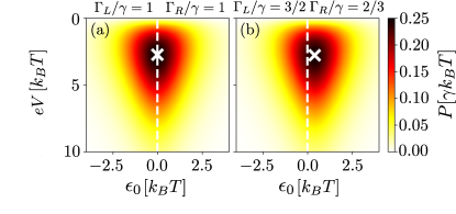
Figure 2: First order power cumulant $\langle\!\langle P\rangle\!\rangle$ in units of $\gamma k_{B}T$ as a function of $\epsilon_{0}$ and the voltage bias $eV$ for tunneling rates (a) $\Gamma_{L}/\gamma=\Gamma_{R}/\gamma=1$, and (b) $\Gamma_{L}/\gamma=3/2$, $\Gamma_{R}/\gamma=2/3$. The white, dashed line emphasizes where $\epsilon_{0}=0$, and the white cross indicates where the power reaches its maximum. Here, the chemical potentials are chosen as $\mu_{R}=eV/2=-\mu_{L}$ which is not necessarily symmetric around $\epsilon_{0}$. For non-equal tunneling rates, a symmetric bias around $\epsilon_{0}$ is no longer optimal.

III.3 Fano factor and skewness

The Fano factor is defined as the ratio between the second and first order cumulants [cf. Eq. (7)], and gives a measure on the statistical character of the electron transport. For a Poisson process, the Fano factor is 1. A smaller Fano factor implies sub-, a larger super-Poissonian statistics corresponding to anti-bunching Wagner et al. (2017) and bunching Maisi et al. (2014, 2016); Fujita et al. (2016) of electrons, respectively.

With the first and second order cumulants given by Eqs. (9), the Fano factor reads,

$$\frac{1}{eV}\frac{\langle\!\langle P^{2}\rangle\!\rangle}{\langle\!\langle P\rangle\!\rangle}=\frac{\langle\!\langle n^{2}(t)\rangle\!\rangle}{\langle\!\langle n(t)\rangle\!\rangle}=\frac{\gamma^{2}\gamma_{L}^{2}+\gamma^{2}\gamma_{R}^{2}+\gamma_{L}^{2}\gamma_{R}^{2}}{\left(\gamma\gamma_{L}+\gamma\gamma_{R}+\gamma_{L}\gamma_{R}\right)^{2}}.$$ (14)

The Fano factor is visualized in Fig. 3(a) as a function of the weighted transition rates $\gamma_{L}/\gamma$ and $\gamma_{R}/\gamma$. The symmetry of exchanging $\gamma_{L}$ and $\gamma_{R}$ discussed above is evident in the figure. In our system, we find the Fano factor to be bounded by

$$\frac{1}{3}\leq\frac{\langle\!\langle n^{2}(t)\rangle\!\rangle}{\langle\!\langle n(t)\rangle\!\rangle}\leq 1,$$ (15)

where the lower bound corresponds to having all transition rates equal. A Fano factor smaller than one is expected since only a single electron can occupy the system at a time resulting in anti-bunching. The upper bound occurs when any of the transition rates is much smaller than the other two, e.g. when $\gamma\ll\gamma_{L},\gamma_{R}$. In this regime, the system behaves effectively as a single tunneling barrier and the statistics are Poissonian.

Figure 3(b) visualizes the normalized third order cumulant $\langle\!\langle n^{3}(t)\rangle\!\rangle/\langle\!\langle n(t)\rangle\!\rangle$ which captures the skewness of the distribution $p(n,t)$. Since the third order cumulant is non-zero, the transport statistics, and therefore also the heat and work statistics, are non-Gaussian.

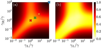
Figure 3: (a) Fano factor $\langle\!\langle n^{2}(t)\rangle\!\rangle/\langle\!\langle n(t)\rangle\!\rangle$ as function of $\gamma_{L}/\gamma$ and $\gamma_{R}/\gamma$. The Fano factor is bounded from above by 1, and from below by 1/3. The upper bound is obtained when one transition rate is much smaller than the others, corresponding to the dark areas in the corners. The lower bound is obtained when all transition rates are equal, corresponding to the bright area in the middle. The colored crosses visualize the choice of parameters in Fig. 4. (b) Normalized third order cumulant $\langle\!\langle n^{3}(t)\rangle\!\rangle/\langle\!\langle n(t)\rangle\!\rangle$. This factor only assumes finite values implying non-Gaussian statistics for work and heat.

III.4 Probability distributions

The full distribution $p(n,t)$, which is directly related to the work and heat distributions by $W=neV$ and $Q=-W$, can be evaluated in the long time limit using Eq. (10). It is instructive to consider two limiting cases. First, when one transition rate is much smaller than the others, e.g. $\gamma\ll\gamma_{L},\gamma_{R}$, we may expand the dominant eigenvalue of the Liouvillian up to linear order in $\gamma$, obtaining $\lambda(\chi)=\gamma\left(e^{i\chi}-1\right)$. With Eq. (10), this results in

$$p(n,t)=e^{-\gamma t}\frac{(\gamma t)^{n}}{n!},$$ (16)

which is the Poisson distribution, in agreement with the discussion on the Fano factor above.

Second, with all transition rates equal, $\gamma=\gamma_{L}=\gamma_{R}$, the total number of tunneling events $q$ in the system is distributed according to Eq. (16). Starting in the state $(0,0)$, an electron must tunnel three times before reaching the right reservoir, see Fig. 1. To have $n$ electrons transferred to the right reservoir, $q=3n+k$ tunneling events must have occured, with $k=0,1,2$. This results in the distribution

$$p(n,t)=e^{-\gamma t}\sum_{k=0,1,2}\frac{(\gamma t)^{3n+k}}{(3n+k)!}.$$ (17)

Equations (16) and (17) are visualized in Fig. 4 together with the distributions for $(\gamma_{L}/\gamma,\gamma_{R}/\gamma)=(3,2)$ and $(\gamma_{L}/\gamma,\gamma_{R}/\gamma)=(8,5)$, calculated numerically. The center of each distribution, i.e. the mean, agrees with the first order cumulant in Eq. (9). As the third order cumulant in Eq. (9) is non-zero and positive [see Fig. 3(b)], the distribution always has a skewness, and is therefore non-Gaussian. The direct relation between $p(n,t)$ and the distributions of work and heat reveals the non-Gaussian statistics of these thermodynamic quantities.

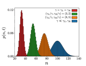
Figure 4: Probability distribution $p(n,t)$ in four cases as a function of $n$ for $\gamma t=100$. The red and blue bars represent the analytical solutions obtained when all transition rates are equal and when one rate is much smaller than the others, respectively [see Eqs. (16) and (17)]. The green and orange bars were obtained numerically.

III.5 Entropy production of the demon

The operation described in Sec. II results in an entropy reduction in the system. It is therefore required that the entropy produced by the demon balances this reduction such that the system and demon together obeys the second law of thermodynamics. Recently, bounds on entropy production in heat engines have been derived within the framework of thermodynamic uncertainty relations (TURs) Gingrich et al. (2016); Potts and Samuelsson (2019b); Horowitz and Gingrich (2020); Van Vu and Hasegawa (2020). To derive a TUR for our system and demon is a daunting task, and is not attempted here. However, by assuming that a generic TUR holds, derived for a number of different systems, we can establish a lower bound for the entropy production. The TUR considered is given by

$$\frac{\langle\!\langle I^{2}\rangle\!\rangle}{\langle\!\langle I\rangle\!\rangle^{2}}\geq\frac{2}{\sigma_{S}+\sigma_{D}},$$ (18)

where $\langle\!\langle I\rangle\!\rangle$ and $\langle\!\langle I^{2}\rangle\!\rangle$ are the two lowest order current cumulants obtained from $\langle\!\langle I^{k}\rangle\!\rangle=\lim_{t\rightarrow\infty}e^{k}\langle\!\langle n^{k}(t)\rangle\!\rangle/t$ with the elementary charge $e$, and $\sigma_{S}$ and $\sigma_{D}$ are the entropy production (in units of $k_{B}$) for the system and demon, respectively. The entropy production for the system is obtained through $\sigma_{S}=-\langle\!\langle I\rangle\!\rangle V/k_{B}T$, which is the heat current into the reservoirs divided by their temperature $T$. For the demon entropy production, we may write $\sigma_{D}=x_{D}\langle\!\langle I\rangle\!\rangle/k_{B}T$, where $x_{D}$ is the entropy production in the demon in units of $-\sigma_{S}$. The total entropy production for the system and demon together can then be written as

$$\sigma_{S}+\sigma_{D}=\frac{\langle\!\langle I\rangle\!\rangle}{k_{B}T}\left(x_{D}-1\right).$$ (19)

Using this together with the TUR given in Eq. (18), the following inequality for $x_{D}$ can be obtained,

$$x_{D}\geq 1+\frac{2k_{B}T}{eV}\frac{1}{F},$$ (20)

where $F$ is the Fano factor in Eq. (14). This sets a lower bound on the demon entropy production. As $x_{D}\geq 1$, it is assured that the total entropy production $\sigma_{S}+\sigma_{D}\geq 0$, and thus the second law is respected.

It is instructive to introduce the efficiency

$$\eta\equiv\frac{-\sigma_{S}}{\sigma_{D}}=\frac{1}{x_{D}}\leq\frac{eV\cdot F}{eV\cdot F+2k_{B}T},$$ (21)

which relates the entropy reduction in the system to the entropy produced by the demon. In the reversible limit, where the demon produces the minimal amount of entropy allowed by the second law, the efficiency is maximal and equal to unity. From Eq. (21), we find that the reversible limit may only be reached for $eV\gg k_{B}T$.

IV Non-ideal demon

So far, we have focused on ideal operation conditions relying on an ideal detector that is infinitely fast and error free. Here we consider a more realistic model describing a QPC or quantum dot detector asymmetrically coupled to the double dot system Fujisawa et al. (2006); Küng et al. (2012). In particular, we include delay as well as noise in the charge sensing. These constitute the main error sources in realistic detectors. Furthermore, we relax the requirement that $f_{L/R}[\epsilon_{u(l)}]=0(1)$ for a more realistic description. We note that we still consider the change of the energy levels to happen on a time-scale that is much faster than any other relevant time-scale. This is experimentally feasible Pothier et al. (1992); Küng et al. (2012); Koski et al. (2014a, b).

IV.1 Model

We start by providing a general formulation of the model for the detector, its output, and the feedback. The system state after time $t$ is denoted by $S(t)$, and assumes the values 0, 1, and 2 representing the charge configurations $(0,0)$, $(1,0)$, and $(0,1)$, respectively. For the detector, we introduce a detector output $d(t)$ which is dependent on the system state $S(t)$, a delay time $\tau_{d}$, and assume that the detector adds Gaussian white noise with standard deviation $\sigma$ on its output. The energy level setting after time $t$ is described by $D(t)$, also taking the values 0, 1, and 2, but here representing the settings $\{\epsilon_{0},\epsilon_{u}\}$, $\{\epsilon_{l},\epsilon_{l}\}$, and $\{\epsilon_{u},\epsilon_{0}\}$, respectively.

The system state $S(t)$ is a stochastic variable whose trajectory is determined by the probability vector $\boldsymbol{\rho}(t)$ that is governed by the rate equation

$$\boldsymbol{\dot{\rho}}(t)=\mathcal{L}\left[D(t)\right]\boldsymbol{\rho}(t),$$ (22)

where the Liouvillaian $\mathcal{L}\left[D(t)\right]$ is dependent on the current energy level setting. The Liouvillian is given in Appendix A. $D(t)$ is governed by a measurement-feedback scheme which depends on the detector output $d(t)$. We model the detector output as a random Gaussian variable distributed as

$$p\left[d(t)\right]=\frac{1}{\sqrt{2\pi\sigma^{2}}}e^{-\left[d(t)-m(t)\right]^{2}/2\sigma^{2}},$$ (23)

with the standard deviation $\sigma$ quantifying the strength of the noise. The mean of the distribution is given by

$$m(t)=\int_{-\infty}^{t}\tau_{d}^{-1}e^{-(t-t^{\prime})/\tau_{d}}S(t^{\prime})dt^{\prime},$$ (24)

where the delay $\tau_{d}$ is introduced. The insets of Fig. 5 visualize $d(t)$ for some different choices of $\tau_{d}$ and $\sigma$. With the dots unoccupied, $d(t)$ is distributed around 0, and with one of the dots occupied, the signal is distributed around 1 or 2 depending on the location of the electron. The rise time of the signal is determined by $\tau_{d}$. The ideal limit corresponds to $\tau_{d}$, $\sigma\rightarrow 0$, where we find $d(t)=S(t)$ at all times. Having a model for the detector output, we need to provide a feedback protocol, determining the level setting $D(t)$ from the previous output $d(t^{\prime}\leq t)$. This is provided by

$$D(t)=\operatorname*{arg\hskip 2.27621ptmax}_{j\in\{0,1,2\}}\int_{t-4\tau_{d}}^{t}dt^{\prime}\theta_{j}\left[d(t^{\prime})\right],$$ (25)

with $\theta_{0}[x]=\Theta\left[\frac{1}{2}-x\right]$, $\theta_{1}[x]=\Theta\left[x-\frac{1}{2}\right]\Theta\left[\frac{3}{2}-x\right]$, and $\theta_{2}[x]=\Theta[x-\frac{3}{2}]$, where $\Theta[x]$ is the Heaviside step function. Equation (25) works as follows; if $d(t^{\prime})<\frac{1}{2}$ in the majority of the interval $[t-4\tau_{d},t]$, below referred to as checking interval, the charge configuration is assumed to be $(0,0)$, i.e. $S(t)=0$, and the level setting is put to $D(t)=0$. When $\frac{1}{2}\leq d(t^{\prime})<\frac{3}{2}$ in the majority of the checking interval, the system is assumed to occupy $S(t)=1$, and the level setting $D(t)=1$ is chosen. Finally, as $d(t^{\prime})\geq\frac{3}{2}$ in the majority of the checking interval, the level setting is put to $D(t)=2$. In contrast to standard threshold detection Küng et al. (2012); Koski et al. (2013), the use of a checking interval reduces the risk of misinterpreting transitions. For instance, this ensures that the level position setting does not pass through $\{\epsilon_{l},\epsilon_{l}\}$ ($D(t)=1$) when $d(t^{\prime})$ changes from 2 to 0 in a short time. For $\tau_{d}\rightarrow 0$, the checking interval becomes infinitely small, and $D(t)$ is determined by the instantaneous value of $d(t)$, leading to $D(t)=d(t)=S(t)$ in the ideal limit, where $\sigma\rightarrow 0$. The feedback is thus infinitely fast in the ideal limit, and we recover the results of the previous section.

IV.2 Monte Carlo simulations

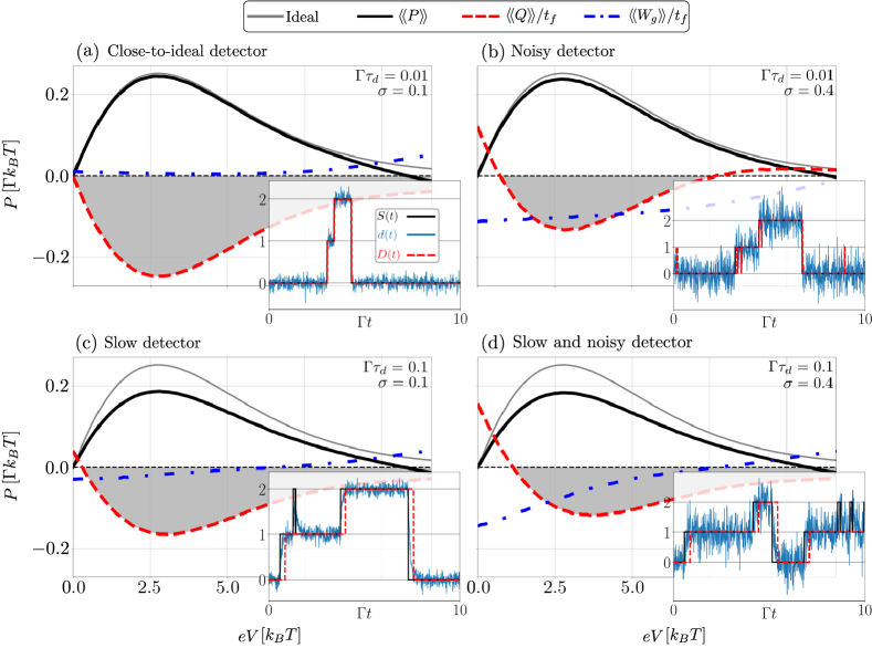
Figure 5: Energy fluxes as functions of the voltage bias. (a)-(d) visualize the effect of different choices for $\tau_{d}$ and $\sigma$. In the gray, shaded regions, the heat is negative, seemingly violating the second law, and the system is operated as a Maxwell demon. The insets show examples of time traces of the true system state $S(t)$, the detector output $d(t)$, and the energy level setting $D(t)$. The thin, gray line is the average power obtained for ideal operation conditions, cf. Eq. (12). (a) Close-to-ideal case. At large voltages, the rates $\gamma_{L},\gamma_{R}$ become small such that the long time limit is no longer reached. (b) Noisy detector. Errors induced by noise result in heating by the voltage gates. (c) Slow detector. The power output is reduced as the detector cannot follow all the tunneling events. (d) Slow and noisy detector. The delay reduces the errors introduced by noise through the averaging over the checking interval $[t-4\tau_{d},t]$. For these simulations, we used $\Gamma=\gamma=\Gamma_{L}=\Gamma_{R}$, $\epsilon_{u}=10k_{B}T=-\epsilon_{l}$, $\epsilon_{0}=0$, and $\Gamma t_{f}=200$.

To simulate the non-ideal scenario, we use a Monte Carlo method to capture the stochastic dynamics of the system. By generating a large number of time traces for $S(t)$, $d(t)$, and $D(t)$, the average work and heat production can be extracted. Details concerning the Monte Carlo method are given in Appendix A. In Fig. 5, we present the main results where the average energy fluxes $\langle\!\langle P\rangle\!\rangle$, $\langle\!\langle Q\rangle\!\rangle/t_{f}$, and $\langle\!\langle W_{g}\rangle\!\rangle/t_{f}$ are plotted. Here, $t_{f}$ is the total operation time, and $\langle\!\langle\cdot\rangle\!\rangle$ denotes the sample mean of 10 000 Monte Carlo simulations.

Close-to-ideal detector. Figure 5(a) visualizes the results for an almost ideal detector. The grey shaded region indicates where the heat $\langle\!\langle Q\rangle\!\rangle$ is negative. In this region, the second law of thermodynamics is seemingly violated as in Maxwell’s original thought experiment. The produced power $\langle\!\langle P\rangle\!\rangle$ recovers the ideal power production for small voltage bias. For large bias, the power becomes negative, $\langle\!\langle P\rangle\!\rangle<0$. In this regime, the transition rates become very small such that the long time limit may not be reached. With large bias, it becomes more probable to occupy (0,1) in level setting $\{\epsilon_{0},\epsilon_{u}\}$. If the level setting then is changed to $\{\epsilon_{u},\epsilon_{0}\}$, the system gets stuck in the latter level position with the right dot occupied. With this process the gates are cooling the right reservoir and we find $\langle\!\langle Q\rangle\!\rangle<0$ and $\langle\!\langle W_{g}\rangle\!\rangle>0$. The small deviations from $\langle\!\langle W_{g}\rangle\!\rangle=0$ for small bias are due to boundary effects such as interrupting the operation cycle at the end of a simulation run.

Noisy detector. In Fig. 5(b), we present the results for a noisy detector. When increasing $\sigma$, the heat $\langle\!\langle Q\rangle\!\rangle$ becomes positive for small and large bias. In these regions, the second law holds even when disregarding the demon. For large $\sigma$, $D(t)$ starts to fluctuate, see the inset of (b). These fluctuations lead to mistakes in the operation of the system. As $\langle\!\langle W_{g}\rangle\!\rangle<0$, the gates are performing work on the system, resulting in the reservoirs being heated. A possible trajectory capturing this is the following

where the dashed, red arrow indicates where the mistake happens; the energy level setting is changed to $\{\epsilon_{u},\epsilon_{0}\}$ even though the electron has not tunneled to the right dot.

Slow detector. The results obtained for a slow detector is given in Fig. 5(c). When increasing $\tau_{d}$, the produced power $\langle\!\langle P\rangle\!\rangle$ decreases compared to the ideal curve. The main mechanism behind this is back-tunneling of electrons: Before the detector has registered that a tunneling event occurred, the electron may tunnel back. Such an event is depicted in the inset of (c). For usual experimental operation conditions, here considered to be $\Gamma\tau_{d}=0.1$, it is not expected to recover the power that is produced under ideal conditions.

Slow and noisy detector. Figure 5(d) shows the results for a detector which is both slow and noisy. Noteworthy is that the heat for large bias is negative. This is a result of reducing the number of mistakes in the operation compared to the noisy detector, cf. (b). Mistakes due to noise are reduced for finite $\tau_{d}$ as the noise is averaged over the checking interval $[t-4\tau_{d},t]$, see Eq. (25).

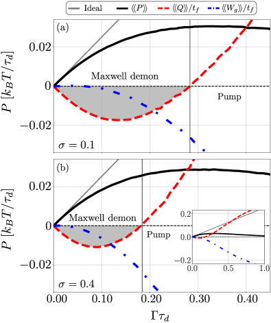
Figure 6: Energy fluxes as functions of $\Gamma\tau_{d}$ where $\Gamma$ is varied and $\tau_{d}$ is fixed. The noise is chosen as $\sigma=0.1$ and $\sigma=0.4$ in (a) and (b), respectively. The system is operated as a Maxwell demon in the gray, shaded regions as the heat is negative there. This is indicated to the left of the thin, black vertical line. To the right of this line, the system is behaving like an electron pump, where the gate voltages ($W_{g}$) are used to transfer electrons against the voltage bias. The ideal case [i.e. Eq. (12)] is represented by the thin, gray line. The inset in (b) shows a zoom-out of the plot. For each point in the plots, $\Gamma t_{f}=100$, and $eV/k_{B}T=2.8$ which roughly corresponds to the maximum in the ideal case, Eq. (13b).

Figure 6 visualizes the same energy fluxes as Fig. 5, but as functions of $\Gamma\tau_{d}$ keeping $\tau_{d}$ fixed. We present two cases with different noise levels. We see how the tunneling rate affects the ability to operate the system in accordance with the ideal cycle. The ideal case is recovered for $\Gamma\tau_{d}\lesssim 0.05$. In this regime, the detector can resolve the electron trajectories. Thereby, we can afford to slightly increase $\Gamma$ and observe an increase of $\langle\!\langle P\rangle\!\rangle$ because of a larger number of transferred electrons per unit time. Increasing $\Gamma$ further, the detector can no longer resolve the trajectories. This trade-off results in a non-monotonic behavior of the power. When $\Gamma\rightarrow\infty$, $\langle\!\langle P\rangle\!\rangle\rightarrow 0$ as can be seen in the inset of Fig. 6(b). From Fig. 6(a), we infer that detector delay times $\tau_{d}\lesssim 1$ $\mu$s would generate measurable currents $I\gtrsim 1$ fA through the double dot system. Delay times of such a magnitude are within reach with radio frequency detection techniques.

The gray, shaded regions indicate again where the second law of thermodynamics is seemingly violated. In these regions, the system acts as Maxwell’s demon. Because noise induces heating, the point where $\langle\!\langle Q\rangle\!\rangle=0$ is pushed towards smaller $\Gamma\tau_{d}$ when $\sigma$ is increased. For larger $\sigma$, there is thus a smaller region where the system is operated as a Maxwell demon. For larger $\Gamma$, power is still produced. However, the energy source is no longer provided by heat but by the voltage gates $W_{g}$. In this regime, the system therefore acts as an electron pump Pothier et al. (1992); Martinis et al. (1994); Keller et al. (1996); Giblin et al. (2010).

V Conclusions & outlook

We presented an implementation of Maxwell’s demon in a double quantum dot system. Under ideal operation conditions, i.e. infinitely fast measurement and feedback, electrons are transported against a voltage bias without performing any net work on the electrons. Thus, information is used to convert heat into electrical work. The distributions of produced work and heat are found to be non-Gaussian.

By means of a Monte Carlo method, we have simulated the system under non-ideal operation conditions, i.e. having delay and noise in the occupation measurements of the dots. Delay slows the operation down, decreasing the produced electrical power, while noise mainly results in heating. The electron trajectories can be fully resolved when having small electron tunneling rates, and the system can be operated in the ideal regime. Slightly increasing the rates, the system is still operated as a Maxwell demon, but it is no longer expected to recover the ideal power production. Further increasing the tunneling rates, the electron trajectories can no longer be resolved, and the operation starts to resemble an electron pump.

Promising avenues to pursue include the quantum regime, where backaction of the measurement has to be taken into account, as well as the quantum-to-classical transition.

Appendix A Monte Carlo simulation

A.1 Rate equation

The system state $S(t)$ is governed by the rate equation $\boldsymbol{\dot{\rho}}(t)=\mathcal{L}\left[D(t)\right]\boldsymbol{\rho}(t)$, where the Liouvillian $\mathcal{L}\left[D(t)\right]$ is dependent on the level setting $D(t)=0,1,2$,

$$\mathcal{L}\left[0\right]=\begin{pmatrix}-\gamma^{(i)}_{L}(\epsilon_{0})\!-\!\gamma^{(i)}_{R}(\epsilon_{u})&\gamma^{(o)}_{L}(\epsilon_{0})&\gamma^{(o)}_{R}(\epsilon_{u})\\ \gamma^{(i)}_{L}(\epsilon_{0})&-\gamma^{(o)}_{L}(\epsilon_{0})&0\\ \gamma^{(i)}_{R}(\epsilon_{u})&0&-\gamma^{(o)}_{R}(\epsilon_{u})\end{pmatrix},$$ (26)

$$\mathcal{L}\left[1\right]=$$ (27)

$$\begin{pmatrix}-\gamma^{(i)}_{L}(\epsilon_{l})\!-\!\gamma^{(i)}_{R}(\epsilon_{l})&\gamma^{(o)}_{L}(\epsilon_{l})&\gamma^{(o)}_{R}(\epsilon_{l})\\ \gamma^{(i)}_{L}(\epsilon_{l})&-\gamma^{(o)}_{L}(\epsilon_{l})\!-\!\gamma&\gamma\\ \gamma^{(i)}_{R}(\epsilon_{l})&\gamma&-\gamma^{(o)}_{R}(\epsilon_{l})\!-\!\gamma\end{pmatrix},$$

and

$$\mathcal{L}\left[2\right]=\begin{pmatrix}-\gamma^{(i)}_{L}(\epsilon_{u})\!-\!\gamma^{(i)}_{R}(\epsilon_{0})&\gamma^{(o)}_{L}(\epsilon_{u})&\gamma^{(o)}_{R}(\epsilon_{0})\\ \gamma^{(i)}_{L}(\epsilon_{u})&-\gamma^{(o)}_{L}(\epsilon_{u})&0\\ \gamma^{(i)}_{R}(\epsilon_{0})&0&-\gamma^{(o)}_{R}(\epsilon_{0})\end{pmatrix},$$ (28)

where the transition rates are given by

$$\gamma^{(i)}_{\alpha}(\epsilon_{j})\!=\!\Gamma_{\alpha}f_{\alpha}\left(\epsilon_{j}\right),\hskip 14.22636pt\gamma^{(o)}_{\alpha}(\epsilon_{j})\!\!=\!\!\Gamma_{\alpha}\left[1\!-\!f_{\alpha}\left(\epsilon_{j}\right)\right].$$ (29)

The superscripts $(i)$ and $(o)$ denote whether a transition is into or out from the double dot, the subscript $\alpha$ specifies whether reservoir $L$ or $R$ is involved, and $j=l,0,u$ defines at which energy the transition occurs.

A.2 Simulation

To simulate the system state at each point in time, we exploit that under a small change of time $\delta t$, where $D(t)$ is constant, it is possible to write

$$\boldsymbol{\rho}(t+\delta t)=\left(\mathbb{1}+\mathcal{L}\left[D(t)\right]\delta t\right)\boldsymbol{\rho}(t).$$ (30)

The change in time $\delta t$ should be small enough such that

$$\gamma_{\alpha}^{(i/o)}(\epsilon_{j})\delta t\ll 1.$$ (31)

Given $S(t)=j$ and $D(t)=k$, with $j,k=0,1,2$, at time $t$, we assign $S(t+\delta t)=i$, $i=0,1,2$, with probability

$$P\left[S(t+\delta t)=i|S(t)\!=\!j,D(t)\!=\!k\right]=\delta_{ij}+\delta t\left(\mathcal{L}[k]\right)_{ij},$$ (32)

which follows from the probability vector $\boldsymbol{\rho}(t+\delta t)$ in Eq. (30). Here, $\delta_{ij}$ is the Kronecker delta, and $\left(\mathcal{L}[k]\right)_{ij}$ is the matrix elements of the Liouvillian given in Eqs. (26)-(28). Before the next time step of the simulation, $d(t+\delta t)$ and $D(t+\delta t)$ must be calculated: First, $m(t+\delta t)$ is computed by Eq. (24). Then a random number is drawn according to Eq. (23) and assigned to $d(t+\delta t)$. Finally, $D(t+\delta t)$ is determined by Eq. (25).

References

- Knott (1911) C. G. Knott, Life and Scientific Work of Peter Guthrie Tait (Cambridge University Press, 1911).
- Maxwell (1871) J. C. Maxwell, Theory of heat (Longmans, Green, and Co., 1871).
- Maruyama et al. (2009) K. Maruyama, F. Nori, and V. Vedral, “Colloquium: The physics of Maxwell’s demon and information,” Rev. Mod. Phys. 81, 1 (2009).
- Bennett (1982) C. H. Bennett, “The thermodynamics of computation-a review,” Int. J. Theor. Phys. 21, 905 (1982).
- Landauer (1961) R. Landauer, “Irreversibility and heat generation in the computing process,” IBM J. Res. Dev. 5, 183 (1961).
- Bustamante et al. (2005) C. Bustamante, J. Liphardt, and F. Ritort, “The nonequilibrium thermodynamics of small systems,” Phys. Today 8, 43 (2005).
- Seifert (2008) U. Seifert, “Stochastic thermodynamics: principles and perspectives,” Eur. Phys. J. B 64, 423 (2008).
- Seifert (2012) U. Seifert, “Stochastic thermodynamics, fluctuation theorems and molecular machines,” Rep. Prog. Phys. 75, 126001 (2012).
- Horowitz and Gingrich (2020) J. M. Horowitz and T. R. Gingrich, “Thermodynamic uncertainty relations constrain non-equilibrium fluctuations,” Nat. Phys. 16, 15 (2020).
- Leff and Rex (2002) H. Leff and A. F. Rex, eds., Maxwell’s Demon 2 Entropy, Classical and Quantum Information, Computing (CRC Press, Boca Raton, 2002).
- Sagawa (2012) T. Sagawa, “Thermodynamics of information processing in small systems,” Prog. Theor. Phys. 127, 1 (2012).
- Parrondo et al. (2015) J. M. R. Parrondo, J. M. Horowitz, and T. Sagawa, “Thermodynamics of information,” Nat. Phys. 11, 131 (2015).
- Potts and Samuelsson (2019a) P. P. Potts and P. Samuelsson, “Thermodynamic uncertainty relations including measurement and feedback,” Phys. Rev. E 100, 052137 (2019a).
- Sagawa and Ueda (2008) T. Sagawa and M. Ueda, “Second law of thermodynamics with discrete quantum feedback control,” Phys. Rev. Lett. 100, 080403 (2008).
- Ponmurugan (2010) M. Ponmurugan, “Generalized detailed fluctuation theorem under nonequilibrium feedback control,” Phys. Rev. E 82, 031129 (2010).
- Sagawa and Ueda (2012a) T. Sagawa and M. Ueda, “Nonequilibrium thermodynamics of feedback control,” Phys. Rev. E 85, 021104 (2012a).
- Sagawa and Ueda (2012b) T. Sagawa and M. Ueda, “Fluctuation theorem with information exchange: Role of correlations in stochastic thermodynamics,” Phys. Rev. Lett. 109, 180602 (2012b).
- Sourabh et al. (2012) L. Sourabh, R. Shubhashis, and A. M. Jayannavar, “Fluctuation theorems in the presence of information gain and feedback,” J. Phys. A 45, 065002 (2012).
- Abreu and Seifert (2012) D. Abreu and U. Seifert, “Thermodynamics of genuine nonequilibrium states under feedback control,” Phys. Rev. Lett. 108, 030601 (2012).
- Potts and Samuelsson (2018) P. P. Potts and P. Samuelsson, “Detailed fluctuation relation for arbitrary measurement and feedback schemes,” Phys. Rev. Lett. 121, 210603 (2018).
- Toyabe et al. (2010) S. Toyabe, T. Sagawa, M. Ueda, E. Muneyuki, and M. Sano, “Experimental demonstration of information-to-energy conversion and validation of the generalized Jarzynski equality,” Nat. Phys. 6, 988 (2010).
- Serreli et al. (2007) V. Serreli, C. F. Lee, E. R. Kay, and D. A. Leigh, “A molecular information ratchet,” Nature 445, 523 (2007).
- Vidrighin et al. (2016) M. D. Vidrighin, O. Dahlsten, M. Barbieri, M. S. Kim, V. Vedral, and I. A. Walmsley, “Photonic Maxwell’s demon,” Phys. Rev. Lett. 116, 050401 (2016).
- Koski et al. (2014a) J. V. Koski, V. F. Maisi, J. P. Pekola, and D. V. Averin, “Experimental realization of a Szilard engine with a single electron,” Proc. Natl. Acad. Sci. U.S.A. 111, 13786 (2014a).
- Koski et al. (2014b) J. V. Koski, V. F. Maisi, T. Sagawa, and J. P. Pekola, “Experimental observation of the role of mutual information in the nonequilibrium dynamics of a Maxwell demon,” Phys. Rev. Lett. 113, 030601 (2014b).
- Chida et al. (2017) K. Chida, S. Desai, K. Nishiguchi, and A. Fujiwara, “Power generator driven by Maxwell’s demon,” Nat. Commun. 8, 15310 (2017).
- Koski et al. (2015) J. V. Koski, A. Kutvonen, I. M. Khaymovich, T. Ala-Nissila, and J. P. Pekola, “On-chip Maxwell’s demon as an information-powered refrigerator,” Phys. Rev. Lett. 115, 260602 (2015).
- Kumar et al. (2018) A. Kumar, T.-Y. Wu, F. Giraldo, and D. S. Weiss, “Sorting ultracold atoms in a three-dimensional optical lattice in a realization of Maxwell’s demon,” Nature 561, 83 (2018).
- Ribezzi-Crivellari and Ritort (2019) M. Ribezzi-Crivellari and F. Ritort, “Large work extraction and the Landauer limit in a continuous Maxwell demon,” Nat. Phys. 15, 660 (2019).
- Cottet et al. (2017) N. Cottet, S. Jezouin, L. Bretheau, P. Campagne-Ibarcq, Q. Ficheux, J. Anders, A. Auffèves, R. Azouit, P. Rouchon, and B. Huard, “Observing a quantum Maxwell demon at work,” Proc. Natl. Acad. Sci. U.S.A. 114, 7561 (2017).
- Masuyama et al. (2018) Y. Masuyama, K. Funo, Y. Murashita, A. Noguchi, S. Kono, Y. Tabuchi, R. Yamazaki, M. Ueda, and Y. Nakamura, “Information-to-work conversion by Maxwell’s demon in a superconducting circuit quantum electrodynamical system,” Nat. Commun. 9, 1291 (2018).
- Naghiloo et al. (2018) M. Naghiloo, J. J. Alonso, A. Romito, E. Lutz, and K. W. Murch, “Information gain and loss for a quantum Maxwell’s demon,” Phys. Rev. Lett. 121, 030604 (2018).
- Gustavsson et al. (2006) S. Gustavsson, R. Leturcq, B. Simovič, R. Schleser, T. Ihn, P. Studerus, K. Ensslin, D. C. Driscoll, and A. C. Gossard, “Counting statistics of single electron transport in a quantum dot,” Phys. Rev. Lett. 96, 076605 (2006).
- Lu et al. (2003) W. Lu, Z. Ji, L. Pfeiffer, K. W. West, and A. J. Rimberg, “Real-time detection of electron tunnelling in a quantum dot,” Nature 423, 422 (2003).
- Fujisawa et al. (2004) T. Fujisawa, T. Hayashi, Y. Hirayama, H. D. Cheong, and Y. H. Jeong, “Electron counting of single-electron tunneling current,” Appl. Phys. Lett. 84, 2343–2345 (2004).
- Schleser et al. (2004) R. Schleser, E. Ruh, T. Ihn, K. Ensslin, D. C. Driscoll, and A. C. Gossard, “Time-resolved detection of individual electrons in a quantum dot,” Appl. Phys. Lett. 85, 2005 (2004).
- Vandersypen et al. (2004) L. M. K. Vandersypen, J. M. Elzerman, R. N. Schouten, L. H. Willems van Beveren, R. Hanson, and L. P. Kouwenhoven, “Real-time detection of single-electron tunneling using a quantum point contact,” Appl. Phys. Lett. 85, 4394 (2004).
- Fujisawa et al. (2006) T. Fujisawa, T. Hayashi, R. Tomita, and Y. Hirayama, “Bidirectional counting of single electrons,” Science 312, 1634 (2006).
- Averin et al. (2011) D. V. Averin, M. Möttönen, and J. P. Pekola, “Maxwell’s demon based on a single-electron pump,” Phys. Rev. B 84, 245448 (2011).
- Schaller et al. (2011) G. Schaller, C. Emary, G. Kiesslich, and T. Brandes, “Probing the power of an electronic Maxwell’s demon: single-electron transistor monitored by a quantum point contact,” Phys. Rev. B 84, 085418 (2011).
- Schaller et al. (2018) G. Schaller, J. Cerrillo, G. Engelhardt, and P. Strasberg, “Electronic Maxwell demon in the coherent strong-coupling regime,” Phys. Rev. B 97, 195104 (2018).
- Strasberg et al. (2013) P. Strasberg, G. Schaller, T. Brandes, and M. Esposito, “Thermodynamics of a physical model implementing a Maxwell demon,” Phys. Rev. Lett. 110, 040601 (2013).
- Kutvonen et al. (2016) A. Kutvonen, J. Koski, and T. Ala-Nissila, “Thermodynamics and efficiency of an autonomous on-chip Maxwell’s demon,” Sci. Rep. 6, 21126 (2016).
- Strasberg et al. (2018) P. Strasberg, G. Schaller, T. L. Schmidt, and M. Esposito, “Fermionic reaction coordinates and their application to an autonomous Maxwell demon in the strong-coupling regime,” Phys. Rev. B 97, 205405 (2018).
- Erdman et al. (2018) P. A. Erdman, B. Bhandari, R. Fazio, J. P. Pekola, and F. Taddei, “Absorption refrigerators based on coulomb-coupled single-electron systems,” Phys. Rev. B 98, 045433 (2018).
- Sánchez et al. (2019) R. Sánchez, P. Samuelsson, and P. P. Potts, “Autonomous conversion of information to work in quantum dots,” Phys. Rev. Research 1, 033066 (2019).
- Levitov et al. (1996) L. S. Levitov, H. Lee, and G. B. Lesovik, “Electron counting statistics and coherent states of electric current,” J. Math. Phys. 37, 4845 (1996).
- Schaller (2014) G. Schaller, Open quantum systems far from equilibrium, Vol. 881 (Springer, 2014).
- Corless et al. (1996) R. M. Corless, G. H. Gonnet, D. E. G. Hare, David J. Jeffrey, and D. E. Knuth, “On the lambert W function,” Adv. Comput. Math. 5, 329 (1996).
- Wagner et al. (2017) T. Wagner, P. Strasberg, J. C. Bayer, E. P. Rugeramigabo, T. Brandes, and R. J. Haug, “Strong suppression of shot noise in a feedback-controlled single-electron transistor,” Nat. Nanotechnol. 12, 218 (2017).
- Maisi et al. (2014) V. F. Maisi, D. Kambly, C. Flindt, and J. P. Pekola, “Full counting statistics of Andreev tunneling,” Phys. Rev. Lett. 112, 036801 (2014).
- Maisi et al. (2016) V. F. Maisi, A. Hofmann, M. Röösli, J. Basset, C. Reichl, W. Wegscheider, T. Ihn, and K. Ensslin, “Spin-orbit coupling at the level of a single electron,” Phys. Rev. Lett. 116, 136803 (2016).
- Fujita et al. (2016) T. Fujita, P. Stano, G. Allison, K. Morimoto, Y. Sato, M. Larsson, J.-H. Park, A. Ludwig, A. D. Wieck, A. Oiwa, and S. Tarucha, “Signatures of hyperfine, spin-orbit, and decoherence effects in a Pauli spin blockade,” Phys. Rev. Lett. 117, 206802 (2016).
- Gingrich et al. (2016) T. R. Gingrich, J. M. Horowitz, N. Perunov, and J. L. England, “Dissipation bounds all steady-state current fluctuations,” Phys. Rev. Lett. 116, 120601 (2016).
- Potts and Samuelsson (2019b) P. P. Potts and P. Samuelsson, “Thermodynamic uncertainty relations including measurement and feedback,” Phys. Rev. E 100, 052137 (2019b).
- Van Vu and Hasegawa (2020) T. Van Vu and Y. Hasegawa, “Uncertainty relation under information measurement and feedback control,” J. Phys. A: Math. Theor. 53, 075001 (2020).
- Küng et al. (2012) B. Küng, C. Rössler, M. Beck, M. Marthaler, D. S. Golubev, Y. Utsumi, T. Ihn, and K. Ensslin, “Irreversibility on the level of single-electron tunneling,” Phys. Rev. X 2, 011001 (2012).
- Pothier et al. (1992) H. Pothier, P. Lafarge, C. Urbina, D. Esteve, and M. H. Devoret, “Single-electron pump based on charging effects,” EPL 17, 249 (1992).
- Koski et al. (2013) J. V. Koski, T. Sagawa, O.-P. Saira, Y. Yoon, A. Kutvonen, P. Solinas, M. Möttönen, T. Ala-Nissila, and J. P. Pekola, “Distribution of entropy production in a single-electron box,” Nat. Phys. 9, 644 (2013).
- Martinis et al. (1994) J. M. Martinis, M. Nahum, and H. D. Jensen, “Metrological accuracy of the electron pump,” Phys. Rev. Lett. 72, 904 (1994).
- Keller et al. (1996) M. W. Keller, J. M. Martinis, N. M. Zimmerman, and A. H. Steinbach, “Accuracy of electron counting using a 7 junction electron pump,” Appl. Phys. Lett. 69, 1804 (1996).
- Giblin et al. (2010) S. P. Giblin, S. J. Wright, J. D. Fletcher, M. Kataoka, M. Pepper, T. J. B. M. Janssen, D. A. Ritchie, C. A. Nicoll, D. Anderson, and G. A. C. Jones, “An accurate high-speed single-electron quantum dot pump,” New J. Phys. 12, 073013 (2010).