The Casimir effect for fermionic currents in conical rings with applications to graphene ribbons

Abstract

We investigate the combined effects of boundaries and topology on the vacuum expectation values (VEVs) of the charge and current densities for a massive 2D fermionic field confined on a conical ring threaded by a magnetic flux. Different types of boundary conditions on the ring edges are considered for fields realizing two inequivalent irreducible representations of the Clifford algebra. The related bound states and zero energy fermionic modes are discussed. The edge contributions to the VEVs of the charge and azimuthal current densities are explicitly extracted and their behavior in various asymptotic limits is considered. On the ring edges the azimuthal current density is equal to the charge density or has an opposite sign. We show that the absolute values of the charge and current densities increase with increasing planar angle deficit. Depending on the boundary conditions, the VEVs are continuous or discontinuous at half-integer values of the ratio of the effective magnetic flux to the flux quantum. The discontinuity is related to the presence of the zero energy mode. By combining the results for the fields realizing the irreducible representations of the Clifford algebra, the charge and current densities are studied in parity and time-reversal symmetric fermionic models. If the boundary conditions and the phases in quasiperiodicity conditions for separate fields are the same the total charge density vanishes. Applications are given to graphitic cones with edges (conical ribbons).

1 Introduction

In the last decade the two-dimensional (2D) fermionic models have attracted considerable attention, both from the experimental and theoretical points of view. Besides being simplified models in particles physics, they also appear as effective theories describing low-energy excitations of the electronic subsystem in a number of condensed matter systems [1]-[4]. The condensed matter realizations of 2D fermions include Weyl semimetals, graphene family materials (graphene, silicene, germanene, stanene), topological insulators, high-temperature superconductors and d-density-wave states. The dynamics of the low-energy charge carriers in these systems is governed by the Dirac equation with the Fermi velocity appearing instead of the velocity of light [5]-[7]. Other examples of the systems with Dirac fermions include ultracold atoms confined by lattice potentials, nano-patterned 2D electron gases and photonic crystals. An important advantage with these artificial systems is that the corresponding symmetry and parameters are relatively easy to control. This provides new opportunities for studying the influence of those parameters on the dynamics of Dirac quasiparticles. The interesting effects induced by the change of the parameters include topological phase transitions, merging of the Dirac points, generation of the anisotropy of the hopping parameters.

The emergence of Dirac fermions in condensed matter systems provides an interesting possibility to observe different kinds of effects in the system of interacting fields. Here we have a situation typical for braneworld models in high-energy physics where a part of the fields are confined on hypersurface (branes) whereas other fields propagate in the bulk. An example is the set of 2D fermionic and 3D electromagnetic field. In quantum field theory, the interaction of the fermionic field, confined on a surface, with the fluctuations of the bulk quantized fields gives rise to the Casimir type shifts in the expectation values of physical observables (for the Casimir effect and its applications in high-energy and condensed matter physics see [8]). In recent years, the Casimir effect in systems involving graphene structures as boundaries have seen novel developments (see [9, 10] and [11] for reviews). In [10] it has been shown that the various electronic phases of graphene family materials, tunable by external fields, lead to different scaling laws and significant magnitude changes for the Casimir forces. These features can be used to probe the 2D Dirac physics of the corresponding materials. The topologically and boundary induced effects in interacting fermionic systems were discussed in [12, 13].

In Refs. [9, 10, 11] the Casimir effect is considered for the electromagnetic field. The role of the 2D fermionic field was reduced to the generation of boundary condition on the quantized electromagnetic field. In graphene family materials with edges (nanoribbons) or with nontrivial spatial topology (nanotubes and nanorings) the Casimir type effects appear for the quantum 2D fermionic field as well. The topological Casimir effect for the fermionic condensate, for the vacuum expectation values (VEVs) of the energy-momentum tensor and of the current density in cylindrical and toroidal nanotubes has been investigated in [14, 15]. The finite temperature effects were discussed in [16]. In finite length nanotubes, in addition to the topological parts, edge-induced Casimir contributions are present. In carbon nanotubes, these contributions depend on the chirality of the tube and have been studied in [17]-[19]. The Casimir effect in a more complicated geometry of hemisphere capped tubes was considered in [20]. The condensed matter realizations of 2D fermions with curved geometries can be used to model the influence of the gravitational field on the quantum matter (for various types of mechanisms of the generation of curvature in graphene and the related effects see [21]). Both the topological and boundary-induced Casimir effects for the charge and current densities of a fermionic field confined on curved graphene tubes with locally anti-de Sitter geometry have been discussed in [22].

In the present paper we investigate the effects of planar angle deficit on the VEVs of the charge and current densities for a 2D fermionic field confined on a conical ring threaded by a magnetic flux. Among the condensed matter realizations of this system are the graphitic cones. These structures are obtained from a graphene sheet by cutting one or more sectors with the angle $\pi/3$ and gluing the two edges of the remaining sector. The corresponding planar angle deficit is given by $\pi n_{c}/3$, with $n_{c}=1,2,\ldots,5$ being the number of the removed sectors. The graphitic cones with all these values of the angle deficit were observed experimentally in both the forms as caps on the ends of the nanotubes and as free-standing structures (see, for instance, [23]). The electronic properties of graphitic cones have been discussed in [24]-[31]. The background geometry under consideration in the present paper with 2D fermionic field corresponds to the continuum description of finite radius graphitic cones with cutted apex. Some limiting cases have been considered previously in the literature. The vacuum polarization effects in the boundary-free geometry with applications to graphitic cones have been discussed in [32]-[35]. The zero temperature fermionic condensate, the expectation values of the charge and current densities and of the energy-momentum tensor for a conical geometry with a single circular boundary where studied in [33]-[35]. The combined effects of the edge and of finite temperature have been considered in [36]. The ground state fermionic charge and current densities in planar rings were investigated in [37].

The organization of the paper is as follows. In the next section the field, background geometry and the mode functions for a fermionic field are presented. In section 3 these modes are used for the evaluation of the VEVs of the charge and current densities in conical rings. Different representations of the VEVs are given and their properties are investigated. Several limiting cases and asymptotics are discussed in section 4. Numerical examples for the behavior of both the charge and current densities are presented. The charge and current densities for the fermionic field realizing the second irreducible representation of the Clifford algebra are considered in section 5. Applications are given to 2D fermionic systems with parity and time-reversal symmetry and to graphene nanocones. The main results are summarized in section 6. The bound states for different boundary conditions on the edges of the ring and their contributions to the VEVs of the charge and current densities are discussed in appendix A. In appendix B we consider the contribution of the special mode for half-integer values of the parameter related to the enclosed magnetic flux and to the phase in the periodicity condition along the azimuthal direction.

2 Problem setup and the fermionic modes

For the background geometry under consideration the (2+1)-dimensional line element is given by

$$ds^{2}=g_{\mu\nu}dx^{\mu}dx^{\nu}=dt^{2}-dr^{2}-r^{2}d\phi^{2}\ ,$$ (2.1)

where the cylindrical spatial coordinates $r$ and $\phi$ vary in the ranges $r\geqslant 0$ and $0\leqslant\phi\leqslant\phi_{0}$. The special case $\phi_{0}=2\pi$ corresponds to the (2+1)-dimensional Minkwoski spacetime described in cylindrical coordinates. For $\phi_{0}<2\pi$, the line element describes a cone with planar angle deficit $2\pi-\phi_{0}$ and with the apex at $r=0$.

As a quantum field we consider a charged fermionic field $\psi(x)$ in the irreducible representation of the Clifford algebra. The latter is realized by two-component spinors. Additionally, the presence of an external classical abelian gauge field $A_{\mu}$ will be assumed. The dynamics of the field is governed by the Dirac equation

$$\left(i\gamma^{\mu}D_{\mu}-sm\right)\psi(x)=0.$$ (2.2)

The gauge extended covariant derivative is defined as $D_{\mu}=\partial_{\mu}+\Gamma_{\mu}+ieA_{\mu}$, with $\Gamma_{\mu}$ being the spin connection and $e$ being the charge of the field quanta. In (2.2) we have introduced the parameter $s$, with the values $s=+1$ and $s=-1$, corresponding to two inequivalent irreducible representations of the Clifford algebra in $(2+1)$-dimensions (see also section 5). In the coordinate system under consideration for the Dirac matrices in (2.2) we use the representation

$$\gamma^{0}=\left(\begin{array}[]{cc}1&0\\ 0&-1\end{array}\right),\quad\gamma^{l}=\frac{i^{2-l}}{r^{l-1}}\left(\begin{array}[]{cc}0&e^{-iq\phi}\\ (-1)^{l-1}e^{iq\phi}&0\end{array}\right),$$ (2.3)

where $l=1,2$ and $q=2\pi/\phi_{0}$.

It will be assumed that the field is confined in the region $a\leq r\leq b$ (conical ring, the geometry of the problem is depicted in figure 1). On the edges of the ring the boundary conditions

$$\left(1+i\lambda_{r}n_{\mu}\gamma^{\mu}\right)\psi(x)=0,\;r=a,b,$$ (2.4)

will be imposed. Here $n_{\mu}$ is the inward pointing unit vector normal to the boundary and the parameters $\lambda_{a}$ and $\lambda_{b}$ take the values $\pm 1$. For the boundary at $r=u$, $u=a,b$, and in the region under consideration the normal is given by $n_{\mu}=n_{u}\delta_{\mu}^{1}$, where

$$n_{a}=-1,\;n_{b}=1.$$ (2.5)

It can be shown that, as a consequence of the conditions (2.4), on the boundaries we get $n_{\mu}j^{\mu}=0$ with $j^{\mu}=e\bar{\psi}\gamma^{\mu}\psi$ being the current density and $\bar{\psi}=\psi^{\dagger}\gamma^{0}$ is the Dirac adjoint. This means that the normal component of the fermionic current vanishes on the edges and, consequently, the dynamics is completely determined by the field equation and the boundary conditions. The special case with $\lambda_{r}=1$, $r=a,b$, corresponds to the MIT bag boundary condition (or infinite mass boundary condition in the condensed matter context) on both the edges. Comparing the analytical results on the electronic properties of circular graphene quantum dots derived within the Dirac model with the bag boundary condition to those obtained from the tight-binding model, the authors of [38] have found a good qualitative agreement between those two approaches. Considering different boundary conditions in the continuous model for graphene devices and comparing with the experiments, a similar conclusion is made in [39]. Another special case with $\lambda_{r}=-1$ was considered in [40]. More general boundary conditions for the confinement of fermions and their realizations in graphene made structures have been discussed in [41].

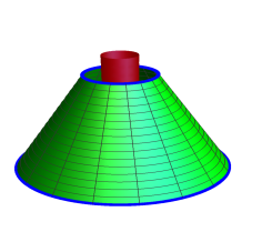
Figure 1: Conical ring with the edges $r=a$ and $r=b$ threaded by a magnetic flux.

The background geometry has nontrivial topology and, in addition to the boundary conditions on the ring edges, one needs to specify the periodicity condition along the azimuthal direction. We will assume the condition

$$\psi(t,r,\phi+\phi_{0})=e^{2\pi i\chi}\psi(t,r,\phi),$$ (2.6)

with a general phase $2\pi\chi$. The special cases $\chi=0$ and $\chi=1/2$ correspond to untwisted and twisted fermionic fields. The values for the parameter $\chi$ realized in graphene cones will be discussed in section 5. As it will be seen below, the nontrivial phase in (2.6) can be interpreted in terms of the fictitious flux threading the ring.

Here we are interested in the VEVs of the charge and current densities induced by a magnetic flux threading the conical ring. The magnetic field is localized inside the region $r<a$ and its influence on the characteristics of the fermionic vacuum is purely topological. This is an Aharonov-Bohm type effect related to the nontrivial topology of the background space. In the region under consideration, $a\leq r\leq b$, the covariant components of the vector potential of the gauge field in the system of coordinates $(t,r,\phi)$ are given by $A_{\mu}=(0,0,A)$. Note that for the corresponding physical component one has $A_{\phi}=-A/r$. The magnetic flux enclosed by the ring is expressed in terms of the covariant component as $\Phi=-\phi_{0}A$. The physical effects on the ring are completely determined by this flux and they do not depend on the radial distribution of the flux in the region $r<a$.

The VEV of the current density, $\langle 0|j^{\mu}(x)|0\rangle\equiv\langle j^{\mu}(x)\rangle$, can be evaluated by using the relation

$$\langle j^{\mu}(x)\rangle=-\frac{e}{2}\mathrm{Tr}(\gamma^{\mu}S^{(1)}(x,x)),$$ (2.7)

where the trace in the right-hand side is over spinor indices and $S^{(1)}(x,x^{\prime})$ is the fermion two-point function. Its spinorial components, with spinor indices $i$ and $k$, are defined as the VEV $S_{ik}^{(1)}(x,x^{\prime})=\langle 0|[\psi_{i}(x),\bar{\psi}_{k}(x^{\prime})]|0\rangle$. Let $\{\psi_{\sigma}^{(+)}(x),\psi_{\sigma}^{(-)}(x)\}$ be the complete set of the positive and negative energy fermionic mode functions, obeying the field equation (2.2), the boundary conditions (2.4) and the periodicity condition (2.6). They are specified by the set of quantum numbers $\sigma$. Expanding the field operator in terms of the modes and using the commutation relations for the fermionic annihilation and creation operators, the VEV of the current density is presented in the form of the mode sum

$$\langle j^{\mu}(x)\rangle=-\frac{e}{2}\sum_{\sigma}\sum_{\kappa=-,+}\kappa\bar{\psi}_{\sigma}^{(\kappa)}(x)\gamma^{\mu}\psi_{\sigma}^{(\kappa)}(x),$$ (2.8)

where the terms with $\kappa=+$ and $\kappa=-$ correspond to the contributions of the positive and negative energy modes.

The structure of the mode functions $\psi_{\sigma}^{(\kappa)}(x)$ is similar to that discussed in [36]. They are specified by the quantum numbers $(\gamma,j)$, where $j=\pm 1/2,\pm 3/2,\ldots$ is the total angular momentum and the radial quantum number $\gamma$ determines the energy of the corresponding mode $\kappa E$, with $E=\sqrt{\gamma^{2}+m^{2}}$. Introducing the notation

$$\alpha=\chi+eA/q=\chi-e\Phi/(2\pi),$$ (2.9)

the mode functions are presented in the form

$$\psi_{\sigma}^{(\kappa)}(x)=C_{\kappa}e^{iq(j+\chi)\phi-\kappa iEt}\left(\begin{array}[]{c}g_{\beta_{j},\beta_{j}}(\gamma a,\gamma r)e^{-iq\phi/2}\\ \epsilon_{j}\frac{\gamma e^{iq\phi/2}}{\kappa E+sm}g_{\beta_{j},\beta_{j}+\epsilon_{j}}(\gamma a,\gamma r)\end{array}\right)\ ,$$ (2.10)

where $\epsilon_{j}=1$ for $j>-\alpha$ and $\epsilon_{j}=-1$ for $j<-\alpha$,

$$\beta_{j}=q|j+\alpha|-\epsilon_{j}/2.$$ (2.11)

Note that the part $e\Phi/(2\pi)$ in (2.9) is the ratio of the magnetic flux threading the ring to the flux quantum $\Phi_{0}=2\pi/e$. The functions $g_{\beta_{j},\nu}(\gamma a,\gamma r)$ of the radial coordinate $r$, with the orders $\nu=\beta_{j}$ and $\nu=\beta_{j}+\epsilon_{j}$, is expressed in terms of the Bessel and Neumann functions as:

$$g_{\beta_{j},\nu}(\gamma a,\gamma r)=Y_{\beta_{j}}^{(a)}(\gamma a)J_{\nu}(\gamma r)-J_{\beta_{j}}^{(a)}(\gamma a)Y_{\nu}(\gamma r)\ .$$ (2.12)

For the Bessel and Neumann functions we use the notation

$$f_{\beta_{j}}^{(u)}\left(x\right) = xf_{\beta_{j}}^{\prime}\left(x\right)+[\lambda_{u}n_{u}(\kappa\sqrt{x^{2}+m_{u}^{2}}+sm_{u})-\epsilon_{j}\beta_{j}]f_{\beta_{j}}\left(x\right)$$ (2.13)

$$= \lambda_{u}n_{u}(\kappa\sqrt{x^{2}+m_{u}^{2}}+sm_{u})f_{\beta_{j}}\left(x\right)-\epsilon_{j}xf_{\beta_{j}+\epsilon_{j}}\left(x\right),$$

with $u=a,b$, $f=J,Y$, and $m_{u}=mu$. When the parameter $\alpha$ is equal to an half-integer, the modes with $j\neq-\alpha$ are still given by (2.10). In this case there is a special mode with $j=-\alpha$ which is separately discussed in appendix B.

The coefficients of the linear combination of the cylinder functions in (2.12) are obtained from the boundary condition (2.4) at $r=a$. The further imposition of the boundary condition at $r=b$ determines the eigenvalues of the quantum number $\gamma$ as roots of the equation

$$C_{\beta_{j}}(b/a,\gamma a)\equiv J_{\beta_{j}}^{(a)}\left(\gamma a\right)Y_{\beta_{j}}^{(b)}\left(\gamma b\right)-J_{\beta_{j}}^{(b)}\left(\gamma b\right)Y_{\beta_{j}}^{(a)}\left(\gamma a\right)=0.$$ (2.14)

We will denote by $z_{l}$, $l=1,2,\ldots$, the positive solutions of this equation with respect to $\gamma a$, assuming that $z_{l}<z_{l+1}$. The eigenvalues of $\gamma$ are expressed as $\gamma=\gamma_{l}=z_{l}/a$. Hence, the mode functions are specified by the set of discrete quantum numbers $\sigma=(l,j)$. The energies of the positive and negative energy modes are given as $E_{\kappa}=\kappa E$ with $E=\sqrt{\gamma_{l}^{2}+m^{2}}$. For a given quantum number $j$, the equations (2.14) for the eigenvalues $\gamma_{l}$ of the positive and negative energy modes differ by the change of the energy sign. As it will be discussed in appendix A, depending on the set of the parameters $(s,\lambda_{a},\lambda_{b})$, purely imaginary solutions of the equation (2.14) may present. For all these solutions $\gamma^{2}+m^{2}\geq 0$ and the vacuum state is stable. For a massless field the confinement of the field, in general, induces an energy gap that depends on the geometrical characteristics of the ring. The controllable energy gap plays an important role in graphene ribbons. For large values of $\gamma a\gg 1$ we can use in (2.14) the asymptotic expressions of cylinder functions for large arguments. In the case $\lambda_{a}=-\lambda_{b}$, to the leading order, the equation of the modes is reduced to $\sin\left[\left(b-a\right)\gamma\right]=0$ with $\gamma_{l}\approx\pi l/(b-a)$ for large $l$. For $\lambda_{a}=\lambda_{b}$ and $\gamma a\gg 1$ from (2.14) we get $s(m/\gamma)\sin x+\cos x=0$ with $x=\left(b-a\right)\gamma$. For $\gamma\gg m$ this gives $\gamma_{l}\approx\pi(l+1/2)/(b-a)$.

Let us present the parameter $\alpha$ from (2.9) in the form

$$\alpha=\alpha_{0}+n_{0},\quad|\alpha_{0}|\leq 1/2,$$ (2.15)

where $n_{0}$ is an integer. Redefining $j\rightarrow j+n_{0}$, we see that the solutions $z_{l}$ are functions of $b/a,\alpha_{0},j,s,\lambda_{u},\kappa$: $z_{l}=z_{l}(b/a,s,\lambda_{u},j,\alpha_{0},\kappa)$. By taking into account (2.13) it can be seen that the function $f_{\beta_{j}}^{(u)}\left(x\right)$ for the set $(j,\alpha_{0},\kappa)$ coincides with the function $f_{\beta_{j}}^{(u)}\left(x\right)$ for the set $(-j,-\alpha_{0},-\kappa)$ up to the coefficient $\lambda_{u}n_{u}(\kappa\sqrt{x^{2}+m_{u}^{2}}+sm_{u})/x$. From here it follows that $z_{l}(b/a,s,\lambda_{u},j,\alpha_{0},\kappa)=z_{l}(b/a,s,\lambda_{u},-j,-\alpha_{0},-\kappa)$. In particular, this means that the negative energy solutions for the set $(j,\alpha_{0})$ coincide with the positive energy solutions for $(-j,-\alpha_{0})$. Another relation between the roots for different sets of parameters directly follows from the definition (2.13): $z_{l}(b/a,s,\lambda_{u},j,\alpha_{0},\kappa)=z_{l}(b/a,-s,-\lambda_{u},j,\alpha_{0},-\kappa)$. Combining this with the previous relation we get $z_{l}(b/a,s,\lambda_{u},j,\alpha_{0},\kappa)=z_{l}(b/a,-s,-\lambda_{u},-j,-\alpha_{0},\kappa)$.

To complete the specification of the fermionic modes it remains to determine the normalization coefficient $C_{\kappa}$ in (2.10). It is obtained from the standard orthonormalization condition

$$\int_{a}^{b}dr\int_{0}^{\phi_{0}}d\phi\,r\psi_{\sigma}^{(\kappa)\dagger}(x)\psi_{\sigma^{\prime}}^{(\kappa)}(x)=\delta_{jj^{\prime}}\ \delta_{ll^{\prime}},$$ (2.16)

for fermionic fields. The radial integral involving the square of the cylinder functions $g_{\beta_{j},\nu}(\gamma a,\gamma r)$ is evaluated by using the result from [42]. This leads to the following expression

$$\left|C_{\kappa}\right|^{2}=\frac{\pi qz_{l}}{16a^{2}}\frac{E+\kappa sm}{E}T_{\beta_{j}}^{ab}(z_{l}),$$ (2.17)

where we have defined the function

$$T_{\beta_{j}}^{ab}(z)=\frac{z}{E+\kappa sm}\left[\frac{B_{b}J_{\beta_{j}}^{(a)2}\left(z\right)}{J_{\beta_{j}}^{(b)2}\left(zb/a\right)}-B_{a}\right]^{-1},$$ (2.18)

with

$$B_{u}=u^{2}\left[E-\frac{\kappa\lambda_{u}n_{u}}{u}\left(\frac{E-\kappa sm}{2E}+\epsilon_{j}\beta_{j}\right)\right].$$ (2.19)

In deriving (2.17) we have used the relations

$$g_{\beta_{j},\beta_{j}}(\gamma a,\gamma u) = \frac{2}{\pi}\frac{J_{\beta_{j}}^{(a)}(\gamma a)}{J_{\beta_{j}}^{(u)}(\gamma u)},$$

$$g_{\beta_{j},\beta_{j}+\epsilon_{j}}(\gamma a,\gamma u) = \frac{2\epsilon_{j}}{\pi\gamma}\lambda_{u}n_{u}(\kappa E+sm)\frac{J_{\beta_{j}}^{(a)}(\gamma a)}{J_{\beta_{j}}^{(u)}(\gamma u)},$$ (2.20)

with $u=a,b$.

The model under consideration is specified by the set of parameters $(\chi,A)$. The first one determines the phase in the periodicity condition in the azimuthal direction and the second one determines the magnetic flux enclosed by the ring. These parameters are not separately gauge invariant. Under the gauge transformation $A_{\mu}=A_{\mu}^{\prime}+\partial_{\mu}\omega$, $\psi(x)=\psi^{\prime}(x)e^{-ie\omega}$, with the function $\omega=b_{\mu}x^{\mu}$, a new set is given by $(\chi^{\prime},A^{\prime})=(\chi+eb_{2}/q,A-b_{2})$. However, the parameter $\alpha$, defined by (2.9), is gauge invariant. In particular, in the gauge with $b_{2}=-q\chi/e$ the fermionic field is periodic in the azimuthal direction and the phase $\chi$ is interpreted in terms of a fictitious magnetic flux $-2\pi\chi/e=-\chi\Phi_{0}$. In this sense, the parameter $\alpha$ can be considered as the ratio of the effective magnetic flux to the flux quantum.

3 VEVs of the charge and current densities

3.1 Mode sum

In this section we evaluate the VEVs of the charge and current densities on conical rings. First we assume that all the solutions of the eigenvalue equation (2.14) are real. The modifications in the evaluation procedure required by the presence of imaginary roots are described in appendix A. Having specified the complete set of mode functions (2.10), for the VEV (2.8) one finds the representation

$$\langle j^{\mu}\rangle=-\frac{\pi eq}{32a^{2}}\sum_{j}\sum_{\kappa=\pm}\,\kappa\sum_{l=1}^{\infty}T_{\beta_{j}}^{ab}(z_{l})w_{\mu,\beta_{j}}(z_{l}),$$ (3.1)

where in the summation over $j$ one has $j=\pm 1/2,\pm 3/2,\ldots$. Here for the charge and azimuthal current densities we have defined the functions

$$w_{0,\beta_{j}}(z) = \frac{z}{E}\left[\left(E+\kappa sm\right)g_{\beta_{j},\beta_{j}}^{2}(z,zr/a)+\left(E-\kappa sm\right)g_{\beta_{j},\beta_{j}+\epsilon_{j}}^{2}(z,zr/a)\right],$$

$$w_{2,\beta_{j}}(z) = 2\frac{\kappa\epsilon_{j}z^{2}}{arE}g_{\beta_{j},\beta_{j}}(z,zr/a)g_{\beta_{j},\beta_{j}+\epsilon_{j}}(z,zr/a),$$ (3.2)

with $E=\sqrt{z^{2}/a^{2}+m^{2}}$ and $w_{1,\beta_{j}}(z)=0$. The VEV of the radial current density vanishes. Note that the physical component of the azimuthal current density is given by $\langle j_{\phi}\rangle=r\langle j^{2}\rangle$.

We can see that under the replacements $\beta_{j}\rightleftarrows\beta_{j}+\epsilon_{j}$,$\;\kappa\rightarrow-\kappa$ the function (2.13) transforms as

$$f_{\beta_{j}}^{(u)}\left(u\gamma\right)\rightarrow-\epsilon_{j}\left(\lambda_{u}n_{u}/u\right)(\kappa E+sm)f_{\beta_{j}}^{(u)}\left(u\gamma\right).$$ (3.3)

From here it follows that the roots $z_{l}$ of (2.14) are not changed under those replacements. The same is the case for the product $T_{\beta_{j}}^{ab}(z_{l})w_{\mu,\beta_{j}}(z_{l})$ in (3.1). But the replacements $\beta_{j}\rightleftarrows\beta_{j}+\epsilon_{j}$ are equivalent to the change $(j,\alpha)\rightarrow(-j,-\alpha)$. Hence, we conclude that the VEVs (3.1) are odd periodic functions of the parameter $\alpha$ with the period 1. This implies periodicity with respect to the enclosed magnetic flux with the period of the flux quantum. Of course, this is the well known feature for Aharonov-Bohm type effects.

For half-integer values of the parameter $\alpha$ the contribution of the modes $j\neq-\alpha$ to the VEV $\langle j^{\mu}\rangle$ is still given by expression (3.1) and the contribution coming from the special mode $j=-\alpha$ is investigated in appendix B. Redefining the summation variable $j$ in (3.1), it is sufficient to consider the values $\alpha=\pm 1/2$. For definiteness consider the case $\alpha=1/2$. Let us present the series over $j$ in (3.8) as $\sum_{j}\kappa f(\beta_{j},\beta_{j}+\epsilon_{j},\kappa)$ with $j\neq-1/2$. In the part over the negative values $j$ we pass to a new summation variable, $j\rightarrow-j-1$. This transforms the series to the form $\sum_{j>0}\kappa\left[f(\beta_{j},\beta_{j}+\epsilon_{j},\kappa)+f(\beta_{j}+\epsilon_{j},\beta_{j},\kappa)\right]$. But as it has been explained above $f(\beta_{j}+\epsilon_{j},\beta_{j},\kappa)=f(\beta_{j},\beta_{j}+\epsilon_{j},-\kappa)$ and the expression under the summation sign is an odd function of $\kappa$. Hence, the contributions from the positive and negative energy modes cancel each other and the modes with $j\neq-\alpha$ do not contribute to the charge and current densities for half-integer values of $\alpha$. As it is shown in appendix B the same is the case for the contribution of the mode $j=-\alpha$ if $\lambda_{a}=\lambda_{b}$. For $\lambda_{a}=-\lambda_{b}$ and $j=-\alpha$ the positive eigenvalues of $\gamma$ are zeros of the function $\sin[\gamma(b-a)]$ and, again, their contribution vanishes. In the case $\lambda_{a}=-\lambda_{b}$ the only nonzero contribution comes from the zero energy mode and the corresponding charge density is given by (B.8). Hence, for half-integer values of the parameter $\alpha$ the charge and current densities vanish for the boundary conditions with $\lambda_{a}=\lambda_{b}$ and are determined by $\langle j^{0}\rangle=-\lambda_{a}\langle j_{\phi}\rangle=\langle j^{0}\rangle_{\mathrm{(s)}}^{(0)}$, with $\langle j^{0}\rangle_{\mathrm{(s)}}^{(0)}$ from (B.8), for $\lambda_{a}=-\lambda_{b}$.

Returning to the general case for $\alpha$ and by using the relations (2.20), for the charge density on the ring edges one finds

$$\langle j^{0}\rangle_{r=u}=-\frac{eq}{4\pi a}\sum_{j}\sum_{\kappa=\pm}\,\kappa\sum_{l=1}^{\infty}\gamma_{l}T_{\beta_{j}}^{ab}(z_{l})\frac{E+\kappa sm}{E}\frac{J_{\beta_{j}}^{(a)2}(\gamma a)}{J_{\beta_{j}}^{(u)2}(\gamma u)}.$$ (3.4)

The azimuthal current density on the edge is related to the corresponding charge density by the simple formula

$$\langle j_{\phi}\rangle_{r=u}=\lambda_{u}n_{u}\langle j^{0}\rangle_{r=u}.$$ (3.5)

For planar rings this relation in the case $\lambda_{u}=1$ has been already mentioned in [37].

3.2 Integral representation

The representation (3.1) has two disadvantages: the roots $z_{l}$ are given implicitly, as zeros of the function (2.14), and the terms with large $l$ are highly oscillatory. Both of these difficulties can be overcome by making use of the summation formula [43] (see also [44])

$$\sum_{l=1}^{\infty}w(z_{l})T_{\beta_{j}}^{ab}(z_{l}) = \frac{4}{\pi^{2}}\int_{0}^{\infty}{dz\,}\frac{w(z)}{J_{\beta_{j}}^{(a)2}\left(z\right)+Y_{\beta_{j}}^{(a)2}\left(z\right)}-\frac{2}{\pi}\underset{z=0}{\mathrm{Res}}\left[\frac{w(z)H_{\beta_{j}}^{(1b)}\left(zb/a\right)}{C_{\beta_{j}}(b/a,z)H_{\beta_{j}}^{(1a)}\left(z\right)}\right]$$ (3.6)

$$-\frac{1}{\pi}\int_{0}^{\infty}dz\,\sum_{p=+,-}\frac{w(ze^{pi\pi/2})K_{\beta_{j}}^{(bp)}(\eta z)/K_{\beta_{j}}^{(ap)}(z)}{K_{\beta_{j}}^{(ap)}\left(z\right)I_{\beta_{j}}^{(bp)}\left(\eta z\right)-I_{\beta_{j}}^{(ap)}(z)K_{\beta_{j}}^{(bp)}(\eta z)}.$$

Here we use the notation (2.13) for the Hankel functions $H_{\nu}^{(1,2)}(x)$ and the notation

$$f_{\beta_{j}}^{(up)}(x)=xf_{\beta_{j}}^{\prime}\left(x\right)+\left\{\lambda_{u}n_{u}\left[\kappa\sqrt{\left(xe^{p\pi i/2}\right)^{2}+m_{u}^{2}}+sm_{u}\right]-\epsilon_{j}\beta_{j}\right\}f_{\beta_{j}}\left(x\right),$$ (3.7)

for the modified Bessel functions $I_{\nu}(x)$ and $K_{\nu}(x)$. The conditions on the function $w(z)$, analytic in the right-half plane $\mathrm{Re}\,z>0$, are formulated in [43]. On the imaginary axis the function $w(z)$ may have branch points. The square root $\sqrt{\left(ze^{p\pi i/2}\right)^{2}+m_{u}^{2}}$ in (3.7) is understood as $\sqrt{m_{u}^{2}-z^{2}}$, for $z<m_{u}$, and as $pi\sqrt{z^{2}-m_{u}^{2}}$ for $z>m_{u}$. From here it follows that $f_{\beta_{j}}^{(u+)}(z)=f_{\beta_{j}}^{(u-)}(z)$ for $z<m_{u}$.

For the series in (3.1) one has $w(z)=w_{\mu,\beta_{j}}(z)$. The functions $w_{\mu,\beta_{j}}(z)$ have branch points $z=\pm im_{a}$ on the imaginary axis and obey the relation $w_{\mu,\beta_{j}}(ze^{-\pi i/2})=-w_{\mu,\beta_{j}}(ze^{\pi i/2})$ for $z<m_{a}$. By using these properties we can see that the positive and negative energy modes give the same contributions to the VEVs of the charge and current densities and they are presented as

$$\langle j^{\mu}\rangle=\langle j^{\mu}\rangle_{a}+\frac{eq}{2\pi^{2}}\sum_{j}\,\int_{m}^{\infty}dx\,\frac{x}{\sqrt{x^{2}-m^{2}}}\mathrm{Re}\left[\frac{V_{\mu,\beta_{j}}^{(a)}(ax,rx)K_{\beta_{j}}^{(b)}(bx)/K_{\beta_{j}}^{(a)}(ax)}{K_{\beta_{j}}^{(a)}\left(ax\right)I_{\beta_{j}}^{(b)}\left(bx\right)-I_{\beta_{j}}^{(a)}(ax)K_{\beta_{j}}^{(b)}(bx)}\right],$$ (3.8)

where

$$V_{0,\beta_{j}}^{(u)}(ux,rx) = \left(sm+i\sqrt{x^{2}-m^{2}}\right)G_{\beta_{j},\beta_{j}}^{(u)2}(ux,rx)+\left(sm-i\sqrt{x^{2}-m^{2}}\right)G_{\beta_{j},\beta_{j}+\epsilon_{j}}^{(u)2}(ux,rx),$$

$$V_{2,\beta_{j}}^{(u)}(ux,rx) = -\frac{2x}{r}G_{\beta_{j},\beta_{j}}^{(u)}(ux,rx)G_{\beta_{j},\beta_{j}+\epsilon_{j}}^{(u)}(ux,rx),$$ (3.9)

with $u=a,b$. The functions in the right-hand sides of (3.9) are defined by

$$G_{\beta_{j},\mu}^{(u)}(x,y)=K_{\beta_{j}}^{(u)}\left(x\right)I_{\mu}\left(y\right)-(-1)^{\mu-\beta_{j}}I_{\beta_{j}}^{(u)}\left(x\right)K_{\mu}\left(y\right),$$ (3.10)

and for the modified Bessel functions $f_{\nu}\left(z\right)=I_{\nu}\left(z\right),K_{\nu}\left(z\right)$ we use the notation

$$f_{\beta_{j}}^{(u)}(z) = zf_{\beta_{j}}^{\prime}\left(z\right)+\left[\lambda_{u}n_{u}\left(i\sqrt{z^{2}-m_{u}^{2}}+sm_{u}\right)-\epsilon_{j}\beta_{j}\right]f_{\beta_{j}}\left(z\right)$$ (3.11)

$$= \delta_{f}zf_{\beta_{j}+\epsilon_{j}}\left(z\right)+\lambda_{u}n_{u}(i\sqrt{z^{2}-m_{u}^{2}}+sm_{u})f_{\beta_{j}}\left(z\right),$$

where $\delta_{I}=1$, $\delta_{K}=-1$, and $u=a,b$. The expressions for the VEVs of the charge and current densities contain a summation over $j$ that enters in the formulas through $\beta_{j}$ defined as (2.11). Redefining the summation variable $j\rightarrow j+n_{0}$, with $n_{0}$ defined by (2.15), we see that the VEVs do not depend on $n_{0}$ and only the fractional part of $\alpha$ is physically relevant. Recall that in deriving (3.8) we have assumed that all the roots of the equation (2.14) are real. In appendix A it is shown that the representation (3.8) is valid also in the presence of imaginary roots corresponding to the bound states.

In (3.8), the part $\langle j^{\mu}\rangle_{a}$ comes from the first term in the right-hand side of (3.6) and is given by the expression

$$\langle j^{\mu}\rangle_{a}=-\frac{eq}{8\pi a^{2}}\sum_{j}\sum_{\kappa=\pm 1}\,\int_{0}^{\infty}{dz\,}\frac{\kappa w_{\mu,\beta_{j}}(z)}{J_{\beta_{j}}^{(a)2}\left(z\right)+Y_{\beta_{j}}^{(a)2}\left(z\right)}.$$ (3.12)

For its physical interpretation we note that the last term in (3.8) tends to zero in the limit $b\rightarrow\infty$. This shows that (3.12) corresponds to the VEV in the region $r\geq a$ for a cone with a single edge $r=a$. By using the identity

$$\frac{g_{\beta_{j},\nu}(z,y)g_{\beta_{j},\rho}(z,y)}{J_{\beta_{j}}^{(a)2}(x)+Y_{\beta_{j}}^{(a)2}(x)}=J_{\nu}(y)J_{\rho}(y)-\frac{1}{2}\sum_{l=1,2}\frac{J_{\beta_{j}}^{(a)}(z)}{H_{\beta_{j}}^{(al)}(z)}H_{\nu}^{(l)}(y)H_{\rho}^{(l)}(y).$$ (3.13)

with $\nu,\rho=\beta_{j},\beta_{j}+\epsilon_{j}$, it can be further decomposed as

$$\langle j^{\mu}\rangle_{a}=\langle j^{\mu}\rangle_{0}+\langle j^{\mu}\rangle_{a}^{\mathrm{(b)}},$$ (3.14)

where the separate parts come from the first and second terms in the right-hand side of (3.13). For the first part one has

$$\langle j^{\mu}\rangle_{0}=-\frac{eq}{4\pi}\sum_{j}\,\int_{0}^{\infty}dx\,\frac{xw_{\mu,\beta_{j}}^{(0)}(rx)}{\sqrt{x^{2}+m^{2}}},$$ (3.15)

with the functions

$$w_{0,\beta_{j}}^{(0)}(z) = sm\left[J_{\beta_{j}}^{2}(z)-J_{\beta_{j}+\epsilon_{j}}^{2}(z)\right],$$

$$w_{2,\beta_{j}}^{(0)}(z) = \frac{2\epsilon_{j}z}{r^{2}}J_{\beta_{j}}(z)J_{\beta_{j}+\epsilon_{j}}(z),$$ (3.16)

and $w_{1,\beta_{j}}^{(0)}(z)=0$. In the part $\langle j^{\mu}\rangle_{a}^{\mathrm{(b)}}$ we rotate the contour of the integration over $z$ by the angles $\pi/2$ and $-\pi/2$ for the terms with $l=1$ and $l=2$, respectively. Introducing the modified Bessel functions we get

$$\langle j^{\mu}\rangle_{a}^{\mathrm{(b)}}=\frac{eq}{2\pi^{2}}\sum_{j}\int_{m}^{\infty}dx\,\frac{x}{\sqrt{x^{2}-m^{2}}}\mathrm{Re}\left[\frac{I_{\beta_{j}}^{(a)}(ax)}{K_{\beta_{j}}^{(a)}(ax)}W_{\mu,\beta_{j}}(rx)\right],$$ (3.17)

with the notations (3.11) and

$$W_{0,\beta_{j}}(rx) = \left(sm+i\sqrt{x^{2}-m^{2}}\right)K_{\beta_{j}}^{2}(rx)+\left(sm-i\sqrt{x^{2}-m^{2}}\right)K_{\beta_{j}+\epsilon_{j}}^{2}(rx),$$

$$W_{2,\beta_{j}}(rx) = \frac{2x}{r}K_{\beta_{j}}(rx)K_{\beta_{j}+\epsilon_{j}}(rx).$$ (3.18)

For the representation $s=1$ and for the boundary condition with $\lambda_{a}=1$, this expression for a single boundary-induced part coincides with the one given in [34] (comparing the formulas here with the results of [34], the replacements $\alpha\rightarrow-\alpha$ and $\alpha_{0}\rightarrow-\alpha_{0}$ should be made; this difference is related to that in [34], for the evaluation of the VEVs for the geometry with a single boundary, the analog of the negative-energy mode functions (2.10) was used with $\alpha$ replaced by $-\alpha$). The part $\langle j^{\mu}\rangle_{0}$ in (3.14) with $0<r<\infty$ corresponds to the VEV in a conical space without boundaries and the contribution $\langle j^{\mu}\rangle_{a}^{\mathrm{(b)}}$ is induced in the region $r\geq a$ by the presence of the edge $r=a$.

Another representation of the VEV (3.15) in the boundary-free conical geometry for the case $s=1$ is provided in [34]. The parameter $s$ enters in (3.15) as a coefficient in the charge density and the corresponding generalization is straightforward with the expression

$$\langle j^{\mu}\rangle_{0}=-\frac{e}{2\pi r}\Big{\{}\sideset{}{{}^{\prime}}{\sum}_{l=1}^{[q/2]}(-1)^{l}\sin(2\pi l\alpha_{0})f_{\mu}\left(2mr\sin(\pi l/q)\right)$$

$$\qquad-\frac{q}{\pi}\int_{0}^{\infty}dy\frac{f_{\mu}\left(2mr\cosh y\right)}{\cosh(2qy)-\cos(q\pi)}\sum_{p=\pm 1}p\cos\left[q\pi\left(1/2-p\alpha_{0}\right)\right]\cosh\left[q\left(1+2p\alpha_{0}\right)y\right]\Big{\}},$$ (3.19)

where $[q/2]$ means the integer part of $q/2$, the prime on the summation sign means that for even $q$ the term with $l=q/2$ should be taken with an additional coefficient 1/2, and we have introduced the functions

$$f_{0}(z) = sme^{-z},$$

$$f_{2}(z) = 2m^{2}(1+z)e^{-z}/z^{2}.$$ (3.20)

The boundary-free contributions to the charge density for the fields with $s=+1$ and $s=-1$ differ only in sign, whereas the azimuthal current densities coincide.

We can also further transform the edge-induced contributions to the VEVs. The dependence on $j$ enters through $\beta_{j}$ and $\beta_{j}+\epsilon_{j}$ (see (3.11)). It can be seen that for both the series in (3.8) and (3.17) one has

$$\sum_{j}g(\beta_{j},\beta_{j}+\epsilon_{j})=\sum_{n=0}^{\infty}\sum_{p=\pm 1}pg(n_{p},n_{p}+1),$$ (3.21)

with the notation

$$n_{p}=q(n+1/2+p\alpha_{0})-1/2.$$ (3.22)

As a consequence, the VEVs are presented in the form

$$\langle j^{\mu}\rangle = \langle j^{\mu}\rangle_{0}+\frac{eq}{2\pi^{2}}\sum_{n=0}^{\infty}\sum_{p=\pm 1}p\,\int_{m}^{\infty}dx\,\frac{x}{\sqrt{x^{2}-m^{2}}}\mathrm{Re}\left[\frac{I_{n_{p}}^{(a)}(ax)}{K_{n_{p}}^{(a)}(ax)}W_{\mu,n_{p}}(rx)\right.$$ (3.23)

$$\left.+\frac{V_{\mu,n_{p}}^{(a)}(ax,rx)K_{n_{p}}^{(b)}(bx)/K_{n_{p}}^{(a)}(ax)}{K_{n_{p}}^{(a)}\left(ax\right)I_{n_{p}}^{(b)}\left(bx\right)-I_{n_{p}}^{(a)}(ax)K_{n_{p}}^{(b)}(bx)}\right],$$

where the functions $W_{\mu,n_{p}}(rx)$ and $V_{\mu,n_{p}}^{(a)}(ax,rx)$ are given by (3.18) and (3.9) with the replacements $\beta_{j}\rightarrow n_{p}$ and $\epsilon_{j}\rightarrow 1$. The same replacements should be done in the notation (3.11) for the modified Bessel functions. Namely, in (3.23)

$$f_{n_{p}}^{(u)}(z)=\delta_{f}zf_{n_{p}+1}\left(z\right)+\lambda_{u}n_{u}(i\sqrt{z^{2}-m_{u}^{2}}+sm_{u})f_{n_{p}}\left(z\right),$$ (3.24)

for the functions $f_{\nu}\left(z\right)=I_{\nu}\left(z\right),K_{\nu}\left(z\right)$. Note that the ratio of the combinations of the modified Bessel functions in (3.23) can be presented in the form

$$\frac{I_{n_{p}}^{(u)}(z)}{K_{n_{p}}^{(u)}(z)}=\frac{W_{n_{p}}^{(u)}(z)-i\lambda_{u}n_{u}\sqrt{1-m_{u}^{2}/z^{2}}}{z\left[K_{n_{p}+1}^{2}\left(z\right)+K_{n_{p}}^{2}\left(z\right)\right]-2\lambda_{u}n_{u}sm_{u}K_{n_{p}}\left(z\right)K_{n_{p}+1}\left(z\right)},$$ (3.25)

where

$$W_{n_{p}}^{(u)}(z) = z\left[I_{n_{p}}\left(z\right)K_{n_{p}}\left(z\right)-I_{n_{p}+1}\left(z\right)K_{n_{p}+1}\left(z\right)\right]$$ (3.26)

$$+\lambda_{u}n_{u}sm_{u}\left[I_{n_{p}+1}\left(z\right)K_{n_{p}}\left(z\right)-I_{n_{p}}\left(z\right)K_{n_{p}+1}\left(z\right)\right].$$

Under the replacement of the parameters $\lambda_{u}\rightarrow-\lambda_{u}$, $s\rightarrow-s$ one has $f_{n_{p}}^{(u)}(z)\rightarrow f_{n_{p}}^{(u)\ast}(z)$, $W_{\mu,n_{p}}(rx)\rightarrow(-1)^{1-\mu/2}W_{\mu,n_{p}}^{\ast}(rx)$, and $V_{\mu,n_{p}}^{(a)}(ax,rx)\rightarrow(-1)^{1-\mu/2}V_{\mu,n_{p}}^{(a)\ast}(ax,rx)$. From here it follows that for the fields with the parameters $(\lambda_{u},s)$ and $(-\lambda_{u},-s)$ the VEVs of the charge densities differ in sign, whereas the current densities are the same. The expression (3.23) explicitly shows that both the charge and current densities are odd periodic functions of the magnetic flux threading the ring with the period equal to the flux quantum. The periodicity of the physical characteristics in the magnetic flux is a common feature for the Aharonov-Bohm type effects.

As it has been already mentioned, the part in (3.23) with the second term in the square brackets tends to zero in the limit $b\rightarrow\infty$. For a massive field and for fixed $r$ and $a$, that part decays exponentially, like $e^{-2bm}$ for $b\rightarrow\infty$. In the case of a massless field the decay, as a function of $b$, is power law: as $\left(a/b\right)^{q(1-2|\alpha_{0}|)+1}$ for the charge density and as $\left(a/b\right)^{q(1-2|\alpha_{0}|)+2}$ for the azimuthal current. Once again, this shows that the contribution (3.14) corresponds to the VEVs outside a single boundary at $r=a$ and the part with the second term in the square brackets of (3.23) is induced by the outer boundary.

3.3 Another representation

The representation (3.8) for the charge and current densities in the ring is not symmetric with respect to the inner and outer edges. An alternative representation, with the extracted outer boundary part is obtained from (3.8) by making use of the relation

$$(-1)^{\nu-\rho}\frac{I_{\beta_{j}}^{(a)}(ax)}{K_{\beta_{j}}^{(a)}(ax)}K_{\nu}(y)K_{\rho}(y)+\frac{K_{\beta_{j}}^{(b)}(bx)}{K_{\beta_{j}}^{(a)}(ax)}\frac{G_{\beta_{j},\nu}^{(a)}(ax,y)G_{\beta_{j},\rho}^{(a)}(ax,y)}{K_{\beta_{j}}^{(a)}\left(ax\right)I_{\beta_{j}}^{(b)}\left(bx\right)-I_{\beta_{j}}^{(a)}(ax)K_{\beta_{j}}^{(b)}(bx)}$$

$$\qquad=\frac{K_{\beta_{j}}^{(b)}(bx)}{I_{\beta_{j}}^{(b)}\left(bx\right)}I_{\nu}\left(y\right)I_{\rho}\left(y\right)+\frac{I_{\beta_{j}}^{(a)}(ax)}{I_{\beta_{j}}^{(b)}(bx)}\frac{G_{\beta_{j},\nu}^{(b)}(bx,y)G_{\beta_{j},\rho}^{(b)}(bx,y)}{K_{\beta_{j}}^{(a)}\left(ax\right)I_{\beta_{j}}^{(b)}\left(bx\right)-I_{\beta_{j}}^{(a)}(ax)K_{\beta_{j}}^{(b)}(bx)},$$ (3.27)

with $\nu,\rho=\beta_{j},\beta_{j}+\epsilon_{j}$. The expressions for the VEVs of the charge and current densities take the form

$$\langle j^{\mu}\rangle=\langle j^{\mu}\rangle_{b}+\frac{eq}{2\pi^{2}}\sum_{j}\,\int_{m}^{\infty}dx\,\frac{x}{\sqrt{x^{2}-m^{2}}}\mathrm{Re}\left[\frac{V_{\mu,\beta_{j}}^{(b)}(bx,rx)I_{\beta_{j}}^{(a)}(ax)/I_{\beta_{j}}^{(b)}(bx)}{K_{\beta_{j}}^{(a)}\left(ax\right)I_{\beta_{j}}^{(b)}\left(bx\right)-I_{\beta_{j}}^{(a)}(ax)K_{\beta_{j}}^{(b)}(bx)}\right].$$ (3.28)

where the functions $V_{\mu,\beta_{j}}^{(b)}(bx,rx)$ are defined by (3.9) with $u=b$. Here, the first term in the right-hand side is decomposed as

$$\langle j^{\mu}\rangle_{b}=\langle j^{\mu}\rangle_{0}+\langle j^{\mu}\rangle_{b}^{\mathrm{(b)}},$$ (3.29)

with

$$\langle j^{\mu}\rangle_{b}^{\mathrm{(b)}}=\frac{eq}{2\pi^{2}}\sum_{j}\int_{m}^{\infty}dx\,\frac{x}{\sqrt{x^{2}-m^{2}}}\mathrm{Re}\left[\frac{K_{\beta_{j}}^{(b)}(bx)}{I_{\beta_{j}}^{(b)}(bx)}U_{\mu,\beta_{j}}(rx)\right].$$ (3.30)

and with the notations defined in accordance with (3.24). The functions in the integrand are given by the expressions

$$U_{0,\beta_{j}}(rx) = \left(sm+i\sqrt{x^{2}-m^{2}}\right)I_{\beta_{j}}^{2}(rx)+\left(sm-i\sqrt{x^{2}-m^{2}}\right)I_{\beta_{j}+\epsilon_{j}}^{2}(rx),$$

$$U_{2,\beta_{j}}(rx) = -\frac{2x}{r}I_{\beta_{j}}(rx)I_{\beta_{j}+\epsilon_{j}}(rx).$$ (3.31)

For the special case with $s=1$ and $\lambda_{b}=1$ the expression (3.30) coincides with the corresponding result in [34] (with the replacement $\alpha\rightarrow-\alpha$) for the VEVs inside a single circular boundary at $r=b$.

Passing from the summation over $j$ to the summation over $n$ in accordance with (3.21), we obtain the final representation

$$\langle j^{\mu}\rangle = \langle j^{\mu}\rangle_{0}+\frac{eq}{2\pi^{2}}\sum_{n=0}^{\infty}\sum_{p=\pm 1}p\,\int_{m}^{\infty}dx\,\frac{x}{\sqrt{x^{2}-m^{2}}}\mathrm{Re}\left[\frac{K_{n_{p}}^{(b)}(bx)}{I_{n_{p}}^{(b)}(bx)}U_{\mu,n_{p}}(rx)\right.$$ (3.32)

$$\left.+\frac{V_{\mu,n_{p}}^{(b)}(bx,rx)I_{n_{p}}^{(a)}(ax)/I_{n_{p}}^{(b)}(bx)}{K_{n_{p}}^{(a)}\left(ax\right)I_{n_{p}}^{(b)}\left(bx\right)-I_{n_{p}}^{(a)}(ax)K_{n_{p}}^{(b)}(bx)}\right].$$

For the ratio under the sign of the real part in (3.32) we have the following explicit expression

$$\frac{K_{n_{p}}^{(u)}(z)}{I_{n_{p}}^{(u)}(z)}=\frac{W_{n_{p}}^{(u)}(z)+i\lambda_{u}n_{u}\sqrt{1-m_{u}^{2}/z^{2}}}{z[I_{n_{p}+1}^{2}\left(z\right)+I_{n_{p}}^{2}\left(z\right)]+2\lambda_{u}n_{u}sm_{u}I_{n_{p}}\left(z\right)I_{n_{p}+1}\left(z\right)}.$$ (3.33)

The denominator in this expression is positive for $z\geqslant m_{u}$. Relatively simple expressions are obtained for a massless field. In the limit $a\rightarrow 0$ the second term in the square brackets of (3.32) behaves like $a^{q(1-2|\alpha_{0}|)}$ and it vanishes for $|\alpha_{0}|<1/2$. From here it follows that the part $\langle j^{\mu}\rangle_{b}$ corresponds to the VEV in the region $r\leq b$ for the geometry of a single boundary at $r=b$ for special case of the boundary condition on the cone apex. The latter correspond to the imposition of the boundary condition (2.4) on the circle $r=a$ with the subsequent limiting transition $a\rightarrow 0$. The part with the last term in the square brackets of (3.32) can be interpreted as the contribution of the inner boundary.

4 Limiting cases and numerical analysis

In this section we consider some limiting cases of the general results given above and present the numerical analysis of the behavior of the charge and current densities as functions of the parameters of the model. The limiting transitions $a\rightarrow 0$ and $b\rightarrow\infty$ have been already discussed in the previous section. We have seen that the contributions to $\langle j^{\mu}\rangle$, $\mu=0,2$, induced by adding the second boundary to the geometry of a single boundary decay as $a^{q(1-2|\alpha_{0}|)}$ for the limit $a\rightarrow 0$ and as $e^{-2bm}$ for $b\rightarrow\infty$. For a massless field the contribution of the outer boundary in the limit $b\rightarrow\infty$ behaves as $1/b^{q(1-2|\alpha_{0}|)+1+\mu/2}$.

Limiting transition to the geometry of a conical space with a single boundary at $r=b$, corresponding to $a\rightarrow 0$, can also be seen on the level of the mode functions and of the eigenvalues for the radial quantum number $\gamma$. In that limit one has $J_{\beta_{j}}^{(a)}\left(\gamma a\right)\propto a^{q|j+\alpha|+1/2}$ and $Y_{\beta_{j}}^{(a)}\left(\gamma a\right)\propto a^{1/2-q|j+\alpha|}$. With these asymptotics, from (2.14) it follows that if $\alpha$ is not equal to a half-integer then the eigenvalues of $\gamma$ are roots of the equation $J_{\beta_{j}}^{(b)}\left(\gamma b\right)=0$. For the mode functions from (2.10) we get

$$\psi_{\sigma}^{(\kappa)}(x)=C_{\kappa}^{(0)}e^{iq(j+\chi)\phi-\kappa iEt}\left(\begin{array}[]{c}J_{\beta_{j}}(\gamma r)e^{-iq\phi/2}\\ \epsilon_{j}\frac{\gamma e^{iq\phi/2}}{\kappa E+sm}J_{\beta_{j}+\epsilon_{j}}(\gamma r)\end{array}\right)\ ,$$ (4.1)

with the normalization coefficient

$$\left|C_{\kappa}^{(0)}\right|^{2}=\frac{q\gamma^{2}}{2\pi}\frac{J_{\beta_{j}}^{-2}\left(\gamma b\right)}{2bE\left(bE-\kappa\lambda_{b}\epsilon_{j}\beta_{j}\right)-\kappa\lambda_{b}b(E-\kappa sm)}.$$ (4.2)

For $\chi=0$ and $\lambda_{b}=1$ this result coincides with that given in [36].

As it has been shown above, for $\lambda_{a}=\lambda_{b}$ the charge and current densities vanish for half-integer values of $\alpha$ corresponding to $\alpha_{0}=\pm 1/2$. That property can also be seen on the base of the representation (3.23). Let us consider the case $\alpha_{0}\rightarrow 1/2$. In (3.23), for the part with $p=+1$ we pass to the summation over $n^{\prime}=n+1$ and then redefine $n^{\prime}\rightarrow n$. All the terms with $n=1,2,\ldots$ in the parts with $p=+1$ and $p=-1$ cancel each other and the only nonzero contribution comes from the $n=0$ term in the part with $p=-1$. The expressions for the VEVs of the charge and current densities are obtained from (3.23) omitting the summation over $n$ and taking $n_{p}=-1/2$. By using the expressions for the functions $I_{\pm 1/2}(x)$ and $K_{1/2}(x)$, it can be seen that

$$\frac{axK_{-1/2}^{(b)}(bx)/K_{-1/2}^{(a)}(ax)}{K_{-1/2}^{(a)}\left(ax\right)I_{-1/2}^{(b)}\left(bx\right)-I_{-1/2}^{(a)}(ax)K_{-1/2}^{(b)}(bx)}=-\frac{1+ism/\sqrt{x^{2}-m^{2}}}{\frac{sm+\lambda_{a}x}{sm-\lambda_{b}x}e^{2\left(b-a\right)x}-1},$$ (4.3)

and

$$V_{\mu,-1/2}^{(a)}(ax,rx) = \left(\frac{x}{2r}\right)^{\mu/2}\frac{2a}{rx^{2}}(sm+i\sqrt{x^{2}-m^{2}})\left\{\left(1-\frac{\mu}{2}\right)\left(x^{2}-m^{2}\right)\right.$$ (4.4)

$$\left.+\left(\frac{sm}{2}\right)^{1-\frac{\mu}{2}}\left[\left(sm-\lambda_{a}x\right)e^{2x(a-r)}+(-1)^{\frac{\mu}{2}}\left(sm+\lambda_{a}x\right)e^{-2x(a-r)}\right]\right\},$$

for $\mu=0,2$. From these relations it follows that the real part of the last term in (3.23) is zero and, hence, $\lim_{\alpha_{0}\rightarrow 1/2}\langle j^{\mu}\rangle=\lim_{\alpha_{0}\rightarrow 1/2}\langle j^{\mu}\rangle_{a}$, where $\langle j^{\mu}\rangle_{a}$ is decomposed as (3.14). In the part $\langle j^{\mu}\rangle_{a}^{\mathrm{(b)}}$ we use the relation

$$\frac{I_{-1/2}^{(a)}(ax)}{K_{-1/2}^{(a)}(ax)}=\frac{1}{\pi}\left(\frac{i\sqrt{x^{2}-m^{2}}}{\lambda_{a}x+sm}e^{2ax}+1\right),$$ (4.5)

to see that

$$\lim_{\alpha_{0}\rightarrow 1/2}\langle j^{\mu}\rangle=\lim_{\alpha_{0}\rightarrow 1/2}\langle j^{\mu}\rangle_{0}-\frac{esmq}{2\pi^{2}r}\left(\frac{s}{r}\right)^{\mu/2}K_{\mu/2}(2mr),$$ (4.6)

with $\mu=0,2$. Now, by using (3.19), we can see that the limiting value $\lim_{\alpha_{0}\rightarrow 1/2}\langle j^{\mu}\rangle_{0}$ exactly cancels the last term in (4.6) and we get $\lim_{\alpha_{0}\rightarrow 1/2}\langle j^{\mu}\rangle=0$. In particular, for $\lambda_{a}=\lambda_{b}$ the charge and current densities are continuous function of the magnetic flux. This is not the case for the VEVs in the boundary-free conical geometry and also inside a single circular boundary (see also the discussion in [34]). The VEVs $\langle j^{\mu}\rangle_{0}$ and $\langle j^{\mu}\rangle_{b}$ tend to nonzero value in the limit $\alpha_{0}\rightarrow 1/2$ and the charge and current densities are discontinuous functions of $\alpha$ at half-integer values of this parameter. Note that in the case $\lambda_{a}=-\lambda_{b}$ and in the limit $\alpha_{0}\rightarrow 1/2$ the expression under the Re sign in (3.23) has pole and its contribution should be appropriately taken into account. Nonzero limiting values of the charge and current densities for boundary conditions with $\lambda_{a}=-\lambda_{b}$ are related to that contribution.

The different behavior of the VEVs in the limits $\alpha_{0}\rightarrow\pm 1/2$ for the cases $\lambda_{a}=\lambda_{b}$ and $\lambda_{a}=-\lambda_{b}$ is seen in figures 2 and 3. On those figures we have plotted the charge (full curves) and current (dashed curves) densities at the radial point $r/a=2$ as functions of the parameter $\alpha$ for a conical ring with $q=1.5$, $b/a=4$, and for the mass corresponding to $ma=0.5$. The figure 2 corresponds to the field with $s=1$ and for figure 3 $s=-1$. The left and right panels on both the figures are plotted for $\lambda_{a}=\lambda_{b}=1$ and $\lambda_{a}=-\lambda_{b}=1$, respectively. As is seen from the graphs, the behavior of the VEVs near half-integer values of $\alpha$ is essentially different for the cases $\lambda_{a}=\lambda_{b}$ and $\lambda_{a}=-\lambda_{b}$ (left and right panels, respectively). In the first case the VEVs vanish at those values (corresponding to $\alpha_{0}=\pm 1/2$) and they are continuous periodic functions of the magnetic flux. For $\lambda_{a}=-\lambda_{b}$ the charge and current densities tend to nonzero limiting values in the limit $\alpha_{0}\rightarrow\pm 1/2$ and as a consequence of that they are discontinuous at the half-integer values for $\alpha$. This kind of discontinuities are present also for persistent currents in mesoscopic normal metal rings. They appear due to the degeneracy of the energy levels at the corresponding values of the magnetic flux (see, for example, [45]). As it has been discussed in appendix B, in the case $\lambda_{a}=-\lambda_{b}$ there is a zero energy mode for the angular quantum number $j=-\alpha$ and the nonzero values of the charge and current densities for $\alpha_{0}=\pm 1/2$ are related to the contribution of that mode. We note that for the case $\lambda_{a}=-\lambda_{b}$ (right panels) the approximate relation $\langle j_{\phi}\rangle\approx-\lambda_{a}\langle j^{0}\rangle$ between the charge and current densities is obeyed to good enough accuracy for other values of the radial coordinate. This relation is exact for the zero energy mode. We have also numerically checked the limiting values of the charge and current densities for the boundary conditions with $\lambda_{a}=-\lambda_{b}$ obtained from (3.23) when $\alpha_{0}\rightarrow\pm 1/2$ coincide with the contribution of the zero mode (B.8) for $\alpha_{0}=\pm 1/2$.

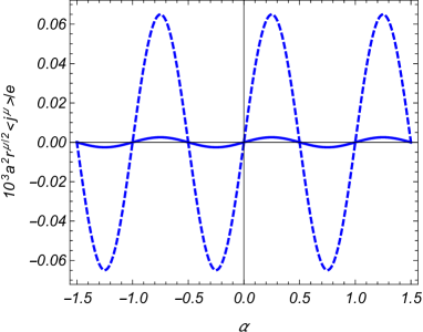
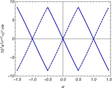
Figure 2: The dependence of the charge (full curves) and current (dashed curves) densities on the parameter $\alpha$ for the field with $s=1$. The graphs are plotted for $q=1.5$, $ma=0.5$, $b/a=4$, $r/a=2$. For the left panel $\lambda_{a}=\lambda_{b}=1$ and for the right one $\lambda_{a}=-\lambda_{b}=1$.

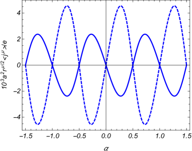
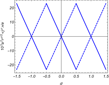
Figure 3: The same as in figure 2 for the fermionic field with $s=-1$.

Now we turn to the investigation of the radial dependence for the VEVs. In figure 4 the charge (left panel) and current (right panel) densities are depicted as functions of $r/a$ for a massless field and and boundary conditions with $\lambda_{a}=\lambda_{b}=1$. The graphs are plotted for $b/a=8$, $\alpha_{0}=1/4$, and the numbers near the curves correspond to the values of the parameter $q$. The curve for $q=1$ corresponds to a planar ring. As seen, the presence of the angle deficit may essentially increase both the charge and current densities. For the example presented in figure 4 the ratio $\langle j^{0}\rangle/e$ is negative near the inner edge and positive near the outer edge. The ratio $\langle j_{\phi}\rangle/e$ is positive.

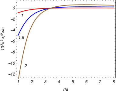
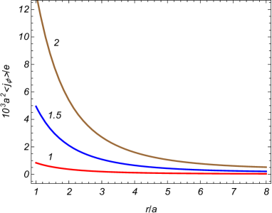
Figure 4: Charge and current densities versus $r/a$ for a massless fermionic field. The graphs are plotted for $b/a=8$, $\alpha_{0}=1/4$, $(s,\lambda_{a},\lambda_{b})=(1,1,1)$ and for different values of the parameter $q$ (numbers near the curves).

It is of interest to investigate the dependence of the VEVs on the values of the parameters $(s,\lambda_{a},\lambda_{b})$. Figures 5 and 6 display the radial dependence of the charge and current densities for different sets $(s,\lambda_{a},\lambda_{b})$ in the case of a massive field with the mass corresponding to $ma=0.5$. The graphs are plotted for $q=1.5$, $b/a=8$, $\alpha_{0}=1/4$. The curves with $\mu=0$ correspond to the charge density $\langle j^{0}\rangle$ and the curves $\mu=2$ correspond to the physical azimuthal component $\langle j_{\phi}\rangle=r\langle j^{2}\rangle$ of the current density. Figure 5 corresponds to fields with $(s,\lambda_{a},\lambda_{b})=(1,1,1)$ (left panel) and $(s,\lambda_{a},\lambda_{b})=(1,1,-1)$ (right panel). In figure 6, $(s,\lambda_{a},\lambda_{b})=(-1,1,1)$ for the left panel and $(s,\lambda_{a},\lambda_{b})=(-1,1,-1)$ for the right panel. The graphs for other sets of the parameters $(s,\lambda_{a},\lambda_{b})$ are obtained from the ones depicted in figures 5 and 6 by taking into account that under the reflection $(s,\lambda_{a},\lambda_{b})\rightarrow(-s,-\lambda_{a},-\lambda_{b})$ the charge density is an odd function and the current density is an even function. As seen, the charge and current densities are mainly located near the edges, inner or outer. The numerical data confirm the relations (3.5) between the charge and current densities on the edges of the ring. An important point to mention here is that the VEVs of the charge and current densities are finite on the edges of ring. This is not the case, for example, for the fermion condensate or for the VEV of the energy-momentum tensor.

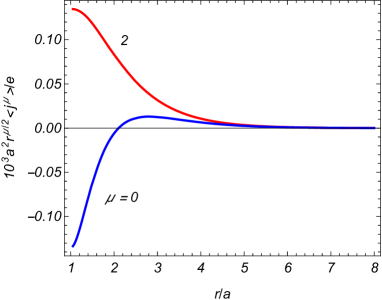
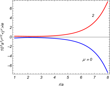
Figure 5: Charge ($\mu=0$) and current ($\mu=2$) densities as functions of the radial coordinate for a massive fermionic field. The graphs are plotted for $ma=0.5$, $b/a=8$, $\alpha_{0}=1/4$. The left and right panels correspond to the sets $(s,\lambda_{a},\lambda_{b})=(1,1,1)$ and $(s,\lambda_{a},\lambda_{b})=(1,1,-1)$, respectively.

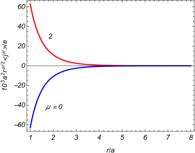
Figure 6: The same as in figure 5 for the sets $(s,\lambda_{a},\lambda_{b})=(-1,1,1)$ (left panel) and $(s,\lambda_{a},\lambda_{b})=(-1,1,-1)$ (right panel).

Comparing the left panel in figure 5 with the graphs in figure 4, we see that for a massive field the VEVs are essentially smaller. This can be not the case for other sets of the parameters $(s,\lambda_{a},\lambda_{b})$. In order to see the dependence of the VEVs on the field mass, in figure 7 we plot the charge and current densities as functions of $ma$ for fixed values $b/a=8$, $r/a=2$, $\alpha_{0}=1/4$ and for the field with $s=1$. The numbers near the curves are the values for $q$. The same graphs for the field with $s=-1$ are presented in figure 8. As the numerical results show, the dependence on the mass is essentially different for the cases $s=1$ and $s=-1$. For the parameters corresponding to 7 the VEVs decrease (by modulus) with increasing mass. For the example corresponding to figure 8 both the charge and current densities increase by modulus with initial increase of the mass and take their maximal or minimal values for some intermediate value of $ma$. The further increase of the mass, as expected, leads to the suppression of the VEVs.

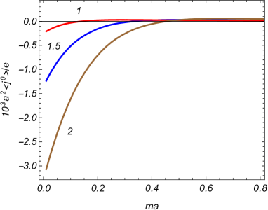
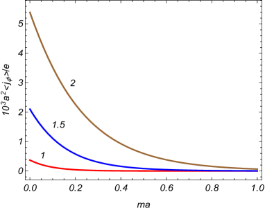
Figure 7: Charge and current densities as functions of the mass for $b/a=8$, $\alpha_{0}=1/4$, $r/a=2$, $(s,\lambda_{a},\lambda_{b})=(1,1,1)$. The numbers near the curves are the corresponding values of $q$.

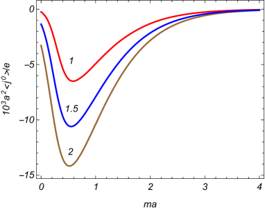
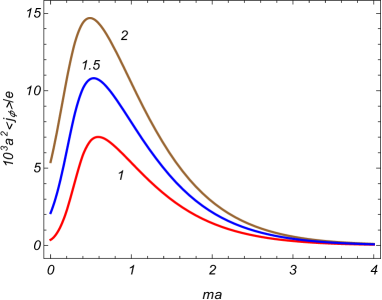
Figure 8: The same as in figure 7 for the field with $s=-1$.

5 VEVs in parity and time-reversal invariant models and applications to graphitic cones

5.1 VEVs for two irreducible representations of the Clifford algebra

The fermionic field we have considered lives in two-dimensional space. In even number of spatial dimensions there are two inequivalent irreducible representations of the Clifford algebra. In this section it will be shown how the VEVs of the charge and current densities are obtained from the results given above for the fields realizing those representations. We will distinguish the different representations by the parameter $s$ taking the values $-1$ and $+1$ (as it will be seen below it coincides with the parameter $s$ we introduced before in front of the mass term in the Dirac equation (2.2)). The corresponding sets of the $2\times 2$ Dirac matrices will be denoted by $\gamma_{(s)}^{\mu}=(\gamma^{0},\gamma^{1},\gamma_{(s)}^{2})$ and the related fields by $\psi_{(s)}(x)$. In the geometry described by the line element (2.1) the two inequivalent representations of the matrix $\gamma_{(s)}^{2}$ can be taken as $\gamma_{(s)}^{2}=-is\gamma^{0}\gamma^{1}/r$. For $s=+1$ the set $\gamma_{(s)}^{\mu}$ coincides with (2.3) used in the calculations above, $\gamma_{(+1)}^{\mu}=\gamma^{\mu}$. For the Lagrangian density corresponding to the fields $\psi_{(s)}(x)$ one has $L_{s}=\bar{\psi}_{(s)}(i\gamma_{(s)}^{\mu}D_{\mu}-m_{(s)})\psi_{(s)}$, where the mass for different representations, in general, can be different. The current densities of the fields are given by the standard formula $j_{(s)}^{\mu}=e\bar{\psi}_{(s)}\gamma_{(s)}^{\mu}\psi_{(s)}$. The boundary conditions on the edges we will take again in the form (2.4):

$$\left(1+i\lambda_{r}^{(s)}n_{\mu}\gamma_{(s)}^{\mu}\right)\psi_{(s)}(x)=0,\;r=a,b.$$ (5.1)

Here, the parameters $\lambda_{r}^{(s)}$ also can be different for separate representations.

Comparing with the discussion above, we see that for $\lambda_{r}^{(+1)}=\lambda_{r}$ the field equation and the boundary conditions for the field $\psi_{(+1)}(x)$ are the same as those for the field $\psi(x)$ with $s=1$ and $m=m_{(+1)}$, discussed in the previous sections. Hence, the expressions of the VEVs of the charge and current densities for $\psi_{(+1)}(x)$ coincide with those given above. In order to find the VEVs for the field $\psi_{(-1)}(x)$, we introduce a new field $\psi_{(-1)}^{\prime}$ according to $\psi_{(-1)}^{\prime}=\gamma^{0}\gamma^{1}\psi_{(-1)}$ with the inverse transformation $\psi_{(-1)}=\gamma^{0}\gamma^{1}\psi_{(-1)}^{\prime}$. The Lagrangian density is written as $L_{-1}=\bar{\psi}_{(-1)}^{\prime}(i\gamma^{\mu}D_{\mu}+m_{(-1)})\psi_{(-1)}^{\prime}$ with the gamma matrices $\gamma^{\mu}=\gamma_{(+1)}^{\mu}$ and for the current density we get $j_{(-1)}^{\mu}=e\bar{\psi}_{(-1)}^{\prime}\gamma^{\mu}\psi_{(-1)}^{\prime}$. As seen, in terms of the new field the mass term in the Lagrangian density reversed the sign. Substituting $\psi_{(-1)}=\gamma^{0}\gamma^{1}\psi_{(-1)}^{\prime}$ in the boundary condition (5.1) for $s=-1$, we get the corresponding condition for the primed field $\psi_{(-1)}^{\prime}(x)$:

$$\left(1-i\lambda_{r}^{(-1)}n_{\mu}\gamma^{\mu}\right)\psi_{(-1)}^{\prime}=0,$$ (5.2)

for $r=a,b$. From these considerations it follows that the charge and current densities for the field $\psi_{(-1)}(x)$ are obtained from the expressions given above taking $s=-1$ and $\lambda_{r}=-\lambda_{r}^{(-1)}$.

5.2 Charge and current densities in parity and time-reversal symmetric models

In two spatial dimensions, the mass term in the Lagrangian density for a two-component fermionic field $\psi(x)$ is not invariant under the parity ($P$) and time-reversal ($T$) transformations. In the absence of magnetic fields, $P$- and $T$-symmetric models can be constructed combining two fields realizing different irreducible representations of the Clifford algebra and having the same mass. In accordance with the consideration of the previous subsection, the Lagrangian density for this set of fields, denoted as before by $\psi_{(s)}$, $s=\pm 1$, is written in two equivalent forms

$$L = \sum_{s=\pm 1}\bar{\psi}_{(s)}(i\gamma_{(s)}^{\mu}D_{\mu}-m)\psi_{(s)}$$ (5.3)

$$= \sum_{s=\pm 1}\bar{\psi}_{(s)}^{\prime}(i\gamma^{\mu}D_{\mu}-sm)\psi_{(s)}^{\prime},$$

where $\psi_{(+1)}^{\prime}=\psi_{(+1)}$ and $\psi_{(-1)}^{\prime}=\gamma^{0}\gamma^{1}\psi_{(-1)}^{\prime}$. The total current density is given by the formula $J^{\mu}=e\sum_{s=\pm 1}\bar{\psi}_{(s)}\gamma_{(s)}^{\mu}\psi_{(s)}$ or by $J^{\mu}=e\sum_{s=\pm 1}\bar{\psi}_{(s)}^{\prime}\gamma^{\mu}\psi_{(s)}^{\prime}$. The separate fields obey the boundary conditions (5.1) or the conditions $\left(1+is\lambda_{r}^{(s)}n_{\mu}\gamma^{\mu}\right)\psi_{(s)}^{\prime}(x)=0$ in terms of the primed fields. Note that because of the appearance of the factor $s$ in front of the term with the normal to the boundary, the fields $\psi_{(+1)}^{\prime}$ and $\psi_{(-1)}^{\prime}$ obey different boundary conditions if the fields $\psi_{(+1)}$ and $\psi_{(-1)}$ are constrained by the same boundary conditions and vice versa.

We can combine the two-component fields $\psi_{(s)}(x)$ in a single 4-component spinor field $\Psi=(\psi_{(+1)},\psi_{(-1)})^{T}$ with the Lagrangian density

$$L=\bar{\Psi}(i\gamma_{(4)}^{\mu}D_{\mu}-m)\Psi,$$ (5.4)

where the $4\times 4$ Dirac matrices are given by $\gamma_{(4)}^{\mu}=I\otimes\gamma^{\mu}$ for $\mu=0,1$, and $\gamma_{(4)}^{2}=\sigma_{3}\otimes\gamma^{2}$ with $\sigma_{3}$ being the Pauli matrix. For the corresponding current density one has the standard expression $J^{\mu}=e\bar{\Psi}(x)\gamma_{(4)}^{\mu}\Psi(x)$. The boundary conditions on the edges $r=a,b$ are rewritten as

$$\left(1+i\Lambda_{r}n_{\mu}\gamma_{(4)}^{\mu}\right)\Psi(x)=0,$$ (5.5)

with $\Lambda_{r}=\mathrm{diag}(\lambda_{r}^{(+1)},\lambda_{r}^{(-1)})$. Alternatively, we can introduce the spinor $\Psi^{\prime}=(\psi_{(+1)}^{\prime},\psi_{(-1)}^{\prime})^{T}$ and the set of gamma matrices $\gamma_{(4)}^{\prime\mu}=\sigma_{3}\otimes\gamma^{\mu}$. For the corresponding Lagrangian density one gets $L=\bar{\Psi}^{\prime}(i\gamma_{(4)}^{\prime\mu}D_{\mu}-m)\Psi^{\prime}$ and for the current density operator $J^{\mu}=e\bar{\Psi}^{\prime}(x)\gamma_{(4)}^{\mu}\Psi^{\prime}(x)$. Now the boundary conditions take the form $\left(1+i\Lambda_{r}n_{\mu}\gamma_{(4)}^{\prime\mu}\right)\Psi^{\prime}(x)=0$. The latter has the same form as (5.5), though with different representation of the gamma matrices.

For $\lambda_{u}^{(+1)}=\lambda_{u}^{(-1)}$, $u=a,b$, the fields $\psi_{(+1)}$ and $\psi_{(-1)}$ in the Lagrangian density (5.3) obey the same boundary conditions. In this case the boundary condition for the transformed field $\psi_{(-1)}^{\prime}$ differs from the condition for the field $\psi_{(+1)}^{\prime}=\psi_{(+1)}$ by the sign of the term containing the normal to the boundary. As it has been shown above, the charge density is an odd function under the replacement $(s,\lambda_{u})\rightarrow(-s,-\lambda_{u})$, whereas the azimuthal current density is an even function. From here we conclude that in the model involving two fields $\psi_{(+1)}$ and $\psi_{(-1)}$ with the same masses and the phases in the periodicity condition (2.6), obeying the boundary conditions (5.1) with $\lambda_{u}^{(+1)}=\lambda_{u}^{(-1)}$, the VEV of the total charge density vanishes, $\langle J^{0}\rangle=0$, and for the VEV of the total current density one gets $\langle J^{2}\rangle=2\langle j^{2}\rangle$, where $\langle j^{2}\rangle$ is given by (3.23) with $\mu=2$ and with $s=1$, $\lambda_{u}=\lambda_{u}^{(+1)}$.

In models with two fields $\psi_{(+1)}$ and $\psi_{(-1)}$, realizing inequivalent irreducible representations of the Clifford algebra, a nonzero vacuum charge density may appear if the corresponding boundary conditions are different ($\lambda_{u}^{(+1)}\neq\lambda_{u}^{(-1)}$) or the masses for the fields differ. However, note that the difference in the masses will break the parity and time-reversal symmetry of the model. Another possibility for the appearance of the nonzero charge density is realized in models with different phases in the periodicity conditions (2.6) for the fields $\psi_{(+1)}$ and $\psi_{(-1)}$. The latter type of situation takes place in semiconducting carbon nanotubes where the fields under consideration describe the electronic subsystem of graphene tubes.

5.3 Current density in graphitic cones

Among important realizations of 2D fermionic models is graphene. The existence of various classes of graphene allotropes, like carbon nanotubes, fullerens, graphitic cones, nanoloops and nanohorns, makes graphene an exciting arena for the investigation of the effects of the geometry, topology and boundaries on the properties of a quantum fermionic field. Recently, a number of mechanisms have been suggested (see, for example, [46]) to generate effective curved background geometries for Dirac fermions in graphene. In particular, they include various types of external fields, lattice deformations, and local variations of the Fermi velocity. The advantage of these graphene based artificial systems in modelling the influence of the gravity on quantum matter is that one can tune in a controlled manner the geometrical characteristics of the background spacetime.

In the long wavelength approximation, the effective field theory for the electronic subsystem in graphene is formulated in terms of 4-component spinors $\Psi_{S}=(\psi_{+,AS},\psi_{+,BS},\psi_{-,AS},\psi_{-,BS})^{T}$, where $S=\pm 1$ corresponds to the spin degree of freedom. It is decomposed into two 2-component spinors, $\psi_{+}=(\psi_{+,AS},\psi_{+,BS})$ and $\psi_{-}=(\psi_{-,AS},\psi_{-,BS})$, corresponding to two inequivalent corner points $\mathbf{K}_{+}$ and $\mathbf{K}_{-}$ of the hexagonal Brillouin zone of graphene. These two valleys are related by the time-reversal symmetry. The separate components $\psi_{\pm,AS}$ and $\psi_{\pm,BS}$ give the amplitude of the electron wave function on the triangular sublattices $A$ and $B$ of the graphene hexagonal lattice. In the standard units with the speed of light $c$ and the Planck constant $\hbar$, the Lagrangian density in the effective field theory is presented as

$$L_{\mathrm{g}}=\sum_{S=\pm 1}\bar{\Psi}_{S}[i\hbar\gamma_{(4)}^{0}\partial_{t}+i\hbar v_{F}\gamma_{(4)}^{l}(\nabla_{l}+ieA_{l}/\hbar c)-\Delta]\Psi_{S},$$ (5.6)

where $l=1,2$, $e$ is the electron charge and $v_{F}\approx 7.9\times 10^{7}$ cm/s is the Fermi velocity for electrons. The energy gap $\Delta$, introduced in (5.6), is related to the Dirac mass $m$ by $\Delta=mv_{F}^{2}$. A number of mechanisms has been considered in the literature for the generation of the energy gap in the range $1\,\mathrm{meV}\lesssim\Delta\lesssim 1\,\mathrm{eV}$ (see, for example, [5] and references therein). The energy scale in the model is determined by the parameter $\gamma_{F}=$ $\hbar v_{F}/a_{0}\approx 2.51\,\mathrm{eV}$, where $a_{0}\approx 1.42$ Å is the inter-atomic spacing of graphene honeycomb lattice. For the Compton wavelength related to the energy gap one has $a_{C}=\hbar v_{F}/\Delta$. For a given $S$, the charge density corresponding to the Lagrangian (5.6) is given by $J^{0}=e\bar{\Psi}_{S}(x)\gamma_{(4)}^{0}\Psi_{S}(x)$ and for the current density we get $J^{\mu}=ev_{F}\bar{\Psi}_{S}(x)\gamma_{(4)}^{\mu}\Psi_{S}(x)$, $\mu=1,2$.

The separate parts in (5.6) for given $S$ are the analog of the Lagrangian density (5.4) we have discussed before. The two-component fields $\psi_{(+1)}$ and $\psi_{(-1)}$ correspond to the fields $\psi_{+}$ and $\psi_{-}$. Hence, the parameter $s$ in the discussion above enumerates the valley degrees of freedom in graphene. On the base of this analogy, we can apply the formulas for the charge and current densities given above to graphene conical ribbons with the edges $r=a$ and $r=b$. The graphene nanocones have attracted considerable attention due to their potential applications such as probes for scanning probe microscopy, electron emitters, tweezers for nanomanipulation, energy storage, gas sensors, and biosensors. In the problem under consideration the separate parts with $S=\pm 1$ give the same contributions to the VEVs and we can consider the VEVs for a given spin degree of freedom omitting the index $S$. The total VEVs are obtained with an additional factor 2. As it has been already mentioned in Introduction, for the opening angle in graphitic cones one has $\phi_{0}=2\pi(1-n_{c}/6)$ with $n_{c}=1,2,\ldots,5$ being the number of the removed sectors from a planar graphene sheet. The analog of the quasiperiodicity condition (2.6) in graphene cones has been discussed in [24, 26, 28, 31]. For graphene cones with odd values of $n_{c}$ it mixes the valley indices through the factor $e^{-i\pi n_{c}\tau_{2}/2}$, where the Pauli matrix $\tau_{2}$ acts on those indices. The corresponding condition can be diagonalized by a unitary transformation that diagonalizes the matrix $\tau_{2}$. For even values of $n_{c}$ the spinors corresponding to different valleys are not entwined and an additional diagonalization is not required. By taking into account that only the fractional part of the parameter $\chi$ is relevant in the evaluation of the VEVs, it can be seen that two inequivalent values of the parameter $\chi$ realized in graphitic cones correspond to $\chi=\pm 1/3$. Note that the same inequivalent values of the periodicity phase are realized in semiconducting carbon nanotubes (in metallic nanotubes $\chi=0$). The fermionic current density in cylindrical and toroidal carbon tubes has been investigated in [15, 19].

For a given spin $S$, the ground state charge and current densities in graphitic cones are obtained from the results in section 3 in accordance of the procedure described in the previous subsection, adding an additional factor $v_{F}$ for the azimuthal current density. Translating the results given above to graphene made structures it is convenient to make the replacements $mu\rightarrow u/a_{C}$, $u=a,b,r$, in the corresponding formulas. If the energy gap is the same for both the valleys, the net charge density vanishes as a consequence of the cancellation between the contributions from different valleys. However, there exist gap generations mechanisms in graphene breaking the valley symmetry (for example, chemical doping) and one can have a situation with different masses for the fields $\psi_{+}$ and $\psi_{-}$. In this case there is no cancellation of the corresponding contributions to the charge density. Note that the magnetic flux induced currents in planar graphene rings have been investigated in [37, 47]. Based on the concept of branes, a model for the emergence of current density in graphene in the presence of defects has been recently discussed in [48].

6 Conclusion

The notion of vacuum in quantum field theory has a global nature and its properties are sensitive to both the local and global characteristics of the background spacetime. In the present paper we have investigated the combined effects of boundaries, topology and of the magnetic flux on the ground state mean charge and current densities for a fermionic field in two-dimensional conical rings with arbitrary values of the angle deficit. The boundary conditions for the field operator on the ring edges are specified by the set of parameters $(\lambda_{a},\lambda_{b})$. In the special case $(1,1)$ they are reduced to the standard MIT bag boundary condition (infinite mass boundary condition in the context of 2D fermionic systems). An additional parameter $s$ in front of the mass term in the Dirac equation corresponds to two inequivalent irreducible representations of the Clifford algebra in (2+1)-dimensional spacetime. The fermionic mode functions are presented as (2.10), where the allowed values of the radial quantum number depend on the specific boundary condition and are roots of equation (2.14). For whole family of boundary conditions, we have considered, the vacuum state is stable and for all the roots $\gamma^{2}\geq-m^{2}$. For fields with $(s,\lambda_{a},\lambda_{b})=\left(\pm 1,\pm 1,\pm 1\right)$ all the eigenvalues for $\gamma$ are real. In the remaining cases, depending on $b/a$ and $ma$, purely imaginary eigenvalues $\gamma=i\eta/a$, $0<\eta<ma$, may appear corresponding to bound states. For half-integer values of the parameter $\alpha$ from (2.15) and under the condition $\lambda_{a}=-\lambda_{b}$ there is also a zero mode with the value of the total angular momentum $j=-\alpha$.

The VEVs of the charge and current densities are evaluated by using the corresponding mode sums over the bilinear products of the mode functions. The VEV for the radial current vanishes and the contribution of the modes with positive $\gamma$ to the charge and azimuthal current densities is presented as (3.1). In the presence of the bound state or the zero mode, the corresponding contributions, given by (A.8) and (B.8), should be added to (3.1). The charge and current densities on the ring edges are connected by simple relation (3.5) that is valid for whole family of boundary conditions. For half-integer values of $\alpha$ the charge and current densities vanish for the boundary conditions with $\lambda_{a}=\lambda_{b}$. For the conditions with $\lambda_{a}=-\lambda_{b}$ the only nonzero contribution comes from the zero mode. In the latter case the charge and current densities are discontinuous functions of $\alpha$ (in particular, of the magnetic flux enclosed by the ring) at half-integer values of that parameter.

In the representation (3.1) the summation goes over the eigenvalues for $\gamma$ given implicitly, as roots of equation (2.14). The explicit knowledge of those roots is not required if we apply the summation formula (3.6) to the corresponding series. In the presence of the bound states an additional term in the form (A.12) should be added to the right-hand side of (3.6). We have shown that the additional term exactly cancels the contribution coming from the bound states and the integral representation (3.8) is valid for all the sets of parameters $(s,\lambda_{a},\lambda_{b})$. The first term in the right-hand side of (3.8) corresponds to the VEV in the conical geometry with a single boundary at $r=a$ and the last term is interpreted as the contribution induced by the second edge at $r=b$. The former part is further decomposed as (3.14) with the boundary-free and edge induced contributions, given by (3.19) and (3.17), respectively. An alternative representation, where the part corresponding to the problem inside a single circular boundary is extracted, is given by (3.28). As a general rule, the modulus of both the charge and current densities increases with increasing planar angle deficit (with increasing $q$). Depending on the boundary condition, determined by the set $(\lambda_{a},\lambda_{b})$, the charge and current densities are mainly located near the inner or outer edge (see figures 4-6). We have demonstrated that the behavior of the VEVs as functions of the mass can be essentially different for fields with $s=+1$ and $s=-1$. In the former case and for the boundary condition with $(\lambda_{a},\lambda_{b})=(1,1)$ the absolute values of the charge and current densities decrease with increase of the field mass. In the case $s=-1$ and for the same boundary condition, the absolute values for both the charge and current densities increase with initial increase of the mass. After taking the maximum value, as expected, they tend to zero for large masses.

It is well known that in two spatial dimensions the fermionic mass term breaks both the parity and time reversal invariances. $P$- and $T$-symmetric fermionic models are constructed considering the set of two fields, $\psi_{(+1)}$ and $\psi_{(-1)}$, with the same masses realizing two inequivalent irreducible representations of the Clifford algebra. The VEVs of the charge and current densities for the field corresponding to the second representation and obeying the boundary condition (5.1) are obtained from the formulas in section 3.1 with $s=-1$ and $\lambda_{u}=-\lambda_{u}^{(-1)}$, $u=a,b$. If in addition to the masses, the phases in the periodicity condition along the azimuthal direction and the boundary conditions on the edges for the fields $\psi_{(+1)}$ and $\psi_{(-1)}$ are the same then the total charge density vanishes, whereas the total current density doubles. In the effective low-energy theory for electronic subsystem of graphene, the fields $\psi_{(+1)}$ and $\psi_{(-1)}$ correspond to two inequivalent points of the Brillouin zone (valley degrees of freedom) and the results obtained in the present paper can be applied for the investigation of the charge and current densities induced by Aharonov-Bohm magnetic flux in graphitic cones. Two inequivalent values of the phase $2\pi\chi$ realized in graphitic cones correspond to $\pm 2\pi/3$ and for the parameter $q$ one has $q=1/(1-n_{c}/6)$. It is of interest to note that the valley-dependent gap generation mechanisms (for a recent discussion see [49] and references therein) create different masses for the fields $\psi_{(+1)}$ and $\psi_{(-1)}$ and, as a result of that, the nonzero net charge density appears. This breaks the time-reversal symmetry.

Appendix A Contribution of the bound states

In addition to the infinite set of positive modes $\gamma=\gamma_{l}$, depending on the parameters of the model, the equation (2.14) for the eigenmodes may have purely imaginary solutions $\gamma a=i\eta$, $\eta>0$. For the modes with $\eta>ma$ the corresponding energy is imaginary and the presence of these modes would signal about the instability of the vacuum state. In the case $\eta>ma$ the equation determining the modes is given by

$$K_{n_{p}}^{(a)}\left(\eta\right)I_{n_{p}}^{(b)}\left(\eta b/a\right)-I_{n_{p}}^{(a)}(\eta)K_{n_{p}}^{(b)}(\eta b/a)=0.$$ (A.1)

The left-hand side is a complex function and the real and imaginary parts should be separately zero. Introducing the function

$$B_{\mu,\nu}(x,y)=I_{\mu}(x)K_{\nu}(y)-(-1)^{\mu-\nu}K_{\mu}(x)I_{\nu}(y),$$ (A.2)

from those conditions it follows that we should have

$$B_{n_{p}+1,n_{p}+1}\left(\eta,\eta b/a\right)=\lambda_{a}\lambda_{b}B_{n_{p},n_{p}}\left(\eta,\eta b/a\right).$$ (A.3)

By taking into account that $B_{\nu,\nu}\left(\eta,\eta b/a\right)<0$ for $\nu\geq-1/2$, we see that the equation (A.3) has no solutions for $\lambda_{a}\lambda_{b}<0$. For $\lambda_{a}\lambda_{b}>0$, noting that $B_{\nu+1,\nu+1}\left(\eta,\eta b/a\right)<B_{\nu,\nu}\left(\eta,\eta b/a\right)$ for $\nu>-1/2$, again, (A.3) has no solutions. Hence, for all the values of the parameters $s,\lambda_{a},\lambda_{b}$ there are no modes with $\eta>ma$ and the vacuum state is stable.

Now we turn to the modes $\gamma a=i\eta$, $\eta>0$, with $\eta<ma$. These modes correspond to bound states. They are determined by the equation (2.14) with $\gamma a=i\eta$. Introducing the modified Bessel functions it is written in the form

$$G_{\beta_{j}}(\eta,\eta b/a)\equiv I_{\beta_{j}}^{(a)}\left(\eta\right)K_{\beta_{j}}^{(b)}\left(\eta b/a\right)-I_{\beta_{j}}^{(b)}\left(\eta b/a\right)K_{\beta_{j}}^{(a)}\left(\eta\right)=0,$$ (A.4)

where the functions $f_{\beta_{j}}^{(u)}(z)$ with $f=I,K$ are defined by (3.11) with the replacement

$$i\sqrt{z^{2}-m_{u}^{2}}\rightarrow\kappa\sqrt{m_{u}^{2}-z^{2}}.$$ (A.5)

This replacement is understood also in the following formulas in this appendix.

If we write the roots of (A.4) as functions of the parameters, $\eta=\eta(b/a,s,\lambda_{u},j,\alpha_{0},\kappa)$, then the solutions for different sets of the parameters in the arguments are connected by the same relations as those for the modes $z_{l}$ (see the paragraph after formula (2.15)). For all values of the ratio $b/a$ the bound states are absent in the cases $(s,\lambda_{a},\lambda_{b})=(\pm 1,\pm 1,\pm 1)$. For the remaining sets, depending on the values of the parameters, we have the following two possibilities: (i) the bound states are present for all values of the ratio $b/a$ or (ii) they appear started from some critical value of that parameter, denoted here as $(b/a)_{\mathrm{c}}$. The numerical analysis has shown the following features. If there is no bound state for some $j=j_{(\mathrm{b})}$, then there is no bound state for angular quantum numbers with $|j|>|j_{(\mathrm{b})}|$. The critical values of $b/a$ for the appearance of the bound states increase with decreasing $ma$. The critical value $(b/a)_{\mathrm{c}}$ also increases with increasing $q$. The latter means that we can have a situation when the bound state is present in a planar ring and is absent in the conical ring for the same values of the other parameters. For example, for $\kappa=+$, $ma=0.5$, $\alpha_{0}=1/4$ and $(s,\lambda_{a},\lambda_{b})=(-1,1,1)$ for a planar ring ($q=1$) one has $(b/a)_{\mathrm{c}}\approx 3.13,4.5$ for $j=1/2,3/2$, respectively. For a conical ring we get $(b/a)_{\mathrm{c}}\approx 3.6,6.22$ for $j=1/2,3/2$. For $(s,\lambda_{a},\lambda_{b})=(-1,1,1)$ and for the same values of the other parameters the bound states are present only for $q=1$, $j=1/2$ with the critical value $(b/a)_{\mathrm{c}}\approx 4.88$ and and there are no bound states for $q=1.5$.

In the limit $b/a\rightarrow\infty$ the equation for the bound states is reduced to $K_{\beta_{j}}^{(a)}\left(\eta\right)=0$. The latter is the equation for the bound states in a conical space with a single boundary at $r=a$ and has no solutions for $s\lambda_{a}>0$. In this case, in the limit $b/a\rightarrow\infty$ the possible bound states determined from (A.4) tend to $ma$. If there is a bound state in the geometry of a single boundary, then in the limit $b/a\rightarrow\infty$ the corresponding bound state for a conical ring (with the same values for the set $(s,\lambda_{a},j,\alpha_{0},\kappa)$) tends to the limiting value different from $ma$. These two situations are illustrated in figure 9, where we have plotted the radial quantum number $\eta$ for the bound states as a function of the ratio $b/a$ for $(s,\lambda_{a},\lambda_{b})=(-1,-1,1)$ (left panel) and $(s,\lambda_{a},\lambda_{b})=(1,-1,-1)$ (right panel). The graphs are plotted for $\kappa=+$, $ma=3$ and $\alpha_{0}=1/4$ and the numbers near the curves are the values of $j$. The dashed and full curves correspond to $q=1$ (planar ring) and $q=1.5$, respectively. For the left panel $s\lambda_{a}>0$ and there is no bound state in a conical geometry with a single boundary, $r\geq a$. In this case the bound states tend to $ma$ for $b/a\gg 1$. For the right panel the equation $K_{\beta_{j}}^{(a)}\left(\eta\right)=0$ has a solution and it is the limiting value of the bound state when $b/a\rightarrow\infty$. On the right panel we also see that the bound states appear only started from some critical value of $b/a$. By using the relations between the bound states for different sets of the parameters, we see that the graphs in figure 9 also present the locations of the bound states for the set $(-j,-\alpha_{0},-\kappa)$ or for the set $(-s,-\lambda_{u},-\kappa)$ with the same values of the remaining parameters.

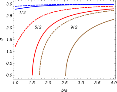
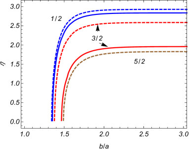
Figure 9: The values of $\eta$ for bound states versus the ratio $b/a$. The numbers near the curves are the values of the quantum number $j$. The left and right panels are plotted for the values of the parameters $(s,\lambda_{a},\lambda_{b})=(-1,1,1)$ and $(s,\lambda_{a},\lambda_{b})=(-1,-1,1)$, respectively. The full and dashed curves correspond to the cases $q=1.5$ and $q=1$. For the other parameters we have taken $\alpha_{0}=1/4$ and $ma=3$.

It is of interest to compare the number of the positive and negative energy bound states for given values of the other parameters. In figure 10 the bound states are presented as functions of $b/a$ for $q=1.5$, $\alpha_{0}=1/4$, $ma=1$, and for the set $(s,\lambda_{a},\lambda_{b})=(1,-1,-1)$. The numbers near the curves are the values of the total angular momentum $j$. The full and dashed curves correspond to the positive ($\kappa=+$) and negative ($\kappa=-$) energy modes.

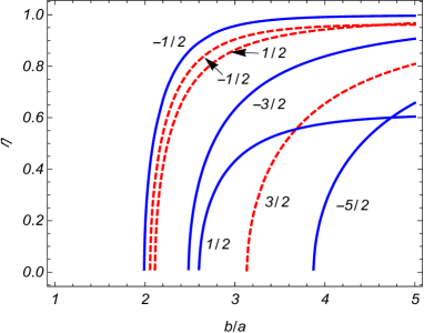
Figure 10: The values of $\eta$ corresponding to the bound states versus $b/a$ for $q=1.5$, $\alpha_{0}=1/4$, $ma=1$, $(s,\lambda_{a},\lambda_{b})=(1,-1,-1)$. The full and dashed curves correspond to positive and negative energy states and the numbers near the curves are the values of $j$.

If bound states are present their contribution should be added to the right-hand side of (3.1). The corresponding mode functions are given by

$$\psi_{\sigma}^{(\mathrm{b},\kappa)}(x)=C_{\kappa}^{(b)}e^{iq(j+\chi)\phi-\kappa iEt}\left(\begin{array}[]{c}G_{\beta_{j},\beta_{j}}^{(a)}(\eta,\eta r/a)e^{-iq\phi/2}\\ -\frac{e^{iq\phi/2}\eta/a}{\kappa E+sm}G_{\beta_{j},\beta_{j}+\epsilon_{j}}^{(a)}(\eta,\eta r/a)\end{array}\right),$$ (A.6)

with the energy $E=\sqrt{m^{2}-\eta^{2}/a^{2}}$. Here the function $G_{\beta_{j},\mu}^{(u)}(x,y)$ is defined by (3.10) with $f_{\beta_{j}}^{(u)}(z)$ obtained from (3.11) by the replacement (A.5). From the condition (2.16) for the normalization coefficient we find

$$\left|C_{\kappa}^{(b)}\right|^{2}=\frac{q\eta^{2}}{4\pi a^{2}E}\left[B_{a}-\frac{B_{b}I_{\beta_{j}}^{(a)2}\left(\eta\right)}{I_{\beta_{j}}^{(b)2}\left(\eta b/a\right)}\right]^{-1},$$ (A.7)

where $B_{u}$ is defined in accordance with (2.19).

Substituting the mode functions into the mode sum (2.8) for the contribution of the bound states to the VEV $\langle j^{\mu}\rangle$ we get

$$\langle j^{\mu}\rangle_{(\mathrm{b})}=-\frac{eq}{8\pi}\sum_{j}\sum_{\kappa=\pm}\,\frac{\left(\kappa sm-E\right)w_{\mu,\beta_{j}}^{(\mathrm{b})}(\eta)/E}{B_{a}-B_{b}I_{\beta_{j}}^{(a)2}\left(\eta\right)/I_{\beta_{j}}^{(b)2}\left(\eta x\right)},$$ (A.8)

with $\mu=0,2$ and with the functions

$$w_{0,\beta_{j}}^{(\mathrm{b})}(\eta) = \left(sm+\kappa E\right)G_{\beta_{j},\beta_{j}}^{(a)2}(\eta,\eta r/a)+\left(sm-\kappa E\right)G_{\beta_{j},\beta_{j}+\epsilon_{j}}^{(a)2}(\eta,\eta r/a),$$

$$w_{2,\beta_{j}}^{(\mathrm{b})}(\eta) = -\frac{2\eta}{ar}G_{\beta_{j},\beta_{j}}^{(a)}(\eta,\eta r/a)G_{\beta_{j},\beta_{j}+\epsilon_{j}}^{(a)}(\eta,\eta r/a).$$ (A.9)

The total current density is the sum of the parts (3.1) and (A.8). On the edges of the ring one gets simplified expression for the charge density:

$$\langle j^{0}\rangle_{(\mathrm{b}),r=u}=-\frac{eq}{4\pi a^{2}}\sum_{j}\sum_{\kappa=\pm}\frac{\eta^{2}}{E}\,\frac{\kappa I_{\beta_{j}}^{(a)2}\left(\eta\right)/I_{\beta_{j}}^{(b)2}\left(\eta u/a\right)}{B_{a}-B_{b}I_{\beta_{j}}^{(a)2}\left(\eta\right)/I_{\beta_{j}}^{(b)2}\left(\eta b/a\right)},$$ (A.10)

where $u=a,b$. For the azimuthal current density on the edges we have the relation (3.5).

For the evaluation of the sum over $l$ in (3.1) we again can apply the Abel-Plana type formula (3.6). However, in the presence of the modes $\gamma a=i\eta$ the summation formula (3.6) is modified: an additional term appears in the right-hand side coming from the poles $z=\pm i\eta$. The derivation of the summation formula from the generalized Abel-Plana formula is similar to that for (3.6) presented in [43]. The difference is that now the function $g(z)$ in the generalized Abel-Plana formula has poles $z=\pm i\eta$ on the imaginary axis. In the corresponding integral these poles should be avoided by small semicircles in the right half plane with the centers at $z=i\eta$ and $z=-i\eta$. The contributions of the integrals over these semicircles are combined, up to the coefficient $-\pi^{2}/4$, as the term

$$i{{\frac{I_{\nu}^{(b)}(\eta b/a)}{I_{\nu}^{(a)}(\eta)}}}\frac{{{w(i\eta)}-w(-i\eta)}}{\partial_{z}G_{\beta_{j}}(z,zb/a)|_{z=\eta}}.$$ (A.11)

Now, the summation formula for the series over the positive roots $\gamma_{l}$ is obtained from (3.6) by adding to the right-hand side of that formula the term (A.11).

After the application of the summation formula (3.6) with the additional term (A.11) in the right-hand side, the contribution to the current density from the modes with $\gamma=\gamma_{l}$ is given by (3.8) plus the part coming from (A.11). By taking into account that $w_{\mu,\beta_{j}}(ze^{-\pi i/2})=-w_{\mu,\beta_{j}}(ze^{\pi i/2})$ for $z<m_{a}$, we can see that the additional term in the VEV $\langle j^{\mu}\rangle$ is presented as

$$\frac{qe}{4\pi a^{2}}\sum_{j}\sum_{\kappa=\pm}\,{{\frac{I_{\nu}^{(b)}(\eta b/a)}{I_{\nu}^{(a)}(\eta)}}}\frac{\eta w_{\mu,\beta_{j}}^{(\mathrm{b})}(\eta)/E}{\partial_{z}G_{\beta_{j}}(z,zb/a)|_{z=\eta}}.$$ (A.12)

By using the definition (A.4) and the fact that $z=\eta$ is the zero of the function $G_{\beta_{j}}(z,zb/a)$, one can show that the derivative in (A.12) is given by

$$\partial_{z}G_{\beta_{j}}(z,zb/a)|_{z=\eta}=\frac{2\kappa a^{-2}\eta}{sm-\kappa E}\left[B_{a}\frac{I_{\beta_{j}}^{(b)}\left(\eta b/a\right)}{I_{\beta_{j}}^{(a)}\left(\eta\right)}-B_{b}\frac{I_{\beta_{j}}^{(a)}\left(\eta\right)}{I_{\beta_{j}}^{(b)}\left(\eta b/a\right)}\right].$$ (A.13)

Substituting this into (A.12) we see that the contribution (A.12) is the same as (A.8) but with the opposite sign. From here we conclude that the contribution of the bound states to the total VEV $\langle j^{\mu}\rangle$ is cancelled by the contribution of the additional term (A.11) in the summation formula for the modes $\gamma_{l}$. Hence, all the representations for the charge and current densities given above, started from (3.8), are valid in the case of the presence of bound states as well.

Appendix B Special mode and its contribution to the VEVs

For half-integer values of the parameter $\alpha$ there is a special mode corresponding to $j=-\alpha$. For this mode the upper and lower components of the spinor are expressed in terms of the cylinder functions with the orders $\pm 1/2$ and the mode functions obeying the boundary condition (2.4) on the edge $r=a$ have the form

$$\psi_{(\mathrm{s})\sigma}^{(\kappa)}(x)=C_{(\mathrm{s})}\sqrt{\frac{E+\kappa sm}{\phi_{0}r\left(b-a\right)E}}e^{iq(\chi-\alpha-1/2)\phi-\kappa iEt}\left(\begin{array}[]{c}\cos\left[\gamma\left(r-a\right)+\gamma_{a}\right]\\ \frac{\gamma e^{iq\phi}}{\kappa E+sm}\sin\left[\gamma\left(r-a\right)+\gamma_{a}\right]\end{array}\right)\ ,$$ (B.1)

with $\gamma_{a}$ defined by the relations

$$\sin\gamma_{a}=-\sqrt{\frac{E+\kappa sm}{2E}},\;\cos\gamma_{a}=\kappa\lambda_{a}\sqrt{\frac{E-\kappa sm}{2E}}.$$ (B.2)

The coefficient is given by

$$C_{(\mathrm{s})}=\left\{1+\frac{\kappa sm}{2zE}\left[\sin\left(2z+2\gamma_{a}\right)+\kappa\lambda_{a}\frac{\gamma}{E}\right]\right\}^{-1/2},$$ (B.3)

with $z=\gamma(b-a)$. From the boundary condition (2.4) at $r=b$ we get the equation for the eigenvalues of $\gamma$:

$$\kappa\left(\lambda_{a}+\lambda_{b}\right)\left(\cos z+\lambda_{a}s\frac{m}{\gamma}\sin z\right)+\left(1-\lambda_{a}\lambda_{b}\right)\frac{E}{\gamma}\sin z=0.$$ (B.4)

The positive roots of this equation will be denoted by $\gamma=\gamma_{l}^{(\mathrm{s})}$, $l=1,2,3,\ldots$.

On the base of the modes (B.1), for the contribution of the special mode to the charge density one gets

$$\langle j^{\mu}\rangle_{(\mathrm{s})}=-\frac{e}{2\phi_{0}\left(b-a\right)r}\sum_{l=1}^{\infty}\sum_{\kappa=-,+}\kappa C_{(\mathrm{s})}^{2}w_{(\mathrm{s})\mu}(\gamma_{l}^{(\mathrm{s})}),$$ (B.5)

where

$$w_{(\mathrm{s})0}(\gamma) = 1+\frac{sm}{E^{2}}\left\{\lambda_{a}\gamma\sin\left[2\gamma\left(r-a\right)\right]-sm\cos\left[2\gamma\left(r-a\right)\right]\right\},$$

$$w_{(\mathrm{s})2}(\gamma) = -\frac{\gamma}{rE^{2}}\left\{sm\sin\left[2\gamma\left(r-a\right)\right]+\lambda_{a}\gamma\cos\left[2\gamma\left(r-a\right)\right]\right\}.$$ (B.6)

As it is seen from (B.4), for the specification of the eigenvalues $\gamma_{l}$ two cases should be considered separately.

In the case $\lambda_{b}=-\lambda_{a}$ the equation for $\gamma$ is reduced to $\sin[\gamma(b-a)]=0$ with the eigenvalues $\gamma_{l}^{(\mathrm{s})}=\pi l/(b-a)$, $l=1,2,\ldots$. For these modes $C_{(\mathrm{s})}^{2}=1$ and, hence, in (B.5) the factor $C_{(\mathrm{s})}^{2}w_{(\mathrm{s})\mu}(\gamma_{l}^{(\mathrm{s})})$ is the same for the positive and negative energy modes. Consequently, the contributions $\langle j^{\mu}\rangle_{(\mathrm{s})}$ for both the charge and current densities are zero because of the cancellation between the positive and negative energy modes.

For $j=-\alpha$ and $\lambda_{b}=-\lambda_{a}$, in addition to the modes with positive $\gamma$ there is a zero energy mode with $E=0$ and $\gamma=im$. The corresponding normalized mode function is given by

$$\psi_{(\mathrm{s})}^{(0)}=\frac{\sqrt{m/(\phi_{0}r)}e^{\lambda_{a}smr+iq\left(\chi-\alpha-1/2\right)\phi}}{\left[\lambda_{a}s\left(e^{2\lambda_{a}smb}-e^{2\lambda_{a}sma}\right)\right]^{1/2}}\left(\begin{array}[]{c}1\\ -\lambda_{a}e^{iq\phi}\end{array}\right),$$ (B.7)

and $\lambda_{b}=-\lambda_{a}$. For the contribution of this mode to the charge density we get

$$\langle j^{0}\rangle_{\mathrm{(s)}}^{(0)}=\pm\frac{e}{\phi_{0}r}\frac{\lambda_{a}sme^{2\lambda_{a}smr}}{e^{2\lambda_{a}smb}-e^{2\lambda_{a}sma}},$$ (B.8)

and for the azimuthal current density one has $\langle j^{2}\rangle_{\mathrm{(s)}}^{(0)}=-\lambda_{a}\langle j^{0}\rangle_{\mathrm{(s)}}^{(0)}/r$ for all values $a\leq r\leq b$. The reason for the appearance of two signs in the presence of the fermionic zero mode is the same as that discussed in [50]

In the case $\lambda_{b}=\lambda_{a}$, the boundary condition (B.4) leads to the equation

$$\cos z+(\lambda_{a}sm/\gamma)\sin z=0,$$ (B.9)

with $z=\gamma(b-a)$. It is the same for the positive and negative energy modes. Note that the equation (B.9) coincides with the eigenvalue equation for a finite length cylindrical tube (see [19] for the case $\lambda_{a}s=1$). For the solutions of (B.9) the expression for (B.3) is simplified to $C_{(\mathrm{s})}^{-2}=1-\sin\left(2z\right)/2z$ and, again, is the same for the modes $\kappa=+$ and $\kappa=-$. Hence, as in the previous case, the contributions of the positive and negative energy modes cancel each other in the VEVs (B.5).

Concluding the analysis in this section, for half-integer values of $\alpha$ the special mode with the angular momentum $j=-\alpha$ does not contribute to the VEVs of the charge and current densities in the case $\lambda_{b}=\lambda_{a}$. In the case $\lambda_{b}=-\lambda_{a}$ the only nonzero contributions come from the zero energy mode (B.7). For the charge density that contribution is given by (B.8).

References

- [1] N. Nagaosa, Quantum Field Theory in Condensed Matter Physics and Quantum Field Theory in Strongly Correlated Electronic Systems (Springer, Berlin, 1999).
- [2] G.V. Dunne, Topological Aspects of Low Dimensional Systems (Springer, Berlin, 1999).
- [3] E. Fradkin, Field Theory of Condensed Matter Systems (Cambridge University Press, Cambridge, 2013).
- [4] E.C. Marino, Quantum Field Theory Approach to Condensed Matter Physics (Cambridge University Press, Cambridge, 2017).
- [5] V.P. Gusynin, S.G. Sharapov, and J.P. Carbotte, Int. J. Mod. Phys. B 21, 4611 (2007).
- [6] A.H. Castro Neto, F. Guinea, N.M.R. Peres, K.S. Novoselov, and A.K. Geim, Rev. Mod. Phys. 81, 109 (2009).
- [7] Xiao-Liang Qi and Shou-Cheng Zhang, Rev. Mod. Phys. 83, 1057 (2011).
- [8] E. Elizalde, S. D. Odintsov, A. Romeo, A. A. Bytsenko, and S. Zerbini, Zeta Regularization Techniques with Applications (World Scientific, Singapore, 1994); V. M. Mostepanenko and N. N. Trunov, The Casimir Effect and Its Applications (Clarendon, Oxford, 1997); K. A. Milton, The Casimir Effect: Physical Manifestation of Zero-Point Energy (World Scientific, Singapore, 2002); V. A. Parsegian, Van der Waals Forces: A Handbook for Biologists, Chemists, Engineers, and Physicists (Cambridge University Press, Cambridge, England, 2005); M. Bordag, G. L. Klimchitskaya, U. Mohideen, and V. M. Mostepanenko, Advances in the Casimir Effect (Oxford University Press, New York, 2009); Casimir Physics, edited by D. Dalvit, P. Milonni, D. Roberts, and F. da Rosa, Lecture Notes in Physics Vol. 834 (Springer-Verlag, Berlin, 2011).
- [9] M. Bordag, I.V. Fialkovsky, D.M. Gitman, and D.V. Vassilevich, Phys. Rev. B 80, 245406 (2009); G. Gómez-Santos, Phys. Rev. B 80, 245424 (2009); D. Drosdoff and L. M. Woods, Phys. Rev. B 82, 155459 (2010); I.V. Fialkovsky, V.N. Marachevsky, and D.V. Vassilevich, Phys. Rev. B 84, 035446 (2011); B.E. Sernelius, Europhys. Lett. 95, 57003 (2011); A.D. Phan, L.M. Woods, D. Drosdoff, I.V. Bondarev, and N.A. Viet, Appl. Phys. Lett. 101, 113118 (2012); M. Chaichian, G.L. Klimchitskaya, V.M. Mostepanenko, and A. Tureanu, Phys. Rev. A 86, 012515 (2012); M. Bordag, G.L. Klimchitskaya, and V.M. Mostepanenko, Phys. Rev. B 86, 165429 (2012); B.E. Sernelius, Phys. Rev. B 85, 195427 (2012); G.L. Klimchitskaya and V.M. Mostepanenko, Phys. Rev. B 87, 075439 (2013); A.D. Phan, T. Phan, Casimir interactions in strained graphene systems, Phys. Status Solidi RRL 8, 1003 (2014); G.L. Klimchitskaya, U. Mohideen, and V.M. Mostepanenko, Phys. Rev. B 89, 115419 (2014); J.F. Dobson, T. Gould, and G. Vignale, Phys. Rev. X 4, 021040 (2014); M. Bordag, G.L. Klimchitskaya, V.M. Mostepanenko, and V.M. Petrov, Phys. Rev. D 91, 045037 (2015); B.E. Sernelius, J. Phys.: Condens. Matter 27, 214017 (2015); M. Bordag, G.L. Klimchitskaya, V.M. Mostepanenko, and V.M. Petrov, Phys. Rev. D 91, 045037 (2015); 93, 089907(E) (2016); N. Khusnutdinov, R. Kashapov, and L.M. Woods, Phys. Rev. A 94, 012513 (2016); D. Drosdoff, I.V. Bondarev, A. Widom, R. Podgornik, and L.M. Woods, Phys. Rev. X 6, 011004 (2016); N. Inui, J. Appl. Phys. 119, 104502 (2016); G. Bimonte, G.L. Klimchitskaya, and V.M. Mostepanenko, Phys. Rev. A 96, 012517 (2017); M. Bordag, I. Fialkovsky, and D. Vassilevich, Phys. Lett. A 381, 2439 (2017); J.C. Martinez, X. Chen, and M.B.A. Jalil, AIP Advances 8, 015330 (2018); A. Derras-Chouk, E.M. Chudnovsky, D.A. Garanin, and R. Jaafar, J. Phys. D: Appl. Phys. 51, 195301 (2018).
- [10] P. Rodriguez-Lopez, W.J.M. Kort-Kamp, D.A.R. Dalvit, and L.M. Woods, Nat. Commun. 8, 14699 (2017).
- [11] G.L. Klimchitskaya, U. Mohideen, and V.M. Mostepanenko, Rev. Mod. Phys. 81, 1827 (2009); L.M. Woods, D.A.R. Dalvit, A. Tkatchenko, P. Rodriguez-Lopez, A.W. Rodriguez, and R. Podgornik, Rev. Mod. Phys. 88, 045003 (2016); N. Khusnutdinov and L.M. Woods, JETP Lett. 110, 183 (2019).
- [12] E. Elizalde, S. Leseduarte, and S.D. Odintsov, Phys. Rev. D 49, 5551 (1994); T. Inagaki, T. Muta, and S.D. Odintsov, Prog. Theor. Phys. Suppl. 127, 93 (1997).
- [13] A. Flachi, Phys. Rev. D 86, 104047 (2012); A. Flachi, Phys. Rev. D 88, 085011 (2013); A. Flachi, M. Nitta, S. Takada, and R. Yoshii, Phys. Rev. Lett. 119, 031601 (2017); A. Flachi and V. Vitagliano, Phys. Rev. D 99, 125010 (2019).
- [14] S. Bellucci and A.A. Saharian, Phys. Rev. D 79, 085019 (2009).
- [15] S. Bellucci, A.A. Saharian, and V.M. Bardeghyan, Phys. Rev. D 82, 065011 (2010).
- [16] S. Bellucci, E.R. Bezerra de Mello, and A.A. Saharian, Phys. Rev. D 89, 085002 (2014).
- [17] S. Bellucci and A.A. Saharian, Phys. Rev. D 80, 105003 (2009).
- [18] E. Elizalde, S.D. Odintsov, and A.A. Saharian, Phys. Rev. D 83, 105023 (2011).
- [19] S. Bellucci and A.A. Saharian, Phys. Rev. D 87, 025005 (2013).
- [20] E.R. Bezerra de Mello and A.A. Saharian, Int. J. Theor. Phys. 55, 1167 (2016).
- [21] D.V. Kolesnikov and V.A. Osipov, Phys. Part. Nucl. 40, 502 (2009); M.A.H. Vozmediano, M.I. Katsnelson, and F. Guinea, Phys. Rep. 496, 109 (2010); A. Iorio and G. Lambiase, Phys. Rev. D 90, 025006 (2014); T. Morresi, D. Binosi, S. Simonucci, R. Piergallini, S. Roche, N.M. Pugno, and S. Taioli, arXiv:1907.08960.
- [22] S. Bellucci, A.A. Saharian, and V. Vardanyan, Phys. Rev. D 96, 065025 (2017); S. Bellucci, A.A. Saharian, D. H. Simonyan, and V. Vardanyan, Phys. Rev. D 98, 085020 (2018); S. Bellucci, A.A. Saharian, D. H. Simonyan, H. G. Sargsyan, and V. Vardanyan, arXiv:1907.13379.
- [23] A. Krishnan, et al, Nature 388, 451 (1997); J.-Ch. Charlier and G.-M. Rignanese, Phys. Rev. Lett. 86, 5970 (2001); S.N. Naess, A. Elgsaeter, G. Helgesen, and K.D. Knudsen, Sci. Technol. Adv. Mater. 10, 065002 (2009).
- [24] P.E. Lammert and V.H. Crespi, Phys. Rev. Lett. 85, 5190 (2000).
- [25] V.A. Osipov and E.A. Kochetov, JETP Letters 73, 562 (2001).
- [26] P.E. Lammert and V.H. Crespi, Phys. Rev. B 69, 035406 (2004).
- [27] A. Cortijo and M.A.H. Vozmediano, Nucl. Phys. B 763, 293 (2007).
- [28] Yu.A. Sitenko and N.D. Vlasii, Nucl. Phys. B 787, 241 (2007).
- [29] Yu.A. Sitenko and N.D. Vlasii, J. Phys. A: Math. Theor. 41, 164034 (2008).
- [30] C. Furtado, F. Moraes, and A.M.M. Carvalho, Phys. Lett. A 372, 5368 (2008).
- [31] B. Chakraborty, K.S. Gupta, and S. Sen, Phys. Rev. B 83, 115412 (2011).
- [32] Yu.A. Sitenko and N.D. Vlasii, J. Phys. Conf. Ser. 129, 012008 (2008); Yu.A. Sitenko and N.D. Vlasii, Low Temp. Phys. 34, 826 (2008); Yu.A. Sitenko and V.M. Gorkavenko, Low Temp. Phys. 44, 1261 (2018); Yu.A. Sitenko and V.M. Gorkavenko, Phys. Rev. D 100, 085011 (2019).
- [33] S. Bellucci, E.R. Bezerra de Mello, and A.A. Saharian, Phys. Rev. D 83, 085017 (2011).
- [34] E. R. Bezerra de Mello, V. Bezerra, A.A. Saharian, and V.M. Bardeghyan, Phys. Rev. D 82, 085033 (2010).
- [35] E.R. Bezerra de Mello, F. Moraes, A.A. Saharian, Phys. Rev. D 85, 045016 (2012).
- [36] S. Bellucci, E.R. Bezerra de Mello, E. Bragança, and A.A. Saharian, Eur. Phys. J. C 76, 359 (2016); A.A. Saharian, E.R. Bezerra de Mello, and A.A. Saharyan, Phys. Rev. D 100, 105014 (2019).
- [37] S. Bellucci, A.A. Saharian, and A.Kh. Grigoryan, Phys. Rev. D 94, 105007 (2016).
- [38] S. Schnez, K. Ensslin, M. Sigrist, and T. Ihn, Phys. Rev. B 78, 195427 (2008); M. Grujić, M. Zarenia, A. Chaves, M. Tadić, G. A. Farias, and F. M. Peeters, Phys. Rev. B 84, 205441 (2011).
- [39] C.G. Beneventano and E.M. Santangelo, Int. J. Mod. Phys.: Conf. Series 14, 240 (2012).
- [40] M.V. Berry and R.J. Mondragon, Proc. R. Soc. A 412, 53 (1987).
- [41] E. McCann and V.I. Fal’ko, J. Phys.: Condens. Matter 16, 2371 (2004); L. Brey and H.A. Fertig, Phys. Rev. B 73, 235411 (2006); A.R. Akhmerov and C.W.J. Beenakker, Phys. Rev. B 77, 085423 (2008); Yu.A. Sitenko, Phys. Rev. D 91, 085012 (2015).
- [42] A.P. Prudnikov, Yu.A. Brychkov, and O.I. Marichev, Integrals and Series (Gordon and Breach, New York, 1986), Vol. 2.
- [43] A.A. Saharian, The Generalized Abel-Plana Formula with Applications to Bessel Functions and Casimir Effect (Yerevan State University Publishing House, Yerevan, 2008); Report No. ICTP/2007/082; arXiv:0708.1187.
- [44] E.R. Bezerra de Mello and A.A. Saharian, Class. Quantum Grav. 23, 4673 (2006).
- [45] S.N. Karmakar, S.K. Maiti, and Ch. Jayeeta (Eds.), Physics of Zero- and One-Dimensional Nanoscopic Systems (Springer Series in Solid-State Sciences) (Springer, Berlin, 2007).
- [46] G.E. Volovik and M.A. Zubkov, Ann. Phys. 356, 255 (2015); B. Amorim et. al., Phys. Rept. 617, 1 (2016); S. Capozziello, R. Pincak, E.N. Saridakis, Ann. Phys. 390, 303 (2018).
- [47] P. Recher, B. Trauzettel, A. Rycerz, Ya. M. Blanter, C.W.J. Beenakker, and A.F. Morpurgo, Phys. Rev. B 76, 235404 (2007); C.-H. Yan and L.-F. Wei, J. Phys. Condens. Matter 22, 295503 (2010); J. Wurm, M. Wimmer, H. U. Baranger, and K. Richter, Semicond. Sci. Technol. 25, 034003 (2010); M. M. Ma and J. W. Ding, Solid State Commun. 150, 1196 (2010); M. Zarenia, J.M. Pereira, A. Chaves, F.M. Peeters, and G.A. Farias, Phys. Rev. B 81, 045431 (2010); J. Schelter, P. Recher, and B. Trauzettel, Solid State Commun. 152, 1411 (2012); I. Romanovsky, C. Yannouleas, and U. Landman, Phys. Rev. B 85, 165434 (2012); D. Faria, A. Latgé, S. E. Ulloa, and N. Sandler, Phys. Rev. B 87, 241403(R) (2013).
- [48] A. Sepehri, R. Pincak, K. Bamba, S. Capozziello, and E.N. Saridakis, Int. J. Mod. Phys. D 26, 1750094 (2017).
- [49] W.-T. Lu, Phys. Rev. B 94, 085403 (2016).
- [50] R. Jackiw and C. Rebbi, Phys. Rev. D 13, 3398 (1976).