Systematical study of optical potential strengths in reactions involving strongly, weakly bound and exotic nuclei on ¹²⁰Sn

Abstract

We present new experimental angular distributions for the elastic scattering of ⁶Li + ¹²⁰Sn at three bombarding energies. We include these data in a wide systematic involving the elastic scattering of ^4,6He, ⁷Li, ⁹Be, ¹⁰B and ^16,18O projectiles on the same target at energies around the respective Coulomb barriers. Considering this data set, we report on optical model analyses based on the double-folding São Paulo Potential. Within this approach, we study the sensitivity of the data fit to different models for the nuclear matter densities and to variations in the optical potential strengths.

I Introduction

Nuclei present cluster structures Horiuchi (2013). Light, strongly or weakly bound, stable or exotic, nuclei such as ⁶He, ^6,7Li, ^7,8,9Be, ^12,13,14C, ^16,18O, among others (isotopes and nuclei), can be considered as results of n, ^1,2,3H and ^3,4He combinations. It has been evidenced by experimental observations on break-up or transfer reactions (e.g. Luong et al. (2013); Escrig et al. (2007); Di Pietro et al. (2004); Fernández-García et al. (2013)).

The ⁴He possesses a significantly higher binding energy per nucleon than its light neighbors (see Table I), and a first excited state with very high excitation energy (20.6 MeV) that makes it a rather robust and inert nucleus.

Unlike ⁴He, ⁶He is an exotic nucleus that decays, by beta minus emission, in ⁶Li, with a half-life of 806.7(15) ms Tilley et al. (2002). It is a Borromean nucleus, i.e., the two sub-systems, ⁴He-$n$ and $n$-$n$, are not bound. Reactions induced by ⁶He on different targets, at energies around the Coulomb barrier, exhibit a remarkable large cross section for $\alpha$ particles production Escrig et al. (2007); Di Pietro et al. (2004). It confirms a break-up picture, which is associated to the weak binding of the halo neutrons ($S_{2n}$ = 0.98 MeV - Table I) Tilley et al. (2002), that favours the dissociation of the ⁶He projectile.

Table 1: Binding energy per nucleon, proton and neutron separation energies, possible mode of break-up and corresponding $Q$ value for some nuclei. All energies are provided in MeV.

nucleus	$BE/A$	$S_{1p}$	$S_{1n}$	cluster	$Q$
4He	7.07	19.81	20.58
6He	4.88	22.59	1.71	$\alpha+n+n$	$-0.98$
6Li	5.33	4.43	5.66	$\alpha+d$	$-1.47$
7Li	5.61	9.97	7.25	$\alpha+t$	$-2.47$
9Be	6.46	16.89	1.66	$\alpha+\alpha+n$	$-1.57$
10B	6.47	6.59	8.44	6Li + $\alpha$	$-4.46$
11B	6.93	11.23	11.54	7Li + $\alpha$	$-8.66$

⁷Li is one of the heaviest nuclides formed with very small yields during the primordial Big-Bang nucleosynthesis. Stable nuclei heavier than ⁷Li were formed much later through light nuclei reacting during stellar evolution or explosions. Despite small amounts of ⁶Li and ⁷Li being produced in stars, they are expected to be burned very fast. Additional small amounts of both, ⁶Li and ⁷Li, may be generated from cosmic ray spallation on heavier atoms in the interstellar medium, from solar wind and from early solar system ⁷Be and ¹⁰Be radioactive decays Chaussidon et al. (2006).

Both ⁶Li and ⁷Li have an anomalous low nuclear binding energy per nucleon compared to their stable neighbors (see Table I). In fact, these lithium isotopes have lower binding energy per nucleon than any other stable nuclide with $Z>3$. As a consequence, even being light, ^6,7Li are less common in the solar system than 25 of the first 32 chemical elements Lodders (2003). The ⁶Li and ⁷Li nuclei are stable weakly bound isotopes for which strong break-up effects are expected in collisions with other nuclei. These isotopes can be considered as $\alpha+d$ and $\alpha+t$ clusters, with small $Q$ values (see Table I).

Luong et al. Luong et al. (2013) showed that break-up of ⁶Li into its $\alpha+d$ constituents dominates in reactions with heavy targets. However, break-up triggered by nucleon transfer is highly probable. As an example, in the case of a ⁶Li beam focusing on a ¹²⁰Sn target these processes could be:
⁶Li + ¹²⁰Sn $\rightarrow$ ¹²¹Sn + ⁴He + $p$;
⁶Li + ¹²⁰Sn $\rightarrow$ ¹²¹Sb + ⁴He + $n$.
These strong break-up mechanisms triggered by nucleon transfer help in explaining the large number of $\alpha$ particles observed in different ⁶Li reactions Luong et al. (2013); Ost et al. (1972). In Table II, we present $Q$ values of possible break-up processes triggered by transfer for systems involving some weakly bound projectiles on a ¹²⁰Sn target.

Table 2: $Q$ values of some break-up processes triggered (or not) by transfer for weakly bound projectiles colliding with a ¹²⁰Sn target.

projectile	reaction products	$Q$(MeV)
6Li	121Sn + $\alpha+p$	2.472
6Li	121Sb + $\alpha+n$	2.092
7Li	122Sn + $\alpha+p$	4.036
7Li	122Sb + $\alpha+n$	1.247
9Be	121Sn + $\alpha+\alpha$	4.597
9Be	120Sn + 8Be + $n$	4.505
10B	121Sn + 2$\alpha+p$	-1.989
10B	121Sb + 2$\alpha+n$	-2.368

Unlike ⁶Li, ⁷Li presents a first excited state with relatively low excitation energy ($E^{*}=0.48$ MeV). The ⁷Li nucleus also has a small binding energy for the $\alpha+t$ break-up, which is, however, about 1 MeV higher than that for ⁶Li (see Table I). Even so, in reactions of ⁷Li, the break-up channel of the $\alpha+t$ cluster is relevant Luong et al. (2013). Notwithstanding, ⁸Be formation (with subsequent $\alpha+\alpha$ decay) through a proton pick-up transfer process ($Q=6.658$ MeV) is more probable.

The ⁹Be nucleus presents a Borromean structure composed of two $\alpha$ particles and one weakly bound neutron Casal et al. (2014). It has a binding energy for the $\alpha+\alpha+n$ break-up comparable to that for ⁶Li (see Table I). The 1n-separation energy of ⁹Be is quite small in comparison with those for the other nuclei of Table I. Thus, when colliding with a target nucleus, ⁹Be tends (with high probability) to transfer its weakly bound neutron, with $\alpha+\alpha$ or ⁸Be formation (the later followed by $\alpha+\alpha$ decay). In Arazi et al. (2018), Arazi et al. demonstrated the importance of couplings to unbound states to obtain theoretical agreement with the ⁹Be + ¹²⁰Sn data set, at energies around the Coulomb barrier, corroborating break-up as an important process.

Similar to ⁷Li, ¹⁰B also presents a first excited state with low excitation energy ($E^{*}=0.72$ MeV). However, compared to ^6,7Li and ⁹Be (Table I), its most favorable break-up channel, ¹⁰B $\rightarrow$ ⁶Li + ⁴He, is energetically higher and, therefore, less probable. In addition, considering the different values of the 1n-separation energy (Table I), break-up triggered by nucleon transfer is not as favored for ¹⁰B as it is for ⁹Be. In Alvarez et al. (2018), we demonstrated that couplings to the continuum states are not important to obtain a good agreement between theoretical calculations and experimental data for ¹⁰B + ¹²⁰Sn, at energies around the Coulomb barrier, indicating that break-up is not an important process in this case. The above mentioned features indicate a very different reaction dynamics for ⁹Be and ¹⁰B weakly bound projectiles reacting with ¹²⁰Sn.

Studying reactions involving weakly bound stable nuclei is a crucial step towards a better understanding of their abundances. The structural models of these nuclei are fundamental to determine how they interact and, therefore, to shed light on such abundances. Weakly bound nuclei, in general, have fundamental structural characteristics, such as the above mentioned low break-up thresholds and cluster structures. Break-up can lead to a complex problem of three or more bodies, and can occur by direct excitation of the weakly bound projectile into continuum states or by populating continuum states of the target Escrig et al. (2007); Sánchez-Benítez et al. (2008); Acosta et al. (2009, 2011); Rafiei et al. (2010); Luong et al. (2011); Kalkal et al. (2016).

Weakly bound stable nuclei can easily be produced and accelerated, with high intensities, in conventional particle accelerators. Within this context, complementary experimental campaigns are being developed in two laboratories: the 8 MV tandem accelerator of the Open Laboratory of Nuclear Physics (LAFN, acronym in Portuguese) in the Institute of Physics of the University of São Paulo (Brazil), and the 20 MV tandem accelerator TANDAR (Buenos Aires, Argentina). The aim of the joint collaboration is to study the scattering involving stable, strongly and weakly bound, nuclei on the same target (¹²⁰Sn), at energies around the respective Coulomb barriers. These measurements allow systematic studies that involve the comparison of behavior for the different projectiles.

Many data, obtained in our experiments, with ¹²⁰Sn as target, have already been published Zagatto et al. (2017); Arazi et al. (2018); Gasques et al. (2018); Alvarez et al. (2018). In the present paper, we present new experimental angular distributions for the elastic scattering of the ⁶Li + ¹²⁰Sn system, at three bombarding energies. We include these data in a wide systematic involving the elastic scattering of ^4,6He, ⁷Li, ⁹Be, ¹⁰B and ^16,18O projectiles, on the same target, at energies around the respective Coulomb barriers. We analyze the complete data set within the approach of the optical model (OM), assuming the double-folding São Paulo Potential (SPP) Chamon et al. (2002) for the real part of the optical potential (OP) and two different models for the imaginary part. With this, we study the behavior of the OP as a function of the energy for the different projectiles.

In the next section, we present a summarized review of the experiments. It will be followed by the explanation of the theoretical approach and corresponding application to the experimental data. Then, we discuss and compare the behaviors of the OPs that fit the data for different projectiles. Finally, we present our main conclusions.

II The experiments

The measurements for the ^6,7Li, ^10,11B + ¹²⁰Sn systems are part of the E-125 experimental campaign, developed at the LAFN, and correspond to the following energies: 1) ⁶Li at $E_{\rm LAB}=$ 19, 24 and 27 MeV, reported for the the first time in this paper; 2) ⁷Li at $E_{\rm LAB}=$ 20, 22, 24 and 26 MeV Zagatto et al. (2017); 3) ¹⁰B at $E_{\rm LAB}=$ 31.35, 33.35, 34.85 and 37.35 MeV Gasques et al. (2018); Alvarez et al. (2018). The experimental setup is based on SATURN (Silicon Array based on Telescopes of USP for Reactions and Nuclear applications). SATURN is installed in the 30B experimental beam line of the laboratory, which contains a scattering chamber connected to the accelerator. The SATURN detection system has been mounted with 9 surface barrier detectors in angular intervals of 5^o. With this, in 3 runs we cover an angular range of 120^o, from 40^o to 160^o. The targets contained ¹²⁰Sn and ¹⁹⁷Au, the latter used for the purpose of normalization. Further details are found in Alvarez et al. (2018), Zagatto et al. (2017) and Gasques et al. (2018).

The experimental data for ⁹Be+¹²⁰Sn were obtained at the TANDAR laboratory, at $E_{\rm LAB}=$ 26, 27, 28, 29.5, 31, 42 and 50 MeV. An array of eight surface barrier detectors, with an angular separation of 5^∘ between adjacent detectors, was used to distinguish scattering products. All details about data acquisition and analysis are presented in Arazi et al. (2018).

In addition to our data, other experimental elastic scattering cross sections, for systems involving ¹²⁰Sn as target, were obtained from Mohr et al. (2010); Kumabe et al. (1968); Silva et al. (2001); Bohlen et al. (1975); de Faria et al. (2010); Appannababu et al. (2019); Zerva et al. (2012); Kundu et al. (2017).

III The theoretical approach

Data of heavy-ion nuclear reactions have been successfully described in many works assuming double-folding theoretical models for the nuclear potential Satchler and Love (1979); Satchler (1983, 1991); Satchler et al. (1987); Khoa (1988); Brandan and Satchler (1988); Lenzi et al. (1989); Satchler (1994); Brandan and Satchler (1997a, b). Among these models, the SPP Chamon et al. (2002) associates the nuclear interaction to a dependence on the local velocity. The model includes a systematic of nuclear densities obtained for stable strongly bound nuclei and, in this context, it does not contain any free parameter. The SPP is related to the double-folding potential through:

$$V_{\text{SPP}}(R)=V_{\text{Fold}}(R)\,e^{-4v^{2}/c^{2}},$$ (1)

where $c$ is the speed of light and $v(R)$ is the local relative velocity between projectile and target. At energies around the Coulomb barrier (as in the present analysis) the velocity is much smaller than the speed of light and we have: $V_{\text{SPP}}(R)\approx V_{\text{Fold}}(R)$. The folding potential is represented as:

$$V_{\text{Fold}}(R)=\int\int\rho_{1}(\vec{r}_{1})\rho_{2}(\vec{r}_{2})V_{0}\,\delta(\vec{R}-\vec{r}_{1}+\vec{r}_{2})\,d\vec{r}_{1}\,d\vec{r}_{2}.$$ (2)

Here, $\rho_{1}$ and $\rho_{2}$ are the projectile and target matter distributions, and $V_{0}\,\delta(\vec{r})$ is the zero-range effective interaction (with $V_{0}=-456$ MeV fm³). This $V_{0}$ value was obtained in Chamon et al. (2002), through a very wide systematic involving phenomenological potentials extracted from elastic scattering data analyses for many systems. For a particular nucleus, the respective nucleon distribution is folded with the matter density of one nucleon to obtain the corresponding matter density of the nucleus (see Chamon et al. (2002)).

An important point that stands out against obtaining a systematical description of the elastic scattering process with an OP (within the OM) is the difficulty in describing the imaginary part of the interaction from fundamental grounds. A fully microscopic description based on the Feshbach theory is specially difficult at energies where collective as well as single particle excitations are important in the scattering process Pollarolo et al. (1981, 1983); Sakuragi (1987). To face this problem within a simple model, an extension of the SPP to the OP imaginary part was proposed in Alvarez et al. (2003), considering the following OP:

$$U_{OP}(R)=V_{\text{SPP}}(R)+i\,N_{I}\,V_{\text{SPP}}(R).$$ (3)

Elastic scattering data for many systems, at high energies, have been described using $N_{I}\approx 0.78$ Alvarez et al. (2003). At energies around the Coulomb barrier, the SPP has also been valuable in coupled channel calculations for systems involving strongly (see e.g. Pereira et al. (2006)) and weakly bound (e.g. Zagatto et al. (2017); Gasques et al. (2018); Alvarez et al. (2018)) projectiles. Furthermore, the SPP has accounted for data of systems with exotic nuclei (e.g. Fernández-García et al. (2010, 2015)). Besides being successful in elastic scattering data analyses, the SPP has also provided good descriptions of data for the fusion process of many systems (e.g. Gasques et al. (2004); Canto et al. (2009); Nobre et al. (2007a, b, c)).

In the present work, we propose the SPP theoretical approach in the context of the OM to systematically study the elastic scattering data for the ^4,6He, ^6,7Li, ⁹Be, ¹⁰B, ^16,18O + ¹²⁰Sn systems, at energies around the Coulomb barrier. We assume equation (4) to describe the OP:

$$U_{OP}(R)=N_{R}\,V_{\text{SPP}}(R)+i\,N_{I}\,V_{\text{SPP}}(R),$$ (4)

where $N_{R}$ and $N_{I}$ represent multiplicative factors that determine the strengths of the OP (real and imaginary parts) and simulate, in a simple form, the effects of the polarization potential. The polarization arises from nonelastic couplings. According to Feshbach’s theory Feshbach (1992); Brandan and Satchler (1997a), it is energy dependent and complex. The imaginary part comes from transitions to open non-elastic channels that absorb flux from the elastic channel. The real part arises from virtual transitions to intermediate states (inelastic excitations, nucleon transfer, among others). As already commented, standard average values obtained in Alvarez et al. (2003) are $N_{R}=1$ and $N_{I}=0.78$.

For the purpose of comparison and with the aim of accounting only for the internal absorption (fusion) from barrier penetration, without taking into account the effect of the couplings, we also perform OM calculations based on equation (5):

$$U_{OP}(R)=V_{\text{SPP}}(R)+i\,W(R),$$ (5)

where $W(R)$ has a Woods-Saxon (WS) shape,

$$W(R)=W_{0}/\left[1+\exp{(R-R_{0})/a}\right],$$ (6)

with $W_{0}=-100$ MeV, $R_{0}=r_{0}\left(A_{1}^{1/3}+A_{2}^{1/3}\right)$, $r_{0}=1.06$ fm and $a=0.25$ fm. Due to the small diffuseness value, such an internal imaginary potential just simulates the fusion process (without couplings) and does not take into account the absorption by the peripheral channels.

Before proceeding with the OM analyses, we first examine the effects of the densities on the nuclear interaction. As already commented, the SPP involves a systematics of densities that makes the interaction a parameter-free model. However, one can question if the use of this systematics for weakly bound nuclei is appropriate. Thus, we have calculated nuclear densities through theoretical Hartree-Bogoliubov (HB) calculations Carlson and Hirata (2000), assuming two different interactions: the NL3 and DDME1 models Lalazissis et al. (1997); Nikšić et al. (2002). Figure 1 shows a comparison of different approaches for the matter densities of light weakly bound nuclei: the two-parameter Fermi systematic of the SPP and the theoretical HB. In the cases of ⁶Li and ¹⁰B (where $N=Z$), we also present in Fig. 1 the experimental charge density (obtained from electron scattering) multiplied by 2. Except for ⁶He, all these densities are very similar, and therefore the use of the systematics for densities of the SPP is justified. We have also verified that very similar values of cross sections are obtained from OM calculations using these different models for the densities. In the ⁶He case, the theoretical HB density is rather different from that of the systematics at the surface region. Thus, we have taken an “experimental” density for this nucleus, obtained from data analyses of proton scattering at high energies Alkhazov et al. (1997). The dashed-dotted orange line in Fig. 1(d) represents this “experimental” matter density (obtained from folding the nucleon distribution with the matter density of the nucleon, according to Chamon et al. (2002)). The “experimental” density is quite similar to that from the systematics of the SPP (blue line). Thus, we consider that, even in the ⁶He case, the use of the SPP systematics for densities is justified.

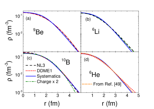
Figure 1: (Color online) Matter densities for ¹⁰B, ⁹Be, ⁶Li and ⁶He, calculated through different models (see text for details).

IV Standard Optical Model Calculations

Before providing the results of the elastic scattering data fits, we present a comparison of the experimental angular distributions with OM cross sections obtained assuming the standard models for the OP. By standard models we mean Equation (4) with $N_{R}=1$ and $N_{I}=0.78$, and Equation (5) (internal imaginary potential). From now on, we refer to these standard models as Strong Surface Absorption (SSA) and Only Internal Absorption (OIA), respectively. In order to illustrate the region of energy of the data, for each angular distribution we provide the value of the reduced energy, defined as:

$$E_{Red}=E_{c.m.}-V_{B},$$ (7)

where $E_{c.m.}$ represents the center of mass energy and $V_{B}$ is the s-wave barrier height, obtained for the respective system with the SPP. In Table III we present the barrier heights, radii and curvatures ($\hbar w$) Gasques et al. (2004), for the systems studied in the present work.

Table 3: Values of the s-wave barrier parameters obtained with the SPP for systems composed by projectiles focusing on ¹²⁰Sn.

projectile	$V_{B}$(MeV)	$R_{B}$(fm)	$\hbar w$(MeV)
4He	14.22	9.48	4.92
6He	12.78	10.52	3.35
6Li	19.76	10.16	4.20
7Li	19.45	10.34	3.86
9Be	25.78	10.40	3.93
10B	32.38	10.34	4.17
16O	50.79	10.56	4.14
18O	50.05	10.74	3.86

Figure 2 presents four experimental angular distributions for the strongly bound ⁴He projectile Mohr et al. (2010). The energies of the angular distributions vary from 5.1 to 19.1 MeV above the barrier ($5.1\leq E_{Red}\leq 19.1$ MeV). To avoid overlapping results, the cross sections for two angular distributions have been displaced by a constant factor of 0.5. The solid blue and dashed green lines represent the theoretical results obtained with SSA and OIA, respectively. Both standard models provide rather similar results, but the SSA accounts for the data with slightly better accuracy.

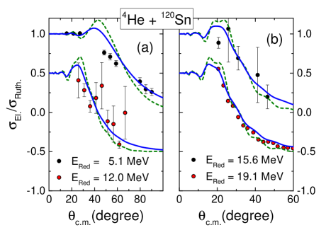
Figure 2: (Color online) Experimental angular distributions for the elastic scattering of the ⁴He + ¹²⁰Sn system Mohr et al. (2010); Kumabe et al. (1968). To avoid overlapping results, the cross sections for $E_{Red}=12.0$ and 19.1 MeV have been displaced by a constant factor of 0.5. The solid and dashed lines represent theoretical OM cross sections obtained with the SSA and OIA models, respectively.

Figure 3 presents experimental and theoretical (SSA and OIA) angular distributions for the strongly bound ¹⁶O and ¹⁸O projectiles. In the ¹⁶O case, all energies are below the corresponding barrier height. At the lowest energy ($E_{Red}=-4.0$ MeV) the data are compatible with internal absorption (OIA), while for higher energies they approach to the results of strong surface absorption (SSA). In the case of ¹⁸O, the energy is slightly above the barrier and the SSA reproduces well the data set, except at the rainbow region ($\theta_{c.m.}\approx 90^{\rm o}$).

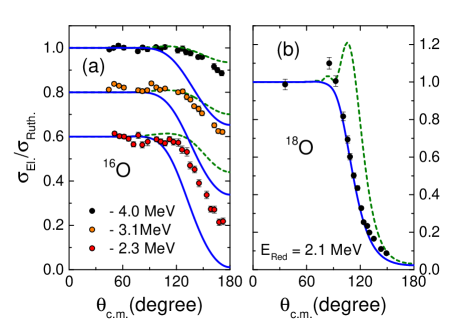
Figure 3: (Color online) Experimental angular distributions for the ^16,18O + ¹²⁰Sn systems Silva et al. (2001); Bohlen et al. (1975). To avoid overlapping results, the cross sections for some distributions have been displaced by a constant factor. The solid and dashed lines represent theoretical OM cross sections obtained with the SSA (solid) and OIA(dashed) models, respectively

Figure 4 presents data and theoretical predictions (SSA and OIA) for the elastic scattering of the exotic ⁶He on ¹²⁰Sn de Faria et al. (2010); Appannababu et al. (2019). Again the SSA provides a good description of the data, with some deviation for the lowest $E_{Red}=3.8$ and 4.4 MeV, due to transfer/break-up channels Appannababu et al. (2019).

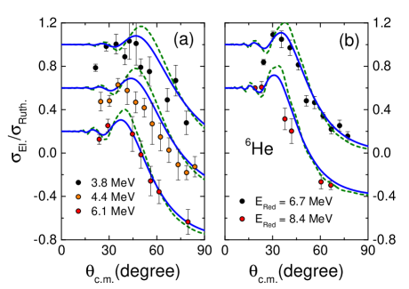
Figure 4: (Color online) The same as Fig. 3, for the ⁶He + ¹²⁰Sn system. Data were extracted from de Faria et al. (2010); Appannababu et al. (2019).

In Fig. 5, with the present new data, we show theoretical predictions for ⁶Li + ¹²⁰Sn, at energies around the barrier, in linear (a) and logarithmic (b) scales. The SSA cross sections (solid blue lines) are in good agreement with the data, including at $E_{Red}=-1.66$ MeV, which indicates strong surface absorption even in the sub-barrier energy region. For comparison, in Fig. 6 we present an excitation function for the elastic scattering of ⁶Li + ¹²⁰Sn from earlier measurements Zerva et al. (2012). The data correspond to an angular range of $160^{\rm o}\leq\theta_{Lab}\leq 170^{\rm o}$. The solid line represents the SSA cross sections at the average angle $\theta_{c.m.}=165.7^{\rm o}$. There is a reasonable agreement between experimental and theoretical results, but the slope of the data is somewhat different from that of the OM calculations.

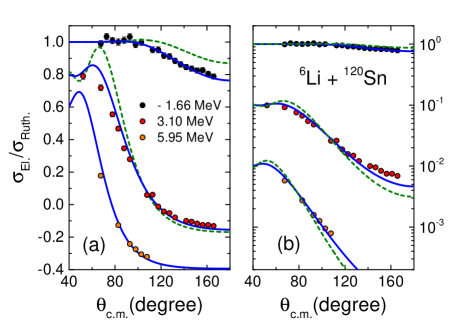
Figure 5: (Color online) Experimental and theoretical SSA (solid lines) and OIA (dashed lines) elastic scattering angular distributions for ⁶Li + ¹²⁰Sn. Note the change from linear (a) to logarithmic (b) scale. To avoid superposition, the cross sections for two distributions are displaced (a) or divided (b) by constant factors.

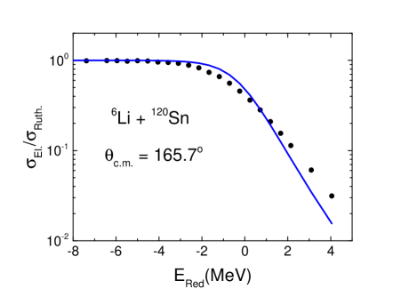
Figure 6: (Color online) Experimental excitation function for ⁶Li + ¹²⁰Sn Zerva et al. (2012) (see text for details). The solid line represents the SSA cross sections at $\theta_{c.m.}=165.7^{o}$.

Figures 7 and 8 present results for ⁷Li + ¹²⁰Sn Zagatto et al. (2017). In this case, the SSA provides even better agreement between data and theory than for ⁶Li.

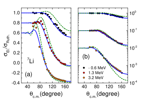
Figure 7: (Color online) The same as Fig.5, for ⁷Li + ¹²⁰Sn. Data were extracted from Zagatto et al. (2017).

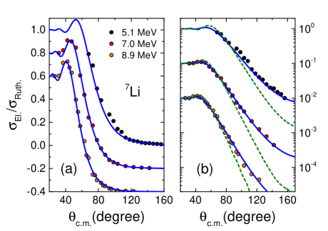
Figure 8: (Color online) The same as Fig.5, for ⁷Li + ¹²⁰Sn. Data were extracted from Zagatto et al. (2017); Kundu et al. (2017).

Figures 9 and 10 present results for ⁹Be + ¹²⁰Sn. Again, the SSA provides cross sections in reasonable agreement with the data.

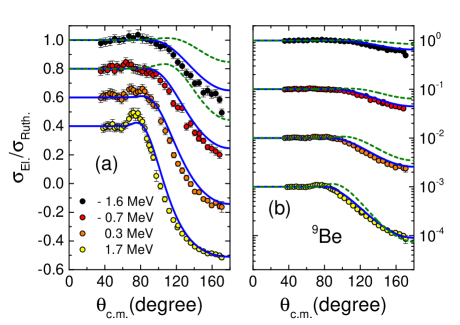
Figure 9: (Color online) The same as Fig.5, for ⁹Be + ¹²⁰Sn. Data were extracted from Arazi et al. (2018).

Figure 10: (Color online) The same as Fig.5, for ⁹Be + ¹²⁰Sn. Data were extracted from Arazi et al. (2018).

Finally, Fig. 11 presents results for ¹⁰B + ¹²⁰Sn. The SSA does not work as well as in other cases of weakly bound nuclei. However, the reduced energy region in the case of ¹⁰B is low and the results for this nucleus are similar to those shown for ¹⁶O in Fig. 3(a).

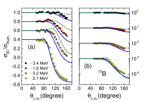
Figure 11: (Color online) The same as Fig.5, for ¹⁰B + ¹²⁰Sn. Data were extracted from Gasques et al. (2018); Alvarez et al. (2018).

V Comparison of the behavior of the optical potential for different projectiles

As commented in the previous section, the SSA provides an overall reasonable description of the complete data set studied here. Even so, small deviations between data and theoretical predictions are observed. In this section, we assume Equation (4) with two adjustable parameters, $N_{R}$ and $N_{I}$, in order to fit the data more accurately, and compare the behavior of the corresponding OP parameter values obtained for different projectiles.

V.1 The uncertainties of the $N_{R}$ and $N_{I}$ values

In this subsection, we discuss some ambiguity inherent to the extraction of the $N_{R}$ and $N_{I}$ best fit values and their respective uncertainties. For this purpose, we have performed several calculations in order to verify the sensitivity of the data fit on variations of the $N_{R}$ and $N_{I}$ parameter values. Just as an example, we illustrate here the results obtained with the data set for ¹⁸O at $E_{Red}=2.1$ MeV. The corresponding best data fit is obtained with $N_{R}=0.739$ and $N_{I}=0.877$, with reduced chi-square of $\chi^{2}=5.80$.

In Fig. 12 (a), we present the values of $\chi^{2}$ as a function of $N_{I}$ for several (fixed) values of $N_{R}$. For each $N_{R}$, there is an optimum $N_{I}$ value that provides the smallest $\chi^{2}$. Here, we can observe the strong correlation between the $N_{R}$ and $N_{I}$ parameters. This correlation can be even better observed in Fig. 12 (b), which presents the optimum $N_{I}$ value as a function of $N_{R}$. Clearly, for larger $N_{R}$ values we have smaller values of optimum $N_{I}$. In Fig. 12 (d), we show the $\chi^{2}$ (obtained with the optimum $N_{I}$) as a function of $N_{R}$. In Fig. 12 (c), we show three curves (in the $N_{R}$ - $N_{I}$ plane) that correspond to different levels of $\chi^{2}$ (and also the point that provides the best $\chi^{2}=5.80$ for this data set).

Within the context of the theory of errors, the uncertainty of an adjustable parameter can be approximately estimated considering variations of the reduced chi-square by about $1/N$ around the minimum $\chi^{2}$ value (which should be close to 1), where $N$ is the number of data. The experimental angular distribution, adopted as an example, contains 18 data points, and therefore $1/N\approx 0.06$. Since the best $\chi^{2}=5.80$, one should consider the range $\chi^{2}\leq 5.86$ for the determination of the error bars of the parameters. Nevertheless, the OM is only a simple (in fact simplified) theoretical model to describe the experimental phenomenon, and one can not expect the theory of errors to work perfectly in this case. For instance, the best $\chi^{2}=5.80$ is very far from the expected value $\chi^{2}\approx 1$ of the theory.

Taking into account this point, in many works, the estimate of uncertainties of the OM adjustable parameters is performed considering a different level of reduced chi-square, for instance, an increase of 10% or 20% relative to its minimum value. Nevertheless, oftentimes the correlation between the parameters (as that for $N_{R}$ with $N_{I}$) is not considered when determining uncertainties. In this case, the uncertainties can be largely underestimated.

Just to illustrate this point, let us suppose that we choose the level $\chi^{2}=7$ (about 20% above the best $\chi^{2}=5.80$) to determine the uncertainties. This level is represented by the dashed line in Fig. 12 (a). The solid red curve in this figure corresponds to the variation of $\chi^{2}$ as a function of $N_{I}$ for the fixed (and also the best fit value) $N_{R}=0.739$. If one neglects the $N_{R}$ - $N_{I}$ correlation, the uncertainty of the $N_{I}$ parameter is found according to the intersections of the solid red curve with the $\chi^{2}=7$ level (dashed line). The blue arrows in figure 12 (a) show the corresponding region of uncertainty: $0.86\leq N_{I}\leq 0.90$ (relative uncertainty of about 4.5%). However, an inspection of the curve corresponding to the $\chi^{2}=7$ level in Fig. 12 (c) shows that, when considering the $N_{R}$ - $N_{I}$ correlation, a better estimate for the uncertainty of $N_{I}$ is $0.76\leq N_{I}\leq 1.01$, therefore a much larger range of about 28% for the relative uncertainty. The same could be said about the $N_{R}$ uncertainty. The dashed line in Fig. 12 (d) also represents the level $\chi^{2}=7$. The corresponding $N_{R}$ region is $0.61\leq N_{R}\leq 0.84$ (about 32% of relative uncertainty in $N_{R}$). This region already contains the effect of the correlation (since the $\chi^{2}$ versus $N_{R}$ curve of Fig. 12 (b) was obtained considering the variation of the optimum $N_{I}$ value with $N_{R}$). The blue arrows that connect Figs. 12 (b) and (d) illustrate the effect of the correlation on the uncertainties of the $N_{R}$ and $N_{I}$ parameter values. In our example, the consideration or not of the correlation affects the parameter uncertainty values by a factor about 6.

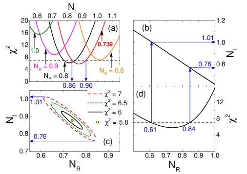
Figure 12: (Color online) The figure shows results obtained by fitting an experimental angular distribution for ¹⁸O at $E_{Red}=2.1$ MeV. (a): $\chi^{2}$ versus $N_{I}$ for some $N_{R}$ values. (b): Optimum $N_{I}$ value as a function of $N_{R}$. (c): Curves in the plane $N_{R}$ - $N_{I}$ that correspond to some levels of $\chi^{2}$. (d): $\chi^{2}$ obtained with the optimum $N_{I}$ as a function of $N_{R}$. See text for details.

Other important question can be raised here. What would be a good $\chi^{2}$ level to estimate uncertainties? In our example, we chose 20% above the best (minimum) $\chi^{2}$. The best $\chi^{2}$ is obtained with $N_{R}=0.739$ and $N_{I}=0.877$, while the borders ($\chi^{2}=7$) correspond to two possible pairs: $N_{R}=0.61$ and $N_{I}=1.01$ or $N_{R}=0.84$ and $N_{I}=0.76$. In Fig. 13 we present, in linear (a) and logarithmic (b) scales, the experimental angular distribution for ¹⁸O at $E_{Red}=2.1$ MeV, and three theoretical curves. Two of them, the solid black and dashed red lines, correspond to the best $\chi^{2}=5.80$ and to one case where $\chi^{2}=7$. These two lines are almost indistinguishable, indicating that this increase of 20% in $\chi^{2}$ is probably too small to represent actual significance. The other curve (dotted blue lines in the figure) represents the result of a fit, in which $N_{R}=1$ was fixed and only $N_{I}$ was considered as adjustable parameter. The corresponding optimum $N_{I}=0.616$ was found, with $\chi^{2}=15.54$. Despite the difference of a factor of about three between the respective $\chi^{2}$ values, both OPs (of the best $\chi^{2}=5.80$ and that with $\chi^{2}=15.54$) provide a quite reasonable data fits (see the black and blue lines in Fig. 13). The large difference between the respective $\chi^{2}$ is mostly related to the fit in the backward angular region (in particular for the datum at the last angle $\theta_{c.m.}\approx 150^{\rm o}$). On the other hand, the fit with $\chi^{2}=15.54$ (dotted blue lines in the figure) clearly provides a slightly better data description in the rainbow region ($\theta_{c.m.}\approx 90^{\rm o}$). Thus, one might ask: taking into account the physical behavior, does the fit with $\chi^{2}=5.80$ actually describe the experimental data in a better way than that with $\chi^{2}=15.54$?

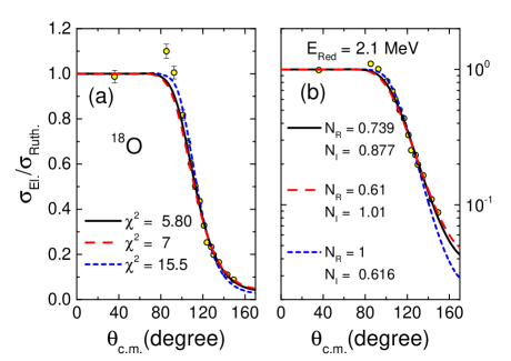
Figure 13: (Color online) Experimental angular distribution for ¹⁸O at $E_{Red}=2.1$ MeV, in linear (a) and logarithmic (b) scales. The solid black lines represent the best data fit ($\chi^{2}=5.80$) obtained within the OM. The dashed red lines were obtained with $N_{R}=0.61$ and $N_{I}=1.01$ that provide $\chi^{2}=7$. The dotted blue lines correspond to the result of the fit in which $N_{R}=1$ was fixed and only the $N_{I}$ value was adjusted ($\chi^{2}=15.54$).

Thus, uncertainties of adjustable parameter values obtained from OM data fits should be considered just as rough estimates. If the strong correlation between $N_{R}$ and $N_{I}$ is taken into account (and it should be), the uncertainties of these parameters become quite large. In addition, as commented in the previous paragraph, it is possible to obtain a quite reasonable description of the experimental angular distribution (¹⁸O at $E_{Red}=2.1$ MeV) assuming very different $N_{R}$ values. The reason for this behavior is also related to the correlation between the $N_{R}$ and $N_{I}$ parameters. As illustrated in Fig. 13, the (best fit) pair $N_{R}=0.739$ and $N_{I}=0.877$ produces OM cross sections similar to those obtained with (fixed) $N_{R}=1$ and (adjusted) $N_{I}=0.616$ (despite the large difference of a factor of 3 in the corresponding $\chi^{2}$ values).

This behavior observed for the angular distribution of ¹⁸O at $E_{Red}=2.1$ MeV is also present in many other cases (projectiles and energies). The correlation between $N_{R}$ and $N_{I}$ implies a wide ambiguity in the determination of these parameter values, when simultaneously adjusted within the context of the OM data fits. In principle, the effect of the polarization due to inelastic channels would affect both: the real and imaginary parts of the OP. Even so, in order to avoid this question of correlation and consequent ambiguity, from now on we assume $N_{R}=1$ in the OM calculations, and adjust only the $N_{I}$ parameter value in the data fits.

V.2 The sub-barrier region

When comparing data for different systems, it is important to take into account the region of energy considered. Thus, in this section we compare $N_{I}$ values obtained for different projectiles in approximately the same region of reduced energy.

As illustrated in Figs. 3 (a) and 11, at energies below the barrier, both systems, with ¹⁶O and ¹⁰B, present data with behavior in between the theoretical results of OIA (internal absorption = weak surface absorption) and SSA (strong surface absorption). In Fig. 14, we present the results obtained through OM data fits, for ¹⁶O (a) and ¹⁰B (b). The figure also shows the $N_{I}$ values obtained for each angular distribution. The ¹⁶O case presents the expected behavior of strongly bound nuclei: vanishing surface absorption at 4 MeV below the barrier ($N_{I}=0.09$), and increasing $N_{I}=0.25$ and 0.50 values when approaching the barrier. On the other hand, the $N_{I}$ values for ¹⁰B are quite similar (about 0.35) for the three energies below the barrier, indicating that the surface absorption does not decrease significantly even at sub-barrier energies.

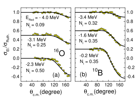
Figure 14: (Color online) Experimental angular distributions for ¹⁶O and ¹⁰B and corresponding theoretical OM cross sections obtained from data fits. The reduced energies and $N_{I}$ values are indicated in the figure.

In Fig. 15 (a), we present results for the weakly bound ⁶Li, ⁹Be and ¹⁰B projectiles, at energies about 1.6 MeV below the barrier. In pannel (b), we have ⁷Li (instead ⁶Li) and again ⁹Be and ¹⁰B, at energies about 0.5 MeV below the barrier. Even in this low energy region, the three projectiles present non vanishing $N_{I}$ values, the largest being those for ⁹Be ($N_{I}\approx 1.3$), followed by those for the lithium isotopes (about 0.7), and the small one (0.35) being that for ¹⁰B. This behavior indicates more absorption at sub-barrier energies, probably due to the break-up process, for ^6,7Li and ⁹Be Arazi et al. (2018); Luong et al. (2013).

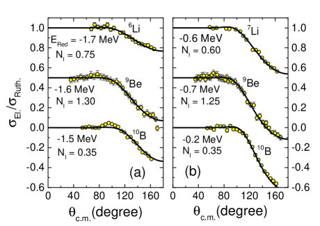
Figure 15: (Color online) The same as Fig. 14, for other systems and energies.

V.3 The above-barrier region

Now we analyze angular distributions at energies above the barrier. Again we present comparison of data only in similar reduced energy regions. For a good appreciation of the results, the figures contain both linear and logarithmic scales.

Fig. 16 presents angular distributions for ⁷Li and ⁹Be at $E_{Red}\approx 1.5$ MeV. The $N_{I}$ values of about 0.6 for ⁷Li and 1.2 for ⁹Be are quite similar to those obtained at sub-barrier energies (see Fig. 15).

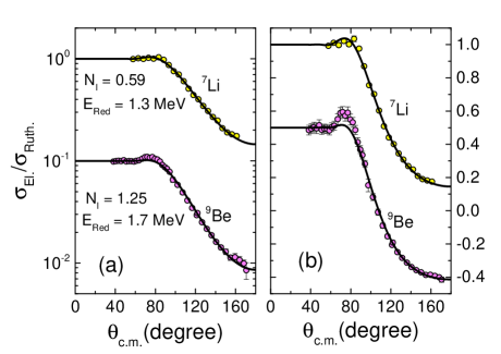
Figure 16: (Color online) Experimental angular distributions for ⁷Li and ⁹Be, in logarithmic (a) and linear (b) scales. The black lines represent the OM fits (performed by adjusting only the $N_{I}$ parameter). The corresponding $N_{I}$ and reduced energy values are indicated in the figure.

Figure 17 presents results for ⁶He, ⁶Li, ⁷Li and ⁹Be at about 3.5 MeV above the barrier. The best fit $N_{I}=4$ obtained for ⁶He is a very large value. However, we point out that, due to the large error bars of the cross section data, the sensitivity of the $\chi^{2}$ to the $N_{I}$ parameter value is very weak for this angular distribution, and much smaller $N_{I}$ values also provide a good data fit. The $N_{I}$ values obtained for the weakly bound ⁶Li, ⁷Li and ⁹Be nuclei are large, again indicating strong surface absorption in these cases.

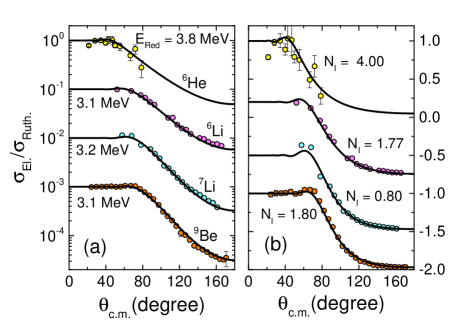
Figure 17: (Color online) The same of Fig. 16, for other projectiles and energies.

Figure 18 presents results for ⁶He, ⁶Li and ⁷Li (two energies) at $E_{Red}\approx 6$ MeV. The ⁶He and ⁶Li OM fits result in $N_{I}$ values larger than 1. The two energies for ⁷Li provide, consistently, similar values around $N_{I}\approx 0.89$.

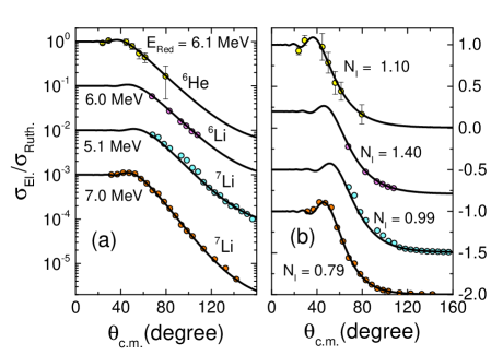
Figure 18: (Color online) The same of Fig. 16, for other projectiles and energies.

Finally, Fig. 19 presents results for the strongly bound ⁴He and the weakly bound ⁹Be nuclei, at very high energies $E_{Red}\approx 20$ MeV. A striking difference of about one order of magnitude is observed for the corresponding $N_{I}$ values: 0.20 and 1.90.

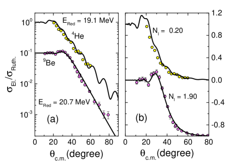
Figure 19: (Color online) The same of Fig. 16, for other projectiles and energies.

In Fig. 20, we show the $N_{I}$ values as a function of the reduced energy for several projectiles. We have not included the results for ⁶He and ⁴He, at low energies, because the $\chi^{2}$ for these distributions are not very sensitive to the $N_{I}$ values, due to the large error bars of the experimental cross sections. The solid lines in this figure are only guides for the eyes. The dashed line corresponds to the standard $N_{I}=0.78$ value. Considering only the behavior of the weakly bound nuclei, the figure indicates increasing $N_{I}$ parameter values in the following order: ¹⁰B, ⁷Li, ⁶Li and ⁹Be.

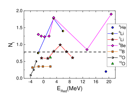
Figure 20: (Color online) $N_{I}$ values obtained from OM data analyses as a function of the reduced energy for several projectiles. The solid lines in the figure are only guides for the eyes, while the dashed line corresponds to the standard $N_{I}=0.78$.

VI Conclusions

In this paper, we have presented new data for the elastic scattering of ⁶Li + ¹²⁰Sn at $E_{\rm LAB}=$ 19, 24 and 27 MeV. The corresponding angular distributions were considered together with other elastic scattering data of several projectiles on the same target nucleus. The complete data set was systematically analyzed within the context of the OM. We have demonstrated that the SPP in the context of the standard SSA provides a quite reasonable description of the data for all systems, without the necessity of any adjustable parameter. We have obtained more accurate agreement between data and theoretical cross sections by considering adjustable OP strengths in order to improve the data fits.

We have illustrated the strong correlation between the real and imaginary adjustable strength factors ($N_{R}$ and $N_{I}$) in an example with one angular distribution. If this correlation is taken into account, the uncertainties of the $N_{R}$ and $N_{I}$ best fit values become very large. In addition, different pairs of these parameters, with corresponding $\chi^{2}$ values that differ by a factor as large as 3, provide rather similar theoretical angular distributions that agree well with the data. This behavior is also found for other projectiles and energies. In order to avoid this ambiguity, we have assumed the SPP for the real part of the OP, with fixed standard $N_{R}=1$, and adjusted only the $N_{I}$ parameter value in the OM data fits.

As observed in Figs. 14 to 19, the theoretical cross sections obtained through OM fits with only one free parameter ($N_{I}$) are in quite good agreement with the data for all systems and energies. We have studied the behavior of the best fit $N_{I}$ value in different energy regions, and compared results obtained for the various projectiles. The weakly bound ^6,7Li, ⁹Be and ¹⁰B projectiles present significant $N_{I}$ values at sub-barrier energies, indicating strong surface absorption even in this low energy region, a characteristic probably related to the break-up process. Still considering these nuclei, increasing $N_{I}$ parameter values are observed in the following order: ¹⁰B, ⁷Li, ⁶Li and ⁹Be. This order is related to the binding energy of these nuclei (presented as $Q$ values in Table I). This suggests a clear correlation between the break-up probability and the absorption of flux from the elastic channel.