Abstract

Sperm of marine invertebrates have to find eggs cells in the ocean. Turbulent flows mix sperm and egg cells up to the millimeter scale; below this, active swimming and chemotaxis become important. Previous work addressed either turbulent mixing or chemotaxis in still water. Here, we present a general theory of sperm chemotaxis inside the smallest eddies of turbulent flow, where signaling molecules released by egg cells are spread into thin concentration filaments. Sperm cells ‘surf’ along these filaments towards the egg. External flows make filaments longer, but also thinner. These opposing effects set an optimal flow strength. The optimum predicted by our theory matches flow measurements in shallow coastal waters. Our theory quantitatively agrees with two previous fertilization experiments in Taylor-Couette chambers and provides a mechanistic understanding of these early experiments. ‘Surfing along concentration filaments’ could be a paradigm for navigation in complex environments in the presence of turbulent flow.

Introduction

Chemotaxis - the navigation of biological cells guided by chemical gradients - is crucial for bacterial foraging, neuronal development, immune responses, and sperm-egg encounter during fertilization [1, 2, 3, 4, 5]. Despite a century of research, most studies assumed perfect concentration gradients of signaling molecules. Yet, in natural environments, concentration fields of these chemoattractants are non-ideal, distorted e.g. by turbulent flows. An unusually accessible model system of such a cellular navigation is the chemotaxis of sperm cells in marine invertebrates with external fertilization. For fertilization, sperm cells of many species are known to employ chemotaxis to steer up concentration gradients of signaling molecules released by the egg. This sperm chemotaxis has been intensively studied for external fertilization of marine invertebrates, where sperm and egg cells are spawned directly into the sea [6, 5, 7, 8, 9]. In this case, sperm and egg cells become strongly diluted. Besides synchronized spawning [10, 11], sperm chemotaxis is important to enhance sperm-egg encounter rates [12]. The mechanism of sperm chemotaxis in marine invertebrates is well established theoretically [13, 14] and has been experimentally confirmed [15]: Sperm cells swim along helical paths $\mathbf{r}(t)$, while probing the surrounding concentration field $c(\mathbf{r})$. A cellular signaling system rotates the helix axis $\mathbf{h}$ to align with the gradient $\bm{\nabla}c$ at a rate proportional to a normalized gradient gradient strength $\left|\bm{\nabla}c\right|/\left(c+c_{b}\right)$ reflecting sensory adaption with sensitivity threshold $c_{b}$ [16, 17].

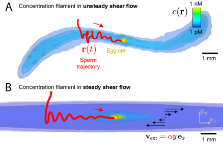
Figure 1: Sperm chemotaxis in external flow. (A) Simulated, three-dimensional concentration field $c(\mathbf{r})$ of chemoattractant released from a freely-rotating, spherical egg (yellow sphere) suspended in unsteady shear flow as a model of small-scale turbulence. An exemplary simulated sperm cell (trajectory in red) finds the elongated concentration filament by chance and subsequently ‘surfs’ along the filament by chemotaxis (B) Same as (A), but for the prototypical idealization of simple shear flow $\mathbf{v}_{\text{ext}}(\mathbf{r})=\alpha y\,\mathbf{e}_{x}$ accounting for convection and co-rotation by the external flow. We obtain a generic form of the concentration filament, Eq. (1), and characterize surfing along the filament analytically as a damped oscillation. Parameters correspond to sea urchin A. punctuala, assuming continuous release of chemoattractant at constant rate $\dot{Q}=0.46\leavevmode\nobreak\ \text{fmol min}^{-1}$ for an exposure time $t_{\text{max}}=6\leavevmode\nobreak\ \text{min}$. Constant shear rate $\alpha=0.17\leavevmode\nobreak\ \text{s}^{-1}$ in (B), corresponding to root-mean-square shear rate of (A). Same color-code for concentration in (A) and (B), but different level sets. We use a generic theoretical description of helical sperm chemotaxis, see Methods and Materials for details (helix radius $r_{0}=7\leavevmode\nobreak\ \mu\text{m}$ not visible at length-scale of figure).

Previous work on sperm chemotaxis focused predominantly on idealized conditions of still water [18, 9]. However, natural habitats like the ocean are characterized by turbulent flow, which convects and co-rotates gametes and distorts concentration fields into filamentous plumes [7, 19, 20, 21, 16, 22, 23], see Fig 1A for illustration. Turbulence in typical spawning habitats of marine invertebrates has been characterized, e.g., in terms of local energy dissipation rates per mass $\epsilon=10^{-9}-10^{-6}\leavevmode\nobreak\ \text{m}^{2}\text{s}^{-3}$ [24, 25, 19, 26, 22] corresponding to typical shear rates $\alpha=0.03-1\leavevmode\nobreak\ \text{s}^{-1}$, which are often similar to those in mammalian reproductive tracts [5]. Turbulent flow rapidly mixes sperm and egg cells, yet only down to the Kolmogorov length-scale $\eta_{\text{Kol}}=\left(\nu^{3}/\epsilon\right)^{1/4}=1-10\leavevmode\nobreak\ \text{mm}$ (with kinematic viscosity $\nu$). Previous predictions based on turbulent mixing [27] substantially underestimated fertilization probability $P_{\text{fert}}$ [28, 22], since these early studies neglected active swimming and sperm chemotaxis inside the smallest eddies, whose size is comparable to the Kolmogorov length $\eta_{\text{Kol}}$. At these small length-scales, the Reynolds number of the flow is below one, and gametes perceive turbulence as unsteady shear flow [24, 26] with a typical shear rate $\alpha$ set by the inverse of the Kolmogorov time $\tau_{\text{Kol}}=\sqrt{\nu/\epsilon}$. Intriguingly, fertilization experiments conducted at physiological shear rates hint at the existence of an optimal shear rate $\alpha^{*}>0$, corresponding to an optimal turbulence strength $\epsilon^{*}>0$, at which the fertilization probability $P_{\text{fert}}$ was maximal [25, 20, 29]. Similar observations have been made in direct numerical simulations of bacterial chemotaxis [21]. Obvious biological effects can be ruled out as the origin of the optimum [25, 19], including flow damaging the gametes or sperm-egg bonds being broken by shear forces. Despite an early two-dimensional model [29], a physical explanation and quantitative understanding of the observed optimum is still missing [20, 22].

Here, we develop a theory of sperm chemotaxis in small-scale turbulence: As a prototypical model, we consider sperm chemotaxis in simple, three-dimensional shear flow, which convects and co-rotates sperm cells and distorts the chemoattractant field that surrounds the egg. We predict an optimal shear rate $\alpha^{*}$ in simulations, as previously suggested by experiments [25, 20]. We provide a novel mechanistic explanation of this optimum from theory: We describe how external flow distorts concentration fields into slender filaments, and how sperm cells ‘surf’ along these filaments towards the concentration source, see Fig 1B. The optimum arises from the competition between accelerated spreading of the chemoattractant at increased flow, which enhances chemotaxis, and filaments becoming increasingly thinner, which impairs chemotaxis. We apply our theoretical description to two previous experiments on sperm chemotaxis, one with moderate flow, mimicking fertilization in shallow coastal waters [20], and one with strong turbulence, mimicking fertilization in the surf zone [25]. In both cases, simulation and theory match the experimental data, yet also prompt a partial re-interpretation of these early experiments: We infer a high background concentration of chemoattractant in these experiments, which actually masks the existence of an optimal flow strength for the experimental conditions used (in contrast to physiological spawning habitats where no relevant background concentration should be present). We propose that ‘surfing along concentration filaments’ could be a common navigation paradigm in natural habitats characterized by external flows, which is relevant for the last millimeters towards a source.

Results

Simulations: Optimal shear rate

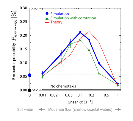
Figure 2: Sperm-egg-encounter probability displays maximum as function of shear rate in simulations for sea urchin sperm at physiological flow rates. Probability $P_{\text{sperm:egg}}(\alpha)$ that a single sperm cell finds an egg as function of external shear rate $\alpha$. Simulations account for flow-induced distortion of concentration fields into long filaments as well as convection and co-rotation of sperm cells by the flow (green triangles, mean $\pm$ SD). Without co-rotation results change only marginally (blue circles). Simulation results agree with predictions from our theory of filament surfing (red, presented below). Without sperm chemotaxis, the encounter probability is virtually zero ($<10^{-5}$, black). Our theory has a single fit parameter, the flux of sperm cells arriving at the filament, $j_{\text{out}}=0.063\leavevmode\nobreak\ \text{m}^{-2}\text{s}^{-1}$. This value matches in magnitude the limit $j_{\text{out}}=\rho_{\text{egg}}v_{h}/4=0.04\leavevmode\nobreak\ \text{m}^{-2}\text{s}^{-1}$ for a ballistic swimmer with random initial conditions, see Sec. E for details. Parameters as in Fig 1B.

We simulate sperm chemotaxis in a simple shear flow $\mathbf{v}_{\text{ext}}\left(\mathbf{r}\right)=\alpha y\,\mathbf{e}_{x}$, extending a generic theory of helical chemotaxis [14] by incorporating convection and co-rotation of sperm cells by the external fluid flow. In particular, for co-rotation by the flow the Jeffery equation [30, 31] is employed. We ask for encounters of sperm cells with a single egg that releases chemoattractant molecules, which establish a concentration field $c(\mathbf{x},t)$ by convection and diffusion. By switching to a co-moving frame in which the egg is at rest. we may assume that the suspended egg is located at the origin $\mathbf{r}=\mathbf{0}$ without loss of generality. We use a spherical periodic boundary at radius $r_{\text{max}}$, which mimics an ensemble of eggs with density $\rho_{\text{egg}}=\left(4\pi r_{\text{max}}^{3}/3\right)^{-1}$, and assume an exposure time $t_{\text{max}}$. For turbulent flow, the exposure time would correspond to a typical time interval between subsequent intermittency events that re-mix sperm and egg cells and reset any concentration field of chemoattractant that might have been established in between. (Methods and Materials provides details on simulation setup and extensive discussion of parameters.) The resulting sperm-egg-encounter probability $P_{\text{sperm:egg}}$ displays a maximum at an optimal shear rate $\alpha^{*}\approx 0.1\leavevmode\nobreak\ \text{s}^{-1}$, see Fig 2, which uses parameters for sea urchin A. punctuala. At the optimal shear rate $\alpha^{*}$, $P_{\text{sperm:egg}}$ is $4$-fold higher than without flow. Only for larger shear rates $\alpha>0.3\leavevmode\nobreak\ \text{s}^{-1}$, chemotaxis becomes less effective than without flow and finally ineffective at very strong shear rate with $\alpha\geq 1\leavevmode\nobreak\ \text{s}^{-1}$. Note that without chemotaxis, the encounter probability is 2-3 orders of magnitude smaller for the chosen parameters (not shown as not visible).

Surprisingly, the numerical results show that co-rotation of sperm cells is not necessary for the existence of an optimal shear rate as simulations without co-rotation yield very similar results, see Fig 2. Consequently, the existence of an optimal shear rate $\alpha^{*}$ should be a consequence of the distortion of the concentration field by the flow. For simplicity, we thus focus on the case without co-rotation in the following (simulations with co-rotation are displayed in Figs A and C ). Typically, shear flow generates long filaments, or plumes, of high concentration. Simulations show how sperm cells enter these filaments and ‘surf’ along them, see Fig 1B, with trajectories resembling a damped oscillation, see also Fig D. Damped oscillations occur when sperm cells move towards the egg, yet oscillations are amplified when sperm cells move away from the egg. The latter sometimes causes sperm cells swimming in the wrong direction to turn around, thus redirecting them towards the egg. In conclusion, sperm chemotaxis in external flows is a two-stage search problem [32] of first finding a concentration filament and subsequent chemotactic surfing along this filament towards the egg.

Theory: Filament surfing

We develop a theory of sperm chemotaxis in filamentous concentration fields generated by simple shear flows. This theory describes surfing along filaments and allows to predict the sperm-egg-encounter probability, see Fig 2. We consider a simple shear flow $\mathbf{v}_{\text{ext}}\left(\mathbf{r}\right)=\alpha y\,\mathbf{e}_{x}$ and a spherical egg of radius $r_{\text{egg}}$, without loss of generality located at $\mathbf{r}=\mathbf{0}$, releasing chemoattractant at a constant rate for a time $t$. The choice of the coordinate system corresponds to a co-moving frame in which the egg is at rest. Far from the source $\left|\mathbf{r}\right|\gg r_{\text{egg}}$, the concentration field $c(\mathbf{r},t)$ established by diffusion and convection takes a generic form, see Fig 1B for illustration,

$$c(\mathbf{r},t)=c_{0}\exp\left(-k\left|x\right|\right)\exp\left(-\frac{\left(y-y_{0}\right)^{2}/a_{y}^{2}+z^{2}}{2\sigma^{2}}\right)\ .$$ (1)

Eq. (1) describes a filament with exponential decay along its center line $\left(x,y_{0}(x,t),0\right)$ and a Gaussian cross-sectional profile. We derived phenomenological power-laws for all parameters $c_{0}(t)$, $k(t)$, $\sigma(\left|x\right|,t)$, $a_{y}$, and $y_{0}(x,t)$, see Sec. C for details. Importantly, the effective decay length along the centerline of the concentration filaments increases with flow, $1/k\sim\alpha$, while the effective diameter of the filaments decreases with flow, since the decay length $\sigma$ away from the centerline of the filaments is independent of the flow while the base concentration $c_{0}$ decreases with flow, $c_{0}\sim\alpha^{-1}$. In this sense, the concentration filaments become longer and thinner with increasing shear rate $\alpha$.

Sperm cells from marine invertebrates swim along helical paths, along which they measure the local concentration of chemoattractant [15]. This time-dependent concentration signal exhibits characteristic oscillations at the frequency of helical swimming, which encode direction and strength of a local concentration gradient. The concentration signal elicits a continuous steering response by which the helical swimming path aligns with the gradient. We generalize an effective equation for the alignment of the helix axis $\mathbf{h}(t)$ with the local gradient $\bm{\nabla}c(\mathbf{r}(t))$, previously derived for simple radial concentration fields [14],

$$\dot{\Psi} =-v_{\varphi}\frac{\left|\bm{\nabla}c\right|}{c+c_{b}}\sin\Psi\ ,\qquad\Psi=\sphericalangle\left(\bm{\nabla}c,\mathbf{h}\right)\ ,$$ (2)

with an effective response parameter $v_{\varphi}$ of chemotactic signaling, to concentration filaments given by Eq. (1), see Sec. D for details. For a normalized distance $Y$ of the sperm trajectory from the centerline of the concentration filament, we obtain a one-dimensional effective equation of motion which explains and quantifies filament surfing,

$$\ddot{Y}=\big{(}\underbrace{-\left(1-\dot{Y}^{2}\right)Y}_{\sim\text{oscillator}}\pm\underbrace{\gamma\sqrt{\left(1-\dot{Y}^{2}\right)}\dot{Y}}_{\sim\text{damping}}\big{)}\underbrace{\frac{c}{c+c_{b}}}_{\sim\text{dimmer switch}}\ .$$ (3)

The single dimensionless parameter $\gamma$ depends on the geometry of the concentration filament and chemotaxis parameters: $\gamma$ decreases for longer and thinner filaments, while it increases with a rate of chemotactic re-orientation, see Sec. D for details. To leading order, the effective equation of motion Eq. (3) represents a damped harmonic oscillator. The corresponding frequency and damping ratio match the damped oscillation observed in simulations, see Fig 1 and Fig D. The strong gradient in the cross-section of the filament causes sperm cells to navigate towards the centerline of the filament. Yet, cells continuously pass through this centerline due to their finite chemotactic turning rate and consequently oscillate within the filament. The much weaker gradient along the concentration filament in Eq. (1) damps this oscillation when sperm cells move towards the egg, and amplifies it when they move away.

The threshold $c_{b}$ of sensory adaption limits chemotaxis to the part of the filament with concentration at least of the order of $c_{b}$. This defines a cross-sectional area $A(x)$, where $c(\mathbf{r})\geq c_{b}$, as well as circumference $S(x)$, at each centerline position $x$ of the filament. We decompose the search for the egg into an outer search, i.e., finding the concentration filament, and an inner search, i.e., surfing along the filament, see Sec. E. For the outer search, we introduce the flux $j_{\text{out}}$ of sperm cells arriving at the surface of the concentration filament and assume that $j_{\text{out}}$ is approximately independent of the position $x$ along the filament. Given that the egg has to be found within the exposure time $t_{\text{max}}$, we also introduce the outer search time $t_{\text{out}}(x,t_{\text{max}})<t_{\text{max}}$ available to arrive at the filament at $x$ as specified below. For the inner search, using the effective equation of motion, we compute the probability $p_{\text{in}}(x,t_{\text{max}})$ that a sperm cell entering the filament at position $x$ reaches the egg within time $t_{\text{max}}$. We also compute the conditional mean surfing time $t_{\text{in}}(x,t_{\text{max}})$, i.e., the average time successful sperm cells require to reach the egg after entering the filament at $x$. Correspondingly, we set the time for the outer search as $t_{\text{out}}(x,t_{\text{max}})=t_{\text{max}}-t_{\text{in}}(x,t_{\text{max}})$ for $p_{\text{in}}>0$ (and $t_{\text{out}}=0$ for $p_{\text{in}}=0$). With these prerequisites, we can formulate a general formula for the sperm-egg encounter probability $P_{\text{sperm:egg}}$ in the presence of shear flow

$$P_{\text{sperm:egg}}\approx\int\limits_{-r_{\text{max}}}^{r_{\text{max}}}\mathrm{d}x\,p_{\text{in}}(x,t_{\text{max}})\Big{[}A(x)\rho_{\text{egg}}+S(x)j_{\text{out}}t_{\text{out}}(x,t_{\text{max}})\Big{]}\ .$$ (4)

The first term approximates the contribution from sperm cells that are initially within the filament. This contribution is negligible compared to the second term for low $\rho_{\text{egg}}$ or large $t_{\text{max}}$. The second term quantifies the contribution from sperm cells that successfully find the concentration filament and surf along it to the egg. The flux $j_{\text{out}}$ can be determined either from a fit to full simulations or approximated as $j_{\text{out}}=\rho_{\text{egg}}v_{h}/4$ by treating sperm cells outside the filament as ballistic swimmers with speed $v_{h}$, see Sec. E, both of which gives similar results. Moreover, the approximation of a ballistic swimming path outside of the filament is reasonable, as the persistence length of sperm swimming paths in the absence of chemoattractant cues was estimated as $3-25\leavevmode\nobreak\ \text{mm}$ [33], which is much greater than the diameter of concentration filaments.

Note that for the chosen parameters, the volume $V_{\text{tot}}=\int_{-\infty}^{\infty}\mathrm{d}x\,A(x)$ of the filament (and its surface area $\int_{-\infty}^{\infty}\mathrm{d}x\,S(x)$) increases monotonically with shear rate $\alpha$. Hence, the optimal $\alpha^{*}$ is not explained by a flow-dependent ‘chemotactic volume’ $V_{\text{tot}}$. Instead, the optimum emerges from two effects related to filament surfing, which reduce $p_{\text{in}}$ and $t_{\text{out}}$ in Eq. (4) at high $\alpha$: First, when the filament is too thin at the entry point $x$ to enable the first oscillation, the sperm cells simply pass through the filament, which corresponds to low or vanishing probability $p_{\text{in}}$. Second, if the time required to surf from the entry point $x$ to the egg is too long, which corresponds to low or vanishing $t_{\text{out}}$, the sperm cells will not reach the egg during the exposure time $t_{\text{max}}$. Higher shear rates generate longer and thinner filaments, which aggravates both effects.

Comparison of full simulations and the theoretical prediction Eq. (4) shows good agreement, see Fig 2. This agreement strongly suggests that the optimal shear rate $\alpha^{*}$ originates from two competing effects: Higher shear flow spreads the chemoattractant faster, which facilitates sperm navigation to the egg, but results in longer and thinner filaments, which impairs chemotactic filament surfing. The value of the optimal shear rate $\alpha^{*}$ could be adjusted to a different value by re-scaling the biological parameters that involve a time-scale such as the diffusion coefficient and release rate of chemoattractant or the swimming and chemotactic re-orientation speed of sperm cells, see Sec. D .

According to our theory, the presence of an optimal flow strength is a generic feature at low egg densities and relatively long exposure times. Amplitude and position of the peak of the sperm-egg-encounter probability $P_{\text{sperm:egg}}(\alpha^{*})$ depend on chosen parameters. Our theory allows to compute $P_{\text{sperm:egg}}(\alpha)$ for any given set of parameters and thus the parameter-dependency of the optimal shear rate $\alpha^{*}$ can be explored. A numerical parameter study is presented in Sec. I, which demonstrates the robustness of the existence of an optimal shear rate under parameter variation. In short, a higher egg density $\rho_{\text{egg}}$ and longer exposure time $t_{\text{max}}$ increase the absolute amplitude $P_{\text{fert}}(\alpha^{*})$ of this peak, while $\alpha^{*}$ stays almost constant. A high sensitivity threshold $c_{b}$ of chemotactic signaling, which is formally analogous to a high background concentration of chemoattractant, reduces the relative amplitude $P_{\text{sperm:egg}}(\alpha^{*})/P_{\text{sperm:egg}}(\alpha=0)$ of the peak. Significantly shorter exposure time $t_{\text{max}}$ or higher egg density $\rho_{\text{egg}}$ reduce $p_{\text{in}}$ by effectively cutting off the outer parts of the filament. Note that the optimal shear rate $\alpha^{*}$ is slightly smaller in simulations, compared to the theory. Inspection of simulated trajectories suggest that this is due to sperm cells, which miss the egg at least once while surfing along the filament, which increases the mean surfing time $t_{\text{in}}$.

Comparison with experiments

Previous experiments measured the fraction of fertilized eggs $P_{\text{fert}}$ for an exposure time $t_{\text{max}}$. This fraction directly relates to the encounter probability $P_{\text{sperm:egg}}$ by fertilization kinetics [34, 35] when the respective densities of sperm and egg cells, $\rho_{\text{sperm}}$ and $\rho_{\text{egg}}$, are known

$$P_{\text{fert}}(t_{\text{max}})=1-\exp\left(-p_{\text{f}}P_{\text{sperm:egg}}(t_{\text{max}})\frac{\rho_{\text{sperm}}}{\rho_{\text{egg}}}\right)\ .$$ (5)

The fertilizability $p_{\text{f}}$ is the probability that a sperm-egg-encounter results in successful fertilization. Note that a local maximum of the encounter probability $P_{\text{sperm:egg}}$ at some optimal shear rate $\alpha^{*}$ automatically gives a local maximum of the fertilization probability $P_{\text{fert}}$. In particular, the density of sperm only alters the absolute value of $P_{\text{fert}}$ across all shear rates but not the existence and value of an optimal shear rate $\alpha^{*}$.

Moderate shear

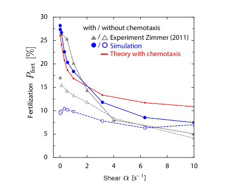
Figure 3: Comparison to experiment at moderate shear rates and short exposure time. Fertilization probability $P_{\text{fert}}(\alpha)$ that an egg becomes fertilized as function of external shear rate $\alpha$ from previous experiments with red abalone H. rufescens gametes in a Taylor-Couette chamber (filled gray triangles: with chemotaxis, open gray triangles: inhibited chemotaxis; for $\alpha=0\leavevmode\nobreak\ \text{s}^{-1}$ a different experimental protocol was used) [20] and our corresponding simulations (filled blue circles: with chemotaxis, open blue circles: without chemotaxis, mean $\pm$ SD). We find reasonable agreement using a single fit parameter, fertilizability $p_{\text{f}}\approx 60\%$, which characterizes the fraction of sperm-egg encounters that result in successful fertilization, see Eq. (5). From the experimental protocol, we estimate a background concentration $c_{\text{bg}}\sim 4\leavevmode\nobreak\ \text{nM}$ of chemoattractant. While our theory of filament surfing does not directly apply due to this high background concentration, a near-field estimate (red line) yields a similar decay of fertilization probability as function of shear rate $\alpha$. The single fit parameter of the theory, $j_{\text{out}}=4.8\cdot 10^{3}\leavevmode\nobreak\ \text{m}^{-2}\text{s}^{-1}$, is again consistent with the limit $j_{\text{out}}=\rho_{\text{egg}}v_{h}/4=7.5\cdot 10^{3}\leavevmode\nobreak\ \text{m}^{-2}\text{s}^{-1}$ of a ballistic swimmer with random initial conditions (note the the higher value of $j_{\text{out}}$ compared to Fig 2 due to higher egg density). For simplicity, simulations do not account for co-rotation of sperm cells, see Fig A for results with co-rotation.

In a previous experiment by Zimmer and Riffell, fertilization was studied for red abalone H. rufescens in a Taylor-Couette chamber for moderate shear rate $\alpha$, mimicking flow conditions in their natural spawning habitat [19, 20]. The measured fertilization probability decreased with increasing $\alpha>0$, both for normal chemotaxis and a case of chemically inhibited chemotaxis, see Fig 3 for a reproduction of the original data ([20], Fig. 5c). At low shear rate, the measured fertilization probability is twice as high with chemotaxis than without, while there was little difference at high shear rates. This suggests that the performance of sperm chemotaxis is reduced at high shear rates. We performed simulations of sperm chemotaxis in external flow, using parameters that match the specific experimental setup of [19, 20], see Sec. G. Specifically, the time span between preparation of the egg suspension and the actual fertilization experiment results in a background concentration of chemotattractant, which we estimate as $c_{\text{bg}}\sim 4\leavevmode\nobreak\ \text{nM}$, i.e., several orders of magnitude larger than the threshold of sensory adaption $c_{b}$, and account for in the simulations. We compare results of these simulations and the experiments, using fertilizability $p_{\text{f}}$ as single fit parameter, see Fig 3. We find good agreement for the case with normal chemotaxis, and reasonable agreement for the case of inhibited chemotaxis (potentially due to residual chemotaxis in the latter case). An exception is the data point at $\alpha=0\leavevmode\nobreak\ \text{s}^{-1}$. In fact, a different experimental protocol was used for this data point, corresponding to different initial mixing of sperm and egg cells, which is not modeled in the simulations. In Fig 3, we neglected co-rotation of sperm cells for simplicity. We find similar results if we account for co-rotation, except for the highest shear rates, where fertilization probability is reduced, see Fig A. For simplicity, a shear rate dependent chemokinesis as suggested by [19, 20], i.e., regulation of sperm swimming speed, is not included in the model, as preliminary simulations suggest that this changes results only slightly. In our comparison, we focused on the case of low sperm density considered in [19, 20], thereby avoiding confounding effects of sperm-sperm interactions and reduced fertilization rates due to polyspermy at high sperm densities [36, 37].

The absence of an optimal shear rate $\alpha^{*}$ is caused by the high background concentration $c_{\text{bg}}$ in the experiment: Due to $c_{\text{bg}}$, the part of the filament with sufficiently high concentration $c(\mathbf{r})\gtrsim c_{b}+c_{\text{bg}}$ is situated only in the vicinity of the egg and has an approximately spherical shape. While our far-field theory of filament surfing does not directly apply to this special near-field case, a simple estimate for $p_{\text{in}}$ and $t_{\text{out}}$ assuming straight sperm trajectories aligned with the local concentration gradient inside the plume, see Sec. E, yields a similar decay of fertilization probability, see Fig 3. The fitted flux of sperm cells into the concentration plume $j_{\text{out}}=4.8\cdot 10^{3}\leavevmode\nobreak\ \text{m}^{-2}\text{s}^{-1}$ is consistent with the limit $j_{\text{out}}=\rho_{\text{egg}}v_{h}/4=7.5\cdot 10^{3}\leavevmode\nobreak\ \text{m}^{-2}\text{s}^{-1}$ for a ballistic swimmer. This validates our interpretation of chemotaxis in external shear as a two-stage search, consisting of blind random search for a chemotactic volume and subsequent navigation inside this volume. We emphasize that the high background concentration of chemoattractant, which we reconstruct for these experiments, has a strong effect on the fertilization dynamics. Such high background concentrations are unlikely to be encountered in natural habitats, where eggs are spawned and consequently diluted in the open water.

Strong flows

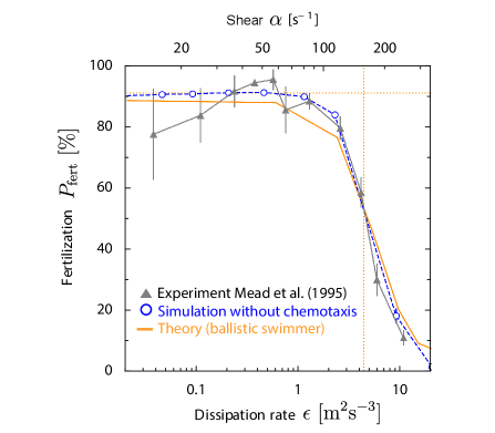
Figure 4: Fertilization in strong flows and high egg density. Previous measurements of fertilization probability $P_{\text{fert}}(\epsilon)$ for sea urchin S. purpuratus at strong turbulence, characterized by density-normalized dissipation rate $\epsilon$ (filled gray triangles) [25, 38] and our corresponding simulations $P_{\text{fert}}(\alpha)$ as function of shear rate $\alpha$ (open blue circles, mean $\pm$ SD) match well, using a single fit parameter $a=0.075$ that relates dissipation rate $\epsilon$ and typical shear rate $\alpha$ (using the known relationship $\alpha(\epsilon)=a\sqrt{\epsilon/\nu}$ [24, 26]). Both simulation and experiment are well captured by a minimal theory of a ballistic swimmer in simple shear flow (red), see Sec. A. Fertilization probability $P_{\text{fert}}$ rapidly drops above a characteristic flow strength $\alpha>100\leavevmode\nobreak\ \text{s}^{-1}$, which is consistent with a scale estimate $\alpha=2\pi v_{h}/(0.1r_{\text{egg}})$ (vertical dotted line). At these high shear rates, active swimming becomes negligible compared to convection. The case of low shear rates is well described by the limit case of a ballistic swimmer in the absence of flow $\alpha=0\leavevmode\nobreak\ \text{s}^{-1}$ (dotted horizontal line, Eq. (5) with $P_{\text{sperm:egg}}(t)=1-\exp(-qt)$ and rate $q=\pi r_{\text{egg}}^{2}v_{h}\rho_{\text{egg}}$). The fertilizability $p_{\text{f}}=10\%$ is obtained from an independent experiment [25], see Fig B. From the experimental protocol, we estimate a high background concentration $c_{\text{bg}}=500-4000\leavevmode\nobreak\ \text{nM}$ of chemoattractant, which renders sperm chemotaxis ineffective. Corresponding results for simulations with co-rotation are shown in Fig C.

Mead and Denny studied fertilization in the sea urchin S. purpuratus in turbulent flow, mimicking physiological conditions in the oceanic surf zone [25, 39, 38]. The measured fertilization probability slightly increased as function of turbulence strength, quantified in terms of local dissipation rate $\epsilon$, and decreased rapidly at larger dissipation rate $\epsilon>1\leavevmode\nobreak\ \text{m}^{2}\text{s}^{-3}$, see Fig 4 for a reproduction of the original data (taken from Fig. 3 of [38], representing a re-calibration of data from Fig. 5 of [25]). We determined fertilization probability $P_{\text{fert}}$ in simple shear flow from simulations, using parameters that match the specific experimental setup, see Sec. G. For the experiments by Mead and Denny, we estimate a high background concentration of chemoattractant $c_{\text{bg}}=500-4000\leavevmode\nobreak\ \text{nM}$, which renders sperm chemotaxis ineffective, which is thus neglected in the simulations. Fully developed turbulence is characterized by a spectrum of local shear rates, with a characteristic shear rate $\alpha$ related to the dissipation rate by $\alpha(\epsilon)=a\sqrt{\epsilon/\nu}$ with proportionality factor $a$ [24, 26]. In the simulations, we assume a simple shear flow $\mathbf{v}_{\text{ext}}=\alpha y\,\mathbf{e}_{x}$, and determine $a=0.075$ by a single-parameter fit, see Fig 4. For sake of simplicity, co-rotation of sperm cells is neglected. Results with co-rotation are qualitatively very similar, yet the fertilization probability $P_{\text{fert}}$ drops at a smaller shear rate $\alpha$ and thus yields a smaller fit parameter $a=0.023$, see Fig C. Note that these fits for $a$ are smaller than values commonly used in the literature $a\sim 0.15-1.8$ [40, 41, 24]. Nevertheless, our minimal model already reproduces the experimentally observed characteristic drop in fertilization probability $P_{\text{fert}}(\epsilon)$ at high flow rates, implying that this is a robust, general feature.

We can capture the functional dependence of the fertilization probability $P_{\text{fert}}$ observed in both experiment and simulations by a minimal theory of a ballistic swimmer in simple shear flow, see Fig 4 and Sec. A. In particular, for small shear rate $\alpha$, $P_{\text{fert}}$ is close to the asymptotic limit $P_{\text{fert}}(\alpha=0)$ of a ballistic swimmer without flow. The drop of $P_{\text{fert}}$ at strong flow can be estimated from a simple scaling argument: At high shear rate $\alpha\geq v_{h}/r_{\text{egg}}$, the active swimming of sperm cells is negligible compared to the external flow, except in the direct vicinity of the egg. This vicinity is set by a characteristic distance $\delta\sim 0.1\,r_{\text{egg}}$ from the egg, up to which the flux of sperm cells is elevated (due to the geometry of the streamlines around the egg). To reach the egg, these sperm cells have to traverse a distance $\sim\delta$ within the typical time $t_{\delta}\sim 2\pi/\alpha$ that corresponding streamlines spend in the vicinity of the egg (time for half rotation of the egg). Thus, the characteristic flow strength at which $P_{\text{fert}}$ drops can be estimated as $\alpha\sim 2\pi v_{h}/\delta$, see Fig 4.

For Fig 4, we obtain the fertilizability $p_{\text{f}}\approx 10\%$ from an independent experiment in the absence of flow [25], which is well described by the fertilization kinetics, Eq. (5), see Fig B. This $p_{\text{f}}$ is larger than a value $p_{\text{f}}=3.4\%$ previously reported for sea urchin S. franciscanus  [35, 34]. However, these previous experiments were conducted at much higher sperm densities, where sperm-sperm interactions and polyspermy [36, 37] may reduce the fertilization probability. The estimated fertilizability for sea urchin is smaller than our estimate for red abalone $p_{\text{f}}=60\%$, which is expected due to the jelly coat of sea urchin eggs: For red abalone, sperm cells are considered to arrive directly on the egg surface, whereas for sea urchin, sperm cells are considered to arrive at a jelly coat surrounding the egg, which sperm cells have to penetrate before fertilization.

Discussion

We presented a general theory of sperm chemotaxis at small-scale turbulence, using marine sperm chemotaxis in physiological shear flow as prototypical example. We predict that sperm chemotaxis performs better in physiological flows as compared to conditions of still water. Our theory provides a novel phenomenological description of concentration filaments shaped by external flow, and describes how sperm cells surf along these filaments in terms of damped oscillations. Extensive simulations show that fertilization success becomes maximal at an optimal flow strength. We explain the existence of this optimal flow strength as the result of a competition between a faster built-up of concentration gradients in the presence of flow, and the disadvantageous distortion of concentration fields into increasingly thinner concentration filaments at increased flow rates, see also Fig. 5. The optimal flow rate predicted by our theory matches typical flow strengths in typical spawning habitats in shallow coastal waters [24, 25, 19, 26, 22]. The maximal sperm-egg encounter probability at the optimal flow rate depends strongly on egg density and sperm-egg exposure time, see parameter study in the Supporting Information. In contrast, the optimal flow rate $\alpha^{*}$ as predicted by our theory is largely independent of egg density, sperm-egg exposure time, and other parameters.

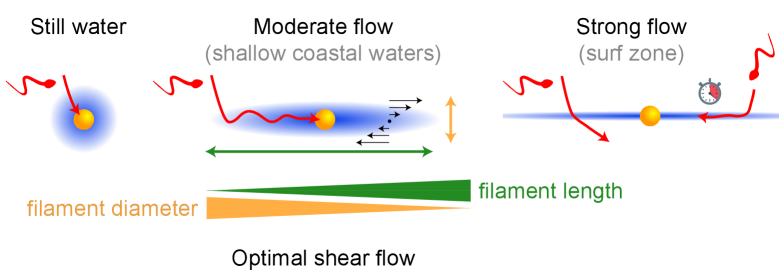
Figure 5: Proposed mechanism explaining optimal flow strength for sperm chemotaxis. Egg cells (yellow) release signaling molecules (blue) that guide sperm cells of marine species with external fertilization (red). External flows (black arrows) stretch concentration gradients into millimeter-long filaments. If sperm cells encounter such filaments, they can “surf” by chemotaxis towards the egg. In strong flows, however, sperm cells may fail to follow the filament after encounter, because the effective diameter of filaments is too small. Additionally, in very long filaments, sperm cell may not reach the egg within the sperm-egg exposure time (which is set by the lifetime of the smallest eddies for turbulent flow). Thus, it is not the total volume of the chemoattractant plume that determines fertilization success, but the geometric shape of filaments. The competition between increasing filament length, which favors sperm-egg encounters, and decreasing filament diameter, which jeopardizes filament surfing, sets an optimal flow strength that maximizes sperm-egg encounters. The optimal flow strength predicted by our theory matches physiological flow strengths in typical habitats.

In our simulations, we considered a constant sperm-egg exposure time, independent of flow strength, following the experimental protocol from [25, 38, 19, 20]. For fully developed turbulence in natural habitats, the life time of the smallest eddies sets an effective sperm-egg exposure time, as the turn-over of small-scale eddies resets local concentration fields surrounding the egg. As a consequence, the sperm-egg exposure time decreases with increasing flow strength (approximately, $t_{\text{max}}\approx 25/\alpha\sim\varepsilon^{-1/2}$, using the decay time scale of corresponding Burger vortices, see Sec. G ). This provides yet a third effect that reduces the success of sperm chemotaxis in strong turbulence. While the steady shear flow is a minimal model, we expect more realistic turbulence simulations to yield similar results at the relevant scales based on simulations with an unsteady shear flow, as shown in Fig 1A: although, the shear rate is rather large $\alpha=0.17\leavevmode\nobreak\ \text{s}^{-1}$, i.e., almost twice as large as the shear rate at the optimum, concentration filaments are only slightly bent by the rotational diffusion of the shear axis in unsteady shear flow, and we consistently find that sperm cells surf along slender concentration filaments, as exemplified in Fig 1A.

Our numerical simulations quantitatively account for previous fertilization experiments in Taylor-Couette chambers. These experiments impressively demonstrated the reduction of fertilization success at high flow rates and hinted at the existence of an optimal flow rate, which motivated our theoretical study. Our theoretical analysis highlights two subtleties in the interpretation of these early experiments, i.e., a high background concentration of chemoattractant and possibly insufficient mixing of sperm and egg cells in the absence of flow, both of which can confound an existing optimum. Nonetheless, we are indebted to this pioneering work and can now predict conditions, under which an optimal flow strength is expected. This can aid the rational design of future experiments. While a direct experimental observation of filament surfing is pending, recent 3D tracking experiments of sea urchin sperm cells navigating in axially symmetric chemoattractant landscapes gave intriguing anecdotal evidence how these cells first found the centerline of these concentration filaments and subsequently moved parallel to this centerline [15]. While our numerical simulations consider a specific mechanism of sperm chemotaxis along helical paths, our analytical theory is more general and applies in particular to any chemotaxis strategy for which the swimming direction gradually aligns to the local gradient direction. This suggests that the presence of an optimal flow strength could be a general phenomenon.

We expect that our findings of two-stage chemotactic search, comprising finding a filament and subsequent surfing along this filament, could be also relevant for foraging of bacteria and plankton: Nutrient patches are stirred by turbulent flow into networks of thin filaments, in which these organisms have to navigate for optimal uptake. Finding sinking marine snow from whose surface nutrients dissolve bears resemblance to finding egg cells which release chemoattractant. These organisms play an important role for oceanic ecosystems [42, 43, 26, 21, 44, 45, 46, 47, 48]. While our theory addresses the experimentally more accessible model system of external fertilization as employed by marine invertebrates [6], chemotaxis in external flows is relevant also for internal fertilization, where sperm cells navigate complex environments [49, 50], likely guided by both chemotaxis [5] and rheotaxis [51, 52, 53]. We emphasize that rheotaxis and chemotaxis in the presence of external flow as considered here rely on different physical mechanisms, despite formal similarities, such as active swimming upstream an external flow. While rheotaxis relies on the co-rotation of active swimmers, we found co-rotation to be dispensable for successful chemotactic navigation, with upstream swimming arising solely from chemotactic alignment to concentration filaments shaped by flow.

More generally, we characterized sperm chemotaxis in external flow as a combination of random exploration, followed by local gradient ascent, which corroborates a general paradigm for cellular and animal search behavior [54]. The minimalistic information processing capabilities of sperm cells (comparable to that of a single neuron [9]) can inspire biomimetic navigation strategies for artificial microswimmers with limited information processing capabilities intended for navigation in dynamic and disordered environments [55, 56].

Methods and Materials

The encounter probability $P_{\text{sperm:egg}}$ is computed numerically by simulating sperm trajectories $\mathbf{r}(t)$ in the presence of both a concentration field $c(\mathbf{r})$ of chemoattractant and an external fluid flow field $\mathbf{v}_{\text{ext}}(\mathbf{r})$ according to equations of motion for $\mathbf{r}(t)$, see Sec. B. These equations extend a previous, experimentally confirmed theory of sperm chemotaxis along helical paths [14, 15] by incorporating convection and co-rotation of cells by the external flow. For co-rotation, we employ Jeffery equation for prolate spheroids [30, 31] by assigning sperm cells an effective aspect ratio $g=5$. For the shear rates considered here, the effect of external flow on sperm flagellar beat patterns is negligible [57]. Each sperm cell is simulated for an exposure time $t_{\text{max}}$, which is set by protocol of the corresponding experiment, or until it hits the surface of the egg.

As external flow, we assume a simple shear flow around a freely-rotating spherical egg, see Sec. A. Throughout, we consider the co-moving frame of the egg allowing us to assume that the egg is at the origin $\mathbf{r}=\mathbf{0}$. The concentration field is established by diffusion and convection from the egg releasing chemoattractant at a constant rate. We consider the reference case of a static concentration field corresponding to a chemoattractant release time equal to exposure time $t_{\text{max}}$. Note that the exposure time $t_{\text{max}}$ may also be estimated by the decay time scale of a Burger vortex $t_{\text{max}}\sim 25/\alpha$, see Sec. H. To account for an ensemble of eggs at density $\rho_{\text{egg}}$, we consider a single egg with radius $r_{\text{egg}}$ at the origin $\mathbf{r}=\mathbf{0}$ and a spherical domain with radius $r_{\text{max}}=\left(4\pi\rho_{\text{egg}}/3\right)^{-1/3}$ and appropriate periodic boundary conditions: Initially, sperm cell positions $\mathbf{r}$ ($r_{\text{egg}}\leq\left|\mathbf{r}\right|\leq r_{\text{max}}$) and directions of the helix axis $\mathbf{h}$ are uniformly distributed, representing the distribution after initial turbulent mixing of egg and sperm cells. If sperm cells leave the simulation domain, they re-enter with random new initial conditions $\mathbf{r}$ and $\mathbf{h}$ with $\left|\mathbf{r}\right|=r_{\text{max}}$, whose distribution $P_{b}(\mathbf{r},\mathbf{h})$ is defined by the theoretical in-flux of cells due to active swimming and convection

$$P_{b}\left(\mathbf{r},\mathbf{h}\right)\sim-p_{\text{sperm}}\left(\mathbf{r},\mathbf{h}\right)\left[\left(\mathbf{v}_{\text{ext}}\left(\mathbf{r}\right)+v_{h}\mathbf{h}\right)\cdot\mathbf{e}_{r}\left(\mathbf{r}\right)\right]$$ (6)

with uniform and isotropic distribution of sperm cells $p_{\text{sperm}}\left(\mathbf{r},\mathbf{h}\right)$. In principle, co-rotation of non-spherical particles by shear flow leads to a non-uniform distribution of directions $\mathbf{h}$, see analytic solutions in Sec. F, but the effect on simulation results is negligible.

Parameters for Fig 2 were chosen to closely match conditions of A. punctuala sea urchin in their natural spawning habitat at low egg density $\rho_{\text{egg}}$ and relatively long exposure times $t_{\text{max}}$. Parameters for Figs 3 and 4 are chosen to match the experiments by Zimmer and Riffell [19, 20] and Mead and Denny [25], respectively. For further details on simulations and extensive discussion of parameters used for each scenario, see Sec. G, Sec. H. Finally, error bars for simulation results represent simple standard deviation (SD) of the corresponding binomial distribution. Error bars are smaller than symbol sizes in some cases.

Supporting Information text

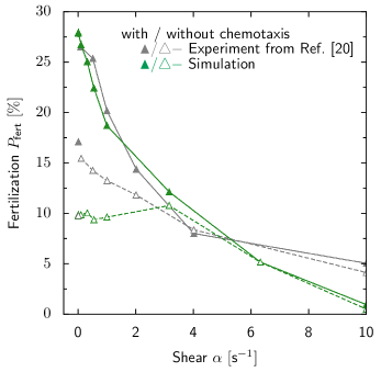
Figure A: Fertilization probability with co-rotation. Fertilization probability $P_{\text{fert}}(\alpha)$ as in Fig 3 but with simulations taking into account co-rotation (green triangles): Previous experimental data ([20], Fig. 5c) for red abalone H. rufescens with and without chemotaxis (filled gray triangles: with chemotaxis, open gray triangles: inhibited chemotaxis) and our corresponding simulations (filled green triangles: with chemotaxis, open green triangles: without chemotaxis; mean $\pm$ SD), using fertilizability $p_{\text{f}}=60\%$ in Eq. (5) as single fit parameter. Experiment and simulation again agree reasonably except for the data point without flow $\alpha=0\leavevmode\nobreak\ \text{s}^{-1}$, which corresponds to a different experimental protocol. While the simulations with co-rotation overestimate the reduction of $P_{\text{fert}}$ at high shear rate $\alpha>6\leavevmode\nobreak\ \text{s}^{-1}$, these high shear rates are less relevant for the spawning habitat of H. rufescens.

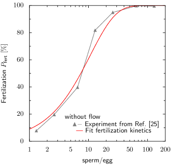
Figure B: Calibration of fertilizability without flow ($\alpha=0$). Fertilization probability $P_{\text{fert}}$ as function of the ratio $\rho_{\text{sperm}}/\rho_{\text{egg}}$ of sperm and egg density in the absence of flow $\alpha=0\leavevmode\nobreak\ \text{s}^{-1}$ from experiments with sea urchin S. purpuratus ([25], Fig. 4) (filled gray triangles) and fit of fertilization kinetics Eq. (5) (red). From the fit, we obtain $p_{\text{f}}P_{\text{sperm:egg}}\approx 9\%$ for the product of fertilizability $p_{\text{f}}$ and encounter probability $P_{\text{sperm:egg}}$. Assuming a ballistic swimmer that is captured at the egg surface (Eq. (5) with $P_{\text{sperm:egg}}(t_{\text{max}})=1-\exp(-qt_{\text{max}})$ and rate $q=\pi r_{\text{egg}}^{2}v_{h}\rho_{\text{egg}}=0.02\leavevmode\nobreak\ \text{s}^{-1}$), we find $p_{\text{f}}\approx 10\%$ for exposure time $t_{\text{max}}=120\leavevmode\nobreak\ \text{s}$ and $\rho_{\text{egg}}=1.5\cdot 10^{4}\leavevmode\nobreak\ \text{ml}^{-1}$. This value $p_{\text{f}}$ is used in Fig 4, Fig C.

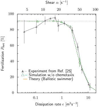
Figure C: Fertilization probability with co-rotation. Fertilization probability $P_{\text{fert}}(\alpha)$ as in Fig 4 but with simulations taking into account co-rotation of sperm cells (open green triangles): Previous measurements of fertilization probability $P_{\text{fert}}(\epsilon)$ for sea urchin S. purpuratus at strong turbulence, characterized by density-normalized dissipation rate $\epsilon$ (filled gray triangles) [25, 38] and our corresponding simulations $P_{\text{fert}}(\alpha)$ as function of shear rate $\alpha$ (open green triangles, mean $\pm$ SD) match well, using a single fit parameter $a=0.023$ that relates dissipation rate $\epsilon$ and typical shear rate $\alpha$ (with the known relationship $\alpha(\epsilon)=a\sqrt{\epsilon/\nu}$ [24, 26]). Analogous to Fig 4, the case of low shear rates is well described by the limit case of a ballistic swimmer in the absence of flow $\alpha=0\leavevmode\nobreak\ \text{s}^{-1}$ (dotted horizontal line, Eq. (5) with $P_{\text{sperm:egg}}(t)=1-\exp(-qt)$ and rate $q=\pi r_{\text{egg}}^{2}v_{h}\rho_{\text{egg}}$). The fertilizability $p_{\text{f}}=10\%$ is obtained from an independent experiment [25], see Fig B. From the experimental protocol, we estimate a high background concentration $c_{\text{bg}}=500-4000\leavevmode\nobreak\ \text{nM}$ of chemoattractant, which renders sperm chemotaxis ineffective.

A Shear flow around freely-rotating egg and minimal case of ballistic swimmer

For all simulations (except Fig 1A), we use a simple shear flow $\alpha y\,\mathbf{e}_{x}$ as idealized paradigm for small-scale turbulence. At the relevant shear rates $\alpha$ and typical egg radii $r_{\text{egg}}\sim 100\leavevmode\nobreak\ \mu\text{m}$, the Reynolds number $\text{Re}=\alpha r_{\text{egg}}^{2}/\nu\leq 0.1$ is sufficiently small to justify the use of the analytical Stokes equation for viscous flow $\mathbf{v}_{\text{ext}}(\mathbf{r})$. Throughout, we consider the co-moving frame of the egg allowing us to assume that the egg is at the origin $\mathbf{r}=\mathbf{0}$. We introduce dimensionless coordinates $\hat{\mathbf{r}}=\mathbf{r}/r_{\text{egg}}$ and the dimensionless flow field $\mathbf{\hat{v}}_{\text{ext}}\left(\mathbf{\hat{r}}\right)=\frac{2\mathbf{v}_{\text{ext}}\left(\mathbf{r}\right)}{\alpha r_{\text{egg}}}$. The components of this flow field read ([58], Eq. (12))

$$\hat{v}{}_{\text{ext},x} =2\hat{y} -\hat{y}\left(\left[1+\hat{\Omega}\right]\hat{r}^{-3}+\hat{r}^{-5}\right) -5\hat{x}^{2}\hat{y}\left(\hat{r}^{-5}-\hat{r}^{-7}\right)$$ (S1)

$$\hat{v}{}_{\text{ext},y} = \phantom{+}\hat{x}\left(\left[1+\hat{\Omega}\right]\hat{r}^{-3}-\hat{r}^{-5}\right) -5\hat{x}\hat{y}^{2}\left(\hat{r}^{-5}-\hat{r}^{-7}\right)$$

$$\hat{v}{}_{\text{ext},z} = -5\hat{x}\hat{y}\hat{z}\left(\hat{r}^{-5}-\hat{r}^{-7}\right)$$

where no-slip boundary conditions on the surface $\left|\mathbf{\hat{r}}\right|=1$ of the freely-rotating spherical egg are assumed. The egg rotates according to the undisturbed flow vorticity with the dimensionless rotation rate $\hat{\Omega}=-1$, corresponding to an rotation of the egg with angular velocity $\mathbf{\Omega}=-\frac{\alpha}{2}\mathbf{e}_{z}$.

It is instructive to consider a ballistic swimmer in the above flow field $\mathbf{v}_{\text{ext}}$ as a reference for the analysis of more complicated cases, such as swimmers performing chemotaxis. For instance, without flow or chemotaxis, sperm cells are considered to swim along a straight helix with helix radius $r_{0}$ much smaller than the egg radius. These sperm trajectories are well approximated by a ballistic swimmer moving along the helix axis $\mathbf{h}$ with net swimming speed $v_{h}$. If the ballistic swimmers and the target eggs (with density $\rho_{\text{egg}}$) are uniformly distributed, the steady-state rate $q$ at which a swimmer hits an egg is given by $q=\pi(r_{\text{egg}}+r_{0})^{2}v_{h}\rho_{\text{egg}}\approx\pi r_{\text{egg}}^{2}v_{h}\rho_{\text{egg}}$. If ballistic swimmers become trapped at the egg on encounter, this corresponds to the encounter probability $P_{\text{sperm:egg}}(t)=1-\exp(-qt)$ (and fertilization probability $P_{\text{fert}}$ according to fertilization kinetics, see Eq. (5)). If ballistic swimmers are additionally convected by an external fluid flow field $\mathbf{v}_{\text{ext}}$, we can characterize $q$ (and thus $P_{\text{sperm:egg}}$ and $P_{\text{fert}}$) in terms of an universal curve: We introduce the dimensionless parameter $f=\frac{\alpha r_{\text{egg}}}{2v_{h}}$, which compares shear rate to net swimming speed. The combined velocity field of active swimming and fluid flow is now

$$\mathbf{v}_{\text{ext}}\left(\mathbf{r}\right)+v_{h}\mathbf{h}=v_{h}\left(f\mathbf{\hat{v}}_{\text{ext}}\left(\mathbf{\hat{r}}\right)+\mathbf{h}\right)=v_{h}\mathbf{\hat{u}}\left(\mathbf{\hat{r}},f,\mathbf{h}\right)\ .$$ (S2)

Note that without co-rotation, $\mathbf{h}$ does not change. Thus, for any $\mathbf{h}$, all possible velocity fields $\mathbf{\hat{u}}$ are given by a single one-parameter family parametrized by $f$. For each of these fields, the dimensionless rate of swimmers $\hat{q}\left(f,\mathbf{h}\right)$ reaching the egg from $\left|\mathbf{\hat{r}}\right|\gg 1$ specifies the actual rate $q$ for any set of parameters $\alpha,r_{\text{egg}},v_{h},\rho_{\text{egg}}$ with the same parameter $f$ by

$$q\left(\alpha,r_{\text{egg}},v_{h},\mathbf{h}\right)=\hat{q}\left(f,\mathbf{h}\right)r_{\text{egg}}^{2}v_{h}\rho_{\text{egg}}\ .$$ (S3)

We obtain a universal curve for $q$ by computing $\hat{q}(f,\mathbf{h})$ numerically for all $f$ and $\mathbf{h}$ and average $\hat{q}(f)=\left<\hat{q}(f,\mathbf{h})\right>_{\mathbf{h}}$ over all directions $\mathbf{h}$, see Fig 4 for corresponding $P_{\text{fert}}$. A prominent feature of the universal rate is that it vanishes at large shear rates $\hat{q}\left(f\to\infty\right)\to 0$. In the absence of flow $\alpha=0$, we have $\hat{q}\left(f=0\right)=\pi$.

We compute the universal rate $\hat{q}$ efficiently by integrating a uniform grid of initial conditions on the surface of the egg, with $\left|\mathbf{\hat{r}}\right|=1$ at $\hat{t}=0$, backwards in time according to the velocity field $\mathbf{\hat{u}}$. Each initial condition is integrated until it either returns to the egg $\left|\mathbf{\hat{r}}\right|(\hat{t})=1$ (fail) or leaves the outer boundaries $\mathbf{\hat{r}}(\hat{t})=\hat{r}_{\text{max}}$ (success) with $\hat{r}_{\text{max}}\gg 1$. As the flow is volume conserving, the results are independent of the choice of the outer boundary $\hat{r}_{\text{max}}$, as long as $\hat{r}_{\text{max}}$ is sufficiently large to ensure the absence of closed orbits beyond it. We choose $\hat{r}_{\text{max}}=4$ as numerics show that the in- and outflow on this sphere differs only by $4\%$ between the Stokes flow around the freely-rotating sphere and the undisturbed simple shear flow, for which it is known no closed orbits exist. Based on the intersections with the outer boundary, the flow reaching the egg is interpolated. This is done for a grid of swim directions $\mathbf{h}$. For efficiency, we exploit the symmetries of the Stokes flow $\mathbf{\hat{v}}_{\text{ext}}\left(\hat{x},\hat{y},\hat{z}\right)\cdot\left(h_{x}\mathbf{e}_{x}+h_{y}\mathbf{e}_{y}+h_{z}\mathbf{e}_{z}\right)=\mathbf{\hat{v}}_{\text{ext}}\left(\hat{x},\hat{y},-\hat{z}\right)\cdot\left(h_{x}\mathbf{e}_{x}+h_{y}\mathbf{e}_{y}-h_{z}\mathbf{e}_{z}\right)=\mathbf{\hat{v}}_{\text{ext}}\left(-\hat{x},-\hat{y},\hat{z}\right)\cdot\left(-h_{x}\mathbf{e}_{x}-h_{y}\mathbf{e}_{y}+h_{z}\mathbf{e}_{z}\right)$; thus, it is sufficient to consider $h_{z}\geq 0$ and $h_{y}\geq 0$, respectively.

B Equations of motion for navigating sperm cells

We simulate the swimming path $\mathbf{r}(t)$ of a sperm cell in a concentration field $c(\mathbf{r})$ of chemoattractant in the presence of an external fluid flow field $\mathbf{v}_{\text{ext}}(\mathbf{r})$. For this, we extend a previous theory of chemotaxis of marine sperm cells along helical paths [14, 59, 4, 15] by incorporating convection and co-rotation by flow: The sperm cell is described in terms of the time-dependent center position $\mathbf{r}(t)$, averaged over one flagellar beat cycle, and the set of ortho-normal vectors $\mathbf{e}_{1}(t),\mathbf{e}_{2}(t),\mathbf{e}_{3}(t)$ of the co-moving coordinate frame, where the vector $\mathbf{e}_{1}(t)$ points in the direction of active swimming with speed $v_{0}$. The equations of motion read

$$\dot{\mathbf{r}} =v_{0}\mathbf{e}_{1}+\mathbf{v}_{\text{ext}}(\mathbf{r}(t))\ ,$$ (S4)

$$\dot{\mathbf{e}}_{i} =\left(\mathbf{\Omega}_{\text{h}}+\mathbf{\Omega}_{\text{f}}\right)\times\mathbf{e}_{i}\qquad i=1,2,3\ ,$$

The two angular velocities, $\mathbf{\Omega}_{\text{h}}$ and $\mathbf{\Omega}_{\text{f}}$, describe the rotation of the coordinate frame due to helical chemotaxis and external flow, respectively. For Eq. (S4) a constant swim speed is assumed and motility noise is neglected; the persistence length of sperm swimming paths in the absence of chemoattractant cues was estimated as $3-25\leavevmode\nobreak\ \text{mm}$ [33] which validates this assumption. Note that Eq. (S4) is also valid for time-dependent concentration and flow fields. Note further that the quantitative comparison of the two angular velocities in Eq. (S4) already suggests that the rotation due to external flow is negligible, as the rate of change due to external flow $\Omega_{\text{f}}\sim\alpha=0-1\leavevmode\nobreak\ \text{s}^{-1}$ (see Eq. (S8)) is always smaller than due to the helical motion $\Omega_{\text{h}}\sim\tau_{0}v_{0}=3-13\leavevmode\nobreak\ \text{s}^{-1}$ (see Eq. (S5) and parameters in Table A).

Without external flow or chemotaxis, cells swim along a helical path with constant path curvature $\kappa(t)=\kappa_{0}$ and torsion $\tau(t)=\tau_{0}$. The angular velocity $\mathbf{\Omega}_{\text{h}}$ is defined by the Frenet-Serret equations

$$\mathbf{\Omega}_{\text{h}}(t)=v_{0}\left[\tau(t)\mathbf{e}_{1}(t)+\kappa(t)\mathbf{e}_{3}(t)\right]\ ,$$ (S5)

where the coordinate frame $\mathbf{e}_{1},\mathbf{e}_{2},\mathbf{e}_{3}$ corresponds to the Frenet-Serret frame of $\mathbf{r}(t)$, i.e., tangent, normal and bi-normal vector. During chemotactic steering, sperm cells dynamically regulate curvature $\kappa(t)$ and torsion $\tau(t)$ of active swimming according to the output $a(t)$ of a chemotactic signaling system

$$\kappa(t) =\kappa_{0}-\rho\kappa_{0}(a-1)\ ,$$ (S6)

$$\tau(t) =\tau_{0}+\rho\tau_{0}(a-1)\ .$$

Here, the sensori-motor gain factor $\rho$ characterizes the amplitude of chemotactic steering responses. The chemotactic signaling system takes as input the local concentration $c(\mathbf{r}(t))$ at the position of the cell

$$\mu\dot{a} =p\left[c_{b}+c(\mathbf{r}(t))\right]-a\ ,$$ (S7)

$$\mu\dot{p} =p\left(1-a\right)\ .$$

This minimal signaling system comprises sensory adaption with sensitivity threshold $c_{b}$ and relaxation with time scale $\mu$ to a rest state $a=1$ for any constant stimulus $c(\mathbf{r}(t))=c_{0}$. The variable $p$ describes an dynamic sensitivity which is regulated down when the stimulus is high, or regulated up when the stimulus is low (a loose analogy would be that $p$ corresponds to the opening of our eye’s pupils as adaption to brightness). In principle, $p$ and $a$ could have different time-scales [14]. However, equal time-scales automatically ensure that the phase-lag between small-amplitude oscillations of the input signal $c(\mathbf{r}(t))$ and resulting oscillation of the output signal $a(t)$ attains the value $\pi/2$ optimal for helical chemotaxis [59]. This special case is sufficient for the purpose of a minimal model. The gain factor $\rho$ sets the rate of chemotactic steering. While $\rho$ could depend on the chemotactic signal by a feedback mechanism  [17], we assume here a constant gain factor $\rho=5$ for simplicity. The values of all parameters are listed and discussed in Sec. G.

We approximate the angular velocity $\mathbf{\Omega}_{\text{f}}$ for co-rotation by external flow using the Jeffery equation for a small prolate spheroid with major axis along $\mathbf{e}_{1}$ [30, 31]

$$\mathbf{\Omega}_{\text{f}}(\mathbf{r}) =\frac{1}{2}\mathbf{\omega}(\mathbf{r})+G\mathbf{e}_{1}\times\left[\mathbf{E}(\mathbf{r})\cdot\mathbf{e}_{1}\right]\ ,$$ (S8)

$$\mathbf{\omega}(\mathbf{r}) =\bm{\nabla}\times\mathbf{v}_{\text{ext}}(\mathbf{r})\ ,$$

$$\mathbf{E}(\mathbf{r}) =\frac{1}{2}\left[\bm{\nabla}\otimes\mathbf{v}_{\text{ext}}(\mathbf{r})+\left(\bm{\nabla}\otimes\mathbf{v}_{\text{ext}}(\mathbf{r})\right)^{T}\right]$$

with the flow vorticity $\mathbf{\omega}$, the strain rate tensor $\mathbf{E}$, and a geometric factor $G=\frac{g^{2}-1}{g^{2}+1}$, which depends on the aspect ratio $g\geq 1$ of major to minor axis of the spheroid. Together with Eq. (S4), Eq. (S8) describes the cell rotation due the flow, i.e., The first term in the first line of Eq. (S8) describes rotation of a spherical body due to flow vorticity and the second term the correction for non-sperical bodies that can be approximated as spheroids. For a swimming sperm cell, we take the swim direction $\mathbf{e}_{1}$ as effective major axis, and employ an effective aspect ratio, $g=5$, reflecting the ratio of the length of the flagellum and a typical beat amplitude [19]. Note that in general instead of $\mathbf{e}_{1}$, the major axis could be any co-moving vector.

We numerically integrate the equations of motion, i.e., Eqs. (S4,S7), using an Euler scheme with fixed small time step $dt$. For efficient computation, Rodrigues rotation formula [60] with respect to the co-moving coordinate frame is used to integrate $\mathbf{e}_{1},\mathbf{e}_{2},\mathbf{e}_{3}$, resulting in faster computation compared to the algorithm used in [17].

C Analysis of concentration filaments

Turbulent flows cause turbulent mixing of diffusing chemicals and generate filamentous concentration fields. As a minimal model, we simplify the turbulent flow and the filamentous concentration field by the case of a simple shear flow. We consider a spherical egg located at the origin $\mathbf{r}=\mathbf{0}$ releasing chemoattractant with diffusion coefficient $D$ at a constant rate $\dot{Q}$ in the presence of shear flow $\mathbf{v}_{\text{ext}}(\mathbf{r})$ given by Eq. (S1). We compute the time-dependent concentration field $c(\mathbf{r},t)$ of chemoattractant numerically using Lagrangian particle tracking, see Sec. G. We empirically find that the far-field at distances $r\gg r_{\text{egg}}$ is well approximated by a generic profile, see Fig 1B for illustration,

$$c(\mathbf{r},t)=c_{0}\exp\left(-k\left|x\right|\right)\exp\left(-\frac{\left(y-y_{0}\right)^{2}/a_{y}^{2}+z^{2}}{2\sigma^{2}}\right)\ ,$$ (S9)

which describes a concentration filament with time-dependent parameters $c_{0}(t)$, $k(t)$, $a_{y}$, as well as time- and position-dependent variance and midline profiles $\sigma(x,t)$ and $y_{0}(x,t)$, respectively. This formula for the concentration filament is consistent with results obtained using the analytic solution for an instantaneous point source in a shear flow $\alpha y\,\mathbf{e}_{x}$, see below. We present and discuss scaling laws for the parameters in the following. While these dependencies are not explicitly required for our theory, they demonstrate the universality of our theory. Finally, we use these scaling laws to quantify how the filaments become longer and thinner with increasing shear rate $\alpha$.

From numerical simulations, we empirically find the following scaling laws of the parameters from Eq. (S9)

$$k\left(t\right) \sim t^{-\delta_{k}}\ , \delta_{k} =1.5\text{ -- }1.6$$ (S10)

$$c_{0}\left(t\right) \sim t^{-\delta_{c_{0}}}\ , \delta_{c_{0}} =1.6\text{ -- }1.8$$ (S10b)

$$\sigma^{2}\left(x,t\right) =2D\,t_{0}\left(x,t\right)\ , t_{0} \sim t$$ (S10c)

$$t_{0}\left(x,t\right) \ =p_{0,t_{0}}\left(t\right)+p_{1,t_{0}}\left(t\right)\left|x\right|+p_{2,t_{0}}\left(t\right)\left|x\right|^{2},$$ (S10d)

$$y_{0}\left(x,t\right) =\mathrm{sgn}\left(x\right)p_{0,y_{0}}\left(t\right)+p_{1,y_{0}}{}t^{-\delta_{y_{0}}}x\ , \delta_{y_{0}} =0.9\text{ -- }1.0$$ (S10e)

$$p_{1,y_{0}}{} =(1\text{ -- }1.4)\alpha^{-\delta_{y_{0}}}\ ,\qquad\qquad a_{y} =0.5\text{ -- }0.6$$ (S10f)

where all parameters except $p_{2,t_{0}}$ are positive. Note that in a turbulent flow the time $t$ in which the filament is formed may scale with the Kolmogorov time $t\sim\tau_{\text{Kol}}$; in this case $\sigma$ would scale as the Batchelor length $\sigma\sim\sqrt{D\tau_{\text{Kol}}}$. We also found power-law dependencies for the coefficients $p_{0,t_{0}}(t)$, $p_{1,t_{0}}(t)$, and $p_{2,t_{0}}(t)$. The factor $a_{y}$ appears to be constant for sufficiently large $t$. These numerical observations become plausible by analysis of a point source in shear flow. The Fokker-Planck equation for this case can be written in dimensionless form

$$\partial_{t}c=-\alpha y\,\partial_{x}c+D\bigtriangleup c\,+\,\dot{Q}\,\delta(\mathbf{r})\Rightarrow\partial_{\check{t}}\check{c}=-\check{y}\,\partial_{\check{x}}\check{c}+\bigtriangleup\check{c}\,+\,\delta(\check{\mathbf{r}})$$ (S11)

by using the Batchelor scale $\sqrt{D\tau_{\text{Kol}}}\sim\sqrt{D/\alpha}$ to re-scale to dimensionless coordinates

$$\check{x}=x\sqrt{\frac{\alpha}{D}}\ ,\quad\check{y}=y\sqrt{\frac{\alpha}{D}}\ ,\quad\check{t}=t\alpha\ ,\quad\check{c}=c\sqrt{\frac{D^{3}}{\alpha}}\frac{1}{\dot{Q}}$$ (S12)

with shear rate $\alpha$, and release rate $\dot{Q}$ of the source (i.e. $\iiint_{-\infty}^{\infty}\mathrm{d}^{3}r\,c(\mathbf{r},t)=\dot{Q}\,t$). Consequently, the solution $\check{c}\left(\mathbf{\check{r}},\check{t}\right)$ of this equation can be re-scaled to the solution $c(\mathbf{r},t)$ for any set of parameters $\alpha,D,\dot{Q}$. For the above form of the far-field of the filament, this implies that the parameters $\delta_{k}$, $\delta_{c_{0}}$, $p_{1,y_{0}}$ and $p_{2,t_{0}}$ are universal as they are invariant under the re-scaling Eq. (S12). The analytical solution for the dimensionless concentration $\check{c}$ reads ([61], Eq. (18))

$$\check{c}\left(\mathbf{\check{r}},\check{t}\right)=\int\limits_{0}^{\check{t}}\mathrm{d}\check{s}\,\check{G}(\mathbf{\check{r}},\check{s})$$ (S13)

with Greens function $\check{G}$, i.e., the solution for an instantaneous source at the origin ([62], Eq. (26))

$$\check{G}(\mathbf{\check{r}},\check{t})=\frac{\exp\left[-\frac{\left(\check{x}-\frac{1}{2}\check{y}\check{t}\right)^{2}}{4\check{t}\left(1+\frac{1}{12}\check{t}^{2}\right)}-\frac{\check{y}^{2}+\check{z}^{2}}{4\check{t}}\right]}{\left(4\pi\check{t}\right)^{\frac{3}{2}}\sqrt{1+\frac{1}{12}\check{t}^{2}}}\ .$$ (S14)

While the integral Eq. (S13) cannot be solved analytically, it explains the empirical scaling for the parameters in Eq. (S9) heuristically: It is reasonable to assume that for any $\check{x}$, the parameter $\check{y}_{0}(\check{t})$ is close to the point $\check{y}_{\text{max}}$ of the maximal concentration of $\check{G}(\check{\mathbf{r}},\check{t})$. From $\partial_{\check{y}}\check{G}(\check{x},\check{y},\check{z}=0,\check{t})|_{\check{y}=\check{y}_{\text{max}}}=0$, it follows (for $\check{t}>\sqrt{3}$)

$$\check{y}_{0}(\check{x},\check{t})\approx\check{y}_{\text{max}}(\check{x},\check{t})=\frac{3\check{t}\check{x}}{2(\check{t}^{2}+3)}\Rightarrow p_{1,y_{0}}{}\approx\frac{3}{2}\check{t}^{-1}$$ (S15)

in accordance with the fitted power-law.

The power law $c_{0}(t)\sim t^{-\frac{3}{2}}$, as suggested by numerics, is plausible since $\check{G}\left(\mathbf{0},\check{s}\gg 1\right)\sim\check{s}^{-\frac{5}{2}}$, which implies $\check{c}\left(\mathbf{0},\check{t}\gg 1\right)\sim\int_{0}^{\check{t}}\mathrm{d}\check{s}\,\check{s}^{-\frac{5}{2}}\sim\check{t}^{-\frac{3}{2}}$.

We introduce the concentration $\check{c}_{\text{max}}$ at the centerline of the filament $\check{c}_{\text{max}}\left(\check{x},\check{t}\right)=\check{c}\left(\check{x},\check{y}_{0}\left(\check{x},\check{t}\right),\check{z}=0\right)$. We make the ansatz $\check{c}_{\text{max}}\left(\check{x},\check{t}\right)=\check{c}_{0}(\check{t})\exp\left(-\check{k}\left(\check{t}\right)\left|\check{x}\right|\right)$ and derive a power-law for $\check{k}(\check{t})$ in the following. We expect that $\check{c}_{\text{max}}$ scales proportional to the summed contributions of the Greens functions at the time-dependent centerline, hence we estimate (assuming $\check{t}\gg 1$, we approximate $\check{t}^{2}+3\to\check{t}^{2}$, $1+\check{t}^{2}/12\to\check{t}^{2}/12$ in $\check{G}$)

$$\check{c}_{\text{max}}\left(\check{x},\check{t}\right)\sim\int\limits_{0}^{\check{t}}\mathrm{d}\check{s}\,\check{G}(\check{x},\check{y}_{0}(\check{x},\check{s}),\check{z}=0,\check{s})\sim\frac{\mathrm{erfc}{\left(\sqrt{\frac{3}{4\check{t}^{3}}}\check{x}\right)}}{6\pi\check{x}}\ .$$ (S16)

We are interested in the shape of the concentration filament up to a maximal distance $\check{x}_{\text{max}}$ at which the concentration at the centerline decayed to a fraction $\iota$ of $\check{c}_{0}$, $\check{c}_{\text{max}}(\check{x}_{\text{max}},\check{t})=\iota c_{0}(\check{t})$. Any asymptotic tails beyond this distance will likely not be relevant for chemotaxis. Since the decay of $\check{c}_{\text{max}}$ as function of $\check{x}$ is dominated by the numerator in Eq. (S16), the distance $\check{x}_{\text{max}}$ has a time-dependency $\check{x}_{\text{max}}\left(\check{t}\right)\sim\check{t}^{\frac{3}{2}}$ according to the argument of the complementary error-function $\mathrm{erfc}$. Using Eq. (S16), we estimate the time-dependency of $\check{k}(\check{t})$ from

$$-\check{k}(\check{t})\check{x}=\ln\left(\frac{\check{c}_{\text{max}}(\check{x})}{\check{c}_{0}}\right)\sim\ln\left(\frac{\mathrm{erfc}{a}}{a}\right)\sim\ln\mathrm{erfc}\left(a\right)\sim-a\ ,$$ (S17)

where we introduced $a(\check{x},\check{t})=\sqrt{3/4}\ \check{t}^{-\frac{3}{2}}\check{x}$. The crucial point is that for $0\leq\check{x}\leq\check{x}_{\text{max}}(\check{t})$, the variable $a$ varies only in a finite interval $0\leq a\leq a_{\text{max}}$ with upper bound $a_{\text{max}}=a(\check{x}_{\text{max}}(\check{t}),\check{t})\sim\check{t}^{-\frac{3}{2}}\check{x}_{\text{max}}(\check{t})$ independent of time $\check{t}$. This allows us to approximate $\ln\mathrm{erfc}\left(a\right)$ by its Taylor expansion for small $a\ll 1$ in the last step of Eq. (S17). We conclude $\check{k}\left(\check{t}\right)\sim a_{\text{max}}/\check{x}_{\text{max}}(\check{t})\sim\check{t}^{-\frac{3}{2}}$, as suggested by numerics.

From the above considerations follows that for a constant exposure time $t_{\text{max}}$ the filaments become longer and thinner with increasing shear rate $\alpha$: From Eq. (S12) follows for the dimensionless exposure time $\check{t}_{\text{max}}=t_{\text{max}}\alpha$ and thus the exponent $\check{k}$ of the dimensionless version of Eq. (S9) scales with $\check{k}\sim(t_{\text{max}}\alpha)^{-\frac{3}{2}}$, which implies according to $\check{k}\check{x}=kx$ a scaling of the effective decay length

$$1/k\sim\alpha\sqrt{Dt_{\text{max}}^{3}}\ .$$ (S18)

This means that for constant exposure time $t_{\text{max}}$ the effective length of the filament increases with shear rate $\alpha$. Analogously, from $\check{\sigma}\sim\sqrt{t_{\text{max}}\alpha}$ and $\check{c}_{0}\sim\left(t_{\text{max}}\alpha\right)^{-\frac{3}{2}}$ follows with the re-scaling Eq. (S12) for the effective decay length $\sigma$ away from the center of the filament and the base concentration $c_{0}$

$$\sigma \sim\sqrt{Dt_{\text{max}}}$$ (S19)

$$c_{0} \sim\frac{\dot{Q}}{\alpha\left(Dt_{\text{max}}\right)^{\frac{3}{2}}}\ .$$

The combination of the effective decay length $\sigma$ being independent of $\alpha$ and the base concentration $c_{0}$ decreasing with increasing $\alpha$ means that the effective width of the filament decreases with increasing $\alpha$.

D Chemotactic navigation within filament

We derive an effective equation of motion for chemotactic navigation within a typical concentration filament. For simplicity, we initially ignore interaction with the flow and assume that the motion is effectively two-dimensional, i.e., in the $xy$-plane. Additionally, we employ a two-dimensional version of Eq. (S9) for the concentration filament, setting $a_{y}=1$,

$$c(x,y,t)=c_{0}\exp\left(-k\left|x\right|\right)\exp\left(-\frac{(y-y_{0})^{2}}{2\sigma^{2}}\right)\ .$$ (S20)

We introduce the centerline $\mathbf{r}_{h}(t)=(x(t),y(t),0)$ of the helical swimming path $\mathbf{r}(t)$, with $\dot{\mathbf{r}}_{h}=v_{h}\mathbf{h}$. From a previously established equation for $\mathbf{r}_{h}$ [14, 59], we have

$$\dot{x} =v_{h}\cos\left(\varphi\right)\ ,\qquad\dot{y}=v_{h}\sin\left(\varphi\right)\ ,$$ (S21)

$$\dot{\varphi} =-v_{\varphi}\frac{\left|\bm{\nabla}c\right|}{c+c_{b}}\sin\Psi\ ,\qquad\Psi=\sphericalangle\left(\bm{\nabla}c,\mathbf{h}\right)\ ,$$

describing the alignment of the helix axis $\mathbf{h}$ with the local gradient $\bm{\nabla}c(\mathbf{r}_{h}(t))$ of a concentration field $c(\mathbf{r})$. The first equation corresponds to ballistic motion along the helix axis $\mathbf{h}(\varphi)=\cos\varphi\ \mathbf{e}_{x}+\sin\varphi\ \mathbf{e}_{y}$ with net swimming speed $v_{h}=v_{0}\tau_{0}/\sqrt{\kappa_{0}^{2}+\tau_{0}^{2}}$. The second equation describes chemotactic turning of the orientation angle $\varphi$, where $\Psi$ denotes the angle enclosed by $\mathbf{h}$ and the local gradient $\bm{\nabla}c(\mathbf{r}_{\mathbf{h}}(t))$. Here, $c_{b}$ denotes the adaption threshold and $v_{\varphi}$ the chemotactic turning speed, $v_{\varphi}=\rho v_{h}\kappa_{0}^{2}/\left(\kappa_{0}^{2}+\tau_{0}^{2}\right)$, $v_{\varphi}>0$, with the gain factor $\rho$ and helix parameters $\kappa_{0}$, $\tau_{0}$. We apply this general theory, Eq. (S21), to the filamentous profile Eq. (S20) and obtain a single dimensionless ODE

$$\ddot{Y}=\big{(}\underbrace{-\dot{X}^{2}Y}_{\sim\text{oscillator}}+\underbrace{\text{sgn}\left(X\right)\ \gamma\dot{X}\dot{Y}}_{\sim\text{damping}}\big{)}\underbrace{\frac{c}{c+c_{b}}}_{\sim\text{dimmer switch}}$$ (S22)

with $\dot{X}^{2}+\dot{Y}^{2}=1$, $\dot{X}\neq 0$ and a single dimensionless parameter

$$\gamma=k\sigma\sqrt{\frac{v_{\varphi}}{v_{h}}}=k\sigma\sqrt{\frac{\rho\kappa_{0}^{2}}{\kappa_{0}^{2}+\tau_{0}^{2}}}\ .$$ (S23)

Here, we introduce a characteristic time-scale $\tau$,

$$\tau=\sqrt{\frac{\sigma}{v_{\varphi}}\cdot\frac{\sigma}{v_{h}}}\ ,$$ (S24)

as well as re-scaled coordinates $Y(T)=\left(y(t)-y_{0}\right)/L$, $X(T)=x(t)/L$, $L=v_{h}\tau$. Dots denote differentiation with respect to re-scaled time $T=t/\tau$, e.g., $\dot{Y}=\mathrm{d}Y\,/\mathrm{d}T\,$. The time scale $\tau$ is the geometric mean of a characteristic time-scale $\sigma/v_{\varphi}$ of chemotactic steering and a typical time $\sigma/v_{h}$ for traversing the cross-sectional width $\sigma$ of the filament if steering was absent. We have an equation for $X$ analogous to Eq. (S22) (which requires $\dot{Y}\neq 0$ and covers the case $\dot{X}=0$),

$$\ddot{X}=\left(\dot{X}\dot{Y}Y-\text{sgn}\left(X\right)\ \gamma\dot{Y}^{2}\right)\frac{c}{c+c_{b}}\ .$$ (S25)

The factor $c/(c+c_{b})$ in the effective equations of motion, Eqs. (S22, S25), represents a ‘dimmer switch’ that attenuates chemotactic navigation at low concentration $c$. Thus, it is reasonable to define the filament as the region where $c(\mathbf{r})\geq c_{b}$. In the following, we focus on the dynamics within the filament and approximate $c/(c+c_{b})\approx 1$.

The effective equation of motion, Eq. (S22), describes a damped, non-linear oscillator: The first term $\dot{X}^{2}Y$ originates from the perpendicular component $\bm{\nabla}_{\perp}c=\left(\mathbf{e}_{y}\cdot\bm{\nabla}c\right)\mathbf{e}_{y}$ of the concentration filament and governs the observed oscillations of sperm cells around the centerline $Y=0$ of the filament. Heuristically, these oscillations result from sperm cells slowly aligning their helix axis $\mathbf{h}$ parallel to $\bm{\nabla}_{\perp}c$ while approaching $Y=0$. At $Y=0$, $\bm{\nabla}_{\perp}c$ changes its direction, yet sperm cells overshoot due to their finite chemotactic turning speed $v_{\varphi}<\infty$, before they eventually make a ‘U-turn’. The second term $\text{sgn}\left(X\right)\gamma\dot{X}\dot{Y}$ in Eq. (S22) originates from the exponential decay of concentration along the centerline of the filament and changes the amplitude of the oscillation. In particular, for $\text{sgn}\left(X\dot{X}\right)<0$, i.e., sperm cells surfing towards the egg, the oscillation is damped, whereas for $\text{sgn}\left(X\dot{X}\right)>0$, i.e., sperm cells surfing away from the egg, it is amplified. This increase in amplitude can cause sperm cells that are surfing away from the egg to eventually turn around, redirecting them towards the egg. A linear stability analysis of Eq. (S22) around the case of a non-oscillating trajectory $\left(Y,\dot{Y}\right)=(0,0)$ yields the eigenvalues $\omega_{1,2}$ of the Jacobian of the linearization,

$$\omega_{1,2}=\zeta\pm\mathrm{i}\sqrt{1-\zeta^{2}}\ ,\qquad\zeta=\text{sgn}\left(X\dot{X}\right)\frac{\gamma}{2}\ ,$$ (S26)

which define a harmonic oscillator with dimensionless damping ratio $\zeta$ and dimensionless oscillation frequency $\sqrt{1-\zeta^{2}}$. This analytic result agrees with full simulations of helical chemotaxis in three-dimensional space, see Fig D.

Note that the predicted exponential decay of oscillation amplitude, $\exp\left(\zeta T\right)=\exp\left(\gamma/2\cdot t/\tau\right)$, is independent of $x$ since $\gamma/\tau$ is independent of $\sigma^{2}(x)$. Interestingly, both for Eq. (S22) and full simulations, the angle at which trajectories intersect the centerline $Y=0$ of the concentration filament is essentially independent of the angle at which they first entered the filament at $Y(c=c_{b})$, provided $Y(c=c_{b})$ is sufficiently large: For smaller $Y(c=c_{b})$, i.e., outer and thus thinner parts of the filament, trajectories will simply pass through the filament, unable to execute a successful turn before they have left the filament again. As the width of the filament decreases away from the egg, this implies that filament surfing will be operative, at most, up to a maximal distance from the egg (which depends on the entry angle), characterized by $p_{\text{in}}$. If we account for convection by shear flow $\mathbf{v}_{\text{ext}}=\alpha y\,\mathbf{e}_{x}$, Eq. (S25) changes to $\dot{X}\to\dot{X}+\alpha\tau(Y+y_{0}(X)/L)$. Note that due to $\text{sgn}\left(y_{0}(x)\right)=\text{sgn}\left(x\right)$, sperm cells that surf within the filament towards the egg swim on average against the external flow.

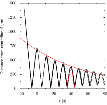
Figure D: Surfing along filaments can be described as damped oscillation. Distance $d=\sqrt{(y-y_{0})^{2}+z^{2}}$ from the centerline of concentration filament Eq. (S9) superimposed for $n=9$ sperm trajectories simulated according to Sec. B (black). Trajectories are shown after they entered the surface of the concentration filament, defined by $c(\mathbf{r}(t))=c_{b}$, and shifted in time to align the first oscillation peak at $t_{0}=0$. Remarkably, all trajectories display stereotypic oscillations that overlap perfectly, despite the fact that trajectories entered the filament at different $x$-positions and initial direction angles. The observed damped oscillation are well reproduced by a minimal analytical theory for the centerline of the helical swimming path, which predicts damping ratio and oscillation period (dashed red line, see Eq. (S26)). Parameters as in Fig 1B, corresponding to A. punctuala.

E Minimal theory for sperm-egg-encounter probability

We provide an estimate for the encounter probability $P_{\text{sperm:egg}}$, building on the effective equation of motion of the helix axis derived in Sec. D. The fertilization probability $P_{\text{fert}}$ is obtained then from $P_{\text{sperm:egg}}$ using fertilization kinetics, Eq. (5). For $P_{\text{sperm:egg}}$, we decompose the search problem for the egg into an outer search problem of finding the concentration filament and an inner search problem of surfing along the filament. We obtain (exploiting the symmetry between the two branches of the filament for $x<0$ and $x>0$)

$$P_{\text{sperm:egg}}\approx 2\int\limits_{0}^{r_{\text{max}}}\mathrm{d}x\,p_{\text{in}}(x,t_{\text{max}})\Big{[}A(x)\rho_{\text{egg}}+S(x)j_{\text{out}}t_{\text{out}}(x,t_{\text{max}})\Big{]}\ .$$ (S27)

Here, we introduce the following quantities:

• the cross-sectional area $A(x)$ at the position $x$ of the filament, which is defined by $c(\mathbf{r})\geq c_{b}$, i.e., $A(x)=\iint_{-\infty}^{\infty}\mathrm{d}y\,\mathrm{d}z\,\Theta(c(x,y,z)-c_{b})$, with the Heavyside-function $\Theta$ ($\Theta(c>0)=1$ and $\Theta(c\leq 0)=0$),

• the circumference $S(x)$ corresponding to the cross-section,

• the average probability $p_{\text{in}}(x,t_{\text{max}})$ that a trajectory entering the filament at $x>0$ will surf along it and reach the egg within exposure time $t_{\text{max}}$,

• the mean steady-state flux $j_{\text{out}}$ of trajectories arriving at the surface of the filament, and

• the time limit $t_{\text{out}}$ for the outer search problem.

These quantities are explained in detail below. The first term in Eq. (S27) accounts for sperm cells found inside the concentration filament already at $t=0$, assuming a random uniform distribution of initial positions. The second term in Eq. (S27) accounts for trajectories, which first search for the filament and, after encountering the filament, surf along it towards the egg.

We compute the probability $p_{\text{in}}(x,t_{\text{max}})$ of successful inner search numerically using the effective equation of motion for the helix axis Eq. (S22) as function of entry position $x$ and exposure time $t_{\text{max}}$. Specifically, we average over simulations of Eq. (S22) with uniformly distributed initial entry points and isotropic initial directions, i.e., entry angles. In order to account for the ellipsoidal cross-section of the concentration filament with $\sigma_{y}=\sigma a_{y}$, $\sigma_{z}=\sigma$, we average results for $\sigma_{y}$ and $\sigma_{z}$. From the successful trajectories, we also obtain the mean travel time $t_{\text{in}}$ within the filament, which represents a conditional mean first passage time. Accordingly, we set the maximal time $t_{\text{out}}$ allowed for the outer search $t_{\text{out}}(x,t_{\text{max}})=t_{\text{max}}-t_{\text{in}}(x,t_{\text{max}})$ if $p_{\text{in}}>0$ and $t_{\text{out}}=0$ else.

Note that the first term in Eq. (S27) can be written as $V_{\text{eff}}\rho_{\text{egg}}$ with an effective volume $V_{\text{eff}}=2\int_{0}^{\infty}\mathrm{d}x\,A(x)p_{\text{in}}(x,t_{\text{max}})$ of the concentration filament, weighted by the probability $p_{\text{in}}$ of successful chemotaxis to the egg. This contribution is negligible compared to the second term for long exposure times $t_{\text{max}}$ and low egg densities $\rho_{\text{egg}}$.

The flux $j_{\text{out}}$ of trajectories arriving at the surface of the concentration filament can be determined by a fit to $P_{\text{sperm:egg}}(\alpha)$ from simulations at different shear rates $\alpha$. Alternatively, we can estimate $j_{\text{out}}$ by treating sperm cells outside of the filament as ballistic swimmers with net swimming speed $v_{h}$ and uniformly distributed random positions $\mathbf{r}$ and orientations $\mathbf{h}$ with probability distribution $p_{\text{sperm}}(\mathbf{r},\mathbf{h})=\left(\frac{4}{3}\pi(r_{\text{max}}^{3}-r_{\text{egg}}^{3})\right)^{-1}\left(4\pi\right)^{-1}\approx\rho_{\text{egg}}\left(4\pi\right)^{-1}$. Assuming that the filament is convex, each point on its surface is reached at time $t$ from initial conditions on a surface of a half-sphere with radius $v_{h}t$. The flux of trajectories with direction $\mathbf{h}$ into the filament at $\mathbf{r}_{0}$ is $j_{\text{out}}(\mathbf{r}_{0},\mathbf{h})=-\mathbf{n}\cdot v_{h}\mathbf{h}p_{\text{sperm}}(\mathbf{r}_{0},\mathbf{h})$ for $\mathbf{n}\cdot\mathbf{h}<0$ and $j_{\text{out}}(\mathbf{r}_{0},\mathbf{h})=0$ else, where $\mathbf{n}$ denotes the outer surface normal vector at $\mathbf{r}_{0}$. For the constant density $p_{\text{sperm}}(\mathbf{r}_{0},\mathbf{h})=p_{\text{sperm}}$ the total flux of sperm cells into the filament is $j_{\text{out}}=\int_{0}^{2\pi}\mathrm{d}\varphi\,\int_{0}^{\pi/2}\mathrm{d}\theta\,\sin\theta j_{\text{out}}(\mathbf{r}_{0},\mathbf{h}(\varphi,\theta))=p_{\text{sperm}}\pi v_{h}$, where we use spherical coordinates $\varphi,\theta$ with $\mathbf{e}_{z}=\mathbf{n}$ to express $\mathbf{h}$. Note that an isotropic distribution of orientations $\mathbf{h}$ is a simplification, since co-rotation by flow alters this distribution, see Sec. F.

Despite the simplifications made, Eq. (S27) can quantitatively account for the encounter probability in full simulations, see Fig 2. In particular, we find that the numerical fit for $j_{\text{out}}=0.063\leavevmode\nobreak\ \text{m}^{-2}\text{s}^{-1}$ is close to our simple estimate for a ballistic swimmer $j_{\text{out}}=\rho_{\text{egg}}v_{h}/4=0.04\leavevmode\nobreak\ \text{m}^{-2}\text{s}^{-1}$. Of course, our simple theory has limitations: First, trajectories are three-dimensional, not two-dimensional, and are characterized by oscillations both in $y$- and $z$-direction. As a result, sperm trajectories are super-helical, which reduces the effective speed along the filament. Second, our theory does not account for the fact that some sperm cells may miss the egg on the first attempt, and find it only after reversing their motion in $x$-direction, which increases the mean time $t_{\text{in}}$ to find the egg. Preliminary simulations suggest that the difference between simulations and theory in Fig 2 indeed originate from this effect. Finally, co-rotation is neglected in the simple theory. However, this is justified for $\alpha\ll\tau^{-1}$, see Eq. (S24), i.e., when rotation due to navigation is much faster than co-rotation due to flow. Note that simulations with neither convection nor co-rotation exhibit also an optimal shear rate $\alpha^{*}$, but at higher shear rate and different encounter probability. The reason is that convection implies a flow opposing surfing towards the egg, which increases $t_{\text{in}}$ compared to the case without convection. Thus, $P_{\text{sperm:egg}}$ increases for large $\alpha$ when convection is not included, resulting in a shift of $\alpha^{*}$.

For the experiment of Zimmer and Riffell (data reproduced in Fig 3 and Fig A), we estimate a high background concentration of chemotattractant $c_{\text{bg}}\sim 4\leavevmode\nobreak\ \text{nM}$, see Sec. G. Adding a background concentration $c\to c+c_{\text{bg}}$ in Eq. (S20) leads to an effective, higher threshold $c_{b}{}_{\text{,eff}}=c_{b}+c_{\text{bg}}$ in Eq. (S22). Consequently, the volume of the filament with sufficiently high concentration $c(\mathbf{r})\geq c_{b}{}_{\text{,eff}}$ is situated only in the vicinity of the egg. While our far-field theory of filament surfing does not apply directly to this special near-field case, we can make a simple estimate: We assume that sperm cells always swim directly towards the egg within the concentration plume defined by $c(\mathbf{r})\geq c_{b}{}_{\text{,eff}}$ due to the close-to-spherical shape of the plume. Thus, sperm cells entering the plume at $x_{0}=0$ approach it with net radial speed $v_{h}$, as the external flow only convects the sperm cells parallel to the egg surface, see Eq. (S1). A second, alternative calculation applies if sperm cells enter the plume at $x_{0}\gg r_{\text{egg}}$: In this case, we can estimate the net speed towards the egg by $\dot{x}=\alpha y_{0}(x)-v_{h}$. This yields for the distance $x(t)$ from the egg, $x(t)=\frac{v_{h}}{\alpha b}+\left(x_{0}-\frac{v_{h}}{\alpha b}\right)\exp\left(\alpha bt\right)$ (using $y_{0}(x)\approx bx$, see Sec. C). We use these two limit cases to compute $p_{\text{in}}$ and $t_{\text{out}}$ for Eq. (S27) and obtain similar fertilization probabilities $P_{\text{fert}}(\alpha)$ in both cases. For these limit cases, $P_{\text{fert}}(\alpha)$ displays a similar decay as function of $\alpha$ as the simulation results without co-rotation, see Fig 3. In particular, the fitted flux $j_{\text{out}}=4.8\cdot 10^{3}\leavevmode\nobreak\ \text{m}^{-2}\text{s}^{-1}$ is consistent with the theoretical value $j_{\text{out}}=\rho_{\text{egg}}v_{h}/4=7.5\cdot 10^{3}\leavevmode\nobreak\ \text{m}^{-2}\text{s}^{-1}$.

F Analytic solution of Jeffery equation in shear flow

As shear flow is a fundamental paradigm for small-scale turbulence, we present here the analytic solution to the Jeffery equation, Eq. (S8), for particles suspended in simple shear flow. The application to helical swimmers is discussed. The results provide the distribution of helix orientations $\mathbf{h}$ on the periodic boundary used in the simulations, i.e., $p_{\text{sperm}}$ in Eq. (6). In particular, the results quantify the common notion that non-spherical swimmers align their major axis parallel to the flow direction. In fact, these swimmers rotate all the time, but with non-constant rotation rate, causing these swimmers to spend more time aligned with the flow axis. Consequently, the time-average of the orientation vector is not zero, but aligned with the flow axis. Note that analytic results for Poiseuille flow can be found in [63, 64].

For simple shear flow $\mathbf{v}_{\text{ext}}=\alpha y\,\mathbf{e}_{x}$, the dynamics of the unit vector $\mathbf{e}$ along the major axis of a prolate spheroid, i.e., $\dot{\mathbf{e}}=\mathbf{\Omega_{\text{f}}}\times\mathbf{e}$ with $\mathbf{\Omega_{\text{f}}}$ given by Eq. (S8), can be rewritten in terms of spherical coordinates $0\leq\theta\leq\pi,0\leq\varphi\leq 2\pi$ of $\mathbf{e}=(\sin\theta\cos\varphi,\sin\theta\sin\varphi,\cos\theta)$

$$\dot{\theta} =\frac{\alpha G}{4}\sin{2\theta}\sin{2\varphi}\ ,$$ (S28)

$$\dot{\varphi} =\frac{\alpha}{2}\left[G\cos{2\varphi}-1\right]\ .$$

The range $1\leq g<\infty$ of the aspect ratio $g$ (with $g=0$ for a sphere and $g\to\infty$ for an infinitesimal thin rod) implies $0\leq G<1$ for the geometric factor $G$. The dynamics of the polar angle $\varphi(t)$ is independent of the azimuthal angle $\theta(t)$. By integration, we find

$$\varphi(t)=\arctan\left[\frac{G-1}{\sqrt{1-G^{2}}}\tan\left(\Psi(t)\right)\right]$$ (S29)

with short-hand

$$\Psi(t)=\frac{\alpha t}{2}\sqrt{1-G^{2}}+\arctan\left[\frac{\sqrt{1-G^{2}}}{G-1}\tan{\varphi_{0}}\right]$$ (S30)

and initial condition $\varphi(0)=\varphi_{0}$. Note that $\dot{\varphi}\leq 0$, i.e., $-\frac{\alpha}{2}\left(1+G\right)\leq\dot{\varphi}\leq-\frac{\alpha}{2}\left(1-G\right)$. Hence, the polar angle $\varphi(t)$ rotates clockwise with period

$$T=\frac{4\pi}{\alpha\sqrt{1-G^{2}}}$$ (S31)

with $T\geq 4\pi/\alpha$. Substituting Eq. (S29) for $\varphi(t)$ into Eq. (S28), we find

$$\theta(t)=\mathrm{arccot}\left[\cot\left(\theta_{0}\right)\sqrt{\frac{1+G\cos\left[2\Psi(0)\right]}{1+G\cos\left[2\Psi(t)\right]}}\right]$$ (S32)

with initial condition $\theta(0)=\theta_{0}$.

We also compute the density $\rho_{\mathbf{e}}(\theta,\varphi)$ of directions for an ensemble of ballistic microswimmers obeying Eq. (S28). The distribution of polar angles $\rho_{\varphi}(\varphi)$ is proportional to $1/\left|\dot{\varphi}\right|$

$$\rho_{\varphi}(\varphi)=\frac{\sqrt{1-G^{2}}}{4\pi\left[1-G\left(1-2\sin^{2}{\varphi}\right)\right]}\ .$$ (S33)

This density has two maxima, at $\varphi_{+}=0$ and $\varphi_{+}=\pi$, and two minima at $\varphi_{-}=\pm\pi/2$, resulting in a density range $\rho_{\varphi}(\varphi_{-})\leq\rho_{\varphi}\leq\rho_{\varphi}(\varphi_{+})$ with $\rho_{\varphi}(\varphi_{\pm})=\left(4\pi\right)^{-1}\left[(1+G)/(1-G)\right]^{\pm 1/2}$.

In order to derive the full density $\rho_{\mathbf{e}}(\theta,\varphi)$, we use an alternative scheme to solve the continuity equation, inspired by the method of characteristics. Effectively, an ordinary differential equation (ODE) and a system of ODEs are solved instead of one partial differential equation (PDE). The dynamics of $\mathbf{e}$ correspond to a flow $\mathbf{w}(\mathbf{e})$ on the unit sphere. The continuity equation for a density $\rho_{\mathbf{e}}(\mathbf{e},t)$ in an arbitrary flow field $\mathbf{w}(\mathbf{e},t)$ reads

$$\partial_{t}\rho_{\mathbf{e}}(\mathbf{e},t)=-\bm{\nabla}\cdot\left[\rho_{\mathbf{e}}(\mathbf{e},t)\mathbf{w}(\mathbf{e},t)\right]\ .$$ (S34)

Instead of solving directly for the density $\rho_{\mathbf{e}}(\mathbf{e},t)$ in the laboratory frame, we can first solve for the density $\breve{\rho}_{\mathbf{e}}\left(t;\mathbf{e}_{0}\right)$ in a co-moving frame

$$\rho_{\mathbf{e}}(\mathbf{e},t)=\breve{\rho}_{\mathbf{e}}\left(t;\mathbf{\breve{\mathbf{e}}}(-t,\mathbf{e})\right)\ ,$$ (S35)

where $\breve{\mathbf{e}}(t;\mathbf{e}_{0})$ is the trajectory starting at $\breve{\mathbf{e}}(0;\mathbf{e}_{0})=\mathbf{e}_{0}$ and following the flow $\dot{{\breve{\mathbf{e}}}}=\mathbf{w}(\mathbf{\breve{\mathbf{e}}},t)$. We obtain $\breve{\rho}_{\mathbf{e}}\left(t;\mathbf{e}_{0}\right)$ from the rewritten continuity equation

$$\dot{\breve{\rho}}_{\mathbf{e}}\left(t;\mathbf{e}_{0}\right)=-\breve{\rho}_{\mathbf{e}}\left(t;\mathbf{e}_{0}\right)\bm{\nabla}\cdot\mathbf{w}\left(\breve{\mathbf{e}}(t;\mathbf{e}_{0}),t\right)\ .$$ (S36)

Applying this scheme to Eq. (S28) with flow $\mathbf{w}(\theta,\varphi)=\dot{\theta}\mathbf{e}_{\theta}+\sin\theta\dot{\varphi}\mathbf{e}_{\varphi}$ on the unit sphere and using the solutions $\theta(t),\varphi(t)$ from Eqs. (S29,S32) yields

$$\begin{split}\breve{\rho}_{\mathbf{e}}(t;\theta_{0},\varphi_{0})=C_{0}(\theta_{0},\varphi_{0})&\left[\cot^{2}\left(\theta_{0}\right)\left(1+G\cos\left[2\Psi(0)\right]\right)\right.\\ &\left.\vphantom{\cot^{2}}+\left(1+G\cos\left[2\Psi(t)\right]\right)\right]^{\frac{3}{2}}\ ,\end{split}$$ (S37)

where the pre-factor $C_{0}(\theta_{0},\varphi_{0})$ is defined by the initial conditions. For our simulations, we use an initially uniform distribution such that $\breve{\rho}_{\mathbf{e}}(0,\theta_{0},\varphi_{0})=\left(4\pi\right)^{-1}$. Switching notation to $\breve{\theta}(t,\theta_{0},\varphi_{0})=\theta(t)$ and $\breve{\varphi}(t,\varphi_{0})=\varphi(t)$, the density $\rho_{\mathbf{e}}$ follows

$$\rho_{\mathbf{e}}(\theta,\varphi,t)=\breve{\rho}_{\mathbf{e}}\left(t;\breve{\theta}(-t,\theta,\varphi),\breve{\varphi}(-t,\varphi)\right)\ .$$ (S38)

While $\rho_{\mathbf{e}}$ is periodic in time with period $T$ by Eq. (S31), we can compute a time-average over one period, starting with a uniform distribution of directions $\mathbf{e}$ at $t=0$. The time-averaged density displays a maximum at the axis of flow $\mathbf{e}=\pm\mathbf{e}_{x}$ and a minimum at the shear axis $\mathbf{e}=\pm\mathbf{e}_{y}$. These extrema vanish for a sphere ($G=0$) and become more pronounced with increasing $G$.

While the above results are derived for the case of a suspended particle, numerical simulations show that they also approximately apply to the centerline $\mathbf{r}_{h}(t)$ of a helical swimmer with helix axis $\mathbf{h}$ (without chemotaxis) if we use an effective aspect ratio $g_{\text{eff}}$. Specifically, the dynamics of the helix axis $\mathbf{h}$ resembles the above solutions with a smaller aspect ratio $1\leq g_{\text{eff}}\leq g$. This approximation is valid for small times $t$ and at small $\alpha$, i.e., as long as the helix period is much smaller than the period $T(g)$. For instance, we fit $g_{\text{eff}}=1.3\pm 0.1$ ($G_{\text{eff}}=0.26$) for the sea urchin helix parameters and $g=5$ ($G=0.92$). This effective parameter is a result of averaging the instantaneous co-rotation for the swimming direction $\mathbf{e}_{1}$ with parameter $G$ over one period of helical swimming. Generally, $g_{\text{eff}}$ depends on the angle between $\mathbf{h}$ and $\mathbf{e}_{1}$. For larger $\alpha$, complicated behavior of $\mathbf{h}$ is observed with limit cycles and stable fixed points, which is consistent with recent results for Jeffery equation in perturbed shear flow [65]. We use the value $g_{\text{eff}}$ in all simulations to determine the periodic boundary conditions at the boundary of the simulation domain.

G Choice of parameters

Parameters used throughout the three simulation scenarios (Arabacia punctuala for Fig 1B, Fig 2, Fig D, Strongylocentrotus purpuratus from [25, 66, 39, 38] for Fig 4, Fig C and Fig B, Haliotis rufescens from [19, 20] for Fig 3 and Fig A) are listed in Table A and discussed in the following.

Mean path curvature $\kappa_{0}=0.065\leavevmode\nobreak\ \mu\text{m}^{-1}$ and mean path torsion $\tau_{0}=0.067\leavevmode\nobreak\ \mu\text{m}^{-1}$ of the helical paths are set according to three-dimensional tracking of A. punctuala sperm cells [15]. Three-dimensional tracking for S. purpuratus give similar values [8], though with larger error intervals. Moreover, the sperm morphology for A. punctuala [15, 17], S. purpuratus [67], and H. rufescens [68] is similar, which justifies the use of the same helix parameters for all three species. Likewise, the effective aspect ratio $g=5$ between major and minor axis of a sperm cell, i.e., length of flagellum divided by typical beat amplitude, suggested for H. rufescens [19] is employed for all three species in the Jeffery equation Eq. (S8). We observe that simulation results are largely independent of the precise value of $g$. The signaling time-scale $\mu=1/\left(v_{0}\sqrt{\kappa_{0}^{2}+\tau_{0}^{2}}\right)$ is chosen to ensure the optimal phase-lag between concentration input $c(\mathbf{r}(t))$ and motor response $a(t)$ [14, 69], see Eq. (S7), consistent with experimental observations [15]. For all three species, the gain factor is set as $\rho=5$, corresponding to the mean of the values used in [17]. This value reproduces typical bending rates of helical swimming paths as observed in experiments [15]. The threshold of sensory adaption $c_{b}=10\leavevmode\nobreak\ \text{pM}$ is chosen as suggested in [16]. At the concentration $c_{b}$, about $20$ chemoattractant molecules would diffuse to a sperm cell during one helical turn. Note that sea urchin sperm cells respond to single chemoattractant molecules [70]; the change in intra-cellular calcium concentration caused by the binding of chemoattractant molecules as function of stimulus strength becomes sub-linear already for chemoattractant concentrations on the order of $c_{b}$ [16]. For A. punctuala, other parameters were also tested, i.e., $\rho=2$ and $c_{b}=1\leavevmode\nobreak\ \text{pM}$, which yielded qualitatively similar simulation results and again agreement of theory and simulations. Note that the experimental protocol used in [20] for H. rufescens results in a substantial background concentration of chemoattractant, which we estimate as $c_{\text{bg}}\sim 4\leavevmode\nobreak\ \text{nM}$ (experiments are conducted $10-30\leavevmode\nobreak\ \text{min}$ after spawning at a high density of eggs $\rho_{\text{egg}}=10^{3}\leavevmode\nobreak\ \text{ml}^{-1}$ with the known release rate $\dot{Q}=0.18\leavevmode\nobreak\ \text{fmol min}^{-1}$ of chemoattractant [7]). According to our theory, such a background concentration causes effectively a higher sensitivity threshold $c_{b}{}_{\text{,eff}}=c_{b}+c_{\text{bg}}$ (see Sec. E), which may the be reason for the higher behavioral threshold $300\leavevmode\nobreak\ \text{pM}$ observed in [20]. In the case of S. purpuratus, we estimate an even higher background concentration, $c_{\text{bg}}\sim 500-4000\leavevmode\nobreak\ \text{nM}$, which renders chemotaxis ineffective. For this estimate, we use that experiments were conducted $1-8\leavevmode\nobreak\ \text{h}$ after spawning at a high egg density $\rho_{\text{egg}}=1.5\cdot 10^{4}\leavevmode\nobreak\ \text{ml}^{-1}$ [25, 66] and assume a release rate $\dot{Q}=0.46\leavevmode\nobreak\ \text{fmol min}^{-1}$ of chemoattractant as for A. punctuala [16].

For the swimming speed $v_{0}$ of sperm cells along helical paths for both sea urchin species, we use the measured value $v_{0}=200\leavevmode\nobreak\ \mu\text{m s}^{-1}$ from [15]. Note that some experiments effectively measure the net swimming speed along the helix axis $v_{h}=v_{0}\tau_{0}/\sqrt{\kappa_{0}^{2}+\tau_{0}^{2}}$, which is smaller than $v_{0}$. For H. rufescens, we use the speed $v_{h}$ measured during the same experiment [20]. Note that this experiment also indicated chemokinesis, i.e., higher swimming speeds at elevated chemoattractant concentration, an effect which we neglect here for simplicity.

For A. punctuala, we use the diffusion coefficient $D=239\leavevmode\nobreak\ \mu\text{m}^{2}\text{s}^{-1}$ and release rate $\dot{Q}=0.46\leavevmode\nobreak\ \text{fmol min}^{-1}$ of chemoattractant [16]. For this simulation, we assume a low egg density $\rho_{\text{egg}}=10^{-3}\leavevmode\nobreak\ \text{ml}^{-1}$, which yields the radius $r_{\text{max}}=6\cdot 10^{4}\leavevmode\nobreak\ \mu\text{m}$ of the outer boundary centered around the egg according to $\rho_{\text{egg}}=\left(4\pi r_{\text{max}}^{3}/3\right)^{-1}$. For this reference case, the filament is completely included inside the simulation domain for all considered shear rates $\alpha$. The exposure time $t_{\text{max}}=360\leavevmode\nobreak\ \text{s}$ is chosen comparable to the experiment in [25], where $t_{\text{max}}=120\leavevmode\nobreak\ \text{s}$. While for this work the exposure time $t_{\text{max}}$ is set by the protocol of the considered experiment, in a generic turbulent flow $t_{\text{max}}$ corresponds to the time-scale of flow changes, i.e. scale with the Kolmogorov time $t_{\text{max}}\sim\tau_{\text{Kol}}$. For comparison with the experiments with S. purpuratus and H. rufescens, the radius $r_{\text{max}}$ is computed directly from the stated egg density $\rho_{\text{egg}}=\left(4\pi r_{\text{max}}^{3}/3\right)^{-1}$. From the $5\leavevmode\nobreak\ \text{vol}\%$ solution with $r_{\text{egg}}=40-55\leavevmode\nobreak\ \mu$m ([66], pg. 161), we infer a range $\rho_{\text{egg}}=0.9-3.4\cdot 10^{4}\leavevmode\nobreak\ \text{ml}^{-1}$ for the experiments with S. purpuratus. This estimate already takes into account that, according to the experimental protocol, the above egg solution is mixed $9:1$ with sperm solution [25, 66]. Likewise, from the range of sperm densities $\rho_{\text{sperm}}=1.9-3.1\cdot 10^{6}\leavevmode\nobreak\ \text{ml}^{-1}$ in Fig. 4 of [25] and the estimate $\rho_{\text{sperm}}=4\cdot 10^{6}\leavevmode\nobreak\ \text{ml}^{-1}$ from pg. 59 of [66], both before $9:1$-dilution, we infer a final concentration $\rho_{\text{sperm}}=3.9\cdot 10^{5}\leavevmode\nobreak\ \text{ml}^{-1}$. We use the kinematic viscosity $\nu=10^{-6}\leavevmode\nobreak\ \text{m}^{2}\text{s}^{-1}$ of sea water at room temperature.

H Numerical Simulation

The equations of motion are integrated using an Euler scheme with fixed time step $\mathrm{d}t\,$. For all time integrations, a time step $\mathrm{d}t\,=10^{-3}\leavevmode\nobreak\ \text{s}$ is used. Integration with smaller $\mathrm{d}t\,=10^{-4}\leavevmode\nobreak\ \text{s}$ for some test cases gave consistent results. The number $N_{\text{sperm}}$ of sperm cells simulated in each case is $10^{5}$, except for S. purpuratus, where $N_{\text{sperm}}=10^{4}$ is used.

The concentration field is computed from Lagrangian particle tracking with Euler-Maruyama method for the Fokker-Planck equation

$$\partial_{t}c=-\bm{\nabla}\cdot\mathbf{v}_{\text{ext}}\ c+D\bigtriangleup c$$ (S39)

with $\mathbf{v}_{\text{ext}}$ from Eq. (S1). Test particles were released at random points of the surface of sphere of radius $r_{\text{egg}}$ located at the origin. In total, we used $4\cdot 10^{6}$ test particles, which corresponds effectively to $1.6\cdot 10^{7}$ particles by exploiting symmetries of the flow field. Concentrations are evaluated on a cubic $50\times 50\times 50$ grid, spanning in each dimension from $-r_{\text{max}}$ to $r_{\text{max}}$, and then interpolated by a spline interpolation of order 3. This grid is sufficiently fine to resolve the details of the concentration filaments. The rapid convergence to a near-steady state allows to use a static concentration field corresponding to exposure time $t_{\text{max}}$ for each simulation. We checked for test cases that full simulations with time-varying concentration field do not yield different results.

The implementation of an unsteady shear flow for a shear rate $\alpha$ used as illustration in Fig 1A is inspired by [29]: We use the flow field $\mathbf{v}_{\text{ext}}(\mathbf{r},t)=\alpha^{\prime}(r,t)\ \left[\mathbf{r}\cdot\mathbf{e}^{\prime}_{y}(t)\right]\ \mathbf{e}^{\prime}_{x}(t)$, where the shear axis $\mathbf{e}^{\prime}_{y}(t)$ and the flow axis $\mathbf{e}^{\prime}_{x}(t)$ are subject to a three-dimensional random walk on the unit sphere with rotational diffusion coefficient $D_{\text{rot}}=\pi\alpha$. The shear rate profile is given by $\alpha^{\prime}(r,t)=\sqrt{2}\ \alpha\sin\left(2\pi t/T_{\alpha}\right)\ h(r)$. The shear rate $\alpha^{\prime}(r,t)$ decays as $h(r)$ with distance $r$ away from the center. This decay $h(r)$ mimics the decay of velocity from the center of a vortex. We use the decay of an Lamb-Oseen vortex $h(r)=\left(\frac{r_{\text{core}}}{r}\right)^{2}\left(1-\exp\left[-\left(\frac{r}{r_{\text{core}}}\right)^{2}\right]\right)$, employing the Burger radius $r_{\text{B}}$ of a Burger vortex as core radius $r_{\text{core}}=r_{\text{B}}$, where $r_{\text{B}}=K\eta_{\text{Kol}}\approx K\sqrt{\frac{\nu}{\alpha}}$ with $K=7.1$ [71, 26, 72]. The shear rate $\alpha^{\prime}(r,t)$ oscillates in time with root-mean-square amplitude $\sqrt{\frac{1}{T_{\alpha}}\int\limits_{0}^{T_{\alpha}}\mathrm{d}t\,\alpha^{\prime}(r,t)^{2}}=h(r)\alpha$ and period $T_{\alpha}=\frac{r_{B}^{2}}{2\nu}$, corresponding to the time scale of decay of a Burger vortex.

Table A: List of parameters used or obtained for the three scenarios. See text for discussion and further parameters.

Parameter			Sea urchin [15] (A. punctuala) Fig 1, Fig 2, Fig D	Sea urchin [25, 66, 39, 38] (S. purpuratus) Fig 4, Fig C, Fig B	Red abalone [19, 20] (H. rufescens) Fig 3, Fig A
path curvature	$\kappa_{0}$	$\left[\mu\text{m}^{-1}\right]$	$0.065$
path torsion	$\tau_{0}$	$\left[\mu\text{m}^{-1}\right]$	$0.067$
helix radius	$r_{0}$	$\left[\mu\text{m}\right]$	$\kappa_{0}/\left(\kappa_{0}^{2}+\tau_{0}^{2}\right)\approx 7$
gain factor	$\rho$		$5$
threshold of sensory adaption	$c_{b}$	$\left[\text{pM}\right]$	$10$
signaling time-scale	$\mu$	$\left[\text{s}\right]$	$\left(v_{0}\sqrt{\kappa_{0}^{2}+\tau_{0}^{2}}\right)^{-1}$
sperm aspect ratio	$g$		$5$
swimming speed	$v_{0}$	$\left[\mu\text{m}\text{ s}^{-1}\right]$	$200$		$42$
net speed along helix axis	$v_{h}$	$\left[\mu\text{m}\text{ s}^{-1}\right]$	$145$		$30$
chemoattractant release rate	$\dot{Q}$	$\left[\text{fmol min}^{-1}\right]$	$0.46$		$0.18$
diffusion coefficient	$D$	$\left[\mu\text{m}^{2}\text{s}^{-1}\right]$	$239$		$660$
egg radius	$r_{\text{egg}}$	$\left[\mu\text{m}\right]$	$100$	$50$	$108$
egg density	$\rho_{\text{egg}}$	$\left[\text{ml}^{-1}\right]$	$10^{-3}$	$1.5\cdot 10^{4}$	$10^{3}$
boundary radius	$r_{\text{max}}$	$\left[\mu\text{m}\right]$	$6\cdot 10^{4}$	$240$	$620$
sperm density	$\rho_{\text{sperm}}$	$\left[\text{ml}^{-1}\right]$	–	$3.9\cdot 10^{5}$	$10^{4}$
exposure time	$t_{\text{max}}$	$\left[\text{s}\right]$	$360$	$120$	$15$
background concentration	$c_{\text{bg}}$	$\left[\text{nM}\right]$	–	$500-4000$	$4$
fertilizability (fit)	$p_{\text{f}}$		–	$10\%$	$60\%$

I Parameter study

In order to demonstrate the sensitivity of the quantitative results, shown in Fig 2 of the main text, on the parameters, we computed the encounter probability $P_{\text{sperm:egg}}(\alpha)$ for a range of exposure times $t_{\text{max}}$ , egg densities $\rho_{\text{egg}}$ expressed in terms of boundary radii $r_{\text{max}}$, threshold of sensory adaption $c_{b}$, and gain factors $\rho$ as shown in Fig E, Fig F, Fig G, and Fig H, respectively. In all cases, there is a pronounced optimum present at some intermediate shear rate $\alpha^{*}$, where the position of the optimum $\alpha^{*}$ is only slightly affected by the parameter variations. The parameters mostly affect the height of the optimum, in particular $t_{\text{max}}$ and $r_{\text{max}}$, and its ratio to the flow-less $\alpha=0$ case, see Table B. This suggests that the existence of an optimum is quite insensitive to parameter variations, i.e., regardless of how the parameters are adapted, fertilization is optimal at an intermediate shear flow for a broad physiological range of parameter values.

For each parameter study all parameters but one are kept constant on the values reported for A. punctuala in Table A. The only exception are $t_{\text{max}}$ and $r_{\text{max}}$ whose base values are lowered to $t_{\text{max}}=90$ s and $r_{\text{max}}=15$ mm for numerical efficiency, i.e., the blue dots in Fig E, Fig F, Fig H, and Fig G correspond always to the same parameters. The increase of the exposure time $t_{\text{max}}$ in Fig E from $45$ to $90$ s causes only a slight decrease of the optimal shear rate $\alpha^{*}$ from $0.3$ to $0.1\leavevmode\nobreak\ \text{s}^{-1}$, but increases the absolute encounter probability $P_{\text{sperm:egg}}(\alpha^{*})$ by an order of magnitude. Such an increase of $P_{\text{sperm:egg}}(\alpha^{*})$ is also observed for the increase of the egg density, i.e., the decrease of the boundary radius from $30$ to $10$ mm in Fig F. These increases are in accordance with the simple argument that longer search time or smaller search volume increases the chances of finding the egg. The advantage of the optimum to the flow-less case $P_{\text{sperm:egg}}(\alpha^{*})/P_{\text{sperm:egg}}(\alpha=0)$ varies for both parameters between a factor 2 and 14, see Table B. In contrast, the variation of $c_{b}$ and $\rho$ hardly affects the optimum in terms of $\alpha^{*}$ and $P_{\text{sperm:egg}}(\alpha^{*})$ but rather alters the probability in the absence of flow: Increasing $c_{b}$ or decreasing $\rho$ increases $P_{\text{sperm:egg}}(\alpha=0\leavevmode\nobreak\ \text{s}^{-1})$. This is probably an effect of signal-noise, originating from the computed concentration field which, due to the very nature of Lagrangian particle tracking, can exhibit low signal-to-noise ratio at low concentrations, i.e. at the surface of the concentration plume. (Note that our model does not explicitely account for sensing noise [73].) This noise results in an effective reflection of incoming sperm trajectories at the surface of the plume for increasing sensitivity of the concentration measurement, expressed by $c_{b}$, or increasing reaction to signal stimulus, expressed by $\rho$, see also discussion in [17, 74]. The effect is expected to be much smaller for concentration filaments at $\alpha>0\leavevmode\nobreak\ \text{s}^{-1}$ as the concentration gradient towards the center of the filament is higher and thus the signal-to-noise ratio generally higher as for a concentration plume solely established by diffusion in the flow-less case.

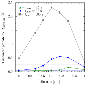
Figure E: Flow-dependent sperm-egg encounter probability for different exposure times $t_{\text{max}}$. Encounter probabilities $P_{\text{sperm:egg}}(\alpha)$ as function of external shear rate $\alpha$ for three values of sperm-egg exposure time $t_{\text{max}}$ obtained from simulations with co-rotation. (symbols according to legend, mean $\pm$ SD; flow-less results $P_{\text{sperm:egg}}(\alpha=0\leavevmode\nobreak\ \text{s}^{-1})$ displayed by dashed horizontal lines in respective color). Parameters taken for A. punctuala, see Table A, except boundary radius $r_{\text{max}}=15\leavevmode\nobreak\$mm for numerical efficiency.

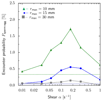
Figure F: Flow-dependent sperm-egg encounter probability for different egg densities $\rho_{\text{egg}}$. Analogous to Fig E, yet for three different values of boundary radius $r_{\text{max}}$, corresponding to three different egg densities $\rho_{\text{egg}}$ according to $\rho_{\text{egg}}=\left(4\pi r_{\text{max}}^{3}/3\right)^{-1}$. (For all three curves $t_{\text{max}}=90\leavevmode\nobreak\$s, thus blue curve identical to blue curve in Fig E.)

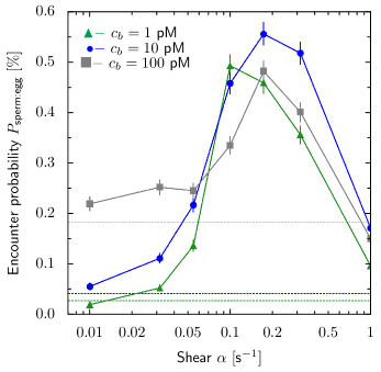
Figure G: Flow-dependent sperm-egg encounter probability for different thresholds of sensory adaption $c_{b}$. Analogous to Fig E, yet for three different values of threshold $c_{b}$. (For all three curves $t_{\text{max}}=90\leavevmode\nobreak\$s and $r_{\text{max}}=15$ mm, thus blue curve identical to blue curve in Fig E.)

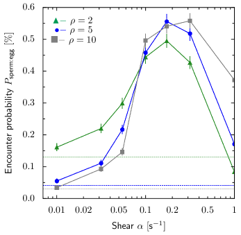
Figure H: Flow-dependent sperm-egg encounter probability for different gain factors $\rho$. Analogous to Fig E, yet for three different values of gain factor $\rho$. (For all three curves $t_{\text{max}}=90\leavevmode\nobreak\$s and $r_{\text{max}}=15$ mm, thus blue curve identical to blue curve in Fig E.)

Table B: Relative amplitude of optimum in sperm-egg encounter probability. Ratios of encounter probability $P_{\text{sperm:egg}}(\alpha=\alpha^{*})$ at optimal shear rate $\alpha^{*}$ normalized by encounter probability $P_{\text{sperm:egg}}(\alpha=0)$ in the absence of flow for parameter study displayed in Fig E, Fig F, Fig G, and Fig H.

Parameter	$P_{\text{sperm:egg}}(\alpha^{*})/P_{\text{sperm:egg}}(\alpha=0)$
Sperm-egg exposure time:
$t_{\text{max}}=$ 45 s, 90 s, 180 s	4.6	13.6	8.7
Boundary radius setting egg density:
$r_{\text{max}}=$ 10 mm, 15 mm, 30 mm	5.2	13.6	2.3
Threshold of sensory adaptation:
$c_{b}=$ 1 pM, 10 pM, 100 pM	18.3	13.6	2.6
Chemotactic gain factor:
$\rho=$ 2, 5, 10	3.8	13.6	18.6

References

- 1. Fraenkel GS, Gunn DL. The Orientation of Animals. Dover Publ., New York; 1961.
- 2. Berg HC, Brown DA. Chemotaxis in Escherichia coli analysed by three-dimensional tracking. Nature. 1972;239:500–504.
- 3. Devreotes PN, Zigmond SH. Chemotaxis in Eukaryotic Cells: A Focus on Leukocytes and Dictyostelium. Ann Rev Cell Biol. 1988;4(1):649–686.
- 4. Alvarez L, Friedrich BM, Gompper G, Kaupp UB. The Computational Sperm Cell. Trends in Cell Biology. 2014;24(3):198–207. doi:10.1016/j.tcb.2013.10.004.
- 5. Eisenbach M, Giojalas LC. Sperm guidance in mammals — an unpaved road to the egg. Nat Rev Mol Cell Biol. 2006;7(4):276–285. doi:10.1038/nrm1893.
- 6. Miller RL. Sperm chemo-orientation in the metazoa. Biol Fertil. 1985;2:275–337.
- 7. Riffell JA, Krug PJ, Zimmer RK. The ecological and evolutionary consequences of sperm chemoattraction. Proc Natl Acad Sci USA. 2004;101(13):4501–4506. doi:10.1073/pnas.0304594101.
- 8. Corkidi G, Taboada B, Wood CD, Guerrero A, Darszon A. Tracking sperm in three-dimensions. Biochem Biophys Res Commun. 2008;373(1):125–129. doi:10.1016/j.bbrc.2008.05.189.
- 9. Kaupp UB. 100 years of sperm chemotaxis. J Gen Physiol. 2012;140(6):583–586. doi:10.1085/jgp.201210902.
- 10. Serrão EA, Pearson G, Kautsky L, Brawley SH. Successful external fertilization in turbulent environments. Proc Natl Acad Sci USA. 1996;93(11):5286–5290. doi:10.1073/pnas.93.11.5286.
- 11. Gordon R, Brawley SH. Effects of water motion on propagule release from algae with complex life histories. Mar Bio. 2004;145(1):21–29. doi:10.1007/s00227-004-1305-y.
- 12. Levitan DR. The Importance of Sperm Limitation to the Evolution of Egg Size in Marine Invertebrates. Am Nat. 1993;141(4):517–536. doi:10.1086/285489.
- 13. Crenshaw HC. A New Look at Locomotion in Microorganisms: Rotating and Translating. Integr Comp Biol. 1996;36(6):608–618. doi:10.1093/icb/36.6.608.
- 14. Friedrich BM, Jülicher F. Chemotaxis of sperm cells. Proc Natl Acad Sci USA. 2007;104(33):13256–13261. doi:10.1073/pnas.0703530104.
- 15. Jikeli JF, Alvarez L, Friedrich BM, Wilson LG, Pascal R, Colin R, et al. Sperm Navigation along Helical Paths in 3D Chemoattractant Landscapes. Nat Commun. 2015;6:7985. doi:10.1038/ncomms8985.
- 16. Kashikar ND, Alvarez L, Seifert R, Gregor I, Jäckle O, Beyermann M, et al. Temporal Sampling, Resetting, and Adaptation Orchestrate Gradient Sensing in Sperm. J Cell Biol. 2012;198(6):1075–1091. doi:10.1083/jcb.201204024.
- 17. Kromer JA, Märcker S, Lange S, Baier C, Friedrich BM. Decision making improves sperm chemotaxis in the presence of noise. PLoS Comput Biol. 2018;14(4):e1006109. doi:10.1371/journal.pcbi.1006109.
- 18. Eisenbach M. Sperm chemotaxis. Rev Reprod. 1999;4(1):56–66. doi:10.1530/revreprod/4.1.56.
- 19. Riffell JA, Zimmer RK. Sex and flow: the consequences of fluid shear for sperm–egg interactions. J Exp Biol. 2007;210(20):3644–3660. doi:10.1242/jeb.008516.
- 20. Zimmer RK, Riffell JA. Sperm Chemotaxis, Fluid Shear, and the Evolution of Sexual Reproduction. Proc Natl Acad Sci USA. 2011;108(32):13200–13205. doi:10.1073/pnas.1018666108.
- 21. Taylor JR, Stocker R. Trade-Offs of Chemotactic Foraging in Turbulent Water. Science. 2012;338(6107):675–679. doi:10.1126/science.1219417.
- 22. Crimaldi JP, Zimmer RK. The Physics of Broadcast Spawning in Benthic Invertebrates. Annu Rev Mar Sci. 2014;6:141–165. doi:10.1146/annurev-marine-010213-135119.
- 23. Rusconi R, Guasto JS, Stocker R. Bacterial transport suppressed by fluid shear. Nat Phys. 2014;10(3):212–217. doi:10.1038/nphys2883.
- 24. Lazier JRN, Mann KH. Turbulence and the Diffusive Layers around Small Organisms. Deep-Sea Res I. 1989;36(11):1721–1733. doi:10.1016/0198-0149(89)90068-X.
- 25. Mead KS, Denny MW. The Effects of Hydrodynamic Shear Stress on Fertilization and Early Development of the Purple Sea Urchin Strongylocentrotus purpuratus. Biol Bull. 1995;188(1):46–56. doi:10.2307/1542066.
- 26. Jumars PA, Trowbridge JH, Boss E, Karp-Boss L. Turbulence-Plankton Interactions: A New Cartoon. Mar Ecol. 2009;30(2):133–150. doi:10.1111/j.1439-0485.2009.00288.x.
- 27. Sreenivasan KR. Turbulent mixing: A perspective. Proc Natl Acad Sci USA. 2019;116(37):18175–18183. doi:10.1073/pnas.1800463115.
- 28. Denny, Shibata MF. Consequences of Surf-Zone Turbulence for Settlement and External Fertilization. Am Nat. 1989;134:859–889.
- 29. Bell AF, Crimaldi JP. Effect of Steady and Unsteady Flow on Chemoattractant Plume Formation and Sperm Taxis. J Marine Syst. 2015;148:236–248. doi:10.1016/j.jmarsys.2015.03.008.
- 30. Jeffery GB. The Motion of Ellipsoidal Particles Immersed in a Viscous Fluid. Proc R Soc Lon A. 1922;102(715):161–179. doi:10.1098/rspa.1922.0078.
- 31. Pedley TJ, Kessler JO. Hydrodynamic Phenomena in Suspensions of Swimming Microorganisms. Annu Rev Fluid Mech. 1992;24(1):313–358. doi:10.1146/annurev.fl.24.010192.001525.
- 32. Hein AM, Martin BT. Information limitation and the dynamics of coupled ecological systems. Nat Ecol Evol. 2020;4(1):82–90. doi:10.1038/s41559-019-1008-x.
- 33. Friedrich BM. Search along persistent random walks. Phys Biol. 2008;5(2):026007. doi:10.1088/1478-3975/5/2/026007.
- 34. Vogel H, Czihak G, Chang P, Wolf W. Fertilization kinetics of sea urchin eggs. Math Biosci. 1982;58(2):189–216. doi:10.1016/0025-5564(82)90073-6.
- 35. Levitan DR, Sewell MA, Chia FS. Kinetics of Fertilization in the Sea Urchin Strongylocentrotus franciscanus: Interaction of Gamete Dilution, Age, and Contact Time. Biol Bull. 1991;181(3):371–378. doi:10.2307/1542357.
- 36. Styan CA. Polyspermy, Egg Size, and the Fertilization Kinetics of Free-Spawning Marine Invertebrates. Am Nat. 1998;152(2):290–297. doi:10.1086/286168.
- 37. Millar RB, Anderson MJ. The kinetics of monospermic and polyspermic fertilization in free-spawning marine invertebrates. J Theor Biol. 2003;224(1):79–85. doi:10.1016/S0022-5193(03)00145-0.
- 38. Gaylord B. Hydrodynamic Context for Considering Turbulence Impacts on External Fertilization. Biol Bull. 2008;214(3):315–318. doi:10.2307/25470672.
- 39. Denny MW, Nelson EK, Mead KS. Revised Estimates of the Effects of Turbulence on Fertilization in the Purple Sea Urchin, Strongylocentrotus purpuratus. Biol Bull. 2002;203(3):275–277. doi:10.2307/1543570.
- 40. Kolmogorov A. The Local Structure of Turbulence in Incompressible Viscous Fluid for Very Large Reynolds’ Numbers. Akademiia Nauk SSSR Doklady. 1941;30:301–305.
- 41. Kolmogorov AN. A refinement of previous hypotheses concerning the local structure of turbulence in a viscous incompressible fluid at high Reynolds number. J Fluid Mech. 1962;13(1):82–85. doi:10.1017/S0022112062000518.
- 42. Luchsinger RH, Bergersen B, Mitchell JG. Bacterial Swimming Strategies and Turbulence. Biophys J. 1999;77(5):2377–2386. doi:10.1016/S0006-3495(99)77075-X.
- 43. Locsei JT, Pedley TJ. Run and Tumble Chemotaxis in a Shear Flow: The Effect of Temporal Comparisons, Persistence, Rotational Diffusion, and Cell Shape. Bull Math Biol. 2009;71(5):1089–1116. doi:10.1007/s11538-009-9395-9.
- 44. Stocker R. Marine Microbes See a Sea of Gradients. Science. 2012;338(6107):628–633. doi:10.1126/science.1208929.
- 45. Kiørboe T, Saiz T. Planktivorous feeding in calm and turbulent environments, with emphasis on copepods. Mar Ecol Prog Ser. 1995;122:135–145. doi:10.3354/meps122135.
- 46. Breier RE, Lalescu CC, Waas D, Wilczek M, Mazza MG. Emergence of phytoplankton patchiness at small scales in mild turbulence. Proc Natl Acad Sci USA. 2018;115(48):12112–12117. doi:10.1073/pnas.1808711115.
- 47. Lombard F, Koski M, Kiørboe T. Copepods use chemical trails to find sinking marine snow aggregates. Limnol Oceanogr. 2013;58(1):185–192. doi:10.4319/lo.2013.58.1.0185.
- 48. Brumley DR, Carrara F, Hein AM, Hagstrom GI, Levin SA, Stocker R. Cutting Through the Noise: Bacterial Chemotaxis in Marine Microenvironments. Front Mar Sci. 2020;7. doi:10.3389/fmars.2020.00527.
- 49. Suarez SS, Pacey AA. Sperm transport in the female reproductive tract. Hum Reprod Update. 2006;12(1):23–37. doi:10.1093/humupd/dmi047.
- 50. Gaffney EA, Gadêlha H, Smith DJ, Blake JR, Kirkman-Brown JC. Mammalian Sperm Motility: Observation and Theory. Annu Rev Fluid Mech. 2011;43(1):501–528. doi:10.1146/annurev-fluid-121108-145442.
- 51. Miki K, Clapham D. Rheotaxis Guides Mammalian Sperm. Current Biology. 2013;23(6):443–452. doi:10.1016/j.cub.2013.02.007.
- 52. Kantsler V, Dunkel J, Blayney M, Goldstein RE. Rheotaxis facilitates upstream navigation of mammalian sperm cells. eLife. 2014;3:e02403. doi:10.7554/eLife.02403.
- 53. Marcos H, Fu HC, Powers TR, Stocker R. Bacterial rheotaxis. Proc Natl Acad Sci USA. 2012;109(13):4780–4785. doi:10.1073/pnas.1120955109.
- 54. Hein AM, Carrara F, Brumley DR, Stocker R, Levin SA. Natural search algorithms as a bridge between organisms, evolution, and ecology. Proc Natl Acad Sci USA. 2016;113(34):9413–9420. doi:10.1073/pnas.1606195113.
- 55. Lancia F, Yamamoto T, Ryabchun A, Yamaguchi T, Sano M, Katsonis N. Reorientation behavior in the helical motility of light-responsive spiral droplets. Nat Commun. 2019;10(1):1–8. doi:10.1038/s41467-019-13201-6.
- 56. Xu H, Medina-Sánchez M, Magdanz V, Schwarz L, Hebenstreit F, Schmidt OG. Sperm-Hybrid Micromotor for Targeted Drug Delivery. ACS Nano. 2018;12(1):327–337. doi:10.1021/acsnano.7b06398.
- 57. Klindt GS, Ruloff C, Wagner C, Friedrich BM. Load Response of the Flagellar Beat. Phys Rev Lett. 2016;117(25):258101. doi:10.1103/PhysRevLett.117.258101.
- 58. Mikulencak DR, Morris JF. Stationary Shear Flow around Fixed and Free Bodies at Finite Reynolds Number. J Fluid Mech. 2004;520:215–242. doi:10.1017/S0022112004001648.
- 59. Friedrich BM, Jülicher F. Steering Chiral Swimmers along Noisy Helical Paths. Phys Rev Lett. 2009;103(6):068102. doi:10.1103/PhysRevLett.103.068102.
- 60. Rodrigues O. Des lois géométriques qui régissent les déplacements d’un système solide dans l’espace, et de la variation des coordonnées provenant de ces déplacements considérés indépendamment des causes qui peuvent les produire. J Math Pures Appl. 1840; p. 380–440.
- 61. Frankel NA, Acrivos A. Heat and Mass Transfer from Small Spheres and Cylinders Freely Suspended in Shear Flow. Phys Fluids. 1968;11(9):1913–1918. doi:10.1063/1.1692218.
- 62. Elrick DE. Source Functions for Diffusion in Uniform Shear Flow. Aust J Phys. 1962;15(3):283–288. doi:10.1071/ph620283.
- 63. Zöttl A, Stark H. Nonlinear Dynamics of a Microswimmer in Poiseuille Flow. Phys Rev Lett. 2012;108(21):218104. doi:10.1103/PhysRevLett.108.218104.
- 64. Zöttl A, Stark H. Periodic and Quasiperiodic Motion of an Elongated Microswimmer in Poiseuille Flow. Eur Phys J E. 2013;36(1):4. doi:10.1140/epje/i2013-13004-5.
- 65. Słomka J, Alcolombri U, Secchi E, Stocker R, Fernandez VI. Encounter rates between bacteria and small sinking particles. New J Phys. 2020;22(4):043016. doi:10.1088/1367-2630/ab73c9.
- 66. Mead KS. Sex in the surf zone: the effect of hydrodynamic shear stress on the fertilization and early development of free-spawning invertebrates [Ph.D. thesis]. Stanford University; 1996. Available from: https://dennylab.stanford.edu/publications/sex-surf-zone-effect-hydrodynamic-shear-stress-fertilization-and-early-development-free.
- 67. Alvarez L, Dai L, Friedrich BM, Kashikar ND, Gregor I, Pascal R, et al. The rate of change in Ca2+ concentration controls sperm chemotaxis. J Cell Biol. 2012;196(5):653–663. doi:10.1083/jcb.201106096.
- 68. Horst Gvd, Bennett M, Bishop JDD. CASA in invertebrates. Reproduction Fertility and Development. 2018;30(6):907–918. doi:10.1071/RD17470.
- 69. Friedrich BM. Chemotaxis of Sperm cells [Ph.D. thesis]. TU Dresden; 2008. Available from: https://cfaed.tu-dresden.de/files/user/bfriedrich/papers/friedrich_chemotaxis_sperm_cells_phd_2009.pdf.
- 70. Pichlo M, Bungert-Plümke S, Weyand I, Seifert R, Bönigk W, Strünker T, et al. High density and ligand affinity confer ultrasensitive signal detection by a guanylyl cyclase chemoreceptor. J Cell Biol. 2014;206(4):541–557. doi:10.1083/jcb.201402027.
- 71. Hatakeyama N, Kambe T. Statistical Laws of Random Strained Vortices in Turbulence. Phys Rev Lett. 1997;79(7):1257–1260. doi:10.1103/PhysRevLett.79.1257.
- 72. Webster DR, Young DL. A Laboratory Realization of the Burgers’ Vortex Cartoon of Turbulence-Plankton Interactions. Limnol Oceanogr: Methods. 2015;13(2):92–102. doi:10.1002/lom3.10010.
- 73. Berg HC, Purcell EM. Physics of chemoreception. Biophysical Journal. 1977;20(2):193–219. doi:10.1016/S0006-3495(77)85544-6.
- 74. Kromer JA, de la Cruz N, Friedrich BM. Chemokinetic Scattering, Trapping, and Avoidance of Active Brownian Particles. Phys Rev Lett. 2020;124(11):118101. doi:10.1103/PhysRevLett.124.118101.