Detecting Incorrect Behavior of Cloud Databases as an Outsider

Abstract

Cloud DBs offer strong properties, including serializability, sometimes called the gold standard database correctness property. But cloud DBs are complicated black boxes, running in a different administrative domain from their clients; thus, clients might like to know whether the DBs are meeting their contract. A core difficulty is that the underlying problem here, namely verifying serializability, is NP-complete [91]. Nevertheless, we hypothesize that on real-world workloads, verifying serializability is tractable, and we treat the question as a systems problem, for the first time. We build cobra, which tames the underlying search problem by blending a new encoding of the problem, hardware acceleration, and a careful choice of a suitable SMT solver. cobra also introduces a technique to address the challenge of garbage collection in this context. cobra improves over natural baselines by at least 10$\times$ in the problem size it can handle, while imposing modest overhead on clients.

1 Introduction and motivation

A new class of cloud databases has emerged, including products from Google [51, 14, 13], Amazon [110, 2], Microsoft Azure [3], as well as their “cloud-native” open source alternatives [5, 24, 9, 10]. Compared to earlier generations of NoSQL databases (such as Facebook Cassandra, Google Bigtable, and Amazon S3), members of the new class offer the same scalability, availability, replication, and geodistribution but in addition support a powerful programming construct: strong ACID transactions. By “strong”, we mean that the promised isolation contract is serializability [91, 40]: all transactions appear to execute in a single, sequential order.

Serializability is the “gold standard” isolation level [34], and the one that many applications and programmers implicitly assume (in the sense that their code is incorrect if the database provides a weaker contract) [112]. As the essential correctness contract, serializability is the visible part of the entire iceberg (the cloud). This has to do with how the cloud database is used [15, 18]: a user (developer or administrator) deploys, for example, web servers as database clients. And, based on whether the observed behaviors from clients are serializable, the user can deduce whether the cloud database has operated as expected. In particular, if the database has satisfied serializability throughout one’s observation, then the user knows that the database maintains basic integrity: each value read derives from a valid write. It also implies that the database has survived failures (if any) during this period.

A user can legitimately wonder whether cloud databases in fact provide the promised contract. For one thing, users have no visibility into a cloud database’s internals. Any internal corruption—as could happen from misconfiguration, misoperation, compromise, or adversarial control at any layer of the execution stack—can result in serializability violation. And for another, one need not adopt a paranoid stance (“the cloud as malicious adversary”) to acknowledge that it is difficult, as a technical matter, to provide serializability and geo-distribution and geo-replication and high performance under various failures [27, 120, 60]. Doing so usually involves a consensus protocol that interacts with an atomic commit protocol [51, 78, 85]—a complex, and hence potentially bug-prone, combination.

As serializability is a critical guarantee, verifying that the database is serializable is an important issue. Indeed, existing works [108, 102, 90, 115, 68, 117, 45] can verify serializability and/or other consistency anomalies. However, these works share a limitation: they require “inside information”—(parts of) the internal schedules of the database. Crucially, such internal schedules are invisible to the clients of cloud databases. This leads to our question: how can clients verify the serializability of a cloud database without inside information?

On the one hand, this question has long been known to be intractable: Papadimitriou proved its NP-completeness 40 years ago [91]. On the other hand, one of the remarkable aspects in the field of formal verification has been the use of heuristics to “solve” problems whose general form is intractable; recent examples include [70, 69, 59]. This owes to major advances in solvers (advanced SAT and SMT solvers) [89, 65, 81, 107, 42, 55, 35, 48], coupled with an explosion of computing power. Thus, our guiding intuition is that it ought to be possible to verify serializability (without inside information) in many real-world cases.

And so, we are motivated to treat the italicized question as a systems problem, for the first time. Compared to prior works [99, 115, 102, 84] (§7), our underlying technical problem is different and computationally harder, which consists of (a) positing an unmodifiable and black-box database, (b) retaining the database’s throughput and latency, and (c) checking serializability, rather than a weaker property.

This paper describes a system called cobra. cobra comprises a third-party database (which cobra does not modify); a set of (legacy) database clients (which cobra modifies to link to a library); one or more history collectors that record requests and responses to the database; and a verifier. The history collectors periodically send history fragments to the verifier, which has to determine whether the observed history is serializable. The deployer of cobra (also, the user of the cloud database) defines the trust domain which encompasses database clients, collectors, and the verifier; while the database is untrusted. Section 2 further details the setup. cobra’s verifier solves two main problems, outlined below.

1. Efficient witness search (§3). One can check serializability by searching for an acyclic graph whose vertices are transactions and whose edges obey certain constraints; a constraint specifies that exactly one of two edges must be in the searched-for graph. From this description, one suspects that a SAT/SMT solver [55, 23, 106, 36] would be useful. But complications arise. To begin with, encoding acyclicity in a SAT instance brings overhead [61, 62, 74] (we see this too; §6.1). Instead, cobra uses a recent SMT solver, MonoSAT [38], that is well-suited to checking graph properties (§3.4). However, even MonoSAT alone is too inefficient (§6.1).

To address this issue, cobra reduces the search problem size. First, cobra introduces a new encoding that exploits common patterns in real workloads, such as read-modify-write transactions, to efficiently infer ordering relationships from a history (§3.1–§3.2). (We prove that cobra’s encoding is a valid reduction in Appendix A.) Second, cobra uses parallel hardware (our implementation uses GPUs; §5) to compute all-paths reachability over the known graph edges; then, cobra is able to efficiently resolve some of the constraints, by testing whether a candidate edge would generate a cycle with an existing path.

2. Garbage collection and scaling (§4). cobra’s verifier works in rounds. From round-to-round, however, the verifier must trim history, otherwise verification would become too costly. The challenge is that the verifier seemingly needs to retain all history, because serializability does not respect real-time ordering, so future transactions can read from values that (in a real-time view) have been overwritten (§4.1). To solve this problem, clients issue periodic fence transactions (§4.2). The fences impose coarse-grained synchronization, creating a window from which future reads, if they are to be serializable, are permitted to read. This allows the verifier to discard transactions prior to the window.

We implement cobra (§5) and find (§6) that, compared to our baselines, cobra delivers at least a 10$\times$ improvement in the problem size it can handle (verifying a history of 10k transactions in 14 seconds), while imposing minor throughput and latency overhead on clients. End-to-end, on an ongoing basis, cobra can sustainably verify 1k–2.5k txn/sec on the workloads that we experiment with.

cobra’s main limitations are: First, given the underlying problem is NP-complete, theoretically there is no guarantee that cobra can terminate (though all our experiments finish in reasonable time, §6). Second, range queries are not natively supported by cobra; programmers need to add extra meta-data in database schemas to help check serializability on range queries.

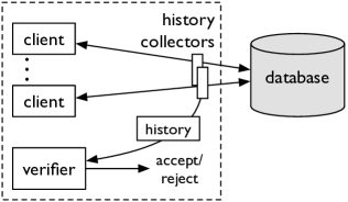
Figure 1: Architecture of cobra. The trust domain is framed by dashed lines.

2 Overview and background

Figure 1 depicts cobra’s high-level architecture. Clients issue requests to a database and receive results. The database is untrusted: the results can be arbitrary.

Each client request is one of five operations: start, commit, abort (which refer to transactions), and read and write (which refer to keys). Each client is single-threaded: it waits to receive the result of the current request before issuing the next request.

A set of history collectors sit between clients and the database, and capture the requests that clients issue and the (possibly wrong) results delivered by the database. This capture is a fragment of a history. A history is a set of operations; it is the union of the fragments from all collectors.

A verifier retrieves history fragments from collectors and verifies whether the history is serializable; we defined this term loosely in the introduction and will make it more precise below (§2.1). Verification proceeds in rounds; each round consists of a witness search, the input to which is logically the output of the previous round and new history fragments. Clients, history collectors, and the verifier are trusted.

cobra’s architecture is relevant in real-world scenarios. As an example, an enterprise web application uses a cloud database for stability, performance, and fault-tolerance. The end-users of this application are geo-distributed employees of the enterprise. To avoid confusion, note that the employees are users of the application, and the clients here are the web application servers, as clients of the database.

Database clients (the application) run on the enterprise’s hardware (“on-premises”) while the database runs on an untrusted cloud provider. The verifier also runs on-premises. In this setup, collectors can be middleboxes situated at the edge of the enterprise and can thereby capture the requests/responses between the clients and the database in the cloud.

The rest of this section defines the core problem more precisely and gives the starting point for cobra’s solution. Section 3 describes cobra’s techniques for a single instance of the problem while Section 4 describes the techniques needed to stitch rounds together.

2.1 Preliminaries

First, assume that each value written to the database is unique; thus, from the history, any read (in a transaction) can be associated with the unique transaction that issued the corresponding write. cobra discharges this assumption with logic in the cobra client library (§5).

A history is a set of read and write operations, each of which is associated with a transaction. Each read operation must read from a particular write operation in the history. A history is serializable if it matches a serial schedule [91]. A schedule is a total order of all operations in the history. A history and schedule match each other if executing the operations following the schedule on a set of single-copy data produces the same read results as the history. (The write operations are assumed to have empty returns so are irrelevant in matching a history and a schedule.) A serial schedule means that the schedule does not have overlapping transactions. In addition to a serializable history, we also say a schedule is serializable if the schedule is equivalent to a serial schedule—executing the two schedules generates the same read results and leaves the data in the same final state.

A schedule implies an ordering for every pair of conflicting operations; two operations conflict if they are from different transactions and at least one is write. These orderings (all of them) form a set of dependencies among the transactions. For example, if an operation of a transaction $T_{1}$ writes a key, and later in the schedule, an operation of transaction $T_{2}$ writes the same key, the dependency set contains a dependency denoted as $T_{1}\rightarrow T_{2}$.

From a schedule and its dependency set, one can construct a precedence graph that has a vertex for every transaction in the schedule and a directed edge for every dependency implied by the schedule. An important fact is that if the precedence graph is acyclic, a serial schedule that is equivalent to the original schedule can be derived, by topologically sorting the precedence graph.

2.2 Verification problem statement

Based on the immediately preceding fact, the question of whether a history is serializable can be converted to whether the history matches a schedule whose precedence graph is acyclic. So, the core problem is to identify such a precedence graph, or assert that none exists.

Note that this question would be straightforward if the database revealed its actual schedule (thus ruling out any other possible schedule): one could construct that schedule’s precedence graph, and test it for acyclicity. Indeed, this is the problem of testing conflict-serializability [113]. Our problem, however, is testing view-serializability [116]. In our context, where the database is a black box (§1, §2), we have to (implicitly) find schedules that match the history, and test those schedules’ precedence graphs for acyclicity. Intuitively, we will conduct this search by first listing all edges that must exist—for example, a transaction reads from another’s write—and then consider the edges between every other pair of conflicting transactions (operations) as possibilities.

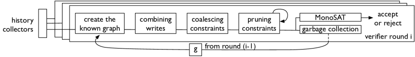
Figure 2: The verifier’s process, within a round and across rounds.

2.3 Starting point: Intuition and brute force

This section describes a brute-force solution, which serves as the starting point for cobra and gives intuition. The approach relies on a data structure called a polygraph [91], which captures all possible precedence graphs when some of the dependencies are unknown.

In a polygraph, vertices ($V$) are transactions and edges ($E$) are read-dependencies. A set $C$, which we call constraints, indicates possible (but unknown) dependencies. Here is an example polygraph:

It has three vertices $V=\{T_{1},T_{2},T_{3}\}$, one known edge $E=\{(T_{1},T_{3})\}$ from $W_{1}(x)\xrightarrow[]{\text{wr(x)}}R_{3}(x)$, and one constraint $\langle\,(T_{3},\,T_{2}),\ (T_{2},\,T_{1})\,\rangle$ which is shown as two dashed arrows connected by an arc. This constraint captures the fact that $T_{3}$ cannot happen in between $T_{1}$ and $T_{2}$, because $T_{3}$ reads $x$ from $T_{1}$; and $T_{2}$ which writes $x$ either happens before $T_{1}$ or after $T_{3}$. But it is unknown which option is the truth.

Formally, a polygraph $P=(V,\ E,\ C)$ is a directed graph $(V,\ E)$ together with a set of bipaths, $C$; that is, pairs of edges—not necessarily in $E$—of the form $\langle(v,\,u),\ (u,\,w)\rangle$ such that $(w,\,v)\in E$. A bipath of that form can be read as “either $u$ happened after $v$, or else $u$ happened before $w$”.

Now, define the polygraph $(V,\,E,\,C)$ associated with a history, as follows [113]:

• $V$ are all committed transactions in the history

• $E=\{(T_{i},\,T_{j})\,|\,T_{j}\textrm{ reads from }T_{i}\}$; that is, $T_{i}\xrightarrow[]{\text{wr(x)}}T_{j}$, for some $x$.

• $C=\{\langle\,(T_{j},\,T_{k}),\ (T_{k},\,T_{i})\,\rangle\mid(T_{i}\xrightarrow[]{\text{wr(x)}}T_{j})\,\land\,\\ \hskip 30.00005pt(T_{k}\textrm{\ writes to $x$})\land T_{k}\neq T_{i}\land T_{k}\neq T_{j}\}$.

The edges in $E$ capture a class of dependencies (§2.1) that are evident from the history, known as WR dependencies (a transaction writes a key, and another transaction reads the value written to that key). The third bullet describes how uncertainty is encoded into constraints. Specifically, for each WR dependency in the history, all other transactions that write the same key either happen before the given write or else after the given read.

A precedence graph is called compatible with a polygraph if: the precedence graph has the same nodes and known edges in the polygraph, and the precedence graph chooses one edge out of each constraint. Formally, a precedence graph $(V^{\prime},E^{\prime})$ is compatible with a polygraph $(V,\,E,\,C)$ if: $V=V^{\prime}$, $E\subseteq E^{\prime}$, and $\forall\langle e_{1},\,e_{2}\rangle\in C,\ (e_{1}\in E^{\prime}\land e_{2}\notin E^{\prime})\lor(e_{1}\notin E^{\prime}\land e_{2}\in E^{\prime})$.

A crucial fact is: there exists an acyclic precedence graph that is compatible with the polygraph associated to a history if and only if that history is serializable [91, 113]. This yields a brute-force approach for verifying serializability: first, construct a polygraph from a history; second, search for a compatible precedence graph that is acyclic. However, not only does this approach need to consider $|C|$ binary choices ($2^{|C|}$ possibilities) but also $|C|$ is massive: it is a sum of quadratic terms, specifically $\sum_{k\in\mathcal{K}}p_{\textit{k}}\cdot(q_{\textit{k}}-1)$, where $\mathcal{K}$ is the set of keys in the history, and each $p_{k},q_{k}$ are (respectively) the number of reads and writes of key $k$.

3 Verifying serializability in cobra

Figure 2 depicts the verifier and the major components of verification. This section covers one round of verification. As a simplification, assume that the round runs in a vacuum; Section 4 discusses how rounds are linked.

cobra uses an SMT solver geared to graph properties, specifically MonoSAT [38] (§3.4). Yet, despite MonoSAT’s power, encoding the problem as in Section 2.3 would generate too much work for it (§6.1).

cobra refines that encoding in several ways. It introduces write combining (§3.1) and coalescing (§3.2). These techniques are motivated by common patterns in workloads, and efficiently extract restrictions (on the search space) that are available in the history. cobra’s verifier also does its own inference (§3.3), prior to invoking the solver. This is motivated by observing that (a) having all-pairs reachability information (in the “known edges”) yields quick resolution of many constraints, and (b) computing that information is amenable to acceleration on parallel hardware such as GPUs (the computation is iterated matrix multiplication; §5).

Figure 3 depicts the algorithm that constructs cobra’s encoding and shows how the techniques combine. Note that cobra relies on a generalized notion of constraints. Whereas previously a constraint was a pair of edges, now a constraint is a pair of sets of edges. Meeting a constraint $\langle A,B\rangle$ means including all edges in $A$ and excluding all in $B$, or vice versa. More formally, we say that a precedence graph $(V^{\prime},E^{\prime})$ is compatible with a known graph $G=(V,E)$ and generalized constraints $C$ if: $V=V^{\prime}$, $E\subseteq E^{\prime}$, and $\forall\langle A,\,B\rangle\in C,(A\subseteq E^{\prime}\land B\cap E^{\prime}=\emptyset)\lor(A\cap E^{\prime}=\emptyset\land B\subseteq E^{\prime})$.

We prove the validity of cobra’s encoding in Appendix A. Specifically we prove that there exists an acyclic graph that is compatible with the constraints constructed by cobra on a given history if and only if the history is serializable.

 

1:procedure ConstructEncoding(history)

2:   $\textit{g},\,\textit{readfrom},\,\textit{wwpairs}\leftarrow\mbox{{CreateKnownGraph}}(\textit{history})$

3:   $\textit{con}\leftarrow\mbox{{GenConstraints}}(\textit{g},\,\textit{readfrom},\,\textit{wwpairs})$

4:   $\textit{con},\,\textit{g}\leftarrow\mbox{{Prune}}(\textit{con},\,\textit{g})$ // §3.3, executed one or more times

5:   return con, g

6:

7:procedure CreateKnownGraph(history)

8:   $\textit{g}\leftarrow$ empty graph                              // the konwn graph

9:   $\textit{wwpairs}\leftarrow$ map $\{\langle\textrm{Key},\textrm{Tx}\rangle\to\textrm{Tx}\}$      // consecutive writes

10:   // map from a write Tx to a set of read Txs that read this write

11:   $\textit{readfrom}\leftarrow$ map $\{\langle\textrm{Key},\textrm{Tx}\rangle\to\textrm{Set}\langle\textrm{Tx}\rangle\}$

12:   for transaction tx in history:

13:      $\textit{g}.\textrm{Nodes}\mathrel{+}=\textit{tx}$

14:      for read operation rop in tx :

15:         $\textit{g}.\textrm{Edges}\mathrel{+}=(\textit{rop}.\textrm{read\_from\_tx},\ \textit{tx})$     // add wr-edge

16:         $\textit{readfrom}[\langle\textit{rop}.\textrm{key},\,\textit{rop}.\textrm{read\_from\_tx}\rangle]\mathrel{+}=\textit{tx}$       

17:      

18:      // detect RMW (read-modify-write) transactions

19:      for all Keys key that are both read and written by tx:

20:         rop $\leftarrow$ the operation in tx that reads key

21:         if $\textit{wwpairs}[\langle\textit{key},\,\textit{rop}.\textrm{read\_from\_tx}\rangle]\neq\textit{null}$:

22:            reject     // two successive writes, not serializable          

23:         $\textit{wwpairs}[\langle\textit{key},\,\textit{rop}.\textrm{read\_from\_tx}\rangle]\leftarrow\textit{tx}$          

24:   

25:   return $\textit{g},\ \textit{readfrom},\ \textit{wwpairs}$

26:

27:procedure GenConstraints($\textit{g},\,\textit{readfrom},\,\textit{wwpairs}$)

28:   // each key maps to set of chains; each chain is an ordered list

29:   $\textit{chains}\leftarrow$ empty map {$\textrm{Key}\to\textrm{Set}\langle\textrm{List}\rangle$}

30:   for transaction tx in g :

31:      for write wrop in tx :

32:         chains[wrop.key] $\mathrel{+}=$ [ tx ]     // one-element list          

33:   

34:   $\mbox{{CombineWrites}}(\textit{chains},\,\textit{wwpairs})$      // §3.1

35:   $\mbox{{InferRWEdges}}(\textit{chains},\,\textit{readfrom},\,\textit{g})$ // infer anti-dependency

36:   

37:   $\textit{con}\leftarrow$ empty set

38:   for $\langle\textit{key},\textit{chainset}\rangle$ in chains:

39:      for every pair $\{\textit{chain}_{i},\,\textit{chain}_{j}\}$ in chainset:

40:         $\textit{con}\mathrel{+}=\mbox{{Coalesce}}(\textit{chain}_{i},\,\textit{chain}_{j},\,\textit{key},\,\textit{readfrom})$ // §3.2          

41:   

42:   return con

43:procedure CombineWrites($\textit{chains},\,\textit{wwpairs}$)

44:   for $\langle\textit{key},\,\textit{tx}_{1},\,\textit{tx}_{2}\rangle$ in wwpairs :

45:      // By construction of wwpairs, $\textit{tx}_{1}$ is the write immediately

46:      // preceding $\textit{tx}_{2}$ on key. Thus, we can sequence all writes

47:      // prior to $\textit{tx}_{1}$ before all writes after $\textit{tx}_{2}$, as follows:

48:      $\textit{chain}_{1}\leftarrow$ the list in $\textit{chains}[\textit{key}]$ whose last elem is $\textit{tx}_{1}$

49:      $\textit{chain}_{2}\leftarrow$ the list in $\textit{chains}[\textit{key}]$ whose first elem is $\textit{tx}_{2}$

50:      $\textit{chains}[\textit{key}]\mathrel{\setminus}=\{\textit{chain}_{1},\,\textit{chain}_{2}\}$

51:      $\textit{chains}[\textit{key}]\mathrel{+}=\textrm{concat}(\textit{chain}_{1},\textit{chain}_{2})$    

52:

53:procedure InferRWEdges($\textit{chains},\,\textit{readfrom},\,\textit{g}$)

54:   for $\langle\textit{key},\textit{chainset}\rangle$ in chains:

55:      for chain in chainset:

56:         for $i$ in $[0,\,\textrm{length}(\textit{chain})-2]$:

57:            for rtx in $\textit{readfrom}[\langle\textit{key},\textit{chain}[i]\rangle]$:

58:               if ($\textit{rtx}\neq\textit{chain}[i\textrm{+}1]$): $\textit{g}.\textrm{Edges}\mathrel{+}=(\textit{rtx},\,\textit{chain}[i\textrm{+}1])$                               

59:

60:procedure Coalesce($\textit{chain}_{1},\,\textit{chain}_{2},\,\textit{key},\,\textit{readfrom}$)

61:   $\textit{edge\_set}_{1}\leftarrow\mbox{{GenChainToChainEdges}}(\textit{chain}_{1},\,\textit{chain}_{2},\,\textit{key},\,\textit{readfrom})$

62:   $\textit{edge\_set}_{2}\leftarrow\mbox{{GenChainToChainEdges}}(\textit{chain}_{2},\,\textit{chain}_{1},\,\textit{key},\,\textit{readfrom})$

63:   return $\langle\textit{edge\_set}_{1},\,\textit{edge\_set}_{2}\rangle$

64:

65:procedure GenChainToChainEdges($\textit{chain}_{i},\,\textit{chain}_{j},\,\textit{key},\,\textit{readfrom}$)

66:   if $\textit{readfrom}[\langle\textit{key},\,\textit{chain}_{i}.\textrm{tail}\rangle]=\emptyset$:

67:      $\textit{edge\_set}\leftarrow\{(\textit{chain}_{i}.\textrm{tail},\,\textit{chain}_{j}.\textrm{head})\}$

68:      return edge_set   

69:   

70:   $\textit{edge\_set}\leftarrow$ empty set

71:   for rtx in $\textit{readfrom}[\langle\textit{key},\,\textit{chain}_{i}.\textrm{tail}\rangle]$:

72:      $\textit{edge\_set}\mathrel{+}=(\textit{rtx},\,\textit{chain}_{j}.\textrm{head})$    

73:   return edge_set

74:

75:procedure Prune($\textit{con},\,\textit{g}$)

76:   // tr is the transitive closure (reachability of every two nodes) of g

77:   $\textit{tr}\leftarrow\mbox{{TransitiveClosure}}(\textit{g})$  // standard algorithm; see [52, Ch.25]

78:   for c =$\langle\textit{edge\_set}_{1},\,\textit{edge\_set}_{2}\rangle$ in con :

79:      if $\exists(\textit{tx}_{i},\,\textit{tx}_{j})\in\textit{edge\_set}_{1}\ s.t.\ \textit{tx}_{j}\rightsquigarrow\textit{tx}_{i}$ in tr:

80:         $\textit{g}.\textrm{Edges}\leftarrow\textit{g}.\textrm{Edges}\cup\textit{edge\_set}_{2}$

81:         $\textit{con}\mathrel{-}=\textit{c}$

82:      else if $\exists(\textit{tx}_{i},\,\textit{tx}_{j})\in\textit{edge\_set}_{2}\ s.t.\ \textit{tx}_{j}\rightsquigarrow\textit{tx}_{i}$ in tr:

83:         $\textit{g}.\textrm{Edges}\leftarrow\textit{g}.\textrm{Edges}\cup\textit{edge\_set}_{1}$

84:         $\textit{con}\mathrel{-}=\textit{c}$          

85:   return con, g

 

Figure 3: cobra’s procedure for converting a history into a constraint satisfaction problem (§3). After this procedure, cobra feeds the results (a graph of known edges $G$ and set of constraints $C$) to a constraint solver (§3.4), which searches for a graph that includes the known edges from $G$, meets the constraints in $C$, and is acyclic. We prove the algorithm’s validity in Appendix A.

3.1 Combining writes

cobra exploits the read-modify-write (RMW) pattern, in which a transaction reads a key and then writes the same key. The pattern is common in real-world scenarios, for example shopping: in one transaction, get the number of an item in stock, decrement, and write back the number. cobra uses RMWs to impose order on writes; this reduces the orderings that the verification procedure would otherwise have to consider. Here is an example:

There are four transactions, all operating on the same key. Two of the transactions are RMW, namely $R_{2},W_{2}$ and $R_{4},W_{4}$. On the left is the basic polygraph (§2.3); it has four constraints (each in a different color), which are derived from considering WR dependencies.

cobra, however, infers chains. A single chain comprises a sequence of transactions whose write operations are consecutive; in the figure, a chain is indicated by a shaded area. Notice that the only ordering possibilities exist at the granularity of chains (rather than individual writes); in the example, the two possibilities of course are $[W_{1},\,W_{2}]\to[W_{3},\,W_{4}]$ and $[W_{3},\,W_{4}]\to[W_{1},\,W_{2}]$. This is a reduction in the possibility space; for instance, the original version considers the possibility that $W_{3}$ is immediately prior to $W_{1}$ (the upward dashed black arrow), but cobra “recognizes” the impossibility of that.

To construct chains, cobra initializes every write as a one-element chain (Figure 3, line 32). Then, cobra consolidates chains: for each RMW transaction $t$ and the transaction $t^{\prime}$ that contains the prior write, cobra concatenates the chain containing $t^{\prime}$ and the chain containing $t$ (lines 23 and 44–51).

Note that if a transaction $t$, which is not an RMW, reads from a transaction $u$, then $t$ requires an edge to $u$’s successor (call it $v$); otherwise, $t$ could appear in the precedence graph downstream of $v$, which would mean $t$ actually read from $v$ (or even from a later write), which does not respect history. cobra creates the $t\to v$ edge (known as an anti-dependency in the literature [25]) in InferRWEdges (Figure 3, line 53).

3.2 Coalescing constraints

This technique exploits the fact that, in many real-world workloads, there are far more reads than writes. At a high level, cobra combines all reads that read-from the same write. We give an example and then generalize.

In the above figure, there are five single-operation transactions, to the same key. On the left is the basic polygraph (§2.3), which contains three constraints; each is in a different color. Notice that all three constraints involve the question: which write happened first, $W_{1}$ or $W_{2}$?

One can represent the possibilities as a constraint $\langle A^{\prime},\,B^{\prime}\rangle$ where $A^{\prime}=\{(W_{1},W_{2}),(R_{3},\,W_{2}),\,(R_{4},\,W_{2})\}$ and $B^{\prime}=\{(W_{2},W_{1}),(R_{5},\,W_{1})\}$. In fact, cobra does not include $(W_{1},W_{2})$ because there is a known edge $(W_{1},R_{3})$, which, together with $(R_{3},W_{2})$ in $A^{\prime}$, implies the ordering $W_{1}\to R_{3}\to W_{2}$, so there is no need to include $(W_{1},W_{2})$. Likewise, cobra does not include $(W_{2},W_{1})$ on the basis of the known edge $(W_{2},R_{5})$. So cobra includes the constraint $\langle A,B\rangle=\langle\{(R_{3},\,W_{2}),\,(R_{4},\,W_{2})\},\{(R_{5},\,W_{1})\}\rangle$ in the figure.

To construct constraints using the above reductions, cobra does the following. Whereas the brute-force approach uses all reads and their prior writes (§2.3), cobra considers particular pairs of writes, and creates constraints from these writes and their following reads. The particular pairs of writes are the first and last writes from all pairs of chains pertaining to that key. In more detail, given two chains, $\textit{chain}_{i},\textit{chain}_{j}$, cobra constructs a constraint $c$ by (i) creating a set of edges $\textit{ES}_{1}$ that point from reads of $\textit{chain}_{i}.\textrm{tail}$ to $\textit{chain}_{j}.\textrm{head}$ (Figure 3, lines 71–72); this is why cobra does not include the $(W_{1},W_{2})$ edge above. If there are no such reads, $\textit{ES}_{1}$ is $\textit{chain}_{i}.\textrm{tail}\to\textit{chain}_{j}.\textrm{head}$ (Figure 3, line 67); (ii) building another edge set $\textit{ES}_{2}$ that is the other way around (reads of $\textit{chain}_{j}.\textrm{tail}$ point to $\textit{chain}_{i}.\textrm{head}$, etc.), and (iii) setting $c$ to be $\langle\textit{ES}_{1},\textit{ES}_{2}\rangle$ (Figure 3, line 63).

3.3 Pruning constraints

Our final technique leverages the information that is encoded in paths in the known graph. This technique culls irrelevant possibilities en masse (§6.1). The underlying logic of the technique is almost trivial. The interesting aspect here is that the technique is enabled by a design decision to accelerate the computation of reachability on parallel hardware (§5 and Figure 3, line 77); this can be done since the computation is iterated (Boolean) matrix multiplication. Here is an example:

The constraint is $\langle(R_{3},W_{2}),(W_{2},W_{1})\rangle$. Having precomputed reachability, cobra knows that the first choice cannot hold, as it creates a cycle with the path $W_{2}\rightsquigarrow R_{3}$; cobra thereby concludes that the second choice holds. Generalizing, if cobra determines that an edge in a constraint generates a cycle, cobra throws away both components of the entire constraint and adds all the other edges to the known graph (Figure 3, lines 78–84). In fact, cobra does pruning multiple times, if necessary (§5).

3.4 Solving

The remaining step is to search for an acyclic graph that is compatible with the known graph and constraints, as computed in Figure 3. cobra does this by leveraging a constraint solver. However, traditional solvers do not perform well on this task because encoding the acyclicity of a graph as a set of SAT formulas is expensive (a claim by Janota et al. [74], which we also observed, using their acyclicity encodings on Z3 [55]; §6.1).

cobra instead leverages MonoSAT, which is a particular kind of SMT solver [42] that includes SAT modulo monotonic theories [38]. This solver efficiently encodes and checks graph properties, such as acyclicity.

cobra represents a verification problem instance (a graph $G$ and constraints $C$) as follows. cobra creates a Boolean variable $E_{(i,j)}$ for each edge: True means the $i$th node has an edge to the $j$th node; False means there is no such edge. cobra sets all the edges in $G$ to be True. For the constraints $C$, recall that each constraint $\langle A,B\rangle$ is a pair of sets of edges, and represents a mutually exclusive choice to include either all edges in $A$ or else all edges in $B$. cobra encodes this in the natural way: $((\forall e_{a}\in A,e_{a})\land(\forall e_{b}\in B,\lnot e_{b}))\lor\ ((\forall e_{a}\in A,\lnot e_{a})\land(\forall e_{b}\in B,e_{b})).$ Finally, cobra enforces the acyclicity of the searched-for compatible graph (whose candidate edges are given by the known edges and the constrained edge variables) by invoking a primitive provided by the solver.

cobra vs. MonoSAT. One might ask: if cobra’s encoding makes MonoSAT faster, why use MonoSAT? Can we take the domain knowledge further? Indeed, in the limiting case, cobra could re-implement the solver! However, MonoSAT, as an SMT solver, seamlessly leverages many prior optimizations. One way to think about the decomposition of function in cobra is that cobra’s preprocessing exploits some of the structure created by the problem of verifying serializability, whereas the solver is exploiting residual structure common to many graph problems.

4 Garbage collection and scaling

cobra verifies periodically, in rounds. There are two motivations for rounds. First, new history is continually produced, of course. Second, there are limits on the maximum problem size (in terms of number of transactions) that the verifier can handle (§6.2); breaking the task into rounds keeps each solving task manageable.

In the first round, a verifier starts with nothing and creates a graph from CreateKnownGraph, then does verification. After that, the verifier receives more client histories; it reuses the graph from the last round (the g in ConstructEncoding, Figure 3, line 5), and adds new nodes and edges to it from the new history fragments received (Figure 2).

The technical problem is to keep the input to verification bounded. So the question cobra must answer is: which transactions can be deleted safely from history? Below, we describe the challenge (§4.1), the core mechanism of fence transactions (§4.2), and how the verifier deletes safely (§4.3). Due to space restrictions, we only describe the general rules and insights. A complete specification and correctness proof are in Appendix B.

4.1 The challenge

The core challenge is that past transactions can be relevant to future verifications, even when those transactions’ writes have been overwritten. Here is an example:

Suppose a verifier saw three transactions ($T_{1},\,T_{2},\,T_{3}$) and wanted to remove $T_{2}$ (the shaded transaction) from consideration in future verification rounds. Later, the verifier observes a new transaction $T_{4}$ that violates serializability by reading from $T_{1}$ and $T_{3}$. To see the violation, notice that $T_{2}$ is logically subsequent to $T_{4}$, which generates a cycle ($T_{4}\xrightarrow[]{\text{rw}}T_{2}\rightsquigarrow T_{3}\xrightarrow[]{\text{wr}}T_{4}$). Yet, if we remove $T_{2}$, there is no cycle. Hence, removing $T_{2}$ is not safe: future verifications would fail to detect certain kinds of serializability violations.

Note that this does not require malicious or exotic behavior from the database. For example, consider an underlying database that uses multi-version values and is geo-replicated: a client can retrieve a stale version from a local replica.

Finally, we note that if the database told the verifier when values are permanently overwritten, the verifier could use this information to delete safely [66, 58]. But in our setup (§2), the verifier does not get that information.

4.2 Fence transactions and epochs

cobra addresses this challenge by introducing fence transactions that impose a coarse-grained ordering on all transactions; the verifier can then discard “old” transactions suggested by fence transactions. A fence transaction is a transaction that reads-and-writes a single key named “fence” (a dedicated key that is used by fence transactions only). Each client issues fence transactions periodically (for example, every 20 transactions).

The fence transactions are designed to divide transactions into different epochs in the serial schedule. What prevents the database from defeating the point of fences by placing all of the fence transactions at the beginning of a notional serial schedule? The answer is that cobra requires that the database’s serialization order not violate the order of transactions issued by a given client (which, recall, are single-threaded and block; §2). Production databases are supposed to respect this requirement; doing otherwise would violate causality. With this, the epoch ordering is naturally intertwined with the rest of the workload.

Given the preceding requirement, the verifier adds “client-order edges” to the set of known edges in $g$ (the verifier knows the client order from the history collector). The verifier also assigns an epoch number to each transaction. To do so, the verifier traverses the known graph ($g$), locates all the fence transactions, chains them into a list based on RMW relation (§3), and assigns their position in the list as their epoch numbers. Then, the verifier scans the graph again, and for each normal transaction on a client that is between fences with epoch $i$ and epoch $j$ ($j>i$), the verifier assigns the normal transaction with an epoch number $j-1$.

During the scan, assume the largest epoch number that has been seen or surpassed by every client is $epoch_{agree}$, then we have the following guarantee.

Guarantee. For any transaction $T_{i}$ whose epoch $\leq(epoch_{agree}-2)$, and for any transaction (including future ones) $T_{j}$ whose epoch $\geq epoch_{agree}$, the known graph $g$ contains a path $T_{i}\rightsquigarrow T_{j}$.

To see why the guarantee holds, consider the problem in three parts. First, for the fence transaction with epoch number $epoch_{agree}$ (denoted as $F_{ea}$), $g$ must have a path $F_{ea}\rightsquigarrow T_{j}$. Second, for the fence transaction with epoch number $(epoch_{agree}-1)$ (denoted as $F_{ea-1}$), $g$ must have a path as $T_{i}\rightsquigarrow F_{ea-1}$. Third, $F_{ea-1}\rightarrow F_{ea}$ in $g$.

The guarantee suggests that no future transaction (with epoch $\geq epoch_{agree}$) can be a direct predecessor of such $T_{i}$, otherwise a cycle will appear in the polygraph. We can extend this property to use in garbage collection. In particular, if all predecessors of $T_{i}$ have epoch number $\leq(epoch_{agree}-2)$, we call $T_{i}$ a frozen transaction, referring to the fact that no future transaction can be its (transitive) predecessor.

4.3 Safe garbage collection

cobra’s garbage collection algorithm targets frozen transactions—as they are guaranteed to be no descendants of future transactions. Of all frozen transactions, the verifier needs to keep those which have the most recent writes to some key (because they might be read by future transactions). If there are multiple writes to the same key and the verifier cannot distinguish which is the most recent one, the verifier keeps them all. Meanwhile, if a future transaction reads from a deleted transaction (which is a serializability violation—stale read), the verifier detects this (the verifier maintains tombstones for the deleted transaction ids) and rejects the history.

One would think the above approach is enough, as we did during developing the garbage collection algorithm. However, this turns out to be insufficient, which we illustrate using an example below.

In this example, the shaded transaction ($T_{3}$; transaction ids indicated by operation subscripts) is frozen and is not the most recent write to any key. However, with the two future transactions ($T_{7}$ and $T_{8}$), deleting the shaded transaction results in failing to detect cycles in the polygraph.

To see why, consider operations on key $c$: $W_{4}(c)$, $W_{5}(c)$, and $R_{8}(c)$. By the epoch guarantee (§4.2), both $T_{4}$ and $T_{5}$ happen before $T_{8}$. Plus, $R_{8}(c)$ reads from $W_{5}(c)$, hence $W_{4}(c)$ must happen before $W_{5}(c)$ (otherwise, $R_{8}(c)$ should have read from $W_{4}(c)$). In which case, the constraint $\langle(T_{5},T_{4}),\,(T_{4},T_{3})\rangle$ is solved ($T_{5}\to T_{4}$ conflicts with the fact that $W_{4}(c)$ happens before $W_{5}(c)$; hence, $T_{4}\to T_{3}$ is chosen). Similarly, because of $R_{7}(d)$, the other constraint is solved and $T_{3}\to T_{1}$. With these two solved constraints, there is a cycle ($T_{1}\rightsquigarrow T_{4}\to T_{3}\to T_{1}$). Yet, if the verifier deletes $T_{3}$, such cycle would be undetected.

The reason for the prior undetected cycle is that the future transaction may “finalize” some constraints from the past, causing cycles whereas in the past the constraints were “chosen” in a different way. To prevent cases like this, cobra’s verifier keeps transactions that are involved in any potentially cyclic constraints.

5 Implementation

cobra component	LOC written/changed
cobra client library
history recording	620 lines of Java
database adapters	900 lines of Java
cobra verifier
data structures and algorithms	2k lines of Java
GPU optimizations	550 lines of CUDA/C++
history parser and others	1.2k lines of Java

Figure 4: Components of cobra implementation.

The components of cobra’s implementation are listed in Figure 4. Our implementation includes a client library and a verifier. cobra’s client library wraps other database libraries: JDBC, Google Datastore library, and RocksJava. It enforces the assumption of uniquely written values (§2.1), by adding a unique id to a client’s writes, and stripping them out of reads. It also issues fence transactions (§4.2). Finally, in our current implementation, we simulate history collection (§2) by collecting histories in this library; future work is to move this function to a proxy.

For the verifier, we discuss two aspects of pruning (§3.3). First, the verifier iterates the pruning logic within a round, stopping when either it finds nothing more to prune or else when it reaches a configurable maximum number of iterations (to bound the verifier’s work); a better implementation would stop when the cost of the marginal pruning iteration exceeds the improvement in the solver’s running time brought by this iteration.

The second aspect is GPU acceleration. Recall that pruning works by computing the transitive closure of the known edges (Fig. 3, line 77). cobra uses the standard algorithm: repeated squaring of the Boolean adjacency matrix [52, Ch.25] as long as the matrix keeps changing, up to $\log|V|$ matrix multiplications. ($\log{|V|}$ is the worst case and occurs when two nodes are connected by a ($\geq|V|/2+1$)-step path; at least in our experiments, this case does not arise much.) The execution platform is cuBLAS [6] (a dense linear algebra library on GPUs) and cuSPARSE [7] (a sparse linear algebra library on GPUs), which contain matrix multiplication routines.

cobra includes several optimizations. It invokes a specialized routine for triangular matrix multiplication. (cobra first tests the graph for acyclicity, and then indexes the vertices according to a topological sort, creating a triangular matrix.) cobra also exploits sparse matrix multiplication (cuSPARSE), and moves to ordinary (dense) matrix multiplication when the density of the matrix exceeds a threshold (chosen to be $\geq 5$% of the matrix elements are non-zero, the empirical cross-over point that we observed).

Whenever cobra’s verifier detects a serializable violation, it creates a certificate with problematic transactions. The problematic transactions are either a cycle in the known graph detected by cobra’s algorithm, or a minimal unsatisfiable core (a set of unsatisfiable clauses that translates to problematic transactions) produced by the SMT solver.

6 Experimental evaluation

We answer three questions:

• What are the verifier’s costs and limits, and how do these compare to baselines?

• What is the verifier’s end-to-end, round-to-round sustainable capacity? This determines the offered load (on the actual database) that the verifier can support.

• How much runtime overhead (in terms of throughput and latency) does cobra impose for clients? And what are cobra’s storage and network overheads?

Benchmarks and workloads. We use four benchmarks:

• TPC-C [22] is a standard. A warehouse has 10 districts with 30k customers. There are five types of transactions (frequencies in parentheses): new order (45%), payment (43%), order status (4%), delivery (4%), and stock level (4%). In our experiments, each client randomly chooses a warehouse and a district, and issues a transaction based on the frequencies above.

• C-Twitter [4] is a simple clone of Twitter, according to Twitter’s own description [4]. It allows users to tweet a new post, follow/unfollow other users, show a timeline (the latest tweets from followed users). Our experiments include a thousand users. Each user tweets 140-word posts and follows/unfollows other users based on Zipfian distribution ($\alpha=100$).

• C-RUBiS [21, 28], simulates bidding systems like eBay [21]. Users can register accounts, register items, bid for items, and comment on items. We initialize the market with 20k users and 200k items.

• BlindW is a microbenchmark we wrote to demonstrate cobra’s performance in extreme scenarios. It creates a set of keys, and runs random read-only and write-only transactions on them. In our experiments, every transaction has eight operations, and there are 10k keys in total. This benchmark has two variants: (1) BlindW-RM represents a read-mostly workload that contains 90% read-only transactions; and (2) BlindW-RW represents a read-write workload, evenly divided between read-only and write-only transactions.

Databases and setup. We evaluate cobra on Google Cloud Datastore [13], PostgreSQL [19, 95], and RocksDB [20, 56]. They represent three database environments—cloud, local, and co-located. In our experimental setup, clients interact with Google Cloud Datastore through the wide-area Internet, and connect to a local PostgreSQL server through a local 1Gbps network.

In the cloud and local database setups, clients run on two machines with a 3.3GHz Intel i5-6600 (4-core) CPU, 16GB memory, a 250GB SSD, and Ubuntu 16.04. In the local database setup, a PostgreSQL server runs on a machine with a 3.8GHz Intel Xeon E5-1630 (8-core) CPU, 32GB memory, a 1TB disk, and Ubuntu 16.04. In the co-located setup, the same machine hosts the client threads and RocksDB threads, which all run in the same process. We use a p3.2xlarge Amazon EC2 instance as the verifier, with an NVIDIA Tesla V100 GPU, a 8-core CPU, and 64GB memory.

6.1 one-shot verification

In this section, we consider “one-shot verification”, the original serializability verification problem: a verifier gets a history and decides whether that history is serializable. In our setup, clients record histories fragments and store them as files; a verifier reads them from the local file system. In this section, the database is RocksDB (PostgreSQL gives similar results; Google Cloud Datastore limits the throughput for a fresh database instance which causes some time-outs).

Baselines. We have two baselines:

• Z3 [55]: we encode the serializability verification problem into a set of SAT formulas, where edges are Boolean variables. We use binary labeling [74] to express acyclicity, requiring $\Theta(|V|^{2})$ SAT formulas.

• MonoSAT [38] (with the “brute force” encoding): we implement the original polygraph (§2.3), directly encode the constraints (without the techniques of §3), and feed them to MonoSAT.

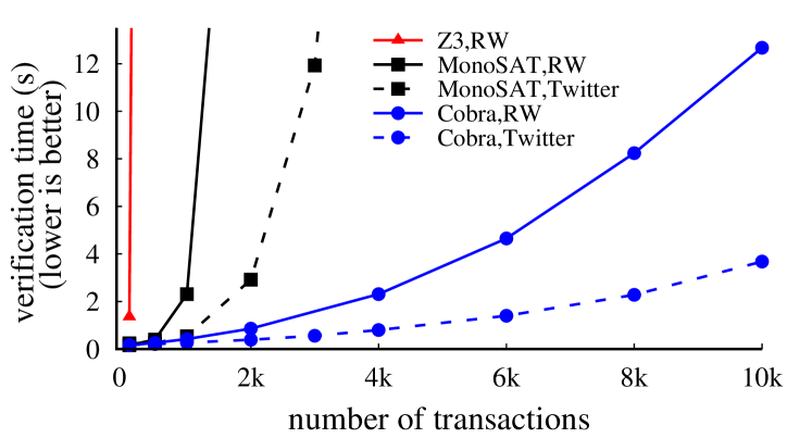
Figure 5: cobra’s running time is faster than MonoSAT’s and Z3’s on the BlindW-RW workload (solid lines) and the Twitter workload (dashed lines). The same holds on the other benchmarks (not depicted). Verification runtime grows superlinearly.

Verification runtime vs. number of transactions. We compare cobra to other baselines, on the various workloads. There are 24 clients. We vary the total number of transactions in the workload, and measure the total verification time. Figure 5 depicts the results on two benchmarks. On all five benchmarks, cobra does better than MonoSAT which does better than Z3.

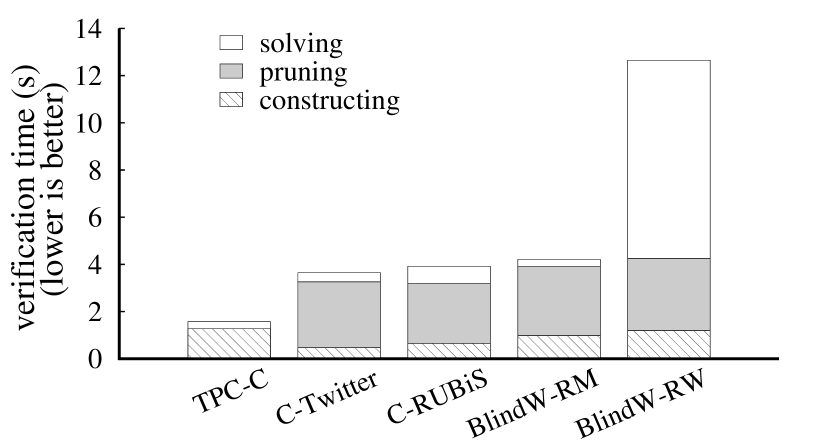
Figure 6: Decomposition of cobra runtime, on 10k-transaction workloads. In benchmarks with RMWs only (the left one), there is no constraint, so cobra doesn’t do pruning (see also footnote 3, page 3); in benchmarks with many reads and RMWs (the middle three), the dominant component is pruning not solving, because cobra’s own logic can identify concrete dependencies; in benchmarks with many blind writes (the last one), solving is a much larger contributor because cobra is not able to eliminate as many constraints.

Detecting serializability violations. In order to investigate cobra’s performance on an unsatisfiable instance: does it trigger an exhaustive search, at least on the real-world workloads we found? We evaluate cobra on five real-world workloads that are known to have serializability violations. cobra detects them in reasonable time. Figure 7 shows the results.

Violation	Database	#Txns	Time
G2-anomaly [12]	YugaByteDB 1.3.1.0	37.2k	66.3s
Disappear writes [1]	YugaByteDB 1.1.10.0	2.8k	5.0s
G2-anomaly [11]	CockroachDB-beta 20160829	446	1.0s
Read uncommitted [17]	CockroachDB 2.1	20$\star$	1.0s
Read skew [16]	FaunaDB 2.5.4	8.2k	11.4s

Figure 7: Serializability violations that cobra checks. “Violation” describes the phenomena that clients experience. “Database” is the database (with version number) that generates the violation. “#Txns” is the size of the violation history. “Time” is the runtime for cobra to detect such violation.
$\star$ The bug report only provides the history snippet that violates serializability.

Decomposition of cobra’s verification runtime. We measure the wall clock time of cobra’s verification on our setup, broken into three stages: constructing, which includes creating the graph of known edges, combining writes, and creating constraints (§3.1–§3.2); pruning (§3.3), which includes the time taken by the GPU; and solving (§3.4), which includes the time spent within MonoSAT. We experiment with all benchmarks, with 10k transactions. Figure 6 depicts the results.

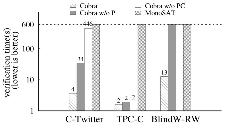
Figure 8: Differential analysis on different workloads. Log-scale, with values above bars. On C-Twitter, each of cobra’s components contributes meaningfully. On TPC-C, combining writes exploits the RMW pattern and solves all the constraints (see also footnote 3, page 3). On the other hand, pruning is essential for BlindW-RW.

Differential analysis. We experiment with four variants: cobra itself; cobra without pruning (§3.3); cobra without pruning and coalescing (§3.2), which is equivalent to MonoSAT plus write combining (§3.1); and the MonoSAT baseline. We experiment with three benchmarks, with 10k transactions. Figure 8 depicts the results.

6.2 Scaling

We want to know: what offered load (to the database) can cobra support on an ongoing basis? To answer this question, we must quantify cobra’s verification capacity, in txns/second. This depends on the characteristics of the workload, the number of transactions one round (§4) verifies ($\#tx_{r}$), and the average time for one round of verification ($t_{r}$). Note that the variable here is $\#tx_{r}$; $t_{r}$ is a function of that choice. So the verification capacity for a particular workload is defined as: $\max_{\#tx_{r}}(\#tx_{r}/t_{r})$.

To investigate this quantity, we run our benchmarks on RocksDB with 24 concurrent clients, a fence transaction every 20 transactions. We generate a 100k-transaction history ahead of time. For that same history, we vary $\#tx_{r}$, plot $\#tx_{r}/t_{r}$, and choose the optimum.

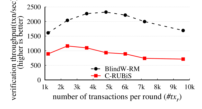
Figure 9: Verification throughput vs. round size ($\#tx_{r}$). The verification capacity for BlindW-RM (the dashed line) is 2.3k txn/sec when $\#tx_{r}$ is 5k; the capacity for C-RUBiS (the solid line) is 1.2k txn/sec when $\#tx_{r}$ is 2.5k.

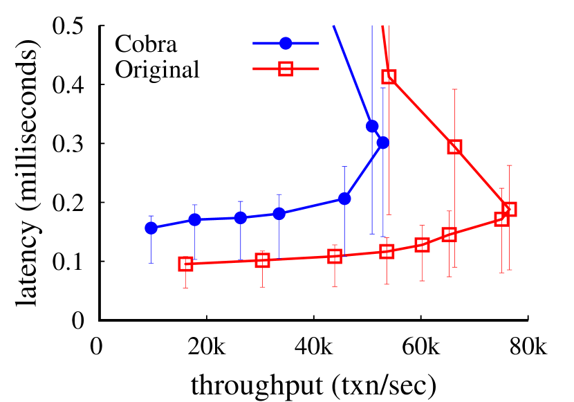
(a) RocksDB

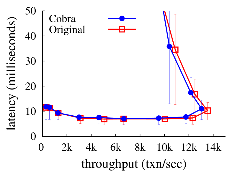
(b) PostgreSQL

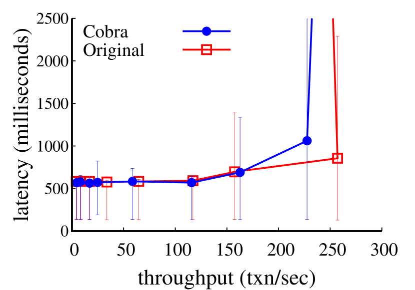
(c) Google Datastore

Figure 10: Throughput and latency, for C-Twitter benchmark. On the left is the in-process setup; 90th percentile latency increases 64%, with 31% throughput penalty, an artifact of history collection (disk bandwidth contention between clients and the DB). In the middle is the local setup (PostgreSQL), where cobra imposes minor overhead. Finally, on the right is the cloud setup; there is an artifact here too: the throughput penalty reflects a ceiling imposed by the cloud service for a fresh DB instance.

Figure 9 depicts the results. When $\#tx_{r}$ is smaller, cobra wastes cycles on redundant verification; when $\#tx_{r}$ is larger, cobra suffers from a problem size that is too large (recall that verification time increases superlinearly; §6.1). For different workloads, the optimal choices of $\#tx_{r}$ are different.

In workload BlindW-RW, cobra runs out of GPU memory. The reason is that due to many blind writes in this workload, cobra is unable to garbage collect enough transactions and fit the remaining history into the GPU memory. Our future work is to investigate this case and design a more efficient (in terms of deleting more transactions) algorithm.

6.3 cobra online overheads

The baseline in this section is the legacy system; that is, clients use the unmodified database library (for example, JDBC), with no recording of history.

Throughput latency analysis. We evaluate cobra’s client-side throughput and latency in the three setups, tuning the number of clients (up to 256) to saturate the databases. Figure 10 depicts the results.

workload	network overhead		history
	traffic	percentage	size
BWrite-RW	227.4 KB	7.28%	245.5 KB
C-Twitter	292.9 KB	4.46%	200.7 KB
C-RUBiS	107.5 KB	4.53%	148.9 KB
TPC-C	78.2 KB	2.17%	1380.8 KB

Figure 11: Network and storage overheads per one thousand transactions. The network overheads comes from fence transactions and the metadata (transaction ids and write ids) added by cobra’s client library.

Network cost and history size. We evaluate the network traffic on the client side by tracking the number of bytes sent over the NIC. We measure the history size by summing sizes of the history files. Figure 11 summarizes.

7 Related work

Below, we cover many works that wish to verify or enforce the correctness of storage, some with very similar motivations to ours. As stated earlier (§1), our problem statement is differentiated by combining requirements: (a) a black box database, (b) performance and concurrency approximating that of a cobra-less system, and (c) checking view-serializability.

Isolation testing and Consistency testing. Serializability is a particular isolation level in a transactional system—the I in ACID transactions. Because checking view-serializability is NP-complete [91], to the best of our knowledge, all works testing serializability prior to cobra are checking conflict-serializability where the write-write ordering is known. Sinha et al. [102] record the ordering of operations in a modified software transactional memory library to reduce the search space in checking serializability; this work uses the polygraph data structure (§2.3). The idea of recording order to help test serializability has also been used in detecting data races in multi-threaded programs [115, 68, 108].

In shared memory systems and systems that offer replication (but do not necessarily support transactions), there is an analogous correctness contract, namely consistency. (Confusingly, the “C(onsistency)” in ACID transactions refers to something else, namely semantic invariants [33].) Example consistency models are linearizability [71], sequential consistency [79], and eventual consistency [93].

Testing for these consistency models is an analogous problem to ours. In both cases, one searches for a schedule that fits the ordering constraints of both the model and the history [64]. As in checking serializability, the computational complexity of checking consistency decreases if a stronger model is targeted (for example, linearizability vs. sequential consistency) [63], or if more ordering information can be (intrusively) acquired (by opening black boxes) [114].

Concerto [30] uses deferred verification, allowing it to exploit an offline memory checking algorithm [43] to check online the sequential consistency of a highly concurrent key-value store. Concerto’s design achieves orders-of-magnitude performance improvement compared to Merkle tree-based approaches [88, 43], but it also requires modifications of the database. (See elsewhere [80, 57] for related algorithms.)

A body of work examines cloud storage consistency [29, 26, 84, 83]. These works rely on extra ordering information obtained through techniques like loosely- or well-synchronized clocks [29, 64, 26, 84, 76], or client-to-client communication [101, 83]. As another example, a gateway that sequences the requests can ensure consistency by enforcing ordering [101, 94, 104, 73]. Some of cobra’s techniques are reminiscent of these works, such as its use of precedence graphs [29, 64]. However, a substantial difference is that cobra neither modifies the “memory” (the database) to get information about the actual internal schedule nor depends on external synchronization. cobra of course exploits epochs for safe deletion (§4), but this is a performance optimization, not core to the verification task, and invokes standard database interfaces.

Execution integrity. Our problem relates to the broad category of execution integrity—ensuring that a module in another administrative domain is executing as expected. For example, Orochi [109] is an end-to-end audit that gives a verifier assurance that a given web application, including its database, is executing according to the code it is allegedly running. Orochi operates in a setting reminiscent of the one that we consider in this paper, in which there are collectors and an untrusted cloud service. Verena [75] operates in a similar model (but makes fewer assumptions, in that its hash server and application server are mutually distrustful); Verena uses authenticated data structures and a careful placement of function to guarantee to the deployer of a given web service, backed by a database, that the delivered web pages are correct. Orochi and Verena require that the database is strictly serializable, they provide end-to-end verification of a full stack, but they cannot treat that stack as a black box. cobra is the other way around: it of course tolerates (non-strict) serializability, its verification purview is limited to the database, but it treats the database as a black box.

Other examples of execution integrity include AVM [67] and Ripley [111], which involve checking an untrusted module by re-executing the inputs to it. These systems likewise are “full stack” but “not black box.”

Another approach is to use trusted components. For example, Byzantine fault tolerant (BFT) replication [49] (where the assumption is that a super-majority is not faulty) and TEEs (trusted execution environments, comprising TPM-based systems [96, 98, 87, 86, 92, 105, 50, 70] and SGX-based systems [37, 97, 31, 72, 100, 32, 77, 104]) ensure that the right code is running. However, this does not ensure that the code itself is right; concretely, if a database violates serializability owing to an implementation bug, neither BFT nor SGX hardware helps.

There is also a class of systems that uses complexity-theoretic and cryptographic mechanisms [119, 118, 44, 99]. None of these works handle systems of realistic scale, and only one of them [99] handles concurrent workloads. An exception is Obladi [53], which remarkably provides ACID transactions atop an ORAM abstraction by exploiting a trusted proxy that carefully manages the interplay between concurrency control and the ORAM protocol; its performance is surprisingly good (as cryptographic-based systems go) but still pays 1-2 orders of magnitude overhead in throughput and latency.

SMT solver on detecting serializability violations. Several works [90, 47, 46] propose using SMT solvers to detect serializability violations under weak consistency. The underlying problem is different: they focus on encoding static programs and the correctness criterion of weak consistency; while cobra focuses on how to encode histories more efficiently. The most relevant work [103] is to use SMT solvers to permutate all possible interleaving for a concurrent program and search for serializablility violations. Despite of different setups, our baseline implementation on Z3 (§6.1) has similar encoding and similar performance (verifying hundreds of transactions in tens of seconds).

Correctness testing for distributed systems. There is a line of research on testing the correctness of distributed systems under various failures, including network partition [27], power failures [120], and storage faults [60]. In particular, Jepsen [8] is a black-box testing framework (also an analysis service) that has successfully detected massive amount of correctness bugs in some production distributed systems. cobra is complementary to Jepsen, providing the ability to check serializability of black-box databases.

Definitions and interpretations of isolation levels. cobra of course uses precedence graphs, which are a common tool for reasoning about isolation levels [91, 41, 25]. However, isolation levels can be interpreted via other means such as excluding anomalies [39] and client-centric observations [54]; it remains an open and intriguing question whether the other definitions would yield a more intuitive and more easily-implemented encoding and algorithm than the one in cobra.

Appendix A The validity of cobra’s encoding

Recall the crucial fact in Section 2.3: an acyclic precedence graph that is compatible with a polygraph constructed from a history exists iff that history is serializable [91]. In this section, we establish the analogous statement for cobra’s encoding. We do this by following the contours of Papadimitriou’s proof of the baseline statement [91]. However cobra’s algorithm requires that we attend to additional details, complicating the argument somewhat.

A.1 Definitions and preliminaries

In this section, we define the terms used in our main argument (§A.2): history, schedule, cobra polygraph, and chains.

History and schedule. The description of histories and schedules below restates what is in section 2.1.

A history is a set of read and write operations, each of which belongs to a transaction. Each write operation in the history has a key and a value as its arguments; each read operation has a key as argument, and a value as its result. The result of a read operation is the same as the value argument of a particular write operation; we say that this read operation reads from this write operation. We assume each value is unique and can be associated to the corresponding write; in practice, this is guaranteed by cobra’s client library described in Section 5. We also say that a transaction $\textit{tx}_{i}$ reads (a key $k$) from another transaction $\textit{tx}_{j}$ if: $\textit{tx}_{i}$ contains a read rop, rop reads from write wrop on $k$, and $\textit{tx}_{j}$ contains the write wrop.

A schedule is a total order of all operations in a history. A serial schedule means that the schedule does not have overlapping transactions. A history matches a schedule if: they have the same operations, and executing the operations in schedule order on a single-copy set of data results in the same read results as in the history. So a read reading-from a write indicates that this write is the read’s most recent write (to this key) in any matching schedule.

Definition 1 (Serializable history).

A serializable history is a history that matches a serial schedule.

cobra polygraph. In the following, we define a cobra polygraph; this is a helper notion for the known graph (g in the definition below) and generalized constraints (con in the definition below) mentioned in Section 3.

Definition 2 (cobra polygraph).

Given a history $h$, a cobra polygraph $Q(h)=(\textit{g},\,\textit{con})$ where g and con are generated by ConstructEncoding from Figure 3.

We call a directed graph $\hat{g}$ compatible with a cobra polygraph $Q(h)=(\textit{g},\,\textit{con})$, if $\hat{g}$ has the same vertices as g, includes the edges from g, and selects one edge set from each constraint in con.

Definition 3 (Acyclic cobra polygraph).

A cobra polygraph $Q(h)$ is acyclic if there exists an acyclic graph that is compatible with $Q(h)$.

Chains. When constructing a cobra polygraph from a history, function CombineWrites in cobra’s algorithm (Figure 3) produces chains. One chain is an ordered list of transactions, associated to a key $k$, that (supposedly) contains a sequence of consecutive writes (defined below in Definition 5) on key $k$. In the following, we will first define what is a sequence of consecutive writes and then prove that a chain is indeed such a sequence.

Definition 4 (successive write).

In a history, a transaction $\textit{tx}_{i}$ is a successive write of another transaction $\textit{tx}_{j}$ on a key $k$, if (1) both $\textit{tx}_{i}$ and $\textit{tx}_{j}$ write to $k$ and (2) $\textit{tx}_{i}$ reads $k$ from $\textit{tx}_{j}$.

Definition 5 (A sequence of consecutive writes).

A sequence of consecutive writes on a key $k$ of length $n$ is a list of transactions $[\textit{tx}_{1},\ldots,\textit{tx}_{n}]$ for which $\textit{tx}_{i}$ is a successive write of $\textit{tx}_{i-1}$ on $k$, for $1<i\leq n$.

Although the overall problem of detecting serializability is NP-complete [91], there are local malformations, which immediately indicate that a history is not serializable. We capture two of them in the following definition:

Definition 6 (An easily rejectable history).

An easily rejectable history $h$ is a history that either (1) contains a transaction that has multiple successive writes on one key, or (2) has a cyclic known graph g of $Q(h)$.

An easily rejectable history is not serializable. First, if a history has condition (1) in the above definition, there exist at least two transactions that are successive writes of the same transaction (say $\textit{tx}_{i}$) on some key $k$. And, these two successive writes cannot be ordered in a serial schedule, because whichever is scheduled later would read $k$ from the other rather than from $\textit{tx}_{i}$. Second, if there is a cycle in the known graph, this cycle must include multiple transactions (because there are no self-loops, since we assume that transactions never read keys after writing to them). The members of this cycle cannot be ordered in a serial schedule.

Lemma 7.

cobra rejects easily rejectable histories.

Proof.

cobra (the algorithm in Figure 3 and the constraint solver) detects and rejects easily rejectable histories as follows. (1) If a transaction has multiple successive writes on the same key in $h$, cobra’s algorithm explicitly detects this case. The algorithm checks, for transactions reading and writing the same key (line 19), whether multiple of them read this key from the same transaction (line 21). If so, the transaction being read has multiple successive writes, hence the algorithm rejects (line 22). (2) If the known graph has a cycle, cobra detects and rejects this history when checking acyclicity in the constraint solver. ∎

On the other hand, if a history is not easily rejectable, we want to argue that each chain produced by the algorithm is a sequence of consecutive writes.

Claim 8.

If cobra’s algorithm makes it to line 33 (immediately before CombineWrites), then from this line on, any transaction writing to a key $k$ appears in exactly one chain on $k$.

Proof.

Prior to line 33, cobra’s algorithm loops over all the write operations (line 30–31), creating a chain for each one (line 32). As in the literature [91, 113], we assume that each transaction writes to a key only once. Thus, any tx writing to a key $k$ has exactly one write operation to $k$ and hence appears in exactly one chain on $k$ in line 33.

Next, we argue that CombineWrites preserves this invariant. This suffices to prove the claim, because after line 33, only CombineWrites updates chains (variable chains in the algorithm).

The invariant is preserved by CombineWrites because each of its loop iterations splices two chains on the same key into a new chain (line 51) and deletes the two old chains (line 50). From the perspective of a transaction involved in a splicing operation, its old chain on key $k$ has been destroyed, and it has joined a new one on key $k$, meaning that the number of chains it belongs to on key $k$ is unchanged: the number remains 1. ∎

One clarifying fact is that a transaction can appear in multiple chains on different keys, because a transaction can write to multiple keys.

Claim 9.

If cobra’s algorithm does not reject in line 22, then after CreateKnownGraph, for any two distinct entries $\textit{ent}_{1}$ and $\textit{ent}_{2}$ (in the form of $\langle\textit{key},\,\textit{tx}_{i},\,\textit{tx}_{j}\rangle$) in wwpairs: if $\textit{ent}_{1}.\textrm{key}=\textit{ent}_{2}.\textrm{key}$, then $\textit{ent}_{1}.\textrm{tx}_{i}\neq\textit{ent}_{2}.\textrm{tx}_{i}$ and $\textit{ent}_{1}.\textrm{tx}_{j}\neq\textit{ent}_{2}.\textrm{tx}_{j}$.

Proof.

First, we prove $\textit{ent}_{1}.\textrm{tx}_{i}\neq\textit{ent}_{2}.\textrm{tx}_{i}$. In cobra’s algorithm, line 23 is the only point where new entries are inserted into wwpairs. Because of the check in line 21–22, the algorithm guarantees that a new entry will not be inserted into wwpairs if an existing entry has the same $\langle\textit{key},\,\textit{tx}_{i}\rangle$. Also, existing entries are never modified. Thus, there can never be two entries in wwpairs indexed by the same $\langle\textit{key},\,\textit{tx}_{i}\rangle$.

Second, we prove $\textit{ent}_{1}.\textrm{tx}_{j}\neq\textit{ent}_{2}.\textrm{tx}_{j}$. As in the literature [91, 113], we assume that one transaction reads a key at most once. As a consequence, the body of the loop in line 19, including line 23, is executed at most once for each (key,tx) pair. Therefore, there cannot be two entries in wwpairs that match $\langle\textit{key},\textrm{\_},\textit{tx}\rangle$. ∎

Claim 10.

In one iteration of CombineWrites (line 44), for $\textit{ent}_{i}=\langle\textit{key},\,\textit{tx}_{1},\,\textit{tx}_{2}\rangle$ retrieved from wwpairs, there exist $\textit{chain}_{1}$ and $\textit{chain}_{2}$, such that $\textit{tx}_{1}$ is the tail of $\textit{chain}_{1}$ and $\textit{tx}_{2}$ is the head of $\textit{chain}_{2}$.

Proof.

Invoking Claim 8, denote the chain on key that $\textit{tx}_{1}$ is in as $\textit{chain}_{i}$; similarly, denote $\textit{tx}_{2}$’s chain as $\textit{chain}_{j}$.

Assume to the contrary that $\textit{tx}_{1}$ is not the tail of $\textit{chain}_{i}$. Then there is a transaction $\textit{tx}^{\prime}$ next to $\textit{tx}_{1}$ in $\textit{chain}_{i}$. But the only way for two transactions ($\textit{tx}_{1}$ and $\textit{tx}^{\prime}$) to appear adjacent in a chain is through the concatenation in line 51, and that requires an entry $\textit{ent}_{j}=\langle\textit{key},\,\textit{tx}_{1},\,\textit{tx}^{\prime}\rangle$ in wwpairs. Because $\textit{tx}^{\prime}$ is already in $\textit{chain}_{i}$ when the current iteration happens, $\textit{ent}_{j}$ must have been retrieved in some prior iteration. Since $\textit{ent}_{i}$ and $\textit{ent}_{j}$ appear in different iterations, they are two distinct entries in wwpairs. Yet, both of them are indexed by $\langle\textit{key},\,\textit{tx}_{1}\rangle$, which is impossible, by Claim 9.

Now assume to the contrary that $\textit{tx}_{2}$ is not the head of $\textit{chain}_{j}$. Then $\textit{tx}_{2}$ has an immediate predecessor $\textit{tx}^{\prime}$ in $\textit{chain}_{j}$. In order to have $\textit{tx}^{\prime}$ and $\textit{tx}_{2}$ appear adjacent in $\textit{chain}_{j}$, there must be an entry $\textit{ent}_{k}=\langle\textit{key},\,\textit{tx}^{\prime},\,\textit{tx}_{2}\rangle$ in wwpairs. Because $\textit{tx}^{\prime}$ is already in $\textit{chain}_{j}$ when the current iteration happens, $\textit{ent}_{k}$ must have been retrieved in an earlier iteration. So, $\textit{ent}_{k}=\langle\textit{key},\,\textit{tx}^{\prime},\,\textit{tx}_{2}\rangle$ and $\textit{ent}_{i}=\langle\textit{key},\,\textit{tx}_{1},\,\textit{tx}_{2}\rangle$ are distinct entries in wwpairs, which is impossible, by Claim 9. ∎

Lemma 11.

If $h$ is not easily rejectable, every chain is a sequence of consecutive writes after CombineWrites.

Proof.

Because $h$ is not easily rejectable, it doesn’t contain any transaction that has multiple successive writes. Hence, cobra’s algorithm does not reject in line 22 and can make it to CombineWrites.

At the beginning (immediately before CombineWrites), all chains are single-element lists (line 32). By Definition 5, each chain is a sequence of consecutive writes with only one transaction.

Assume that, before loop iteration $t$, each chain is a sequence of consecutive writes. We show that after iteration $t$ (before iteration $t+1$), chains are still sequences of consecutive writes.

If $t\leq\textrm{size}(\textit{wwpairs})$, then in line 44, cobra’s algorithm gets an entry $\langle\textit{key},\,\textit{tx}_{1},\,\textit{tx}_{2}\rangle$ from wwpairs, where $\textit{tx}_{2}$ is $\textit{tx}_{1}$’s successive write on key. Also, we assume one transaction does not read from itself (as in the literature [91, 113]), and since $\textit{tx}_{2}$ reads from $\textit{tx}_{1}$, $\textit{tx}_{1}\neq\textit{tx}_{2}$. Then, the algorithm references the chains that they are in: $\textit{chain}_{1}$ and $\textit{chain}_{2}$.

First, we argue that $\textit{chain}_{1}$ and $\textit{chain}_{2}$ are distinct chains. By Claim 8, no transaction can appear in two chains on the same key, so $\textit{chain}_{1}$ and $\textit{chain}_{2}$ are either distinct chains or the same chain. Assume they are the same chain ($\textit{chain}_{1}=\textit{chain}_{2}$). If $\textit{chain}_{1}$ ($=\textit{chain}_{2}$) is a single-element chain, then $\textit{tx}_{1}$ (in $\textit{chain}_{1}$) is $\textit{tx}_{2}$ (in $\textit{chain}_{2}$), a contradiction to $\textit{tx}_{1}\neq\textit{tx}_{2}$.

Consider the case that $\textit{chain}_{1}$ ($=\textit{chain}_{2}$) contains multiple transactions. Because $\textit{tx}_{2}$ reads from $\textit{tx}_{1}$, there is an edge $\textit{tx}_{1}\to\textit{tx}_{2}$ (generated from line 15) in the known graph of $Q(h)$. Similarly, because $\textit{chain}_{1}$ is a sequence of consecutive writes (the induction hypothesis), any transaction tx in $\textit{chain}_{1}$ reads from its immediate prior transaction, hence there is an edge from this prior transaction to tx. Since every pair of adjacent transactions in $\textit{chain}_{1}$ has such an edge, the head of $\textit{chain}_{1}$ has a path to the tail of $\textit{chain}_{1}$. Finally, by Claim 10, $\textit{tx}_{2}$ is the head of $\textit{chain}_{2}$ and $\textit{tx}_{1}$ is the tail of $\textit{chain}_{1}$, as well as $\textit{chain}_{1}=\textit{chain}_{2}$, there is a path $\textit{tx}_{2}\rightsquigarrow\textit{tx}_{1}$. Thus, there is a cycle ($\textit{tx}_{1}\to\textit{tx}_{2}\rightsquigarrow\textit{tx}_{1}$) in the known graph, so $h$ is easily rejectable, a contradiction.

Second, we argue that the concatenation of $\textit{chain}_{1}$ and $\textit{chain}_{2}$, denoted as $\textit{chain}_{1+2}$, is a sequence of consecutive writes. Say the lengths of $\textit{chain}_{1}$ and $\textit{chain}_{2}$ are $n$ and $m$ respectively. Since $\textit{chain}_{1}$ and $\textit{chain}_{2}$ are distinct sequences of consecutive writes, all transactions in $\textit{chain}_{1+2}$ are distinct and $\textit{chain}_{1+2}[i]$ reads from $\textit{chain}_{1+2}[i-1]$ for $i\in\{2,\ldots,n+m\}\setminus\{n+1\}$. For $i=n+1$, the preceding also holds, because $\textit{tx}_{1}$ is $\textit{chain}_{1}$’s tail ($=\textit{chain}_{1+2}[n]$), $\textit{tx}_{2}$ is $\textit{chain}_{2}$’s head ($=\textit{chain}_{1+2}[n+1]$), and $\textit{tx}_{2}$ is the successive write of $\textit{tx}_{1}$ ($\textit{tx}_{2}$ reads from $\textit{tx}_{1}$). Thus, $\textit{chain}_{1+2}$ is a sequence of consecutive writes, according to Definition 5.

If $t>\textrm{size}(\textit{wwpairs})$ and the loop ends, then chains don’t change. As they are sequences of consecutive writes after the final step (when $t=\textrm{size}(\textit{wwpairs})$), they still are after CombineWrites. ∎

In the following, when we refer to chains, we mean the state of chains after executing CombineWrites.

A.2 The main argument

In this section, the two theorems (Theorem 12 and 17) together prove the validity of cobra’s encoding.

Theorem 12.

If a history $h$ is serializable, then $Q(h)$ is acyclic.

Proof.

Because $h$ is serializable, there exists a serial schedule $\hat{s}$ that $h$ matches.

Claim 13.

For any transaction rtx that reads from a transaction wtx in $h$, rtx appears after wtx in $\hat{s}$.

Proof.

This follows from the definitions given at the start of the section: if rtx reads from wtx in $h$, then there is a read operation rop in rtx that reads from a write operation wrop in wtx. Thus, as stated earlier and by definition of matching, rop appears later than wrop in $\hat{s}$. Furthermore, by definition of serial schedule, transactions don’t overlap in $\hat{s}$. Therefore, all of rtx appears after all of wtx in $\hat{s}$. ∎

Claim 14.

For any pair of transactions (rtx, wtx) where rtx reads a key $k$ from wtx in $h$, no transaction $\textit{wtx}^{\prime}$ that writes to $k$ can appear between wtx and rtx in $\hat{s}$.

Proof.

Assume to the contrary that there exists $\textit{wtx}^{\prime}$ that appears in between wtx and rtx in $\hat{s}$. By Claim 13, rtx appears after wtx in $\hat{s}$. Therefore, $\textit{wtx}^{\prime}$ appears in $\hat{s}$ before rtx and after wtx. Thus, in $\hat{s}$, rtx does not return the value of $k$ written by wtx. But in $h$, rtx returns the value of $k$ written by wtx. Thus, $\hat{s}$ and $h$ do not match, a contradiction. ∎

In the following, we use $\textit{head}_{k}$ and $\textit{tail}_{k}$ as shorthands to represent, respectively, the head transaction and the tail transaction of $\textit{chain}_{k}$. And, we denote that $\textit{tx}_{i}$ appears before $\textit{tx}_{j}$ in $\hat{s}$ as $\textit{tx}_{i}<_{\hat{s}}\textit{tx}_{j}$.

Claim 15.

For any pair of chains $(\textit{chain}_{i},\,\textit{chain}_{j})$ on the same key $k$, if $\textit{head}_{i}<_{\hat{s}}\textit{head}_{j}$, then (1) $\textit{tail}_{i}<_{\hat{s}}\textit{head}_{j}$ and (2) for any transaction rtx that reads $k$ from $\textit{tail}_{i}$, $\textit{rtx}<_{\hat{s}}\textit{head}_{j}$.

Proof.

First, we prove $\textit{tail}_{i}<_{\hat{s}}\textit{head}_{j}$. If $\textit{head}_{j}\in\textit{chain}_{j}$ then $\textit{head}_{j}\not\in\textit{chain}_{i}$, by Claim 8. If $\textit{chain}_{i}$ has only one transaction (meaning $\textit{head}_{i}=\textit{tail}_{i}$), then $\textit{tail}_{i}=\textit{head}_{i}<_{\hat{s}}\textit{head}_{j}$.

Next, if $\textit{chain}_{i}$ is a multi-transaction chain, it can be written as

$$\textit{tx}_{1},\ \cdots\ \textit{tx}_{p},\,\textit{tx}_{p+1},\ \cdots\ \textit{tx}_{n}.$$

By Lemma 11, $\textit{chain}_{i}$ is a sequence of consecutive writes on $k$, so each transaction reads $k$ from its prior transaction in $\textit{chain}_{i}$. Then, by Claim 13, $\textit{tx}_{p}<_{\hat{s}}\textit{tx}_{p+1}$, for $1\leq p<n$. Now, assume to the contrary that $\textit{head}_{j}<_{\hat{s}}\textit{tail}_{i}$ ($=\textit{tx}_{n}$). Then, by the given, $\textit{tx}_{1}(=\textit{head}_{i})<_{\hat{s}}\textit{head}_{j}<_{\hat{s}}\textit{tx}_{n}$. Thus, for some $1\leq p<n$, we have $\textit{tx}_{p}<_{\hat{s}}\textit{head}_{j}<_{\hat{s}}\textit{tx}_{p+1}$. But this is a contradiction, because $\textit{tx}_{p+1}$ reads $k$ from $\textit{tx}_{p}$, and thus by Claim 14, $\textit{head}_{j}$ cannot appear between them in $\hat{s}$.

Second, we prove that any transaction rtx that reads $k$ from $\textit{tail}_{i}$ appears before $\textit{head}_{j}$ in $\hat{s}$. Assume to the contrary that $\textit{head}_{j}<_{\hat{s}}\textit{rtx}$. We have from the first half of the claim that $\textit{tail}_{i}<_{\hat{s}}\textit{head}_{j}$. Thus, $\textit{head}_{j}$ appears between $\textit{tail}_{i}$ and rtx in $\hat{s}$, which is again a contradiction, by Claim 14. ∎

Now we prove that $Q(h)$ is acyclic by constructing a compatible graph $\hat{g}$ and proving $\hat{g}$ is acyclic. We have the following fact from function Coalesce.

Fact 16.

In Coalesce, each constraint $\langle A,\,B\rangle$ is generated from a pair of chains $(\textit{chain}_{1},\,\textit{chain}_{2})$ on the same key $k$ in line 60. All edges in edge set $A$ point to $\textit{head}_{2}$, and all edges in $B$ point to $\textit{head}_{1}$. This is because all edges in $A$ have the form either $(\textit{rtx},\textit{head}_{2})$ or $(\textit{tail}_{1},\textit{head}_{2})$; see lines 67 and 71–72. Similarly by swapping $\textit{chain}_{1}$ and $\textit{chain}_{2}$ (line 61 and 62), edges in $B$ point to $\textit{head}_{1}$.

We construct graph $\hat{g}$ as follows: first, let $\hat{g}$ be the known graph of $Q(h)$. Then, for each constraint $\langle A,\,B\rangle$ in $Q(h)$, and letting $\textit{head}_{1}$ and $\textit{head}_{2}$ be defined as in Fact 16, add $A$ to $\hat{g}$ if $\textit{head}_{1}<_{\hat{s}}\textit{head}_{2}$, and otherwise add $B$ to $\hat{g}$. This process results in a directed graph $\hat{g}$.

Next, we show that all edges in $\hat{g}$ are a subset of the total ordering in $\hat{s}$; this implies $\hat{g}$ is acyclic.

First, the edges in the known graph (line 15 and 58) are a subset of the total ordering given by $\hat{s}$. Each edge added in line 15 represents that the destination vertex reads from the source vertex in $h$. By Claim 13, this ordering holds in $\hat{s}$. As for the edges in line 58, they are added to capture the fact that a read operation (in transaction rtx) that reads from a write (in transaction $\textit{chain}[i]$) is sequenced before the next write on the same key (in transaction $\textit{chain}[i+1]$), an ordering that also holds in $\hat{s}$. (This is known as an anti-dependency in the literature [25].) If this ordering doesn’t hold in $\hat{s}$, then $\textit{chain}[i+1]<_{\hat{s}}\textit{rtx}$, and thus $\textit{chain}[i]<_{\hat{s}}\textit{chain}[i+1]<_{\hat{s}}\textit{rtx}$, which contradicts Claim 14.

Second, consider the edges in $\hat{g}$ that come from constraints. Take a constraint $\langle A,B\rangle$ generated from chains $(\textit{chain}_{1},\,\textit{chain}_{2})$ on the same key. If $\textit{head}_{1}<_{\hat{s}}\textit{head}_{2}$, then by Fact 16 and construction of $\hat{g}$, all added edges have the form $(\textit{tail}_{1},\textit{head}_{2})$ or $(\textit{rtx},\textit{head}_{2})$, where rtx reads from $\textit{tail}_{1}$. By Claim 15, the source vertex of these edges appears prior to $\textit{head}_{2}$ in $\hat{s}$; thus, these edges respect the ordering in $\hat{s}$. When $\textit{head}_{2}<_{\hat{s}}\textit{head}_{1}$, the foregoing argument works the same, with appropriate relabeling. Hence, all constraint edges chosen in $\hat{g}$ are a subset of the total ordering given by $\hat{s}$. This completes the proof. ∎

Theorem 17.

If $Q(h)$ is acyclic, then the history $h$ is serializable.

Proof.

Given that $Q(h)$ is acyclic, cobra accepts $h$. Hence, by Lemma 7, $h$ is not easily rejectable. And, by Lemma 11, each chain (after CombineWrites) is a sequence of consecutive writes.

Because $Q(h)$ is acyclic, there must exist an acyclic directed graph $q$ that is compatible with $Q(h)$.

Claim 18.

If $\textit{tx}_{i}$ appears before $\textit{tx}_{j}$ in a chain $\textit{chain}_{k}$, then graph $q$ has $\textit{tx}_{i}\rightsquigarrow\textit{tx}_{j}$.

Proof.

Because $\textit{chain}_{k}$ is a sequence of consecutive writes, a transaction tx in $\textit{chain}_{k}$ reads from its immediate predecessor in $\textit{chain}_{k}$, hence there is an edge in the known graph (generated by line 15) from the predecessor to tx. Because every pair of adjacent transactions in $\textit{chain}_{k}$ has such an edge and $\textit{tx}_{i}$ appears before $\textit{tx}_{j}$ in $\textit{chain}_{k}$, $\textit{tx}_{i}\rightsquigarrow\textit{tx}_{j}$ in $Q(h)$’s known graph. As $q$ is compatible with $Q(h$), such a path from $\textit{tx}_{i}$ to $\textit{tx}_{j}$ also exists in $q$. ∎

Claim 19.

For any chain $\textit{chain}_{i}$ (on a key $k$) and any transaction $\textit{wtx}_{j}\not\in\textit{chain}_{i}$ that writes to $k$, graph $q$ has either: (1) paths from $\textit{tail}_{i}$ and transactions that read keyfrom $\textit{tail}_{i}$ (if any) to $\textit{wtx}_{j}$, or (2) paths from $\textit{wtx}_{j}$ to all the transactions in $\textit{chain}_{i}$.

Proof.

Call the chain that $\textit{wtx}_{j}$ is in $\textit{chain}_{j}$. By Claim 8, $\textit{chain}_{j}$ exists and $\textit{chain}_{j}\neq\textit{chain}_{i}$.

For $\textit{chain}_{i}$ and $\textit{chain}_{j}$, $Q(h)$ has a constraint $\langle A,\,B\rangle$ that is generated from them (line 40). This is because $\textit{chain}_{i}$ and $\textit{chain}_{j}$ touch the same key $k$, and cobra’s algorithm creates one constraint for every pair of chains on the same key (line 39). (We assume $\textit{chain}_{i}$ is the first argument of function Coalesce and $\textit{chain}_{j}$ is the second.)

First, we argue that the edges in edge set $A$ establish $\textit{tail}_{i}\rightsquigarrow\textit{head}_{j}$ and $\textit{rtx}\rightsquigarrow\textit{head}_{j}$ (rtx reads $k$ from $\textit{tail}_{i}$) in the known graph; and $B$ establishes $\textit{tail}_{j}\rightsquigarrow\textit{head}_{i}$. Consider edge set $A$. There are two cases: (i) there are reads rtx reading from $\textit{tail}_{i}$, and (ii) there is no such read. In case (i), the algorithm adds $\textit{rtx}\to\textit{head}_{j}$ for every rtx reading-from $\textit{tail}_{i}$ (line 71–72). And $\textit{rtx}\to\textit{head}_{j}$ together with the edge $\textit{tail}_{i}\to\textit{rtx}$ (added in line 15) establish $\textit{tail}_{i}\rightsquigarrow\textit{head}_{j}$. In case (ii), cobra’s algorithm adds an edge $\textit{tail}_{i}\to\textit{head}_{j}$ to $A$ (line 67), and there is no rtx in this case. Similarly, by switching $i$ and $j$ in the above reasoning (except we don’t care about the reads in this case), edges in $B$ establish $\textit{tail}_{j}\rightsquigarrow\textit{head}_{i}$.

Second, because $q$ is compatible with $Q(h)$, it either (1) contains $A$:

$$\textit{tail}_{i}/\textit{rtx} \rightsquigarrow\textit{head}_{j}$$ [proved in the first half]

$$\rightsquigarrow\textit{wtx}_{j} \textit{wtx}_{j}\in\textit{chain}_{j}$$ [Claim 18; ]

or else (2) contains $B$:

$$\textit{wtx}_{j} \rightsquigarrow\textit{tail}_{j} \textit{wtx}_{j}\in\textit{chain}_{j}$$ [Claim 18; ]

$$\rightsquigarrow\textit{head}_{i}$$ [proved in the first half]

$$\rightsquigarrow\textit{tx} \textit{tx}\in\textit{chain}_{i}$$ [Claim 18; ]

The argument still holds if $\textit{wtx}_{j}=\textit{head}_{j}$ in case (1): remove the second step in (1). Likewise, if $\textit{wtx}_{j}=\textit{tail}_{j}$ in case (2), remove the first step in (2). ∎

Claim 20.

For any pair of transactions $(\textit{wtx},\,\textit{rtx})$ where rtx reads a key $k$ from wtx and any other transaction $\textit{wtx}^{\prime}$ that writes to $k$, graph $q$ has either $\textit{wtx}^{\prime}\rightsquigarrow\textit{wtx}$ or $\textit{rtx}\rightsquigarrow\textit{wtx}^{\prime}$.

Proof.

By Claim 8, wtx must appear in some chain $\textit{chain}_{i}$ on $k$. Each of the three transactions (wtx, rtx, and $\textit{wtx}^{\prime}$) has two possibilities relative to $\textit{chain}_{i}$:

1. wtx is either the tail or non-tail of $\textit{chain}_{i}$.

2. rtx is either in $\textit{chain}_{i}$ or not.

3. $\textit{wtx}^{\prime}$ is either in $\textit{chain}_{i}$ or not.

In the following, we enumerate all combinations of the above possibilities and prove the claim in all cases.

• $\textit{wtx}=\textit{tail}_{i}$.

  Then, rtx is not in $\textit{chain}_{i}$. (If rtx is in $\textit{chain}_{i}$, its enclosing transaction would have to be subsequent to wtx in $\textit{chain}_{i}$, which is a contradiction, since wtx is last in the chain.)

  • $\textit{wtx}^{\prime}\in\textit{chain}_{i}$.

    Because wtx is the tail, $\textit{wtx}^{\prime}$ appears before wtx in $\textit{chain}_{i}$. Thus, $\textit{wtx}^{\prime}\rightsquigarrow\textit{wtx}$ in $q$ (Claim 18).

  • $\textit{wtx}^{\prime}\not\in\textit{chain}_{i}$.

    By invoking Claim 19 for $\textit{chain}_{i}$ and $\textit{wtx}^{\prime}$, $q$ either has (1) paths from each read (rtx is one of them) reading-from $\textit{tail}_{i}$ ($=\textit{wtx}$) to $\textit{wtx}^{\prime}$, therefore $\textit{rtx}\rightsquigarrow\textit{wtx}^{\prime}$. Or else $q$ has (2) paths from $\textit{wtx}^{\prime}$ to every transaction in $\textit{chain}_{i}$, and $\textit{wtx}\in\textit{chain}_{i}$, thus $\textit{wtx}^{\prime}\rightsquigarrow\textit{wtx}$.

• $\textit{wtx}\not=\textit{tail}_{i}\land\textit{wtx}\in\textit{chain}_{i}$.

  • $\textit{rtx}\in\textit{chain}_{i}$.

    Because $\textit{chain}_{i}$ is a sequence of consecutive writes on $k$ (Lemma 11) and rtx reads $k$ from wtx, rtx is the successive write of wtx. Therefore, rtx appears immediately after wtx in $\textit{chain}_{i}$.

    • $\textit{wtx}^{\prime}\in\textit{chain}_{i}$.

      Because rtx appears immediately after wtx in $\textit{chain}_{i}$, $\textit{wtx}^{\prime}$ either appears before wtx or after rtx. By Claim 18, there is either $\textit{wtx}^{\prime}\rightsquigarrow\textit{wtx}$ or $\textit{rtx}\rightsquigarrow\textit{wtx}^{\prime}$ in $q$.

    • $\textit{wtx}^{\prime}\not\in\textit{chain}_{i}$.

      By invoking Claim 19 for $\textit{chain}_{i}$ and $\textit{wtx}^{\prime}$, $q$ either has (1) $\textit{tail}_{i}\rightsquigarrow\textit{wtx}^{\prime}$, together with $\textit{rtx}\rightsquigarrow\textit{tail}_{i}$ (or $\textit{rtx}=\textit{tail}_{i}$) by Claim 18, therefore $\textit{rtx}\rightsquigarrow\textit{wtx}^{\prime}$. Or else $q$ has (2) $\textit{wtx}^{\prime}\rightsquigarrow\textit{wtx}$ ($\textit{wtx}^{\prime}$ has a path to every transaction in $\textit{chain}_{i}$, and $\textit{wtx}\in\textit{chain}_{i}$).

  • $\textit{rtx}\not\in\textit{chain}_{i}$.

    If $\textit{rtx}\not\in\textit{chain}_{i}$, because of InferRWEdges (line 53), rtx has an edge (in the known graph, hence in $q$) to the transaction that immediately follows wtx in $\textit{chain}_{i}$, denoted as $\textit{wtx}^{*}$ (and $\textit{wtx}^{*}$ must exist because wtx is not the tail of the chain).

    • $\textit{wtx}^{\prime}\in\textit{chain}_{i}$.

      Because $\textit{wtx}^{*}$ appears immediately after wtx in $\textit{chain}_{i}$, $\textit{wtx}^{\prime}$ either appears before wtx or after $\textit{wtx}^{*}$. By Claim 18, $q$ has either $\textit{wtx}^{\prime}\rightsquigarrow\textit{wtx}$ or $\textit{wtx}^{*}\rightsquigarrow\textit{wtx}^{\prime}$ which, together with edge $\textit{rtx}\to\textit{wtx}^{*}$ from InferRWEdges, means $\textit{rtx}\rightsquigarrow\textit{wtx}^{\prime}$.

    • $\textit{wtx}^{\prime}\not\in\textit{chain}_{i}$.

      By invoking Claim 19 for $\textit{chain}_{i}$ and $\textit{wtx}^{\prime}$, $q$ has either (1) $\textit{tail}_{i}\rightsquigarrow\textit{wtx}^{\prime}$ which, together with $\textit{rtx}\to\textit{wtx}^{*}$ (from InferRWEdges) and $\textit{wtx}^{*}\rightsquigarrow\textit{tail}_{i}$ (Claim 18), means $\textit{rtx}\rightsquigarrow\textit{wtx}^{\prime}$. Or else $q$ has (2) $\textit{wtx}^{\prime}\rightsquigarrow\textit{wtx}$ ($\textit{wtx}^{\prime}$ has a path to every transaction in $\textit{chain}_{i}$, and $\textit{wtx}\in\textit{chain}_{i}$).

∎

By topologically sorting $q$, we get a serial schedule $\hat{s}$. Next, we prove $h$ matches $\hat{s}$, hence $h$ is serializable (Definition 1).

Since $h$ and $\hat{s}$ have the same set of transactions (because $q$ has the same transactions as the known graph of $Q(h)$, and thus also the same as $h$), we need to prove only that for every read that reads from a write in $h$, the write is the most recent write to that read in $\hat{s}$.

First, for every pair of transactions $(\textit{wtx},\,\textit{rtx})$ such that rtx reads a key $k$ from wtx in $h$, $q$ has an edge $\textit{wtx}\to\textit{rtx}$ (added to the known graph in line 15); thus rtx appears after wtx in $\hat{s}$ (a topological sort of $q$). Second, by invoking Claim 20 for $(\textit{wtx},\,\textit{rtx})$, any other transaction writing to $k$ is either “topologically prior” to wtx or “topologically subsequent” to rtx. This ensures that, the most recent write of rtx’s read (to $k$) belongs to wtx in $\hat{s}$, hence rtx reads the value of $k$ written by wtx in $\hat{s}$ as it does in $h$. This completes the proof. ∎

Appendix B Garbage collection correctness proof

 

1:procedure VerifySerializability(history_stream)

2:   $i\leftarrow 0$; $\textit{g}\leftarrow$ empty graph

3:   $\textit{wwpairs}\leftarrow$ empty map $\{\langle\textrm{Key},\textrm{Tx}\rangle\to\textrm{Tx}\}$

4:   $\textit{readfrom}\leftarrow$ empty map $\{\langle\textrm{Key},\textrm{Tx}\rangle\to\textrm{Set}\langle\textrm{Tx}\rangle\}$

5:   while True:

6:      $i\leftarrow i+1$

7:      $h_{i}\leftarrow$ fetch a continuation from history_stream

8:      $\textit{g},\textit{readfrom},\textit{wwpairs}\leftarrow$

9:              $\mbox{{CreateKnownGraph2}}(\textit{g},\textit{readfrom},\,\textit{wwpairs},\,h_{i})$

10:      

11:      $\textit{g},\,\textit{psccs}\leftarrow\mbox{{EncodeAndSolve}}(\textit{g},\,\textit{readfrom},\,\textit{wwpairs})$

12:      

13:      $\textit{g},\textit{readfrom},\textit{wwpairs}\leftarrow\mbox{{GarbageCollection}}(\textit{g},\,\textit{psccs})$    

14:

15:procedure CreateKnownGraph2(g, readfrom,  wwpairs, $h$)

16:   for transaction tx in $h$:

17:      $\textit{g}.\textrm{Nodes}\mathrel{+}=\textit{tx}$

18:      $\textit{tx}.\textrm{frozen}=\textit{False}$

19:      for read operation rop in tx :

20:         if $\textit{rop}.\textrm{read\_from\_tx}$ not in g:  reject

21:         $\textit{g}.\textrm{Edges}\mathrel{+}=(\textit{rop}.\textrm{read\_from\_tx},\ \textit{tx})$

22:         $\textit{readfrom}[\langle\textit{rop}.\textrm{key},\,\textit{rop}.\textrm{read\_from\_tx}\rangle]\mathrel{+}=\textit{tx}$       

23:      for all Keys key that are both read and written by tx:

24:         rop $\leftarrow$ the operation in tx that reads key

25:         if $\textit{wwpairs}[\langle\textit{key},\,\textit{rop}.\textrm{read\_from\_tx}\rangle]\neq\textit{null}$:

26:            reject         

27:         $\textit{wwpairs}[\langle\textit{key},\,\textit{rop}.\textrm{read\_from\_tx}\rangle]\leftarrow\textit{tx}$          

28:   

29:   for each client $c$:

30:      $\textit{list}_{c}\leftarrow$ an ordered list of trsanctions issued by $c$ in g

31:      for $i$ in $[0,\,\textrm{length}(\textit{list}_{c})-2]$:

32:         $\textit{g}.\textrm{Edges}\mathrel{+}=(\textit{list}_{c}[i],\textit{list}_{c}[i+1])$          

33:   

34:   return $\textit{g},\,\textit{readfrom},\,\textit{wwpairs}$

35:

36:procedure EncodeAndSolve($\textit{g},\,\textit{readfrom},\,\textit{wwpairs}$)

37:   $\textit{con}\leftarrow\mbox{{GenConstraints}}(g,\,\textit{readfrom},\,\textit{wwpairs})$

38:   $\textit{con},\,\textit{g}\leftarrow\mbox{{Prune}}(\textit{con},\,\textit{g})$

39:   

40:   $\textit{formula}\leftarrow\mbox{{EncodeSMT}}(\textit{con},\,\textit{g})$

41:   $\textit{solved}\leftarrow$ MonoSAT.solve(formula)

42:   if not solved: reject

43:   

44:   $\textit{psccs}\leftarrow\mbox{{GenPolySCCs}}(\textit{con},\,\textit{g})$

45:   return g, psccs

46:

47:procedure GenPolySCCs($\textit{con},\,\textit{g}$)

48:   $g^{\prime}\leftarrow g$

49:   $g^{\prime}.\textrm{Edges}\leftarrow g^{\prime}.\textrm{Edges}\ \cup$ {all edges in con}

50:   $\textit{psccs}\leftarrow\mbox{{CalcStronglyConnectedComponents}}(g^{\prime})$

51:   return psccs

52:

53:procedure GarbageCollection(g, psccs)

54:   $\textit{epoch}_{\textrm{agree}}\leftarrow\mbox{{AssignEpoch}}(\textit{g})$

55:   $\mbox{{SetFrozen}}(\textit{g},\,\textit{epoch}_{\textrm{agree}})$

56:   $\mbox{{Set\xmakefirstuc{obsolete}}}(\textit{g},\,\textit{epoch}_{\textrm{agree}})$

57:   $\mbox{{Set\xmakefirstuc{removable}}}(\textit{g},\,\textit{psccs})$

58:   return $\mbox{{SafeDeletion2}}(\textit{g},\,\textit{readfrom},\,\textit{wwpairs})$

59:procedure AssignEpoch(g)

60:   $\textit{epoch\_num}\leftarrow 0$

61:   $\textit{topo\_tx}\leftarrow\textrm{TopologicalSort}(\textit{g})$

62:   for tx in topo_tx:

63:      if tx writes to key “EPOCH”:

64:         $\textit{tx}.\textrm{epoch}\leftarrow\textit{epoch\_num}$

65:         $\textit{epoch\_num}\leftarrow\textit{epoch\_num}+1$          

66:   for tx in topo_tx:

67:      if tx reads but not writes key “EPOCH”:

68:         $\textit{tx}.\textrm{epoch}\leftarrow\textit{tx}.\textrm{read\_from\_tx}.\textrm{epoch}$          

69:   

70:   $\textit{epoch}_{\textrm{agree}}\leftarrow\inf$

71:   for each client $c$:

72:      $\textit{list}_{c}\leftarrow$ an ordered list of trsanctions issued by $c$ in g

73:      $\textit{rlist}_{c}\leftarrow$ reversed ordered list of $\textit{list}_{c}$

74:      $\textit{cur\_epoch}\leftarrow\inf$

75:      for tx in $\textit{rlist}_{c}$:

76:         if tx touches key “EPOCH”:

77:            if $\textit{cur\_epoch}=\inf$:

78:               $\textit{epoch}_{\textrm{agree}}\leftarrow\textrm{min}(\textit{epoch}_{\textrm{agree}},\,\textit{tx}.\textrm{epoch})$             

79:            $\textit{cur\_epoch}\leftarrow$ $\textit{tx}.\textrm{epoch}$

80:         else:

81:            $\textit{tx}.\textrm{epoch}=(\textit{cur\_epoch}=\inf\ ?\ \inf:\textit{cur\_epoch}-1)$                   

82:   return $\textit{epoch}_{\textrm{agree}}$

83:

84:procedure SetFrozen(g, $\textit{epoch}_{\textrm{agree}}$)

85:   $\textit{fepoch}\leftarrow\textit{epoch}_{\textrm{agree}}-2$

86:   for tx in g :

87:      if $\textit{tx}.\textrm{epoch}\leq\textit{fepoch}$ and

88:          all predecssors of tx in g have epoch $\leq\textit{fepoch}$:

89:         $\textit{tx}.\textrm{frozen}\leftarrow\textit{True}$          

90:

91:procedure Setobsolete(g, $\textit{epoch}_{\textrm{agree}}$)

92:   $\textit{fepoch}\leftarrow\textit{epoch}_{\textrm{agree}}-2$

93:   for tx in g :

94:      if $\textit{tx}.\textrm{epoch}\leq\textit{fepoch}$:

95:         $\textit{obsolete}\leftarrow\textit{True}$

96:         for Key key that tx writes:

97:            if $\not\exists tx_{j},\ s.t.\ \textit{tx}\rightsquigarrow\textit{tx}_{j}\land\textit{tx}_{j}.\textrm{epoch}\leq\textit{fepoch}\land\textit{tx}_{j}\textrm{ writes }\textit{key}$:

98:               $\textit{obsolete}\leftarrow\textit{False}$; break                      

99:         $\textit{tx}.\textrm{obsolete}\leftarrow\textit{obsolete}$          

100:

101:procedure Setremovable($\textit{g},\,\textit{psccs}$)

102:   for tx in g :

103:      if $\textit{tx}.\textrm{frozen}=\textit{True}$:

104:         if $\textit{tx}.\textrm{obsolete}=\textit{True}$ or tx is read-only:

105:            $\textit{tx}.\textrm{candidate}\leftarrow\textit{True}$                   

106:   for pscc in psccs:

107:      if $\forall\textit{tx}\in\textit{pscc},\ \textit{tx}.\textrm{candidate}=\textit{True}$:

108:         for tx in pscc:

109:            $\textit{tx}.\textrm{removable}\leftarrow\textit{True}$                   

110:

111:procedure SafeDeletion2($\textit{g},\,\textit{readfrom},\,\textit{wwpairs}$)

112:   for tx in g :

113:      if $\textit{tx}.\textrm{removable}=\textit{True}$ and tx doesn’t touch key “EPOCH”:

114:         $\textit{g}.\textrm{Nodes}\mathrel{-}=\textit{tx}$

115:         $\textit{g}.\textrm{Edges}\mathrel{-}=\{\textrm{edges with {tx} as one endpoint}\}$

116:         $\textit{readfrom}\mathrel{-}=\{\textrm{tuples containing {tx}}\}$

117:         $\textit{wwpairs}\mathrel{-}=\{\textrm{tuples containing {tx}}\}$          

118:   return $\textit{g},\textit{readfrom},\textit{wwpairs}$

 

Figure 12: cobra’s algorithm for verification in rounds.

B.1 Verification in rounds

Besides the “one-shot verification” described in §3 and Appendix A, cobra also works for online verification and does verification in rounds (pseudocode is described in Figure 12). In each round, cobra’s verifier checks serializability on the transactions that have been received. In the following, we define terms used in the context of verification in rounds: complete history, continuation, strong session serializable, and extended history.

Complete history and continuation. A complete history is a prerequisite of checking serializability. If a history is incomplete and some of the transactions are unknown, it is impossible to decide whether this history is serializable.

Definition 21 (Complete history).

A complete history is a history where all read operations read from the write operations in the same history.

For verification in rounds, in each round, cobra’s verifier receives a set of transactions that may read from the transactions in prior rounds. We call such newly coming transactions a continuation [66].

Definition 22 (Continuation).

A continuation $r$ of a complete history $h$ is a set of transactions in which all the read operations read from transactions in either $h$ or $r$.

We denote the combination of a complete history $h$ and its continuation $r$ as $h\circ r$. By Definition 21, $h\circ r$ is also a complete history. Also, we call the transactions in future continuations of the current history as future transactions.

In the following discussion, we assume that the transactions received in each round are continuations of the known history. However, in practice, the received transactions may not form a complete history and cobra’s verifier has to adopt a preprocessing phase to filter out the transactions whose predecessors are unknown and save them for future rounds (for simplicity, such preprocessing is omitted in Figure 12 which should have happen in line 7.)

strong session serializable. As mentioned in §4.2, transactions’ serialization order in practice should respect their causality which, in our context, is the transaction issuing order by clients (or session). So, if a history satisfies serializability (Definition 1) and the corresponding serial schedule preserves the transaction issuing order, we say this history is strong session serializable, defined below.

Definition 23 (strong session serializable history).

A strong session serializable history is a history that matches a serial schedule $\hat{s}$, such that $\hat{s}$ preserves the transaction issuing order for any client.

Notice that cobra requires that each client is single-threaded and blocking (§2). So, for one client, its transaction issuing order is the order seen by the corresponding history collector (one client connects to one collector). The verifier also knows such order by referring to the history fragments.

extended history. In the following, we define a helper notion extended history that contains the information of a history that has parsed by cobra’s algorithm. An extended history $e$ of a history $h$ is a tuple $(\textit{g},\,\textit{readfrom},\,\textit{wwpairs})$ generated by CreateKnownGraph2 in Figure 12, line 9.

Notice that in cobra’s algorithm each round reuses the extended history $e=(\textit{g},\,\textit{readfrom},\,\textit{wwpairs})$ from the preceding round. In the following, we use $E(e,h)$ to represent $\textsc{\mbox{{CreateKnownGraph2}}}(\textit{g},\textit{readfrom},\textit{wwpairs},h)$. And, we use $E(h)$ as a shortened form of $E(\emptyset,h)$.

Fact 24.

For a complete history $h$ and its continuation $r$, $E(h\circ r)=E(E(h),r)$. Because readfrom and wwpairs only depend on the information carried by each transaction, and this information is the same no matter whether processing $h$ and $r$ together or separately. For client ordering edges (Figure 12, line 29–32), since they are the ordering of transactions seen by the collectors, the edges remain the same as well.

Definition 25 (Deletion from an extended history).

A deletion of a transaction $\textit{tx}_{i}$ from an extended history $E(h)$ is to (1) delete the vertex $\textit{tx}_{i}$ and edges containing $\textit{tx}_{i}$ from the known graph g in $E(h)$; and (2) delete tuples that include $\textit{tx}_{i}$ from readfrom and wwpairs.

We use $E(h)\ominus\textit{tx}_{i}$ to denote deleting $\textit{tx}_{i}$ from extended history $E(h)$.

B.2 polygraph, cobra polygraph, pruned polygraph, and pruned cobra polygraph

Notice that an extended history contains all information from a history. So, instead of building from a history, both polygraph (§2.3) and cobra polygraph (Definition 2) can be built from an extended history.

Specifically, constructing a polygraph $(V,\,E,\,C)$ from an extended history $E(h)$ works as follows (which is similar to what is in §2.3):

• $V$ are all vertices in $E(h).\textit{g}$.

• $E=\{(\textit{tx}_{i},\,\textit{tx}_{j})\ |\ \langle\,\textrm{\_},\,\textit{tx}_{i},\,\textit{tx}_{j}\,\rangle\in E(h).\textit{readfrom}\}$; that is, $\textit{tx}_{i}\xrightarrow[]{\text{wr(x)}}\textit{tx}_{j}$, for some $x$.

• $C=\{\langle\,(\textit{tx}_{j},\,\textit{tx}_{k}),\ (\textit{tx}_{k},\,\textit{tx}_{i})\,\rangle\mid(\textit{tx}_{i}\xrightarrow[]{\text{wr(x)}}\textit{tx}_{j})\,\land\,\\ \hskip 30.00005pt(\textit{tx}_{k}\textrm{\ writes to $x$})\land\textit{tx}_{k}\neq\textit{tx}_{i}\land\textit{tx}_{k}\neq\textit{tx}_{j}\}$.

We denote the polygraph generated from extended history $E(h)$ as $P(E(h))$.

Since constructing an extended history is part of cobra’s algorithm, it is natural to construct a cobra polygraph from an extended history, which works as follow: assign cobra polygraph’s known graph to be $E(h).\textit{g}$ and generate constraints by invoking

$$\textsc{\mbox{{GenConstraints}}}(E(h).\textit{g},\,E(h).\textit{readfrom},\,E(h).\textit{wwpairs}).$$

We denote the cobra polygraph generated from extended history $E(h)$ as $Q(E(h))$.

In order to test strong session serializability, we add cliens’ transaction issuing order to polygraph and cobra polygraph by inserting edges for transactions that are issued by the same client. We call such edges client ordering edges (short as CO-edges). For each client, these CO-edges point from one transaction to its immediate next transaction (Figure 12, line 29–32).

Lemma 26.

For a serializable history $h$, a serial schedule that $h$ matches is some topological sort of an acyclic graph that is compatible with the polygraph without CO-edges (and cobra polygraph without CO-edges) of $h$; and topological sorting an acyclic graph that is compatible with the polygraph without CO-edges (and cobra polygraph without CO-edges) of $h$ results in a serial schedules that $h$ matches.

Proof.

First, we prove the Lemma for polygraph (then later cobra polygraph). In Papadimitriou’s proof [91] (§3, Lemma 2), when proving that $h$ is serializable $\Rightarrow$ polygraph is acyclic, the proof constructs an acyclic compatible graph according to a serial schedule, which means that this serial schedule is a topological sort of the constructed comptible graph. On the other hand, when proving that polygraph is acyclic $\Rightarrow$ $h$ is serializable, the proof gets the serial schedule from topological sorting an ayclic compatible graph.

Similarly, for cobra polygraph, in Thoerem 12 (Appendix A), the proof constructs an acyclic compatible graph from a serial schedule; and in Thoerem 17, the proof topologically sorts an acyclic compatible graph to generate a serial schedule. ∎

In the following, all polygraphs $P(E(h))$ and cobra polygraphs $Q(E(h))$ include client ordering edges by default.

Lemma 27.

Given a complete history $h$ and its extended history $E(h)$, the following logical expressions are equivalent:

1. history $h$ is strong session serializable.

2. polygraph $P(E(h))$ is acyclic.

3. cobra polygraph $Q(E(h))$ is acyclic.

Proof.

First, we prove that $(1)\iff(2)$.

$(1)\implies(2)$: Because $h$ is strong session serializable, there exists a serial schedule $\hat{s}$ that $h$ matches and preserves the transaction issuing order of clients. By Lemma 26, $\hat{s}$ is one of the topological sorts of some graph $\hat{g}$ that is compatible with the polygraph without client ordering edges. By adding client ordering edges to $\hat{g}$, we get $\hat{g+}$. Graph $\hat{g+}$ is still compatible with $P(E(h))$, because edges of $\hat{g+}$ are a subset of the total ordering of $\hat{s}$ ($\hat{s}$ preserves the clients’ transaction issuing order). Thus, $\hat{g+}$ is acyclic, hence $P(E(h))$ is also acyclic.

$(2)\implies(1)$: Because polygraph $P(E(h))$ is acyclic, there exists a compatible graph $\hat{g+}$ that is acyclic. By removing all the client ordering edges from $\hat{g+}$, we have $\hat{g}$ which is compatible with the polygraph without client ordering edges. Because $\hat{g}$ has the same nodes but less edges than $\hat{g+}$, a topological sort $\hat{s}$ of $\hat{g+}$ is also a topological sort of $\hat{g}$. By Lemma 26, $\hat{s}$ is a serial schedule that $h$ matches. Because $\hat{g+}$ has client ordering edges, $\hat{s}$ preserves transaction issuing order of clients, hence $h$ is strong session serializable.

Similarly, we can prove $(1)\iff(3)$ by replacing polygraph (with and without client ordering edges) with cobra polygraph (with and without client ordering edges). ∎

Pruned (cobra) polygraph. Given a cobra polygraph $Q(E(h))=(\textit{g},\,\textit{con})$, we call the cobra polygraph after invoking $\textsc{\mbox{{Prune}}}(\textit{con},\,\textit{g})$ (Figure 3, line 75) as a pruned cobra polygraph, denoted as $Q_{p}(E(h))$. Similarly, if we treat a constraint in a polygraph (for example $\langle\textit{tx}_{i}\to\textit{tx}_{j},\textit{tx}_{j}\to\textit{tx}_{k}\rangle$) as a constraint in cobra polygraph but with each edge set having only one edge ($\langle\{\textit{tx}_{i}\to\textit{tx}_{j}\},\{\textit{tx}_{j}\to\textit{tx}_{k}\}\rangle$), then we can apply Prune to a polygraph $P(E(h))$ and get a pruned polygraph, denoted as $P_{p}(E(h))$.

Note that $Q(E(h))$ and $Q_{p}(E(h))$ are what cobra’s algorithm actually creates; $P(E(h))$ and $P_{p}(E(h))$ are helper notions for the proof only—they are not actually materialized.

Lemma 28.

$Q(E(h))$ is acyclic $\iff$ $Q_{p}(E(h))$ is acyclic, and $P(E(h))$ is acyclic $\iff$ $P_{p}(E(h))$ is acyclic.

Proof.

First, we prove $Q(E(h))$ is acyclic $\iff$ $Q_{p}(E(h))$ is acyclic.

“$\Rightarrow$”. To begin with, we prove that pruning one constraint $\langle A,B\rangle$ from $Q(E(h))$ does not affect the acyclicity of the remaining cobra polygraph. If so, pruning multiple constraints on an acyclic cobra polygraph still results in an acyclic cobra polygraph.

Now, consider the constraint $\langle A,B\rangle$ ($A$ and $B$ are edge sets) that has been pruned in $Q(E(h))$, and assume it gets pruned because of an edge $(\textit{tx}_{i},\textit{tx}_{j})\in A$ such that $\textit{tx}_{j}\rightsquigarrow\textit{tx}_{i}$ in the known graph.

Because $Q(E(h))$ is acyclic, there exists a compatible graph $\hat{g}$ that is acyclic. For the binary choice of $\langle A,B\rangle$, $\hat{g}$ must choose $B$; otherwise $\hat{g}$ would have a cycle due to the edge $(\textit{tx}_{i},\textit{tx}_{j})$ in $A$ and $\textit{tx}_{j}\rightsquigarrow\textit{tx}_{i}$ in the known graph. And, Prune (Figure 3, line 78–84) does the same thing—add edges in $B$ to $Q_{p}(E(h))$’s known graph, when the algorithm detects edges in $A$ conflict with the known graph. Hence, $\hat{g}$ is compatible with $Q_{p}(E(h))$ and $Q_{p}(E(h))$ is acyclic.

“$\Leftarrow$”. Because $Q_{p}(E(h))$ is acyclic, there exists a compatible graph $\hat{g^{\prime}}$ that is acyclic. Consider all constraints in $Q(E(h))$: for the pruned constraints, $\hat{g^{\prime}}$ contains edges from one of the two edge sets in the constraint; for those constraints that is not pruned, $Q_{p}(E(h))$ has them and $\hat{g^{\prime}}$ selects one edge set from each of them ($\hat{g^{\prime}}$ is compatible with $Q_{p}(E(h))$). Thus, $\hat{g^{\prime}}$ contains one edge set from all constraints in $Q(E(h))$, so it is compatible with $Q(E(h))$. Plus, $\hat{g^{\prime}}$ is acyclic, hence $Q(E(h))$ is acyclic.

Now we prove that $P(E(h))$ is acyclic $\Leftrightarrow$ $P_{p}(E(h))$ is acyclic. Because the constraint in a polygraph is a specialization of the constraint in a cobra polygraph (each edge set only contains one edge), the above argument is still true by replacing $Q(E(h))$, $Q_{p}(E(h))$ to $P(E(h))$, $P_{p}(E(h))$ respectively. ∎

Lemma 29.

Given a history that is strong session serializable, for any two transactions $\textit{tx}_{i}$ and $\textit{tx}_{j}$, $\textit{tx}_{i}\rightsquigarrow\textit{tx}_{j}$ in the known graph of $P_{p}(E(h))$ $\iff$ $\textit{tx}_{i}\rightsquigarrow\textit{tx}_{j}$ in the known graph of $Q_{p}(E(h))$

Proof.

Because $h$ is not easily rejectable, $E(h)$’s known graph is acyclic and both $P_{p}(E(h))$ and $Q_{p}(E(h))$’s known graphs contain edges in $E(h)$’s known graph.

“$\Rightarrow$”. We prove that for any edge $\textit{tx}_{a}\to\textit{tx}_{b}$ in path $\textit{tx}_{i}\rightsquigarrow\textit{tx}_{j}$ of $P_{p}(E(h))$ ($\textit{tx}_{a}$ might be $\textit{tx}_{i}$ and $\textit{tx}_{b}$ might be $\textit{tx}_{j}$), there always exists $\textit{tx}_{a}\rightsquigarrow\textit{tx}_{b}$ in $Q_{p}(E(h))$. In $P_{p}(E(h))$ and $Q_{p}(E(h))$’s known graph, there are four types of edges. Three of them—reading-from edges (Figure 12, line 21), anti-dependency edge (Figure 3, line 58), and client order edges (Figure 12, line 32)—are captured by $E(h)$’s known graph which shared by both $P_{p}(E(h))$ and $Q_{p}(E(h))$. Hence, if $P_{p}(E(h))$’s known graph has $\textit{tx}_{a}\to\textit{tx}_{b}$, $Q_{p}(E(h))$ also has it.

Next, we prove that when edge $\textit{tx}_{a}\to\textit{tx}_{b}$ is the last type: edges added by Prune (Figure 3, line 80,83) in $P_{p}(E(h))$, $Qp(E(h))$’s known graph also has $\textit{tx}_{a}\rightsquigarrow\textit{tx}_{b}$.

Consider a constraint in $P_{p}(E(h))$ is $\langle\textit{tx}_{\textrm{r}}\to\textit{tx}_{\textrm{w2}},\textit{tx}_{\textrm{w2}}\to\textit{tx}_{\textrm{w1}}\rangle$ where $\textit{tx}_{\textrm{w1}}$ and $\textit{tx}_{\textrm{w2}}$ writes to the same key; $\textit{tx}_{\textrm{r}}$ reads this key from $\textit{tx}_{\textrm{w1}}$. For $\textit{tx}_{\textrm{w1}}$ and $\textit{tx}_{\textrm{w2}}$ in $Q_{p}(E(h))$, because they write the same key, they are either (1) in the same chain, or else (2) $\textit{tx}_{\textrm{w2}}$ and $\textit{tx}_{\textrm{w2}}$ belong to two chains and there is a constraint about these two chains.

Given $\textit{tx}_{a}\to\textit{tx}_{b}$ is added by pruning a constraint in $P_{p}(E(h))$, there are two possibilities:

• $\textit{tx}_{a}\to\textit{tx}_{b}$ is $\textit{tx}_{\textrm{r}}\to\textit{tx}_{\textrm{w2}}$, which means $\textit{tx}_{\textrm{w1}}\rightsquigarrow\textit{tx}_{\textrm{w2}}$ (otherwise, the constraint would not be pruned). In $Q_{p}(E(h))$, for above case (1), because $\textit{tx}_{\textrm{w1}}\rightsquigarrow\textit{tx}_{\textrm{w2}}$, $\textit{tx}_{\textrm{r}}$ reading from $\textit{tx}_{\textrm{w1}}$ has paths to the successive transactions (including $\textit{tx}_{\textrm{w2}}$) in the chain; for (2), because $\textit{tx}_{\textrm{w1}}\rightsquigarrow\textit{tx}_{\textrm{w2}}$, this constraint would be pruned and $\textit{tx}_{\textrm{r}}\rightsquigarrow\textit{tx}_{\textrm{w2}}$.

• $\textit{tx}_{a}\to\textit{tx}_{b}$ is $\textit{tx}_{\textrm{w2}}\to\textit{tx}_{\textrm{w1}}$, which means $\textit{tx}_{\textrm{w2}}\rightsquigarrow\textit{tx}_{\textrm{r}}$. In $Q_{p}(E(h))$, for (1), $\textit{tx}_{\textrm{w2}}$ must appear earlier than $\textit{tx}_{\textrm{w1}}$ in the chain (hence $\textit{tx}_{\textrm{w2}}\rightsquigarrow\textit{tx}_{\textrm{r}}$), because otherwise $\textit{tx}_{\textrm{r}}\rightsquigarrow\textit{tx}_{\textrm{w2}}$, a contradiction; for (2), because $\textit{tx}_{\textrm{w2}}\rightsquigarrow\textit{tx}_{\textrm{r}}$, the tail of chain that $\textit{tx}_{\textrm{w2}}$ is in has a path to the head of $\textit{tx}_{\textrm{w1}}$’s chain, hence $\textit{tx}_{\textrm{w2}}\rightsquigarrow\textit{tx}_{\textrm{w1}}$ in $Q_{p}(E(h))$.

“$\Leftarrow$”. Similarly, by swapping $P_{p}(E(h))$ and $Q_{p}(E(h))$ in the above argument, we need to prove that given a pruned constraint $\langle A,B\rangle$ in $Q_{p}(E(h))$ which contains $\textit{tx}_{a}\to\textit{tx}_{b}$, there exists $\textit{tx}_{a}\rightsquigarrow\textit{tx}_{b}$ in $P_{p}(E(h))$.

Again, for a constraint $\langle A,B\rangle$ about two chains $\textit{chain}_{i}$ and $\textit{chain}_{j}$ in $Q_{p}(E(h))$ ($\textit{head}_{i}$/$\textit{tail}_{i}$ is the head/tail of $\textit{chain}_{i}$; $\textit{rtx}_{i}$ is a read transaction reads from $\textit{tail}_{i}$). There are two possibilities:

• $\textit{tx}_{a}\to\textit{tx}_{b}$ is $\textit{rtx}_{i}\to\textit{head}_{j}$, which means $\textit{head}_{i}\rightsquigarrow\textit{tail}_{j}$. Consider the constraint $\langle\textit{rtx}_{i}\to\textit{head}_{j},\textit{head}_{j}\to\textit{tail}_{i}\rangle$ in $P_{p}(E(h))$. Given that $h$ is serializable, two chains must be schedule sequentially and cannot overlap, hence $\textit{tail}_{i}\rightsquigarrow\textit{head}_{j}$. Then, this constraint in $P_{p}(E(h))$ would be pruned and there is an edge $\textit{rtx}_{i}\to\textit{head}_{j}$.

• $\textit{tx}_{a}\to\textit{tx}_{b}$ is $\textit{tail}_{i}\to\textit{head}_{j}$, which means $\textit{head}_{i}\rightsquigarrow\textit{tail}_{j}$. Call the second last transaction in $\textit{chain}_{i}$ $\textit{tx}_{k}$. Consider the constraint $\langle\textit{tail}_{i}\to\textit{head}_{j},\textit{head}_{j}\to\textit{tx}_{k}\rangle$ ($\textit{tail}_{i}$ reads from $\textit{tx}_{k}$). Again, because $h$ is serializable, two chains cannot overlap, and $\textit{tx}_{k}\rightsquigarrow\textit{head}_{j}$. Thus, the constraint is pruned and $P_{p}(E(h))$ has $\textit{tail}_{i}\to\textit{head}_{j}$.

∎

(Extended) easily rejectable history. Given that a cobra polygraph $Q(E(h))$ and a pruned cobra polygraph $Q_{p}(E(h))$ are equivalent in acyclicity, we extend the definition of an easily rejectable history (Definition 6) to use $Q_{p}(E(h))$ which rules out more local malformations that are not strong session serializable.

Definition 30 (An easily rejectable history).

An easily rejectable history $h$ is a history that either (1) contains a transaction that has multiple successive writes on one key, or (2) has a cyclic known graph g in $Q_{p}(E(h))$.

Corollary 31.

cobra rejects (extended) easily rejectable histories.

Proof.

By Lemma 7, cobra rejects a history when (1) it contains a transaction that has multiple successive writes one one key; (2) If the known graph has a cycle in the known graph of $Q_{p}(E(h))$, cobra detects and rejects this history when checking acyclicity in the constraint solver. ∎

B.3 poly-strongly connected component

In this section, we define poly-strongly connected components (short as P-SCC) which capture the possible cycles that are generated from constraints. Intuitively, if two transactions appears in one P-SCC, it is possible (but not certian) there are cycles between them; but if these two transactions do not belong to the same P-SCC, it is impossible to have a cycle including both transactions.

Definition 32 (poly-strongly connected component).

Given a history $h$ and its pruned cobra polygraph $Q_{p}(E(h))$, the poly-strongly connected components are the strongly connected components of a directed graph that is the known graph with all edges in the constraints added to it.

Lemma 33.

In a history $h$ that is not easily rejectable, for any two transactions $\textit{tx}_{i}$ and $\textit{tx}_{j}$ writing the same key, if $\textit{tx}_{i}\not\rightsquigarrow\textit{tx}_{j}$ and $\textit{tx}_{j}\not\rightsquigarrow\textit{tx}_{i}$ in the known graph of $Q_{p}(E(h))$, then $\textit{tx}_{i}$ and $\textit{tx}_{j}$ are in the same P-SCC.

Proof.

By Claim 8, each of $\textit{tx}_{i}$ and $\textit{tx}_{j}$ appears and only appears in one chain (say $\textit{chain}_{i}$ and $\textit{chain}_{j}$ respectively). Because $\textit{tx}_{i}\not\rightsquigarrow\textit{tx}_{j}$ and $\textit{tx}_{j}\not\rightsquigarrow\textit{tx}_{i}$, $\textit{chain}_{i}\neq\textit{chain}_{j}$. cobra’s algorithm generates a constraint for every pair of chains on the same key (Figure 3, line 39), so there is a constraint $\langle A,B\rangle$ for $\textit{chain}_{i}$ and $\textit{chain}_{j}$, which includes $\textit{tx}_{i}$ and $\textit{tx}_{j}$.

Consider this constraint $\langle A,B\rangle$. One of the two edge sets ($A$ and $B$) contains edges that establish a path from the tail of $\textit{chain}_{i}$ to the head of $\textit{chain}_{j}$—either a direct edge (Figure 3, line 67), or through a read transaction that reads from the tail of $\textit{chain}_{i}$ (Figure 3, line 72). Similarly, the other edge set establishes a path from the tail of $\textit{chain}_{j}$ to the head of $\textit{chain}_{i}$. In addition, by Lemma 11, in each chain, there is a path from its head to its tail through the reading-from edges in the known graph (Figure 3, line 15). Thus, there is a cycle involving all transactions of these two chains. By Definition 32, all the transactions in these two chains—including $\textit{tx}_{i}$ and $\textit{tx}_{j}$—are in one P-SCC. ∎

B.4 Fence transaction, epoch, obsolete transaction, and frozen transaction

The challenge of garbage collecting transactions is that strong session serializability does not respect real-time ordering across clients and it is unclear to the verifier which transactions can be safely deleted from the history (§4.1). cobra uses fence transactions and epochs which generate obsolete transactions and frozen transactions that address this challenge.

Fence transactions. As defined in §4.2, fence transactions are predefined transactions that are periodically issued by each client and access a predefined key called the epoch key. Based on the value read from the epoch key, a fence transaction is either a write fence transaction (short as Wfence) or a read fence transaction (short as Rfence): Wfences read-and-modify the epoch key; and Rfences only read the epoch key. In a complete history, we define that the fence transactions are well-formed as follows.

Definition 34 (well-formed fence transactions).

In a history, fence transactions are well-formed when (1) all write fence transactions are a sequence of consecutive writes to the epoch key; and (2) all read fence transactions read from known write fence transactions.

Claim 35.

Given a complete history $h$ that is not easily rejectable, fence transactions in $h$ are well-formed.

Proof.

First, we prove that all Wfences are a sequence of consecutive writes. Because the epoch key is predefined and reserved for fence transactions, Wfences are the only transactions that update this key. Given that Wfences read-modify-write the epoch key, a Wfence read from either another Wfence or the (abstract) initial transaction if the epoch key hasn’t been created.

Given that $h$ is not easily rejectable, by Definition 30, there is no cycle in the known graph. Hence, if we start from any Wfence and repeatedly find the predecessor of current Wfence on the epoch key (the predecessor is known because Wfences also read the epoch key), we will eventually reach the initial transaction (because the number of write fence transactions in $h$ is finite). Thus, all Wfences and the initial transaction are connected and form a tree (the root is the initial transaction). Also, because $h$ is not easily rejectable, no write transaction has two successive writes on the same key. So there is no Wfence that has two children in this tree, which means that the tree is actually a list. And each node in this list reads the epoch key from its preceding node and all of them write the epoch key. By Definition 5, this list of Wfences is a sequence of consecutive writes.

Second, because $h$ is a complete history, all Rfences read from transactions in $h$. Plus, only Wfences update the epoch key, so Rfences read from known Wfences in $h$. ∎

Epochs. well-formed fence transactions cluster normal transactions (transactions that are not fence transactions) into epochs. Epochs are generated as follows (AssignEpoch in Figure 12, line 59). First, the verifier traverses the Wfences (they are a sequence of consecutive writes) and assigns them epoch numbers which are their positions in the write fence sequence (Figure 12, line 62–65). Second, the verifier assigns epoch numbers to Rfences which are the epoch numbers from the Wfences they read from (Figure 12, line 66–68). Finally, the verifier assigns epoch numbers to normal transactions and uses the epoch number of their successive fence transactions (in the same client) minus one (Figure 12, line 81).

During epoch assigning process, the verifier keeps track of the largest epoch number that all clients have exceeded, denoted as $\textit{epoch}_{\textrm{agree}}$ (Figure 12, line 78). In other words, every client has issued at least one fence transaction that has epoch number $\geq\textit{epoch}_{\textrm{agree}}$.

One clarifying fact is that the epoch assigned to each transaction by the verifier is not the value (an integer) of the epoch key which is generated by clients. The verifier doesn’t need the help from clients to assign epochs.

In the following, we denote a transaction with an epoch number $t$ as a transaction with $\textit{epoch}[{t}]$.

Lemma 36.

If a history $h$ is not easily rejectable, then a fence transaction with a smaller epoch number has a path to any fence transaction with a larger epoch number in the known graph of $E(h)$.

Proof.

First, we prove that a fence transaction with $\textit{epoch}[{t}]$ has a path to another fence transaction with $\textit{epoch}[{t+1}]$. Given history $h$ is not easily rejectable, by Claim 35, fence transactions are well-formed, which means all the Wfences are a sequence of consecutive writes (by Definition 34). Because the Wfence with $\textit{epoch}[{t}]$ ($t$ is its position in the sequence) and the Wfence with $\textit{epoch}[{t+1}]$ are adjacent in the sequence, there is an edge (generated from reading-from dependency) from Wfence with $\textit{epoch}[{t}]$ to Wfence with $\textit{epoch}[{t+1}]$.

Now consider a Rfence with $\textit{epoch}[{t}]$ which reads the epoch key from the Wfence with $\textit{epoch}[{t}]$. Because cobra’s algorithm adds anti-dependency edges which point from one write transaction’s succeeding read transactions to its successive write on the same key (Figure 3, line 58), there is an edge from the Rfence with $\textit{epoch}[{t}]$ to the Wfence with $\textit{epoch}[{t+1}]$. Plus, all Rfences with $\textit{epoch}[{t+1}]$ read from the Wfence with $\textit{epoch}[{t+1}]$, hence fence transactions with $\textit{epoch}[{t}]$ have paths to fence transactions with $\textit{epoch}[{t+1}]$.

By induction, for any fence transaction with $\textit{epoch}[{t+\Delta}]$ ($\Delta\geq 1$), a fence transaction with $\textit{epoch}[{t}]$ has a path to it. ∎

Claim 37.

For a history $h$ and any its continuation $r$, if $h\circ r$ is not easily rejectable, then any normal transaction with $\textit{epoch}[{\leq\textit{epoch}_{\textrm{agree}}-2}]$ has a path to any future normal transaction in the known graph of $E(h\circ r)$.

Proof.

Take any normal transaction $\textit{tx}_{i}$ with $\textit{epoch}[{t}]$ ($t\leq\textit{epoch}_{\textrm{agree}}-2$) and call $\textit{tx}_{i}$’s client $C_{1}$. Because the epoch of a normal transaction equals the epoch number of its successive fence transactions in the same client minus one (Figure 12, line 81), there is a fence transaction $\textit{tx}_{f}$ in $C_{1}$ with $\textit{epoch}[{t+1}]$ ($t+1\leq\textit{epoch}_{\textrm{agree}}-1$). By Lemma 36, $\textit{tx}_{f}$ has a path to any fence transaction with $\textit{epoch}[{\textit{epoch}_{\textrm{agree}}}]$. And, by the definition of $\textit{epoch}_{\textrm{agree}}$, all clients have at least one fence transactions with $\textit{epoch}[{\geq\textit{epoch}_{\textrm{agree}}}]$ in $h$. Thus, there is always a path from $\textit{tx}_{i}$—through $\textit{tx}_{f}$ and the last fence transactions of a client in $h$—to the future transactions in $r$. ∎

Frozen transaction. In this section, we define frozen transactions. A frozen transaction is a transaction that no future transaction can be scheduled prior to these transactions in any possible serial schedule. Intuitively, if a transaction is frozen, this transaction can never be involved in any cycles containing future transactions.

Definition 38 (Frozen transaction).

For a history $h$ that is not easily rejectable, a frozen transaction is a transaction with $\textit{epoch}[{\leq\textit{epoch}_{\textrm{agree}}-2}]$ and all its predecessors (in the known graph of $E(h)$) also with $\textit{epoch}[{\leq\textit{epoch}_{\textrm{agree}}-2}]$.

obsolete transaction. Recall that the challenge of garbage collection is that cobra’s verifier does not know whether a value can be read by future transactions. In the following, we define obsolete transactions which cannot be read by future transactions.

Definition 39 (obsolete transaction).

For a history $h$ that is not easily rejectable, an obsolete transaction on a key $x$ is a transaction with $\textit{epoch}[{\leq\textit{epoch}_{\textrm{agree}}-2}]$ that writes to $x$ and has a successor (in the known graph of $E(h)$) that also has $\textit{epoch}[{\leq\textit{epoch}_{\textrm{agree}}-2}]$ and writes to $x$.

Corollary 40.

For an obsolete transaction on a key $x$, it’s predecessors which has $\textit{epoch}[{\textit{epoch}_{\textrm{agree}}-2}]$ and writes $x$ is also an obsolete transaction on $x$.

Proof.

Call the obsolete transaction $\textit{tx}_{i}$ and its predecessor with $\textit{epoch}[{\textit{epoch}_{\textrm{agree}}-2}]$ that writes $x$ as $\textit{tx}_{j}$. By Definition 39, $\textit{tx}_{i}$ has a successor $\textit{tx}_{k}$ that has $\textit{epoch}[{\textit{epoch}_{\textrm{agree}}-2}]$ and writes $x$. Hence, as a predecessor of $\textit{tx}_{i}$’s, $\textit{tx}_{j}$ is also a predecessor of $\textit{tx}_{k}$. Thus, by Definition 39, $\textit{tx}_{j}$ is an obsolete transaction. ∎

Claim 41.

For a history $h$ and any its continuation $r$ that satisfies $h\circ r$ is not easily rejectable, no future transaction can read key $x$ from an obsolete transaction on $x$.

Proof.

Assume to the contrary that there exists a future transaction $\textit{tx}_{k}$ reading key $x$ from an obsolete transaction $\textit{tx}_{i}$. By Definition 39, there must exist another transaction $\textit{tx}_{j}$ with $\textit{epoch}[{\leq\textit{epoch}_{\textrm{agree}}-2}]$ that writes to $x$ and $\textit{tx}_{i}\rightsquigarrow\textit{tx}_{j}$.

Now, consider transactions ($\textit{tx}_{i}$, $\textit{tx}_{j}$, $\textit{tx}_{k}$). In a polygraph, they form a constraint: $\textit{tx}_{i}$ and $\textit{tx}_{j}$ both writes to key $x$; and $\textit{tx}_{k}$ reads $x$ from $\textit{tx}_{i}$. The constraint is $\langle\textit{tx}_{k}\to\textit{tx}_{j},\textit{tx}_{j}\to\textit{tx}_{i}\rangle$. However, both options create cycles in the known graph of $E(h\circ r)$ which is a contradiction to that $h\circ r$ is not easily rejectable (Definition 6): (1) if choose $\textit{tx}_{k}\to\textit{tx}_{j}$, because $\textit{tx}_{j}$ is $\textit{epoch}[{\leq\textit{epoch}_{\textrm{agree}}-2}]$ and $\textit{tx}_{k}$ is a future transaction in $r$, by Claim 37, $\textit{tx}_{j}\rightsquigarrow\textit{tx}_{k}$; (2) if choose $\textit{tx}_{j}\to\textit{tx}_{i}$, because of $\textit{tx}_{i}\rightsquigarrow\textit{tx}_{j}$, there is a cycle. ∎

Claim 42.

For a history $h$ and any its continuation $r$ that satisfies $h\circ r$ is not easily rejectable, if a transaction $\textit{tx}_{i}$ reads key $x$ from an obsolete transaction on $x$, then $\textit{tx}_{i}$ has paths to future transactions in the known graph of $P_{p}(E(h\circ r))$.

Proof.

By Definition 39, the obsolete transaction (call it $\textit{tx}_{j}$) has a successor that has $\textit{epoch}[{\leq\textit{epoch}_{\textrm{agree}}-2}]$ and writes $x$. Call this successor $\textit{tx}_{k}$.

Because both $\textit{tx}_{j}$ and $\textit{tx}_{k}$ write $x$ and $\textit{tx}_{i}$ reads from $\textit{tx}_{j}$, they form a constraint $\langle\textit{tx}_{i}\to\textit{tx}_{k},\textit{tx}_{k}\to\textit{tx}_{j}\rangle$. Since $\textit{tx}_{k}$ is a successor of $\textit{tx}_{j}$, this constraint is pruned by Prune and $\textit{tx}_{i}\to\textit{tx}_{k}$ in $P_{p}(E(h\circ r))$. Plus, by Claim 37, $\textit{tx}_{k}$ has paths to any future transactions, hence so does $\textit{tx}_{i}$.

∎

B.5 removable transactions and solved constraints

In this section, we define removable transactions which are deleted from the extended history by cobra’s algorithm (Figure 12, line 113).

Definition 43 (Candidates to remove).

In a history that is not easily rejectable, a transaction is a candidate to remove, when

• it is a frozen transaction; and

• it is either a read-only transaction or an obsolete transaction on all keys it writes.

Claim 44.

For a history $h$ and any its continuation $r$ that satisfies $h\circ r$ is not easily rejectable, a future transaction cannot read from a candidate to remove.

Proof.

By Definition 43, a candidate to remove is either a read-only transaction which do not have writes, or else an obsolete transaction on all keys it writes, which by Claim 41 cannot be read by future transactions. ∎

Definition 45 (removable).

For a history that is not easily rejectable, a transaction is removable when it is a candidate to remove and all the transactions in the same P-SCC are also candidates to remove.

solved constraint and unsolved constraint. As mentioned in §2.3, a constraint in a polygraph involves three transactions: two write transactions ($\textit{tx}_{\textrm{w1}}$, $\textit{tx}_{\textrm{w2}}$) writing to the same key and one read transaction ($\textit{tx}_{\textrm{r}}$) reading this key from $\textit{tx}_{\textrm{w1}}$. And, this constraint ($\langle\textit{tx}_{\textrm{r}}\to\textit{tx}_{\textrm{w2}},\textit{tx}_{\textrm{w2}}\to\textit{tx}_{\textrm{w1}}\rangle$) has two ordering options, either (1) $\textit{tx}_{\textrm{w2}}$ appears before both $\textit{tx}_{\textrm{w1}}$ and $\textit{tx}_{\textrm{r}}$ in a serial schedule, or (2) $\textit{tx}_{\textrm{w2}}$ appears after them. We call a constraint as a solved constraint when the known graph has already captured one of the options.

Definition 46 (solved constraint).

For a history $h$ that is not easily rejectable, a constraint $\langle\textit{tx}_{\textrm{r}}\to\textit{tx}_{\textrm{w2}},\textit{tx}_{\textrm{w2}}\to\textit{tx}_{\textrm{w1}}\rangle$ is a solved constraint, when the known graph of $E(h)$ has either (1) $\textit{tx}_{\textrm{w2}}\rightsquigarrow\textit{tx}_{\textrm{w1}},\,\textit{tx}_{\textrm{w2}}\rightsquigarrow\textit{tx}_{\textrm{r}}$, or (2) $\textit{tx}_{\textrm{w1}}\rightsquigarrow\textit{tx}_{\textrm{w2}},\,\textit{tx}_{\textrm{r}}\rightsquigarrow\textit{tx}_{\textrm{w2}}$.

Fact 47.

Eliminating solved constraints doesn’t affect whether a polygraph is acyclic, because the ordering of the three transactions in a solved constraint has been already captured in the known graph.

For those constraints that are not solved constraints, we call them unsolved constraints. Notice that both solved constraints and unsolved constraints are defined on polygraph (not cobra polygraph).

Lemma 48.

Given a history $h$ and a removable transaction $t$ in $h$, for any its continuation $r$ that satisfies $h\circ r$ is not easily rejectable, there is no unsolved constraint that includes both $t$ and a future transaction in $r$.

Proof.

Call a constraint $\langle\textit{tx}_{\textrm{r}}\to\textit{tx}_{\textrm{w2}},\textit{tx}_{\textrm{w2}}\to\textit{tx}_{\textrm{w1}}\rangle$ ($\textit{tx}_{\textrm{w1}}$ and $\textit{tx}_{\textrm{w2}}$ write to the same key $x$; $\textit{tx}_{\textrm{r}}$ reads $x$ from $\textit{tx}_{\textrm{w1}}$) where one of the three transactions is removable and another is a future transaction.

In the following, by enumerating all combinations of possibilities, we prove such a constraint is always a solved constraint.

• The removable transaction is $\textit{tx}_{\textrm{r}}$.

  Because $\textit{tx}_{\textrm{r}}$ is removable, it is a frozen transaction. As a predecessor of $\textit{tx}_{\textrm{r}}$ ($\textit{tx}_{\textrm{r}}$ reads from $\textit{tx}_{\textrm{w1}}$), by Definition 38, $\textit{tx}_{\textrm{w1}}$ has $\textit{epoch}[{\leq\textit{epoch}_{\textrm{agree}}-2}]$. Hence, the last transaction $\textit{tx}_{\textrm{w2}}$ must be the future transaction. By Claim 37, both $\textit{tx}_{\textrm{w1}}$ and $\textit{tx}_{\textrm{r}}$ have paths to future transactions including $\textit{tx}_{\textrm{w2}}$. Thus, this constraint is a solved constraint.

• The removable transaction is $\textit{tx}_{\textrm{w1}}$.

  Because $\textit{tx}_{\textrm{r}}$ reads $x$ from $\textit{tx}_{\textrm{w1}}$, by Claim 44, $\textit{tx}_{\textrm{r}}$ cannot be a future transaction. Hence, the future transaction must be $\textit{tx}_{\textrm{w2}}$.

  Because $\textit{tx}_{\textrm{w1}}$ has writes, by Definition 43, $\textit{tx}_{\textrm{w1}}$ is an obsolete transaction on key $x$. Plus $\textit{tx}_{\textrm{r}}$ reads $x$ from $\textit{tx}_{\textrm{w1}}$, by Claim 42, $\textit{tx}_{\textrm{r}}$ has paths to future transactions including $\textit{tx}_{\textrm{w2}}$. Thus, this constraint is a solved constraint.

• The removable transaction is $\textit{tx}_{\textrm{w2}}$.

  Because $h$ is a complete history, it is impossible to have $\textit{tx}_{\textrm{r}}\in h$ but the transaction it reads $\textit{tx}_{\textrm{w1}}\in r$. Also, because there must be one future transaction (in $r$), $\textit{tx}_{\textrm{r}}\in h\land\textit{tx}_{\textrm{w1}}\in h$ is impossible. Hence, there are two possibilities:

  • $\textit{tx}_{\textrm{w1}}\in r\land\textit{tx}_{\textrm{r}}\in r$.

    By Claim 37, $\textit{tx}_{\textrm{w2}}$ has a path to future transactions including $\textit{tx}_{\textrm{w1}}$ and $\textit{tx}_{\textrm{r}}$. Hence, the constraint is a solved constraint.

  • $\textit{tx}_{\textrm{w1}}\in h\land\textit{tx}_{\textrm{r}}\in r$.

    Now, consider the relative position of $\textit{tx}_{\textrm{w1}}$ and $\textit{tx}_{\textrm{w2}}$. Because a future transaction $\textit{tx}_{\textrm{r}}$ reads from $\textit{tx}_{\textrm{w1}}$, by Claim 44, $\textit{tx}_{\textrm{w1}}$ is not a candidate to remove. Further, by Definition 45, $\textit{tx}_{\textrm{w1}}$ and $\textit{tx}_{\textrm{w2}}$ do not belong to the same P-SCC. Hence, by Lemma 33, either $\textit{tx}_{\textrm{w1}}\rightsquigarrow\textit{tx}_{\textrm{w2}}$ or $\textit{tx}_{\textrm{w2}}\rightsquigarrow\textit{tx}_{\textrm{w1}}$.

    Assume $\textit{tx}_{\textrm{w1}}\rightsquigarrow\textit{tx}_{\textrm{w2}}$. Because $\textit{tx}_{\textrm{w2}}$ a frozen transaction ($\textit{tx}_{\textrm{w2}}$ is removable), by Definition 38, $\textit{tx}_{\textrm{w2}}$ has $\textit{epoch}[{\textit{epoch}_{\textrm{agree}}-2}]$. Thus, by Corollary 40, $\textit{tx}_{\textrm{w1}}$ is an obsolete transaction on $x$, but it is read by a future transaction $\textit{tx}_{\textrm{r}}$, a contradiction to Claim 44.

    Above all, $\textit{tx}_{\textrm{w2}}\rightsquigarrow\textit{tx}_{\textrm{w1}}$. And, by Claim 37, $\textit{tx}_{\textrm{w2}}\rightsquigarrow\textit{tx}_{\textrm{r}}$. Hence, this constraint is a solved constraint.

∎

Lemma 49.

Given a history $h$ that is not easily rejectable and a continuation $r$, for any transaction $\textit{tx}_{i}$ that is removable, if the known graph of $E(h\circ r)\ominus\textit{tx}_{i}$ is acyclic, then the known graph of $E(h\circ r)$ is acyclic.

Proof.

Assume to the contrary that the known graph of $E(h\circ r)$ has a cycle. Because $h$ is not easily rejectable, there is no cycle in the known graph of $E(h)$, hence the cycle must include at least one transaction (say $\textit{tx}_{j}$) in $r$. Also, this cycle must include $\textit{tx}_{i}$, otherwise $E(h\circ r)\ominus\textit{tx}_{i}$ is not acyclic.

Now, consider the path $\textit{tx}_{j}\rightsquigarrow\textit{tx}_{i}$ in the cycle. If such path has multiple edges, say $\textit{tx}_{j}\rightsquigarrow\textit{tx}_{k}\to\textit{tx}_{i}$, then because $\textit{tx}_{i}$ is a frozen transaction, by Definition 38, transaction $\textit{tx}_{k}$ has $\textit{epoch}[{\textit{epoch}_{\textrm{agree}}-2}]$. Hence, by Claim 37, $\textit{tx}_{k}$ has a path to the future transaction $\textit{tx}_{j}$ which generates a cycle in $E(h\circ r)\ominus\textit{tx}_{i}$, a contradiction.

On the other hand, assume the path is an edge $\textit{tx}_{j}\to\textit{tx}_{i}$. There are four types of edges in the known graph, but $\textit{tx}_{j}\to\textit{tx}_{i}$ can be none of them. In particular,

• Edge $\textit{tx}_{j}\to\textit{tx}_{i}$ cannot be a reading-from edge (Figure 12, line 21) because $h$ is a complete history.

• Edge $\textit{tx}_{j}\to\textit{tx}_{i}$ cannot be an anti-dependency edge (Figure 3, line 58), in which case $\textit{tx}_{j}$ has to read from a predecessor of $\textit{tx}_{i}$. By Corollary 40, the predecessor being read is an obsolete transaction, a contradiction to Claim 41.

• Edge $\textit{tx}_{j}\to\textit{tx}_{i}$ cannot be a client order edge (Figure 12, line 32), because there is at least one fence transaction issued after $\textit{tx}_{i}$ in the same client.

• Edge $\textit{tx}_{j}\to\textit{tx}_{i}$ cannot be an edge added by Prune (Figure 3, line 80,83). Because, by Lemma 48, there is no unsolved constraint between $\textit{tx}_{i}$ and $\textit{tx}_{j}$.

∎

B.6 The main argument

Lemma 50.

Given a history $h$ and any continuation $r$ that satisfies $h\circ r$ is not easily rejectable, for any transaction $\textit{tx}_{i}$ that is removable, $E(E(h)\ominus\textit{tx}_{i},r)\iff E(h\circ r)\ominus\textit{tx}_{i}$

Proof.

First, we prove $E(E(h)\ominus\textit{tx}_{i},r)\iff E(E(h),r)\ominus\textit{tx}_{i}$, which means that the final extended history remains the same no matter when cobra’s algorithm deletes $\textit{tx}_{i}$—before or after processing $r$.

An extended history has three components: readfrom, wwpairs, and the known graph g. For readfrom, because $\textit{tx}_{i}$ is removable, by Claim 44, no future transactions in $r$ can read from it. So deleting $\textit{tx}_{i}$ before or after processing $r$ does not change the readfrom, and also no reading-from edges (from $\textit{tx}_{i}$ to transactions in $r$) are added to the known graph (Figure 12, line 21). Similarly, for wwpairs, there is no read-modify-write transactions in $r$ that read from $\textit{tx}_{i}$, hence wwpairs are the same in $E(E(h)\ominus\textit{tx}_{i},r)$ and $E(E(h),r)\ominus\textit{tx}_{i}$, and no edges are added during InferRWEdges (Figure 3, line 58). Also, because $\textit{tx}_{i}$ has $\textit{epoch}[{\textit{epoch}_{\textrm{agree}}-2}]$, there must be a fence transaction that comes after $\textit{tx}_{i}$ from the same client, hence there is no client order edge from $\textit{tx}_{i}$ to transactions in $r$ (Figure 12, line 32). Thus, the known graphs in both extended historys are also the same.

Finally, by lemma 24, $E(E(h),r)\ominus\textit{tx}_{i}\iff E(h\circ r)\ominus\textit{tx}_{i}$. ∎

Lemma 51.

In a history that is strong session serializable, for any unsolved constraint $\langle\textit{tx}_{\textrm{r}}\to\textit{tx}_{\textrm{w2}},\textit{tx}_{\textrm{w2}}\to\textit{tx}_{\textrm{w1}}\rangle$ that includes a removable transaction in $P_{p}(E(h)$), all three transactions ($\textit{tx}_{\textrm{w1}}$, $\textit{tx}_{\textrm{w2}}$, and $\textit{tx}_{\textrm{r}}$) are in the same P-SCC.

Proof.

Consider the relative position of $\textit{tx}_{\textrm{w1}}$ and $\textit{tx}_{\textrm{w2}}$ in the known graph of $P_{p}(E(h))$.

• Assume $\textit{tx}_{\textrm{w2}}\rightsquigarrow\textit{tx}_{\textrm{w1}}$. Because of $\textit{tx}_{\textrm{w1}}\to\textit{tx}_{\textrm{r}}$ ($\textit{tx}_{\textrm{r}}$ reads from $\textit{tx}_{\textrm{w1}}$), $\textit{tx}_{\textrm{w2}}\rightsquigarrow\textit{tx}_{\textrm{r}}$. By Definition 46, the constraint is a solved constraint, a contradiction.

• Assume $\textit{tx}_{\textrm{w1}}\rightsquigarrow\textit{tx}_{\textrm{w2}}$. By Prune (Figure 3, line 80,83), $\textit{tx}_{\textrm{r}}\rightsquigarrow\textit{tx}_{\textrm{w2}}$. Again, by Definition 46, the constraint is a solved constraint, a contradiction.

• Finally, $\textit{tx}_{\textrm{w1}}\not\rightsquigarrow\textit{tx}_{\textrm{w2}}$ and $\textit{tx}_{\textrm{w2}}\not\rightsquigarrow\textit{tx}_{\textrm{w1}}$. By Lemma 29, $\textit{tx}_{\textrm{w1}}$ and $\textit{tx}_{\textrm{w2}}$ are concurrent in the known graph of $Q_{p}(E(h))$ too. Thus, by Lemma 33, they are in the same P-SCC.

∎

Theorem 52.

Given a history $h$ that is strong session serializable and a continuation $r$, for any transaction $\textit{tx}_{i}$ that is removable, there is:

$P_{p}(E(h\circ r)\ominus\textit{tx}_{i})$ is acyclic $\Leftrightarrow$ $P_{p}(E(h\circ r))$ is acyclic.

Proof.

First, we prove that if $h\circ r$ is easily rejectable, cobra rejects (so that neither $P(E(h\circ r)\ominus\textit{tx}_{i})$ nor $P(E(h\circ r))$ is acyclic). By Definition 6, $h\circ r$ either (1) contains a write transaction having multiple successive writes, or else (2) has cycles in the known graph of $E(h\circ r)$.

For (1), if the write transaction which has multiple successive writes is $\textit{tx}_{i}$, given that $h$ is strong session serializable, there is at least one successive write is in $r$. However, $\textit{tx}_{i}$ is an obsolete transaction, hence the algorithm detects a violation in $E(h\circ r)\ominus\textit{tx}_{i}$ (Claim 44). On the other hand, if the write transaction is not $\textit{tx}_{i}$, such transaction is detected in $E(h\circ r)\ominus\textit{tx}_{i}$ the same way as in $E(h\circ r)$. For (2), by Lemma 49, $E(h\circ r)\ominus\textit{tx}_{i}$ also has cycles which the algorithm will reject.

Now, we consider the case when $h\circ r$ is not easily rejectable. Because $h\circ r$ is not easily rejectable, there is no cycles in the known graph of $P_{p}(E(h\circ r))$. In $P_{p}(E(h\circ r))$, by Lemma 51, all transactions in unsolved constraints that involves $\textit{tx}_{i}$ are in the same P-SCC (call this P-SCC $pscc_{i}$). Because $\textit{tx}_{i}$ in $pscc_{i}$ is removable, by Definition 45, all transactions in $pscc_{i}$ are removable. Hence, no transaction in $pscc_{i}$ is involved in unsolved constraints with either future transactions in $r$ (Lemma 48) or other transactions in $h$ (Lemma 51).

“$\Rightarrow$”. Next, we prove that $P_{p}(E(h\circ r))$ is acyclic by construction an acyclic compatible graph $\hat{g}$. By Fact 47, we only need to concern unsolved constraints that might generate cycles. Consider the transactions in $h\circ r$ but not in $pscc_{i}$, the unsolved constraints are the same in both $P_{p}(E(h\circ r))$ and $P_{p}(E(h\circ r)\ominus\textit{tx}_{i})$; given that $P_{p}(E(h\circ r)\ominus\textit{tx}_{i})$ is acyclic, there exists a combination of options for unsolved constraints that makes $\hat{g}$ acyclic in these transactions. Now, consider transactions in $pscc_{i}$. Because all transactions in $pscc_{i}$ are in $h$ and $h$ is strong session serializable, there exists a combination of options for the unsolved constraints in $pscc_{i}$ so that $\hat{g}$ has no cycle in $pscc_{i}$. Finally, because there is no unsolved constraint between $pscc_{i}$ and other transactions in $h\circ r$ (proved in the prior paragraph), $\hat{g}$ is acyclic.

“$\Leftarrow$”. Because $P(E(h\circ r))$ is acyclic, there exists an acyclic compatible graph $\hat{g}$. We can construct a compatible graph $\hat{g^{\prime}}$ for $P(E(h\circ r)\ominus\textit{tx}_{i})$ by choosing all constraints according to $\hat{g}$—choose the edges in constraints that appear in $\hat{g}$. Given that the known graph in $P(E(h\circ r)\ominus\textit{tx}_{i})$ is a subgraph of $P(E(h\circ r))$’s, $\hat{g^{\prime}}$ is a subgraph of $\hat{g}$. Hence, $\hat{g^{\prime}}$ is acyclic, and $P(E(h\circ r)\ominus\textit{tx}_{i})$ is acyclic. ∎

In the following, we use $h_{i}$ to represent the transactions fetched in $i_{\textrm{th}}$ round. The first round’s history $h_{1}$ is a complete history itself; for the $i_{\textrm{th}}$ round ($i\geq 2$), $h_{i}$ is a continuation of the prior history $h_{1}\circ\cdots\circ h_{i-1}$. We also use $d_{i}$ to denote the transactions deleted in the $i_{\textrm{th}}$ round.

Lemma 53.

Given that history $h_{1}\circ\cdots\circ h_{i}\circ h_{i+1}$ is not easily rejectable, if a transaction is removable in $h_{1}\circ\cdots\circ h_{i}$, then it remains removable in $h_{1}\circ\cdots\circ h_{i}\circ h_{i+1}$.

Proof.

Call this removable transaction $\textit{tx}_{i}$ and the P-SCC it is in during round $i$ as $pscc_{i}$. Because cobra’s algorithm does not delete fence transactions (Figure 12, line 113), the epoch numbers for normal transactions in round $i$ remain the same in round $i+1$. Hence, the $\textit{epoch}_{\textrm{agree}}$ in round $i+1$ is greater than or equal to the one in round $i$. Thus, if cobra’s algorithm (SetFrozen and GenFrontier) sets a transaction (for example $\textit{tx}_{i}$) as a candidate to remove in round $i$, it still is in round $i+1$.

Because history $h_{1}\circ\cdots\circ h_{i}\circ h_{i+1}$ is not easily rejectable, transactions in $pscc_{i}$ do not have cycles with transactions in $h_{i+1}$. Also, by Lemma 51, transactions in $pscc_{i}$ do not have unsolved constraints with $h_{i+1}$. Thus, $pscc_{i}$ remains to be a P-SCC in round $i+1$. Above all, by Definition 45, $\textit{tx}_{i}$ is removable in round $i+1$. ∎

Theorem 54.

cobra’s algorithm runs for $n$ rounds and doesn’t reject $\iff$ history $h_{1}\circ h_{2}\cdots\circ h_{n}$ is strong session serializable.

Proof.

We prove by induction.

For the first round, cobra’s algorithm only gets history $h_{1}$ (line 7) and constructs its extended history $E(h_{1})$ (line 9). Because VerifySerializability doesn’t reject, the pruned cobra polygraph $Q_{p}(E(h_{1}))$ is acyclic, and

$$Q_{p}(E(h_{1}))\text{ is acyclic}$$

$$\iff Q(E(h_{1}))\text{ is acyclic}$$ [Lemma 28]

$$\iff h_{1}\text{ is strong session serializable}$$ [Lemma 27]

For round $i$, assume that history $h_{1}\circ h_{2}\cdots\circ h_{i-1}$ is strong session serializable and cobra’s algorithm doesn’t reject for the last $i-1$ rounds. In round $i$, cobra’ algorithm first fetches $h_{i}$, gets the extended history from the last round which is $E(h_{1}\circ\cdots\circ h_{i-1})\ominus(d_{0}\cup\cdots\cup d_{i-1})$, and constructs a pruned cobra polygraph $Q_{p}(E(E(h_{1}\circ\cdots\circ h_{i-1})\ominus(d_{0}\cup\cdots\cup d_{i-1}),h_{i}))$. In the following, we prove that cobra’s algorithm doesn’t reject (the pruned cobra polygraph is acyclic) if and only if $h1\circ\cdots\circ h_{i}$ is strong session serializable.

$$Q_{p}(E(E(h_{1}\circ\cdots\circ h_{i-1})\ominus(d_{0}\cup\cdots\cup d_{i-1}),h_{i}))\text{ is acyclic}$$

$$\iff Q_{p}(E(h_{1}\circ\cdots\circ h_{i})\ominus(d_{0}\cup\cdots\cup d_{i-1}))\text{ is acyclic}$$

[Lemma 50, 53]

$$\iff P_{p}(E(h_{1}\circ\cdots\circ h_{i})\ominus(d_{0}\cup\cdots\cup d_{i-1}))\text{ is acyclic}$$

[Lemma 28,27]

$$\iff P_{p}(E(h_{1}\circ\cdots\circ h_{i}))\text{ is acyclic}$$

[Theorem 52, Lemma 53]

$$\iff P(E(h_{1}\circ\cdots\circ h_{i}))\text{ is acyclic}$$

[Lemma 28]

$$\iff h_{1}\circ\cdots\circ h_{i}\text{ is strong session serializable}$$

[Lemma 27]

∎

References

- [1] Acknowledged inserts can be present in reads for tens of seconds, then disappear. https://github.com/YugaByte/yugabyte-db/issues/824.
- [2] Amazon Aurora. https://aws.amazon.com/rds/aurora/.
- [3] Azure Cosmos DB. https://azure.microsoft.com/en-us/services/cosmos-db/.
- [4] Big data in real time at Twitter. https://www.infoq.com/presentations/Big-Data-in-Real-Time-at-Twitter.
- [5] CockroachDB: Distributed SQL. https://www.cockroachlabs.com.
- [6] cuBLAS: Dense Linear Algebra on GPUs. https://developer.nvidia.com/cublas.
- [7] cuSPARSE: Sparse Linear Algebra on GPUs. https://developer.nvidia.com/cusparse.
- [8] Distributed system safety research. https://jepsen.io/.
- [9] FaunaDB. https://fauna.com.
- [10] FoundationDB. https://www.foundationdb.org.
- [11] G2: anti-dependency cycles. https://github.com/cockroachdb/cockroach/issues/10030.
- [12] G2-item anomaly with master kills. https://github.com/YugaByte/yugabyte-db/issues/2125.
- [13] Google Cloud Datastore. https://cloud.google.com/datastore/.
- [14] Google Cloud Spanner. https://cloud.google.com/spanner/.
- [15] How Halo 5 implemented social gameplay using Azure Cosmos DB. https://azure.microsoft.com/en-us/blog/how-halo-5-guardians-implemented-social-gameplay-using-azure-documentdb/.
- [16] Jepsen: Faunadb 2.5.4. http://jepsen.io/analyses/faunadb-2.5.4.
- [17] Lessons learned from 2+ years of nightly jepsen tests. https://www.cockroachlabs.com/blog/jepsen-tests-lessons/.
- [18] Norwegian electronics giant scales for sales, sets record with cloud-based transaction processing. https://customers.microsoft.com/en-us/story/elkjop-retailers-azure.
- [19] PostgreSQL. https://www.postgresql.org/.
- [20] RocksDB. https://rocksdb.org/.
- [21] RUBiS. https://rubis.ow2.org/.
- [22] TPC-C. http://www.tpc.org/tpcc/.
- [23] The Yices SMT solver. http://yices.csl.sri.com/.
- [24] YugaByte DB: Home. https://www.yugabyte.com.
- [25] A. Adya. Weak consistency: a generalized theory and optimistic implementations for distributed transactions. PhD thesis, Massachusetts Institute of Technology, 1999.
- [26] A. S. Aiyer, E. Anderson, X. Li, M. A. Shah, and J. J. Wylie. Consistability: Describing usually consistent systems. In Proc. HotDep, Dec. 2008.
- [27] A. Alquraan, H. Takruri, M. Alfatafta, and S. Al-Kiswany. An analysis of network-partitioning failures in cloud systems. In Proc. OSDI, Oct. 2018.
- [28] C. Amza, E. Cecchet, A. Chanda, A. L. Cox, S. Elnikety, R. Gil, J. Marguerite, K. Rajamani, and W. Zwaenepoel. Specification and implementation of dynamic web site benchmarks. In Proc. IEEE WWC, Nov. 2002.
- [29] E. Anderson, X. Li, M. A. Shah, J. Tucek, and J. J. Wylie. What consistency does your key-value store actually provide? In Proc. HotDep, Oct. 2010. Full version: Technical Report HPL-2010-98, Hewlett-Packard Laboratories, 2010.
- [30] A. Arasu, K. Eguro, R. Kaushik, D. Kossmann, P. Meng, V. Pandey, and R. Ramamurthy. Concerto: a high concurrency key-value store with integrity. In Proc. SIGMOD, May 2017.
- [31] S. Arnautov, B. Trach, F. Gregor, T. Knauth, A. Martin, C. Priebe, J. Lind, D. Muthukumaran, D. O’keeffe, M. L. Stillwell, et al. SCONE: Secure Linux containers with Intel SGX. In Proc. OSDI, Oct. 2016.
- [32] P.-L. Aublin, F. Kelbert, D. O’Keeffe, D. Muthukumaran, C. Priebe, J. Lind, R. Krahn, C. Fetzer, D. Eyers, and P. Pietzuch. LibSEAL: Revealing service integrity violations using trusted execution. In Proc. EuroSys, Apr. 2018.
- [33] P. Bailis. Linearizability versus serializability. http://www.bailis.org/blog/linearizability-versus-serializability/, Sept. 2014.
- [34] P. Bailis, A. Davidson, A. Fekete, A. Ghodsi, J. M. Hellerstein, and I. Stoica. Highly available transactions: virtues and limitations. PVLDB, Sept. 2014.
- [35] T. Balyo, M. J. Heule, and M. Jarvisalo. SAT competition 2016: Recent developments. In Proc. AAAI, Feb. 2017.
- [36] C. Barrett, C. L. Conway, M. Deters, L. Hadarean, D. Jovanovi’c, T. King, A. Reynolds, and C. Tinelli. CVC4. In Proc. CAV, July 2011.
- [37] A. Baumann, M. Peinado, and G. Hunt. Shielding applications from an untrusted cloud with Haven. In Proc. OSDI, Oct. 2014.
- [38] S. Bayless, N. Bayless, H. H. Hoos, and A. J. Hu. SAT modulo monotonic theories. In Proc. AAAI, Jan. 2015.
- [39] H. Berenson, P. Bernstein, J. Gray, J. Melton, E. O’Neil, and P. O’Neil. A critique of ANSI SQL isolation levels. In Proc. SIGMOD, May 1995.
- [40] P. A. Bernstein, V. Hadzilacos, and N. Goodman. Concurrency control and recovery in database systems. Addison-Wesley Longman Publishing Co., Inc., 1987.
- [41] P. A. Bernstein, D. W. Shipman, and W. S. Wong. Formal aspects of serializability in database concurrency control. TSE, SE-5(3), May 1979.
- [42] A. Biere, M. Heule, and H. van Maaren. Handbook of satisfiability, volume 185. IOS press, 2009.
- [43] M. Blum, W. Evans, P. Gemmell, S. Kannan, and M. Naor. Checking the correctness of memories. Algorithmica, 12(2-3), Sept. 1994.
- [44] B. Braun, A. J. Feldman, Z. Ren, S. Setty, A. J. Blumberg, and M. Walfish. Verifying computations with state. In Proc. SOSP, Nov. 2013.
- [45] L. Brutschy, D. Dimitrov, P. Müller, and M. Vechev. Serializability for eventual consistency: criterion, analysis, and applications. In Proc. POPL, Jan. 2017.
- [46] L. Brutschy, D. Dimitrov, P. Müller, and M. Vechev. Serializability for eventual consistency: criterion, analysis, and applications. In Proc. POPL, Jan. 2017.
- [47] L. Brutschy, D. Dimitrov, P. Müller, and M. Vechev. Static serializability analysis for causal consistency. In Proc. PLDI, 2018.
- [48] R. Bruttomesso, A. Cimatti, A. Franzén, A. Griggio, and R. Sebastiani. The MathSAT 4 SMT solver. In Proc. CAV, July 2008.
- [49] M. Castro and B. Liskov. Practical byzantine fault tolerance. In Proc. OSDI, Feb. 1999.
- [50] C. Chen, P. Maniatis, A. Perrig, A. Vasudevan, and V. Sekar. Towards verifiable resource accounting for outsourced computation. In Proc. VEE, Mar. 2013.
- [51] J. C. Corbett, J. Dean, M. Epstein, A. Fikes, C. Frost, J. J. Furman, S. Ghemawat, A. Gubarev, C. Heiser, P. Hochschild, et al. Spanner: Google’s globally distributed database. TOCS, 31(3), June 2013.
- [52] T. H. Cormen, C. E. Leiserson, R. L. Rivest, and C. Stein. Introduction to Algorithms, third edition. The MIT Press, 2009.
- [53] N. Crooks, M. Burke, E. Cecchetti, S. Harel, L. Alvisi, and R. Agarwal. Obladi: Oblivious serializable transactions in the cloud. In Proc. OSDI, Oct. 2018.
- [54] N. Crooks, Y. Pu, L. Alvisi, and A. Clement. Seeing is believing: a client-centric specification of database isolation. In Proc. PODC, July 2017.
- [55] L. De Moura and N. Bjørner. Z3: An efficient SMT solver. In Proc. TACAS, Mar. 2008.
- [56] S. Dong, M. Callaghan, L. Galanis, D. Borthakur, T. Savor, and M. Strum. Optimizing space amplification in RocksDB. In Proc. CIDR, Jan. 2017.
- [57] C. Dwork, M. Naor, G. N. Rothblum, and V. Vaikuntanathan. How efficient can memory checking be? In Proc. TCC, Mar. 2009.
- [58] A. Farzan and P. Madhusudan. Monitoring atomicity in concurrent programs. In Proc. CAV, July 2008.
- [59] A. Fromherz, N. Giannarakis, C. Hawblitzel, B. Parno, A. Rastogi, and N. Swamy. A verified, efficient embedding of a verifiable assembly language. In Proc. POPL, Jan. 2019.
- [60] A. Ganesan, R. Alagappan, A. C. Arpaci-Dusseau, and R. H. Arpaci-Dusseau. Redundancy does not imply fault tolerance: Analysis of distributed storage reactions to single errors and corruptions. In Proc. FAST, Feb. 2017.
- [61] M. Gebser, T. Janhunen, and J. Rintanen. Answer set programming as SAT modulo acyclicity. In Proc. ECAI, 2014.
- [62] M. Gebser, T. Janhunen, and J. Rintanen. SAT modulo graphs: acyclicity. In Proc. JELIA, 2014.
- [63] P. B. Gibbons and E. Korach. Testing shared memories. SIJC, 26(4), Aug. 1997.
- [64] W. Golab, X. Li, and M. Shah. Analyzing consistency properties for fun and profit. In Proc. PODC, June 2011.
- [65] E. Goldberg and Y. Novikov. BerkMin: A fast and robust SAT-solver. In Proc. DATE, Mar. 2002.
- [66] T. Hadzilacos and N. Yannakakis. Deleting completed transactions. Journal of Computer and System Sciences, 38(2), 1989.
- [67] A. Haeberlen, P. Aditya, R. Rodrigues, and P. Druschel. Accountable virtual machines. In Proc. OSDI, Oct. 2010.
- [68] C. Hammer, J. Dolby, M. Vaziri, and F. Tip. Dynamic detection of atomic-set-serializability violations. In Proc. ICSE, May 2008.
- [69] C. Hawblitzel, J. Howell, M. Kapritsos, J. R. Lorch, B. Parno, M. L. Roberts, S. Setty, and B. Zill. IronFleet: proving practical distributed systems correct. In Proc. SOSP, Oct. 2015.
- [70] C. Hawblitzel, J. Howell, J. R. Lorch, A. Narayan, B. Parno, D. Zhang, and B. Zill. Ironclad apps: end-to-end security via automated full-system verification. In Proc. OSDI, Oct. 2014.
- [71] M. P. Herlihy and J. M. Wing. Linearizability: A correctness condition for concurrent objects. TOPLAS, 12(3), July 1990.
- [72] T. Hunt, Z. Zhu, Y. Xu, S. Peter, and E. Witchel. Ryoan: a distributed sandbox for untrusted computation on secret data. In Proc. OSDI, Oct. 2016.
- [73] R. Jain and S. Prabhakar. Trustworthy data from untrusted databases. In Proc. ICDE, Apr. 2013.
- [74] M. Janota, R. Grigore, and V. M. Manquinho. On the quest for an acyclic graph. CoRR, abs/1708.01745, Aug. 2017.
- [75] N. Karapanos, A. Filios, R. A. Popa, and S. Capkun. Verena: End-to-end integrity protection for Web applications. In Proc. S&P, May 2016.
- [76] B. H. Kim and D. Lie. Caelus: Verifying the consistency of cloud services with battery-powered devices. In Proc. S&P, May 2015.
- [77] R. Krahn, B. Trach, A. Vahldiek-Oberwagner, T. Knauth, P. Bhatotia, and C. Fetzer. Pesos: Policy enhanced secure object store. In Proc. EuroSys, Apr. 2018.
- [78] T. Kraska, G. Pang, M. J. Franklin, S. Madden, and A. Fekete. MDCC: Multi-data center consistency. In Proc. EuroSys, Apr. 2013.
- [79] L. Lamport. How to make a multiprocessor computer that correctly executes multiprocess programs. TC, C-28(9), Sept. 1979.
- [80] F. Li, M. Hadjieleftheriou, G. Kollios, and L. Reyzin. Dynamic authenticated index structures for outsourced databases. In Proc. SIGMOD, June 2006.
- [81] J. H. Liang, V. Ganesh, P. Poupart, and K. Czarnecki. Exponential recency weighted average branching heuristic for SAT solvers. In Proc. AAAI, Feb. 2016.
- [82] H. Lim, M. Kaminsky, and D. G. Andersen. Cicada: Dependably fast multi-core in-memory transactions. In Proc. SIGMOD, May 2017.
- [83] Q. Liu, G. Wang, and J. Wu. Consistency as a service: Auditing cloud consistency. TNSM, 11(1), Mar. 2014.
- [84] H. Lu, K. Veeraraghavan, P. Ajoux, J. Hunt, Y. J. Song, W. Tobagus, S. Kumar, and W. Lloyd. Existential consistency: measuring and understanding consistency at Facebook. In Proc. SOSP, Oct. 2015.
- [85] H. Mahmoud, F. Nawab, A. Pucher, D. Agrawal, and A. El Abbadi. Low-latency multi-datacenter databases using replicated commit. PVLDB, 6(9), July 2013.
- [86] J. M. McCune, Y. Li, N. Qu, Z. Zhou, A. Datta, V. Gligor, and A. Perrig. TrustVisor: Efficient TCB reduction and attestation. In Proc. S&P, May 2010.
- [87] J. M. McCune, B. J. Parno, A. Perrig, M. K. Reiter, and H. Isozaki. Flicker: An execution infrastructure for TCB minimization. In Proc. EuroSys, Apr. 2008.
- [88] R. C. Merkle. A digital signature based on a conventional encryption function. In Proc. Crypto, Aug. 1987.
- [89] M. W. Moskewicz, C. F. Madigan, Y. Zhao, L. Zhang, and S. Malik. Chaff: Engineering an efficient SAT solver. In Proc. DAC, June 2001.
- [90] K. Nagar and S. Jagannathan. Automated detection of serializability violations under weak consistency. arXiv preprint arXiv:1806.08416, 2018.
- [91] C. H. Papadimitriou. The serializability of concurrent database updates. JACM, 26(4), Oct. 1979.
- [92] B. Parno, J. M. McCune, and A. Perrig. Bootstrapping trust in modern computers. Springer, 2011.
- [93] K. Petersen, M. J. Spreitzer, D. B. Terry, M. M. Theimer, and A. J. Demers. Flexible update propagation for weakly consistent replication. In Proc. SOSP, Oct. 1997.
- [94] R. A. Popa, J. R. Lorch, D. Molnar, H. J. Wang, and L. Zhuang. Enabling security in cloud storage SLAs with CloudProof. In Proc. USENIX ATC, June 2011.
- [95] D. R. Ports and K. Grittner. Serializable snapshot isolation in PostgreSQL. PVLDB, 5(12), Aug. 2012.
- [96] R. Sailer, X. Zhang, T. Jaeger, and L. Van Doorn. Design and implementation of a TCG-based integrity measurement architecture. In Proc. USENIX Security, Aug. 2004.
- [97] F. Schuster, M. Costa, C. Fournet, C. Gkantsidis, M. Peinado, G. Mainar-Ruiz, and M. Russinovich. VC3: Trustworthy data analytics in the cloud using SGX. In Proc. S&P, May 2015.
- [98] A. Seshadri, M. Luk, E. Shi, A. Perrig, L. Van Doorn, and P. Khosla. Pioneer: Verifying integrity and guaranteeing execution of code on legacy platforms. In Proc. SOSP, Oct. 2005.
- [99] S. Setty, S. Angel, T. Gupta, and J. Lee. Proving the correct execution of concurrent services in zero-knowledge. In Proc. OSDI, Oct. 2018.
- [100] S. Shinde, D. Le Tien, S. Tople, and P. Saxena. Panoply: Low-TCB Linux applications with SGX enclaves. In Proc. NDSS, Feb. 2017.
- [101] A. Shraer, C. Cachin, A. Cidon, I. Keidar, Y. Michalevsky, and D. Shaket. Venus: Verification for untrusted cloud storage. In Proc. CCSW, Oct. 2010.
- [102] A. Sinha and S. Malik. Runtime checking of serializability in software transactional memory. In Proc. IPDPS, Apr. 2010.
- [103] A. Sinha, S. Malik, C. Wang, and A. Gupta. Predicting serializability violations: SMT-based search vs. DPOR-based search. In Haifa Verification Conference, 2011.
- [104] R. Sinha and M. Christodorescu. VeritasDB: High throughput key-value store with integrity. IACR Cryptology ePrint Archive, 2018.
- [105] E. G. Sirer, W. de Bruijn, P. Reynolds, A. Shieh, K. Walsh, D. Williams, and F. B. Schneider. Logical attestation: an authorization architecture for trustworthy computing. In Proc. SOSP, Oct. 2011.
- [106] M. Soos, K. Nohl, and C. Castelluccia. Extending SAT solvers to cryptographic problems. In Proc. SAT, June 2009.
- [107] A. Stump, C. W. Barrett, and D. L. Dill. CVC: a cooperating validity checker. In Proc. CAV, July 2002.
- [108] W. N. Sumner, C. Hammer, and J. Dolby. Marathon: Detecting atomic-set serializability violations with conflict graphs. In Proc. RV, Sept. 2011.
- [109] C. Tan, L. Yu, J. Leners, and M. Walfish. The efficient server audit problem, deduplicated re-execution, and the web. In Proc. SOSP, Oct. 2017.
- [110] A. Verbitski, A. Gupta, D. Saha, M. Brahmadesam, K. Gupta, R. Mittal, S. Krishnamurthy, S. Maurice, T. Kharatishvili, and X. Bao. Amazon Aurora : Design considerations for high throughput cloud-native relational databases. In Proc. SIGMOD, May 2017.
- [111] K. Vikram, A. Prateek, and B. Livshits. Ripley: automatically securing web 2.0 applications through replicated execution. In Proc. CCS, Nov. 2009.
- [112] T. Warszawski and P. Bailis. ACIDRain: Concurrency-related attacks on database-backed web applications. In Proc. SIGMOD, May 2017.
- [113] G. Weikum and G. Vossen. Transactional information systems: theory, algorithms, and the practice of concurrency control and recovery. Elsevier, 2001.
- [114] J. M. Wing and C. Gong. Testing and verifying concurrent objects. JPDC, 17(1-2), Jan. 1993.
- [115] M. Xu, R. Bodík, and M. D. Hill. A serializability violation detector for shared-memory server programs. SIGPLAN Notices, 40(6), 2005.
- [116] M. Yannakakis. Serializability by locking. JACM, 2, Apr. 1984.
- [117] K. Zellag and B. Kemme. Consistency anomalies in multi-tier architectures: automatic detection and prevention. The VLDB Journal, 23(1), Feb. 2014.
- [118] Y. Zhang, D. Genkin, J. Katz, D. Papadopoulos, and C. Papamanthou. vSQL: Verifying arbitrary SQL queries over dynamic outsourced databases. In Proc. S&P, May 2017.
- [119] Y. Zhang, J. Katz, and C. Papamanthou. IntegriDB: Verifiable SQL for outsourced databases. In Proc. CCS, Oct. 2015.
- [120] M. Zheng, J. Tucek, D. Huang, F. Qin, M. Lillibridge, E. S. Yang, B. W. Zhao, and S. Singh. Torturing databases for fun and profit. In Proc. OSDI, Oct. 2014.