Slim Fly: A Cost Effective Low-Diameter
Network Topology

Abstract

We introduce a high-performance cost-effective network topology called Slim Fly that approaches the theoretically optimal network diameter. Slim Fly is based on graphs that approximate the solution to the degree-diameter problem. We analyze Slim Fly and compare it to both traditional and state-of-the-art networks. Our analysis shows that Slim Fly has significant advantages over other topologies in latency, bandwidth, resiliency, cost, and power consumption. Finally, we propose deadlock-free routing schemes and physical layouts for large computing centers as well as a detailed cost and power model. Slim Fly enables constructing cost effective and highly resilient datacenter and HPC networks that offer low latency and high bandwidth under different HPC workloads such as stencil or graph computations.

This is an extended (arXiv) version of a paper published at
ACM/IEEE Supercomputing 2014 under the same title

I Introduction

Interconnection networks play an important role in today’s large-scale computing systems. The importance of the network grows with ever increasing per-node (multi-core) performance and memory bandwidth. Large networks with tens of thousands of nodes are deployed in warehouse-sized HPC and data centers [20]. Key properties of such networks are determined by their topologies: the arrangement of nodes and cables.

Several metrics have to be taken into account while designing an efficient topology. First, high bandwidth is indispensable as many applications perform all-to-all communication [55]. Second, networks can account for as much as 33% of the total system cost [40] and 50% of the overall system energy consumption [2] and thus they should be cost and power efficient. Third, low endpoint-to-endpoint latency is important for many applications, e.g., in high frequency trading. Finally, topologies should be resilient to link failures.

In this paper we show that lowering network diameter not only reduces the latency but also the cost of a network and the amount of energy it consumes while maintaining high bisection bandwidth. Lowering the diameter of a network has two effects. First, it reduces energy consumption as each packet traverses a smaller number of SerDes. Another consequence is that packets visit fewer sinks and router buffers and will thus be less likely to contend with other packets flowing through the network. This enables us to reduce the number of costly routers and connections while maintaining high bisection bandwidth.

The well-known fat tree topology [44] is an example of a network that provides high bisection bandwidth. Still, every packet has to traverse many connections as it first has to move up the tree to reach a core router and only then go down to its destination. Other topologies, such as Dragonfly [41], reduce the diameter to three, but their structure also limits bandwidth and, as we will show, has a negative effect on resiliency.

In this work, we propose a new topology, called Slim Fly, which further reduces the diameter and thus costs, energy consumption, and the latency of the network while maintaining high bandwidth and resiliency. Slim Fly is based on graphs with lowest diameter for a given router radix and is, in this sense, approaching the optimal diameter for a given router technology. Figure 1 motivates Slim Fly by comparing the average number of network hops for random uniform traffic using minimal path routing on different network topologies.

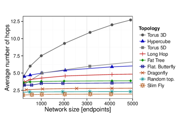
Figure 1: Comparison of the average number of hops (uniform traffic) in Slim Fly and other networks. Topologies are in balanced or close to balanced configurations (explained in Section III), allowing for highest global bandwidth.

Slim Fly enables us to construct cost-efficient full-bandwidth networks with over 100K endpoints with diameter two using readily available high radix routers (e.g., 64-port Black Widow [50] or Mellanox 108-port Director [4]). Larger networks with up to tens of millions of endpoints can be constructed with diameter three as discussed in Section II-A.

The main contributions of this work are:

• We design and analyze a new class of cost effective low-diameter network topologies called Slim Flies.

• We discuss and evaluate different deadlock-free minimal and adaptive routing strategies and we compare them to existing topologies and approaches.

• We show that, in contrast to the first intuition, Slim Fly, using fewer cables and routers, is more tolerant towards link failures than comparable Dragonflies.

• We show a physical layout for a datacenter or an HPC center network and a detailed cost and energy model.

• We provide a library of practical topologies with different degrees and network sizes that can readily be used to construct efficient Slim Fly networks. The link also contains the code of all simulations from Sections III-VI for reproducibility.

II Slim Fly Topologies

We now describe the main idea behind the design of Slim Fly. Symbols used in the paper are presented in Table I.

$N$	Number of endpoints in the whole network
$p$	Number of endpoints attached to a router (concentration)
$k^{\prime}$	Number of channels to other routers (network radix)
$k$	Router radix ($k=k^{\prime}+p$)
$N_{r}$	Number of all routers in the network
$D$	Network diameter

TABLE I: Symbols used in the paper

II-A Construction Optimality

The goal of our approach is to design an optimum or close-to-optimum topology that maximizes the number of endpoints $N$ for a given diameter $D$ and radix $k$ and maintains full global bandwidth. In order to formalize the notion of optimality we utilize the well-known concept of Moore Bound [47]. The Moore Bound (MB) determines the maximum number of vertices that a potential graph with a given $k$ and $D$ can have. We use the MB concept in our construction scheme and we define it to be the upper limit on the number of radix-$k$ routers that a network with a given diameter $D$ can contain. The Moore Bound of such a network is equal to $N_{r}=1+k^{\prime}\sum_{i=0}^{D-1}(k^{\prime}-1)^{i}$ [47], where $k^{\prime}=\lceil\frac{2k}{3}\rceil$ enables full global bandwidth for $D=2$ as we will show in Section II-B2.

MB is the upper bound on the number of routers $N_{r}$ and thus also endpoints $N$ in the network. For $D=2$, the maximum $N_{r}$ $\approx k^{\prime 2}$. Thus, an example network constructed using 108-port Mellanox Director switches would have nearly 200,000 endpoints (we discuss the selection of the concentration $p$ in Section II-B2). For $D=3$, $N_{r}$ is limited to $\approx k^{\prime 3}$, which would enable up to tens of millions of endpoints. Thus, we focus on graphs with diameter two and three for relevant constructions. To construct Slim Flies, we utilize graphs related to the well-known degree–diameter problem [47], which is to determine the largest graphs for a given $k^{\prime}$ and $D$.

II-B Diameter-2 Networks

An example diameter-2 graph, which maximizes the number of vertices per given $k^{\prime}$ and $D$, is the well-known Hoffman–Singleton graph [46] with 50 radix-7 vertices and 175 edges. In general, there exists no universal scheme for constructing such optimum or close-to-optimum graphs. For most $D$ and $k^{\prime}$ it is not known whether there exist optimal graphs, or how close one can get to the Moore Bound [46].

However, some of the introduced graphs are very close to the optimum. In order to develop a diameter-2 network we utilize a family of such graphs introduced by McKay, Miller, and Širán in [46] (we denote them as MMS graphs). We adopt MMS graphs and we design the Slim Fly topology (denoted as SF MMS) basing on them. The theory of MMS graphs is deeply rooted in the graph covering techniques and other related concepts [46]. For clarity, we present a simplified construction scheme (together with an intuitive example); additional details can be found in [46, 58, 35].

II-B1 Connecting Routers

The construction of SF MMS begins with finding a prime power $q$ such that $q=4w+\delta$, where $\delta\in\{-1,0,1\}$ and $w\in\mathbb{N}$. For such $q$ we generate an MMS graph with network radix $k^{\prime}=\frac{3q-\delta}{2}$ and number of vertices (routers) $N_{r}=2q^{2}$.

Step 1: Constructing Base Ring $\mathbb{Z}_{q}$

Let $\mathbb{Z}_{q}=\{0,1,...,q-1\}$ be a commutative ring with modulo addition and multiplication. We have to find a primitive element $\xi$ of $\mathbb{Z}_{q}$. $\xi$ is an element of $\mathbb{Z}_{q}$ that generates $\mathbb{Z}_{q}$: all non-zero elements of $\mathbb{Z}_{q}$ can be written as $\xi^{i}$ ($i\in\mathbb{N}$). In general, there exists no universal scheme for finding $\xi$ [45], however an exhaustive search is viable for smaller rings; all the SF MMS networks that we tested were constructed using this approach.

Step 2: Constructing Generator Sets $X$ and $X^{\prime}$

In the next step we utilize $\xi$ to construct two sets $X$ and $X^{\prime}$ called generators [35]. For $\delta=1$ we have $X=\{1,\xi^{2},...,\xi^{q-3}\}$ and $X^{\prime}=\{\xi,\xi^{3},...,\xi^{q-2}\}$ (consult [35] for other formulae). We will use both $X$ and $X^{\prime}$ while connecting routers.

Step 3: Constructing and Connecting Routers

The set of all routers is a Cartesian product: $\{0,1\}\times\mathbb{Z}_{q}\times\mathbb{Z}_{q}$. Routers are connected using the following equations [35]:

$$\mbox{router }(0,x,y)\mbox{ is connected to }(0,x,y^{\prime})\mbox{ iff }y-y^{\prime}\in X;$$ (1)

$$\mbox{router }(1,m,c)\mbox{ is connected to }(1,m,c^{\prime})\mbox{ iff }c-c^{\prime}\in X^{\prime};$$ (2)

$$\mbox{router }(0,x,y)\mbox{ is connected to }(1,m,c)\mbox{ iff }y=mx+c;$$ (3)

Intuitively, MMS graphs have highly symmetric internal structure: they consist of two subgraphs, each composed of the same number of identical subgroups of routers. The first subgraph is composed of routers $(0,x,y)$ while the other consists of routers $(1,m,c)$. An overview is presented in Figure 2. We will use this property while designing a physical layout for a datacenter or an HPC center in Section VI-A.

Figure 2: General structure of the MMS graph (§ II-B1).

(a) Connections between routers in each subgraph (§ II-B1, Eq. (1)-(2)). Note that respective groups have identical connection patterns.

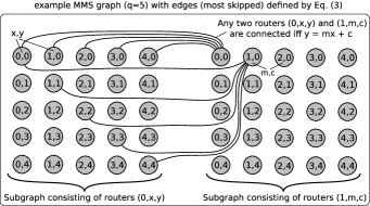
(b) Connections between two subgraphs (§ II-B1, Eq. (3)). For clarity we present only the edges originating at $(1,0,0)$ and $(1,1,0)$.

Figure 3: Connecting routers in an MMS graph ($q=5$). For clarity, we denote routers $(0,x,y)$ as $x,y$; and routers $(1,m,c)$ as $m,c$.

Example MMS Construction for $q=5$

We now construct an example MMS (the Hoffman-Singleton graph) to illustrate the presented scheme in practice. We select $q=5$, thus $\mathbb{Z}_{5}=\{0,1,2,3,4\}$ and the primitive element $\xi=2$. We can verify it easily by checking that: $1=\xi^{4}\;mod\;5=2^{4}\;mod\;5$, $2=2^{1}\;mod\;5$, $3=2^{3}\;mod\;5$, $4=2^{2}\;mod\;5$. The construction of generator sets is also straightforward: $X=\{1,2^{2},...,2^{5-3}\}=\{1,4\}$ and $X^{\prime}=\{2,2^{3},...,2^{5-2}\}=\{2,3\}$ (all operations are of course done modulo $q$).

The router set of our SF MMS is $\{0,1\}\times\mathbb{Z}_{5}\times\mathbb{Z}_{5}$. We apply Equation (1) to connect routers $(0,x,y)$. Then, we use Equation (2) for routers $(1,m,c)$. The results are shown in Figure 3a; for clarity, we denote routers $(0,x,y)$ as $x,y$; and routers $(1,m,c)$ as $m,c$. Finally, we apply Equation (3) to connect routers $(0,x,y)$ with $(1,m,c)$ (see Figure 3b).

II-B2 Attaching Endpoints

We now illustrate our formula for $p$ (concentration) that ensures full global bandwidth. The global bandwidth of a network is defined as the theoretical cumulative throughput if all processes simultaneously communicate with all other processes in a steady state. To maximize the global bandwidth of SF MMS, we first consider the network channel load (we model each full-duplex link with two channels, one in each direction): each router can reach $k^{\prime}$ routers in distance one and $N_{r}-k^{\prime}-1$ routers in distance two. The whole network has a total number of $k^{\prime}\cdot N_{r}$ channels. We define the channel load $l$ as the average number of routes (assuming minimal routing) that lead through each link of the network. We have $p$ endpoints per router and each router forwards messages to approximately $p\cdot N_{r}$ destinations from each local endpoint. We get a total average load per channel $l=\frac{(k^{\prime}+2\cdot(N_{r}-k^{\prime}-1))\cdot p^{2}N_{r}}{k^{\prime}N_{r}}=\frac{(2N_{r}-k^{\prime}-2)\cdot p^{2}}{k^{\prime}}$.

Each endpoint injects to approximately $N=pN_{r}$ destinations through its single uplink. A network is called balanced if each endpoint can inject at full capacity, i.e., $pN_{r}=[(2N_{r}-k^{\prime}-2)\cdot p^{2}]/k^{\prime}$. Thus, we pick the number of endpoints per router $p\approx\frac{k^{\prime}N_{r}}{2N_{r}-k^{\prime}-2}=\frac{N_{r}}{l}$ to achieve full global bandwidth. Finally, we get $p\approx k^{\prime}/(2-\frac{k^{\prime}}{N_{r}}-\frac{2}{N_{r}})\approx\left\lceil k^{\prime}/2\right\rceil$ which means that $\approx 67\%$ of each router’s ports connect to the network and $\approx 33\%$ of the ports connect to endpoints. An overview of the connections originating at a single router is presented in Figure 4.

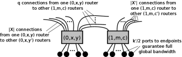
Figure 4: Connecting routers and endpoints in SF MMS.

(a) The MB and graphs with $D=2$ (§ II-B3).

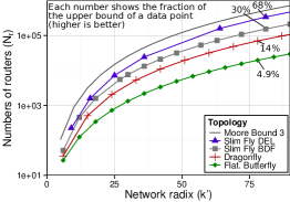
(b) The MB and graphs with $D=3$ (§ II-C).

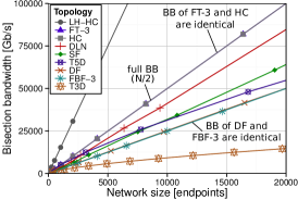
(c) Bisection bandwidth (BB) comparison (§ III-C).

Figure 5: Comparison of the Moore Bound (for diameter 2 and 3 constructions) and bisection bandwidth (we assume 10 Gb/s/link). For the Moore Bound comparison we skip networks which does not have constant diameter (random topologies, hypercube, and tori).

II-B3 Comparison to Optimality (the Moore Bound)

Figure 5a compares the distance between topologies with $D=2$ and the MB. We see that SF MMS is very close to the optimum. For $k^{\prime}=96$, MMS has 8,192 routers, which is only 12% worse than the upper bound (9,217). Other topologies (a Long Hop described in Section E-S-1 of [56], a two-stage fat tree, and a two-level Flattened Butterfly) are up to several orders of magnitude worse. Thus, in the paper we do not compare to these topologies, as they cannot be easily used to construct networks of practical size (e.g., a Long Hop with merely 50,000 endpoints requires routers with radix $\approx$340).

II-C Diameter 3 Networks

We present two classes of graphs that approach the MB for $D=3$. Bermond, Delorme and Fahri (BDF) graphs can be generated using a scheme described in [6]. They have $k^{\prime}=\frac{3(u+1)}{2}$ and $N_{r}=\frac{8}{27}k^{\prime 3}-\frac{4}{9}k^{\prime 2}+\frac{2}{3}k^{\prime}$ for a given odd prime power $u$. The second class are Delorme (DEL) graphs [24] characterized by $N_{r}=(v+1)^{2}(v^{2}+1)^{2}$ and $k^{\prime}=(v+1)^{2}$ for a given prime power $v$.

Figure 5b compares the number of routers in BDF and DEL graphs with two other networks that have $D=3$: Dragonfly and 3-level Flattened Butterfly. Dragonfly achieves only 14% (e.g. for $k^{\prime}=96$) of the maximum possible number of routers for a given $k^{\prime}$ and $D=3$; Flattened Butterfly is $\approx$3 times worse. Delorme and BDF graphs achieve, respectively, 68% and 30% of the Moore Bound.

II-C1 Constructing BDF graphs

The $*$ Product

Consider two graphs $G_{1}=(V_{1},E_{1})$ and $G_{2}=(V_{2},E_{2})$. Let $U$ be a set of arcs constructed from the edges of $G_{1}$ by taking an arbitrary orientation. Let $f_{(x,y)}$ be a one-to-one mapping from $V_{2}$ to itself, for any arc $(x,y)$ [6].

The $*$ product creates a new graph $G^{\prime}=(V^{\prime},E^{\prime})=G_{1}*G_{2}$. $V^{\prime}$ is a cartesian product $V_{1}\times V_{2}$. A vertex $(a_{1},a_{2})\in V^{\prime}$ is connected to $(b_{1},b_{2})\in V^{\prime}$ iff either $a_{1}=b_{1}\land\{a_{2},b_{2}\}\in E_{2}$, or $(a_{1},b_{1})\in U\land b_{2}=f_{(a_{1},b_{1})}(a_{2})$ [6].

Constructing Graph $P_{u}$

Assume $u$ is an odd prime power. We know that there exists a projective plane of order $u$ with a numbering of the points ($M_{i}$) and of the lines ($D_{j}$) [6] where $1\geq M_{i},D_{j}\leq u^{2}+u+1$ and $M_{i}\in D_{j}\Rightarrow M_{j}\in D_{i}$. We now construct a graph $P_{u}$ from the points of the projective plane. Two vertices $M_{i}$ and $M_{j}$ are connected iff $M_{j}\in D_{i}$. $P_{u}$ has a diameter of 2, degree $u+1$, and $u^{2}+u+1$ vertices [6].

Constructing the Final Graph $P_{u}*G_{k^{\prime}/3}$

We say that a graph $G=(V,E)$ has property $P^{*}$ iff it has a diameter of at most 2 and there exists an involution $f$ of $V$ such that $\forall_{v\in V}:\quad V=\{v\}\cup\{f(v)\}\cup\{f(\Gamma(v))\}\cup\{\Gamma(f(v))\}$ [6].

Let $k^{\prime}=\frac{3(u+1)}{2}$ and let $G_{k^{\prime}/3}$ be a graph satisfying property $P^{*}$ (see [6] for construction details). A graph $P_{u}*G_{k^{\prime}/3}$ has diameter 3, degree $k^{\prime}$, and $N_{r}=\frac{8}{27}k^{\prime 3}-\frac{4}{9}k^{\prime 2}+\frac{2}{3}k^{\prime}$.

In this work, we focus on MMS graphs because their scalability suffices for most large-scale networks having more than 100K endpoints. Analyses with the diameter three constructions show lower but similar results in terms of cost and performance benefits over other topologies since they approach the optimal structure.

III Slim Fly Structure Analysis

We now analyze the structure of SF MMS in terms of common metrics: network diameter, average distance, bisection bandwidth, and resiliency. We compare Slim Fly to the topologies presented in Table II. Most of them are established and well-known designs and we refer the reader to given references for more details. DLN are constructed from a ring topology by adding random edges identified by a number of routers and degree [42]. Long Hops are networks constructed from Cayley graphs using optimal error correcting codes [56] We utilize a variant of Long Hops that augments hypercubes (introduced in Section E-S-3 of [56]).

Topology parameters For high radix networks we select the concentration $p$ to enable balanced topology variants with full global bandwidth. Respective values of $p$, expressed as a function of radix $k$, are as follows: $p=\lfloor(k+1)/4\rfloor$ (DF), $p=\lfloor(k+3)/4\rfloor$ (FBF-3), $p=\lfloor\sqrt{k}\rfloor$ (DLN), $p=\lfloor k/2\rfloor$ (FT-3). For lower radix topologies (T3D, T5D, HC, LH-HC) we select $p=1$ following strategies from [1, 40, 39].

III-A Network Diameter

The structure of MMS graphs ensures that SF’s diameter is 2. The comparison to other topologies is illustrated in Table II. For LH-HC we report the values for generated topologies of size from $2^{8}$ to $2^{13}$ endpoints ($D$ increases as we add endpoints). Numbers for DLN come from [42]. SF offers the lowest diameter out of all compared topologies.

Topology	Symbol	Example System	Diameter
3-dimensional torus [3]	T3D	Cray Gemini [3]	$\lceil 3/2\sqrt[3]{N_{r}}\rceil$
5-dimensional torus [21]	T5D	IBM BlueGene/Q [20]	$\lceil 5/2\sqrt[5]{N_{r}}\rceil$
Hypercube [59]	HC	NASA Pleiades [59]	$\lceil\log_{2}N_{r}\rceil$
3-level fat tree [44]	FT-3	Tianhe-2 [27]	4
3-level Flat. Butterfly [40]	FBF-3	-	3
Dragonfly topologies [41]	DF	Cray Cascade [29]	3
Random topologies [42]	DLN	-	3–10
Long Hop topologies [56]	LH-HC	Infinetics Systems [56]	4–6
Slim Fly MMS	SF	-	2

TABLE II: Topologies compared in the paper, their diameters (§ III-A), and example existing HPC systems that use respective topologies.

III-B Average distance

The distance between any two endpoints in SF is always equal to or smaller than two hops. We compare SF to other topologies in Figure 1. The average distance is asymptotically approaching the network diameter for all considered topologies and is lowest for SF for all analyzed network sizes.

III-C Bisection Bandwidth

Figure 5c presents the bisection bandwidth (BB) of compared topologies. For SF and DLN we approximate the bisection bandwidth using the METIS [37] partitioner. Bisection bandwidths for other topologies can be derived analytically and are equal to: $\lfloor\frac{N}{2}\rfloor$ (HC and FT-3), $\lfloor\frac{2N}{k^{\prime}}\rfloor$ (tori), and $\lfloor\frac{N+2p^{2}-1}{4}\rfloor\approx\lfloor\frac{N}{4}\rfloor$ (DF and FBF-3)  [41, 40, 44, 23, 56]. LH-HC has the bandwidth of $\lfloor\frac{3N}{2}\rfloor$ as it was designed specifically to increase bisection bandwidth. SF offers higher bandwidth than DF, FBF-3, T3D, and T5D.

III-D Resiliency

We compare SF to other topologies using three different resiliency metrics. To prevent deadlocks in case of link failures, one may utilize Deadlock-Free Single Source Shortest Path (DFSSSP) routing [26] (see Section IV-D for details).

III-D1 Disconnection Metrics

We first study how many random links have to be removed before a network becomes disconnected. We simulate random failures of cables in 5% increments with enough samples to guarantee a 95% confidence interval of width 2. Table III illustrates the results of the analysis. The three most resilient topologies are SF, DLN, and FBF-3. Interestingly, random topologies, all with diameter three in our examples, are very resilient, and one can remove up to 75% of the links before the network is disconnected. This can be explained with the emergence of the giant component known from random graph theory [19]. FBF-3 is also resilient thanks to high path diversity. DF, also diameter three, is less resilient due to its structure, where a failure in a global link can be disruptive. A similar argumentation applies to FT-3. For torus networks, the resilience level decreases as we increase $N$. This is due to a fixed radix that makes it easier to disconnect bigger networks. Finally, the resilience level of both HC and LH-HC does not change with $N$. The radix of both networks increases together with $N$, which prevents the resilience level from decreasing as in tori. Still, the rate of this increase is too slow to enable gains in resilience as in high radix topologies.

$\approx N$	T3D	T5D	HC	LH-HC	FT-3	DF	FBF-3	DLN	SF
256	25%	50%	40%	55%	-	45%	50%	-	45%
512	-	-	40%	55%	35%	-	55%	60%	60%
1024	15%	40%	40%	55%	40%	50%	60%	-	-
2048	10%	-	40%	55%	40%	55%	65%	65%	65%
4096	5%	40%	45%	55%	55%	60%	70%	70%	70%
8192	5%	35%	45%	55%	60%	65%	-	75%	75%

TABLE III: Disconnection Resiliency (§ III-D1): the maximum number of cables that can be removed before the network is disconnected. Missing values indicate the inadequacy of a balanced topology variant for a given $N$.

SF, the only topology with $D=2$, is highly resilient as its structure provides high path diversity. As we will show in Section VI-A, SF has a modular layout similar to DF. However, instead of one link between groups of routers there are $2q$ such links, which dampens the results of a global link failure.

III-D2 Increase in Diameter

Similarly to Koibuchi et al. [42], we also characterize the resiliency by the increase in diameter while removing links randomly. For our analysis, we make the (arbitrary) assumption that an increase of up to two in diameter can be tolerated. The relative results are similar to the ones obtained for disconnection metrics. The only major difference is that non-constant diameter topologies such as tori are now rather resilient to faults because random failures are unlikely to lie on a critical path. For a network size $N=2^{13}$, SF can withstand up to 40% link failures before the diameter grows beyond four. The resilience of SF is slightly worse than DLN (tolerates up to 60% link failures), comparable to tori, and significantly better than DF (withstands 25% link failures).

III-D3 Increase in Average Path Length

While the diameter may be important for certain latency-critical applications, other applications benefit from a short average path length (which may also increase the effective global bandwidth). Thus, we also investigate the resiliency of the average path length of the topologies. We assume that an increase of one hop in the average distance between two nodes can be tolerated. Again, this is an arbitrary value for the purpose of comparison. The results follow a similar pattern as for the diameter metrics. Tori survive up to 55% link failures. DLN is most resilient and can sustain up to 60% link failures for a network with $N=2^{13}$. DF withstands up to 45% of link crashes. SF is again highly resilient and it tolerates up to 55% link failures.

IV Routing

We now discuss minimal and non–minimal routing for SF and we present a UGAL–L (global adaptive routing using local information) algorithm suited for SF together with the comparison to UGAL–G as defined in [51]. We also show how to guarantee deadlock-freedom in SF. We consider routing packets from a source endpoint $s$ attached to a router $R_{s}$ to a destination endpoint $d$ connected to a router $R_{d}$.

IV-A Minimal Static Routing

In minimal (MIN) routing in SF a packet is routed either directly (if $R_{s}$ is connected to $R_{d}$) or using two hops if the distance between $R_{s}$ and $R_{d}$ is two. Such minimal routing can easily be implemented with current statically routed networking technologies such as InfiniBand or Ethernet.

IV-B Valiant Random Routing

The Valiant Random Routing (VAL) algorithm [57] can be used for Slim Fly to load–balance adversarial traffic scenarios for which minimum routing is inefficient. To route a packet, the protocol first randomly selects a router $R_{r}$ different from $R_{s}$ and $R_{d}$. The packet is then routed along two minimal paths: from $R_{s}$ to $R_{r}$, and from $R_{r}$ to $R_{d}$. Paths generated by VAL may consist of 2, 3, or 4 hops, depending on whether routers $R_{s}$, $R_{r}$, and $R_{d}$ are directly connected. One may also impose a constraint on a selected random path so that it contains at most 3 hops. However, our simulations indicate that this results in higher average packet latency because it limits the number of available paths (we discuss our simulation infrastructure and methodology in detail in Section V).

IV-C Non–minimal Adaptive Routing

The Universal Globally–Adaptive Load–balanced (UGAL) algorithm [51] selects either a minimum or a VAL–generated path for a packet basing on hop distance and sizes of queues between two endpoints. For SF we investigate two variants.

IV-C1 Global UGAL Version (UGAL–G)

UGAL–G has access to the sizes of all router queues in the network. For each injected packet it generates a set of random VAL paths, compares them with the MIN path, and selects a path with the smallest sum of output router queues. Our simulations indicate that the choice of 4 paths provides the best average packet latency. UGAL–G approximates the ideal implementation of UGAL routing and thus provides a good way to evaluate the quality of the local version.

IV-C2 Local UGAL Version (UGAL–L)

UGAL–L can only access the local output queues at each router. To route a packet, it first generates a set of VAL paths and computes the MIN path. Then, it multiplies the length of each path (in hops) by the local output queue length, and picks the one with the lowest result. The number of generated random paths influences the simulation results. We compared implementations using between 2 and 10 random selections and we find empirically that selecting 4 results in lower overall latency.

(a) Random traffic (§ V-A).

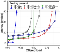
(b) Bit reverse traffic (§ V-B).

(c) Shift traffic (§ V-B).

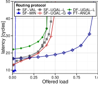
(d) Worst-case traffic (§ V-C).

Figure 6: Performance comparison of SF, DF, and FT-3. We use different protocols in the Slim Fly analysis: minimum static routing (SF-MIN), Valiant (SF-VAL), UGAL-L (SF-UGAL-L), UGAL-G (SF-UGAL-G). For DF and FT-3 we use Dragonfly UGAL-L (DF-UGAL-L) and Adaptive Nearest Common Ancestor (FT-ANCA), respectively. We use the buffer size of 64 flit entries.

IV-D Deadlock-Freedom

We use a strategy similar to the one introduced by Gopal [34, 28]. We use two virtual channels (VC0 and VC1) for minimal routing. Assume we send a packet from router $R_{a}$ to $R_{b}$. If the routers are directly connected, then the packet is routed using VC0. If the path consists of two hops, then the we use VC0 and VC1 for the first and the second hop, respectively. We illustrate an example application of our strategy in Figure 7. Since the maximum distance in the network is two, only one turn can be taken on the path and the number of needed VCs is thus no more than two.

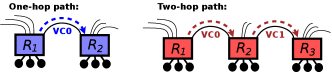
Figure 7: Virtual channels in Slim Fly.

For adaptive routing, we use four VCs (because of the maximum number of turns with distance four). Here, we simply generalize the scheme above and, for an $n$-hop path between $R_{a}$ to $R_{b}$, we use a VC $k$ ($0\leq k<n$) on a hop $k$.

To avoid deadlocks in minimum routing one can also use a generic deadlock-avoidance technique based on automatic VC assignment to break cycles in the channel dependency graph [30]. We tested the DFSSSP scheme implemented in the Open Fabrics Enterprise Edition (OFED) [26] which is available for generic InfiniBand networks. OFED DFSSSP consistently needed three VCs to route all SF networks. We also compared this number to random DLN networks [42], which needed between 8 and 15 VLs for network sizes of 338 endpoints and 1,682 endpoints, respectively.

V Performance

In this section we evaluate the performance of MIN, VAL, UGAL–L, and UGAL–G routing algorithms. We take into consideration various traffic scenarios that represent the most important HPC workloads. First, we test uniform random traffic for graph computations, sparse linear algebra solvers, and adaptive mesh refinement methods [60]. Second, we analyze shift and permutation traffic patterns (bit complement, bit reversal, shuffle) that represent some stencil workloads and collectives such as all-to-all or all-gather [60]. Finally, we evaluate a worst–case pattern designed specially for SF to test adversarial workloads.

We conduct cycle-based simulations using packets that are injected with a Bernoulli process and input-queued routers. Before any measurements are taken, the simulator is warmed up under load in order to reach steady-state. We use the strategy in [41] and utilize single flow control unit (flit) packets to prevent the influence of flow control issues (wormhole routing, virtual cut-through flow control) on the routing schemes. Three virtual channels are used for each simulation. Total buffering/port is 64 flit entries; we also simulated other buffer sizes (8, 16, 32, 128, 256). Router delay for credit processing is 2 cycles. Delays for channel latency, switch allocation, VC allocation, and processing in a crossbar are 1 cycle each. Speedup of the internals of the routers over the channel transmission rate is 2. Input/output speedups are set to 1.

We compare topologies with full global bandwidth in Figure 6 and Sections V-A, V-B, V-C, V-D. We also provide results for oversubscribed SF in Section V-E. Due to space constraints and for clarity of plots we compare SF to two established topologies: Dragonfly (representing low-latency state-of-the-art networks) and fat tree (representing topologies offering high bisection-bandwidth). We select established and highly-optimized routing protocols for DF and FT-3: UGAL-L [41] and the Adaptive Nearest Common Ancestor protocol (ANCA) [33], respectively. We use FT-3 instead of Long Hop since there is no proposed routing scheme for LH-HC [56] and designing such a protocol is outside the scope of our paper. We present the results for $N$ $\approx$ 10K. Simulations of networks with $N\approx$ 1K, 2K, and 5K give similar results (latency varies by at most 10% compared to networks with 10K nodes). The parameters for DF are as follows: $k=27$, $p=7$, $N_{r}=1,386$, $N=9,702$. FT-3 has $k=44$, $p=22$, $N_{r}=1,452$, $N=10,648$. Finally, SF has $k=44$, $p=15$, $N_{r}=722$, $N=10,830$. To enable fair performance comparison we simulate balanced variants of networks with full global bandwidth. Thus, they do not have exactly the same $N$; we chose networks that vary by at most 10% in $N$. We also investigated variants with exactly 10K endpoints that are either under- or oversubscribed; the results follow similar performance patterns. SF outperforms other topologies in terms of latency and offers comparable bandwidth.

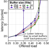
(a) Various buffer sizes.

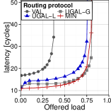
(b) Random traffic, $p=16$.

(c) Worst-case traffic, $p=16$.

(d) Random traffic, $p=18$.

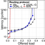
(e) Worst-case traffic, $p=18$.

Figure 8: Performance analysis of SF. In Figure 8a we illustrate the influence of the router input buffer size on the performance of Slim Fly for the worst-case traffic. Figures 8b - 8e present the results of the simulations of different oversubscribed variants of Slim Fly .

V-A Random Traffic for Irregular Workloads

In a random scenario each endpoint randomly selects the destination for an injected packet. The results are presented in Figure 6a. As expected, UGAL-G and MIN achieve the best performance. VAL takes longer paths on average and saturates at less than 50% of the injection rate because it doubles the pressure on all links. UGAL-L performs reasonably well (saturation at 80% of the injection rate) but packets take some detours due to transient local backpressure. This slightly decreases the overall performance at medium load but converges towards full bandwidth for high load (the difference is around 5% for the highest injection rate; this effect, described in [36], is much less visible in SF than in DF thanks to SF’s lower diameter resulting in fewer queues that can congest). As expected from Figure 5c, DF offers lower bandwidth while the bandwidth of FT-3 is slightly higher than SF. Finally, SF has the lowest latency due to its lower $D$ than in DF and FT-3.

V-B Bit Permutation and Shift Traffic for Collective Operations

We use several bit permutation scenarios to fully evaluate the performance of SF. As $N$ has to be a power of two we artificially prevent some endpoints from sending and receiving packets for the purpose of this evaluation. The number of endpoints that are active is 8,192 (power of two closest to the original size of the networks). We denote $b$ as the number of bits in the endpoint address, $s_{i}$ as the $i$th bit of the source endpoint address, and $d_{j}$ as the $j$th bit of the destination endpoint address. We simulate the shuffle ($d_{i}=s_{i-1~{}mod~{}b}$), bit reversal ($d_{i}=s_{b-i-1}$), and bit complement ($d_{i}=\neg s_{i}$) traffic pattern. We also evaluate a shift pattern in which, for source endpoint $s$, destination $d$ is (with identical probabilities of $\frac{1}{2}$) equal to either $d=(s\;mod\;\frac{N}{2})+\frac{N}{2}$ or $d=(s\;mod\;\frac{N}{2})$. We present the results in Figures 6b–6c (due to space constraints we skip bit reverse/complement). The bandwidth of FT-3, higher than UGAL–L and only slightly better than UGAL–G, indicates that the local decisions made by UGAL-L miss some opportunity for traffic balancing. As expected, SF offers slightly higher bandwidth and has lower latency than DF.

V-C Worst–Case Traffic for Adversarial Workloads

We now describe the worst-case traffic pattern for minimal deterministic routing on Slim Fly networks. For this, we consider only traffic patterns that do not overload endpoints. The scheme is shown in Figure 9. The worst-case pattern for a Slim Fly network is when all $p$ endpoints attached to routers $R_{1},...,R_{a}$ send and receive from all endpoints at router $R_{x}$ and the shortest path is of length two and leads via router $R_{y}$. In addition, all $p$ endpoints at routers $R_{1},...,R_{b}$ send and receive from all endpoints at router $R_{y}$ and the shortest path leads through router $R_{x}$. This puts a maximum load on the link between routers $R_{x}$ and $R_{y}$. We generate this pattern by selecting a link between $R_{x}$ and $R_{y}$ and choosing routers $R_{1},...,R_{a}$ and $R_{1},...,R_{b}$ according to the description above until all possibilities are exhausted. For DF we use a worst-case traffic described in Section 4.2 in [41]. In FT-3 we utilize a pattern where every packet traverses core (highest-level) switches in the topology.

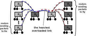
Figure 9: Illustration of the worst–case scenario for Slim Fly .

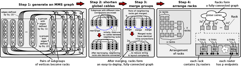
Figure 10: An MMS graph and the corresponding datacenter layout.

Figure 6d shows the simulation results of adversarial traffic. MIN routing is limited to $\frac{1}{p+1}$ throughput in the worst-case. VAL and UGAL-L can disperse the traffic across multiple channels and can support up to 40% (VAL) and 45% (UGAL-L) offered load, providing slightly higher bandwidth than DF. As we use the balanced full-bandwidth variant of FT-3, it achieves higher bandwidth than both DF and SF.

V-D Study of Buffer Sizes

We also analyze how the size of input router buffers affects the performance of SF. We present the results for the worst-case traffic in Figure 8a (other scenarios follow similar performance patterns). Smaller sizes result in lower latency (due to stiffer backpressure propagation), while bigger buffers enable higher bandwidth.

V-E Oversubscribing Slim Fly Networks

Oversubscribing the number of endpoints per router increases the flexibility of port count and cost of SF. We define an oversubscribed network as a network which cannot achieve full global bandwidth, cf. Section II-B2.

Figures 8b–8e show the latency and bandwidth of different oversubscribed SF networks with network radix $k^{\prime}=29$. In its full-bandwidth configuration ($p=15$) it supports 10,830 endpoints. We investigate six different oversubscribed networks with concentration 16–21 connecting from 11,552 up to 15,162 endpoints, respectively. We present the results for $p=16$ and $p=18$, other cases follow similar performance patterns. According to [22], we define the accepted bandwidth as the offered load of random uniform traffic which saturates the network. The full-bandwidth SF can accept up to 87,5% of the traffic. The SF with $p=16$ and $p=18$ accept up to 80% and 75% of the offered traffic, respectively. The bandwidth for the worst-case traffic behaves similarly. This study illustrates the flexibility of the SF design that allows for adding new endpoints while preserving high bandwidth and low latency.

We conclude that SF can deliver lower latency and in most cases comparable bandwidth in comparison to other topologies. As we will show in Section VI, by lowering the diameter Slim Fly offers comparable bandwidth and lower latency for lower price and energy consumption per endpoint.

VI Cost and Power Comparison

We now proceed to provide cost and power comparison of SF with other topologies. We also discuss the engineering constraints and partitioning of SF into groups of routers.

VI-A Physical Layout

One engineering challenge for a low-diameter network is how to arrange it in an HPC center or a datacenter with minimal cabling costs. We now describe a possible physical arrangement of SF. We focus on making SF deployable (with symmetric partitioning/modularity). Remaining issues such as incorporating power supply units can be solved with well-known strategies used for other modular networks (e.g., DF).

We arrange the routers and their attached endpoints into racks with an equal number of cables connecting the racks. We partition Slim Fly basing on the modular structure of the underlying MMS graph (see Section II-B, Figure 2, and the left side of Figure 10 (Step 1)). The MMS modular design enables several different ways of easy partitioning. We focus here on the most intuitive one, valid for prime $q$: two corresponding subgroups of vertices (one consisting of routers $(0,x,y)$, the other consisting of routers $(1,m,c)$) form one rack. The $q$ connections between these two subgroups plus their original intra-group edges defined by Equations (1) and (2) become intra-group cables of a single rack.

We illustrate how a datacenter layout originates from an MMS graph in Figure 10. First, in order to limit the cost, we rearrange subgroups of routers so that the length of global cables is reduced (Step 2). Note that, from the point of view of the MMS structure, we simply utilize the fact that no edges connect subgroups of routers $(0,x,y)$ with one another (the same holds for routers $(1,m,c)$).

Second, the neighboring groups of routers $(0,x,y)$ and $(1,m,c)$ are merged; newly-created groups of vertices form racks (Figure 10, Step 3). Note that, as we always merge one group of routers $(0,x,y)$ with another group of routers $(1,m,c)$, after this step each rack has the same pattern of intra-group cables. In addition, the whole datacenter can now be viewed as a fully-connected graph of identical racks, with $2q$ inter-connections between every pair of racks. Such a design facilitates the wiring and datacenter deployment.

The final layout is illustrated in Step 4 in Fig. 10. We place the racks as a square (or a rectangle close to a square) where $x$ and $y$ are the numbers of racks along the corresponding dimensions. If the number of racks $N_{rck}$ is not divisible by any $x$ and $y$, then we find $z$ such that $N_{rck}=x\cdot y+z$ and we place remaining $z$ racks at an arbitrary side.

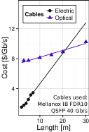
(a) Cable cost model.

(b) Routers cost model

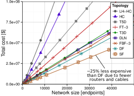
(c) Total cost of the network.

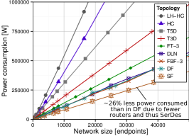
(d) Total power consumed by the network.

Figure 11: The details of the cost & power model and the comparison of Slim Fly to other topologies (cables: Mellanox InfiniBand (IB) FDR10 40Gb/s QSFP, routers: Mellanox IB FDR10).

(a) Cable cost model.

(b) Routers cost model

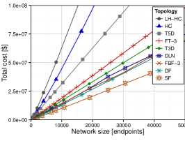
(c) Total cost of the network.

(d) Total power consumed by the network.

Figure 12: The details of the cost & power model and the comparison of Slim Fly to other topologies (cables: Elpeus Ethernet 10Gb/s SFP+, routers: Mellanox IB FDR10).

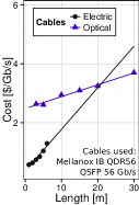
(a) Cable cost model.

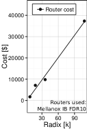
(b) Routers cost model

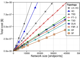
(c) Total cost of the network.

(d) Total power consumed by the network.

Figure 13: The details of the cost & power model and the comparison of Slim Fly to other topologies (cables: Mellanox InfiniBand (IB) QDR56 56Gb/s QSFP, routers: Mellanox IB FDR10).

As an example, consider an SF MMS network with $q=19$, consisting of 10,830 endpoints, with router radix $k^{\prime}=29$, concentration $p\approx\left\lceil k^{\prime}/2\right\rceil=15$ and $k=k^{\prime}+p=44$. For this network, we have $q=19$ racks, each containing 38 routers (570 endpoints), and 38 global channels to every other group. A different layout would allow for $q=39$ racks with 19 routers and 285 endpoints in each rack.

VI-A1 Slim Fly Layout vs. Dragonfly Layout

The final layout of SF is similar to that of DF: both form a 2-level hierarchy consisting of routers and groups of routers. We propose such construction scheme to facilitate the reasoning about SF. There are still some differences between SF and DF that ensure lower diameter/higher resiliency in SF:

• Routers inside each group in DF constitute fully-connected graphs. Routers inside groups in SF are not necessarily fully-connected.

• In DF, every router is connected to all $a-1$ remaining local routers in a group; in SF every router is connected to $\frac{a-\delta}{2}+1$ other local routers, which means that there are $\approx$50% fewer cables in a SF router group than in a DF router group.

• In DF, there is one inter-group cable connecting two groups. In SF, two groups are connected using $2q$ cables.

• A balanced SF has higher concentration ($p\approx 33\%k$) than a balanced same-size DF ($p\approx 25\%k$). This results in higher endpoint density and $\approx$25% fewer routers/racks in SF.

VI-B Cost Model

We now describe a cost model (similar to the model used in [40]) that includes the cost of routers and interconnection cables, which usually constitute the vast majority of the overall network costs [40]. We assume that routers together with endpoints are grouped in racks of size $1\times 1\times 2$ meters. Local (intra-rack) links are electric while global (inter-rack) channels are optic. Routers are placed on top of racks. The maximum Manhattan distance between two routers in a rack is $\approx$2m and the minimum is 5-10cm, thus on average intra-rack cables are 1m long. The distance between two racks is also calculated using the Manhattan metrics. Following [40], we add 2 meters of cable overhead for each global link. Racks are arranged in a shape close to a square as presented in Section VI-A.

VI-B1 Cables

To estimate the cost of network cables we use data bandwidth as a function of distance (in meters). We apply linear regression to today’s pricing data to get the cost functions. We use Mellanox InfiniBand (IB) FDR10 40Gb/s QSFP cables. Cost of electrical cables can be estimated as $f(x)=0.4079x+0.5771$ [$/Gb/s], while for optical fiber channels we have $f(x)=0.0919x+2.7452$ [$/Gb/s]. Figure 13a shows the model. Other cables that we considered are Mellanox IB QDR 56Gb/s QSFP, Mellanox Ethernet 40Gb/s QSFP, Mellanox Ethernet 10Gb/s SFP+, and Elpeus Ethernet 10Gb/s SFP+. They result in similar cost patterns (final relative cost differences between topologies vary by $\approx$1-2%; see Figure 12 and 13).

VI-B2 Routers

We also provide a function to calculate router cost basing on state of the art Mellanox IB FDR10 routers. We assume router cost to be a linear function of the radix because the router chip often has a rather constant price which is mainly determined by the development costs [41] while the SerDes are often the most expensive part of a router. We use linear regression to calculate the fit ($f(k)=350.4k-892.3$ [$]) and we show the model in Figure 13b. Other tested routers are Mellanox Ethernet 10/40Gb, they again only negligibly impact the relative cost differences between topologies ($\approx$1% difference between SF and DF).

VI-B3 Models of Remaining Network Topologies

Tori

We model T3D and T5D as cuboids and hyper cuboids, respectively. Following [41] we assume that tori have folded design that do not require optical links.

Hypercube and Long Hop

In HC and LH-HC, we use electric cables for intra- and fiber cables for inter-rack connections. Each router connects to a single router in each dimension. In LH-HC routers have additional $L$ ports to other routers as specified in Section E-S-3 of [56].

Fat tree

FT-3 has 3 layers with the sum of $5p^{2}$ routers that are installed in a central row in the network. Core routers are connected to aggregation routers with $2p^{3}$ optical cables. Each aggregation router is connected to $p$ edge routers giving a total of further $2p^{3}$ fiber channels. We estimate average cable length between routers to be 1m. Finally, the number of endpoints and the cables connecting them to routers is also $2p^{3}$; we assume that links shorter than 20 meters are electrical. $p^{2}$ endpoints form a single group (pod).

Flattened butterfly

We arrange routers and groups in FBF-3 as in [40]. There are $p$ routers in every group (rack) and $p^{2}$ groups forming an ideal square. Each group is fully connected ($\frac{p(p-1)}{2}$ electric channels) and there are $p$ fiber links between every two groups in the same row or column of racks.

Dragonfly and Random Networks

We use the balanced DF [41] ($a=2p=2h$). $a$ is the number of routers in a group and $h$ is the number of fiber cables connected to each router. There are $g=a\cdot h+1$ fully connected groups of routers, each having $\frac{a(a-1)}{2}$ electric cables. Groups form a clique with the total of $\frac{g(g-1)}{2}$ fiber cables [41]. DLN have groups with the same size ($a$), but cables are placed randomly.

	Low-radix topologies				High-radix topologies
Topology	T3D	T5D	HC	LH-HC	FT-3	DLN	FBF-3	DF	FT-3	DLN	FBF-3	DF	DF	SF
Endpoints ($N$)	10,648	10,368	8,192	8,192	19,876	40,200	20,736	58,806	10,718	9,702	10,000	9,702	10,890	10,830
Routers ($N_{r}$)	10,648	10,368	8,192	8,192	2,311	4,020	1,728	5,346	1,531	1,386	1,000	1,386	990	722
Radix ($k$)	7	11	14	19	43	43	43	43	35	28	33	27	43	43
Electric cables	31,900	50,688	32,768	53,248	19,414	32,488	9,504	56,133	7,350	6,837	4,500	9,009	6,885	6,669
Fiber cables	0	0	12,288	12,288	40,215	33,842	20,736	29,524	24,806	7,716	10,000	4,900	1,012	6,869
Cost per node [$]	1,682	3,176	4,631	6,481	2,346	1,743	1,570	1,438	2,315	1,566	1,535	1,342	1,365	1,033
Power per node [W]	19.6	30.8	39.2	53.2	14.0	12.04	10.8	10.9	14.0	11.2	10.8	10.8	10.9	8.02

TABLE IV: Cost and power comparison between a Slim Fly ($N=10830,k=43$) and other networks (§ VI-B4 and § VI-C). We select low-radix networks with $N$ comparable to that of Slim Fly. $N$ cannot be identical due to the limited number of existing network configurations. For high-radix topologies, we select comparable $N$ and we also compare to topologies with fixed radix $k$. We also construct and analyze one additional variant of a DF that has both comparable $N$ and identical $k$ as the analyzed SF. Each of these groups of topologies is indicated with a bolded parameter.

VI-B4 Discussion of the Results

Figure 13c presents the total cost of balanced networks. A detailed case-study showing cost per endpoint for an SF with $\approx$10K endpoints and radix $43$ can be found in Table IV. Here, we first compare SF to low-radix topologies (T3D, T5D, HC, LH-HC) with comparable network size $N$. $N$ cannot be identical for each topology due to the limited number of networks in their balanced configurations. We use tori with size close to that of SF (1-4% of difference). However, a small number of HC and LH-HC configurations forced us to use $N=8,192$ for these topologies. We additionally constructed hybrid hypercubes and Long Hops that consist of excessive routers and endpoints and are thus identical in size to SF; the cost results vary by only $\approx$1%. LH-HC is more expensive than HC because it uses additional links to increase bisection bandwidth. SF is significantly more cost-effective than low-radix networks as it uses fewer routers and cables.

Next, we present the results for balanced high-radix networks (FT-3, DLN, FBF-3, DF). We first compare to topologies that have similar $N$ (at most 10% of difference). Then, we select networks with the same radix $k$ as the analyzed SF. We also compare to one additional variant of a DF that has both comparable $N$ and identical $k$ as the analyzed SF. Such a construction is possible for DF because it has flexible structure based on three parameters $a$, $h$, and $p$ that can have any values. We perform an exhaustive search over the space of all Dragonflies that satisfy the condition $a\geq 2h$ and $p\geq h$. This condition ensures full utilization of global channels (see Section 3.1 in [41] for details). We select a DF that has $k=43$ and whose $N$ is closest to that of the analyzed SF. In all cases, SF is $\approx$25% more cost-effective than DF, and almost 30%, 40%, and 50% less expensive than FBF-3, DLN, and FT-3. The difference between SF and other topologies is achieved by the reduction in the number of needed routers and cables and the today’s commodization of fiber optics. For example, for a network with $k=43$ and $N\approx 10,000$, DF uses 990 routers while SF utilizes only 722 routers. However, DF uses fewer global cables than SF; thus, we expect that further commodization of optical cables will make the relative benefit of SF even bigger in the future.

VI-C Energy Model

Energy consumption of interconnects can constitute 50% of the overall energy usage of a computing center [2]. We now show that SF also offers substantial advantages in terms of such operational costs. Following [2] we assume that each router port has 4 lanes and there is one SerDes per lane consuming $\approx 0.7$ watts. We compare SF to other topologies using identical parameters as in the cost model. We present the results in Figure 13d and in Table IV. In general, SF is over 25% more energy-efficient than DF, FBF-3, and DLN. The power consumption in SF is lower than in other topologies thanks to the lower number of routers and thus SerDes.

VII Discussion

We demonstrated the Slim Fly topology which allows the construction of low-latency, full-bandwidth, and resilient networks at a lower cost than existing topologies.

VII-A Using Existing Routers

Network architects often need to adjust to existing routers with a given radix. As the construction of SF is based on powers of primes $q$, network radices $k^{\prime}$ (and thus router radices $k$) cannot have any arbitrary values for a simple construction. We now illustrate solutions to this issue.

First, the number of balanced SF constructions is significant. For network sizes up to 20,000, there are 11 balanced SF variants with full global bandwidth; DF offers only 8 such designs. Many of these variants can be directly constructed using readily available Mellanox routers with 18, 36, or 108 ports. Furthermore, the possibility of applying oversubscription of $p$ with negligible effect on network overall latency (see Section V-E) adds even more flexibility to the construction of network architectures based on SF.

Another option is to add random channels to utilize empty ports of routers with radix $>k$ (using strategies presented in [52, 42]). This would additionally improve the latency and bandwidth of such SF variants [52, 42]. For example, to construct a SF ($k=43$, $N=10830$) with 48-port routers (cf., Aries [29]), one could attach either five more endpoints or five random cables per router. In order to minimize costs, one could also limit the random connections to intra-rack copper links. We leave this analysis for future research.

VII-B Constructing Dragonfly-type Networks

An interesting option is to use SF to implement groups (higher-radix logical routers) of a DF or to connect multiple groups of a DF topology. This could decrease the costs in comparison to the currently used DF topologies [29, 41].

VII-C Adding New Endpoints Incrementally

SF can seamlessly handle incremental changes in the number of endpoints in computing centers. As we illustrated in the evaluation, the performance of SF is oblivious to relatively small oversubscription of $p$ and can still perform well when $p>\lceil k^{\prime}/2\rceil$. It leaves a lot of flexibility for adding new endpoints incrementally. For example, a network with 10,830 endpoints can be extended by $\approx$1500 endpoints before the performance drops by more than 10%. To achieve this, some ports in routers can be left empty and new endpoints would be added with time according to the needs. This strategy is used in today’s Cray computing systems [29].

VIII Related Work

Related topologies are summarized in Section III. The main benefits over traditional networks such as fat tree [44], and tori [23] are the significantly lower cost, energy consumption, and latency. The advantages over state-of-the-art topologies such as Flattened Butterfly [40] and Dragonfly [41] are higher bandwidth, lower latency, in most cases higher resiliency, and lower (by $\approx$25-30%) cost and energy consumption. The performance improvements are particularly important for data intense irregular workloads [54], such as graph processing [8, 17, 32, 53, 16, 14, 10, 11, 18, 15, 12] or others [49, 9, 31, 38, 7, 25], deep learning [5], or irregular matrix computations [43, 13]. In fact, Slim Fly networks are related to those topologies in that they minimize the diameter and reduce the number of routers while requiring longer fiber cables. In comparison to random networks, SF does not rely on a random construction for low diameter but starts from the lowest possible diameter. As discussed in Section VII-A, the ideas of random shortcut topologies can be combined with Slim Flies.

Jiang et al. [36] propose indirect adaptive routing algorithms for Dragonfly networks to balance the traffic over the global links. Since the Slim Fly topology is homogeneous, it does not have isolated “global links” that could be overloaded and backpressure is quickly propagated due to the low diameter. One can use similar ideas to discover congestion in the second hop to make better routing decisions for Slim Fly.

IX Conclusion

Interconnection networks constitute a significant part of the overall datacenter and HPC center construction and maintenance cost [2]. Thus, reducing the cost and energy consumption of interconnects is an increasingly important task for the networking community.

We propose a new class of topologies called Slim Fly networks to implement large datacenter and HPC network architectures. For this, we utilize a notion that lowering the network diameter reduces the amount of expensive network resources (cables, routers) used by packets traversing the network while maintaining high bandwidth. We define it as an optimization problem and we optimize towards the Moore Bound. We then propose several techniques for designing optimal networks. We adopt a family of MMS graphs, which approach the Moore Bound for $D=2$, and we design Slim Fly basing on them.

The Slim Fly architecture follows the technology trends towards high-radix routers and cost-effective fiber optics. Under the current technology constraints, we achieve a 25% cost and power benefit over Dragonfly. We expect that further commodization of fiber optics will lead to more cost-effective connections and further improvements in silicon process technology will lead to higher-radix routers. Both will make the relative benefit of Slim Fly even bigger in the future.

Our proposed routing strategies work well under bit permutation and worst-case traffic patterns and asymptotically achieve high bandwidth for random traffic. Thanks to the modular structure similar to Dragonfly, Slim Fly can be more easily deployed than other topologies such as random networks.

Theoretical analyses show that Slim Fly is more resilient to link failures than Dragonfly and approaches highly resilient constructions such as random topologies. This counter-intuitive result (since the topology utilizes less links and achieves a smaller diameter) can be explained by the structure of the graph which has the properties of an expander graph [48].

Finally, the introduced approach for optimizing networks using the Moore Bound can be extended for higher-diameter networks which, while providing slightly higher latency, could establish scalable structures allowing for millions of endpoints. We believe that our general approach, based on formulating engineering problems in terms of mathematical optimization, can effectively tackle other challenges in networking.

References

- [1] D. Abts. Cray XT4 and Seastar 3-D Torus Interconnect. Encyclopedia of Parallel Computing, pages 470–477, 2011.
- [2] D. Abts, M. R. Marty, P. M. Wells, P. Klausler, and H. Liu. Energy Proportional Datacenter Networks. In Proceedings of the 37th Annual International Symposium on Computer Architecture, ISCA ’10, pages 338–347, New York, NY, USA, 2010. ACM.
- [3] R. Alverson, D. Roweth, and L. Kaplan. The Gemini System Interconnect. In Proceedings of the 2010 18th IEEE Symposium on High Performance Interconnects, HOTI ’10, pages 83–87, Washington, DC, USA, 2010. IEEE Computer Society.
- [4] R. Barriuso and A. Knies. 108-Port InfiniBand FDR SwitchX Switch Platform Hardware User Manual, 2014.
- [5] T. Ben-Nun, M. Besta, S. Huber, A. N. Ziogas, D. Peter, and T. Hoefler. A modular benchmarking infrastructure for high-performance and reproducible deep learning. arXiv preprint arXiv:1901.10183, 2019.
- [6] J. Bermond, C. Delorme, and G. Farhi. Large graphs with given degree and diameter III. Annals of Discrete Mathematics, 13:23–32, 1982.
- [7] M. Besta et al. Slim graph: Practical lossy graph compression for approximate graph processing, storage, and analytics. 2019.
- [8] M. Besta, M. Fischer, T. Ben-Nun, J. De Fine Licht, and T. Hoefler. Substream-centric maximum matchings on fpga. In ACM/SIGDA FPGA, pages 152–161, 2019.
- [9] M. Besta and T. Hoefler. Fault tolerance for remote memory access programming models. In ACM HPDC, pages 37–48, 2014.
- [10] M. Besta and T. Hoefler. Accelerating irregular computations with hardware transactional memory and active messages. In ACM HPDC, 2015.
- [11] M. Besta and T. Hoefler. Active access: A mechanism for high-performance distributed data-centric computations. In ACM ICS, 2015.
- [12] M. Besta and T. Hoefler. Survey and taxonomy of lossless graph compression and space-efficient graph representations. arXiv preprint arXiv:1806.01799, 2018.
- [13] M. Besta, R. Kanakagiri, H. Mustafa, M. Karasikov, G. Rätsch, T. Hoefler, and E. Solomonik. Communication-efficient jaccard similarity for high-performance distributed genome comparisons. arXiv preprint arXiv:1911.04200, 2019.
- [14] M. Besta, F. Marending, E. Solomonik, and T. Hoefler. Slimsell: A vectorizable graph representation for breadth-first search. In IEEE IPDPS, pages 32–41, 2017.
- [15] M. Besta, E. Peter, R. Gerstenberger, M. Fischer, M. Podstawski, C. Barthels, G. Alonso, and T. Hoefler. Demystifying graph databases: Analysis and taxonomy of data organization, system designs, and graph queries. arXiv preprint arXiv:1910.09017, 2019.
- [16] M. Besta, M. Podstawski, L. Groner, E. Solomonik, and T. Hoefler. To push or to pull: On reducing communication and synchronization in graph computations. In ACM HPDC, 2017.
- [17] M. Besta, D. Stanojevic, J. D. F. Licht, T. Ben-Nun, and T. Hoefler. Graph processing on fpgas: Taxonomy, survey, challenges. arXiv preprint arXiv:1903.06697, 2019.
- [18] M. Besta, D. Stanojevic, T. Zivic, J. Singh, M. Hoerold, and T. Hoefler. Log (graph): a near-optimal high-performance graph representation. In PACT, pages 7–1, 2018.
- [19] B. Bollobas. Random Graphs. Cambridge University Press, 2001.
- [20] D. Chen, N. Eisley, P. Heidelberger, S. Kumar, A. Mamidala, F. Petrini, R. Senger, Y. Sugawara, R. Walkup, B. Steinmacher-Burow, A. Choudhury, Y. Sabharwal, S. Singhal, and J. J. Parker. Looking Under the Hood of the IBM Blue Gene/Q Network. In Proceedings of the ACM/IEEE Supercomputing, SC ’12, pages 69:1–69:12, Los Alamitos, CA, USA, 2012. IEEE Computer Society Press.
- [21] D. Chen, N. A. Eisley, P. Heidelberger, R. M. Senger, Y. Sugawara, S. Kumar, V. Salapura, D. L. Satterfield, B. Steinmacher-Burow, and J. J. Parker. The IBM Blue Gene/Q Interconnection Network and Message Unit. In Proceedings of 2011 ACM/IEEE Supercomputing, SC ’11, pages 26:1–26:10, New York, NY, USA, 2011. ACM.
- [22] W. Dally and B. Towles. Principles and Practices of Interconnection Networks. Morgan Kaufmann Publishers Inc., San Francisco, CA, USA, 2003.
- [23] W. J. Dally. Performance Analysis of k-ary n-cube Interconnection Networks. IEEE Transactions on Computers, 39:775–785, 1990.
- [24] C. Delorme. Grands Graphes de Degrée et Diamètre Donnés. Europ. J. Combinatorics, 6:291–302, 1985.
- [25] S. Di Girolamo, K. Taranov, A. Kurth, M. Schaffner, T. Schneider, J. Beránek, M. Besta, L. Benini, D. Roweth, and T. Hoefler. Network-accelerated non-contiguous memory transfers. arXiv preprint arXiv:1908.08590, 2019.
- [26] J. Domke, T. Hoefler, and W. Nagel. Deadlock-Free Oblivious Routing for Arbitrary Topologies. In Proceedings of the 25th IEEE International Parallel and Distributed Processing Symposium (IPDPS), pages 613–624. IEEE Computer Society, May 2011.
- [27] J. Dongarra. Visit to the National University for Defense Technology Changsha, China. Oak Ridge National Laboratory, Tech. Rep., June, 2013.
- [28] J. Duato, S. Yalamanchili, and N. Lionel. Interconnection Networks: An Engineering Approach. Morgan Kaufmann Publishers Inc., San Francisco, CA, USA, 2002.
- [29] G. Faanes, A. Bataineh, D. Roweth, T. Court, E. Froese, R. Alverson, T. Johnson, J. Kopnick, M. Higgins, and J. Reinhard. Cray cascade: a scalable HPC system based on a Dragonfly network. In SC, page 103. IEEE/ACM, 2012.
- [30] J. Flich, T. Skeie, A. Mejia, O. Lysne, P. Lopez, A. Robles, J. Duato, M. Koibuchi, T. Rokicki, and J. C. Sancho. A Survey and Evaluation of Topology-Agnostic Deterministic Routing Algorithms. IEEE Trans. Parallel Distrib. Syst., 23(3):405–425, Mar. 2012.
- [31] R. Gerstenberger, M. Besta, and T. Hoefler. Enabling highly-scalable remote memory access programming with mpi-3 one sided. Scientific Programming, 22(2):75–91, 2014.
- [32] L. Gianinazzi, P. Kalvoda, A. De Palma, M. Besta, and T. Hoefler. Communication-avoiding parallel minimum cuts and connected components. In ACM SIGPLAN Notices, volume 53, pages 219–232. ACM, 2018.
- [33] C. Gomez, F. Gilabert, M. Gomez, P. Lopez, and J. Duato. Deterministic versus adaptive routing in fat-trees. In Parallel and Distributed Processing Symposium, 2007. IPDPS 2007. IEEE International, pages 1–8, March 2007.
- [34] I. S. Gopal. Interconnection Networks for High-performance Parallel Computers. chapter Prevention of Store-and-forward Deadlock in Computer Networks, pages 338–344. IEEE Computer Society Press, Los Alamitos, CA, USA, 1994.
- [35] P. R. Hafner. Geometric realisation of the graphs of McKay–Miller–Širáň. Journal of Combinatorial Theory, Series B, 90(2):223 – 232, 2004.
- [36] N. Jiang, J. Kim, and W. J. Dally. Indirect Adaptive Routing on Large Scale Interconnection Networks. In Proceedings of the 36th Annual International Symposium on Computer Architecture, ISCA ’09, pages 220–231, New York, NY, USA, 2009. ACM.
- [37] G. Karypis and V. Kumar. A Fast and Highly Quality Multilevel Scheme for Partitioning Irregular Graphs. SIAM Journal on Scientific Computing, 20:359–392, 1999.
- [38] J. Kepner, P. Aaltonen, D. Bader, A. Buluç, F. Franchetti, J. Gilbert, D. Hutchison, M. Kumar, A. Lumsdaine, H. Meyerhenke, et al. Mathematical foundations of the graphblas. In 2016 IEEE High Performance Extreme Computing Conference (HPEC), pages 1–9. IEEE, 2016.
- [39] J. Kim, J. Balfour, and W. Dally. Flattened Butterfly Topology for On-Chip Networks. In Proceedings of the 40th Annual IEEE/ACM International Symposium on Microarchitecture, MICRO 40, pages 172–182, Washington, DC, USA, 2007. IEEE Computer Society.
- [40] J. Kim, W. J. Dally, and D. Abts. Flattened Butterfly: A Cost-efficient Topology for High-radix Networks. In Proceedings of the 34th Annual International Symposium on Computer Architecture, ISCA ’07, pages 126–137, New York, NY, USA, 2007. ACM.
- [41] J. Kim, W. J. Dally, S. Scott, and D. Abts. Technology-Driven, Highly-Scalable Dragonfly Topology. In Proceedings of the 35th Annual International Symposium on Computer Architecture, ISCA ’08, pages 77–88, Washington, DC, USA, 2008. IEEE Computer Society.
- [42] M. Koibuchi, H. Matsutani, H. Amano, D. F. Hsu, and H. Casanova. A case for random shortcut topologies for HPC interconnects. In ISCA’12, pages 177–188. IEEE, 2012.
- [43] G. Kwasniewski, M. Kabić, M. Besta, J. VandeVondele, R. Solcà, and T. Hoefler. Red-blue pebbling revisited: near optimal parallel matrix-matrix multiplication. In ACM/IEEE Supercomputing, page 24. ACM, 2019.
- [44] C. E. Leiserson. Fat-trees: universal networks for hardware-efficient supercomputing. IEEE Trans. Comput., 34(10):892–901, Oct. 1985.
- [45] R. Lidl and H. Niederreiter. Finite Fields: Encyclopedia of Mathematics and Its Applications. Computers & Mathematics with Applications, 33(7):136–136, 1997.
- [46] B. D. McKay, M. Miller, and J. Širán. A note on large graphs of diameter two and given maximum degree. Journal of Combinatorial Theory, Series B, 74(1):110 – 118, 1998.
- [47] M. Miller and J. Širán. Moore graphs and beyond: A survey of the degree/diameter problem. Electronic Journal of Combinatorics, 61:1–63, 2005.
- [48] N. Pippenger and G. Lin. Fault-tolerant circuit-switching networks. In Proceedings of the Fourth Annual ACM Symposium on Parallel Algorithms and Architectures, SPAA ’92, pages 229–235, New York, NY, USA, 1992. ACM.
- [49] P. Schmid, M. Besta, and T. Hoefler. High-performance distributed rma locks. In ACM HPDC, pages 19–30, 2016.
- [50] S. Scott, D. Abts, J. Kim, and W. J. Dally. The BlackWidow High-Radix Clos Network. In Proceedings of the 33rd annual International Symposium on Computer Architecture, ISCA ’06, pages 16–28, Washington, DC, USA, 2006. IEEE Computer Society.
- [51] A. Singh. Load-Balanced Routing in Interconnection Networks. PhD thesis, Stanford University, 2005.
- [52] A. Singla, C.-Y. Hong, L. Popa, and P. B. Godfrey. Jellyfish: networking data centers randomly. In Proceedings of the 9th USENIX conference on Networked Systems Design and Implementation, NSDI’12, pages 17–17, Berkeley, CA, USA, 2012. USENIX Association.
- [53] E. Solomonik, M. Besta, F. Vella, and T. Hoefler. Scaling betweenness centrality using communication-efficient sparse matrix multiplication. In ACM/IEEE Supercomputing, page 47, 2017.
- [54] A. Tate et al. Programming abstractions for data locality. PADAL Workshop 2014, 2014.
- [55] S. Tiyyagura, P. Adamidis, R. Rabenseifner, P. Lammers, S. Borowski, F. Lippold, F. Svensson, O. Marxen, S. Haberhauer, A. Seitsonen, J. Furthmüller, K. Benkert, M. Galle, T. Bönisch, U. Küster, and M. Resch. Teraflops Sustained Performance With Real World Applications. Int. J. High Perform. Comput. Appl., 22(2):131–148, May 2008.
- [56] R. V. Tomic. Network Throughput Optimization via Error Correcting Codes. ArXiv e-prints, Jan. 2013.
- [57] L. Valiant. A scheme for fast parallel communication. SIAM journal on computing, 11(2):350–361, 1982.
- [58] J. Šiagiová. A Note on the McKay-Miller-Širán Graphs. Journal of Combinatorial Theory, Series B, 81:205–208, 2001.
- [59] R. Wolf. Nasa Pleiades Infiniband Communications Network, 2009. Intl. ACM Symposium on High Performance Distributed Computing.
- [60] X. Yuan, S. Mahapatra, W. Nienaber, S. Pakin, and M. Lang. A New Routing Scheme for Jellyfish and Its Performance with HPC Workloads. In Proceedings of 2013 ACM/IEEE Supercomputing, SC ’13, pages 36:1–36:11, 2013.