Multi-domain Characterization of Ferroelectric Switching Dynamics with a Physics-based SPICE Circuit Model for Phase Field Simulations

Abstract

In this paper, the multi-domain nature of ferroelectric (FE) polarization switching dynamics in a metal-ferroelectric-metal (MFM) capacitor is explored through a physics-based phase field approach, where the three-dimensional time-dependent Ginzburg-Landau (TDGL) equation and Poisson’s equation are self-consistently solved with the SPICE simulator. Systematically calibrated based on the experimental measurements, the model well captures transient negative capacitance in pulse switching dynamics, with domain interaction and viscosity being the key parameters. It is found that the influence of pulse amplitudes on voltage transient behaviors can be attributed to the fact that the FE free energy profile strongly depends on how the domains are interacted. This finding has an important implication on the charge-boost induced by stabilization of negative capacitance in an FE + dielectric (DE) stack since the so-called capacitance matching needs to be designed at a specific operation voltage or frequency. In addition, we extract the domain viscosity dynamics during polarization switching according to the experimental measurements. For the first time, a physics-based circuit-compatible SPICE model for multi-domain phase field simulations is established to reveal the effect of domain interaction on the FE energy profile and microscopic domain evolution.

I Introduction

Since the discovery back in the 1920s Valasek (1920), FE materials have attracted significant research attention because of (i) the ability to switch their polarization by an externally applied voltage and (ii) spontaneous polarization under zero bias. These unique properties make ferroelectrics promising materials for emerging nanoelectronic devices. One of the most fundamental yet important applications of FE materials is in ferroelectric capacitors, which consist of an FE layer sandwiched between two conducting metal contacts. Such a device structure is believed to have many prospective applications in both high density non-volatile memories and neuromorphic computing, including FE random access memories (FeRAMs), FE tunnel junctions (FTJs), and FE field-effect transistors (FeFETs) Salahuddin and Datta (2008); Garcia and Bibes (2014); Hsu et al. (2018).

In recent decades, the relentless pursuit of Moore’s law comes to a bottleneck due to the fact that as the device dimensions shrink, the power density in circuits becomes a challenging concern Moore (1998). Based on Boltzmann statistics, the minimum voltage required for conventional complementary metal-oxide-semiconductor (CMOS) transistors to achieve a tenfold increase in the channel current is limited to $k_{B}T\ln 10/q=60$ mV at room temperature. This subthreshold swing SS $\geq 60$ mV/decade is considered as the fundamental limit for conventional CMOS transistors. Replacing the conventional gate oxide with FE materials was theoretically proposed to overcome the thermodynamic limit imposed on the power dissipation based on the stabilization of the negative capacitance (NC) region in the double-well energy profile predicted by the Landau theory Salahuddin and Datta (2008). In Ref. Salahuddin and Datta (2008), the transient nature of NC can be stabilized by connecting a proper DE or semiconductor capacitance in series, which leads to an internal voltage boost. Since then, a considerable amount of research efforts has been put into a thorough understanding of both transient and stabilized NC effects Khan et al. (2014); Gao et al. (2014); Appleby et al. (2014); Zubko et al. (2016); Hoffmann et al. (2016); Chang et al. (2017a). In particular, recently discovered doped hafnium FE materials are intensively studied due to the CMOS process compatibility Böscke et al. (2011); Müller et al. (2012); Sharma et al. (2017).

Among all the research efforts, transient negative capacitance was observed during polarization switching in an R-FE capacitor (RFEC) circuit Khan et al. (2014); Hoffmann et al. (2016). Such transient NC was considered to be a direct indication of the negative capacitance region during polarization switching from one state to the other. To further characterize switching dynamics of a HfZrO2 (HZO) capacitor, the transient responses of the voltage across an FE ($V_{\text{FE}}$) were well measured experimentally with various pulse amplitudes in an RFEC circuit Kobayashi et al. (2016). With the single domain Landau-Khalatnikov theory, the transient NC and its link to the curvature of the free energy profile are explained by the mismatched switching rate of the free charge provided by the external circuit and the oxide bound charge Chang et al. (2018). From a multi-domain perspective, physics-based phase field models highlighted the importance of spatially-distributed FE grains and domain interaction in pulse switching dynamics Yuan et al. (2016); Hoffmann et al. (2018); Saha et al. (2019). Alternatively, the observed voltage drop was explained with conventional domain-mediated FE switching mechanisms based on the Kolmogorov-Avrami-Ishibashi (KAI) theory of domain nucleation and growth Ishibashi and Takagi (1971); Kim et al. (2017).

Despite all theoretical efforts to explain the experimental measurements of FE switching kinetics, quantitative frameworks that explore the voltage-dependent dynamic responses of ferroelectrics and the physical pictures of domain interaction based on experiments are still elusive. Therefore, it is critical to establish a physics-based theoretical model that can be calibrated with experimental measurements for the purpose of studying the multi-domain nature of ferroelectrics. To elucidate how microscopic domain interaction can change the macroscopic transient NC behaviors, in this work, we adopt a three-dimensional (3D) multi-domain phase field approach that can describe measured domain switching dynamics with well-calibrated parameters. In addition, current FE circuit models in the literature are developed only in either 1 or 2 dimensional space, and the effect of domain interaction is not considered in those models Aziz et al. (2016); Hoffmann et al. (2016); Asai et al. (2017). For the first time, we develop a physics-based circuit-compatible SPICE model that self-consistently performs 3D phase field simulations to further investigate multi-domain FE characteristics in an RFEC circuit. With this approach, we find that the polarization switching under different voltage pulses and the corresponding transient NC behaviors. By analyzing the effects of domain interaction on the free energy profile, it is shown that the free energy curvature strongly depends on the applied voltage. This finding implies that the depolarization-driven charge-boost realized in an FE/DE stack Chang et al. (2017a) needs to be designed under a specific voltage or frequency. Moreover, we show that the effect of domain interaction cannot be simply viewed as local effective electric field based on the fact that the gradient free energy significantly affects the total free energy landscape. By further calibrating the transient $V_{\text{FE}}$ with experiments, we obtain dynamic domain viscosity responses in the pulse measurements.

This paper is organized as follows. In Sec. II, a general phase field formalism is presented to describe the polarization switching dynamics of multi-domain FEs. Based on the phase field formulations described in Sec. II, a circuit compatible model is developed and implemented with the SPICE simulator in Sec. III. In Sec. IV, the simulations results reveals the effects of domain interaction on HZO switching dynamics and the free energy profile. In Sec. V, we conclude this work by highlighting the multi-domain nature of HZO polarization switching and the importance of SPICE model implementation.

II Phase Field Formalism

In order to capture the polycrystalline nature of HZO thin films, we adopt a comprehensive phase field framework that takes into account the contributions from the bulk free energy, gradient free energy, electric free energy and elastic free energy. Under this physics-based framework, the order parameter is a 3-dimensional polarization vector field $\mathbf{P}\quantity(\mathbf{r},t)=\quantity(P_{1},P_{2},P_{3})$ as a function of space $\mathbf{r}=\quantity(x_{1},x_{2},x_{3})$ and time $t$. The temporal evolution of $\mathbf{P}$ is described by the time-dependent Ginzburg-Landau (TDGL) equation,

$$\begin{split}\partialderivative{P_{i}(\mathbf{r},t)}{t}&=-L\functionalderivative{F\quantity(P_{i},\nabla P_{i})}{P_{i}(\mathbf{r},t)}\\ &=-L\quantity[\partialderivative{\quantity(f_{\text{bulk}}+f_{\text{elec}}+f_{\text{elas}})}{P_{i}}-\nabla\cdot\partialderivative{f_{\text{G}}}{\nabla P_{i}}],\end{split}$$ (1)

where $L$ is the kinetic coefficient (inversely proportional to domain viscosity), and $i=1,2,3$ stands for $x$, $y$ and $z$ directions, respectively Landau (1937); Ginzburg (1945); Devonshire (1949); Hong et al. (2008); Li et al. (2002). In general, the total free energy functional $F$ includes the bulk Landau free energy $f_{\text{bulk}}$, the gradient free energy $f_{\text{G}}$, the electric free energy $f_{\text{elec}}$, and the elastic free energy $f_{\text{elas}}$ over the film volume $V$: $F=\int\quantity(f_{\text{L}}+f_{\text{G}}+f_{\text{elec}}+f_{\text{elas}})\differential{V}$. However, due to the lack of discussion of elastic conditions in HZO thin films in the literature, the elastic energy contributions are excluded to highlight the effect of gradient free energy in this work.

The Landau free energy density can be expanded as

$$f_{\text{bulk}}=\alpha_{1}\quantity(P_{1}^{2}+P_{2}^{2}+P_{3}^{2})+\alpha_{11}\quantity(P_{1}^{4}+P_{2}^{4}+P_{3}^{4})\\ +\alpha_{12}\quantity(P_{1}^{2}P_{2}^{2}+P_{2}^{2}P_{3}^{2}+P_{1}^{2}P_{3}^{2})+\alpha_{111}\quantity(P_{1}^{6}+P_{2}^{6}+P_{3}^{6})\\ \alpha_{112}\quantity[P_{1}^{4}\quantity(P_{2}^{2}+P_{3}^{2})+P_{2}^{4}\quantity(P_{1}^{2}+P_{3}^{2})+P_{3}^{4}\quantity(P_{1}^{2}+P_{2}^{2})]\\ +\alpha_{123}\quantity(P_{1}^{2}P_{2}^{2}P_{3}^{2}).$$ (2)

where $\{\alpha_{i}\}$, $\{\alpha_{ij}\}$ and $\{\alpha_{ijk}\}$ are Landau expansion coefficients Nambu and Sagala (1994).

The gradient free energy results from the spatial gradients of the polarization and thus can be expressed as

$$\begin{split}f_{\text{G}}&(P_{i,j})=\frac{1}{2}G_{11}\quantity(P^{2}_{1,1}+P^{2}_{2,2}+P^{2}_{3,3})+\\ &\frac{1}{2}G_{44}\quantity[2P^{2}_{1,2}+2P_{2,1}^{2}+2P^{2}_{2,3}+2P^{2}_{3,2}+2P^{2}_{1,3}+2P^{2}_{3,1}]\\ &=\frac{1}{2}G_{11}\left(P^{2}_{1,1}+P^{2}_{2,2}+P^{2}_{3,3}+P^{2}_{1,2}+P^{2}_{2,1}+P^{2}_{2,3}\right.\\ &\left.+P^{2}_{3,2}+P^{2}_{1,3}+P^{2}_{3,1}\right),\end{split}$$ (3)

where $P_{i,j}=\partialderivative{P_{i}}{x_{j}}$ is the spatial derivative of $\mathbf{P}$, $\{G_{ij}\}$ are the gradient coefficients that account for the FE domain interaction, and the second equality comes from $G_{44}=G_{11}/2$ Hong et al. (2008).

The electric energy density can be calculated given the electric field and polarization as follows Li et al. (2002),

$$f_{\text{elec}}=-\frac{1}{2}E_{i}\quantity(\epsilon_{0}\kappa E_{i}+P_{i}).$$ (4)

In Eq. (4), $\epsilon_{0}$ is the vacuum permittivity, $\mathbf{E}$ is the total electric field in the FE, $\kappa$ is the background dielectric constant that accounts for non-ferroelectric switching charges, and $\mathbf{P}$ is the ferroelectric-contributed polarization obtained from the TDGL equation Tagantsev (2008); Agarwal et al. (2019). The electric displacement field $D_{i}=\epsilon_{0}\kappa E_{i}+P_{i}$ satisfies the electrostatic equation $D_{i,i}=0$ if there are no space charges inside the film Li et al. (2002). The Poisson’s equation (Eq. (5)) is obtained with $\mathbf{E}$ replaced by the potential gradient $-\nabla\phi$.

$$\epsilon_{0}\kappa\quantity(\phi_{,11}+\phi_{,22}+\phi_{,33})=\quantity(P_{1,1}+P_{2,2}+P_{3,3}),$$ (5)

which is subject to the out-of-plane boundary conditions (BCs):

$$\begin{split}&\phi(z=0)=V_{\text{FE}},\\ &\phi(z=t_{\text{FE}})=0.\end{split}$$ (6)

The in-plane boundary conditions are assumed to be periodic due to the fact that top metal contacts are patterned on a continuous FE thin film in experiments Wang and Zhang (2006); Hong et al. (2008).

With the aforementioned energy contributions, the governing TDGL equation can be numerically solved by the SPICE simulator with periodic BCs in the in-plane directions and zero BCs in the out-of-plane direction Li et al. (2002); Wang and Zhang (2006); Hong et al. (2008).

III SPICE Circuit model

In this section, we develop equivalent circuits of the TDGL equation and Poisson’s equation so as to solve for the polarization and potential distributions self-consistently with the SPICE simulator.

III.1 TDGL equation

The mathematical form of Eq. (1) can be viewed as an analogy to the voltage-current relationship of a unit capacitor $(C=1)$ Dutta et al. (2014). In other words,

$$\derivative{V(P_{i})}{t}=I(V(P_{1}),V(P_{2}),V(P_{3}),V_{FE})\Leftrightarrow C\derivative{V}{t}=I,$$ (7)

where $V(P_{i}),\ i=1,2,3$ is the voltage node for polarization in the SPICE simulator, and $I$ is a voltage-controlled current source as a function of polarization and FE voltage. It is noteworthy that the gradient energy contributions in the right hand side of Eq. (1) can be simplified as

$$\begin{split}\nabla\dotproduct\partialderivative{f_{\text{G}}}{\nabla P_{i}}&=\quantity(\partialderivative{x},\partialderivative{y},\partialderivative{z})\dotproduct\quantity(\partialderivative{f_{\text{G}}}{P_{i,1}},\partialderivative{f_{\text{G}}}{P_{i,2}},\partialderivative{f_{\text{G}}}{P_{i,3}})\\ &=\partialderivative{x}\quantity(\partialderivative{f_{\text{G}}}{P_{i,1}})+\partialderivative{y}\quantity(\partialderivative{f_{\text{G}}}{P_{i,2}})+\partialderivative{z}\quantity(\partialderivative{f_{\text{G}}}{P_{i,3}})\\ &=G_{11}\quantity(P_{i,11}+P_{i,22}+P_{i,33})=G_{11}\nabla^{2}P_{i}.\end{split}$$ (8)

With the finite difference discretization, the Laplacian of a variable can be expressed as

$$\begin{split}\nabla^{2}P_{i}=&\frac{P_{i}(m+1,n,k)+P_{i}(m-1,n,k)-2P_{i}(m,n,k)}{dx^{2}}\\ &+\frac{P_{i}(m,n+1,k)+P_{i}(m,n-1,k)-2P_{i}(m,n,k)}{dy^{2}}\\ &+\frac{P_{i}(m,n,k+1)+P_{i}(m,n,k-1)-2P_{i}(m,n,k)}{dz^{2}},\end{split}$$ (9)

where $\{dx,dy,dz\}$ are the numerical grid spacing and $\{m,n,k\}$ are discrete indices in each dimension.

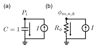
Figure 1: The SPICE equivalent circuit diagrams of (a) the TDGL equation, where $i=1,2,3$ and (b) the Poisson’s equation.

III.2 Poisson’s equation

To obtain the multi-domain potential profile and corresponding local electric field, we discretize Eq. (5) as

$$\begin{split}\nabla^{2}\phi=&\frac{\phi_{m+1,n,k}+\phi_{m-1,n,k}-2\phi_{m,n,k}}{dx^{2}}\\ &+\frac{\phi_{m,n+1,k}+\phi_{m,n-1,k}-2\phi_{m,n,k}}{dy^{2}}\\ &+\frac{\phi_{m,n,k+1}+\phi_{m,n,k-1}-2\phi_{m,n,k}}{dz^{2}}=g(\mathbf{P}),\end{split}$$ (10)

where $g(\mathbf{P})=\quantity(P_{1,1}+P_{2,2}+P_{3,3})/\quantity(\epsilon_{0}\kappa)$. By rearranging Eq. (10), one obtains

$$\begin{split}\frac{\phi_{m,n,k}}{R_{\phi}}&=-g(\mathbf{P})+\frac{\phi_{m+1,n,k}+\phi_{m-1,n,k}}{dx^{2}}\\ &\quad+\frac{\phi_{m,n+1,k}+\phi_{m,n-1,k}}{dy^{2}}+\frac{\phi_{m,n,k+1}+\phi_{m,n,k-1}}{dz^{2}}\\ &=I\quantity(\mathbf{P},\phi_{nn}),\end{split}$$ (11)

where $R_{\phi}=1/\quantity(2/dx^{2}+2/dy^{2}+2/dz^{2})$ and $\phi_{nn}$ represents the potentials of the nearest neighboring cells. Eq. (11) can be viewed as the voltage-current relationship of a constant resistor $R_{\phi}$ with the right hand side being a voltage-controlled current source.

If the finite screening lengths of the metal contacts are considered, the potential boundary conditions will depend on out-of-plane polarization as follows in order to account for the depolarization effect Chang et al. (2017b).

$$\begin{split}&V(z=0)=V_{\text{FE}}-\frac{\sigma_{s}\lambda_{1}}{\epsilon_{1}\epsilon_{0}}\\ &V(z=t_{\text{FE}})=0+\frac{\sigma_{s}\lambda_{2}}{\epsilon_{2}\epsilon_{0}},\end{split}$$ (12)

where $\sigma_{s}=\frac{P_{z}t_{\text{FE}}}{t_{\text{FE}}+\lambda_{1}/\epsilon_{1}+\lambda_{2}/\epsilon_{2}}$ is the screening charge density due to out-of-plane polarization, and $\lambda_{1,2}$ and $\epsilon_{1,2}$ are the screening lengths and relative dielectric constants of contacts {1,2}, respectively. The equivalent circuit diagrams of Eq. (1) and Eq. (5) are summarized in Fig. 1. Note that it is important to distinguish the total free charge density and polarization in an RFEC circuit Chang et al. (2018). In Fig. 2, the current flowing through the FE capacitor $I_{R}$ can be calculated as

$$I_{R}=\derivative{Q_{\text{FE}}}{t}=\derivative{t}\quantity(\epsilon_{0}\kappa\frac{V_{\text{FE}}}{t_{\text{FE}}}+P_{z})A,$$ (13)

where $Q_{\text{FE}}$ is the total free charge, $A$ is the capacitor cross-sectional area and $P_{z}$ is the average polarization in the out-of-plane direction. Note that it is more convenient to implement the contact module with Verilog-A based on Eq. (13). It is noteworthy that the measured charge is the total free charge $Q_{\text{FE}}$ instead of polarization charge according to Eq. (13).

IV Results and Discussion

Based on the phase field formalism, we solve the TDGL equation (Eq. (1)) and Poisson’s equation (Eq. (5)) for polarization charge and potential distributions to investigate the pulse switching dynamics of multi-domain HZO capacitors in an RFEC circuit. In this work, the baseline experimental measurements are extracted from Ref. Kobayashi et al. (2016), which demonstrated the transient responses of a TiN/Hf_0.7Zr_0.3O2/TiN capacitor under various pulse amplitudes. The parameters used in this work are summarized in Table 1.

Figure 2: The RFEC circuit diagram used in Ref. Kobayashi et al. (2016) and this work.

Table 1: Parameters Used For HZO in This Work

Parameter	Value
$\quantity(\lambda/\epsilon)_{1,2}$ (Å)	0.06, 0.06
$\kappa$	35
$t_{\text{FE}}$ $\mathrm{(}\mathrm{n}\mathrm{m}\mathrm{)}$	$10$ Kobayashi et al. (2016)
$\alpha_{1}$ (m/F)	$-4\text{\times}{10}^{8}$ Chang et al. (2018)
$\alpha_{11}$ $\mathrm{(}\mathrm{m}^{5}\mathrm{C}^{-2}\mathrm{/}\mathrm{F}\mathrm{)}$	$3.7\text{\times}{10}^{9}$ Chang et al. (2018)
$\alpha_{111}$ $\mathrm{(}\mathrm{m}^{9}\mathrm{C}^{-4}\mathrm{/}\mathrm{F}\mathrm{)}$	$1.1\text{\times}{10}^{9}$ Chang et al. (2018)
$G_{11}$ $\mathrm{(}\mathrm{m}^{3}\mathrm{/}\mathrm{F}\mathrm{)}$	dynamic
$L$ $\mathrm{(}\mathrm{\SIUnitSymbolOhm}\mathrm{m}\mathrm{)}^{-1}$	$2\text{\times}{10}^{-4}$ or dynamic
$R$ $\mathrm{(}\mathrm{\SIUnitSymbolOhm}\mathrm{)}$	20k Kobayashi et al. (2016)
Area $\mathrm{(}\mathrm{m}^{2}\mathrm{)}$	$7\text{\times}{10}^{-9}$ Kobayashi et al. (2016)

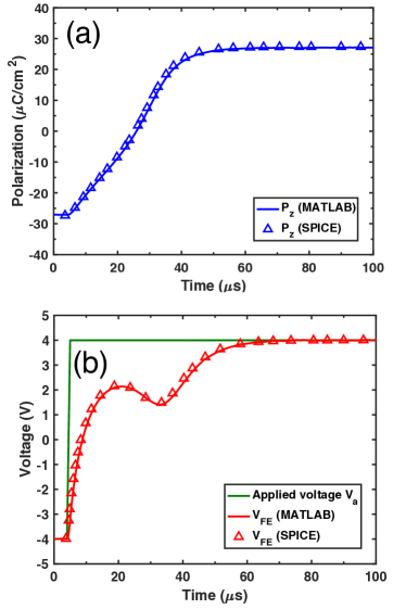
Figure 3: The comparisons between the semi-implicit Fourier-spectral method and SPICE circuit simulations of $P_{\text{z}}$ and $V_{\text{FE}}$ with $G_{11}=$1\text{\times}{10}^{-9}\text{\,}\mathrm{(}\mathrm{m}^{3}\mathrm{/}\mathrm{F}\mathrm{)}$$ at a pulse amplitude of $4\text{\,}\mathrm{V}$.

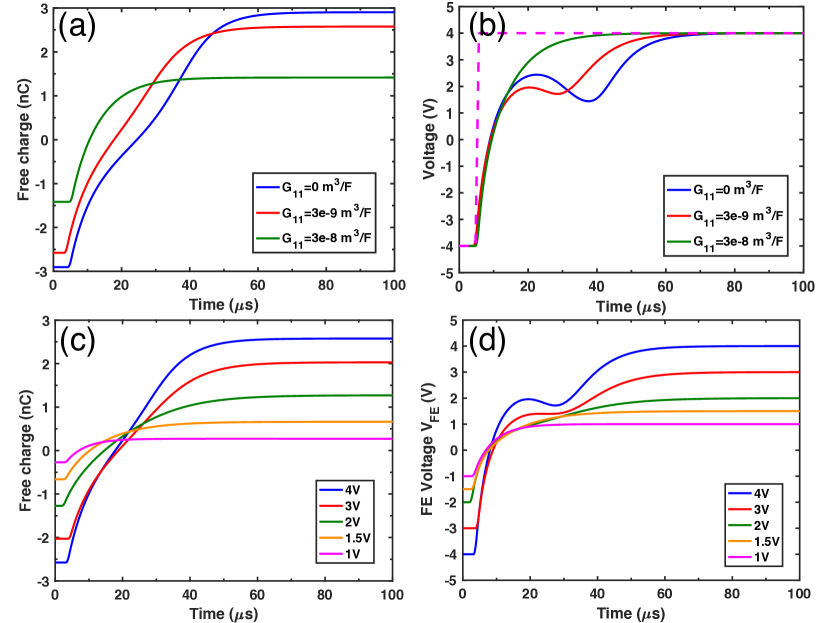
Figure 4: The SPICE simulations of (a) charge switching dynamics and (b) $V_{\text{FE}}$ transient responses with various $G_{11}$ values under a voltage pulse of $4\text{\,}\mathrm{V}$ (dashed line). (c) and (d) show transient responses of $Q_{\text{FE}}$ and $V_{\text{FE}}$ with $G_{11}$ correction under various pulse amplitudes.

IV.1 SPICE model initialization and validation

In our simulations, we first obtain the steady state multi-domain polarization distributions and potential profile under zero bias with polarization initialized with a zero-mean normal distribution. A negative voltage pulse is applied to the steady-state domain state to obtain the initial conditions for the pulse measurements.

To validate the proposed SPICE model, we also solve the TDGL equation (Eq. (1)) and Poisson’s equation (Eq. (5)) in MATLAB using the semi-implicit Fourier-spectral method Chen and Shen (1998). Fig. 3 shows the simulated transient responses from the SPICE simulator compared to those from the Fourier-spectral method with the same numerical settings and boundary conditions. For simplicity, the parasitic capacitance parallel to the FE capacitor is assumed to be small enough to be ignored in the RFEC circuit Hoffmann et al. (2016). The simulations presented below are all from the SPICE simulator if not mentioned elsewhere.

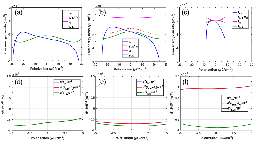
Figure 5: The top row shows transient energy profiles during pulse switching at various $G_{11}$. The corresponding free energy curvatures are in the bottom row. The $G_{11}$ values for {(a)(d)}, {(b)(e)} and {(c)(f)} are $0\text{\,}\mathrm{m}^{3}\mathrm{/}\mathrm{F}$, $3\text{\times}{10}^{-9}\text{\,}\mathrm{m}^{3}\mathrm{/}\mathrm{F}$ and $3\text{\times}{10}^{-8}\text{\,}\mathrm{m}^{3}\mathrm{/}\mathrm{F}$, respectively. The total free energy $f_{\text{tot}}=f_{\text{bulk}}+f_{\text{G}}+f_{\text{elec}}$.

IV.2 Effects of $G_{11}$ on the transient responses

From the experimental measurements in Ref. Kobayashi et al. (2016), the charge in the steady state is found to be suppressed at smaller pulse amplitudes. With our model, we find that the measured saturation free charges at various pulse amplitudes do not match those predicted by the phase field approach with a constant $G_{11}$. As a result, we propose that the gradient coefficient $G_{11}$ (and hence domain interaction) depends on the applied voltage. To verify this argument, we first examine how $G_{11}$ affects the transient behaviors at a pulse amplitude of $4\text{\,}\mathrm{V}$. In Fig. 4(a), the saturation charge decreases significantly as $G_{11}$ increases, which indicates that stronger domain interaction tends to suppress polarization switching. Moreover, the experimental measurements in Ref. Kobayashi et al. (2016) also show that the transient voltage drop disappears as the pulse voltage decreases. This finding is also captured by increasing $G_{11}$. As shown in Fig. 4(b), $V_{\text{FE}}$ dynamics acts like a normal dielectric capacitor and the voltage drop is no longer to be seen as domain interaction gets stronger (or larger $G_{11}$). Next, we extract the $G_{11}$ value for each pulse amplitude based on the saturation total free charge measured in Ref. Kobayashi et al. (2016). Fig. 6(a) shows the extracted $G_{11}$ at each pulse amplitude based on the experimentally measured FE free charge in the steady state. With extracted $G_{11}$, Fig. 4(c) and (d) show the transient responses of $Q_{\text{FE}}$ and $V_{\text{FE}}$ at various pulse amplitudes, which are qualitatively consistent with the experimental observations. Therefore, these simulation results imply that domain interaction of the HZO thin film is weaker under a larger voltage, which may be attributed to the breaking of spatial domain coupling under a large electric field.

IV.3 Effects of $G_{11}$ on the free energy profile

Now that we have shown that $G_{11}$ is dependent on the applied voltage, we investigate the effects of domain interaction on the observed transient responses in terms of the free energy profile. Fig. 5(a)–(c) show the transient energy profiles when polarization switches from the negative state to the positive state under a pulse of $4\text{\,}\mathrm{V}$ with increasing $G_{11}$. Without domain interaction ($G_{11}=$0\text{\,}\mathrm{m}^{3}\mathrm{/}\mathrm{F}$$), the bulk free energy exhibits a negative capacitance region (negative curvature) during polarization switching. With a nonzero $G_{11}$, the gradient free energy due to FE domain interaction shows a quadratic shape, and thus turns the negative curvature of the bulk free energy into a positive one as $G_{11}$ increases. Note that the extracted gradient free energy as a function of polarization is consistent with the parabolic shape obtained from the first-principles calculations Li et al. (2017). The corresponding free energy curvatures $\quantity(\partialderivative[2]{U}{P_{z}})$ near zero polarization are plotted in Fig. 5(d)–(f). The positive curvature of the total free energy with a larger $G_{11}$ explains how stronger domain interaction can suppress the transient NC. Since $G_{11}$ is voltage-dependent, the energy profile at various voltages will depend on how FE domains are interacted.

The voltage-dependence of the free energy curvature implies that FE capacitance can only be matched with a constant DE capacitance for charge-boost at a specific voltage based on the fact that the total free energy curvature is directly related to the FE capacitance Khan et al. (2014); Chang et al. (2018). Moreover, in Fig. 4(c) and (d), we use a constant value of $G_{11}$ to simulate the switching dynamics at an applied voltage pulse due to the short rise time of the pulse. In reality, $G_{11}$ varies when the applied voltage switches from low to high. This indicates that the frequency of the applied pulse affects the FE-DE capacitance matching as well.

Note that the electric free energy has a mathematical form as in Eq. (4) and hence does not affect the energy curvature, as can be seen in Fig. 5(d)–(f). As a result, our simulations also show that the gradient energy contribution $G_{11}\nabla^{2}P_{i}$ cannot be simply treated as an effective interaction field because the existence of gradient free energy changes the curvature of the total free energy landscape Saha et al. (2019).

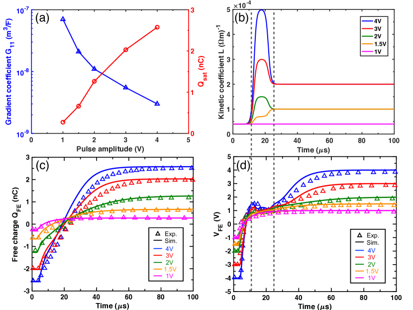
Figure 6: (a) The extracted $G_{11}$ values and the corresponding saturation free charge $Q_{\text{sat}}$ at various pulse amplitudes according to the experimental measurements in Ref. Kobayashi et al. (2016). (b) Kinetic coefficient dynamics during polarization switching at various pulse amplitudes. (c) The SPICE simulations of free charge switching dynamics at various pulse amplitudes compared with experiments in Ref. Kobayashi et al. (2016). (d) The SPICE simulations of $V_{\text{FE}}$ transient responses at various pulse amplitudes compared with experiments in Ref. Kobayashi et al. (2016).

IV.4 Dynamic kinetic coefficient

With extracted $G_{11}$ and a constant kinetic coefficient $L$, the measured saturation polarization can be well captured by the phase field framework. However, the voltage responses during the transient NC are not consistent with experiments. Therefore, we adopt a dynamic $L$ to further characterize the domain viscosity variations during polarization switching. Fig. 6(b) shows the transient kinetic coefficient $L$ at various pulse amplitudes. When $V_{\text{FE}}$ is below the coercive voltage $V_{c}$, the constant $L$ represents the inherent dielectric response. The larger $L$ in the time interval between the gray dashed lines demonstrates that the polarization switching speeds up due to the unstable nature of the NC region. As the FE capacitance goes back to a positive value, $L$ decreases and the transient $V_{\text{FE}}$ recovers to a normal dielectric response. For smaller pulse amplitudes, the energy curvature is positive during polarization switching due to stronger domain interaction, and therefore the transient responses of the FE are similar to DE responses without a voltage drop. Compared with measurements in Ref. Kobayashi et al. (2016), the simulation results of total free charge $Q_{\text{FE}}$ and FE voltage $V_{\text{FE}}$ with various pulse amplitudes are shown in Fig. 6(c) and (d).

Although our simulations show reasonable trends of the measured transient responses, there are still some discrepancies between the simulations and experiments, which may result from the elastic free energy. Because HZO thin films are not classical perovskites, the crystal structures and the related elastic contributions to the total free energy need further experimental investigations, which is beyond the scope of this paper. Further simulations that include broad distributions of bulk Landau parameters show insignificant impacts on the transient responses and confirm the dominant effects of the gradient coefficient sup . However, the gradient coefficient and kinetic coefficient may also have spatial distributions due to the multi-domain nature of HZO Hoffmann et al. (2016, 2018).

V Conclusion

In summary, the first physics-based circuit compatible SPICE model for multi-domain ferroelectric materials is developed and calibrated with experimental measurements. With this model, we investigate the effect of domain interaction on the transient responses of HZO capacitors under a voltage pulse in an RFEC circuit. We find that FE domain interaction depends on the applied voltage and plays an important role in the dynamic responses of polarization switching and the transient NC effect. By studying how domain interaction affects the total free energy curvature, we show that the effect of domain interaction cannot be viewed as an effective electric field. More importantly, the voltage-dependent domain interaction indicates that FE-DE capacitance matching can only be achieved at a specific voltage and frequency. Furthermore, the dynamic nature of FE domain viscosity at a voltage pulse is explored based on the experimental measurements. This work explores the physical roles that phenomenological parameters play in microscopic switching mechanisms for multi-domain HZO capacitors, and the proposed circuit model shows the potential for the analyses of HfO2-based ferroelectrics at device and circuit levels.

References

- Valasek (1920) J. Valasek, MSc thesis, Univ. Minnesota (1920).
- Salahuddin and Datta (2008) S. Salahuddin and S. Datta, Nano Letters 8, 405 (2008), doi: 10.1021/nl071804g, http://dx.doi.org/10.1021/nl071804g .
- Garcia and Bibes (2014) V. Garcia and M. Bibes, Nature Communications (2014).
- Hsu et al. (2018) C.-S. Hsu, C. Pan, and A. Naeemi, IEEE Electron Device Letters 39, 765 (2018).
- Moore (1998) G. Moore, Proceedings of the IEEE 86, 82 (1998).
- Khan et al. (2014) A. I. Khan, K. Chatterjee, B. Wang, S. Drapcho, L. You, C. Serrao, S. R. Bakaul, R. Ramesh, and S. Salahuddin, Nature Materials 14, 182 (2014).
- Gao et al. (2014) W. Gao, A. Khan, X. Marti, C. Nelson, C. Serrao, J. Ravichandran, R. Ramesh, and S. Salahuddin, Nano Letters 14, 5814 (2014).
- Appleby et al. (2014) D. J. R. Appleby, N. K. Ponon, K. S. K. Kwa, B. Zou, P. K. Petrov, T. Wang, N. M. Alford, and A. O’Neill, Nano Letters 14, 3864 (2014).
- Zubko et al. (2016) P. Zubko, J. C. Wojdeł, M. Hadjimichael, S. Fernandez-Pena, A. Sené, I. Luk’yanchuk, J.-M. Triscone, and J. Íñiguez, Nature 534, 524 (2016).
- Hoffmann et al. (2016) M. Hoffmann, M. Pešić, K. Chatterjee, A. I. Khan, S. Salahuddin, S. Slesazeck, U. Schroeder, and T. Mikolajick, Advanced Functional Materials 26, 8643 (2016).
- Chang et al. (2017a) S.-C. Chang, U. E. Avci, D. E. Nikonov, and I. A. Young, IEEE Journal on Exploratory Solid-State Computational Devices and Circuits 3, 56 (2017a).
- Böscke et al. (2011) T. S. Böscke, J. Müller, D. Bräuhaus, U. Schröder, and U. Böttger, Applied Physics Letters 99, 102903 (2011).
- Müller et al. (2012) J. Müller, T. S. Böscke, U. Schröder, S. Mueller, D. Bräuhaus, U. Böttger, L. Frey, and T. Mikolajick, Nano Letters 12, 4318 (2012).
- Sharma et al. (2017) P. Sharma, K. Tapily, A. K. Saha, J. Zhang, A. Shaughnessy, A. Aziz, G. L. Snider, S. Gupta, R. D. Clark, and S. Datta, in 2017 Symposium on VLSI Technology (IEEE, 2017).
- Kobayashi et al. (2016) M. Kobayashi, N. Ueyama, K. Jang, and T. Hiramoto, in 2016 IEEE International Electron Devices Meeting (IEDM) (IEEE, 2016).
- Chang et al. (2018) S.-C. Chang, U. E. Avci, D. E. Nikonov, S. Manipatruni, and I. A. Young, Physical Review Applied 9 (2018), 10.1103/physrevapplied.9.014010.
- Yuan et al. (2016) Z. C. Yuan, S. Rizwan, M. Wong, K. Holland, S. Anderson, T. B. Hook, D. Kienle, S. Gadelrab, P. S. Gudem, and M. Vaidyanathan, IEEE Transactions on Electron Devices 63, 4046 (2016).
- Hoffmann et al. (2018) M. Hoffmann, A. I. Khan, C. Serrao, Z. Lu, S. Salahuddin, M. Pešić, S. Slesazeck, U. Schroeder, and T. Mikolajick, Journal of Applied Physics 123, 184101 (2018).
- Saha et al. (2019) A. K. Saha, K. Ni, S. Dutta, S. Datta, and S. Gupta, Applied Physics Letters 114, 202903 (2019).
- Ishibashi and Takagi (1971) Y. Ishibashi and Y. Takagi, Journal of the Physical Society of Japan 31, 506 (1971).
- Kim et al. (2017) Y. J. Kim, H. W. Park, S. D. Hyun, H. J. Kim, K. D. Kim, Y. H. Lee, T. Moon, Y. B. Lee, M. H. Park, and C. S. Hwang, Nano Letters 17, 7796 (2017).
- Aziz et al. (2016) A. Aziz, S. Ghosh, S. Datta, and S. K. Gupta, IEEE Electron Device Letters 37, 805 (2016), doi: 10.1109/LED.2016.2558149.
- Asai et al. (2017) H. Asai, K. Fukuda, J. Hattori, H. Koike, N. Miyata, M. Takahashi, and S. Sakai, Japanese Journal of Applied Physics 56, 04CE07 (2017).
- Landau (1937) L. D. Landau, Zh. Eksp. Teor. Fiz 7, 19 (1937).
- Ginzburg (1945) V. L. Ginzburg, Zh. Eksp. Teor. Fiz 15, 739 (1945).
- Devonshire (1949) A. Devonshire, Phil. Mag 40, 1040 (1949).
- Hong et al. (2008) L. Hong, A. Soh, Y. Song, and L. Lim, Acta Materialia 56, 2966 (2008).
- Li et al. (2002) Y. L. Li, S. Y. Hu, Z. K. Liu, and L. Q. Chen, Applied Physics Letters 81, 427 (2002).
- Nambu and Sagala (1994) S. Nambu and D. A. Sagala, Physical Review B 50, 5838 (1994).
- Tagantsev (2008) A. K. Tagantsev, Ferroelectrics 375, 19 (2008).
- Agarwal et al. (2019) H. Agarwal, P. Kushwaha, Y.-K. Lin, M.-Y. Kao, Y.-H. Liao, A. Dasgupta, S. Salahuddin, and C. Hu, IEEE Electron Device Letters 40, 463 (2019).
- Wang and Zhang (2006) J. Wang and T.-Y. Zhang, Physical Review B 73 (2006), 10.1103/physrevb.73.144107.
- Dutta et al. (2014) S. Dutta, D. E. Nikonov, S. Manipatruni, I. A. Young, and A. Naeemi, IEEE Transactions on Magnetics 50, 1 (2014).
- Chang et al. (2017b) S.-C. Chang, A. Naeemi, D. E. Nikonov, and A. Gruverman, Physical Review Applied 7 (2017b), 10.1103/physrevapplied.7.024005.
- Chen and Shen (1998) L. Chen and J. Shen, Computer Physics Communications 108, 147 (1998).
- Li et al. (2017) G. Li, X. Huang, J. Hu, and W. Zhang, Physical Review B 95 (2017), 10.1103/physrevb.95.144111.
- (37) See Supplemental Material for detailed simulations with spatially distributed bulk Landau coefficients.