Void formation in operator growth, entanglement, and unitarity

Abstract

The structure of the Heisenberg evolution of operators plays a key role in explaining diverse processes in quantum many-body systems. In this paper, we discuss a new universal feature of operator evolution: an operator can develop a void during its evolution, where its nontrivial parts become separated by a region of identity operators. Such processes are present in both integrable and chaotic systems, and are required by unitarity. We show that void formation has important implications for unitarity of entanglement growth and generation of mutual information and multipartite entanglement. We study explicitly the probability distributions of void formation in a number of unitary circuit models, and conjecture that in a quantum chaotic system the distribution is given by the one we find in random unitary circuits, which we refer to as the random void distribution. We also show that random unitary circuits lead to the same pattern of entanglement growth for multiple intervals as in $(1+1)$-dimensional holographic CFTs after a global quench, which can be used to argue that the random void distribution leads to maximal entanglement growth.

I Introduction

The Heisenberg evolution of operators in a quantum many-body system is in general extremely complicated. But during the last decade, remarkable universalities have been found, such as ballistic growth of operators Roberts and growth of operator entanglement prosen1 ; prosen2 ; dubail ; JHN . Such universal properties have played an important role in diverse problems like scrambling of quantum information, quantum many-body chaos, and entanglement growth during thermalization (see e.g. Shenker1 ; abanin ).

In this paper, we discuss another universal feature of operator evolution: an operator can develop a void during its evolution. More explicitly, considering a spatial region $A$ within the “lightcone” of an initial operator ${{\mathcal{O}}}$, we can decompose its time evolution ${{\mathcal{O}}}(t)$ as

$${{\mathcal{O}}}(t)={{\mathcal{O}}}_{1}(t)+{{\mathcal{O}}}_{2}(t),\qquad{{\mathcal{O}}}_{1}(t)=\tilde{{\mathcal{O}}}_{\bar{A}}\otimes{\mathbf{1}}_{A}$$ (1)

where ${\mathbf{1}}_{A}$ denotes the identity operator in $A$, $\tilde{{\mathcal{O}}}_{\bar{A}}$ is some operator in $\bar{A}$ (the complement of $A$), and ${{\mathcal{O}}}_{2}(t)$ is an operator whose projection onto $A$ is orthogonal to ${\mathbf{1}}_{A}$. Here we assume that the system has a finite-dimensional Hilbert space and tensor product structure associated with spatial regions. See Fig. 1 for an illustration. Given the space of all operators is a Hilbert space, we can also associate a weight or “probability” for ${{\mathcal{O}}}(t)$ to develop a void in region $A$

$$P_{{{\mathcal{O}}}}^{(A)}(t)={\mathop{\rm Tr}\left({{\mathcal{O}}}_{1}^{\dagger}(t){{\mathcal{O}}}_{1}(t)\right)\over\mathop{\rm Tr}\left({{\mathcal{O}}}^{\dagger}(t){{\mathcal{O}}}(t)\right)}\ .$$ (2)

Below we will refer to the presence of ${{\mathcal{O}}}_{1}(t)$ in ${{\mathcal{O}}}(t)$ as void formation. Void formation is present in both integrable and chaotic systems, and is required by unitarity. We will show that it has important implications for unitarity of entanglement growth. For example, evolving from an initial product state, it is the contribution from ${{\mathcal{O}}}_{1}(t)$ that ensures $S_{A}(t)=S_{\bar{A}}(t)$, where $S_{A}$ is the entanglement entropy for region $A$. Further, we will show that void formation is responsible for generating mutual information and multipartite entanglement among disjoint regions during the evolution of a system, as we illustrate using a cartoon picture in Fig. 2. We will also derive a number of general constraints on probability distributions of void formation from unitarity, which are applicable to both chaotic and integrable systems.

Figure 1: An operator ${{\mathcal{O}}}$ in a many-body system can develop a “void” under time evolution, where nontrivial parts of ${{\mathcal{O}}}_{1}(t)$ (introduced in (1)) are separated by a region of identity operators. In the example shown above in one spatial dimension, the operator has nontrivial single-site operators at blue sites, and the identity at white sites.

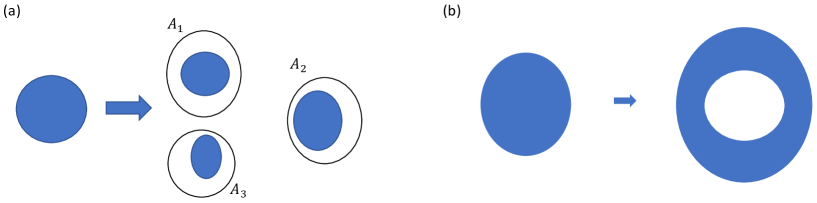
Figure 2: In more than one spatial dimension, void formation can either break up a single operator into disconnected parts, as in (a), or form a hole in an operator, as in (b). In the figure, shaded regions indicate where the operator has nontrivial support. A process like (a) contributes to multipartite entanglement between the three disjoint regions $A_{1}$, $A_{2}$, and $A_{3}$.

To develop intuition for probability distributions of void formation, we study three types of unitary circuit models in one spatial dimension: (i) the random unitary model of nahum1 ; frank ; nahum2 , which can be considered a minimal model for quantum chaotic systems; (ii) a “free propagating” model hong_mark in which entanglement can only be spread, but not created, which may thus be considered a proxy for free theories; (iii) a circuit built from perfect tensors qi , which may be considered a model for interacting integrable systems. In the free-propagating and perfect tensor models, patterns of void formation depend sensitively on the initial operator. In particular, in the perfect tensor circuit model, void formation exhibits a fractal structure.

In the random unitary circuit, we find at sufficiently late times

$$P^{(A)}_{{\mathcal{O}}}={1\over d_{A}^{2}}=e^{-2S_{\rm eq}^{(A)}}$$ (3)

where $d_{A}$ is the dimension of local Hilbert space in region $A$. After the second equality, we have written the expression in a form which is generalizable to continuum systems, with $S_{\rm eq}^{(A)}$ the equilibrium entropy of $A$. It is natural to conjecture that (3), to which we will refer as the random void distribution from now on, holds for generic operators in general chaotic systems at sufficiently late times. While (3) is very small for a macroscopic region $A$, for certain processes the number of contributing operators can be exponentially large, leading to significant physical effects.

As an illustration, we show that together with the assumption of sharp light-cone growth of operators, the random void distribution (3) fully determines the second Renyi entropy of an arbitrary number of disjoint intervals in random unitary circuits in the limit of large one-site Hilbert space dimension. Furthermore, surprisingly, the resulting expression coincides exactly with the von Neumann entropy after a global quench in $(1+1)$-dimensional holographic systems. On the one hand, this indicates that the random void distribution (3) may underlie operator evolution in holographic systems. On the other hand, in the light of the fact that the holographic expression maximizes the evolution of entanglement entropy in all $(1+1)$-dimensional systems hong_mark , we are led to conclude that together with sharp light-cone growth, the random void distribution maximizes entanglement growth.

The plan of this paper is as follows. In Sec. II, after describing in detail our general set-up, we discuss implications of void formation for unitarity of entanglement growth and generation of mutual information and multi-partite entanglement, as well as constraints on void formation from requiring unitarity. In Sec. III, we discuss the random circuit model, derive the random void distribution (3), and discuss its implications. In Sec. IV, we discuss void formation in the free propagation and perfect tensor models. We conclude in Sec. V with future directions. We have included a number of Appendices for technical details.

II Void formation and implications

In this section, we first describe our general setup, and then derive some simple constraints from unitarity on void formation during Heisenberg evolution.

II.1 Setup

For convenience, we will consider a one-dimensional lattice system with a finite-dimensional Hilbert space at each site. The discussion generalizes immediately to higher dimensions. We comment on generalizations to systems with an infinite local Hilbert space in the discussion section, Sec. V.

The Hilbert space at a site $i$ will be denoted as ${{\mathcal{H}}}_{i}$, and is taken to have dimension $q$. The full Hilbert space is ${{\mathcal{H}}}=\otimes{{\mathcal{H}}}_{i}$, and has dimension $q^{L}$, where $L\to\infty$ is the system size. Operators at a single site form a Hilbert space of dimension $q^{2}$, which will be denoted as ${{\mathcal{G}}}_{i}$. Operators of the full system form a Hilbert space ${{\mathcal{G}}}=\otimes_{i}{{\mathcal{G}}}_{i}$ of dimension $q^{2L}$. We will use $O_{a}^{i},a=0,1,\cdots q^{2}-1$, to denote an orthonormal basis of ${{\mathcal{G}}}_{i}$ which is normalized as

$$\mathop{\rm tr}((O_{a}^{i})^{\dagger}O_{b}^{i})=q{{\delta}}_{ab},\qquad O_{0}^{i}={\mathbf{1}}_{i}$$ (4)

where ${\mathbf{1}}_{i}$ is the identity operator of ${{\mathcal{H}}}_{i}$, and there is no summation over $i$ in the above equation. Orthogonality with $O_{0}^{i}$ implies $O_{a}^{i},a=1,\cdots q^{2}-1$, are all traceless. A convenient choice of basis which we will use throughout the paper is

$$O_{a}=X^{s_{1}}Z^{s_{2}},\qquad s_{1},s_{2}=0,1,\cdots q-1$$ (5)

where $X$ and $Z$ are respectively the shift and clock matrices. An orthonormal basis for ${{\mathcal{G}}}$, which will be denoted as ${{\mathcal{O}}}_{\alpha},{\alpha}=0,1,\cdots q^{2L}-1$, can be obtained from tensor products of $\{O_{a}^{i}\}$. These basis operators satisfy

$$\mathop{\rm Tr}{{\mathcal{O}}}_{\alpha}^{\dagger}{{\mathcal{O}}}_{\beta}={{\delta}}_{{\alpha}{\beta}}~{}q^{L}\ .$$ (6)

${{\mathcal{O}}}_{0}$ is the identity operator for the full Hilbert space ${{\mathcal{H}}}$, and all other ${{\mathcal{O}}}_{\alpha}$’s are traceless.

Under time evolution,

$${{\mathcal{O}}}_{\alpha}(t)=U^{\dagger}(t){{\mathcal{O}}}_{\alpha}U(t)=\sum_{\beta}c_{\alpha}^{\beta}(t){{\mathcal{O}}}_{\beta}$$ (7)

where $U(t)$ denotes the evolution operator. From unitarity of $U(t)$,

$$\sum_{\beta}|c_{\alpha}^{\beta}(t)|^{2}=1\ .$$ (8)

We can interpret $|c_{\alpha}^{\beta}(t)|^{2}$ as the probability of operator ${{\mathcal{O}}}_{\alpha}$ evolving to ${{\mathcal{O}}}_{\beta}$. Systems with a local Hamiltonian have an effective light-cone speed $v_{c}$ for how fast an operator can grow with time LR , so that $|c_{\alpha}^{\beta}(t)|^{2}\approx 0$ for ${{\mathcal{O}}}_{\beta}$ not contained within the light-cone of ${{\mathcal{O}}}_{\alpha}$.

For the purpose of not obscuring the conceptual picture with technicalities, throughout this paper, we will consider a particularly simple form of operator evolution in which the end points of an operator of interest move at the light-cone speed $v_{c}$ in opposite directions. We will refer to this assumption as sharp light-cone growth. See Fig. 3. From now on we will set $v_{c}=1$. Causality imposed by the light-cone structure will play a key role in the subsequent discussion. Throughout the paper, if not mentioned explicitly, we will always consider $q$ large and ignore subleading $1/q$ corrections. The qualitative picture does not change in more general situations, but the story becomes technically more complex, and will be treated elsewhere.

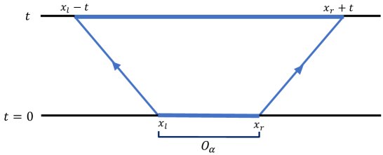
Figure 3: Under time-evolution, the end points of an operator ${{\mathcal{O}}}_{\alpha}$ move at the light-cone speed $v_{c}=1$ in opposite directions. The initial operator with endpoints at $x_{l}$ and $x_{r}$ can become a superposition of many final operators at time $t$, each of which have endpoints $x_{l}-t$ and $x_{r}+t$.

The statement about light-cone growth does not say anything about the internal structure of an operator under time evolution. A basic question addressed in this paper is: can the operator develop a void in some region between its endpoints, and if so, what are the implications of this process? We say an operator has a void in some region $A$ (which can have disconnected components) if it is a superposition of operators the form $\tilde{{\mathcal{O}}}\otimes{\mathbf{1}}_{A}$, where ${\mathbf{1}}_{A}$ denotes the identity operator in $A$ and $\tilde{{\mathcal{O}}}$ is some operator which has nontrivial support in all disconnected parts of $\bar{A}$ (the complement of $A$). Then the probability for a basis operator ${{\mathcal{O}}}_{\alpha}$ to develop a void in region $A$ at time $t$ is

$$P_{{{\mathcal{O}}}_{\alpha}}^{(A)}(t)=\sum_{{\beta}\;\text{with void in $A$}}|c_{\alpha}^{\beta}(t)|^{2}\ .$$ (9)

A main goal of this paper is to explore the role of void formation in the entanglement structure of a system. A good observable for this purpose is the evolution of the second Renyi entropy, which can be expressed in terms of operator growth  abanin ; MS ; nahum1 ; frank . Suppose at $t=0$, the system is described by a homogeneous pure product state, $\rho_{0}=\otimes_{i}\rho_{i}$, where $i$ runs over all sites of the system and $\rho_{i}$ is a pure state which is the same for all sites. It is convenient to choose a basis so that

$$\rho_{i}={1\over q}\left({\mathbf{1}}_{i}+Z_{i}+Z^{2}_{i}+\cdots+Z^{q-1}_{i}\right)$$ (10)

with $Z_{i}$ the clock matrix at site $i$, and thus

$$\rho_{0}={1\over q^{L}}\sum_{{\alpha}\in I}{{\mathcal{O}}}_{\alpha}$$ (11)

where $I$ denotes the set of operators which can be built from powers of $Z_{i}$’s. Note that the space $I$ is $q^{L}$-dimensional, in contrast to the $q^{2L}$-dimensional full space of operators.

Under time-evolution, the reduced density matrix for some region $A$ is given by

$$\rho_{A}(t)={\rm Tr}_{\bar{A}}\rho(t)={1\over q^{L}}\sum_{{\alpha}\in I}{\rm Tr}_{\bar{A}}{{\mathcal{O}}}_{\alpha}(t)={1\over q^{|A|}}\sum_{{\alpha}\in I}\sum_{{\beta}\in A}c_{{\alpha}}^{\beta}(t){{\mathcal{O}}}_{\beta}$$ (12)

where we have used (7), and the fact that due to tracelessness of all nontrivial basis operators, only operators of the form ${{\mathcal{O}}}_{\beta}\otimes{\mathbf{1}}_{\bar{A}}$ with ${{\mathcal{O}}}_{\beta}$ an operator in region $A$ (denoted by ${\beta}\in A$) contribute to ${\rm Tr}_{\bar{A}}{{\mathcal{O}}}_{\alpha}(t)$. $|A|$ denotes the size of region $A$. The second Renyi entropy for $A$ can then be written as

$$e^{-S_{2}^{(A)}(t)}={\rm Tr}_{A}\rho_{A}^{2}(t)={1\over q^{|A|}}\sum_{{\alpha}_{1},{\alpha}_{2}\in I}\sum_{{\beta}\in A}c_{{\alpha}_{1}}^{\beta}(t)c_{{\alpha}_{2}}^{{\beta}*}(t)\ .$$ (13)

We will now make a further simplification by ignoring the off-diagonal terms (i.e. terms with ${\alpha}_{1}\neq{\alpha}_{2}$) in (13). For chaotic systems, one expects the phases of $c_{\alpha}^{\beta}$ to be random, so that the off-diagonal terms are suppressed by order $O(q^{-|A|})$ compared with diagonal terms MS . For integrable systems one cannot make this argument. Nevertheless, there are often situations where the off-diagonal terms vanish identically. This is the case for all the explicit examples we discuss in Sec. III and Sec. IV. We then find

$$e^{-S_{2}^{(A)}(t)}={1\over q^{|A|}}N_{A}(t),\quad N_{A}(t)\equiv\sum_{{\alpha}\in I}\sum_{{\beta}\in A}|c_{{\alpha}}^{\beta}(t)|^{2},\quad S_{2}^{(A)}=|A|\log q-\log N_{A}(t)\ .$$ (14)

$N_{A}(t)$ has a simple physical interpretation: it is the expected number of operators in the set $I$ contained within region $A$ at time $t$. Note that $N_{A}\geq 1$, as $O_{\alpha}=\mathbf{1}$ always contributes $1$ to the above sum. For our later discussion, it is convenient to introduce a function $N(A,B;t)$, defined as the expected number of initial operators in $I$ from some region $B$ that are contained in $A$ at time $t$, i.e.

$$N(A,B;t)\equiv\sum_{{\alpha}\in I\cap B}\sum_{{\beta}\in A}|c_{\alpha}^{\beta}(t)|^{2},$$ (15)

and a void formation function $G(A,B;t)$, defined as the expected number of initial operators in $I$ from some region $B$ that develop a void in $A$ at time $t$, i.e.,

$$G(A,B;t)\equiv\sum_{{\alpha}\in I\cap B}\sum_{{\beta}\;\text{with void in $A$}}|c_{\alpha}^{\beta}(t)|^{2}=\sum_{{\alpha}\in I\cap B}P_{{{\mathcal{O}}}_{\alpha}}^{(A)}(t)\ .$$ (16)

$G(A,B;t)$ is closely related to $N(\bar{A},B;t)$, but in $G(A,B;t)$ the final operators must be supported on all disconnected parts of $\bar{A}$. Again by definition, $N(A,B;t),G(A,B;t)\geq 1$, as we always have a contribution of 1 from the identity operator.

Throughout the paper, we will denote the union of two regions $A_{1}\cup A_{2}$ simply as $A_{1}A_{2}$.

II.2 Upper bound on average probability for void formation

To give some intuition for the motivation behind (3), we first discuss the average probability for an operator to become trivial in a given region.

Consider a Hilbert space ${{\mathcal{G}}}$ of dimension $d$ and a subspace ${{\mathcal{G}}}^{\prime}\subset{{\mathcal{G}}}$ of dimension $d^{\prime}$, with $P$ the projector onto ${{\mathcal{G}}}^{\prime}$. For a vector $\ket{\psi}\in{{\mathcal{G}}}$, the probability that it transitions into a state in ${{\mathcal{G}}}^{\prime}$ under a unitary transformation is given by

$$p=\mathop{\rm Tr}\left(PU\ket{\psi}\bra{\psi}U^{\dagger}\right)\ .$$ (17)

The average probability $\bar{p}$, obtained by averaging $\ket{\psi}$ over all unit vectors in ${{\mathcal{G}}}$ with the unitarily invariant Haar measure, is then

$$\bar{p}={1\over d}\mathop{\rm Tr}P={d^{\prime}\over d}\ .$$ (18)

We take ${{\mathcal{G}}}$ to be the Hilbert space of all operators with dimension $d=q^{2L}$, and ${{\mathcal{G}}}^{\prime}$ to be the set of operators which are the identity in region $A$, which is a subspace of dimension $d^{\prime}=q^{2(L-|A|)}$. We thus conclude that the average probability for an operator to be trivial in region $A$ is

$$\bar{p}=q^{-2|A|}={1\over d_{A}^{2}}\ .$$ (19)

Apart from the assumption that $U$ is unitary, (19) is independent of $U$ and does not depend on the region $A$ other than through its size. Note that (19) gives the probability for an operator to be trivial in $A$, which is larger than the probability for developing a void in $A$, as it also includes final operators which are trivial in some disconnected parts of $\bar{A}$.

Note that if we do not average $\ket{\psi}$ but instead take $U$ to be a random unitary matrix with the Haar distribution, we find the same answer. This is the motivation for the name “random void distribution”  for (3).

II.3 Unitarity of entanglement growth for one interval

We now present a simple argument which shows that void formation plays a crucial role in ensuring that the entanglement growth of a system after a global quench is compatible with unitarity. The argument can be used to derive a constraint on void formation by requiring unitarity.

To find the second Renyi entropy (14) for some finite interval $A$, we need to find the expected number of operators in $I$ which fall into $A$ as a function of time. The sharp light-cone growth of operators depicted in Fig. 3 makes the counting very simple abanin ; MS . Let us denote the intersection of the past domain of dependence of region $A$ with the $t=0$ slice as $D(A)$. It then follows from the light-cone structure that all operators in $D(A)$ are contained within region $A$ at time $t$, while an operator with a nontrivial part outside $D(A)$ at $t=0$ will evolve into operators with nontrivial parts outside $A$. See Fig. 4. Thus only the initial operators in $D(A)$ contribute to $N_{A}(t)$, and each of them contributes a probability $1$. $N_{A}(t)$ is then given by the number of basis operators in the set $I\cap D(A)$, which leads to

$$N_{A}(t)=\begin{cases}q^{|D(A)|}=q^{|A|-2t}&t<{|A|\over 2}\cr 1&t>{|A|\over 2}\end{cases}\quad{\Longrightarrow}\quad S^{(A)}_{2}(t)=\begin{cases}2{s_{\rm eq}}t&t<{|A|\over 2}\cr{s_{\rm eq}}|A|&t>{|A|\over 2}\end{cases},\quad{s_{\rm eq}}\equiv\log q\ .$$ (20)

Physically, under evolution, initial basis operators localized in $A$ move out at the lightcone speed in both directions. When an operator develops a nontrivial part outside $A$, it ceases to contribute to $N_{A}(t)$ and increases the entropy of $A$. At time $t$, the only operators remaining inside $A$ are those which are initially localized in $D(A)$. When $t>{|A|\over 2}$, $D(A)$ is empty, with all nontrivial operators having evolved outside $A$. The only contribution to $N_{A}(t)$ is from the identity, and the entropy saturates. One can in fact show that with the sharp light-cone growth, all the Renyi and von Neumann entropies for a single interval $A$ are also given by (20), and $\rho_{A}$ is unitarily equivalent to a reduced density matrix in which the region $A-D(A)$ is maximally entangled with $\bar{A}$ while $D(A)$ remains pure, as in the picture of the “entanglement tsunami” Liu:2013iza .

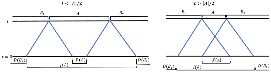
Figure 4: Left: $t<|A|/2$. Right: $t>|A|/2$. $D(A)$ is the intersection of the past domain dependence of $A$ with the $t=0$ slice, which becomes empty for $t>|A|/2$. $J(A)$ is the region at $t=0$ which is causally connected with $A$. At $t<|A|/2$, every operator in $J(A)$ has zero probability of transitioning to a final operator contained in $\bar{A}=B_{1}B_{2}$. At $t\geq|A|/2$, an operator in $J(A)$ can transition to an operator contained in $\bar{A}$ if it develops a void in $A$.

This discussion provides a simple explanation for the linear growth of entanglement entropy and its saturation, and shows that such behavior has its physical origin in ballistic operator growth, regardless of whether the system is chaotic or integrable. But at this stage, there is an apparent violation of unitarity. Applying the above discussion to $S^{(\bar{A})}_{2}(t)$, we obtain the same behavior as (20) with $|A|$ replaced by $|\bar{A}|=L-|A|\to\infty$, which is inconsistent with $S^{(A)}_{2}(t)=S^{(\bar{A})}_{2}(t)$ for $t\geq|A|/2$. That is, instead of growing indefinitely, under unitary evolution $S^{(\bar{A})}_{2}(t)$ must also saturate at ${s_{\rm eq}}|A|$ for $t>|A|/2$.

The way out is as follows. Let us denote the region at $t=0$ which is in causal contact with $A$ as $J(A)$ (see Fig. 4), and consider an initial operator of the form ${{\mathcal{O}}}_{J(A)}\otimes{{\mathcal{O}}}_{D(\bar{A})}$ with ${{\mathcal{O}}}_{J(A)}$ a nontrivial operator in $J(A)$. In the discussion above, such an operator was assumed to have no contribution to $N_{\bar{A}}(t)$, as naively its time evolution will be nontrivial in $A$. But this is incorrect; such operators can contribute to $N_{\bar{A}}(t)$ if ${{\mathcal{O}}}_{J(A)}$ develops a void in $A$. Moreover, due to causality, the behavior of ${{\mathcal{O}}}_{J(A)}$ in region $A$ under time evolution–including the probability of developing a void–should be independent of ${{\mathcal{O}}}_{D(\bar{A})}$. This means that $N_{\bar{A}}(t)$ can be written in a factorized form

$$N_{\bar{A}}(t)=q^{|\bar{A}|-2t}N(\bar{A},J(A);t),$$ (21)

where the factor $q^{|\bar{A}|-2t}$ is the number of basis operators in $I\cap D(\bar{A})$, and the function $N$ was introduced in (15). When $A$ is a single interval, it is clear from causality that

$$N(\bar{A},J(A);t)=G(A,J(A);t)$$ (22)

where as defined in (16), $G(A,J(A);t)$ is defined as the expected number of initial basis operators in $J(A)$ that develop a void in $A$. For $S_{2}^{(A)}=S_{2}^{(\bar{A})}$, we need

$$G(A,J(A);t)=\begin{cases}1&t<{|A|\over 2}\cr q^{2t-|A|}&t>{|A|\over 2}\end{cases}\ .$$ (23)

The second line of (23) has the simple interpretation that the average probability of the $q^{|J(A)|}=q^{|A|+2t}$ basis operators in $J(A)\cap I$ to develop a void in $A$ is $q^{-2|A|}$. Also note that $q^{2t-|A|}=q^{|X|}$, where the region $X$ is as shown in Fig. 4. For an operator to develop a void in $A$, from causality it must be supported in region $X$. Note that while there are some similarities, equation (23) is different in nature from (19). Equation (19) is a purely kinematic statement, while (23) contains the dynamical input of the sharp light-cone growth and refers to an average over a more restricted set of initial operators.

Now consider the following “Renyi mutual information” between regions $B_{1}$ and $B_{2}$ in Fig. 4:

$$I_{2}(B_{1},B_{2})\equiv S_{2}^{(B_{1})}+S_{2}^{(B_{1})}-S_{2}^{(\bar{A})},\quad\bar{A}=B_{1}B_{2}\ .$$ (24)

From (21) and (22), we find that this quantity is fully controlled by the expected number of operators developing a void

$$I_{2}(B_{1},B_{2})=\log G(A,J(A);t)=\begin{cases}0&t<{|A|\over 2}\cr{s_{\rm eq}}(2t-|A|)&t>{|A|\over 2}\end{cases}\ .$$ (25)

This result is intuitively appealing: when an operator develops a void in an interval $A$, it leads to mutual information between regions separated by $A$.

We stress that (23), and accordingly (25), are constrained by unitarity and should apply to any system, integrable or chaotic, which has sharp light-cone growth for the initial set of operators. We will see that (23) is indeed satisfied in various exactly solvable unitary circuit models in Sec. III and Sec. IV.

II.4 Mutual information and multi-partite entanglement

Here we explore further implications of void formation, as well as general constraints on this process, by examining the Renyi entropy for two and more disjoint intervals. Extending (25), we first show that the mutual information between two disjoint finite intervals is determined by the void formation function $G(B,\tilde{B};t)$ for some appropriate regions $B$ and $\tilde{B}$. In a certain region of the parameter space, the corresponding mutual information is universal, determined by (23) from unitarity. We also derive new constraints on void formation from unitarity of entanglement growth for two intervals. For more disjoint intervals, we see that void formation in operator growth leads to multi-partite entanglement, and void formation functions provide new measures for characterizing multi-partite entanglement.

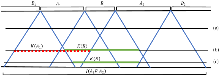
Figure 5: Different situations for two intervals. Different horizontal lines correspond to $t=0$ slices for (a) $t<|R|/2$; (b) $t>|l_{1}|/2$; (c) $t>|l_{2}|/2$. Here we take $|R|<|A_{1}|$ and thus $l_{1}=|A_{1}|$ and $l_{2}=|A_{2}|$.

Consider $S_{2}$ for a region $A=A_{1}A_{2}$ separated by an interval $R$. Without loss of generality, we can take $|A_{1}|\leq|A_{2}|$. For $t<|R|/2$, from causality, $N_{A}(t)$ of (14) factorizes into a product of the functions for $A_{1}$ and $A_{2}$

$$N_{A}(t)=N_{A_{1}}(t)N_{A_{2}}(t),\quad S_{2}^{(A)}(t)=S_{2}^{(A_{1})}(t)+S_{2}^{(A_{2})}(t),\quad t<{|R|\over 2}$$ (26)

where $N_{A_{1}}(t)$ denotes the contribution from initial operators in the region $D(A_{1})$ and is given by (20). For $t>{|R|\over 2}$, initial operators in the region $K(R)=J(R)\cap D(A_{1}RA_{2})$ (see Fig. 5) can now potentially form a void in region $R$ and thus contribute to $N_{A}(t)$

$$N_{A}(t)=N_{A_{1}}(t)N_{A_{2}}(t)G(R,K(R);t),$$ (27)

which gives

$$I_{2}(A_{1},A_{2};t)=\log G(R,K(R);t)\ .$$ (28)

For further discussion, it is convenient to introduce the following notation:

$$l_{1}\equiv{\rm max}(|A_{1}|,|R|),\quad l_{2}\equiv{\rm max}(|A_{2}|,|R|),\quad K(A_{1})\equiv J(A_{1})\cap D(B_{1}A_{1}R)\ .$$ (29)

Note that when $t<|R|/2$, we have the factorized form (26) in any theory with sharp light-cone growth. For $|A_{1}|/2>t>|R|/2$ (which can happen for $|A_{1}|>|R|$), we have $K(R)=J(R)$, and from (23)

$$I_{2}(A_{1},A_{2})={s_{\rm eq}}(2t-|R|)\ .$$ (30)

For $t>{|A|+|R|\over 2}$, $K(R)$ becomes an empty set, and thus $G(R,K(R);t)=1$. So for $t<l_{1}/2$ and for $t>{|A|+|R|\over 2}$, $G(R,K(R);t)$ and $I_{2}(A_{1},A_{2})$ have a universal form in all systems with sharp light-cone growth. For ${|A|+|R|\over 2}>t>l_{1}/2$, $K(R)\subset J(R)$, the behavior of $G(R,K(R);t)$ becomes system-dependent, and so does $I_{2}(A_{1},A_{2})$. Now consider the entropy for the region $\bar{A}=B_{1}RB_{2}$, for which

$$N_{\bar{A}}(t)=N_{B_{1}}(t)N_{B_{2}}(t)N(\bar{A},J(A_{1}RA_{2});t)\ .$$ (31)

Similar to the discussion immediately above, for $t\leq l_{1}/2$, the constraint (23) is enough to ensure $S_{2}^{(A)}=S_{2}^{(\bar{A})}$, but for $t>l_{1}/2$ new constraints arise. We find (see also Fig. 5)

$${l_{1}\over 2}<t\leq{l_{2}\over 2}:\quad G(R,K(R);t)=q^{|A_{1}|-|R|}G(A_{1},K(A_{1});t)$$ (32)

$$t>{l_{2}\over 2}:\quad G(R,K(R);t)=q^{|A|-|R|-2t}N(\bar{A},J(A_{1}RA_{2});t),$$ (33)

For $t>{|A|+|R|\over 2}$, with $G(R,K(R);t)=1$, we must have

$$N(\bar{A},J(A_{1}RA_{2});t)=q^{2t+|R|-|A|},\quad t>{|A|+|R|\over 2}\ .$$ (34)

If we take $A_{2}$ to be the entire semi-infinite region to the right of $R$, then both regions $K(A_{1})$ and $K(R)$ appearing in (32) and (33) depend only on $A_{1}$ and $R$, and $l_{2}/2\rightarrow\infty$, so (32) holds for all $t>l_{1}/2$. We can thus deduce from (32) a general constraint on the void formation functions for any two adjacent finite intervals $A$ and $B$ in an infinite system,

$$q^{|A|}G(A,K_{l}(A,B);t)=q^{|B|}G(B,K_{r}(A,B);t),~{}~{}~{}~{}t>\text{max}(|A|/2,|B|/2)$$ (35)

where

$$K_{l}(A,B)=J(A)\cap D(L_{1}AB),~{}~{}~{}~{}K_{r}(A,B)=J(B)\cap D(ABL_{2})$$ (36)

where $L_{1},L_{2}$ are the semi-infinite regions to the left of $A$ and to the right of $B$ respectively. The different regions appearing in (35) are shown in Fig. 6.

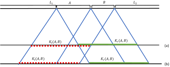
Figure 6: Regions $K_{l}(A,B)$ and $K_{r}(A,B)$ of (35) at a time $t<(|A|+|B|)/2$ in (a), and $t>(|A|+|B|)/2$ in (b). The condition (35) holds at all times $t>\text{max}(|A|/2,|B|/2)$.

The above discussion can be generalized to express the second Renyi entropy for any number of intervals in terms of appropriate void formation functions. On the one hand, by requiring $S_{2}^{(A)}(t)=S_{2}^{(\bar{A})}(t)$ for $A$ consisting of an arbitrary number of intervals, one can obtain further constraints on the void formation functions. On the other hand, with the full knowledge of the void formation functions, one should be able to deduce the expression for $S_{2}^{(A)}$ for any $A$. We will see an explicit example of this in Sec. III.3.

Now consider a region consisting of $n$ disjoint intervals $A=A_{1}\cdots A_{n}$ separated by intervals $R_{1},\cdots R_{n-1}$, as in Fig. 7. Then the void formation function $G(A,Q;t)$ gives a contribution to the entropy of the region $\bar{A}=R_{0}R_{1}\cdots R_{n}$, but does not contribute to the entropy of any region consisting of a proper subset of $\{R_{0},\cdots,R_{n}\}$. Thus void formation in $A$ leads to multi-partite entanglement among all disconnected regions in $\overline{A}$, which can be captured by the quantity $G(A,Q;t)$.

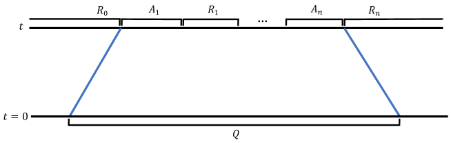
Figure 7: When initial operators in $Q$ develop a void in $A=A_{1}\cdots A_{n}$, this leads to multiple-partite entanglement among regions $R_{0},R_{1},\cdots R_{n}$. Here $Q$ is $J(A_{1}R_{1}\cdots R_{n-1}A_{n})$.

III Random void distribution and entanglement growth

In this section, we consider the probability distribution of void formation for a generic operator in the random unitary circuit model in the large $q$ limit. We show that it is given by the random void distribution (3). We then show that by assuming the random void distribution for all initial operators, we can correctly obtain the full expression for $S_{2}^{(A)}$ in the random circuit model for $A$ consisting of an arbitrary number of disjoint intervals. Surprisingly, the resulting expression is found to coincide with the von Neumann entropy for holographic systems. In the next section, we will contrast the random void distribution with the void formation properties of two Clifford circuit models (which may be seen as non-chaotic systems).

III.1 Random unitary circuits

We first describe briefly the setup of the random unitary circuit discussed in nahum1 ; frank ; nahum2 , and its main properties. Consider a time-evolution of the system as in Fig. 8, where the evolution operator $U(t)$ can be written as

$$U(t)=U_{t}U_{t-1}\cdots U_{0},$$ (37)

$$U_{0}=\cdots\otimes U_{0}^{0,1}\otimes U_{0}^{2,3}\otimes\cdots,\quad U_{1}=\cdots\otimes U_{1}^{-1,0}\otimes U_{1}^{1,2}\otimes\cdots\ .$$ (38)

Here we take discrete time steps, with $U_{n}$ corresponding to the evolution operator at the $n$-th step. $U^{i,i+1}_{n}$ is a $q^{2}\times q^{2}$ unitary matrix that acts on two neighboring sites $i$ and $i+1$ at $n$-th step, and each such matrix is averaged over the Haar measure independently. We will consider the limit of large $q$.

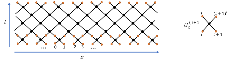
Figure 8: Unitary circuit for the time-evolution operator $U(t)$ (37)–(38) for $t=5$. The black circles represent unitary matrices $U^{i,i+1}_{t}$ acting on two adjacent sites $i$ and $i+1$. In the random circuit model, $U^{i,i+1}_{t}$ for each $i$ and $t$ is independently drawn from the Haar ensemble of $q^{2}\times q^{2}$ unitary matrices. Here in the first step of the time-evolution, we couple sites 0 and 1, 2 and 3, and so on, and in the second step we couple -1 and 0, 1 and 2, and so on. We explicitly show lattice sites of the system at $t=0$ and $t=1$ with the orange circles.

The random unitary circuit can be seen as a discretized model for chaotic quantum systems. It is manifestly unitary and local, but replaces the local interactions between neighboring spins in a realistic Hamiltonian system by random ones. It provides a powerful playground for studying chaotic systems, as many observables such as entanglement entropy, OTOCs, and operator spreading coefficients are analytically calculable, and the resulting behavior has been found to be consistent with numerical results of realistic chaotic spin-chain systems nahum1 ; frank ; swingle ; swingle2 ; levi .

Here are some features of the random circuit model in the large $q$ limit which are relevant for our discussion nahum1 ; frank ; nahum2 :

1. For a basis operator ${{\mathcal{O}}}_{\alpha}$ (introduced above (6)) with right and left endpoints given by $x_{r}$ and $x_{l}$ respectively, one finds

   $$\begin{gathered}\sum_{\begin{subarray}{c}{\beta}\text{ with left endpoint}\\ x_{l}-t,\text{ right endpoint }x_{r}+t\end{subarray}}\overline{\left|c_{{\alpha}}^{\beta}(t)\right|^{2}}=1+O(1/q)\end{gathered}$$ (39)

   which implies that the end points of any operator ${{\mathcal{O}}}$ move under time evolution in opposite directions with light cone speed $1$ as in Fig. 3. Here and below, an overline denotes an average over the random unitaries.

2. The calculation of the second Renyi entropy $S_{2}^{(A)}$ for a region $A$ can be reduced to computing the partition function of a classical Ising model on a triangular lattice. For $A$ consisting of a single interval, it has the form (20), consistent with the general argument presented earlier.

3. In the large $q$ limit,

   $$e^{-\overline{S_{2}^{(A)}}}=\overline{e^{-S_{2}^{(A)}}}={1\over q^{|A|}}\overline{N_{A}(t)}$$ (40)

   where $N_{A}(t)$ was defined in (14). Here the off-diagonal terms in (13) automatically vanish due to random averages. Furthermore, one has

   $$\overline{S_{2}^{(A)}}=\overline{S_{n}^{(A)}}=\overline{S^{(A)}},\quad\forall n>2,\quad n\in{\mathbb{{N}}}$$ (41)

   where $S^{(A)}$ denotes the von Neumann entropy. So our discussion below about $S_{2}$ can also be understood as being relevant for the von Neumann entropy.

III.2 Random void distribution

We now look at the probability distribution for a generic operator ${{\mathcal{O}}}$ to develop a void in some designated region $A$ in the random circuit model at large $q$.

We can expand ${{\mathcal{O}}}$ in terms of basis operators as

$${{\mathcal{O}}}=\sum_{\alpha}a_{\alpha}{{\mathcal{O}}}_{\alpha},\qquad{{\mathcal{O}}}(t)=\sum_{\alpha}\sum_{\beta}a_{\alpha}c_{\alpha}^{\beta}(t){{\mathcal{O}}}_{\beta},\quad\sum_{\alpha}|a_{\alpha}|^{2}=1.$$ (42)

Then under time evolution, the probability for ${{\mathcal{O}}}$ to have a void in $A$ is

$$\overline{P_{{\mathcal{O}}}^{(A)}(t)}=\sum_{{\beta}\,\text{with void in $A$}}\sum_{{\alpha}_{1},{\alpha}_{2}}a_{{\alpha}_{1}}a_{{\alpha}_{2}}^{*}\overline{c_{{\alpha}_{1}}^{{\beta}}(t)c_{{\alpha}_{2}}^{*{\beta}}(t)}=\sum_{\alpha}|a_{\alpha}|^{2}\overline{P_{{{\mathcal{O}}}_{\alpha}}^{(A)}(t)}$$ (43)

where $P_{{{\mathcal{O}}}_{\alpha}}^{(A)}$ was introduced in (9), and in the second equality the off-diagonal terms drop out due to the random average. In (43) by “${\beta}$ with void in $A$” we mean ${{\mathcal{O}}}_{\beta}$ should be trivial in $A$ and have support in each disconnected part of $\bar{A}$. For instance, in the case of $A=A_{1}A_{2}\cdots A_{n}$ in Fig. 7, ${{\mathcal{O}}}_{\beta}$ should be the identity in $A$ while being nontrivial in each of $R_{i}$’s. From now on, for notational simplicity we will suppress the explicit overline for averages.

$P_{{{\mathcal{O}}}_{\alpha}}^{(A)}(t)$ can be expressed as the partition function of a classical Ising model on a triangular lattice with boundary conditions specified by ${{\mathcal{O}}}_{\alpha}$ and $A$. We present the details of the calculation in Appendix A.2. For any operator ${{\mathcal{O}}}_{\alpha}$ which does not have an initial void, the final result is the random void distribution (RVD) already mentioned in the Introduction section

$$P_{{{\mathcal{O}}}_{\alpha}}^{(A)}(t)=\begin{cases}e^{-2{s_{\rm eq}}|A|}={1\over d_{A}^{2}}&t\geq{\rm max}\left({|A_{i}|\over 2},\forall i\right),A\in J^{+}({{\mathcal{O}}}_{\alpha})\cr 0&\text{otherwise}\end{cases}$$ (44)

where we have taken $A=A_{1}A_{2}\cdots A_{n}$ with $|A|=|A_{1}|+\cdots+|A_{n}|$, $J^{+}({{\mathcal{O}}}_{\alpha})$ denotes the region at time $t$ which is causally connected to ${{\mathcal{O}}}_{\alpha}$, and ${s_{\rm eq}}=\log q$. See Fig. 9. That to have a nonzero result we must have $A\in J^{+}({{\mathcal{O}}}_{\alpha})$ follows simply from causality. If any of the $A_{i}$ are not in $J^{+}({{\mathcal{O}}}_{\alpha})$, clearly ${{\mathcal{O}}}_{\alpha}$ cannot evolve into an operator which is nontrivial in all disconnected parts of $\bar{A}$.

Operators with initial voids can in general evolve to final operators that have support in all disconnected parts of $\bar{A}$ by two distinct kinds of processes. We can have processes where at some intermediate stage, the operator evolves to an operator without a void (if the initial voids are denoted by $G_{1},...,G_{m}$, such processes are allowed by causality only at $t>|G_{i}|/2$ for all $i$), which then splits to form a void in $A$. Another kind of process is one where different disconnected parts of the initial operator evolve to different disconnected parts of $\overline{A}$ without interacting with one another. Depending on the sizes and locations of the $G_{i}$, either of these types of processes can give the dominant contribution to $P_{{{\mathcal{O}}}_{\alpha}}^{(A)}(t)$ in the large $q$ limit. When the leading contribution is given by the former process, which can physically be seen as one of genuine “void formation,” we still have (44). When one of the latter types of processes is dominant, $P_{{{\mathcal{O}}}_{\alpha}}^{(A)}(t)$ is enhanced compared to (44). Nevertheless, for a generic operator (42), the part of the operator corresponding to ${{\mathcal{O}}}_{\alpha}$ with an initial void is suppressed due to a much smaller phase space. One can show that the enhancement from disconnected processes never overcomes the suppression. See Appendix A.2. Given that (44) is independent of ${{\mathcal{O}}}_{\alpha}$ other than through the causality constraint $A\in J^{+}({{\mathcal{O}}}_{\alpha})$, a generic operator ${{\mathcal{O}}}$ also satisfies (44).

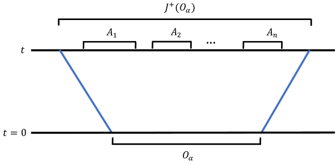
Figure 9: Regions $J^{+}({{\mathcal{O}}}_{\alpha})$ and $A_{1},A_{2},...,A_{n}$. In the random void distribution, the probability of forming a void in $A\equiv A_{1}A_{2}...A_{n}$ depends only on the lengths $|A_{1}|,...,|A_{n}|$.

Note that if we assumed that for a given initial operator, the probability of having any of the $q^{2}$ basis operators at any site between the endpoints of the operator at time $t$ is the same, then the probability $q^{-2|A|}$ would immediately follow: having a void in $A$ corresponds to fixing the operators at $|A|$ sites in the final operator to be one of $q^{2}$ options, while allowing the remaining operators to take any value. A similar ergodicity assumption was used in the operator growth model introduced in abanin . Equation (44) also applies to the random circuit model at a finite $q$ in the regime that region $A$ and $t$ are large (so that $q^{|A|},q^{t}$ are large), as we will discuss elsewhere.

From (44) one can obtain the void formation function (16) for any regions $A$ and $B$. In the simplest case with $A$ consisting of a single interval lying within the future light cone of a region $B$, we have

$$G_{\rm RVD}(A,B;t)=\begin{cases}1&|B|\leq 2|A|\text{ or }\;t\leq{|A|\over 2}\cr e^{{s_{\rm eq}}(|B|-2|A|)}&|B|>2|A|\text{ and }\;t>{|A|\over 2}\end{cases}\ .$$ (45)

We can check that the above expression satisfies the unitarity constraint  (23) by taking $B=J(A)$, so that $|B|=|A|+2t$. We can similarly check that it satisfies the constraints (32) and (33).

For the Renyi entropy of two intervals (27)–(28), we need $G(R,K(R);t)$ with $K(R)=J(R)\cap D(A_{1}RA_{2})$, whose behavior depends on the relative sizes of $|A_{1}|$, $|A_{2}|$ and $R$. For example, for $|R|<|A_{1}|$ we find that

$$G(R,K(R);t)=\begin{cases}1&t\leq{|R|\over 2}\;\text{or}\;t>{|A_{1}+|A_{2}|-|R|\over 2}\cr q^{2t-|R|}&{|A_{1}|\over 2}\geq t\geq{|R|\over 2}\cr q^{|A_{1}|-|R|}&{|A_{2}|\over 2}\geq t\geq{|A_{1}|\over 2}\cr q^{|A_{1}|+|A_{2}|-2t-|R|}&{|A_{1}+|A_{2}|-|R|\over 2}\geq t\geq{|A_{2}|\over 2}\end{cases},$$ (46)

which upon using (27) leads to

$$S_{2}^{(A)}(t)={s_{\rm eq}}\begin{cases}4t&t\leq{|R|\over 2}\cr|R|+2t&{|A_{1}+|A_{2}|-|R|\over 2}\geq t\geq{|R|\over 2}\cr|A_{1}|+|A_{2}|&t>{|A_{1}+|A_{2}|-|R|\over 2}\end{cases}\ .$$ (47)

For $|A_{1}|<|R|$ we find that

$$G(R,K(R);t)=1,\quad{\Longrightarrow}\quad S_{2}^{(A)}(t)=S_{2}^{(A_{1})}(t)+S_{2}^{(A_{2})}(t)\ .$$ (48)

The mutual information between $A_{1}$ and $A_{2}$ is thus nonzero only for the case $|R|<|A_{1}|$. One can also obtain $S_{2}^{(A_{1}A_{2})}$ using the partition function method of Appendix A.3, and one finds agreement with (47)–(48).

An alert reader may notice that the expressions (47)–(48) coincide with the expressions for the evolution of entanglement entropy after a global quench in holographic systems Balasubramanian:2011at ; Leichenauer:2015xra . We will see below that this is not an accident; the results agree for any number of intervals.

To conclude this subsection, we note that if there exists some $B$ for which $G(A,B;t)$ does not have the value in (45) for some $A$ in the light-cone of $B$, then we can always construct intervals $A_{1}$ and $A_{2}$ for which $S_{2}^{(A_{1}A_{2})}(t)$ deviates from (47)–(48). See Fig. 10. Thus $S_{2}^{(A_{1}A_{2})}(t)$ agrees with the holographic result for all $t$ and all $A_{1},A_{2}$ if and only if (45) is satisfied.

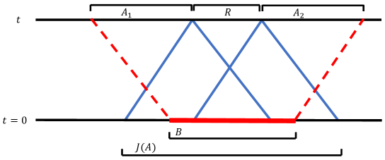
Figure 10: For any $B$ in $J(R)$ such that $R$ is in the light-cone of $B$, we can construct $A_{1},A_{2}$ such that $K(R)\equiv D(A_{1}RA_{2})\cap J(R)=B$. Then if $G(R,B,t)$ does not agree with (45), then using (27), we see that the resulting $S_{2}^{(A_{1}A_{2})}(t)$ will deviate from (47)–(48), and thus from the holographic expression.

III.3 Random void distribution and maximal entanglement growth

Consider a region $A=A_{1}\cdots A_{n}$ consisting of $n$ intervals $A_{1}=[l_{1},r_{1}],\cdots,A_{n}=[l_{n},r_{n}]$, separated by intervals $R_{1},...,R_{n-1}$, as in Fig. 7. The entanglement entropy $S_{2}^{(A)}$ can be calculated using the partition function method, and is discussed in detail in Appendix A.3. The result can be written as

$$S_{2}^{(A)}(t)={s_{\rm eq}}~{}\min_{\{\gamma\}(t)}\bigg{[}n_{\gamma}t+\sum_{\{l_{i},r_{j}\}\in\gamma}|l_{i}-r_{j}|\bigg{]}$$ (49)

where the set $\{\gamma\}(t)$ and $n_{{\gamma}}$ are defined as follows. Call any pair of left and right endpoints $\{l_{i},r_{j}\}$ from the set of all endpoints $\{l_{1},r_{1},...,l_{n},r_{n}\}$ a connectable pair at time $t$ if $t>|l_{i}-r_{j}|/2$. We can then group together the elements of $\{l_{1},r_{1},...,l_{n},r_{n}\}$ into different configurations such that every element is either unconnected to any other point, or part of one connected pair. Only connectable pairs can be connected. $\{\gamma\}(t)$ is the set of all such configurations $\gamma$ at time $t$, and $n_{\gamma}$ is the number of unconnected points in the configuration $\gamma$. Each connected pair $\{l_{i},r_{j}\}$ in a configuration $\gamma$ contributes $|l_{i}-r_{j}|$, while each unconnected point contributes $t$, so that we get (49).

Extending our discussion in section III.2 for two intervals, one can show that the same expression (49) follows by using only the following elements: (i) sharp light-cone growth; (ii) the random void distribution (44) for all initial operators; (iii) large $q$. The derivation is given in Appendix B.

The expression (49) can also be shown to be equivalent to the expression of entanglement entropy (in a scaling regime) for holographic systems after a quench. Holographic systems are a certain class of strongly coupled $(1+1)$-dimensional conformal field theories (CFT) which have a gravity dual. In the large central charge limit, their entanglement entropy can be calculated using classical gravity. More explicitly, in the regime with $t,|A_{1}|,\cdots,|A_{n}|,|R_{1}|,\cdots,|R_{n-1}|$ large while $|A_{i}|/t,|R_{i}|/t$ are fixed, the holographic entanglement entropy after a global quench has the following form (see e.g. hong_mark )

$$S_{\rm hol}(t)=\min\limits_{\sigma}~{}\bigg{[}\sum_{i=1}^{n}S_{\text{interval}}(t,|l_{i}-r_{\sigma(i)}|)\bigg{]}$$ (50)

where

$$S_{\text{interval}}(t,R)=\begin{cases}2{s_{\rm eq}}t&t<{R\over 2}\\ {s_{\rm eq}}R&t\geq{R\over 2}\end{cases}$$ (51)

and $\sigma$ are permutations of $\{1,...,n\}$, and ${s_{\rm eq}}$ is the equilibrium entropy density. The contribution we get from a permutation $\sigma$ at time $t$ on the right-hand side of (50) is equal to the contribution we get on the RHS of (49) from a configuration $\gamma(\sigma)$ where we first pair each $l_{i}$ with $r_{\sigma(i)}$, and then connect $l_{i}$ and $r_{\sigma(i)}$ if they are connectable. The set of $\gamma(\sigma)$ for all $\sigma$ at time $t$ is a subset of $\{\gamma\}(t)$ defined below (49). We can obtain the full set $\{\gamma\}(t)$ if for each choice of $\sigma$, in addition to $\gamma(\sigma)$, we include configurations where any number of the connectable pairs of the type $\{l_{i},r_{\sigma(i)}\}$ are not connected. But disconnecting a pair of connected points in a configuration while leaving other points unchanged always increases the contribution from that configuration in (49), so any element in $\{\gamma\}(t)$ which cannot be obtained as $\gamma(\sigma)$ for any $\sigma$ at time $t$ gives a larger contribution than some $\gamma(\sigma)$. Thus, the minimum value in (49) is the same as the minimum in (50).

We can check that a minimal configuration in (49) only involves connections between adjacent endpoints. So we get the same result if we restrict the definition of connectable points below (49) to adjacent endpoints $l_{i}$ and $r_{j}$ such that $t>|l_{i}-r_{j}|/2$.

As the number of intervals increases, equation (50) (or equivalently (49)) gives rise to intricate patterns of time-dependence when the relative sizes of the intervals $|A_{i}|$ and their separations $|R_{i}|$ are varied. It is remarkable that these patterns can be reproduced by the extremely simple underlying rules of sharp light-cone growth and the random void distribution. We note, however, that while for the random unitary circuits, $S_{2}$ coincides with the von Neumann entropy in the large $q$ limit, this is no indication that this is true for holographic systems in the large $c$ limit. So the entanglement spectrum of holographic systems cannot be fully approximated by random unitary circuits, and while it is natural to expect that the random void distribution should play some role in holographic systems, it cannot be the full story.

In hong_mark , it was shown using the strong subadditivity condition that the holographic expression (50) in fact maximizes the entanglement growth for an arbitrary number of intervals among all $(1+1)$-dimensional systems with a strict light cone. Thus we find that the random void distribution (44) together with sharp light-cone growth maximizes entanglement growth (recall that $S_{2}$ is upper-bounded by the von Neumann entropy). In the two-interval case, this statement implies that any system with $S_{2}(t)$ not equal to the holographic result must have $S_{2}(t)$ smaller than (47) and (48). Using  (27), this implies that

$$G(A,B;t)\geq G_{\text{RVD}}(A,B;t)$$ (52)

where $G_{\text{RVD}}(A,B;t)$ is the random void distribution (RVD) expression (45).

IV Void formation in two Clifford circuit models

As contrasts to the random void distribution, we now consider the void formation structure of two other examples of unitary circuits: (i) a free propagating model in which entanglement can only be spread, but not created, which may thus be considered a proxy for free theories; (ii) a circuit built from perfect tensors, which may be considered a model for interacting integrable systems, as while it can generate entanglement in certain initial product states, like all Clifford circuits it does not lead to growth of operator entanglement, and also does not have the form of the out-of-time-ordered correlator (OTOC) expected in chaotic systems frank ; nahum1 . Both models are special examples of Clifford circuits c1 ; c2 ; c3 , a class of unitary circuits where under time evolution, a basis operator ${{\mathcal{O}}}_{\alpha}$ transitions to another basis operator.

More explicitly, consider a unitary circuit defined by (37)–(38) and Fig. 8, where now each $U^{i,i+1}_{t}=\tilde{U}$, and $\tilde{U}$ is a (fixed) unitary matrix that evolves each basis operator in ${{\mathcal{G}}}_{i}\otimes{{\mathcal{G}}}_{i+1}$ to some basis operator. Under this time-evolution, for a given ${{\mathcal{O}}}_{\alpha}$, $c_{\alpha}^{\;\beta}(t)=1$ for a single $\beta$, and $c_{\alpha}^{\;\beta^{\prime}}(t)=0$ for all $\beta^{\prime}\neq\beta$. Since the evolution is unitary, there is a one-to-one mapping from initial operators ${{\mathcal{O}}}_{\alpha}$ to final operators ${{\mathcal{O}}}_{\beta}$.

To study entanglement growth, now instead of generic homogeneous pure product states, we have to consider a more restricted set, as these Clifford circuit models do not generate entanglement in an arbitrary initial pure product state. Furthermore, initial basis operators in the entire system can in general both grow and decrease in size under the action of the circuit $U$. The set of initial states we look at are again of the form

$$\rho_{0}=\frac{1}{q^{L}}\sum_{a\in I}{{\mathcal{O}}}_{\alpha}$$ (53)

where the set $I$ consists of $q^{L}$ basis operators, which are in general no longer just tensor products of powers of $Z_{i}$. In each of the models, we will choose $\rho_{0}$ such that the end points of all basis operators in the associated $I$ move outwards with $v=1$ under time-evolution.

As before, the entanglement growth can be obtained from (12)–(16). Note that for Clifford circuits the off-diagonal terms in (13) vanish identically due to the one-to-one mapping between initial and final basis operators. The sharp light-cone growth of operators in $I$ again implies that $S_{2}^{(A)}(t)$ is given by (20) for a single interval.

In Clifford circuits, we cannot have a void distribution like in (44) for individual initial operators ${{\mathcal{O}}}_{\alpha}$, as the probability of going to any final operator is either $0$ or $1$. Thus the functions $N_{A}(t)$, $N(A,B;t)$ and $G(A,B;t)$ defined in (14)–(16) are now the numbers (rather than the expectation values of the numbers) of initial operators in $I$ satisfying a given property. It is instructive to contrast void formation functions $G(A,B;t)$ in these models with those from the random void distribution, and see how they lead to different entanglement growth.

Before discussing the models explicitly, here we summarize some common features, which are also shared by random unitary circuits in the large $q$ limit:

1. While their void formation structure is very different from the random void distribution, we will see the corresponding void formation functions nevertheless satisfy the unitarity constraints (23) and (32)–(34).

2. The unitarity constraint (23) is satisfied in the following way. At $t>|A|/2$, take any of the $q^{2t-|A|}$ basis operators in $I\cap X(A)$, say $\tilde{{{\mathcal{O}}}}$, where $X(A)$ is the region of length $2t-|A|$ in the center of $J(A)$ (shown in Fig. 4). Defining $\tilde{I}$ as the set of all initial basis operators in $I\cap J(A)$ which are equal to $\tilde{{\mathcal{O}}}$ in $X(A)$, one finds that

   $$\sum_{\alpha\in\tilde{I},~{}\beta\text{ trivial in }A}{|c_{{\alpha}}^{\;{\beta}}(t)|^{2}}=1\ .$$ (54)

   In the Clifford circuits, we can interpret this as the fact that any choice of initial operator within the region $X(A)$ is consistent with evolving to a final operator which is equal to the identity in $A$. Since the total number of operators in $I\cap X(A)$ is equal to $q^{2t-|A|}=G(A,J(A);t)$, this also means that when we fix the part of the initial operator within $X(A)$, the initial operator in the entire region $J(A)$ which can evolve to the identity is fully determined.

   It is tempting to speculate that given sharp light-cone growth, equation (54) is true in all unitary systems.

IV.1 Free propagation model

In this model, the two-site unitary matrices in the circuit are given by hong_mark

$$\tilde{U}_{a_{1}a_{2},b_{1}b_{2}}={{\delta}}_{a_{1}b_{2}}{{\delta}}_{a_{2}b_{1}}$$ (55)

which is a discrete version of the quasiparticle models for entanglement growth proposed in calabrese . $\tilde{U}$ takes a product state to a product state at all times, but can spread the entanglement to large distances if we consider an initial state

$$\begin{gathered}\ket{\psi_{0}}=...\otimes(\frac{1}{\sqrt{q}}\sum_{n=0}^{q-1}\ket{n}_{0}\otimes\ket{n}_{1})\otimes(\frac{1}{\sqrt{q}}\sum_{n^{\prime}=0}^{q-1}\ket{n^{\prime}}_{2}\otimes\ket{n^{\prime}}_{3})...\end{gathered}$$ (56)

which has short-range entanglement between adjacent pairs of sites.

The evolution of basis operators in this model has a simple form: the basis operators at different sites evolve independently from each other, and all operators that are initially at an even (odd) site move to the right (left) at speed 1, so that at an odd time $t$, for an initial operator ${{\mathcal{O}}}\equiv\otimes_{i}O_{i}$,

$${{\mathcal{O}}}(t)=\otimes_{i=\text{even}}O_{i+t}\otimes_{i=\text{odd}}O_{i-t}$$ (57)

The density matrix for (56) is of the form (53), with $I$ the set of operators which can have any basis operator $O_{i}$ at an even site $i$, but at site $i+1$ have some fixed $\tilde{O}_{i+1}$ determined by $O_{i}$. For example, if $O_{i}=X^{m}Z^{n}$, then $\tilde{O}_{i+1}=X^{m}Z^{q-n}$. The time evolution of basis operators in $I$ can be readily obtained from (57), see Fig. 11 for an illustration.

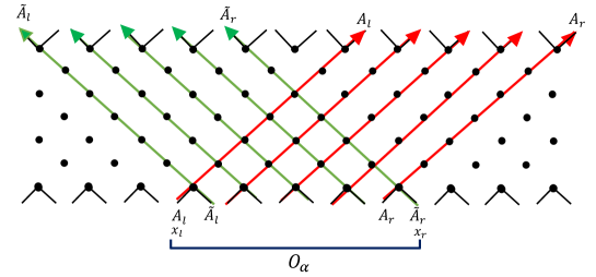
Figure 11: Growth of an operator ${{\mathcal{O}}}_{\alpha}$ in $I$. Any operator in $I$ has its left endpoint at an even site $x_{l}$ and its right endpoint at an odd site $x_{r}$. The evolution of operators follows (57) with operators at even (odd) sites moving right (left), which are shown respectively using red and green. At time $t$, the left and right endpoints are at $x_{l}-(t-1)$ and $x_{r}+(t-1)$ respectively (for sufficiently large times we have $t-1\approx t$). The resulting operator has a central void of length $2t-L_{i}$, where $L_{i}$ is the length of the initial operator, as well as other voids of length $1$. The number of sites with non-trivial operators remains fixed as a function of time.

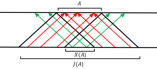
Figure 12: All operators from the region $X(A)$ propagate to $\bar{A}$. Any operator non-trivial in
$J(A)-X(A)$ has a part that propagates to $A$.

In Fig. 12, we see that all initial operators from sites in $X(A)$ propagate to $\bar{A}$ at time $t$, while operators on sites in the region $J(A)-X(A)$ propagate to $A$. An operator ${{\mathcal{O}}}_{\alpha}$ in $I$ becomes trivial in $A$ if and only if it is of the form ${{\mathcal{O}}}_{\alpha}=\tilde{O}_{X(A)}\otimes\mathbf{1}_{J(A)-X(A)}$, where $\tilde{O}_{X(A)}$ can be any operator in $I\cap X(A)$. Thus the statements (23) and (54) are both true in this model.

Now look at the form of $G(A,B;t)$. Since any initial operator in $J(A)\cap I$ that becomes trivial in $A$ must be contained within $X(A)$, the number of basis operators in $I$ contained in a subset $B$ of $J(A)$ that develop a void in $A$ is given by

$$G_{\rm free}(A,B;t)=q^{|B\cap X(A)|}\ .$$ (58)

Note that this is very different from the form (45) from the random void distribution. In particular, while (45) depends only on the length of $B$ and not on its position in $J(A)$, (58) is sensitively dependent on the position of $B$ in $J(A)$. Moreover, equation (58) can be greater than $1$ when $|B|<2|A|$, if $B$ has some overlap with $X(A)$. When applied to the entanglement entropy for two intervals using (27), such behavior can lead to $S_{2}^{(A)}(t)$ behaving non-monotonically in time, whereas (47)–(48) are non-decreasing.

One can also see that, as anticipated from (52), the expression (58) is always greater than (45)

$$G_{\text{free}}(A,B;t)\geq G_{\text{RVD}}(A,B;t),\quad\forall A,B\ .$$ (59)

Equation (59) is equivalent to $|B\cap X(A)|\geq|B|-2|A|$, which is always true as $|B|-|B\cap X(A)|\leq J(A)-X(A)=2|A|$ (see Fig. 12). It can also be checked the constraints (32)–(34) obtained from unitarity are satisfied in this model.

IV.2 Perfect tensor model

In this model, which was previously considered in qi , the Hilbert space at each site has dimension $3$ ($q$ below should be understood as being $3$), with a basis $\{\ket{0},\ket{1},\ket{2}\}$, and $\tilde{U}^{\dagger}$ acts on the Hilbert space as:

$$\tilde{U}^{\dagger}\ket{i}\otimes\ket{j}=\ket{-i-j}\otimes\ket{j-i},$$ (60)

with addition defined modulo 3. $\tilde{U}$ is a perfect tensor, that is, any balanced bipartition of its indices into inputs and outputs gives a unitary transformation. The perfect tensor model does not generate entanglement in every initial pure product state: for example, states $...\ket{0}\otimes\ket{0}...$ and $...\ket{\psi_{3}}\otimes\ket{\psi_{3}}...$ remain invariant under the action of $U$. We will consider an initial state of the form

$$\ket{\psi}=...\otimes\ket{\psi_{3}}_{0}\otimes\ket{0}_{1}\otimes\ket{\psi_{3}}_{2}\otimes\ket{0}_{3}...$$ (61)

where $\ket{\psi_{3}}\equiv\frac{1}{\sqrt{3}}\sum_{k=0}^{2}\ket{k}$, for which $I$ is the set of basis operators with powers of $X$ on even sites and powers of $Z$ on odd sites.

From (60) one finds that acting on operators in the basis (5), $\tilde{U}$ sends any basis operator on two sites to another basis operator,

$$\tilde{U}^{\dagger}(b_{1}\otimes b_{2})\tilde{U}=b^{\prime}_{1}\otimes b^{\prime}_{2},$$ (62)

and has the following properties:

1. It takes any operator with a power of $X$ on site $i$ and a power of $Z$ on site $i+1$ to an operator which is non-trivial on both $i$ and $i+1$.

2. It takes any basis operator non-trivial on a single site to a basis operator non-trivial on both sites.

3. If we know any two of $b_{1},b_{2},b^{\prime}_{1},b^{\prime}_{2}$, the other two are fully determined.

4. For $b_{1}\otimes b_{2}$ of the form $X^{m}\otimes Z^{n}$, the set of $b_{1}^{\prime}$ runs over all one-site basis operators and if we fix $b_{1}^{\prime}$, then $b_{2}^{\prime}$, $b_{1}$ and $b_{2}$ are uniquely determined (and similarly if we fix $b_{2}^{\prime}$, $b_{1}^{\prime}$, $b_{1}$ and $b_{2}$ are uniquely determined).

From items (1) and (2), we see that all operators in $I$ grow outwards with speed 1, as illustrated in Fig. 13. Thus we have the same form of $S^{(A)}_{2}(t)$ for a single interval $A$ as we found in the random circuit and free propagation models with the initial states we considered there. Note that (61) is a product state, so unlike the free propagation model, the perfect tensor model can generate entanglement in an initial pure product state.

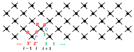
Figure 13: Sharp light-cone growth of operators in the perfect tensor model. The unitary $\tilde{U}$ at point $P$ in the circuit acts on operators at $i-1$, $i$, and gives some operator which is nontrivial on both $i-1$ and $i$. In the figure, $X^{\ast},Z^{\ast}$ refer to any powers of $X$ and $Z$, and $B$ to any non-trivial operator. $\tilde{U}$ at $Q$ acts on an operator which is non-trivial on site $i$ and trivial on site $i+1$, giving an operator which is non-trivial on both $i$ and $i+1$. By repeatedly using the fact that operators nontrivial on a single site evolve to operators non-trivial on two sites, we see that the right endpoint moves to $i+(t-1)$ at time $t$.

From items (3) and (4), one can show that for any basis operator ${{\mathcal{O}}}_{\alpha}=P_{X(A)}\otimes Q_{J(A)-X(A)}\in J(A)\cap I$, for ${{\mathcal{O}}}_{\alpha}(t)$ to be $\mathbf{1}$ in the region $A$, $P_{X(A)}$ can be any operator in $I\cap X(A)$, and if we fix $P_{X(A)}$, then ${Q}_{J(A)-X}$ is uniquely fixed. The basic idea is illustrated in Fig. 14. This implies (54), and also implies (23) as $G(A,J(A),t)$ is equal to the number of basis operators in $I\cap X(A)$, which is $q^{2t-|A|}$. Note that an initial operator that becomes trivial in $A$ at time $t$ will in general be non-trivial in the region $J(A)-X(A)$, unlike in the free propagation model.

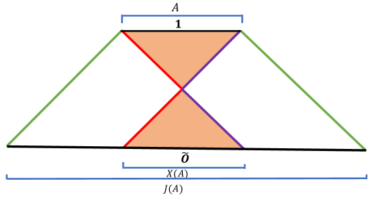
Figure 14: From causality the operators in the past domain dependence of $A$ and future domain dependence of $X(A)$ are fixed by operators in $A$ and $X(A)$ respectively. From the two “Cauchy surfaces”, shown in red and purple, which bound the regions of determined operators, by repeatedly using items (3) and (4) one can uniquely determine the all other operators in the portion of the circuits between the green lines, including the remaining parts of the initial operator in $J(A)$.

Further differences from the free propagation model can be seen by looking at the time-evolution of single initial operators in Fig. 15. The void formation in this model has a fractal structure, similar to the fractal Clifford circuits discussed in c2 ; c3 . The number of non-trivial operators in $J^{+}(O_{\alpha})$ grows unboundedly with time, in contrast to the situation in the free propagation model shown in Fig. 11.

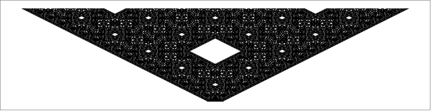
Figure 15: In the top figure, we show the time-evolution of an initial operator from $I$ which is non-trivial on one site in the perfect tensor model. In the bottom figure, we show the time-evolution of an operator non-trivial on 40 sites. Time increases in the upward direction, and the time-evolved operator has non-trivial support on black sites, and the identity operator on white sites. It is evident from the examples that for fixed time, fewer voids are formed in the case where the initial operator is bigger.

We do not have a closed form for the void formation function $G(A,B;t)$ for a general region $B$, but one can readily check in examples that (52) is satisfied. See Fig. 16. We do not have a general derivation of the constraints (32)-(34) in this model, but we have checked in a number of examples that they are obeyed.

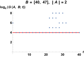
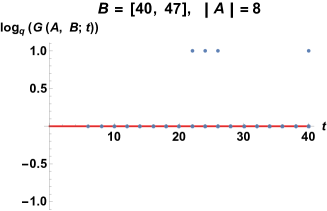
Figure 16: We consider a system with $L=80$, and sites labelled from $x=0$ to $x=79$. We fix the region $B=[40,47]$, and look at $G(A,B;t)$ for different choices of $A$. We consider intervals with $|A|=2<|B|/2$ on the left, and $|A|=8>|B|/2$ on the right, and in both cases we sample over a large number of intervals $A$ and show $\log_{q}(G(A,B;t))$ as a function of time in a single plot with the blue data points. The value expected from the random void distribution (45) is $4$ in the first case, and $0$ in the second case. We see clearly that $G(A,B;t)\geq G_{\text{RVD}}(A,B;t)$, and there are cases where $G(A,B;t)>G_{\text{RVD}}(A,B;t)$.

V Conclusions and discussion

In this paper, we examined the implications of void formation in operator evolution for entanglement growth, and showed that it plays an important role in maintaining unitarity of entanglement growth and generation of mutual information and multi-partite entanglement. We showed that the void formation probability for generic operators in random unitarity circuits is given by the random void distribution (44). We also showed that the intricate time-dependence of holographic entanglement entropies for an arbitrary number of intervals after a global quench can be understood as a consequence of the very simple rules of sharp light-cone growth and the random void distribution.

Furthermore, we found sharp differences between the void formation properties of random unitary circuits and the non-chaotic circuit models we studied, which suggests that void formation can be used to characterize differences in the operator evolution of chaotic and integrable systems which are not captured by the movement of the operator endpoints alone Kem . It is also an interesting question whether void distribution can be used to distinguish between different classes of chaotic systems. For example, it is conceivable that the random void distribution may only apply to highly chaotic systems.

In our discussion, for simplicity of presentation we have restricted to systems with sharp light-cone growth in the evolution of operators. In general systems, the fronts of operator growth should follow a distribution. For example, in random unitary circuits at finite $q$, the evolution of an operator exhibits a diffusive front around a butterfly velocity $v_{B}$ which is smaller than the lightcone velocity $v_{c}$ nahum1 ; frank . Our discussion, including the random void distribution, can be generalized to these situations, although the story is technically more complicated and will be presented elsewhere.

In our discussion we have focused on the second Renyi entropy, which can be conveniently expressed in terms of the expected number of operators that develop a void in a certain region. It would be interesting to explore the implications of void formation in operator growth for higher Renyi and von Neumann entropies, as well as whether the unitarity of these quantities imposes further constraints on void formation. It is possible these quantities will involve other aspects of void formation, and not just the squared absolute values of the operator-spreading coefficients.

While we have restricted to one spatial dimension, our discussion can be immediately generalized to higher dimensions. In one dimension, a process of void formation separates both the original operator and the full space into disconnected parts. Thus it simultaneously creates “holes” in an operator and breaks it into disjoint pieces. This is not true in higher dimensions, where “hole formation” in an operator and breaking an operator apart are distinct void formation processes, as discussed in Fig. 2. In particular, it is the latter type of process which contributes to mutual information and multi-partite entanglement among disjoint regions. It is also a natural question whether the “hole formation” and “breaking apart” could follow different probability distributions in higher dimensions.

In this paper, we defined a void as a region of identity operators among regions of nontrivial support of an operator. This definition is only appropriate for a lattice system with a finite one-site Hilbert space at infinite temperature. For finite temperature or continuum systems, a mathematically rigorous definition is tricky. Operationally, one can define a void as the part of an operator which is given by the equilibrium density operator.

It would be interesting to explore the implications of void formation for other observables to see how it affects their behavior in integrable and chaotic systems, and also to see if the non-unitarity in the absence of void formation manifests itself in other observables. For example, one can show that in some simple models without void formation, the out-of-time-ordered correlation functions (OTOCs) will also violate unitarity, although the violation appears less dramatic than that in the entanglement entropy. We will leave the exploration of this question for elsewhere.

It is important to see whether one can find other measures to characterize void formation besides than the probability functions we discussed in this paper. For example, how does one characterize the fractal structure of Fig. 15? A related question is whether such fractal structure is generic among interacting integrable systems.

Acknowledgements

We would like to thank Netta Engelhardt, Paolo Glorioso, Aram Harrow, Lampros Lamprou, Sam Leutheusser, Raghu Mahajan, Juan Maldacena, Márk Mezei, Adam Nahum, Tibor Rakovszky, Jan Zaanen and Ying Zhao for discussions. This work is supported by the Office of High Energy Physics of U.S. Department of Energy under grant Contract Number DE-SC0012567.

Appendix A Derivations in the random unitary circuits

In this Appendix, we first briefly review the partition function method introduced in nahum1 ; frank ; nahum2 for calculating various observables in random unitary circuits, and then use it to derive the random void distribution (44) and the time evolution of entanglement entropy.

A.1 Mapping to a classical Ising partition function

Consider the operator spreading coefficient ${|c_{{\alpha}}^{\;{\beta}}(t)|^{2}}$ introduced in (7), which can be written as a matrix element on four copies of the Hilbert space:

$${|c_{{\alpha}}^{\;{\beta}}(t)|^{2}} =\left|\frac{1}{q^{L}}\text{Tr}\left({{\mathcal{O}}}_{\beta}^{\dagger}U^{\dagger}{{\mathcal{O}}}_{\alpha}U\right)\right|^{2}$$ (63)

$$={1\over q^{2L}}({{\mathcal{O}}}_{\alpha})_{b_{1}a_{1}}({{\mathcal{O}}}_{\alpha}^{\dagger})_{d_{1}c_{1}}U_{a_{1}a_{2}}U^{*}_{b_{1}b_{2}}U_{c_{1}c_{2}}U^{*}_{d_{1}d_{2}}({{\mathcal{O}}}_{\beta}^{\dagger})_{a_{1}b_{1}}({{\mathcal{O}}}_{\beta})_{c_{1}d_{2}}$$

$$=\bra{{{{\mathcal{O}}}_{\alpha}}_{\uparrow}}~{}(U\otimes U^{\ast}\otimes U\otimes U^{\ast})~{}\ket{{{{\mathcal{O}}}_{\beta}}_{\uparrow}}\ .$$

In the last line we have introduced, for any operator ${{\mathcal{O}}}$ in the system, “up” and “down” spin states on four copies of $\mathcal{H}$,

$$\braket{abcd\mid{{\mathcal{O}}}_{\uparrow}}=\frac{{{\mathcal{O}}}^{\dagger}_{ab}{{\mathcal{O}}}_{cd}}{\text{Tr}[{{\mathcal{O}}}{{\mathcal{O}}}^{\dagger}]},~{}~{}~{}~{}~{}\braket{abcd\mid{{\mathcal{O}}}_{\downarrow}}=\frac{{{\mathcal{O}}}^{\dagger}_{ad}{{\mathcal{O}}}_{cb}}{\text{Tr}[{{\mathcal{O}}}{{\mathcal{O}}}^{\dagger}]}.$$ (64)

In the case where ${{\mathcal{O}}}=\mathbf{1}$, we use the notation $\ket{\uparrow}=\ket{\mathbf{1}_{\uparrow}},\ket{\downarrow}=\ket{\mathbf{1}_{\downarrow}}$.

The time evolution operator $U$ for the entire system is a tensor product of random unitaries from the Haar ensemble applied at each time on pairs of sites, as shown in (37)–(38) and Fig. 8. As explained in nahum1 ; frank ; nahum2 , after averaging over local unitaries with the Haar measure, one can express (63) as a partition function of classical Ising spins on a triangular lattice, as shown in Fig. 17, with the following specifications:

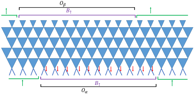
Figure 17: We show the lattice for the partition function corresponding to (63) for a particular choice of $O_{\alpha}$ and $O_{\beta}$, both without voids, and $t=5$. The boundary conditions, and the spins in the bulk fixed by the boundary conditions through the rules in Fig. 18, are shown explicitly. The remaining spins can be either up or down.

1. The top layer of the lattice corresponds to time $t$ and the bottom layer to $t=0$. They are determined respectively by $\ket{{{{\mathcal{O}}}_{\beta}}_{\uparrow}}$ and $\ket{{{{\mathcal{O}}}_{{\alpha}}}_{\uparrow}}$. If ${{\mathcal{O}}}_{\alpha}=\otimes_{i}O_{i}$, then the spins on the lower boundary are given by $O_{i\uparrow}$ at site $i$. $O_{\beta}$ similarly fixes the spins on the top boundary.

2. One can see that the interactions along the boundaries are the same for all nontrivial operators, so we can represent any nontrivial operator on the boundaries as $B_{\uparrow}$. The rules along the bottom and top boundaries are shown in Fig. 18 and  19.

3. Lattice points in the bulk of the lattice correspond to locations of local unitaries in Fig. 8, and on each lattice point lies a spin taking value ${\uparrow}$ or ${\downarrow}$. The interactions among spins in the bulk are specified by the rules of Fig. 20.

4. The partition function is obtained by summing over all possible configurations of bulk spins, and the weight of a given configuration in the partition function is obtained by multiplying the contributions from each interaction vertices in the bulk and along the boundaries.

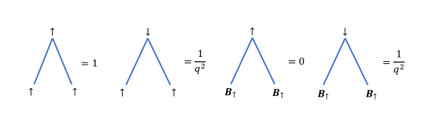
Figure 18: Rules for interactions along the bottom boundary.

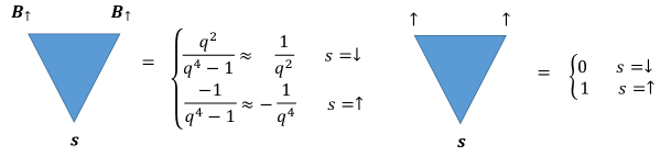
Figure 19: Rules for interactions along the top boundary.

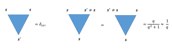
Figure 20: Interactions among the bulk spins, with $s,s^{\prime}$ taking values in $\uparrow,\downarrow$. These rules will also apply to the interactions along the top boundary for observables in Appendix A.2 and A.3.

A.2 Derivation of the random void distribution

Now let us consider the probability $P_{{{\mathcal{O}}}_{\alpha}}^{(A)}(t)=\sum_{{\beta}\;\text{with void $A$}}{|c_{{\alpha}}^{\;{\beta}}(t)|^{2}}$ for a basis operator ${{\mathcal{O}}}_{\alpha}$ to develop a void in region $A=A_{1}\cdots A_{n}$ in random unitary circuits in the large $q$ limit. We will take $A$ to be in the future light cone of ${{\mathcal{O}}}^{\alpha}$, as otherwise $P_{{{\mathcal{O}}}_{\alpha}}^{(A)}(t)$ is automatically zero.

To find $P_{{{\mathcal{O}}}_{\alpha}}^{(A)}(t)$, it is convenient to consider a slightly different quantity

$$Q_{{\alpha}}^{(\bar{A})}(t)=\sum_{{\beta}\in\bar{A}}{|c_{{\alpha}}^{\;{\beta}}(t)|^{2}}\geq P_{{{\mathcal{O}}}_{\alpha}}^{(A)}(t)$$ (65)

which also includes possible contributions from processes in which ${{\mathcal{O}}}_{\alpha}$ evolves to operators trivial in some disconnected parts of $\bar{A}$. Such contributions are not in $P_{{{\mathcal{O}}}_{\alpha}}^{(A)}(t)$. Summing (63) over all ${{\mathcal{O}}}_{\beta}$ which have the identity in $A$ we find

$$Q_{{\alpha}}^{(\bar{A})}(t)=q^{|\bar{A}|}\bra{{{{\mathcal{O}}}_{\alpha}}_{\uparrow}}~{}(U\otimes U^{\ast}\otimes U\otimes U^{\ast})~{}\ket{\uparrow}_{A}\ket{\downarrow}_{\bar{A}}$$ (66)

where $\ket{{\downarrow}_{\bar{A}}}=\otimes_{i\in\bar{A}}\ket{\downarrow}_{i}$ and we have used the fact that

$$\ket{\downarrow}_{i}=\frac{1}{q}\sum_{a=0}^{q^{2}-1}\ket{{O^{i}_{a}}_{\uparrow}}$$ (67)

where the sum over $a$ runs over the complete set of basis operators at site $i$. Now (66) can be calculated with a partition function with boundary conditions as shown in Fig. 21, with the interactions on the top boundary given by Fig. 20.

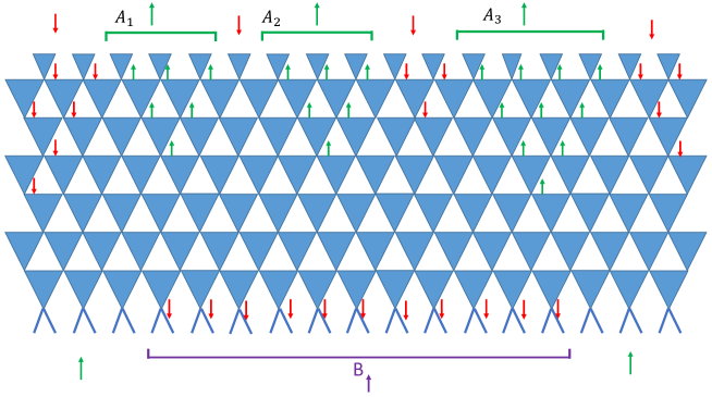
Figure 21: We show the lattice for the partition function corresponding to (66) for a case with $A$ consisting of three intervals and $t=7$. The boundary conditions, and the spins in the bulk fixed by the boundary conditions through the rules in Fig. 20 and Fig. 18, are shown explicitly. The remaining spins can be either up or down, but in the large $q$ limit we need to consider a relatively small number of configurations.

We first consider a basis operator ${{\mathcal{O}}}_{\alpha}$ with no initial voids. In the situation where there exists some $A_{i}$ for which $t<|A_{i}|/2$, the rules in Fig. 20 fix all spins in the past domain of dependence of each $A_{i}$ to be $\uparrow$ in any configuration in the partition function, while the rules in Fig. 18 fix the spins attached to ${{\mathcal{O}}}_{\alpha}$ on the lower boundary to be $\downarrow$. So we get a set of interactions like the circled interactions in Fig. 22 along the bottom boundary, and hence the contribution from any configuration to (66) is zero, and thus $P_{{{\mathcal{O}}}_{\alpha}}^{(A)}(t)=0$.

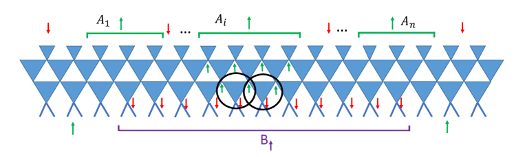
Figure 22: A case with $t<|A_{i}|/2$ for some $A_{i}$. Any configuration in the partition function at such times contributes 0 due to the circled interactions.

We now consider the situation $t>|A_{i}|/2$ for all $i$. From the rules of Fig. 20 and Fig. 18, in the large $q$ limit, the computation of the partition function corresponding to (66) reduces to finding domain walls between up and down spins: for each triangle in the lattice that a domain wall passes through, we get a factor of $\frac{1}{q}$. Starting from the top boundary, a domain wall can either reach the lower boundary or combine with another one to enclose intervals on the top boundary. A domain wall which reaches the lower boundary contributes a factor of $q^{-t}$, and the shortest domain wall which encloses an interval of length $l$ contributes $q^{-l}$ (which gives the leading contribution in the large $q$ limit).

One possible configuration contributing to (66) is shown in Fig. 23, with the domain walls between the up and down spins enclosing each of the $A_{i}$. Since all spins on the lower most bulk layer are $\downarrow$ in this configuration, we get a factor of $q^{-L}$ from the bottom boundary. The domain walls give a factor of $q^{-(|A_{1}|+...+|A_{n}|)}$. Combing these factors with the prefactor $q^{|\bar{A}|}=q^{L-(|A_{1}|+...+|A_{n}|)}$ in (66), we find the total contribution from this configuration is $q^{-2(|A_{1}|+...+|A_{n}|)}$. There are other possible domain wall configurations contributing to (66), but all these other configurations correspond to the final operators in (65) being trivial in some disconnected parts of $\bar{A}$. An example is given in Fig. 24. Thus only the configuration of Fig. 23 contributes to $P_{{{\mathcal{O}}}_{\alpha}}^{(A)}(t)$, and we conclude that

$$P_{{{\mathcal{O}}}_{\alpha}}^{(A)}(t)=q^{-2(|A_{1}|+...+|A_{n}|)}\ .$$ (68)

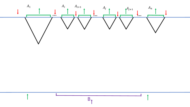
Figure 23: The configuration contributing to $P_{{{\mathcal{O}}}_{\alpha}}^{(A)}(t)$. In this plot to highlight the domain wall structure, we suppress the lattice in the bulk, only showing the domain walls between up and down spins, which are represented by the black lines.

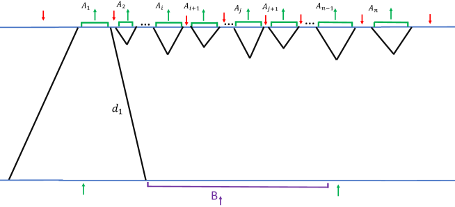
Figure 24: A domain wall configuration that contributes to (66), but not to $P_{{{\mathcal{O}}}_{\alpha}}^{(A)}(t)$. It describes processes in which ${{\mathcal{O}}}_{\alpha}$ evolves to operators trivial in the region to the left of $A_{1}$.

If ${{\mathcal{O}}}_{\alpha}$ has an initial void, then the domain wall configuration shown in Fig. 23 still exists, and evaluates to the same value. However, in this case, we also have the possibility that an initial void may evolve into a final void while the disconnected parts of the initial operator evolve independently. Such processes correspond to a new configuration in the partition function for $P_{{{\mathcal{O}}}_{\alpha}}^{(A)}(t)$, shown in Fig. 25. Clearly when either $|A|$ or $|G|$ is larger than $2t$, this is the only process which can contribute to $P_{{{\mathcal{O}}}_{\alpha}}^{(A)}(t)$. When $|G|<2t$ and $|A|<2t$, in general both possibilities exist and compete. The domain wall configuration of Fig. 23 gives the probability that the initial void closes and opens up a new void, and we have the same value as (68). The configuration of Fig. 25 gives a contribution $q^{-|A|+|G|-2t}=q^{-2|A|}q^{|A|+|G|-2t}$ which dominates when $|G|>2t-|A|$. Note that for a generic operator (42), for ${{\mathcal{O}}}_{\alpha}$ with initial void $G$, we have $|a_{\alpha}|^{2}\sim q^{-2|G|}$ and thus the overall contribution from such operators is $q^{-|A|-|G|-2t}$ which is subdominant compared with $q^{-2|A|}$ for $|A|<2t$.

To conclude this discussion, let us note that one can find the probability for an operator of size $l_{i}$ to evolve into an operator of size $l_{f}$ (assuming it is allowed by causality, and both operators do not have voids) in the large $q$ limit. This probability is independent of the initial and final operators, and is given by

$$p_{if}(t)=q^{-l_{i}-l_{f}-2t}\ .$$ (69)

From here one finds that the probability going to all final operators with length $l_{f}=l_{i}+2t$ allowed by causality is $q^{-l_{i}-l_{f}-2t}q^{2l_{f}}=q^{l_{f}-l_{i}-2t}=1$, which leads to the sharp light-cone growth noted in  (39).

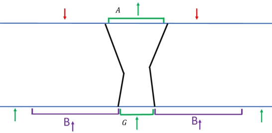
Figure 25: A domain wall configuration that contributes to $P_{{{\mathcal{O}}}_{\alpha}}^{(A)}(t)$ in the case where the initial operator ${{\mathcal{O}}}_{\alpha}$ has a single void in region $G$, and $A$ is a single interval. This configuration describes processes in which the disconnected parts of ${{\mathcal{O}}}_{\alpha}$ evolve independently to left and right of $A$. This contribution evaluates to $q^{-|A|+|G|-2t}$, and is bigger than the contribution from Fig. 23 for $t<(|G|+|A|)/2$.

A.3 Derivation of the time-evolution of $S_{2}$ in random unitary circuits with large $q$

Now let us consider the evaluation of $S_{2}^{(A)}$, which is given by (14), which we copy here for convenience

$$e^{-S_{2}^{(A)}(t)}={1\over q^{|A|}}\sum_{{\alpha}\in I}\sum_{{\beta}\in A}|c_{{\alpha}}^{\beta}(t)|^{2}\ .$$ (70)

Using  (63) and summing over all ${{\mathcal{O}}}_{\beta}$ which are the identity in $\bar{A}$ and all ${{\mathcal{O}}}_{\alpha}$ in $I$, we find

$$e^{-S_{2}^{(A)}(t)}=q^{L}{\left\langle{\rho_{0{\uparrow}}|U\otimes U^{*}\otimes U\otimes U^{*}|{\downarrow}_{A}\otimes{\uparrow}_{\bar{A}}}\right\rangle}\ .$$ (71)

In obtaining (71) we again used the fact that on summing over all operators in $A$, we obtain $\ket{{\downarrow}_{A}}$ by using (67). Also recall that $\rho_{0}=\otimes\prod_{i}\rho_{i}$ with each $\rho_{i}$ given by (10). Note that the boundary conditions at top boundary are reversed compared with (66). In the large $q$ limit, one has $e^{-\overline{S_{2}^{(A)}}(t)}=\overline{e^{-S_{2}^{(A)}(t)}}$ and all $S_{n}$ are the same nahum2 , thus the (minus) logarithm of the partition function corresponding to (71) gives $\overline{S_{2}^{(A)}}(t)$ and other entanglement entropies.

The structure of the lattice is the same as in Fig. 21, but along the top boundary, we have $\uparrow$ spins in $\bar{A}$ and $\downarrow$ spins in $A$. On the lower boundary, we have $\rho_{i\uparrow}$ at each site. As in last subsection, the evaluation of (71) boils down to summing over domain wall configurations. From the fact that each $\rho_{i}$ is a projector onto a single state in the one-site Hilbert space, we get a factor of $\frac{1}{q}$ from each site on the lower boundary, irrespective of whether the lowermost bulk layer has an $\uparrow$ or $\downarrow$ spin at that site. Thus irrespective of where the domain walls end, we get a factor of $\frac{1}{q^{L}}$ from the lower boundary, cancelling with the prefactor $q^{L}$ in (71). Effectively the bottom boundary does not play any role.

Now consider a region $A=A_{1}\cdots A_{n}$ consisting of $n$ intervals $A_{1}=[l_{1},r_{1}]$, …, $A_{n}=[l_{n},r_{n}]$, separated by intervals $R_{1},...,R_{n-1}$. Due to the boundary conditions, in each non-zero configuration in the partition function, we have $2n$ starting points of domain walls on the top boundary, from each of the $l_{i}$ and $r_{i}$. As discussed in last subsection, in the large $q$ limit, we only need to specify whether each domain wall starting on the top boundary reaches the bottom boundary, in which case we get a factor of $q^{-t}$, or joins with another domain wall to enclose an interval of length $l$, in which case we get a factor of $q^{-l}$. The latter possibility only exists for $t>l/2$.

Due to the boundary conditions, in order to separate regions of opposite spins, domain walls starting from some left-endpoint $l_{i}$ can only join with domain walls starting from some right-endpoint $r_{j}$, and from the rules of Fig. 20, domain walls cannot intersect. Let us call a pair of adjacent endpoints $l_{i}$ and $r_{j}$ an “allowed pair” at time $t$ if $|l_{i}-r_{j}|/2\leq t$. It is convenient to define a set $\{\gamma\}(t)$ of possible domain wall configurations. An element ${{\gamma}}$ of the set contains some number of “allowed pairs” $\{l_{i},r_{j}\}$ and some number of unpaired points, such that each endpoint appears exactly once. Paired points correspond to domain walls enclosing the region between them, while unpaired points correspond to domain walls reaching the bottom boundary. See Fig. 26 for an example. The contribution from a ${{\gamma}}$-configuration evaluates to $(\frac{1}{q})^{f_{\gamma}}$, where

$$f_{\gamma}=n_{\gamma}t+\sum_{\{l_{i},r_{j}\}\in\gamma}\mid l_{i}-r_{j}\mid\ ,$$ (72)

and $n_{\gamma}$ is the number of unpaired points in $\gamma$. In the large $q$ limit, the configuration with minimal $f({{\gamma}})$ dominates. We thus find

$$S^{(A)}_{2}(t)={s_{\rm eq}}\min_{\gamma}f_{{\gamma}},\quad s_{\text{eq}}=\log q\ .$$ (73)

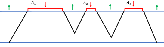
Figure 26: Example of a configuration contributing to the partition function for (71). The set $\gamma$ corresponding to this configuration is $\{l_{1},r_{3},\{l_{2},r_{1}\},\{l_{3},r_{2}\}\}$.

Appendix B Entanglement entropy from the random void distribution

Here we prove that (49) follows using only the following rules: (i) sharp light-cone growth, (ii) the random void distribution (44), (iii) large $q$, for $A$ consisting of an arbitrary number of disjoint intervals. Considering (14), we can write $N_{A}(t)$ more explicitly as

$$N_{A}(t)=N(A,D(Q);t),\quad Q=A_{1}R_{1}\cdots R_{n-1}A_{n}$$ (74)

Before presenting the proof, let us first note the two key elements which are heavily used:

1. At any given time $t$, if there exists some $|R_{i}|>2t$, the two parts of $A$ separated by interval $R_{i}$ can be independently considered. See Fig. 27 for an example, where we have a factorized form

   $$N(A,D(Q);t)=N(M_{1},D(Q_{1});t)N(M_{2},D(Q_{2});t)\ .$$ (75)

2. Consider one of the factorized parts, in which $2t$ is greater than all $R_{i}$ in that part, for example, $Q_{1}$ in Fig. 27. There are possible multiple competing contributions to $N(A_{1}A_{2},D(Q_{1});t)$, which are exhibited in Fig. 28. One contribution comes from operators which are nontrivial at all sites of $D(Q_{1})$, see Fig. 28(b), which from (44) gives

   $$N_{\text{(connected)}}^{A}(t)=M_{D(Q_{1})}(t)q^{-2|R_{1}|}=q^{|A_{1}|+|A_{2}|-|R_{1}|-2t}$$ (76)

   where $M_{D(Q_{1})}(t)=q^{|D(Q_{1})|}=q^{|A_{1}|+|A_{2}|+|R_{1}|-2t}$ is the number of initial basis operators in $D(Q_{1})$. There is also a disconnected contribution from Fig. 28(a), where nontrivial operators in $D(A_{1})$ and $D(A_{2})$ separated by an initial void evolve independently to region $A_{1}$ and $A_{2}$ respectively. Note that one may also consider initial operators with a void like in Fig. 28(c), where the non-trivial parts of the operator are not contained within $D(A_{1})$ and $D(A_{2})$. Assuming sharp light-cone growth, such an operator cannot give a disconnected contribution in which ${{\mathcal{O}}}_{1},{{\mathcal{O}}}_{2}$ evolve independently to $A_{1}$ and $A_{2}$. However, such an operator can give a connected contribution, which corresponds to situations where the initial void closes and then opens an new void. This contribution is suppressed compared to (76), as the phase space for initial operators with a void is suppressed, while the probability for an individual operator to develop a void is the same.

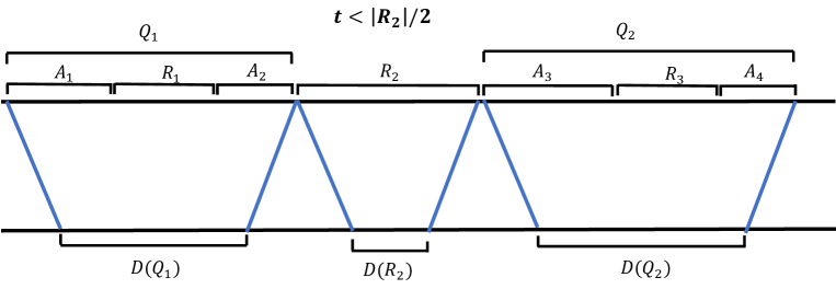
Figure 27: $R_{2}$ separates $A$ into two parts with $M_{1}=A_{1}A_{2}$ and $M_{2}=A_{3}A_{4}$, which can be independently considered. The initial operator must have identity in region $D(R_{2})$ in order to contribute to (74), and thus the contributions from two sides of region $D(R_{2})$ factorize.

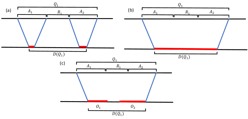
Figure 28: Possible contributions to $N(A_{1}A_{2},D(Q_{1});t)$ of Fig. 27. In the figure, red shaded regions have non-trivial operators at all sites, while the unshaded part of the initial operator is trivial.

We will prove (49) by induction. For two intervals, $n=2$, we already showed this explicitly in Sec. III.2 (the discussion leading to (47)–(48)). Here we give another derivation which connects more directly to the form (49). From item 1 above, for $t<|R|/2$,

$$N(A,D(Q),t)=N_{A_{1}}(t)N_{A_{2}}(t)\quad\to\quad S_{2}^{(A)}=S_{2}^{(A_{1})}+S_{2}^{(A_{2})}\ .$$ (77)

For $t>|R|/2$, from item 2 we have two competing contributions: the connected one, which is given by (76), and the disconnected one, given by (77). Comparing (76) and (77) in the large $q$ limit leads to the two-interval result from (49), with the connected contribution (76) corresponding to having the pair $(r_{1},l_{2})$ in the endpoint configuration $\gamma$.

Assuming we have (49) up to $n=k$ intervals, let us now consider $n=k+1$.

Let us denote the collection of $R_{i}$’s which are greater than $2t$ by ${\mathcal{R}}_{\rm big}$. Such $R_{i}$’s generate a partition ${{\mathcal{P}}}(t)$ of $A$ into $m$ parts (where $m$ can range from $1$ to $n$ depending on the time), $M_{1},...,M_{m}$. For the reason stated in Fig. 27 and item 1 above, the contribution from each $M_{i}$ factorizes, and we thus have

$$S_{2}^{(A)}(t)=\sum_{j=1}^{m}S_{2}^{(M_{j})}(t)\ .$$ (78)

The same thing happens to (49): if there exists a $|R_{i}|>2t$, then the two parts of $A$ separated by interval $R_{i}$ can be independently minimized as there are no allowed pairing between end points on the left of $R_{i}$ and those on the right of $R_{i}$. Thus equation (78) also applies to (49), and each term in the sum of (78) is given by (49) from our assumption regarding $n\leq k$.

We increase $t$ until $t=r/2$ when the set ${\mathcal{R}}_{\rm big}$ becomes empty, where $r$ is size of the largest $R_{i}$, which we call $R_{\rm max}$. Slightly before reaching $t=r/2$, from the random void distribution (44) initial operators cannot develop a void in region $R_{\rm max}$, which in the language of (49) corresponds to the fact that the two end points of $R_{\rm max}$ cannot be paired with each other. Now when $t>r/2$, from the random void distribution (44), there are new contributions coming from initial operators developing a void in region $R_{\rm max}$, which compete with previously existing ones. Note the new contributions include the connected one for the full region $D(Q)$, but also disconnected ones. See Fig. 29 for two examples. These new contributions are in one-to-one correspondence with new ${{\gamma}}$-configurations in (49) which come from pairing the two end points of $R_{\rm max}$. One can also readily check that their respective contributions agree. Thus concludes the proof.

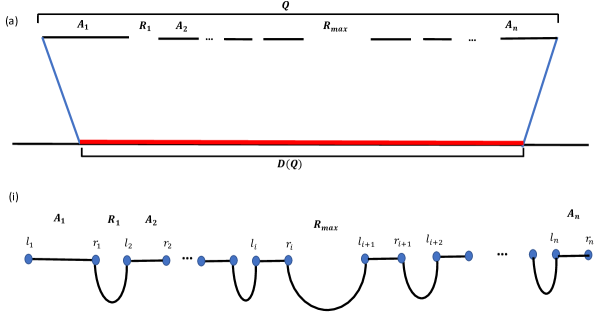
Figure 29: Two sets of initial operators contributing to (14), and the corresponding endpoint configurations $\gamma$. In (a), initial operators nontrivial everywhere in $D(Q)$ develop a void in $R\equiv R_{1}\cdots R_{n-1}$, contributing $q^{|Q|-2t}q^{-2|R|}=q^{|A|+|R|-2t}q^{-2|R|}=q^{|A|-|R|-2t}$ to $N_{A}(t)$, leading to a possible contribution $S^{(A)}_{2}(t)={s_{\rm eq}}(|R|+2t)$. We get the same contribution from $\gamma$ shown in (i), where $l_{1}$ and $r_{n}$ are the only unpaired points, and all $r_{m}$ for $m<n$ are paired with $l_{m+1}$. In (b), initial operators nontrivial everywhere in each $D(P_{i})$ go into $P_{i}$, forming voids in the $R_{j}$’s contained within the $P_{i}$’s. This contributes $q^{|P_{1}|-2t}q^{-2(|R_{1}|+...+|R_{i-2}|)}q^{|P_{2}|-2t}q^{-2|R_{\text{max}}|}q^{|P_{3}|-2t}q^{-2(|R_{i+2}|+...+|R_{n-1}|)}$ to $N_{A}(t)$, leading to a possible contribution $S^{(A)}_{2}(t)={s_{\rm eq}}(|R|-|R_{i-1}|-|R_{i+1}|+6t)$. We get the same contribution from $\gamma$ shown in (ii), where $l_{1}$, $r_{i-1}$, $l_{i}$, $r_{i+1}$, $l_{i+2}$, and $r_{n}$ are the only unpaired points, and all $r_{m}$ for $m\neq i-1,i+1,n$ are paired with $l_{m+1}$.

In the above proof, we assumed the random void distribution for all initial operators, an assumption that is not precisely true in random unitary circuits in the large $q$ limit due to the subtlety noted at the end of Appendix A.2. Yet we found by the partition function calculation of Appendix A.3 that equation (49) is true in random unitary circuits in the large $q$ limit, indicating that the cases where $P_{{{\mathcal{O}}}_{\alpha}}^{(A)}(t)$ for initial operators with voids is not given by the random void distribution can be ignored in the calculation of $S_{2}$. For instance, this means that in Fig. 28(c), the cases in random unitary circuits where the disconnected contribution (due to independent evolution of $O_{1}$ and $O_{2}$ respectively into $A_{1}$ and $A_{2}$) is dominant can be ignored. Indeed, on using (69) and counting the number of relevant initial and final operators, we can check that the collective disconnected contribution from all initial operators like in Fig. 28(c) is the same as that from Fig. 28(a), changing $S_{2}$ at most by a $q$-independent $O(1)$ term which can be neglected in the large $q$ limit.

References

- (1) D. A. Roberts, D. Stanford and L. Susskind, “Localized shocks,” JHEP 1503, 051 (2015) [arXiv:1409.8180 [hep-th]].
- (2) T. Prosen and I. Piorn, “Operator space entanglement entropy in transverse Ising chain” Phys. Rev. A 76, 032316 (2007) [arXiv:0706.2480]
- (3) I. Piorn and T. Prosen , “Operator Space Entanglement Entropy in XY Spin Chains” Phys. Rev. B 79, 184416 (2009) [arXiv:0903.2432]
- (4) J. Dubail, “Entanglement scaling of operators: a conformal field theory approach, with a glimpse of simulability of long-time dynamics in 1+1d,” arXiv:0903.2432
- (5) C. Jonay, D. A. Huse, and A. Nahum, “Coarse-grained dynamics of operator and state entanglement,” 1803.00089.
- (6) S. H. Shenker and D. Stanford, “Black holes and the butterfly effect,” JHEP 1403, 067 (2014) [arXiv:1306.0622 [hep-th]].
- (7) W. W. Ho and D. A. Abanin, “Entanglement dynamics in quantum many-body systems,” Phys. Rev. B 95, 094302 (2017); arXiv:1508.03784.
- (8) A. Nahum, S. Vijay, J. Haah, “Operator Spreading in Random Unitary Circuits,” arXiv:1705.08975.
- (9) C. von Keyserlingk, T. Rakovszky, F. Pollmann, and S. Sondhi, “Operator hydrodynamics, OTOCs, and entanglement growth in systems without conservation laws,” arXiv:1705.08910.
- (10) T. Zhou and A. Nahum, “Emergent statistical mechanics of entanglement in random unitary circuits,” arXiv:1804.09737.
- (11) H. Casini, H. Liu and M. Mezei, “Spread of entanglement and causality,” JHEP 1607, 077 (2016) [arXiv:1509.05044 [hep-th]].
- (12) Pavan Hosur, Xiao-Liang Qi, Daniel A. Roberts, and Beni Yoshida, “Chaos in quantum channels,” arXiv:1511.04021.
- (13) E. H. Lieb and D. W. Robinson, “The finite group velocity of quantum spin systems,” Commun. Math. Phys. 28 251 (1972).
- (14) D. A. Roberts and D. Stanford, “Two-dimensional conformal field theory and the butterfly effect,” Phys. Rev. Lett. 115, no. 13, 131603 (2015) [arXiv:1412.5123 [hep-th]].
- (15) M. Mezei and D. Stanford, “On entanglement spreading in chaotic systems,” JHEP 05 (2017) 065, arXiv: 1608.05101.
- (16) H. Liu and S. J. Suh, “Entanglement Tsunami: Universal Scaling in Holographic Thermalization,” Phys. Rev. Lett. 112, 011601 (2014) [arXiv:1305.7244 [hep-th]].
- (17) C. T. Asplund, A. Bernamonti, F. Galli and T. Hartman, “Entanglement Scrambling in 2d Conformal Field Theory,” arXiv:1506.03772 [hep-th].
- (18) S. Xu and B. Swingle, “Locality, Quantum Fluctuations, and Scrambling,” arXiv:1805.05376
- (19) S. Xu and B. Swingle, “Accessing scrambling using matrix product operators,” Nat. Phys. (2019) doi:10.1038/s41567-019-0712-4 [arXiv:1802.00801]
- (20) E. Leviatan, F. Pollmann, J. H. Bardarson, D. A. Huse, E. Altman, “Quantum thermalization dynamics with Matrix-Product States,” arXiv:1702.08894
- (21) S. Leichenauer and M. Moosa, “Entanglement Tsunami in (1+1)-Dimensions,” arXiv:1505.04225 [hep-th].
- (22) V. Balasubramanian, A. Bernamonti, N. Copland, B. Craps and F. Galli, Phys. Rev. D 84, 105017 (2011) [arXiv:1110.0488 [hep-th]].
- (23) D. M. Schlingemann, H. Vogts, and R. F. Werner, Journal of Mathematical Physics 49, 112104 (2008).
- (24) J. Gutschow, Applied Physics B 98, 623 (2010).
- (25) J. Gutschow, S. Uphoff, R. F. Werner, and Z. Zimboras, Journal of Mathematical Physics 51, 015203 (2010).
- (26) P. Calabrese and J. L. Cardy, “Evolution of entanglement entropy in one-dimensional systems,” J. Stat. Mech. 0504, P04010 (2005) [cond-mat/0503393].
- (27) C. T. Asplund and A. Bernamonti, Phys. Rev. D 89, no. 6, 066015 (2014) [arXiv:1311.4173 [hep-th]].
- (28) S. Gopalakrishnan, D. A. Huse, V. Khemani, and R. Vasseur, “Hydrodynamics of operator spreading and quasiparticle diffusion in interacting integrable systems,” arXiv:1809.02126.