Optimal experimental design under irreducible uncertainty for linear inverse problems governed by PDEs

Abstract

We present a method for computing A-optimal sensor placements for infinite-dimensional Bayesian linear inverse problems governed by PDEs with irreducible model uncertainties. Here, irreducible uncertainties refers to uncertainties in the model that exist in addition to the parameters in the inverse problem, and that cannot be reduced through observations. Specifically, given a statistical distribution for the model uncertainties, we compute the optimal design that minimizes the expected value of the posterior covariance trace. The expected value is discretized using Monte Carlo leading to an objective function consisting of a sum of trace operators and a binary-inducing penalty. Minimization of this objective requires a large number of PDE solves in each step. To make this problem computationally tractable, we construct a composite low-rank basis using a randomized range finder algorithm to eliminate forward and adjoint PDE solves. We also present a novel formulation of the A-optimal design objective that requires the trace of an operator in the observation rather than the parameter space. The binary structure is enforced using a weighted regularized $\ell_{0}$-sparsification approach. We present numerical results for inference of the initial condition in a subsurface flow problem with inherent uncertainty in the flow fields and in the initial times.

Keywords: Optimal design, inverse problems, model uncertainty, optimization under uncertainty, model reduction, subsurface flow.

1 Introduction

Many problems in the sciences and engineering require inference of unknown/uncertain parameters from indirect observations and a mathematical model that relates the parameters to these observations. Having access to informative data is integral to accurate parameter inference. However, the cost of data collection or physical restrictions often limit how much data one can collect. Even if one has access to large stores of data, processing large amounts of it can be expensive; moreover, data can be full of redundancies—poor experimental design choices can limit the information data contains about the parameters. A natural question to ask is: how can we design experimental conditions for data collection to optimally reconstruct/infer parameters of interest? Addressing this requires solving an optimal experimental design (OED) problem.

Inverse problems stemming from real-world applications often contain uncertainties in the governing model, in addition to the uncertain inversion parameters. We focus on irreducible model uncertainties, i.e., uncertainties that—for all practical purposes—cannot be reduced via parameter estimation. Examples of such irreducible uncertainties arise in inversion of the initial concentration of a contaminant in groundwater flow. In this problem, one usually only has rough estimates of the true groundwater velocity field. Additionally, one might not exactly know the exact time at which the contaminant has been released. Unlike uncertainties that could be reduced with observations and parameter estimation, these uncertainties are difficult to reduce. However, they should be taken into account when computing experimental designs. This article is about design of experiments for inverse problems governed by models containing such irreducible uncertainties.

We focus on infinite-dimensional Bayesian inverse problems in which the parameter-to-observable map is linear; see section 2 for a brief overview. The irreducible uncertainty may enter nonlinearly into the model and we assume some knowledge about its distribution. This knowledge could be based, for instance, on historic data, or it could be the posterior distribution obtained as the solution of another Bayesian inverse problem. To accommodate such an irreducible additional uncertainty in OED, we extend the notion of A-optimal design to A-optimal design under (irreducible) uncertainty, which we define as the design that minimizes the expected value of the average posterior variance; see section 3.

In the present work, we restrict the idea of experimental design to that of choosing locations for placing data collecting sensors, though our approach can be adapted to more general experimental design problems. We formulate the OED problem as that of finding an optimal subset of locations for sensor placement from a pre-specified network of candidate sensor locations. We assign to each candidate location a non-negative design weight indicating its importance. We seek binary designs and interpret a candidate sensor location with a design weight of $1$ as a location where a sensor should be placed. To circumvent the computational challenges of binary optimization, we relax the binary condition and add a sparsity-inducing (or binary-inducing) penalty to our optimal design objective; see section 3.3.

Literature survey and challenges. Classical references for optimal experimental design problems include [6, 32, 25, 27]. OED for inverse problems governed by computationally intensive models has been subject to intense research activity in the past couple of decades; see, e.g., [21, 16, 19, 20, 23, 4, 34, 29, 7]. Our focus is on ill-posed infinite-dimensional Bayesian linear inverse problems. We build on previous work [15, 17, 3], which developed efficient methods for computing A-optimal designs for high- or infinite-dimensional linear inverse problems using either a Bayesian or a frequentist approach. Other approaches for computing optimal experimental designs for high/infinite-dimensional linear inverse problems are explored, for example, in [24, 5, 2]. In [24], the authors propose a measure-based OED formulation that does not choose sensor locations from a finite number of candidate locations but allows sensors to be placed anywhere on a closed subset of the domain. The articles [2, 5] explore an alternate OED criterion—D-optimality—for infinite-dimensional Bayesian linear inverse problems.

We extend previous approaches by taking into account irreducible uncertainty in the model. This results in a challenging optimization under uncertainty (OUU) problem [30, 9, 22], as we now describe. In linear inverse problems, the average posterior variance of the inversion parameters—the A-optimal criterion—is defined by the trace of the posterior covariance operator $\mathcal{C}_{\!\mathrm{post}}$. This operator is high-dimensional (upon discretization), dense, and expensive-to-apply. Specifically, applying $\mathcal{C}_{\!\mathrm{post}}$ to vectors requires many PDE solves. This covariance operator is a function of the vector of experimental design weights and the random variables characterizing the model uncertainty. The resulting OED under uncertainty (OEDUU) problem is challenging, because the OEDUU objective is the expected value of $\tr\left[\mathcal{C}_{\!\mathrm{post}}\right]$, with expectation taken with respect to the model uncertainty. It is worth noting that optimizing $\tr\left[\mathcal{C}_{\!\mathrm{post}}\right]$ even for a single instance of $\mathcal{C}_{\!\mathrm{post}}$ is in itself a challenging problem [3].

As mentioned above, our goal is finding binary design vectors, which are in general difficult to compute. Our approach for this considers a relaxation of the problem and uses an adaptation of the regularized $\ell_{0}$-sparsification approach outlined in [3]. Note that there are different options to control sparsity of designs; see e.g., [11, 17, 34].

Our approach. We follow a sample average approximation (SAA) approach for the OEDUU problem, where we approximate the expectation in the OEDUU objective by sample averaging over the model uncertainty. Corresponding to each realization of the irreducible model uncertainty, we have a realization of the parameter-to-observable map (forward operator) that defines a specific instance of $\mathcal{C}_{\!\mathrm{post}}$; see section 4.1. Computing traces of these operators is challenging due to their high-dimensionality (upon discretization) and the high cost (in terms of PDE solves) of applying the covariance operators to vectors.

To mitigate the computational cost of OEDUU, we present a novel formulation of the OED criterion in the observation space. Thus, we only require computing traces of operators defined on the observation space which in many infinite-dimensional inverse problems has a smaller dimension than that of the discretized parameter space; see section 4.2. However, computing the resulting OEDUU objective and its gradient still requires many PDE solves, and these computations are repeated in each step of an optimization algorithm used for solving the OEDUU problem. Hence, it is imperative to exploit problem structure to compute low-rank approximations of the forward operator samples to eliminate frequent PDE solves from the optimization iterations. To do so, we employ randomized matrix methods to compute a low rank basis that jointly approximates the range space for all or subsets (clusters) of forward operator samples; see section 5.

We explore the effectiveness and performance of our methods for a realistic groundwater initial condition inversion problem; see sections 6–8. In this application, the (high-dimensional) irreducible uncertainties stem from: an unknown groundwater flow field (as a result of uncertainty in the subsurface permeability field), and from an uncertain observation time.

Contributions. The contributions of this article are as follows: (1) We propose a mathematical formulation for OED under irreducible model uncertainty in infinite-dimensional Bayesian linear inverse problems. (2) We present a novel OED objective formulation in the observation space that avoids trace estimation in high-dimensional discretized parameter spaces. This formulation also applies to A-optimal OED without additional model uncertainty. (3) We develop an efficient and practical reduced order modeling framework for OEDUU that eliminates PDE solves from the optimization process. (4) We present a comprehensive set of numerical experiments that illustrate the proposed approach and demonstrate its effectiveness.

Limitations. The present work also has limitations. (1) Our formulation is restricted to linear parameter-to-observation maps, Gaussian priors, and additive Gaussian noise. Further work is needed to extend it to nonlinear inverse problems. One possible extension is to use a Gaussian approximation of the posterior distribution as in [4]. (2) We use Monte Carlo sampling to approximate the irreducible uncertainty. If the aim is a highly accurate approximation of this uncertainty, a large number of samples might be needed.

2 Background

In this section, we review relevant material required for the formulation of OED problems under uncertainty for infinite-dimensional Bayesian inverse problems. We also summarize previous work which this paper builds on.

2.1 Infinite-dimensional Bayesian linear inverse problems

We begin our discussion by formulating a prototypical Bayesian linear inverse problem, which is the primary focus of the present work. A detailed treatment of general nonlinear Bayesian inverse problems can be found for instance in [13].

Given finite-dimensional observations, $\mathbf{d}\in\mathbb{R}^{d}$, we seek to infer an unknown parameter, $m$, which is related to the data through

$$\centering\mathbf{d}=\mathcal{F}m+\mathbf{\eta}.\@add@centering$$ (1)

We consider the case where $m$ is an element of an infinite-dimensional Hilbert space $\mathcal{H}$, e.g., $\mathcal{H}=L^{2}(\mathcal{D})$ with $\mathcal{D}$ being a bounded domain in $\mathbb{R}^{2}$ or $\mathbb{R}^{3}$. Here, $\mathcal{F}:\mathcal{H}\rightarrow\mathbb{R}^{d}$ is a continuous linear parameter-to-observable map (forward model). In our target applications, computing $\mathcal{F}m$ for a given $m$ involves solving a partial differential equation (PDE) followed by application of an observation operator. In (1), we assume $\mathbf{\eta}\sim\mathcal{N}(\mathbf{0},\boldsymbol{\Gamma}_{\!\mathrm{noise}})$.

Following a Bayesian approach, we model the parameter $m$ as a random variable and impose a prior probability law for $m$. The prior law is a probabilistic description of our prior knowledge about the parameter. We use a Gaussian prior $\mathcal{N}(m_{\!\mathrm{pr}},\mathcal{{C}}_{\!\mathrm{pr}})$ where the mean $m_{\!\mathrm{pr}}$ is a sufficiently regular element of $\mathcal{H}$ and the covariance operator $\mathcal{{C}}_{\!\mathrm{pr}}$ is a trace-class operator defined through the inverse of a differential operator. More precisely, we let $\mathcal{{C}}_{\!\mathrm{pr}}=\mathcal{A}^{-2}$ where $\mathcal{A}=-\rho\Delta+\delta\mathcal{I}$; here, $\Delta$ is the Laplace operator, $\delta>0$ controls the magnitude of the variance and $\rho>0$ controls the correlation length. This choice ensures that the prior covariance operator is trace-class in two and three space dimensions; see [13] for details.

The solution of the Bayesian inverse problem is the posterior probability law for the parameter, which is conditioned on measurement data. For a linear inverse problem with a Gaussian prior and an additive Gaussian noise model, which is what we assume, it is well known [13] that the posterior distribution is also Gaussian, namely $\mathcal{N}(m_{\!\mathrm{post}},\mathcal{C}_{\!\mathrm{post}})$ with

$$\mathcal{C}_{\!\mathrm{post}}=\left(\mathcal{F}^{*}{\boldsymbol{\Gamma}^{-1}_{\!\mathrm{noise}}}\mathcal{F}+\mathcal{{C}}_{\!\mathrm{pr}}^{-1}\right)^{-1}\quad\text{and}\quad m_{\!\mathrm{post}}=\mathcal{C}_{\!\mathrm{post}}\left(\mathcal{F}^{*}{\boldsymbol{\Gamma}^{-1}_{\!\mathrm{noise}}}\mathbf{d}+\mathcal{{C}}_{\!\mathrm{pr}}^{-1}m_{\!\mathrm{pr}}\right).$$ (2)

2.2 Bayesian linear inverse problem with model uncertainty

We are interested in the design of experiments for inverse problems governed by PDEs with uncertain parameters representing the irreducible uncertainty. Note that these uncertainties are in addition to the uncertainty in the inversion parameter. In such cases, the forward operator $\mathcal{F}$ is a function of uncertain parameters. We will formalize this below.

Let $(\Omega,\mathcal{G},P)$ be a probability space, where $\Omega$ is a sample space, $\mathcal{G}$ is a suitable $\sigma$-algebra on $\Omega$, and $P$ is a probability measure. We let $\xi=\xi(\omega)$ denote a random variable, defined on $(\Omega,\mathcal{G},P)$, that models the irreducible uncertainty in $\mathcal{F}$; for example, $\xi$ could be a random vector whose entries define uncertain parameters in the governing PDEs, or $\xi$ could be a function-valued random variable (i.e., a random field coefficient). In this case, the forward operator is a random variable $\mathcal{F}:\Omega\rightarrow\mathcal{L}(\mathcal{H},\mathbb{R}^{d})$, where $\mathcal{L}(\mathcal{H},\mathbb{R}^{d})$ is the space of linear transformations from $\mathcal{H}$ to $\mathbb{R}^{d}$. For each $\omega\in\Omega$, we have a realization $\mathcal{F}(\omega)=\mathcal{F}(\xi(\omega))$ of the forward model. Thus, the solution of the corresponding Bayesian linear inverse problem depends on $\xi$ and is given by $\mathcal{N}(m_{\!\mathrm{post}}(\xi),\mathcal{\mathcal{C}_{\!\mathrm{post}}}(\xi))$, with

$$\mathcal{C}_{\!\mathrm{post}}(\xi)=\left(\mathcal{F}(\xi)^{*}{\boldsymbol{\Gamma}^{-1}_{\!\mathrm{noise}}}\mathcal{F}(\xi)+\mathcal{{C}}_{\!\mathrm{pr}}^{-1}\right)^{-1}\quad\text{and}\quad m_{\!\mathrm{post}}(\xi)=\mathcal{C}_{\!\mathrm{post}}\left(\mathcal{F}(\xi)^{*}{\boldsymbol{\Gamma}^{-1}_{\!\mathrm{noise}}}\mathbf{d}+\mathcal{{C}}_{\!\mathrm{pr}}^{-1}m_{\!\mathrm{pr}}\right).$$ (3)

2.3 A-optimal design of infinite-dimensional inverse problems

We focus on A-optimal design of Bayesian linear inverse problems. That is, we seek designs (sensor placements) that result in minimized average posterior variance. In the present infinite-dimensional formulation, this amounts to minimizing the trace of $\mathcal{C}_{\!\mathrm{post}}$; see [3] for details. The additional challenge for inverse problems with uncertainties in the governing model is that the covariance operator itself depends on the random variable $\xi$ that defines the uncertain parameters in the model. In the next section, we formulate the A-optimal design problem as that of optimization under uncertainty. We refer to this problem as optimal experimental design under uncertainty (OEDUU).

3 A-optimal design of experiments for linear Bayesian inverse problems with irreducible model uncertainty

We begin with a discussion of experimental design for infinite-dimensional linear inverse problems with uncertain forward models in section 3.1. In section 3.2, we present our formulation of Bayesian A-optimality for such inverse problems, and in section 3.3, we formulate the optimization problem for finding A-optimal designs in the inverse problems under study.

3.1 Design in the Bayesian inverse problem with uncertain forward models

In OED for inverse problems we are interested in determining how to collect measurement data to optimize the parameter inference. The definition of an “experimental design” is problem specific. For example, in inverse problems in tomography, the design could correspond to choosing a subset of angles for an x-ray source to hit an object. On the other hand, in the inverse problem of identifying the source of a contaminant, the design corresponds to the placement of sensors that are used to measure the contaminant concentration.

We consider a finite generic set of candidate experiments denoted by $x_{i}\in X$, $i=1,\ldots,d$, where $X$ is a problem specific set of admissible experiments. More concretely, in the tomography example, $x_{i}$’s are measurement angles and $X$ corresponds to the set of all possible measurement angles; and in the subsurface flow example, $x_{i}$’s indicate sensor locations and $X$ is the physical domain in which the sensors can be placed. We assign a nonnegative weight $w_{i}$ to each choice of $x_{i}$. Thus, an experimental design is specified by a design vector $\mathbf{w}=(w_{1},w_{2},\ldots,w_{d})$. Ideally, we would like binary design vectors: in the case $w_{i}=1$, we will collect the measurement corresponding to $x_{i}$, and if $w_{i}=0$, the corresponding experiment will not be performed (or the data not be collected). However, an OED problem of finding binary optimal design vectors has combinatorial complexity—an extremely challenging problem. To cope with this, we relax the binary assumption on the weights and allow the weights to take values in the interval $[0,1]$. We then seek to enforce a binary structure on the computed weights using a suitable penalty method, as discussed further below.

To incorporate a generic design $\mathbf{w}$ into the Bayesian inverse problem, we define a diagonal matrix $\mathbf{W}\in\mathbb{R}^{d\times d}$, which, in a generic OED problem, contains the weights $\mathbf{w}=(w_{1},w_{2},\ldots,w_{d})$ on the diagonal. In a sensor placement problems for an inverse problem governed by a time-dependent PDE, as in the example used in section 6, the goal is to select an optimal subset of $s$ candidate sensor locations, which collect measurements at $r$ observation times. When a sensor location is chosen, we assume that it collects measurements for all $r$ observation times. In this setup, the design vector $\mathbf{w}$ has dimension $s$, and the vector of measurement data has dimension $d=sr.$ Thus, $\mathbf{W}\in\mathbb{R}^{sr\times sr}$ is a block diagonal matrix with each $s\times s$ diagonal block being a diagonal matrix with the sensor weights on the diagonal.

We incorporate the design vector $\mathbf{w}$ in the Bayesian inverse problem by considering a weighted forward operator ${\mathcal{F}}(\xi;\mathbf{w}):=\mathbf{W}^{\frac{1}{2}}\mathcal{F}(\xi)$. As before, $\xi$ is the random variable that models uncertainty in the governing PDEs. The posterior law of $m$ now depends on the design $\mathbf{w}$ as follows:

$$\mathcal{C}_{\!\mathrm{post}}(\xi,\mathbf{w})=\left({\mathcal{F}}^{*}(\xi)\mathbf{W}^{\frac{1}{2}}{\boldsymbol{\Gamma}^{-1}_{\!\mathrm{noise}}}\mathbf{W}^{\frac{1}{2}}{\mathcal{F}}(\xi)+\mathcal{{C}}_{\!\mathrm{pr}}^{-1}\right)^{-1}\quad\text{and}$$ (4)

$$m_{\!\mathrm{post}}(\xi,\mathbf{w})=\mathcal{C}_{\!\mathrm{post}}\left(\mathcal{F}(\xi)^{*}\mathbf{W}^{\frac{1}{2}}\boldsymbol{\Gamma}^{-1}_{\!\mathrm{noise}}\mathbf{d}+\mathcal{{C}}_{\!\mathrm{pr}}^{-1}m_{\!\mathrm{pr}}\right).$$

As discussed later, if the noise covariance $\boldsymbol{\Gamma}^{-1}_{\!\mathrm{noise}}$ is diagonal, the expression for the posterior covariance operator simplifies and it is not necessary to consider the square root of $\mathbf{W}$.

3.2 A-optimal design under uncertainty

We focus on A-optimal design of linear inverse problems. Following [3], for a fixed realization of $\xi$, the A-optimal design is one which minimizes the average posterior variance, i.e., the design which minimizes $\tr{\left[\mathcal{C}_{\!\mathrm{post}}(\xi,\mathbf{w})\right]}$. We extend the notion of A-optimal designs to Bayesian inverse problems with uncertain model parameters by formulating the OED problem as that of minimizing the expected value of $\tr\left[\mathcal{C}_{\!\mathrm{post}}(\xi(\omega),\mathbf{w})\right]$. Thus, the OED criterion we consider is given by

$$\phi(\mathbf{w}):=\int_{\Omega}\tr\left[\mathcal{C}_{\!\mathrm{post}}(\xi(\omega),\mathbf{w})\right]P(d\omega).$$ (5)

Note that taking the perspective of optimization under uncertainty, minimizing (5) amounts to a risk-neutral design. Other scalarization methods are possible, e.g., risk-averse objectives, which place emphasis on avoiding particularly poor designs [22, 31].

3.3 The OED Problem

An effective solution method for finding OEDs must provide the user a mechanism to strike a balance between the competing goals of minimizing posterior uncertainty and using as few sensors as possible. We address this by using a sparsifying penalty function to promote sparse (and eventually, binary) optimal design vectors. Accordingly, we formulate the optimization problem for finding an OED as follows:

$$\min_{\mathbf{w}\in[0,1]^{s}}\phi(\mathbf{w})+\gamma\psi\left(\mathbf{w}\right),$$ (6)

where $\phi(\mathbf{w})$ is the OED criterion defined in (5), $\psi:\mathbb{R}_{+}^{s}\rightarrow[0,\infty)$ is a sparsity-inducing penalty function, and $\gamma$ controls the degree of sparsity.

A simple choice for $\psi$ is the $\ell_{1}$-norm, $\psi(\mathbf{w})=\mathbf{1}^{T}\mathbf{w}$, where $\mathbf{1}$ is the vector of all ones. While using an $\ell_{1}$-norm penalty leads to sparse designs, it does not yield binary design vectors. To obtain binary designs, using an $\ell_{1}$-norm penalty can be combined with thresholding to decide where the sensors should be placed, but as numerically studied in [3], the resulting designs are suboptimal.

In the present work, we follow the regularized $\ell_{0}$-sparsification procedure introduced in [3], which typically results in binary optimal design vectors. This approach involves a continuation procedure in which a sequence of minimization problems with penalty functions that successively approximate the $\ell_{0}$-“norm” are solved. For $\mathbf{w}\in\mathbb{R}^{s}$, we denote the $\ell_{0}$-“norm” as $\|\mathbf{w}\|_{\ell_{0}}$ and define it as the number of non-zero entries in $\mathbf{w}$. The procedure is initialized with $\mathbf{w}_{\varepsilon(0)}$, which is obtained by solving (6) with an ${\ell_{1}}$ penalty. Then, at step $i$ of the continuation procedure, a new solution $\mathbf{w}_{\varepsilon(i)}$ is obtained by solving

$$\min_{\mathbf{w}\in[0,1]^{s}}{\phi}(\mathbf{w})+\gamma\psi_{\varepsilon(i)}(\mathbf{w})$$ (7)

using the previous $\mathbf{w}_{\varepsilon(i-1)}$ as an initial guess; the penalty function $\psi_{\varepsilon(i)}(\mathbf{w})$ is chosen from a family of continuously differentiable penalty functions that approach the $\ell_{0}$-“norm” as $i\rightarrow\infty$. This procedure uses non-convex functions and thus one cannot guarantee uniqueness of solutions beyond the $\ell_{1}$-norm initialization. However, numerical experiments in [3] and in section 8 show that the method performs well in practical examples.

We find that using the $\ell_{0}$ sparsification approach, there may be a large disparity between the sparsity (and the values of the objectives) for the $\ell_{1}$ solution, $\mathbf{w}_{\varepsilon(0)}$, and for the binary weight vector $\mathbf{w}_{*}$ obtained at the end of the continuation procedure. That is, for a fixed $\gamma$, we found that $\|\mathbf{w}_{\varepsilon(0)}\|_{\ell_{1}}\ll\|\mathbf{w}_{*}\|_{\ell_{0}}$. This results in the continuation procedure being rather sensitive to the choice of the sequence $\varepsilon(i)$. As a remedy, we use a rescaling to help mitigate this issue, as follows. Note we can scale the $\ell_{1}$ penalty linearly with a scaling factor $\alpha>0$ through $\|\alpha\mathbf{w}\|_{\ell_{1}}=\alpha\|\mathbf{w}\|_{\ell_{1}}$. However, this scaling has no effect on the $\ell_{0}$ norm $\|\alpha\mathbf{w}\|_{\ell_{0}}=\|\mathbf{w}\|_{\ell_{0}}$. Since the first step in the continuation strategy in [3] involves solving the minimization problem with an $\ell_{1}$ penalty to obtain $\mathbf{w}_{\varepsilon(0)}$, we can control the sparsity of $\mathbf{w}_{\varepsilon(0)}$ by using an $\alpha$-scaled $\ell_{1}$ penalty. More specifically, $\alpha\in(0,1)$ produces a less sparse initial guess for the continuation procedure than $\alpha\geq 1$. Once an initial guess $\mathbf{w}_{\varepsilon(0)}$ is obtained, we use the following family of scaled sparsity-inducing penalty functions:

$$\psi_{\varepsilon}(\alpha\mathbf{w}):=\sum_{i=1}^{s}f_{\varepsilon}(\alpha w_{i}),$$ (8)

where, for $\varepsilon>0$,

$$f_{\varepsilon}(\alpha w)=\begin{cases}\alpha w/\varepsilon\quad&\mbox{if }\hskip 8.53581ptw<\frac{\varepsilon}{2\alpha},\\ c_{3}{(\alpha w)}^{3}+c_{2}{(\alpha w)}^{2}+c_{1}(\alpha w)+c_{0}\quad&\mbox{if }\hskip 8.53581pt\frac{\varepsilon}{2\alpha}\leq w<\frac{2\varepsilon}{\alpha},\\ 1\quad&\mbox{if }\hskip 8.53581ptw\geq\frac{2\varepsilon}{\alpha};\end{cases}$$

as in [3], the constants $c_{3},c_{2},c_{1}$ and $c_{0}$ are chosen such that $f_{\varepsilon}(\alpha w)$ is continuously differentiable on $[0,1]$.

To summarize, we choose a decreasing sequence $\{\varepsilon(i)\}_{i=1}^{\infty}$ such that $\varepsilon(1)<1$ and $\varepsilon(i)\rightarrow 0$ as $i\rightarrow\infty$. For a fixed $\gamma$, we initialize the procedure with $\mathbf{w}_{\varepsilon(0)}$, the solution to (7) with an $\alpha$-weighted $\ell_{1}$ penalty, and in each subsequent step $i$ of the procedure we minimize

$${\phi}(\mathbf{w})+\gamma\psi_{\varepsilon(i)}(\alpha\mathbf{w}),$$ (9)

using $\mathbf{w}_{\varepsilon({i-1})}$ as the initial iterate, until we converge to a binary solution, $\mathbf{w}_{*}$. In practice, the choice of $\alpha$ is problem-specific and we heuristically choose it such that $\|\mathbf{w}_{\varepsilon(0)}\|_{\ell_{1}}\approx\|\mathbf{w}_{*}\|_{\ell_{0}}$, where $\mathbf{w}_{\varepsilon(0)}$ is the non-binary weight vector obtained using the penalty function $\|\alpha\mathbf{w}\|_{\ell_{1}}$, and $\mathbf{w}_{*}$ is the binary weight-vector obtained following the continuation procedure with initial guess $\mathbf{w}_{\varepsilon(0)}$. This might require solving the problem with a few choices of $\alpha$.

4 Finite-dimensional approximation of OED objective and its gradient

In this section, we describe the discretization of the OED problem. This includes the discretization of the operators defining the OED objective and gradient, and the approximation of the expected value in the OED objective in (6) (see section 4.1). We also present novel efficient-to-evaluate expressions for the OED objective and its gradient by taking traces of operators on the measurement space (see section 4.2). The latter provides computational advantages in cases where the measurement dimension is significantly smaller than the discretized parameter dimension.

4.1 The discretized OED problem

Henceforth, we assume that the forward operator has been discretized in space and, if applicable, in time. That is, we consider $\mathbf{F}:(\Omega,\mathcal{G},P)\rightarrow\mathcal{L}(V_{h},\mathbb{R}^{d})$ where $V_{h}$ is a finite-dimensional subspace of $\mathcal{H}$ given by the span of $n$ finite-element nodal basis functions $\{\varphi_{i}\}_{i=1}^{n}$. For each realization of $\xi$, which parameterizes model uncertainty, $\mathbf{F}(\xi)$ is a linear transformation from $V_{h}$ to the measurement space $\mathbb{R}^{d}$. The discretized inversion parameter is given by $m_{h}=\sum_{i=1}^{n}{m}_{i}\varphi_{i}$. Thus, instead of inferring the probability law for our random function $m$, we focus on characterizing the posterior distribution for the vector of coefficients, $\mathbf{m}=({m}_{1}\,\,{m}_{2}\,\cdots\,\,{m}_{n})^{T}$.

The discretized parameter space is $\mathbb{R}^{n}$ equipped with the so called mass-weighted inner product that approximates the $L^{2}(\mathcal{D})$ inner product. The latter is the Euclidean inner product weighted by the finite element mass matrix; see [10] for details. Thus, the discretized forward operator is $\mathbf{F}(\xi):\mathbb{R}^{n}\rightarrow\mathbb{R}^{d}$. In this setting, the adjoint $\mathbf{F}^{*}(\xi)$ of $\mathbf{F}(\xi)$, is given by $\mathbf{F}^{*}(\xi)=\mathbf{M}^{-1}\mathbf{F}^{T}(\xi)$ where $\mathbf{M}$ is the mass matrix.

In what follows, we assume the observations are corrupted by uncorrelated Gaussian noise with a constant variance of $\sigma^{2}$; that is, $\boldsymbol{\Gamma}_{\!\mathrm{noise}}=\sigma^{2}\mathbf{I}$. The posterior distribution of the discretized parameter $\mathbf{m}$ is then given by $\mathcal{N}(\mathbf{m}_{\!\mathrm{post}}(\xi,\mathbf{w}),\boldsymbol{\Gamma}_{\!\mathrm{post}}(\xi,\mathbf{w}))$ with

$$\boldsymbol{\Gamma}_{\!\mathrm{post}}(\xi,\mathbf{w}) =\left(\sigma^{-2}\mathbf{F}^{*}(\xi)\mathbf{W}\mathbf{F}(\xi)+\boldsymbol{\Gamma}^{-1}_{\!\mathrm{pr}}\right)^{-1}\quad\text{and}$$ (10)

$$\mathbf{m}_{\!\mathrm{post}}(\xi,\mathbf{w}) =\boldsymbol{\Gamma}_{\!\mathrm{post}}\left(\sigma^{-2}\mathbf{F}(\xi)^{*}\mathbf{W}^{\frac{1}{2}}\mathbf{d}+\boldsymbol{\Gamma}^{-1}_{\!\mathrm{pr}}\mathbf{m}_{\!\mathrm{pr}}\right).$$

Here, $\boldsymbol{\Gamma}_{\!\mathrm{pr}}$ and $\mathbf{m}_{\!\mathrm{pr}}$ are the discretizations of $\mathcal{{C}}_{\!\mathrm{pr}}$ and $m_{\!\mathrm{pr}}$, respectively.

We follow a sample average approximation (SAA) approach for solving (6). Thus, the expectation in the OED objective is approximated via sample averaging. Possibilities include Monte Carlo (MC) sampling, quasi-Monte Carlo, or quadrature. In the present work, we rely on MC. Let $\xi_{i}$, $i=1,\ldots,N$, be realizations of $\xi$, and let $\mathbf{F}_{i}=\mathbf{F}(\xi_{i})$. We approximate (5) with

$$\phi(\mathbf{w})\approx\bar{\phi}_{N}(\mathbf{w}):=\frac{1}{N}\sum_{i=1}^{N}\tr\left[\left(\sigma^{-2}\mathbf{F}_{i}^{*}\mathbf{W}\mathbf{F}_{i}+{\boldsymbol{\Gamma}^{-1}_{\!\mathrm{pr}}}\right)^{-1}\right].$$ (11)

Note that the sample set $\{\xi_{i}\}_{i=1}^{N}$ will be fixed in the optimization problem.

Additionally, we note that the map $\mathbf{w}\mapsto\bar{\phi}_{N}(\mathbf{w})$ is convex. Since $\boldsymbol{\Gamma}_{\!\mathrm{post}}(\xi,\mathbf{w})$ is a selfadjoint positive definite operator for any fixed $\xi\in\Omega$ and $\mathbf{w}\in\mathbb{R}^{d}$, the convexity of $\bar{\phi}_{N}$ follows from (1) the strict convexity of $\mathbf{X}\mapsto\tr\left[\mathbf{X}^{-1}\right]$ on the cone of selfadjoint positive definite operators (see [25]), (2) the mapping $\mathbf{w}\mapsto\left[\boldsymbol{\Gamma}_{\!\mathrm{post}}(\xi,\mathbf{w})\right]^{-1}$ being affine (for fixed $\xi$), and (3) the finite sum of convex functions being convex. To argue strict convexity of $\bar{\phi}_{N}$, we need an additional assumption on the affine map $\mathbf{w}\mapsto\left[\boldsymbol{\Gamma}_{\!\mathrm{post}}(\xi,\mathbf{w})\right]^{-1}$, that is, we require that for any $\mathbf{w}_{1},\mathbf{w}_{2}\in\mathbb{R}^{d}$ ($\mathbf{w}_{1}\not=\mathbf{w}_{2}$), $\mathbf{F}_{i}^{*}\mathbf{W}_{1}\mathbf{F}_{i}\not=\mathbf{F}_{i}^{*}\mathbf{W}_{2}\mathbf{F}_{i}$, for at least one $i\in\{1,\ldots,N\}$. This will not hold, for example, if no information about the parameter $\mathbf{m}$ could be learned from data obtained at one or more sensor locations.

4.2 Efficient computation of OED objective and its gradient

In (11), each term in the summation requires computing the trace of the inverse of an operator whose dimension is determined by the discretized parameter dimension $n$. For inverse problems governed by PDEs in two and three space dimensions, $n$ is typically very large. Thus, computing these traces directly is infeasible and methods based on low-rank spectral decomposition or randomized trace estimation must be employed [3]. Here, we outline an alternate strategy and present a reformulation of the OED objective that involves computing traces of operators defined on the measurement space. In problems where the measurement dimension $d$ is considerably smaller than the discretized parameter dimension $n$, this approach provides significant computational savings, in particular in combination with low-rank approximation of the (preconditioned) parameter-to-observable map as in [3], which we generalize in section 5 to accommodate additional model error. Moreover, while $n$ grows upon mesh refinement, $d$ remains fixed due to finite-dimensionality of the observations.

The following result facilitates our proposed reformulation of the A-optimal OED objective. We state the result for a generic forward operator $\mathbf{F}$.

Proposition 1.

The following relation holds:

$$(\sigma^{-2}\mathbf{F}^{*}\mathbf{W}\mathbf{F}+\boldsymbol{\Gamma}_{\!\mathrm{pr}}^{-1})^{-1}=\boldsymbol{\Gamma}_{\!\mathrm{pr}}-\sigma^{-2}\boldsymbol{\Gamma}_{\!\mathrm{pr}}\mathbf{F}^{*}(\mathbf{I}+\sigma^{-2}\mathbf{W}\mathbf{F}\boldsymbol{\Gamma}_{\!\mathrm{pr}}\mathbf{F}^{*})^{-1}\mathbf{W}\mathbf{F}\boldsymbol{\Gamma}_{\!\mathrm{pr}}.$$ (12)

Proof.

The result follows by the Sherman-Morrison-Woodbury identity [14, 2.1.4] , which states that for matrices $\mathbf{A}\in\mathbb{R}^{n\times n}$ and $\mathbf{U},\mathbf{V}\in\mathbb{R}^{n\times d}$, $\mathbf{A}+\mathbf{U}\mathbf{V}^{T}=\mathbf{A}^{-1}-\mathbf{A}^{-1}\mathbf{U}\left(\mathbf{I}+\mathbf{V}^{T}\mathbf{A}^{-1}\mathbf{U}\right)^{-1}\mathbf{V}^{T}\mathbf{A}^{-1}$ provided $\left(\mathbf{I}+\mathbf{V}^{T}\mathbf{A}^{-1}\mathbf{U}\right)$ and $\mathbf{A}$ are invertible. Setting $\mathbf{A}:=\boldsymbol{\Gamma}_{\!\mathrm{pr}}^{-1},\mathbf{U}:=\sigma^{-2}\mathbf{F}^{*}$ and $\mathbf{V}^{T}:=\mathbf{W}\mathbf{F}$, it is thus sufficient to prove the invertibility of the matrix $\mathbf{I}+\mathbf{W}\mathbf{F}\boldsymbol{\Gamma}_{\!\mathrm{pr}}\mathbf{F}^{*}$.

With no loss of generality, we assume $\sigma^{2}=1$ for simplicity. In the present setup, we have $\boldsymbol{\Gamma}_{\!\mathrm{pr}}^{*}=\mathbf{M}^{-1}\boldsymbol{\Gamma}_{\!\mathrm{pr}}^{T}\mathbf{M}=\boldsymbol{\Gamma}_{\!\mathrm{pr}}$, where $\mathbf{M}$ is symmetric positive definite. Moreover, we have that $\mathbf{F}^{*}=\mathbf{M}^{-1}\mathbf{F}^{T}$ and thus

$$(\mathbf{F}\boldsymbol{\Gamma}_{\!\mathrm{pr}}\mathbf{F}^{*})^{T}=(\mathbf{F}^{*})^{T}\boldsymbol{\Gamma}_{\!\mathrm{pr}}^{T}\mathbf{F}^{T}=\mathbf{F}\mathbf{M}^{-1}\boldsymbol{\Gamma}_{\!\mathrm{pr}}^{T}\mathbf{M}\mathbf{F}^{*}=\mathbf{F}\boldsymbol{\Gamma}_{\!\mathrm{pr}}\mathbf{F}^{*}.$$

Hence, $\mathbf{F}\boldsymbol{\Gamma}_{\!\mathrm{pr}}\mathbf{F}^{*}$ is symmetric; it is also clearly positive semidefinite. Since $\mathbf{W}$ and $\mathbf{F}\boldsymbol{\Gamma}_{\!\mathrm{pr}}\mathbf{F}^{*}$ are both symmetric positive semidefinite matrices, their product $\mathbf{W}\mathbf{F}\boldsymbol{\Gamma}_{\!\mathrm{pr}}\mathbf{F}^{*}$ has nonnegative eigenvalues. Hence, $\mathbf{I}+\mathbf{W}\mathbf{F}\boldsymbol{\Gamma}_{\!\mathrm{pr}}\mathbf{F}^{*}$ is invertible, which ends the proof. ∎

Using this result, we have, for all $i\in\{1,\ldots,N\}$,

$$\boldsymbol{\Gamma}_{\!\mathrm{post}}(\xi_{i},\mathbf{w})=\boldsymbol{\Gamma}_{\!\mathrm{pr}}-\sigma^{-2}\boldsymbol{\Gamma}_{\!\mathrm{pr}}\mathbf{F}^{*}_{i}\mathbf{S}^{-1}_{i}(\mathbf{w})\mathbf{W}\mathbf{F}_{i}\boldsymbol{\Gamma}_{\!\mathrm{pr}},$$ (13)

where $\mathbf{S}_{i}(\mathbf{w}):=\left(\mathbf{I}+\sigma^{-2}\mathbf{W}\mathbf{F}_{i}\boldsymbol{\Gamma}_{\!\mathrm{pr}}\mathbf{F}^{*}_{i}\right)$. Using properties of the trace,

$$\tr\left[\boldsymbol{\Gamma}_{\!\mathrm{post}}(\xi_{i},\mathbf{w})\right]=\tr\left[\boldsymbol{\Gamma}_{\!\mathrm{pr}}\right]-\tr\left[\sigma^{-2}\mathbf{S}^{-1}_{i}(\mathbf{w})\mathbf{W}\mathbf{F}_{i}\boldsymbol{\Gamma}^{2}_{\!\mathrm{pr}}\mathbf{F}^{*}_{i}\right].$$ (14)

Denoting

$$\mathbf{K}(\xi_{i},\mathbf{w})=\sigma^{-2}\mathbf{S}^{-1}_{i}(\mathbf{w})\mathbf{W}\mathbf{F}_{i}\boldsymbol{\Gamma}^{2}_{\!\mathrm{pr}}\mathbf{F}^{*}_{i},$$

the discretized OED objective $\bar{\phi}_{N}(\mathbf{w})$ in (11) can thus be rewritten as

$$\bar{\phi}_{N}(\mathbf{w})=\tr\left[\boldsymbol{\Gamma}_{\!\mathrm{pr}}\right]+\phi_{N}(\mathbf{w}),$$ (15)

where

$$\phi_{\text{N}}(\mathbf{w}):=-\frac{1}{N}\sum_{i=1}^{N}\tr\left[\mathbf{K}(\xi_{i},\mathbf{w})\right]=-\frac{1}{N}\sum_{i=1}^{N}\sum_{j=1}^{d}\langle\mathbf{e}_{j},\mathbf{K}(\xi_{i},\mathbf{w})\mathbf{e}_{j}\rangle.$$ (16)

Here $\langle\cdot\,,\cdot\rangle$ denotes the Euclidean inner product.

Since $\boldsymbol{\Gamma}_{\!\mathrm{pr}}$ is independent of $\mathbf{w}$, we can neglect that term in the optimization and focus on minimizing $\phi_{N}(\mathbf{w})$. The optimization problem for finding an OED is then,

$$\min_{\mathbf{w}\in[0,1]^{s}}{\phi_{\text{N}}}(\mathbf{w})+\gamma\psi\left(\mathbf{w}\right).$$ (17)

Note that since $\bar{\phi}_{N}$ (and hence $\phi_{N}$) is convex, the above objective is convex as long as the penalty function is convex.

We next derive the gradient of $\phi_{\text{N}}(\mathbf{w})$. We begin by defining some notations to facilitate this derivation. Let us denote $\mathbf{W}^{\sigma}:=\sigma^{-2}\mathbf{W}$. Note that

$$\mathbf{W}^{\sigma}=\sum_{l=1}^{s}w_{l}\mathbf{E}_{l}\quad\text{with}\quad\mathbf{E}_{l}=\sigma^{-2}\mathbf{I}_{r}\otimes\mathbf{e}_{l}\mathbf{e}_{l}^{T},$$

where $\mathbf{e}_{l}$ the $l$th coordinate vector in $\mathbb{R}^{s}$ and $\mathbf{I}_{r}$ the $r\times r$ identity matrix. Next, we consider the partial derivatives of $\mathbf{S}_{i}(\mathbf{w})$ which appears in the definition of $\mathbf{K}(\xi_{i},\mathbf{w})$ in (16). Note that with the notation we just introduced

$$\mathbf{K}(\xi_{i},\mathbf{w})=\mathbf{S}^{-1}_{i}(\mathbf{w})\mathbf{W}^{\sigma}\mathbf{F}_{i}\boldsymbol{\Gamma}^{2}_{\!\mathrm{pr}}\mathbf{F}^{*}_{i},\quad\text{with}\quad\mathbf{S}_{i}(\mathbf{w})=\left(\mathbf{I}+\mathbf{W}^{\sigma}\mathbf{F}_{i}\boldsymbol{\Gamma}_{\!\mathrm{pr}}\mathbf{F}^{*}_{i}\right),\quad i=1,\ldots,N.$$

It is straightforward to see that

$$\frac{\partial\mathbf{S}_{i}(\mathbf{w})}{\partial w_{k}}=\mathbf{E}_{k}\mathbf{F}_{i}\boldsymbol{\Gamma}_{\!\mathrm{pr}}\mathbf{F}_{i}^{*},\quad k=1,\ldots,s,\,i=1,\ldots,N.$$ (18)

Then, for $k=1,\ldots,s$,

$$\frac{\partial\phi_{\text{N}}(\mathbf{w})}{\partial w_{k}} =-\frac{1}{N}\sum_{i=1}^{N}\sum_{j=1}^{d}\langle\mathbf{e}_{j},\left(\mathbf{S}_{i}^{-1}(\mathbf{w})\frac{\partial\mathbf{W}^{\sigma}}{\partial w_{k}}-\mathbf{S}_{i}^{-1}(\mathbf{w})\frac{\partial\mathbf{S}_{i}(\mathbf{w})}{\partial w_{k}}\mathbf{S}_{i}^{-1}(\mathbf{w})\mathbf{W}^{\sigma}\right)\mathbf{F}_{i}\boldsymbol{\Gamma}^{2}_{\!\mathrm{pr}}\mathbf{F}_{i}^{*}\mathbf{e}_{j}\rangle$$

$$=-\frac{1}{N}\sum_{i=1}^{N}\sum_{j=1}^{d}\langle\mathbf{e}_{j},\mathbf{S}_{i}^{-1}(\mathbf{w})\mathbf{E}_{k}\left(\mathbf{I}-\mathbf{{F}}_{i}\boldsymbol{\Gamma}_{\!\mathrm{pr}}\mathbf{{F}}_{i}^{*}\mathbf{S}_{i}^{-1}(\mathbf{w})\mathbf{W}^{\sigma}\right)\mathbf{{F}}_{i}{\boldsymbol{\Gamma}^{2}_{\!\mathrm{pr}}}\mathbf{{F}}_{i}^{*}\mathbf{e}_{j}\rangle$$

$$=-\frac{1}{N}\sum_{i=1}^{N}\tr\left[\mathbf{S}_{i}^{-1}(\mathbf{w})\mathbf{E}_{k}\mathbf{A}_{i}(\mathbf{w})\mathbf{B}_{i}\right],$$ (19)

where $\mathbf{A}_{i}(\mathbf{w}):=\mathbf{I}-\mathbf{{F}}_{i}\boldsymbol{\Gamma}_{\!\mathrm{pr}}\mathbf{{F}}_{i}^{*}\mathbf{S}_{i}^{-1}(\mathbf{w})\mathbf{W}^{\sigma}$ and $\mathbf{B}_{i}:=\mathbf{{F}}_{i}{\boldsymbol{\Gamma}^{2}_{\!\mathrm{pr}}}\mathbf{{F}}_{i}^{*}$, $i=1,\ldots,N$.

5 Model reduction

Evaluating the objective function in (17) and its partial derivatives in (4.2) requires many discretized PDE solves. Specifically, computation of the trace in the OED objective function (17) requires $d$ applications of $\mathbf{K}(\xi_{i},\mathbf{w})$ for each $i=1,\ldots,N$; see (16). Each application of $\mathbf{K}(\xi_{i},\mathbf{w})$ involves a forward and adjoint PDE solve as well as the inverse of the operator $\mathbf{S}_{i}(\mathbf{w})$, and each application of $\mathbf{S}_{i}(\mathbf{w})$ requires two PDE solves. Additionally, evaluating the partial derivatives $\frac{\partial\phi_{\text{N}}(\mathbf{w})}{\partial w_{k}}$ for each $k=1,\ldots,s$ requires $d$ applications of $\mathbf{S}_{i}^{-1}(\mathbf{w})\mathbf{E}_{k}\mathbf{A}_{i}(\mathbf{w})\mathbf{B}_{i}$ for $i=1,\ldots,N$, each of which require four PDE solves and two applications of $\mathbf{S}_{i}^{-1}(\mathbf{w})$. Since computing the objective and its gradient is required in each step of an optimization procedure, the resulting large number of PDE solves can become computationally infeasible.

In this section, we propose a method for replacing PDE solves in the OED objective and gradient computation with a reduced model to make the optimization computationally tractable. The upfront computation of this reduced order model (ROM) for $\mathbf{F}_{i}$ for $i=1,\ldots,N$ requires upfront forward and adjoint PDE solves. Once the reduced order models are computed, we can solve the optimization problem for all choices of $\gamma$ without requiring additional PDE solves. In section 5.1, we exploit the problem structure to find low-dimensional subspaces of the observation and parameter spaces that capture the effective action for each forward operator sample $\mathbf{F}_{i}$, $i=1,\ldots,N$ (preconditioned by the prior). As discussed in section 5.2, this can be made more efficient by clustering the samples of uncertain parameters $\{\xi_{i}\}_{i=1}^{N}$ such that the corresponding forward operator samples ($\mathbf{F}_{i}$’s) in each cluster share similar features. Then, low-dimensional bases are computed for each cluster.

5.1 Composite low-rank basis

The article [3], which concerns OED with no model uncertainty, proposes computing a low-rank approximation to the prior-preconditioned forward map $\widetilde{\mathbf{F}}_{i}:={\mathbf{F}}_{i}\boldsymbol{\Gamma}^{\frac{1}{2}}_{\!\mathrm{pr}}$ in terms of a low-rank singular value decomposition (SVD); in that article only one copy of $\widetilde{\mathbf{F}}_{i}$ is considered, due to lack of model uncertainty. The prior-preconditioned forward operator is commonly low-rank due to properties of the inverse problem, the limited number of observations and the smoothing properties of the prior. Following this procedure directly would require computing and storing the left and right singular vectors for each $\widetilde{\mathbf{F}}_{i}$, $i=1,\ldots,N$. While each individual map may require a small number of vectors to approximate its effective domain and range, computing and storing such a low-rank approximation for every $\widetilde{\mathbf{F}}_{i}$ individually could become infeasible. Additionally, there may be some overlap in the singular vectors required to approximate each forward operator. Thus, we propose a method for finding spaces that capture the effective composite action of $\widetilde{\mathbf{F}}_{i}$, $i=1,\ldots,N$.

Accordingly, we seek to find two matrices, $\mathbf{Q}\in\mathbb{R}^{d\times k}$ and $\widehat{\mathbf{Q}}\in\mathbb{R}^{n\times k}$, with $k\in\mathbb{N}$ as small as possible, such that

$$[\widetilde{\mathbf{F}}_{1},\ldots,\widetilde{\mathbf{F}}_{N}] \approx\mathbf{Q}{\mathbf{Q}}^{T}[\widetilde{\mathbf{F}}_{1},\ldots,\widetilde{\mathbf{F}}_{N}],$$ (20)

$$[\widetilde{\mathbf{F}}^{*}_{1},\ldots,\widetilde{\mathbf{F}}^{*}_{N}] \approx\widehat{\mathbf{Q}}\widehat{{\mathbf{Q}}}^{T}[\widetilde{\mathbf{F}}^{*}_{1},\ldots,\widetilde{\mathbf{F}}^{*}_{N}].$$

While the composite spaces spanned by $\mathbf{Q}$ and $\widehat{\mathbf{Q}}$ do not give us precise bounds for $\|\widetilde{\mathbf{F}}_{i}-\mathbf{Q}{\mathbf{Q}}^{T}\widetilde{\mathbf{F}}_{i}\widehat{\mathbf{Q}}{\widehat{\mathbf{Q}}^{T}}\|$ for each individual $\widetilde{\mathbf{F}}_{i}$ ($i=1,\ldots,N$), in practice we find that

$$\widetilde{\mathbf{F}}_{i}\approx\mathbf{Q}{\mathbf{Q}}^{T}\widetilde{\mathbf{F}}_{i}\widehat{\mathbf{Q}}{\widehat{\mathbf{Q}}^{T}},\quad i=1,\ldots,N.$$ (21)

We find $\mathbf{Q}$ and $\widehat{\mathbf{Q}}$ via the randomized range finder algorithm (RRF) [18, Algorithm 4.1]. The idea is to simultaneously compute a basis for the subspaces of $\mathbb{R}^{d}$ and $\mathbb{R}^{n}$ that capture the action of each $\widetilde{\mathbf{F}}_{i}$ and $\widetilde{\mathbf{F}}_{i}^{*}$ ($i=1,\ldots,N$) respectively. To do so, we choose a $d\times r$ Gaussian random matrix $\mathbf{\Omega}_{i}$ and an $n\times r$ Gaussian random matrix $\widehat{\mathbf{\Omega}}_{i}$ and compute $\mathbf{Y}_{i}=\widetilde{\mathbf{F}}_{i}\mathbf{\Omega}_{i}$ and $\widehat{\mathbf{Y}}_{i}=\widetilde{\mathbf{F}}^{*}_{i}\widehat{\mathbf{\Omega}}_{i}$ for each $i$. The SVDs of $[\mathbf{Y}_{1},\ldots,\mathbf{Y}_{N}]$ and $[\widehat{\mathbf{Y}}_{1},\ldots,\widehat{\mathbf{Y}}_{N}]$ are computed and truncated up to a specified tolerance to obtain $\mathbf{Q}$ and $\widehat{\mathbf{Q}}$ respectively. The algorithm is summarized in Algorithm 1.

1:procedure CRF($[\widetilde{\mathbf{F}}_{1},\ldots,\widetilde{\mathbf{F}}_{N}],[\widetilde{\mathbf{F}}^{*}_{1},\ldots,\widetilde{\mathbf{F}}^{*}_{N}],\mu$)

2:     Given $N$ Gaussian random matrices $\mathbf{\Omega}_{i}\in\mathbb{R}^{d\times r}$ and $N$ Gaussian random matrices $\widehat{\mathbf{\Omega}}_{i}\in\mathbb{R}^{n\times r}$, $i=1,\ldots,N$

3:     Compute $\mathbf{Y}_{i}=\widetilde{\mathbf{F}}_{i}\mathbf{\Omega}_{i}$ and $\widehat{\mathbf{Y}}_{i}=\widetilde{\mathbf{F}}^{*}_{i}\widehat{\mathbf{\Omega}}_{i}$

4:     Set $\mathbf{Y}=[\mathbf{Y}_{1},\ldots,\mathbf{Y}_{N}]$ and $\widehat{\mathbf{Y}}=[\widehat{\mathbf{Y}}_{1},\ldots,\widehat{\mathbf{Y}}_{N}]$

5:     Compute SVDs of $\mathbf{Y}=\mathbf{U}\mathbf{\Sigma}\mathbf{V}^{T}$ and of $\widehat{\mathbf{Y}}=\widehat{\mathbf{U}}\widehat{\mathbf{\Sigma}}\widehat{\mathbf{V}}^{T}$ with singular values $\sigma_{j}$ and $\widehat{\sigma}_{l}$ ($j=1,\ldots,d$, $l=1,\ldots,n$) respectively

6:     Set $k=\max\{\max\left({j}\mbox{ s.t. }\frac{\sigma_{j}}{\sigma_{1}}\leq\mu\right),\max\left({l}\mbox{ s.t. }\frac{\widehat{\sigma}_{l}}{\widehat{\sigma}_{1}}\leq\mu\right)\}$

7:     Set $\mathbf{Q}$ to be the first $k$ columns of $\mathbf{U}$ and $\widehat{\mathbf{Q}}$ to be the first $k$ columns of $\widehat{\mathbf{U}}$

8:return $\mathbf{Q}$ and $\widehat{\mathbf{Q}}$

Algorithm 1 Composite randomized range finder algorithm

To fully eliminate the PDEs from the optimization problem, the small inner matrices ${\mathbf{Q}}^{T}\widetilde{\mathbf{F}}_{i}\widehat{\mathbf{Q}}$ in (21) must be computed and stored for each $i=1,\ldots,N$, which requires solving $k$ more PDEs for each forward operator sample. If desired, these additional PDE solves can be avoided at the cost of additional error by modifying the single-pass approach presented in [18]. Specifically, a matrix $\mathbf{B}_{i}$ approximating ${\mathbf{Q}}^{T}\widetilde{\mathbf{F}}_{i}\widehat{\mathbf{Q}}$ for each $i=1,\ldots,N$ can be found using a minimal residual method to approximately satisfy the relations

$$\mathbf{B}_{i}\widehat{\mathbf{Q}}^{T}\mathbf{\Omega}_{i}=\mathbf{Q}^{T}\mathbf{Y}_{i}\quad\text{and}\quad\mathbf{B}_{i}^{T}\mathbf{Q}^{T}\widehat{\mathbf{\Omega}}_{i}=\widehat{\mathbf{Q}}^{T}\widehat{\mathbf{Y}}_{i}.$$ (22)

5.2 Clustering

To reduce the amount of PDE solves needed to compute the inner matrices and the amount of basis vectors stored, we follow the ideas presented in [26] and break up the sample space $\Omega$ into $l$ clusters. To do this, we use a standard $k$-means clustering algorithm where we define the distance measure between two samples $\xi_{i}$ and $\xi_{j}$ as the Euclidean distance between the observations they produce for an instance of the inversion parameter $\mathbf{m}$. Specifically, for an $\mathbf{m}\in\mathbb{R}^{n}$, we define the distance between two samples as

$$d(\xi_{i},\xi_{j};\mathbf{m})=\|\mathbf{F}_{i}\mathbf{m}-\mathbf{F}_{j}\mathbf{m}\|_{2}.$$ (23)

Naturally, this distance depends on the choice of $\mathbf{m}$. One could pick $\mathbf{m}$ as a random draw from the prior distribution or one could pick a suitable parameter $\mathbf{m}$, which is an interesting design problem itself. For the model problem used in this paper, we choose the parameter as a sum of radial basis functions with different centers and magnitudes.

We compute matrices $\mathbf{Q}_{p}$ and $\widehat{\mathbf{Q}}_{p}$ of rank $k_{p}$ using Algorithm 1 for each cluster $p=1,\ldots,l$ to approximate the effective action of all the forward operators in the cluster. This preliminary clustering step allows us to reduce the amount of PDE solves needed when computing the inner matrices in Algorithm 1. In addition to $k_{p}$ being smaller than $k$ due to the clusters containing less samples, sample parameters $\xi_{i}$ and $\xi_{j}$ corresponding to the same cluster $p$ produce more similar data than parameters in different clusters. This means that forward operators corresponding to the same cluster have overlapping range spaces, thus requiring less basis vectors to cover them.

The updated composite low-rank basis algorithm given is provided in Algorithm 2, where the CLUSTER procedure refers to a standard k-means clustering procedure which takes as inputs the synthetic observations obtained for an instance of the inversion parameter ($[\widetilde{\mathbf{F}}_{1}\mathbf{m},\ldots,\widetilde{\mathbf{F}}_{N}\mathbf{m}]$), the number of desired clusters $l$, and a tolerance tol, and outputs the clusters $[c_{1},\ldots,c_{N}]$ for each forward operator $\widetilde{\mathbf{F}}_{i}$ ($i=1,\ldots,N$).

1:procedure CRRFWC($[\widetilde{\mathbf{F}}_{1},\ldots,\widetilde{\mathbf{F}}_{N}],[\widetilde{\mathbf{F}}^{*}_{1},\ldots,\widetilde{\mathbf{F}}^{*}_{N}],\mu,l,\mathbf{m}$)

2:     $[c_{1},\ldots,c_{N}]=\mbox{CLUSTER}([\widetilde{\mathbf{F}}_{1}\mathbf{m},\ldots,\widetilde{\mathbf{F}}_{N}\mathbf{m}],l,\mbox{tol})$

3:     Initialize $\mathbf{Q}=$ [ ] and $\widehat{\mathbf{Q}}=$ [ ]

4:     for $i=1,\ldots,l$ do

5:         Initialize $\widetilde{\mathbf{F}}=$ [ ] and $\widetilde{\mathbf{F}}^{*}=$ [],

6:         for $j=1,\ldots,N$ do

7:              if $c_{j}==i$ then append $\widetilde{\mathbf{F}}_{j}$ to $\widetilde{\mathbf{F}}$ and append $\widetilde{\mathbf{F}}^{*}_{j}$ to $\widetilde{\mathbf{F}}^{*}$                        

8:         Compute $[\mathbf{Q}_{i},\widehat{\mathbf{Q}}_{i}]=\mbox{CRF}[\widetilde{\mathbf{F}},\widetilde{\mathbf{F}}^{*},\mu]$

9:         Append to $\mathbf{Q}$, $\mathbf{Q}=[\mathbf{Q},\mathbf{Q}_{i}]$ and to $\widehat{\mathbf{Q}}$, $\widehat{\mathbf{Q}}=[\widehat{\mathbf{Q}},\widehat{\mathbf{Q}}_{i}]$      

10:     for $i=1,\ldots,N$ do

11:         $\mathbf{Q}_{c_{i}}\mathbf{F}\widehat{\mathbf{Q}}_{c_{i}}=\mathbf{Q}_{c_{i}}\widetilde{\mathbf{F}}_{i}\widehat{\mathbf{Q}}_{c_{i}}$      return [$\mathbf{Q}_{1},\ldots,\mathbf{Q}_{l}$],[$\widehat{\mathbf{Q}}_{1},\ldots,\widehat{\mathbf{Q}}_{l}$] and [$\mathbf{Q}_{c_{1}}\mathbf{F}\widehat{\mathbf{Q}}_{c_{1}},\ldots,\mathbf{Q}_{c_{N}}\mathbf{F}\widehat{\mathbf{Q}}_{c_{N}}$]

Algorithm 2 Composite randomized range finder algorithm with clustering

6 Subsurface flow example: the inverse problem

This section is devoted to the description of the example inverse problem used to illustrate our methods. The subsurface flow forward and inverse problems are described in this section. The sources of irreducible uncertainty, which enter in this problem, are discussed in section 7, and optimal designs taking into account the irreducible uncertainty are the topic of section 8. The inverse problem we consider seeks to estimate an uncertain initial contaminant concentration field using sensor measurements of contaminant concentration recorded at a discrete set of observation times.

6.1 The forward problem

We consider the transport of a contaminant in a rectangular domain $D:=[0,a]\times[0,b]\subset\mathbb{R}^{2}$.  The evolution of the contaminant’s concentration, $u(\mathbf{x},t)$, in groundwater flow is modeled by a time-dependent advection-diffusion equation

$$u_{t}-\kappa\Delta{u}+\boldsymbol{v}\cdot\nabla{u} =0\hskip 8.53581pt \mbox{ in }D\times(T_{0},T_{1}),$$ (24)

$$u(\cdot,T_{0}) =m\hskip 8.53581pt \mbox{ in }D,$$

$$(-\kappa\nabla{u}+u\boldsymbol{v})\cdot\boldsymbol{n} =0\hskip 8.53581pt \mbox{ in }\Gamma_{\!l}\times(T_{0},T_{1}),$$

$$\kappa\nabla{u}\cdot\boldsymbol{n} =0\hskip 8.53581pt \mbox{ in }\partial D\setminus\Gamma_{\!l}\times(T_{0},T_{1}),$$

where $\kappa>0$ is a known diffusion coefficient, $\boldsymbol{v}$ is the advection velocity field, $T_{0}<T_{1}$ are the initial and the final time, respectively, and $m\in L_{2}(D)$ is the initial concentration field. Here, $\Gamma_{\!l}:=\{0\}\times[0,b]$ is the left boundary of the domain. We assume $\Gamma_{\!l}$ is impermeable, as modeled by the zero total flux condition at that boundary. We want the contaminant to be able to leave the domain, so we allow it to advect freely through the remaining portion of the boundary, $\partial D\setminus\Gamma_{\!l}$; this is modeled by imposing a homogeneous pure Neumann condition. For a more detailed explanation and a derivation of a model for two-dimensional flow in an aquifer, see e.g., [8, section 5.3].

A major source of uncertainty in the governing equation (24) is the velocity field $\boldsymbol{v}$, which is an irreducible model uncertainty considered herein. Moreover, the time interval $[T_{0},T_{1}]$ might be uncertain as we can only estimate how long ago a contaminant has been released. Our model for these irreducible uncertainties is detailed in section 7. Before that, we detail the Bayesian inverse problem for fixed advection velocity $\boldsymbol{v}$ and time interval $[T_{0},T_{1}]$.

6.2 Bayesian inversion for initial state

For the Bayesian inversion of the initial concentration $m$ given a fixed velocity field $\boldsymbol{v}_{i}$ and a fixed time interval $[T_{0},T_{1}]$, we impose a Laplacian-like prior. We define the prior operator on the domain $D$ as $\mathcal{{C}}_{\!\mathrm{pr}}:=\mathcal{A}^{-2}:=(-\rho\Delta+\delta I)^{-2}$. To reduce the variance near the boundary of the domain resulting from combining the differential operator $\mathcal{A}$ with Neumann boundary conditions, we instead impose Robin boundary conditions [12, 28]. Accordingly, given $s\in L^{2}(D)$, the weak solution $m$ of $\mathcal{A}m=s$ satisfies

$$\rho\int_{D}\nabla m\cdot\nabla p\,d\mathbf{x}+\delta\int_{D}mp\,d\mathbf{x}+\beta\int_{\partial D}mp\,ds=\int_{D}sp\,d\mathbf{x},\quad\text{for all }p\in H^{1}(D),$$ (25)

where $\beta=({\rho}/{1.42})\sqrt{{\delta}/{\rho}}$ as proposed in [28]. The parameters $\rho$ and $\delta$ control the correlation length and variance of the covariance operator, and were set to $\rho=0.008$ and $\delta=0.02$ for our simulations as these parameters lead to prior samples which have realistic smoothness and correlation lenght.

We choose $s=234$ candidate locations (these locations are shown in the top right graphic in Figure 2) where we can place sensors. Setting $T_{1}=16$, we assume that at each candidate location, we can take $r=5$ concentration measurements at equally spaced observation times $\tau_{i}=7,9,11,13,15$. Measurements are time-averaged concentrations over intervals $[\tau_{i}-0.5,\tau_{i}+0.5]$ for each $i=1,\ldots,5$. This leads to a vector of possible (i.e., if sensors were to be placed on all possible locations) observations $\mathbf{d}\in\mathbb{R}^{sr}$.

Figure 1: Snapshots of the forward propagation of an initial concentration ($t=0$). The white arrows depict the velocity field used for the simulation.

As discussed in section 3.1, for a fixed velocity field $\boldsymbol{v}$, time interval $[T_{0},T_{1}]$, and design $\mathbf{w}$, under the assumption of Gaussian prior and additive Gaussian noise, the posterior distribution is also Gaussian. In particular, it is fully characterized by its mean $m_{\!\mathrm{post}}$, and posterior covariance matrix, $\mathcal{C}_{\!\mathrm{post}}$. Different sensor placements lead to different MAP points and different updates to the prior covariance matrix, as can be seen in Figures 2 and 3. The advection velocity field used for these results is also shown in Figure 2. We illustrate the effect of different design choices on the posterior pointwise variance in Figure 3 setting $T_{0}=-1$ and $T_{1}=16$. In Figure 2 we show the MAP points ($m_{\!\mathrm{post}}$) obtained for these same choices of design.

Figure 2: Discrete MAP points, or $\mathbf{m}_{\!\mathrm{post}}$, at the “true” velocity field and time interval $[-1,16]$ obtained for different sensor locations. The top left figure shows the “true” initial concentration, $\mathbf{m}$, we wish to characterize in (24), overlaid with the velocity field $\mathbf{v}^{*}$. The top right figure shows the MAP point obtained using all 234 possible sensor and thus depicts the best we can do for our particular problem formulation. On the bottom, we show MAP points obtained with two different designs (D1 and D2) consisting of 8 sensors.

Figure 3: Shown is the pointwise variance for the prior (middle) and posterior using the designs D1 and D2 shown in the bottom row of Figure 2.

6.3 Discretization and implementation

To discretize the forward and adjoint operators as well as the prior operator, we use the hIPPYlib [33] framework. We use implicit Euler for time-stepping using 250 timesteps in the interval $(T_{0},T1]$. A streamline upwind Petrov Galerkin (SUPG) discretization in space is used to stabilize the discretization of the advective term. The spatial discretization uses 3750 triangles resulting in 1976 degrees of freedom. To accelerate the linear solves in the implicit Euler steps, we build sparse LU factorizations of the spatial forward and adjoint operators and reuse them throughout the implicit Euler iterations. The evolution for one choice of velocity field and initial condition is shown in Figure 1. All other solver components detailed in sections 7 and 8 also use hIPPYlib for the PDE discretization and Python for the numerical linear algebra.

7 Subsurface flow example: irreducible uncertainties

In this section, we characterize the irreducible uncertainties we must take into account when computing optimal sensor locations for the inverse problem presented in section 6.2. The sources of irreducible uncertainty are the advection velocity $\boldsymbol{v}$ and the initial time $T_{0}$ in (24). As explained further below, the uncertainty in the velocity field (26) stems from the log-permeability field $\theta(\mathbf{x})$ of the aquifer being uncertain. Therefore, the random variable $\xi$, introduced in section 2.2, that parameterizes model uncertainty is given by $\xi=(\theta,T_{0})$.

7.1 Characterizing the irreducible uncertainty in the subsurface flow velocity

We will use a steady state inverse problem, different from the inverse problem discussed in section 6.2, which is the main target of this work, to characterize a distribution of the velocity field $\boldsymbol{v}$ and obtain samples from this distribution. Darcy’s law describes the flow of a fluid through a medium in terms of the physical properties of the medium and the pressure gradient. Using Darcy’s law, the background velocity field $\boldsymbol{v}$ in (24) is described by

$$\boldsymbol{v}(\mathbf{x})=-e^{\theta(\mathbf{x})}\nabla{p(\mathbf{x})},$$ (26)

where $\theta(\mathbf{x})$ is the log-permeability field of the aquifer and $p(\mathbf{x})$ denotes the pressure of the groundwater transporting the contaminant through the medium.

The equation governing the pressure field is obtained using Darcy’s law along with mass conservation and assuming incompressibility (of the fluid carrying the contaminant). This results in a linear elliptic PDE that can be written in the following dual-mixed form:

$$-\boldsymbol{v}-e^{\theta(\mathbf{x})}\nabla{p} =0\hskip 8.53581pt \mbox{ in }D,$$ (27)

$$\nabla\cdot\boldsymbol{v} =0\hskip 8.53581pt \mbox{ in }D,$$

$$p =p_{0}\hskip 8.53581pt \mbox{ on }\Gamma_{\!l}\cup\Gamma_{\!r},$$

$$-\boldsymbol{v}\cdot\boldsymbol{n} =0\hskip 8.53581pt \mbox{ on }\partial D\setminus(\Gamma_{\!l}\cup\Gamma_{\!r}).$$

Here, $\Gamma_{\!l}:=\{0\}\times[0,b]$ and $\Gamma_{\!r}:=\{a\}\times[0,b]$ denote the left and right domain boundaries, respectively. The Dirichlet boundary conditions are prescribed as $p_{0}\equiv 0$ on $\Gamma_{\!l}$ and $p_{0}\equiv 1$ on $\Gamma_{\!r}$. We mention that using the mixed form (27) when deriving the weak formulation and finite element discretization ensures mass conservation over the elements in the numerical solution. Also, porosity and fluid viscosity are omitted from (26) and (27) because they are assumed constant and thus can be absorbed in the remaining terms in the equations through scaling.

As mentioned earlier, the uncertainty in the velocity field (26) is due to uncertainty in the log-permeability field $\theta(\mathbf{x})$. One way to obtain a statistical distribution for the uncertain permeability field is to solve a Bayesian inverse problem governed by the forward problem described in (27). This is described next.

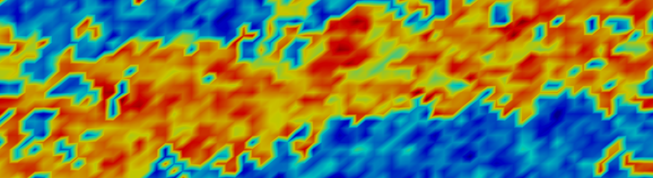
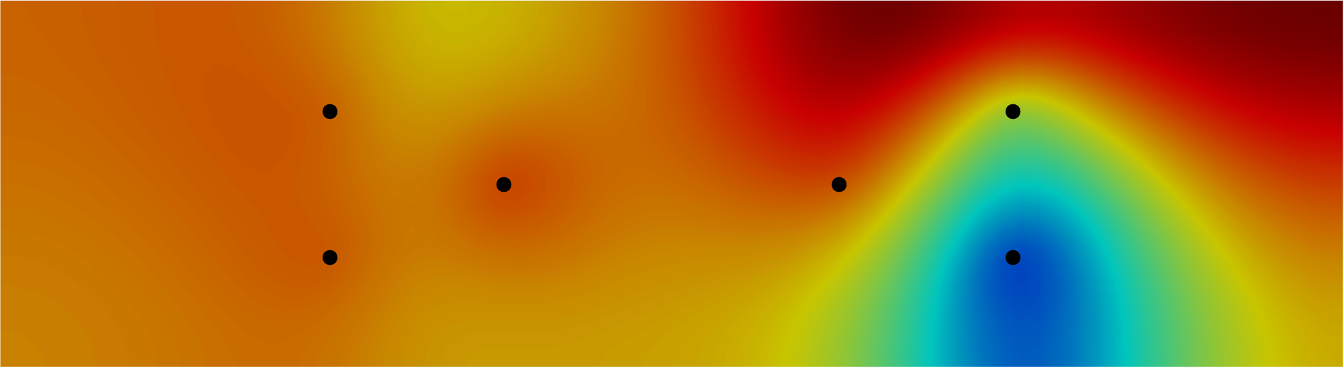
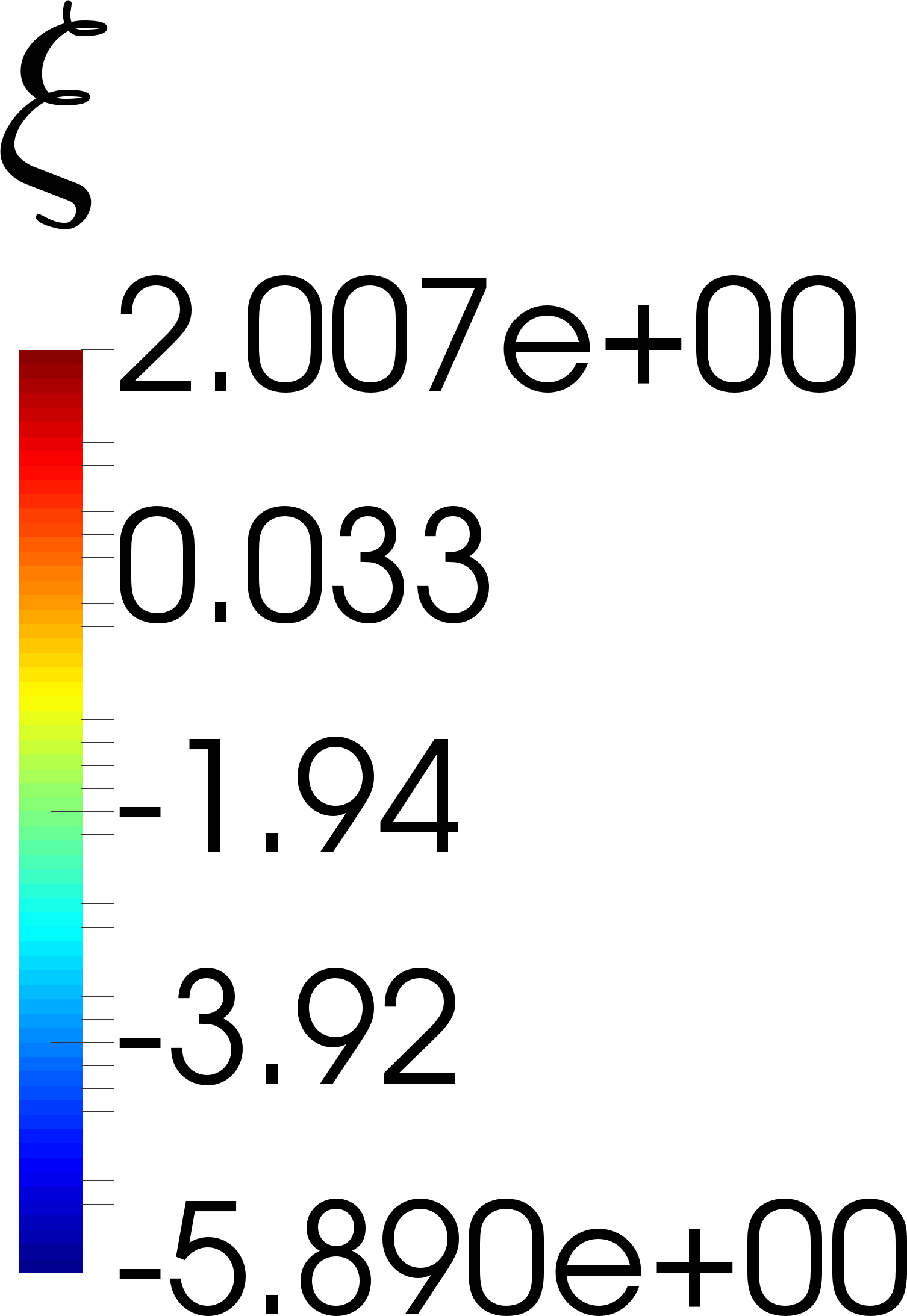
Figure 4: Left: the “true” log permeability field used to generate synthetic pressure data to estimate the log-permeability field. This “true” log-permeability field is a scaled version of the 71st slice of the log-permeability field data from the SPE10 model [1]. Specifically, letting $l(x)$ be the SPE log-permeability data, we use $\theta_{\text{true}}(\mathbf{x})=0.5\left[l(\mathbf{x})-\min(l(\mathbf{x}))\right]+\min(l(\mathbf{x}))$. Right: the maximum a posteriori estimate of the permeability field obtained after solving the Bayesian inverse problem governed by (27) using six pressure observations. The observation locations are shown as black dots.

As synthetic data for estimating $\theta$, we use six noisy pressure observations obtained by solving (27) using a scaled version of the 71st slice of the SPE10 permeability model (shown in Figure 4). We use a bi-Laplacian prior for $\theta$ (see [10]) and assume a Gaussian noise model. The Bayesian inverse problem of estimating $\theta$ using pressure measurements is a nonlinear inverse problem that in general requires a sampling algorithm. We compute an approximate solution to that Bayesian inverse problem using a Laplace approximation to the posterior, which is a Gaussian approximation of the posterior centered at the maximum a posteriori probability (MAP) point; see e.g., [10].

To generate samples of the uncertain velocity field, we proceed as follows: we generate log-permeability field realizations by drawing samples from the approximate posterior for $\theta$; subsequently, we solve the pressure equation to obtain the corresponding pressure fields, which are then used to compute velocity field samples, $\boldsymbol{v}(\theta_{i})$, using Darcy’s Law (26). For illustration, four different Darcy velocity field samples, together with the permeability fields, are shown in Figure 5.

Figure 5: Three log-permeability field samples $\theta_{i}$ and their corresponding velocity fields $\mathbf{v}(\theta_{i})$ (shown as black arrows) obtained from the posterior distribution $\pi_{\theta}$ and the log-permeability field and velocity field corresponding to the MAP point (lower right).

7.2 Uncertainty in the initial time

The second source of irreducible uncertainty we consider is the initial time $T_{0}$. Receiving measurements of the concentration, one usually does not know exactly when the contaminant has been introduced and thus we might only have an estimate for $T_{0}$. This uncertainty of the initial time should be taken into account when computing optimal designs, i.e., optimal designs should be tailored to a range of initial times $T_{0}$. This uncertainty in the initial time is an additional irreducible uncertainty we take into account, and we target designs that are optimized for $T_{0}\in[-1,1]$ and assume $T_{0}\sim\mathcal{U}(-1,1)$.

8 Subsurface flow example: optimal experimental design under uncertainty

In this section we present numerical results for optimal sensor placement under uncertainty and compare results obtained taking into account the irreducible model uncertainty with results that are computed for a fixed realization of the irreducible uncertainty.

8.1 Setup of the OEDUU problem

As explained above, we solve the optimal experimental design under uncertainty (OEDUU) problem using sample average approximation. In our numerical tests, we use 100 Monte Carlo samples of the irreducible model uncertainty $\xi=(\theta,T_{0})$, i.e., $N=100$ in (17). In table 1, we show how many reduced model basis vectors are needed for different tolerances. The moderate growth in the number of needed ROM basis vectors indicates that 100 Monte Carlo samples capture a reasonable amount of the overall uncertainty.

	50	100	300	500
0.002	350	410	469	494
0.0001	881	985	1051	1082

Table 1: Comparison of the number of basis vectors needed to compute $\mathbf{Q}$ and $\widehat{\mathbf{Q}}$ for different numbers $N$ of velocity samples (columns) and tolerances $\mu=0.002$, $0.0001$ (rows). Here, we use Algorithm 2 with one cluster.

As discussed in section 5, minimization of the OEDUU objective (17) is made tractable by elimination of the PDE solves, throughout the optimization iterations, via computation of a composite reduced order basis using algorithm 2. In table 2, we study the accuracy and dimension of the joint basis for different numbers of clusters and choices of $\mu$, which control the accuracy of the reduced models.

Our clustering algorithm sorts the uncertain model parameters into bins based on a distance measure (23) that requires choosing a suitable initial concentration $\mathbf{m}$. Since contaminants in groundwater typically originate from a few localized sources, we choose the initial concentration $\mathbf{m}$, in the definition of the distance measure (23), to be the sum of three radial basis functions with varying centers, spreads and magnitudes. From table 2, we note that for 100 samples of the irreducible uncertainty $\xi$, clustering is not needed as the resulting dimension of $\mathbf{Q}$ and $\widehat{\mathbf{Q}}$ in (21) is rather small. For smaller choices of $\mu$, such as $\mu=10^{-4}$, or larger numbers of samples, clusters becomes more important to reduce memory usage and compute time.

We find that the joint basis obtained using 1 cluster and $\mu=0.002$ is sufficient for our purposes, both for approximation of the OEDUU objective $\phi_{\text{N}}$ in (17) and approximation of $\widetilde{\mathbf{F}}_{i}$ for each forward operator sample. Thus, this choice of parameters is used henceforth.

	$\boldsymbol{\mu}$	Number basis vectors	Error
1 Cluster	$0.002$	410	$6.876\times 10^{-4}$
	$0.0001$	985	$2.335\times 10^{-6}$
4 Clusters	$0.002$	283,267,271,279	$8.348\times 10^{-4}$
	$0.0001$	667,751,710,731	$7.943\times 10^{-6}$

Table 2: Comparison of ROMs obtained using algorithm 2 with $\mu=0.002$, $0.0001$ and different numbers of clusters. Using $N=100$ sample velocity fields and initial times, $\phi_{N}(\mathbf{w})$ in objective (17) is computed for $\mathbf{w}=[1,\ldots,1]$, i.e., the design which includes all sensor locations. The relative error in column four is computed as $\frac{|{\phi_{N}}(\mathbf{w})-{\phi^{t}_{N}}(\mathbf{w})|}{|{\phi^{t}_{N}}(\mathbf{w})|}$, where the true value ${\phi^{t}_{N}}(\mathbf{w})$ was approximated using a reduced basis computed using algorithm 2 with $\mu=10^{-6}$. The third column shows how many basis vectors $k$ were needed in the algorithm to obtain the desired accuracy as described by line 6 in algorithm 2.

To obtain sparse and binary optimal designs, we solve a sequence of minimization problems of the form (17). Following the sparsification approach outlined in section 3.3, we use penalty functions of the form (8) with $\alpha=0.1$ and $\varepsilon(i)=\left(\frac{2}{3}\right)^{i}$, $i=1,2,3,\ldots$. For our problem setup, the weights converge to binary values in approximately 20 iterations of the sparsification procedure. In our computations, we use the Broyden-Fletcher-Goldfarb-Shannon (BFGS) method available in python’s scipy library. We supply this minimization algorithm with the objective function and its gradient as described in section 4.

8.2 Solving the OEDUU problem

Here, we demonstrate that solving the OEDUU problem with our proposed approach is effective in producing designs for which the expected value of the posterior uncertainty (5) is small. In particular, we numerically verify that the SAA (11) is a reasonable approximation. This is done by solving the OEDUU problem with $N=100$ SAA samples, and comparing the expected value of the objective obtained using the optimal experimental designs under uncertainty, which we will refer to as uncertainty-aware designs, with that obtained with deterministic designs. By deterministic designs we mean optimal designs obtained using a single sample from the irreducible uncertainty (velocity field and initial time); this amounts to minimizing (17) with $N=1$.

The results are shown in Figure 6. To obtain designs with different numbers of sensors, (17) was solved for different regularization parameters $\gamma$, which indirectly controls the sparsity of the optimal designs. To approximate the expectation shown on the $y$-axis, we use a Monte Carlo approximation of the expectation of the trace update $\mathbb{E}\left[\tr\left(\mathbf{K}(\xi,\mathbf{w})\right)\right]$ with 100 samples from the irreducible uncertainty that are drawn independently from the SAA samples used to compute the uncertainty-aware designs. Additionally, to avoid bias due to the model reduction, we use more accurate reduced models, specifically we use Algorithm 2 with $\mu=10^{-4}$.

If the sampling as well as the model reduction errors are small enough, we would expect that the uncertainty-aware designs reduce the expected trace more than deterministic designs. As can be seen in Figure 6, this is the case most of the time, i.e., we find good binary minimizers of the objective (5). Only very few deterministic designs are superior to the uncertainty-aware designs, which is likely due to sampling error.

Figure 6: Trace reduction ${\phi_{N}}$ in objective (16) for deterministic OED (light blue dots) and OEDUU (red diamonds). The irreducible uncertainty for the uncertainty-aware designs is approximated using 100 samples from the irreducible uncertainty (velocity field and initial times). The deterministic designs are computed for 20 samples from the irreducible uncertainty. The $x$-axis shows the number of sensors for each design. The expectation in the objective, which is shown on the $y$-axis, is approximated using 100 samples that are chosen independently from the samples used to compute the designs.

8.3 Quality of the computed optimal designs

Ultimately, our goal is to choose the sensors for data collection which will allow us to learn the most about the initial concentration for a fixed velocity field and initial time $T_{0}$. Here we demonstrate numerically that the designs computed via OEDUU perform better (produce more informative data) on average than deterministic designs computed for realizations of the irreducible model uncertainty.

Here, we study the effectiveness of the same uncertainty-aware designs used above not in expectation, but for 100 individual realizations $\xi_{i}$ of the irreducible uncertainty, which again differ from the SAA samples used to compute the uncertainty-aware designs. Results are shown in Figure 7, where now we show percentiles for the trace updates for individual $\xi_{i}$.

We observe that the designs obtained using OEDUU tend to have a smaller mean in the update trace than the designs obtained using individual $\xi_{i}$, particularly when we only use few sensors. Additionally, the 25th–75th and 2nd–98th percentiles show that poorly performing designs are less likely when one accounts for the uncertainty in the design computation. This is again, particularly the case for designs with small numbers of sensors. We believe that the reason for diminishing benefit of computing designs under uncertainty for larger number of sensors is that at each sensor location, 5 measurements in time are used. Thus, most information about the initial condition that can be recovered is already available from a rather small number of sensors and thus different designs play a less important role. Here, the diffusion contained in the governing PDE plays an important role as well, as it limits the resolution of the initial condition reconstruction that can be obtained from observations. This is also reflected by the decreasing gain of using more than 5 sensors.

The benefit of computing uncertainty-aware designs is greater for inverse problems where less information can be gained at each sensor location. This can be seen in Figure 8. To obtain these results, we use the same inverse problem and ROM setup as described in Sections 6-8.1 but restrict the times at which we can measure data to $\tau_{i}=12,15$, effectively reducing the amount of information gathered at sensors and increasing the importance of careful sensor placement. Comparing Figures 7 and 8, we can see that for “harder” inverse problems, i.e., those with less-informative data, the difference between uncertainty-aware designs and deterministic designs is more significant.

Figure 7: Comparing the mean for the trace in the deterministic objective, $\phi_{N}$ with $N=1$ in (16), using deterministic designs and designs taking into account the uncertainty. The uncertainty-aware designs and the deterministic designs are the same as used in Figure 6. Each design is used to evaluate the deterministic objective for 100 realizations of the irreducible uncertainty. The sample mean is plotted as a solid line and the shaded regions depict the 25th–75th and 2nd–98th percentile envelopes (for both the mean and the envelopes, red is used for uncertainty-aware designs and blue for deterministic designs).

Figure 8: Same as Figure 7, but with only two time observations at $\tau_{i}=12,15$ (rather than five). In this regime with less observations, the uncertainty-aware design outperforms deterministic designs more significantly also for larger numbers of sensors.

9 Discussion and conclusions

We have developed a mathematical formulation and numerical scheme for computing A-optimal experimental designs for infinite-dimensional Bayesian linear inverse problems governed by PDEs with irreducible model uncertainty. The proposed measurement space approach replaces trace estimation in an infinite-dimensional (high-dimensional upon discretization space) with trace estimation in the (finite-dimensional) measurement space. The computation of a joint reduced basis capturing the action of the forward operators for different random samples allows efficient computation of optimal designs. Numerical experiments for the inversion of initial concentration of a contaminant in groundwater indicate that, on average, designs that take the model uncertainty into account are superior to those that do not. This superiority is less pronounced as more sensors are being used.

We have used a Monte Carlo approach for dealing with uncertainty, which can require many samples for adequate resolution. A possible extension of our work is to consider alternate approaches for approximating the uncertainty, e.g., Taylor expansions of the uncertainty or stochastic approximation (SA). In the latter, the samples for the irreducible uncertainty are not chosen a priori, but are varied during the optimization. This avoids potential bias of the design towards the chosen samples but leads to several additional challenges in the optimization. Another important research question is the generalization of our approach to nonlinear inverse problems. One possibility is to follow the framework in [4], which is based on Gaussian approximations at the MAP point. Clearly, nonlinear problems under uncertainty become computationally rather expensive.

One aspect of OED under model uncertainty that is not explored in the present work is that of dealing with reducible sources of model uncertainty, i.e., additional uncertainties that could be reduced through observational data. However, the focus might be on estimation of primary parameters of interest and not on estimation of this (secondary) reducible uncertainty. Hence, the design should be chosen to focus mainly on the primary parameter and only on the secondary parameters to the extent that it aids inference of the primary parameters.

References

- [1] SPE comparative solution project. https://www.spe.org/web/csp/datasets/set02.htm.
- [2] Alen Alexanderian, Philip J Gloor, Omar Ghattas, et al. On Bayesian A-and D-optimal experimental designs in infinite dimensions. Bayesian Analysis, 11(3):671–695, 2016.
- [3] Alen Alexanderian, Noemi Petra, Georg Stadler, and Omar Ghattas. A-optimal design of experiments for infinite-dimensional Bayesian linear inverse problems with regularized -sparsification. SIAM Journal on Scientific Computing, 36(5):A2122–A2148, 2014.
- [4] Alen Alexanderian, Noemi Petra, Georg Stadler, and Omar Ghattas. A fast and scalable method for A-optimal design of experiments for infinite-dimensional Bayesian nonlinear inverse problems. SIAM Journal on Scientific Computing, 38(1):A243–A272, 2016.
- [5] Alen Alexanderian and Arvind K. Saibaba. Efficient D-optimal design of experiments for infinite-dimensional Bayesian linear inverse problems. SIAM Journal on Scientific Computing, 40(5):A2956–A2985, 2018.
- [6] Anthony C. Atkinson and Alexander N. Donev. Optimum Experimental Designs. Oxford, 1992.
- [7] Ahmed Attia, Alen Alexanderian, and Arvind K Saibaba. Goal-oriented optimal design of experiments for large-scale bayesian linear inverse problems. Inverse Problems, 34(9):095009, 2018.
- [8] Jacob Bear. Modeling phenomena of flow and transport in porous media, volume 31. Springer, 2018.
- [9] Hans-Georg Beyer and Bernhard Sendhoff. Robust optimization—a comprehensive survey. Computer Methods in Applied Mechanics and Engineering, 196(33):3190–3218, 2007.
- [10] Tan Bui-Thanh, Omar Ghattas, James Martin, and Georg Stadler. A computational framework for infinite-dimensional Bayesian inverse problems Part I: The linearized case, with application to global seismic inversion. SIAM Journal on Scientific Computing, 35(6):A2494–A2523, 2013.
- [11] Emmanuel J Candes, Michael B Wakin, and Stephen P Boyd. Enhancing sparsity by reweighted minimization. Journal of Fourier analysis and applications, 14(5-6):877–905, 2008.
- [12] Yair Daon and Georg Stadler. Mitigating the influence of the boundary on PDE-based covariance operators. Inverse Problems & Imaging, 12(5):1083–1102, 2018.
- [13] Masoumeh Dashti and Andrew M. Stuart. The Bayesian Approach to Inverse Problems, pages 311–428. Springer International Publishing, 2017.
- [14] Gene H Golub and Charles F Van Loan. Matrix computations, volume 3. JHU press, 2012.
- [15] Eldad Haber, Lior Horesh, and Luis Tenorio. Numerical methods for experimental design of large-scale linear ill-posed inverse problems. Inverse Problems, 24(055012):125–137, 2008.
- [16] Eldad Haber, Lior Horesh, and Luis Tenorio. Numerical methods for the design of large-scale nonlinear discrete ill-posed inverse problems. Inverse Problems, 26(2):025002, 2010.
- [17] Eldad Haber, Zhuojun Magnant, Christian Lucero, and Luis Tenorio. Numerical methods for A-optimal designs with a sparsity constraint for ill-posed inverse problems. Computational Optimization and Applications, pages 1–22, 2012.
- [18] Nathan Halko, Per Gunnar Martinsson, and Joel A. Tropp. Finding structure with randomness: Probabilistic algorithms for constructing approximate matrix decompositions. SIAM Review, 53(2):217–288, 2011.
- [19] Lior Horesh, Eldad Haber, and Luis Tenorio. Optimal Experimental Design for the Large-Scale Nonlinear Ill-Posed Problem of Impedance Imaging, pages 273–290. Wiley, 2010.
- [20] Xun Huan and Youssef M. Marzouk. Simulation-based optimal Bayesian experimental design for nonlinear systems. Journal of Computational Physics, 232(1):288–317, 2013.
- [21] Stefan Körkel, Ekaterina Kostina, Hans G. Bock, and Johannes P. Schlöder. Numerical methods for optimal control problems in design of robust optimal experiments for nonlinear dynamic processes. Optimization Methods & Software, 19(3-4):327–338, 2004. The First International Conference on Optimization Methods and Software. Part II.
- [22] Drew P Kouri and Alexander Shapiro. Optimization of PDEs with uncertain inputs. In Frontiers in PDE-Constrained Optimization, pages 41–81. Springer, 2018.
- [23] Quan Long, Marco Scavino, Raúl Tempone, and Suojin Wang. Fast estimation of expected information gains for Bayesian experimental designs based on Laplace approximations. Computer Methods in Applied Mechanics and Engineering, 259:24–39, 2013.
- [24] Ira Neitzel, Konstantin Pieper, Boris Vexler, and Daniel Walter. A sparse control approach to optimal sensor placement in PDE-constrained parameter estimation problems. arXiv preprint arXiv:1905.01696, 2019.
- [25] Andrej Pázman. Foundations of Optimum Experimental Design. D. Reidel Publishing Co., 1986.
- [26] Benjamin Peherstorfer, Daniel Butnaru, Karen Willcox, and Hans-Joachim Bungartz. Localized discrete empirical interpolation method. SIAM Journal on Scientific Computing, 36(1):A168–A192, 2014.
- [27] Friedrich Pukelsheim. Optimal Design of Experiments. John Wiley & Sons, New-York, 1993.
- [28] Lassi Roininen, Janne MJ Huttunen, and Sari Lasanen. Whittle-Matérn priors for Bayesian statistical inversion with applications in electrical impedance tomography. Inverse Probl. Imaging, 8(2):561, 2014.
- [29] Lars Ruthotto, Julianne Chung, and Matthias Chung. Optimal experimental design for inverse problems with state constraints. SIAM Journal on Scientific Computing, 40(4):B1080–B1100, 2018.
- [30] Nikolaos V Sahinidis. Optimization under uncertainty: state-of-the-art and opportunities. Computers & Chemical Engineering, 28(6):971–983, 2004.
- [31] Alexander Shapiro, Darinka Dentcheva, and Andrezj Ruszczynski. Lectures on Stochastic Programming: Modeling and Theory. Society for Industrial and Applied Mathematics, 2009.
- [32] Dariusz Uciński. Optimal measurement methods for distributed parameter system identification. CRC Press, Boca Raton, 2005.
- [33] Umberto Villa, Noemi Petra, and Omar Ghattas. hIPPYlib: An Extensible Software Framework for Large-Scale Inverse Problems Governed by PDEs; Part I: Deterministic Inversion and Linearized Bayesian Inference. arXiv preprint arXiv:1909.03948, 2019.
- [34] Jing Yu and Mihai Anitescu. Multidimensional sum-up rounding for integer programming in optimal experimental design. Mathematical Programming, pages 1–40, 2017.