NT@UW-19-20
The Frame-Independent Spatial Coordinate ${\tilde{z}}$: Implications for Light-Front Wave Functions, Deep Inelastic Scattering, Light-Front Holography, and Lattice QCD Calculations

Abstract

A general procedure for obtaining frame-independent, three-dimensional light-front coordinate-space wave functions is introduced. The third spatial coordinate, ${\tilde{z}}$ , is the frame independent coordinate conjugate to the light-front momentum coordinate $x={k^{+}\over P^{+}}$ which appears in the momentum-space light-front wave functions underlying generalized parton distributions, structure functions, distribution amplitudes, form factors, and other hadronic observables. These causal light-front coordinate-space wave functions are used to derive a general expression for the quark distribution function of hadrons as an integral over the frame-independent longitudinal distance (the Ioffe time) between virtual-photon absorption and emission appearing in the forward virtual photon-hadron Compton scattering amplitude. Specific examples using models derived from light-front holographic QCD show that the spatial extent of the proton eigenfunction in the longitudinal direction can have very large extent in ${\tilde{z}}$.

Introduction

Much recent effort has been devoted to understanding and measuring the generalized parton distributions Mueller:1998fv ; Ji:1996ek ; Radyushkin:1996nd which encode the fundamental structure of hadrons in terms of the three-dimensional momentum-space coordinates of their quark and gluon constituents. Recent lattice calculations of quasi-pdfs evaluate a Fourier transform of a matrix element which depends on the spatial separation between the points of virtual-photon absorption and emission that appears in the virtual photon-proton Compton scattering amplitude. It is therefore of considerable interest to understand the spatial longitudinal dependence of the virtual Compton amplitude from a causal, frame-independent perspective. In this paper we show that the frame-independent eigensolutions of the QCD light-front Hamiltonian that underly hadronic observables can be expressed in terms of a longitudinal spatial coordinate ${\tilde{z}}$ that is simply related to the spatial separation between a struck quark and the spectators. One thus obtains a frame-independent fully three-dimensional spatial description of hadron structure which complements analyses using the usual transverse spatial variables Soper:1976jc ; Burkardt:2002hr ; Miller:2007uy ; Miller:2010nz .

The Light-Front Fock Representation

The light-front expansion of any hadronic system is constructed by quantizing quantum chromodynamics at fixed light-front time $\tau=t+z/c$ Dirac:1949cp ; Brodsky:1973kr ; Brodsky:1979qm ; Brodsky:1997de ; Brodsky:2000ii . The LF time-evolution operator $P^{-}=i\frac{d}{d\tau}$ can be derived directly from the QCD Lagrangian. The light-front Lorentz-invariant Hamiltonian for the composite hadrons $H_{LF}^{QCD}=P^{-}P^{+}-{\bf P}^{2}$ ($P^{\pm}=P^{0}\pm P^{z}$ and boldface denotes the two-dimensional transverse vectors) has eigenvalues ${\cal M}^{2}_{h}$, corresponding to the mass spectrum of the color-singlet states in QCD Brodsky:1997de .

In principle, the complete set of bound-state and scattering eigensolutions of $H_{LF}^{QCD}$ can be obtained by solving the light-front Heisenberg equation $H_{LF}^{QCD}\,\left|\,{\psi_{h}}\right\rangle={\cal M}^{2}_{h}\,\left|\,{\psi_{h}}\right\rangle,$where $\,\left|\,{\psi_{h}}\right\rangle$ is an expansion in multi-particle Fock eigenstates $\{\,\left|\,{n}\right\rangle\}$ of the free light-front Hamiltonian: $|\psi_{h}\rangle=\sum_{n}\psi_{n/h}|\psi_{h}\rangle.$ The light-front wavefunctions $\psi_{n/h}(x_{i},{\bf k}_{i},\lambda_{i})$ provide a complete, causal, frame independent representation of a hadrons, relating the quark and gluon degrees of freedom in each $n$-particle Fock state to the hadronic eigenstate.

Twist-two operators and the need for a longitudinal spatial coordinate 

The quark distributions of a hadron are matrix elements of quark operators at light-like separation Collins:1981uw ; Ji:1998pc ; Collins:2003fm ; Tanabashi:2018oca :

$$q(x)=\int{dx^{-}\over 4\pi}e^{ixP^{+}x^{-}}\langle P|\overline{\psi}(-{x^{-}\over 2})\gamma^{+}\psi({x^{-}\over 2})|P\rangle,$$

$$\overline{q}(x)=-q(-x),$$ (1)

where the notation $(x^{-}/2)$ refers to the four vector $(x^{-}/2,x^{+}=0,{\bf x}=0)$; the LF helicity and flavor labels, as well as the $Q^{2}$-dependence, are suppressed. The operator $\gamma^{0}\gamma^{+}$ that appears in the matrix element in $A^{+}=0$ gauge serves to project Brodsky:1973kr the dependent field operator $\psi$ onto its independent component $\psi_{+}$, so that field operators and their adjoints appear. The variable $x$ ranges between $0$ and $1$.

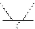
Figure 1: Forward virtual Compton scattering.

The expression for $q(x)$ is the leading-twist approximation to the virtual photon forward scattering amplitude shown in Fig. 1, and $x^{-}$ is the distance along the light cone between the emission and absorption of the virtual photon. The complete interpretation of the spatial dependence of the quark distributions requires an understanding of their contributions to $q(x)$ as a function of the longitudinal spatial separation $x^{-}$.

The matrix element appearing in Eq. (1) is directly relevant to several techniques that seek to obtain quark distributions as functions of $x$, e. g. Refs.Ji:2013dva ; Lin:2018qky ; Alexandrou:2018pbm ; Sufian:2019bol . See the extensive reviews Cichy:2018mum ; Monahan:2018euv . These techniques represent significant advances over efforts based on computing moments of distributions. Lattice theorists compute the lattice version of the matrix element appearing in Eq. (1), for example, Alexandrou:2018pbm , as $h_{\gamma^{+}}(P,x^{-}),$ and then take a Fourier transform in order to obtain the quasi-pdfs. Therefore it is useful to obtain physical intuition regarding the matrix element appearing in Eq. (1). This will be done here by employing recent models derived from holographic light- front QCD.

Of course we are not the first to study the variable $x^{-}$. It has commonly been called the Ioffe time Gribov:1965hf ; Ioffe:1969kf ; Kovchegov:2012mbw . This quantity is known to be large if $x$ is small. The study of the matrix element appearing in Eq. (1) as the Fourier transform of quark probability distributions was initiated in Ref. Braun:1994jq ; Braun:2007wv . Our procedure elucidates the dependence on $x^{-}$ that appears in Eq. (1) as derived from light-front wave functions in coordinate space, and it is thus not the same as the procedure of Ref. Braun:1994jq ; Braun:2007wv .

We study hadronic light-front wave functions as a function of the longitudinal spatial coordinate of the quark and gluon constituents. The appearance of wave functions arises by inserting a complete set of states $|n-1\rangle$ in Eq. (1) so that

$$q(x)=2^{1/2}\int{dx^{-}\over 4\pi}e^{ixP^{+}x^{-}}\times$$

$$\sum_{n}\langle P|\psi_{+}^{\dagger}(-{x^{-}\over 2})|n-1\rangle\langle n-1|\psi_{+}({x^{-}\over 2})|P\rangle.$$ (2)

The quantity $\langle n-1|\psi({x^{-}\over 2})|P\rangle$ is an overlap of amplitudes which projects out the active, struck quark, integrated over the spectator particles. This is simply the light front Fock space wave function of a quark (or anti-quark). In the momentum space representation of the standard Fock space description Brodsky:1979qm ; Brodsky:1997de ; Brodsky:2000ii , one has for the quark distributions $\langle n-1|\psi_{+}{({x},{\bf k},\lambda})|P\rangle\equiv\psi_{n}(x,{\bf k},\lambda)2^{-1/4},$ in which the indices that refer to specific states have been suppressed to simplify the presentation. The contribution of this component ($q_{n}$) $q(x)$ of Eq. (1) is given by

$$q_{n}(x)=\int{d^{2}k\over(2\pi)^{2}}\left|\psi_{n}(x,{\bf k})\right|^{2},$$ (3)

For quarks $\left|\psi_{n}(x,{\bf k},\lambda))\right|^{2}\propto|\langle n-1|b(k^{+},{\bf k},\lambda)|P\rangle|^{2}$, where $b(k^{+},{\bf k},\lambda)$ is the destruction operator and for anti-quarks $\left|\psi_{n}(x,{\bf k},\lambda))\right|^{2}\propto|\langle n-1|d(k^{+},{\bf k},\lambda)|P\rangle|^{2}$, Jaffe:1983hp ; Diehl:2003ny .

Converting these momentum-space wave functions to coordinate space is the next step. The transverse momentum coordinate ${\bf k}$ is transformed into the canonically conjugate impact parameter ${\bf b}$ to obtain $\psi_{n}({x},{\bf b})$ using standard methods Soper:1976jc ; Burkardt:2002hr ; Miller:2007uy ; Miller:2010nz . The dependence of $\psi_{n}$ on the frame-independent longitudinal spatial coordinate has not previously appeared.

The frame-independent longitudinal space coordinate ${\tilde{z}}$

The momentum space wave functions are normally expressed in terms of the longitudinal light-front momentum coordinate $k_{i}^{+}\over P^{+}$, where the index $i$ refers to the $i$’th constituent. The canonical spatial coordinate is therefore given by the frame-independent variable

$${\tilde{z}}_{i}=P^{+}x^{-}_{i}.$$ (4)

Our ${\tilde{z}}_{i}$ seems similar to the variable $z$ of  Braun:1994jq , but its origin and meaning is different. The canonical spatial coordinate occurs for each of the constituents of a Fock space component of a hadronic wave function. When dealing with the light front wave functions defined above, all of the constituents save one are integrated out. Therefore in the following we use ${\tilde{z}}$ instead of ${\tilde{z}}_{i}$ to simplify the notation. See also Radyushkin:2017cyf ; Orginos:2017kos .

Making a standard Fourier transform yields the coordinate space wave function given by

$$\psi_{n}({\tilde{z}},{\bf b})={1\over\sqrt{2\pi}}\int_{0}^{1}dx\,\psi_{n}(x,{\bf b})e^{i{\tilde{z}}x},$$ (5)

or the mixed form

$$\psi_{n}({\tilde{z}},{\bf k})={1\over\sqrt{2\pi}}\int_{0}^{1}dx\,\psi_{n}(x,{\bf k})e^{i{\tilde{z}}x}.$$ (6)

These light-front (LF) wave functions are independent of the observer’s Lorentz frame since both the longitudinal and transverse coordinates are canonically conjugate to relative LF momentum coordinates.

It is worthwhile to compare the present approach with the concept that the longitudinal direction is Lorentz-contracted to zero in the infinite momentum frame. Contraction occurs if one identifies the longitudinal coordinate as $x^{-}$, the coordinate canonically conjugate to the momentum variable $k^{+}$. This leads to a frame-dependent coordinate-space wave function from the relation:

$$\chi_{P}^{+}(x^{-},b)=\sqrt{P^{+}\over{2\pi}}\int_{0}^{1}dx\psi_{n}(x,{\bf b})e^{ix^{-}P^{+}x}$$ (7)

The resulting density $\rho_{P^{+}}(x^{-},b)=|\chi_{P^{+}}(x^{-},b)|^{2},$ in the infinite momentum frame is obtained by taking $P^{+}$ to $\infty$. Taking the limit carefully Dumitru:2018vpr yields $\rho(x^{-},b)=\int{dx}|\psi_{n}(x,b)|^{2}\delta(x^{-}),$ a result that corresponds to a picture in which GPDs are represented as disks Accardi:2012qut . See also Ref. Hoyer:2006xg . There is one caveat: the contraction occurs only for matrix elements of the independent quark-field operators involving the so-called “good” operator $\gamma^{+}$.

However, there is an obvious problem associated with using the frame-dependent $x^{-}$ coordinate in the infinite momentum frame. The Lorentz invariant distribution is obtained using instead the boost invariant longitudinal coordinate ${\tilde{z}}=P^{+}x^{-}$.

The variable $x^{-}$ from light-front wave functions

The frame-independent quark distribution function $q_{n}(x)$ of Eq. (3) can be expressed in terms of the longitudinal coordinate ${\tilde{z}}$ using the inverse Fourier transform of Eq. (6) so that

$$q_{n}(x)=\int{d{\tilde{z}}d{\tilde{z}}^{\prime}\over 2\pi}\int{d^{2}{\bf k}\over(2\pi)^{2}}\psi_{n}^{*}({\tilde{z}}^{\prime},{\bf k})\psi_{n}({\tilde{z}},{\bf k})e^{i({\tilde{z}}-{\tilde{z}}^{\prime})x}$$

(8)

Letting $R\equiv({\tilde{z}}+{\tilde{z}}^{\prime})/2$, $x^{-}={\tilde{z}}-{\tilde{z}}^{\prime}$ and integrating over $R$ yields

$$q_{n}(x)=\int^{\infty}_{-\infty}dx^{-}g_{n}(x^{-},x),$$ (9)

with

$$g_{n}(x^{-},x)={1\over 2\pi}\int_{0}^{1}dy\,q_{n}(y)\cos{x^{-}(y-x)}.$$ (10)

The function $g_{n}(x^{-},x)$ is a measure of the contribution to quark (anti-quark) distribution functions that occur at a particular value of $x^{-}$. In contrast with the distributions of  Braun:1994jq , this quantity is real-valued because it is derived from the real-valued quantity of Eq. (8).

Models to further our understanding of $g(x^{-},x)$

The first model considered is that of a pseudoscalar meson with massless quarks and one valence $q\overline{q}$ Fock space component. This is the LF holographic model for the massless pion in the chiral $m_{q}=0$ limit. The eigenfunction of the holographic light front Hamiltonian Brodsky:2007hb is given by:

$$\psi_{M}(x,{\bf b})={\kappa\over\sqrt{\pi}}\sqrt{x(1-x)}e^{-{{\bf b}^{2}\kappa^{2}x(1-x)\over 2}}.$$ (11)

The transverse variable Brodsky:2007hb $\zeta^{2}=b^{2}x(1-x)$ is canonically conjugate to $k^{2}\over x(1-x)$ and the wave functions are simplified if this variable is used. Here we take another path by exhibiting the separate dependence of $x^{-}$ and transverse coordinates.

The momentum space version of Eq. (11), relevant for evaluating $g(x^{-},x)$, is obtained from the Fourier transform to the canonically conjugate ${\bf k}$ so that

$$\psi_{M}(x,{\bf k})={2\sqrt{\pi}\over\kappa\sqrt{x(1-x)}}e^{-{{\bf k}^{2}\over 2\kappa^{2}x(1-x)}}.$$ (12)

Using Eq. (3) one finds that the parton distribution is constant for this model, obtained with massless quarks, $q^{M}(x)={1}.$ In contrast, for $m_{q}\neq 0$ one  Brodsky:2014yha models the mass-dependence so that $q^{M}(x)=\exp(-{m^{2}_{q}\over\kappa^{2}x(1-x)})$.

The coordinate space wave function is obtained by using Eq. (5). It is useful to define a light-front coordinate-pace density:

$$\rho_{M}({\tilde{z}},b)\equiv|\psi_{M}^{S}({\tilde{z}},b)|^{2}.$$ (13)

This gives the probability that the struck constituent is separated from the spectators by a longitudinal distance ${\tilde{z}}$ and a transverse separation $b$. Thus obtaining $\rho_{M}({\tilde{z}},b)$ provides a new way of examining hadronic wave functions.

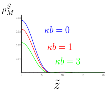
Figure 2: The density $\rho^{S}_{M}({\tilde{z}},b)$ values of $\kappa b=0,1,3$

This is shown for $m_{q}=0$ in Fig. 2. An interesting feature is that for each value of $\kappa b$ the density vanishes at values of ${\tilde{z}}\approx 7.6$.

We may gain an understanding of this behavior by obtaining a closed form expression for $\psi_{M}^{S}({\tilde{z}},b)$. By changing variables to $u=x-1/2$ and expanding the exponential in powers of $\lambda\equiv\kappa^{2}b^{2}/8$ we find the most important term to be

$${\sqrt{2\pi}\over 2\kappa}\ \psi_{M}^{S}({\tilde{z}},b)\approx{\pi\over 4}e^{i{\tilde{z}}/2}\,e^{-b^{2}\kappa^{2}/8}{J_{1}({\tilde{z}}/2)\over{\tilde{z}}},$$ (14)

which is reasonably accurate for ${\tilde{z}}$ greater than about $b^{2}\kappa^{2}$. The first zero of $J_{1}(x)$ occurs at $x=3.8171$; one can obtain a qualitative understanding of this zero crossing as shown in Fig. 2. The result Eq. (14) means that for such values, the density falls only as $1/{\tilde{z}}^{3}$ approximately modulated by $\cos^{2}({{\tilde{z}}+\pi/4})$. The existence of such a large-distance tail indicates that using the ${\tilde{z}}$ variable has the potential to reveal interesting aspects of hadronic physics.

The next step is to determine the function $g(x^{-},x)$ for the model of Eq. (11). Use Eq. (10) with $q_{n}(y)=1$ as given above, so that

$$g_{M}(x^{-},x)={1\over 2\pi}\frac{\sin(x^{-}x)+\sin(x^{-}(1-x))}{x^{-}}.$$ (15)

Observe the slow, $1/x^{-}$, falloff with increasing values of $x^{-}$ for all values of $x$.

Similarly, a slow falloff is also obtained for models with massive quarks. In the limit of large quark masses, defined by $\gamma\equiv m_{q}^{2}/\kappa^{2}>1$, we find that

$$g_{M}(x^{-},x)\approx\frac{e^{-4\gamma}e^{-\frac{{(x^{-})}^{2}}{64\gamma}}\cos\left(x^{-}\left(x-\frac{1}{2}\right)\right)}{8\sqrt{\pi}\sqrt{\gamma}}.$$ (16)

Universal Light Front Wave Functions deTeramond:2018ecg

The model given in Eq. (11) is very simple, with $q_{n}(x)=1$ for $m_{q}=0.$ A recent paper deTeramond:2018ecg presents a universal description of generalized parton distributions obtained from Light-Front Holographic QCD, and we shall use their models for light-front wave functions. These are presented as functions of the number $\tau$ of constituents of a Fock space component. Regge behavior at small $x$ and inclusive counting rules as $x\rightarrow 1$ are incorporated. Nucleon and pion valence quark distribution functions are obtained in precise agreement with global fits. The model is described by the quark distribution $q_{\tau}(x)$ and the profile function $f(x)$ with

$$q_{\tau}(x)=\frac{1}{N_{\tau}}\big{(}1-w(x)\big{)}^{\tau-2}\,w(x)^{-{\frac{1}{2}}}\,w^{\prime}(x),$$ (17)

$$f(x)=\frac{1}{4\lambda}\left[(1-x)\log\left(\frac{1}{x}\right)+a(1-x)^{2}\right],$$ (18)

and $w(x)=x^{1-x}e^{-a(1-x)^{2}}.$

The value of the universal scale $\lambda$ is fixed from the $\rho$ mass: $\sqrt{\lambda}=\kappa=m_{\rho}/\sqrt{2}=0.548$ GeV Brodsky:2014yha ; Brodsky:2016yod . The flavor-independent parameter $a=0.531\pm 0.037$. The $u$ and $d$ quark distributions of the proton are given by a linear superposition of $q_{3}$ and $q_{4}$ while those of the pion are obtained  deTeramond:2010ez from $q_{2}$ and $q_{4}$.

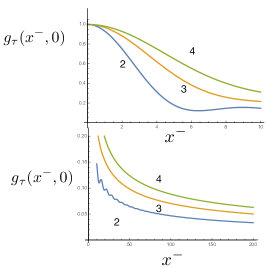
Figure 3: $g_{\tau}(x^{-},0)$. The numbers refer to the value of $\tau$, the number of constituents in the Fock state.

Given these distributions we may study the function $g(x^{-},x)$ of as a function of $\tau$, using Eq. (10) with $q_{\tau}$ replacing $q_{n}$. Fig. 3 shows $g(x^{-},0)$ as a function of $x^{-}$, the dimensionless separation between the emission and absorption of the photon $x^{-}$ of Fig. 1. In the lab frame $x^{-}=\sqrt{2}/Mx^{-}=0.3x^{-}$ fm, so that the proton radius corresponds to about $x^{-}=3.$ One observes a slow falloff with increasing $x^{-}$: $g_{\tau}(x^{-})\sim{1\over\sqrt{x^{-}}}$ for all values of $\tau$. This qualitative behavior can be understood analytically. The function $q_{\tau}(x)\sim 1/\sqrt{x}$ for small values of $x$ and $(1-x)^{2\tau-3}$. A useful approximation for $q_{\tau}(x)$ is given by the product of the two forms. In that case one may consider e.g.

$$\int_{0}^{1}{dy\over\sqrt{y}}\,(1-y)^{3}\cos{x^{-}(y-x)}$$ (19)

$$\sim\frac{\sqrt{2\pi}{(x^{-})}^{3/2}\sin(x)+\sqrt{2\pi}{(x^{-})}^{3/2}\cos(x)+3\cos(x-{x^{-}})}{2{(x^{-})}^{2}}$$ (20)

which, for all values of $x$, demonstrates $(x^{-})^{-1/2}$ falloff, modulated by oscillatory behavior. An essential feature is that there is a significant probability that the deep inelastic scattering process occurs at large separations between the absorption and emission of the virtual photon.

The traditional idea that large longitudinal distances (the Ioffe time) Ioffe:1969kf ; Braun:1994jq , underlies deep inelastic scattering at small $x_{bj}$ is related to the hadronic light-front wave function.

Ref. deTeramond:2018ecg also presents the universal light front wave function (LFWF):

$$\psi_{\rm eff}^{\tau}(x,\mathbf{b})=\frac{1}{2\sqrt{\pi}}\sqrt{\frac{q_{\tau}(x)}{f(x)}}(1-x)\exp\left[-\frac{(1-x)^{2}}{8f(x)}\,\mathbf{b}^{2}\right],$$ (21)

in the transverse impact space representation with $q_{\tau}(x)$ and $f(x)$ given by (17) and (18). The dependence on ${\tilde{z}}$, is contained in the wave function $\psi_{\tau}({\tilde{z}},b)$, computed according to Eq. (5). The density $\rho({\tilde{z}},b)=\left|\psi_{\rm eff}^{\tau}({\tilde{z}},\mathbf{b})\right|^{2}$ is shown in Fig. 4.

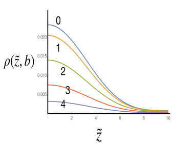
Figure 4: $\rho(\tilde{z},b)$. The numbers refer to the value of $b$ in units of GeV^-1.

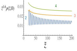
Figure 5: ${\tilde{z}}^{1.6}\rho({\tilde{z}},0)$. The numbers refer to the value of $\tau$, the number of constituents in the Fock state.

The main interest here is to study the dependence on ${\tilde{z}}$, which is displayed in Fig. 5 for $b=0$. The same general behavior is seen for other values of $b$. The density falls roughly as $1/{\tilde{z}}^{1.6}$. This very slow falloff that again indicates the large spatial extent of hadronic wave functions.

We examine how the transverse extent depends on ${\tilde{z}}$ by defining an expectation value $b^{2}_{\tau}({\tilde{z}})\equiv{\int d^{2}b\left|\psi_{\tau}({\tilde{z}},b)\right|^{2}b^{2}\over\int d^{2}b\left|\psi_{\tau}({\tilde{z}},b)\right|^{2}}.$ The values shown in Fig. 6 generally increase with increasing ${\tilde{z}}$, in contrast with intuition based on rotational invariance.

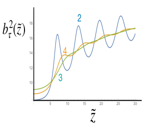
Figure 6: $b^{2}_{\tau}(\tilde{z})$ in units of GeV^-2. The numbers refer to the value of $\tau$, the number of constituents in the Fock state.

The unorthodox behavior shown in Fig. 6 motivates us to define the average value of ${\bf b}^{2}$ as a function of $x$: $b^{2}(x)\equiv\int d^{2}{b}b^{2}\left|\psi_{\it eff}(x,\mathbf{b})\right|^{2}={4f\over(1-x)^{2}}.$ This quantity is independent of the value of $\tau$ and ranges from about 1.1 fm² at $x=0$ to 0.23 fm² at $x=1$. This decreasing behavior arises from the vanishing of $f(x)$ as $x$ approaches 1. Indeed $\lim_{x\to 1}f(x)\,{\rm GeV}^{2}=1.27454(1-x)^{2}+0.416245(1-x)^{3}+\cdots$. The mean-square transverse size decreases with increasing $x$. Similarly, the mean-square transverse momentum $k^{2}(x)=1/b^{2}(x)$ increases with increasing $x$. This behavior is completely opposite to that obtained from the simpler form of Eq. (11), as well as that of many models of GPDs.

Summary and Outlook

A longitudinal spatial variable ${\tilde{z}}$ has been introduced in Eq. (4), thus allowing a representation of light-front wave functions in terms of all three frame-independent spatial coordinate variables. Both the valence model of Eq. (11) and the universal light-front model which incorporates Regge behavior Eq. (21) provide a light front coordinate-space density, Eq. (13), that has a long tail in the longitudinal separation between the struck constituent and the spectators. This allows the absorption-emission separation distance, $x^{-}$ occurring in deep inelastic scattering to be very large. The result Eq. (10) shows how given regions of $x^{-}$ contribute to the quark distribution at each value of Bjorken $x$.

Acknowledgments This work has been partially supported by U.S. D. O. E. Grant No. DE-FG02-97ER-41014 and by U.S. D. O. E. contract. No. DE–AC02–76SF00515. SLAC-PUB-17497. We thank T. Liu, R. Suffian, A. Radyushkin, D. Richards and J. Qiu for useful discussions.

References

- (1) D. Muller, D. Robaschik, B. Geyer, F.-M. Dittes and J. Horejsi, Fortsch. Phys. 42, 101 (1994) doi:10.1002/prop.2190420202 [hep-ph/9812448].
- (2) X. D. Ji, Phys. Rev. Lett. 78, 610 (1997) doi:10.1103/PhysRevLett.78.610 [hep-ph/9603249].
- (3) A. V. Radyushkin, Phys. Lett. B 380, 417 (1996) doi:10.1016/0370-2693(96)00528-X [hep-ph/9604317].
- (4) D. E. Soper, “The Parton Model And The Bethe-Salpeter Wave Function,” Phys. Rev. D 15, 1141 (1977).
- (5) M. Burkardt, “Impact parameter space interpretation for generalized parton distributions,” Int. J. Mod. Phys. A 18, 173 (2003) [hep-ph/0207047].
- (6) G. A. Miller, “Charge Density of the Neutron,” Phys. Rev. Lett. 99, 112001 (2007) [arXiv:0705.2409 [nucl-th]].
- (7) G. A. Miller, “Transverse Charge Densities,” Ann. Rev. Nucl. Part. Sci. 60, 1 (2010) [arXiv:1002.0355 [nucl-th]].
- (8) P. A. M. Dirac, “Forms Of Relativistic Dynamics,” Rev. Mod. Phys. 21, 392 (1949).
- (9) G. P. Lepage and S. J. Brodsky, “Exclusive Processes In Perturbative Quantum Chromodynamics,” Phys. Rev. D 22, 2157 (1980).
- (10) S. J. Brodsky, H. C. Pauli and S. S. Pinsky, “Quantum chromodynamics and other field theories on the light cone,” Phys. Rept. 301, 299 (1998) [arXiv:hep-ph/9705477].
- (11) S. J. Brodsky and G. P. Lepage, “Exclusive Processes And The Exclusive Inclusive Connection In Quantum Chromodynamics,” SLAC-PUB-2294 (1979).
- (12) S. J. Brodsky, D. S. Hwang, B. Q. Ma and I. Schmidt, “Light-cone representation of the spin and orbital angular momentum of relativistic composite systems,” Nucl. Phys. B 593, 311 (2001) [arXiv:hep-th/0003082].
- (13) J. C. Collins and D. E. Soper, “Parton Distribution and Decay Functions,” Nucl. Phys. B 194, 445 (1982).
- (14) X. D. Ji, “Off forward parton distributions,” J. Phys. G 24, 1181 (1998) [hep-ph/9807358].
- (15) J. C. Collins, “What exactly is a parton density?,” Acta Phys. Polon. B 34, 3103 (2003) [hep-ph/0304122].
- (16) M. Tanabashi et al. [Particle Data Group], “Review of Particle Physics,” Phys. Rev. D 98, 030001 (2018).
- (17) X. Ji, “Parton Physics on a Euclidean Lattice,” Phys. Rev. Lett. 110, 262002 (2013) doi:10.1103/PhysRevLett.110.262002 [arXiv:1305.1539 [hep-ph]].
- (18) C. Alexandrou, K. Cichy, M. Constantinou, K. Jansen, A. Scapellato and F. Steffens, “Light-Cone Parton Distribution Functions from Lattice QCD,” Phys. Rev. Lett. 121, no. 11, 112001 (2018) [arXiv:1803.02685 [hep-lat]].
- (19) H. W. Lin et al., “Proton Isovector Helicity Distribution on the Lattice at Physical Pion Mass,” Phys. Rev. Lett. 121, no. 24, 242003 (2018) doi:10.1103/PhysRevLett.121.242003 [arXiv:1807.07431 [hep-lat]].
- (20) R. S. Sufian, J. Karpie, C. Egerer, K. Orginos, J. W. Qiu and D. G. Richards, Phys. Rev. D 99, no. 7, 074507 (2019) doi:10.1103/PhysRevD.99.074507 [arXiv:1901.03921 [hep-lat]].
- (21) K. Cichy and M. Constantinou, “A guide to light-cone PDFs from Lattice QCD: an overview of approaches, techniques and results,” Adv. High Energy Phys. 2019, 3036904 (2019) [arXiv:1811.07248 [hep-lat]].
- (22) C. Monahan, “Recent Developments in -dependent Structure Calculations,” PoS LATTICE 2018, 018 (2018) [arXiv:1811.00678 [hep-lat]].
- (23) V. N. Gribov, B. L. Ioffe and I. Y. Pomeranchuk, “What is the range of interactions at high-energies,” Sov. J. Nucl. Phys. 2, 549 (1966) [Yad. Fiz. 2, 768 (1965)].
- (24) B. L. Ioffe, “Space-time picture of photon and neutrino scattering and electroproduction cross-section asymptotics,” Phys. Lett. 30B, 123 (1969).
- (25) Y. V. Kovchegov and E. Levin, “Quantum chromodynamics at high energy,” Camb. Monogr. Part. Phys. Nucl. Phys. Cosmol. 33, 1 (2012).
- (26) V. Braun, P. Gornicki and L. Mankiewicz, “Ioffe - time distributions instead of parton momentum distributions in description of deep inelastic scattering,” Phys. Rev. D 51, 6036 (1995)
- (27) V. Braun and D. Muller, “Exclusive processes in position space and the pion distribution amplitude,” Eur. Phys. J. C 55, 349 (2008)
- (28) R. L. Jaffe, Nucl. Phys. B 229, 205 (1983).
- (29) M. Diehl, “Generalized parton distributions,” Phys. Rept. 388, 41 (2003)
- (30) A. V. Radyushkin, Phys. Rev. D 96, no. 3, 034025 (2017) doi:10.1103/PhysRevD.96.034025 [arXiv:1705.01488 [hep-ph]].
- (31) K. Orginos, A. Radyushkin, J. Karpie and S. Zafeiropoulos, “Lattice QCD exploration of parton pseudo-distribution functions,” Phys. Rev. D 96, no. 9, 094503 (2017) doi:10.1103/PhysRevD.96.094503 [arXiv:1706.05373 [hep-ph]].
- (32) A. Dumitru, G. A. Miller and R. Venugopalan, “Extracting many-body color charge correlators in the proton from exclusive DIS at large Bjorken x,” Phys. Rev. D 98, no. 9, 094004 (2018) [arXiv:1808.02501 [hep-ph]].
- (33) A. Accardi et al., “Electron Ion Collider: The Next QCD Frontier : Understanding the glue that binds us all,” Eur. Phys. J. A 52, no. 9, 268 (2016) [arXiv:1212.1701 [nucl-ex]].
- (34) P. Hoyer, “Comments on the Relativity of Shape,” AIP Conf. Proc. 904, no. 1, 65 (2007)
- (35) S. J. Brodsky and G. F. de Teramond, Phys. Rev. D 77, 056007 (2008)
- (36) S. J. Brodsky, G. F. de Teramond, H. G. Dosch and J. Erlich, “Light-Front Holographic QCD and Emerging Confinement,” Phys. Rept. 584, 1 (2015) [arXiv:1407.8131 [hep-ph]].
- (37) G. F. de Teramond et al. [HLFHS Collaboration], “Universality of Generalized Parton Distributions in Light-Front Holographic QCD,” Phys. Rev. Lett. 120, no. 18, 182001 (2018) [arXiv:1801.09154 [hep-ph]].
- (38) S. J. Brodsky, G. F. de T’eramond, H. G. Dosch and C. Lorce, “Universal Effective Hadron Dynamics from Superconformal Algebra,” Phys. Lett. B 759, 171 (2016) [arXiv:1604.06746 [hep-ph]].
- (39) G. F. de Teramond and S. J. Brodsky, “Gauge/Gravity Duality and Strongly Coupled Light-Front Dynamics,” PoS LC 2010, 029 (2010) doi:10.22323/1.119.0029 [arXiv:1010.1204 [hep-ph]].
- (40) S. J. Brodsky, D. Chakrabarti, A. Harindranath, A. Mukherjee and J. P. Vary, “Hadron optics in three-dimensional invariant coordinate space from deeply virtual Compton scattering,” Phys. Rev. D 75, 014003 (2007) [arXiv:hep-ph/0611159].