The Spectral Bias of the Deep Image Prior

Abstract

The “deep image prior” proposed by Ulyanov et al. [9] is an intriguing property of neural nets: a convolutional encoder-decoder network can be used as a prior for natural images. The network architecture implicitly introduces a bias; If we train the model to map white noise to a corrupted image, this bias guides the model to fit the true image before fitting the corrupted regions. This paper explores why the deep image prior helps in denoising natural images. We present a novel method to analyze trajectories generated by the deep image prior optimization and demonstrate: (i) convolution layers of the an encoder-decoder decouple the frequency components of the image, learning each at different rates (ii) the model fits lower frequencies first, making early stopping behave as a low pass filter. The experiments study an extension of Cheng et al. [2], which showed that at initialization the deep image prior is equivalent to a stationary Gaussian process.

1 Introduction

It is well known that large neural nets have the capacity to overfit training data, even fitting random labels perfectly [12]. Arpit et al. [1] confirmed this, but showed that networks learn "simple patterns" first. This may explain why these models, despite their capacity, generalize well with early stopping. [4, 3, 8, 5]. One way to formalize the notion of a simple pattern is to observe the frequency components of the function learned by the model. Simple patterns are smooth, composed of low frequencies. A number of works use this approach to describe the bias induced by deep networks. For example, [11, 10] study the F-principle which states that the models first learn the low-frequency components when fitting a signal. Rahaman et al. [6] demonstrated a similar spectral bias of a deep fully-connected network with ReLU activation.

The Deep Image Prior (DIP) considers the following setup. Let $f_{\theta}:\mathcal{X}\to\mathcal{X^{\prime}}$ be a convolutional encoder-decoder parameterized by $\theta\in\Theta$. $\mathcal{X}$, $\mathcal{X^{\prime}}$ are spaces of $D$ dimensional signals. DIP studies the following optimization: $\min\limits_{\theta}||f_{\theta}(z)-x_{0}||^{2}$ where, $z\in\mathcal{X}$ is a fixed $D$ dimensional white noise vector. $N$ steps of gradient descent for this optimization traces out a trajectory in the parameter space: $\theta^{(1)},...\theta^{(N)}$. This has a corresponding trajectory $T$ in the output space $\mathcal{X^{\prime}}$: $f_{\theta^{(1)}}(z),...,f_{\theta^{N}}(z)$. Given enough capacity and suitable learning rate scheme, for a large $N$, the model will perfectly fit the signal, i.e., $f_{\theta^{N}}(z)=x_{0}$. For image denoising $\mathcal{X}$, $\mathcal{X^{\prime}}$ are spaces of all images ($D=2$) and $x_{0}=x^{*}+\eta$ is a noisy image: a clean image $x^{*}$ with added Gaussian noise $\eta$. Experiments in [9] show that early stopping with gradient descent will lead to denoised the image. In other words, the trajectory $T$ will contain a point that is close to the clean image $x^{*}$.

We use the spectral bias of the network to explain this denoising behavior. It is known that at initialization the generated output of the DIP is drawn from distribution that is approximately a stationary Gaussian process with smooth covariance function [2]. The experiments presented here suggest that this trend continues throughout the optimization, i.e., the model learns to construct the image from low to high frequencies. Thus, early stopping prevents fitting the high frequency components introduced by the additive Gaussian noise. The source code to reproduce results is available online.

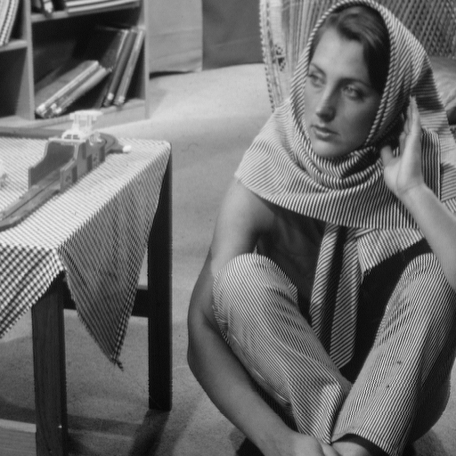
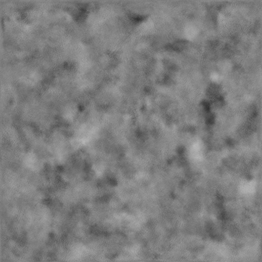
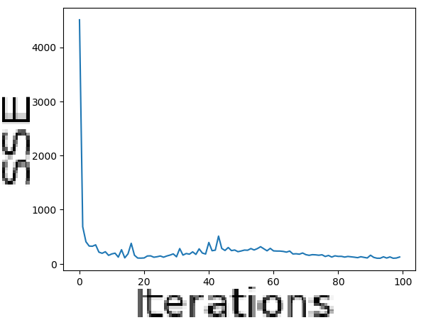
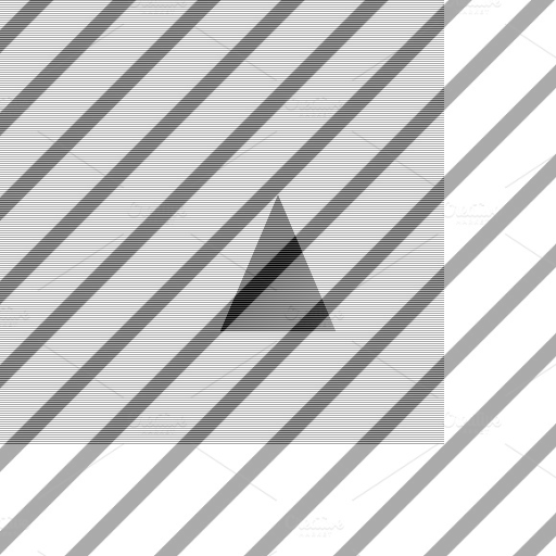
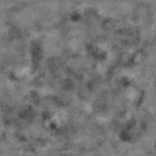
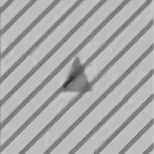
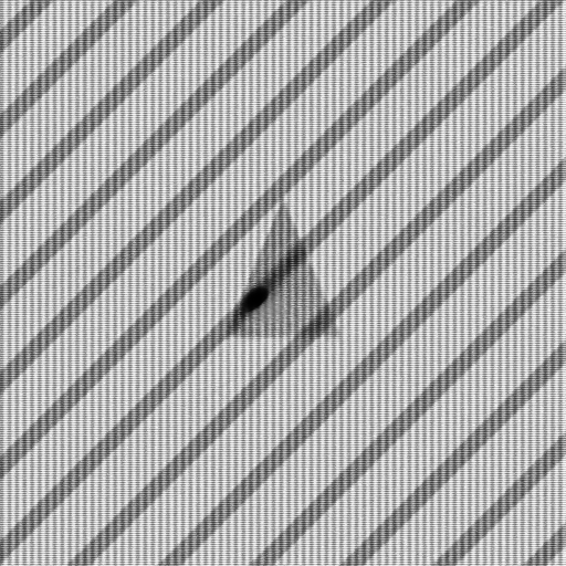
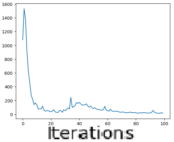
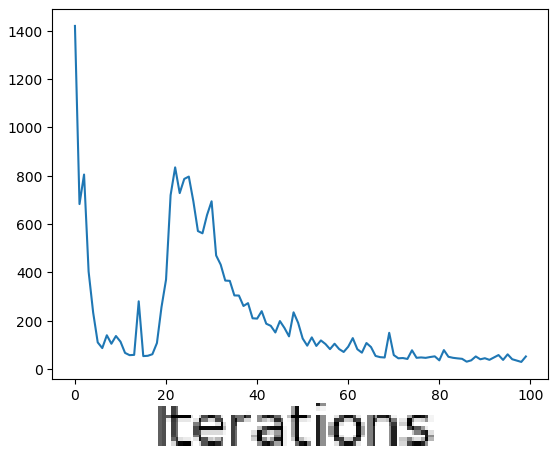
(a)	(b)	(c)	(d)	(e)	(f)	(g)	(h)

Figure 1: (a-e) DIP applied to two clean images. (a) Input images. (b) Initial output. (c) Output at the first convergence of trajectories. (d) Output at the second convergence of trajectories. (e) Variation of $\varepsilon$ across iterations. (f-g) Controlled amounts of high frequency patterns on triangle.png. Trajectories diverge more when the pattern covers a larger area. (Please zoom in for details.)

2 The Spectral Bias of the Deep Image Prior

We first demonstrate the spectral bias of the DIP in the exact setting as Ulyanov et al. [9]. Using the same model, i.e., a 5-layered convolutional autoencoder with $128$ channels each, the DIP optimization was run on clean images which have a range of frequency components, as shown in Figure 1(a). For each image, the optimization was run twice to generate trajectories $T_{1}$, $T_{2}$ in the output space. Let $\mathcal{\varepsilon}$ be the variation of the sum of squared error (SSE) between trajectories: $\mathcal{\varepsilon}^{(i)}=\sum\big{(}T_{1}^{(i)}-T_{2}^{(i)}\big{)}^{2}$.

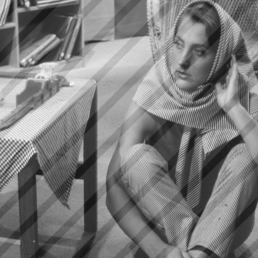
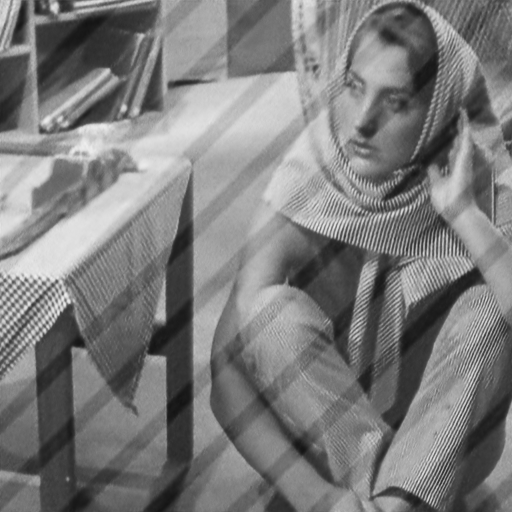
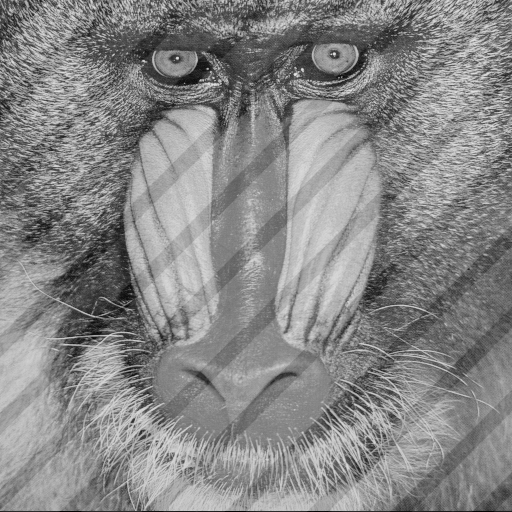
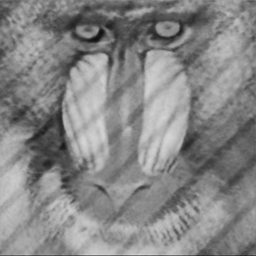
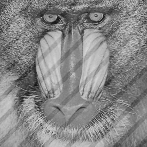
(a)	(b)	(c)

Figure 2: Some failure cases for the DIP. (a) Images with low frequency noise. (b) $20$ iterations: the model fits the noise, not the true high frequency components. (c) $500$ iterations: the model fits the signal perfectly.

Fig. 1 tracks the $\mathcal{\varepsilon}$ on two images: barbara.png naturally has high frequency components while triangle.png is a smooth image with a high frequency pattern superimposed on it. We observe the following:

• The initial output of the model is smooth (Fig. 1b). This is consistent with the analysis in [2], which showed that at initialization the output can be approximated as a draw from a stationary Gaussian process with a smooth covariance function.

• The trajectories converge twice (Fig. 1e). At the first point of convergence, the model predicts a low frequency reconstruction of the image (Fig. 1c). After the second converge, the model fits the high frequency components (Fig. 1d).

• Controlled amounts of the high frequency pattern were added to triangle.png. As it covers a larger spatial extent, the trajectories diverge more (Fig. 1(f-h)). This suggests that the reason for divergence corresponds to the model learning the higher frequencies.

These observations show that the model learns the frequency components of the image at different rates, fitting the low frequencies first (see Appendix A). Thus, early stopping is similar to low-pass filtering in the frequency domain.

The denoising experiments in [9] used additive Gaussian noise. Early stopping with DIP prevents fitting these, predicting the clean image before fitting the noise. We can now construct samples where deep image prior is guaranteed to fail. Low frequency noise is added to barbara.png and baboon.png: images which naturally have high frequencies, as shown in Fig. 2. After $20$ iterations, the model fits the noise, but not the high frequency components and goes on the fit the input perfectly after $500$ iterations. Thus, there is no point at which the model predicts the clean image. This strongly suggests that the ability of DIP to denoise images is brought about due to the frequency bias.

3 What causes the frequency bias?

Here we investigate what elements of the DIP lead to the aforementioned frequency bias in learning. In particular we show that both convolutions and upsampling introduce a bias.

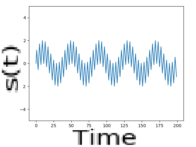
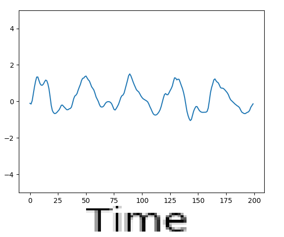
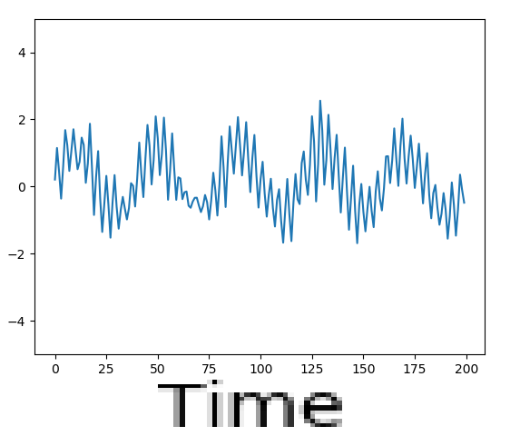
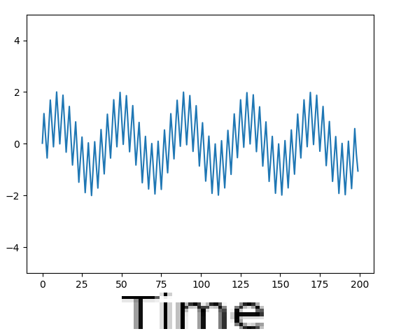
(a)	(b)	(c)	(d)
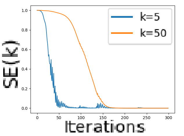
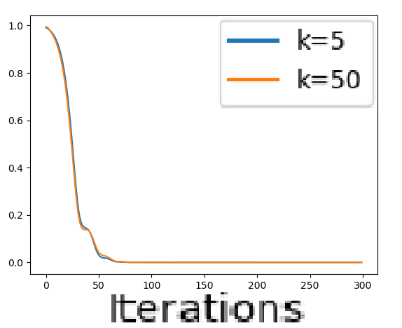
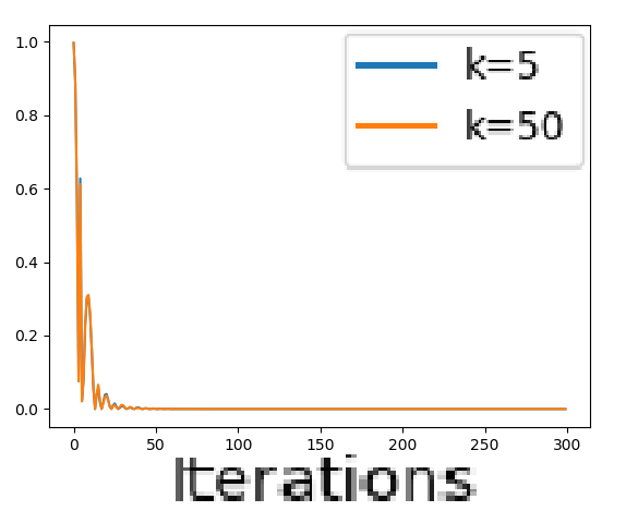
(e)	(f)	(g)	(h)

Figure 3: DIP on 1D signals. (a-e) Outputs of a model with conv layers. (a) Input signal (b) Predicted signal when $k_{1}$ converges, (c) when $k_{2}$ converges and (d) at the end of the optimization. (e) Variation of squared errors $SE(k_{1})$ and $SE(k_{2})$ across iterations. (f-h) Outputs of a model with linear layers. Variation of $SE(k_{1})$ and $SE(k_{2})$ with (f) 256 nodes per layers (g) 4096 nodes per layers (h) depth 24. This model fails to decouple frequencies.

3.1 Convolution Layers

The frequency selectiveness of a convolutional network architecture was shown in [7]. DIP uses a convolutional encoder-decoder. Here, we demonstrate using a simple experiment that the convolution layers of this architecture decouple the frequencies of the signal, fitting each at different rates. This does not happen if the encoder-decoder has only linear layers. Consider DIP on 1D signals, where $x_{0}=\sin(2\pi k_{1}t)+\sin(2\pi k_{2}t)$. The signal with $k_{1}=5$ and $k_{2}=50$ is shown in fig. 3(a). We run the DIP optimization on this signal and track the squared error $SE(k_{i})=(\tilde{A_{i}}-A_{i})^{2}$, where $\tilde{A_{i}}$ is the predicted amplitude and $A_{i}$ is the true amplitude for frequency $k_{i}$. We say that a frequency $k_{i}$ has converged at $t_{i}$ if $SE(k_{i})\leq\delta$ after $t_{i}$ iterations ($\delta=0.01$ for these experiments). This is similar to Experiment 1 in [6]. We compare the use of convolutions against linear layers in the model:

• DIP-Conv. A 10-layered encoder-decoder with 1D convolution layers, 256 channels. The variation in $SE(k_{1})$ and $SE(k_{2})$ is shown in Fig. 3(e). $SE(k_{1})$ drops sharply, leading $k_{1}$ to converge at 45 iterations. $k_{2}$ is learned slowly, converging at 151 iterations. Observing the predictions after each component converges (Fig. 3(b,c)), we see when $k_{1}$ converges, the model predicts a smooth reconstruction of the signal. Clearly, the frequency components are learned at different rates.

• DIP-Linear. The convolution layers of the DIP-conv were replaced with 256 unit linear layers (fully-connected) and the optimization was run again. Fig. 3(f) shows the results. The error for both frequencies drop at the same rate. The model never predicts a low-frequency reconstruction of the signal. Further, the lack of decoupling remains if we change the depth or width of the network (Fig. 3(g,h)) which suggests that it is intrinsic to linear layers and not related to the model capacity.

DIP	DIP Linear-128	DIP Linear-2048	ReLUNet
27.47	20.54	19.17	27.58

Table 1: Denoising performance. Only models with frequency bias are effective at denoising.

Effect on image denoising. To confirm that the above results extend to 2D signals, the same architecture variations were applied to images. DIP: Standard DIP for images using the model from [9] (similar to DIP-Conv above); DIP Linear-128: An encoder-decoder with 5 fully-connected layers, $128$ units each; DIP Linear-2048: DIP Linear, with $2048$ units each per layer (higher capacity); ReLUNet: A 10-layered fully-connected network with $256$ nodes per layer and ReLU activations to model images as signals. The model is trained to map pixel coordinates to the corresponding intensities (this will exhibit frequency bias as shown in [6]).

The ReLUNet and DIP-Linear architectures do not explicitly have convolution layers. However, their behavior is closely related to special cases of the DIP model. A ReLUNet predicts individual pixels without using neighborhood information, similar to a convolutional encoder-decoder with a kernel size of 1. DIP-Linear is similar to the other extreme, when the kernel size equals the size of the entire signal.

These models were used to fit images used in [9, 2] from a standard dataset. For efficiency, the images were downsampled by a factor of $4$. The entire trajectories in the output space were saved to see if they contain the denoised image (samples in Appendix D). To eliminate the effect of a badly chosen stopping time, we track the PSNR across the entire trajectory and record the best.

Table 1 shows the mean PSNR across 9 images (See appendix C for results per image). DIP performs the best, with ReLUNets achieving comparable performance. Encoder-decoders with only fully-connected layers perform significantly worse, irrespective of capacity, as they do not decouple frequencies. These results reinforce the idea that the denoising ability is a result of the frequency bias.

3.2 Upsampling Layers

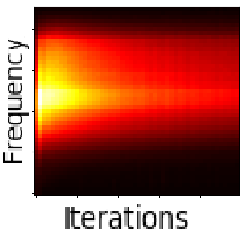
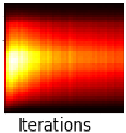
(a)	(b)
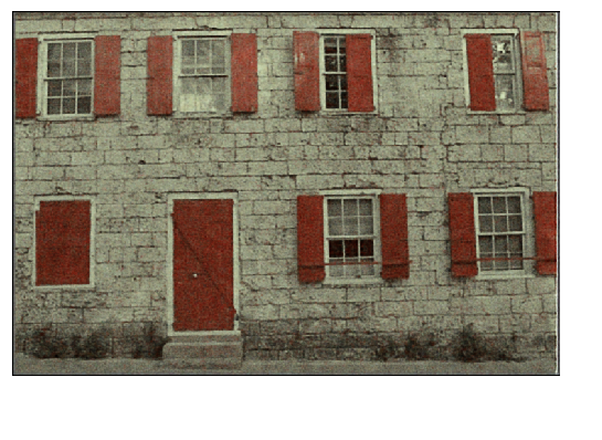
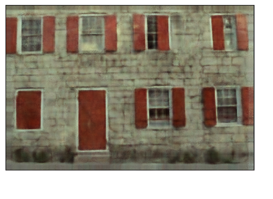
(c)	(d)

Figure 4: (a-b) Error in the power spectrum across the first $500$ iterations using (a) stride=$4$ and (b) stride=$32$. (c-d) Output at $500$ iterations with (c) stride=$4$ and (d) stride=$32$. A larger stride produces a smoother output at the same iteration.

Two types of upsampling methods were explored in [9]: nearest neighbor and bilinear. Both methods can be viewed as upsampling with zeros followed by a convolution with a fixed smoothing kernel. These strongly bias the model towards smooth images. For example, upsampling a 1D signal with stride $L$, the frequency responses of the associated convolution operations are ${\sin(\pi Lk)}/{\pi Lk}$ for nearest-neighbor. and ${\sin^{2}(\pi Lk)}/{\pi^{2}Lk^{2}}$ for bilinear upsampling (Appendix E). The responses decay with frequency and stride. This is qualitatively demonstrated in Fig. 4. The low error region of the power spectrum (dark region at the bottom of Fig. 4(a,b)) grows more slowly, with a higher stride.

4 Conclusion

This paper studies the DIP, proposing an explanation for the denoising experiments presented in [9]. We associate the phenomenon with the notion of frequency bias: convolutional networks fit the low frequencies of a signal first. Experiments on 1D signals and images with additive Gaussian noise strongly suggest that this is the causative factor behind the denoising behavior observed in DIP.

5 Appendix

A Power Spectrum in Experiment 1

Fig. 5 shows the trajectory in Exp. 1 Fig. 1) and the corresponding power spectrum. This clearly shows the frequency components growing from low to high frequencies.

Figure 5: The power spectrum of DIP output on clean images. Iterations $20$, $40$, $60$, $80$ and $200$ for (a) barbara.png and (b) triangle.png. (Please zoom in to see the patterns clearly.)

B Effect of model capacity

We study the effect of changing the model capacity in the experiments with 1D signals with 2 frequency components (Section 3.1). The depth and width of the model was varied, keeping all other settings fixed. For each capacity, we record the mean and standard deviation of the time to convergence for each frequency component across $10$ runs.

Fig. 6(a,b) show the results when the model uses only convolution layers. We observe the following:

• Increasing the depth makes the model separate frequencies more. In Fig. 6(a), as the depth increases, the mean convergence time for $k_{2}$ increases much faster than that for $k_{1}$, indicating that the model fits the higher frequency more slowly.

• Increasing the width (number of channels per layer) leads to faster convergence for both frequencies (fig. 6(b)). The convergence time of $k_{2}$ drops faster, eventually becoming lower than that of $k_{1}$ ($1280$ channels per layer generally fits the higher frequency first).

These results suggest that a deep, narrow model will be more effective at decoupling frequencies than a wide, shallow one. Fig. 6(c,d) show the results when the model uses only fully-connected layers. The overall trend is the same as that of the convolutional model: time to convergence increases with depth and decreases with width. However, both frequency components converge at the same time. This supports the conclusion that fully-connected layers are unable to decouple frequencies.

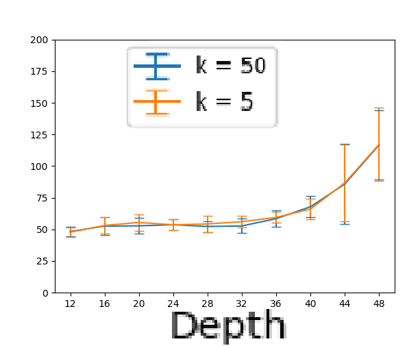
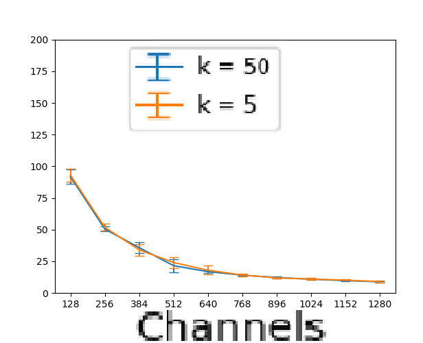
(a)	(b)	(c)	(d)

Figure 6: Effect of varying capacity on the convergence time of frequency components $k_{1}$ and $k_{2}$. (a-b) Results with convolution layers: convergence time with (a) increasing depth (b) increasing number of channels per layer. (c-d) Results with linear layers: convergence time with (c) increasing depth (d) increasing number of nodes per hidden layer.

C Detailed Denoising Results

Denoising results on each image using the architectures in section 3.1. Table 1 summarizes the table below, showing the means per column.

Image	DIP	DIP Linear-128	DIP Linear-2048	ReLUNet
Baboon	24.73$\pm$0.04	20.48$\pm$0.06	20.35$\pm$0.43	24.56$\pm$0.02
F16	27.00$\pm$0.15	20.72$\pm$0.12	18.60$\pm$1.85	26.67$\pm$0.14
House	26.89$\pm$0.10	20.69$\pm$0.04	18.89$\pm$1.45	27.21$\pm$0.22
kodim01	25.90$\pm$0.08	20.35$\pm$0.07	20.54$\pm$0.07	25.95$\pm$0.07
kodim02	29.20$\pm$0.13	20.74$\pm$0.01	20.59$\pm$0.19	29.99$\pm$0.09
kodim03	29.26$\pm$0.13	20.47$\pm$0.04	18.13$\pm$0.13	29.62$\pm$0.16
kodim12	29.61$\pm$0.06	20.36$\pm$0.03	17.74$\pm$0.04	29.63$\pm$0.16
Lena	27.49$\pm$0.06	20.48$\pm$0.01	18.67$\pm$0.72	27.78$\pm$0.16
Peppers	27.12$\pm$0.11	20.60$\pm$0.01	18.98$\pm$1.31	26.82$\pm$0.16

Table 2: Per-image denoising performance. Mean and standard deviation of the PSNR across $5$ runs.

D Trajectories of denoising experiment

Fig. 7 shows samples from the trajectories while denoising with DIP (fig. 7(a)) and with a ReLUNet (fig. 7(b)). The input image is House.png, downsampled by a factor of $4$ (to $128$x$128$) with added Gaussian noise. Both models demostrate frequency bias and predict the clean image before fitting the noise. The samples also show the difference between the DIP and ReLUNet models. ReLUNets are extremely biased towards smooth images, taking much longer to fit the higher frequencies: the DIP model starts fitting the noise at $500$ iterations, while the ReLUNet model does so at $50000$ iterations (even then, the model doesn’t fit these components perfectly, predicting a blurred version of the noise).

(a)	(b)

Figure 7: Samples from trajectories when denoising House.png small. (a) Output of DIP model at iterations $0$, $100$, $500$ (b) Output of ReLUNet model at iterations $0$, $10000$, $50000$

E Frequency response of upsampling methods

Standard upsampling methods can be viewed as upsampling by padding with zeros followed by a convolution with a fixed smoothing kernel $f(t)$. Let $\hat{f}(k)$ be the frequency response of this kernel (where $k$ is the frequency). Upsampling with zeros scales the image by a factor $L$, but adds high frequency components. These components are removed after convolution with $f(t)$ if $\hat{f}(k)$ decays with frequency. The spatial extent of $f(t)$ is the upsampling stride $L$. For example, in 1D, these kernels are as follows:

• For nearest neighbor, the kernel is the box function: $f(t)=\begin{cases}1&\text{if}t\in[\frac{-L}{2},\frac{L}{2}]\\ 0&\text{otherwise}\end{cases}$
  The frequency response of this kernel is: $\hat{f}(k)=\frac{\sin(\pi Lk)}{\pi Lk}$

• For bilinear upsampling, the kernel is the triangle wave function: $f(t)=\begin{cases}1-|t|&\text{if}|t|\leq\frac{L}{2}\\ 0&\text{otherwise}\end{cases}$
  The frequency response of this kernel is: $\hat{f}(k)=\frac{\sin^{2}(\pi Lk)}{L\pi^{2}k^{2}}$

Clearly, both favor low frequency components, with the bilinear having a stronger bias ($\propto\frac{1}{k^{2}}$) than nearest neighbor ($\propto\frac{1}{k}$).

References

- [1] D. Arpit, S. Jastrzebski, N. Ballas, D. Krueger, E. Bengio, M. S. Kanwal, T. Maharaj, A. Fischer, A. Courville, Y. Bengio, et al. A closer look at memorization in deep networks. In Proceedings of the 34th International Conference on Machine Learning-Volume 70, pages 233–242. JMLR. org, 2017.
- [2] Z. Cheng, M. Gadelha, S. Maji, and D. Sheldon. A bayesian perspective on the deep image prior. arXiv preprint arXiv:1904.07457, 2019.
- [3] S. Gunasekar, J. D. Lee, D. Soudry, and N. Srebro. Implicit bias of gradient descent on linear convolutional networks. In Advances in Neural Information Processing Systems, pages 9461–9471, 2018.
- [4] B. Neyshabur, S. Bhojanapalli, D. McAllester, and N. Srebro. Exploring generalization in deep learning. In Advances in Neural Information Processing Systems, pages 5947–5956, 2017.
- [5] B. Neyshabur, R. Tomioka, and N. Srebro. In search of the real inductive bias: On the role of implicit regularization in deep learning. arXiv preprint arXiv:1412.6614, 2014.
- [6] N. Rahaman, D. Arpit, A. Baratin, F. Draxler, M. Lin, F. A. Hamprecht, Y. Bengio, and A. Courville. On the spectral bias of deep neural networks. arXiv preprint arXiv:1806.08734, 2018.
- [7] A. M. Saxe, P. W. Koh, Z. Chen, M. Bhand, B. Suresh, and A. Y. Ng. On random weights and unsupervised feature learning. In ICML, volume 2, page 6, 2011.
- [8] D. Soudry, E. Hoffer, M. S. Nacson, S. Gunasekar, and N. Srebro. The implicit bias of gradient descent on separable data. The Journal of Machine Learning Research, 19(1):2822–2878, 2018.
- [9] D. Ulyanov, A. Vedaldi, and V. Lempitsky. Deep image prior. In Proceedings of the IEEE Conference on Computer Vision and Pattern Recognition, pages 9446–9454, 2018.
- [10] Z.-Q. J. Xu, Y. Zhang, T. Luo, Y. Xiao, and Z. Ma. Frequency principle: Fourier analysis sheds light on deep neural networks. arXiv preprint arXiv:1901.06523, 2019.
- [11] Z.-Q. J. Xu, Y. Zhang, and Y. Xiao. Training behavior of deep neural network in frequency domain. arXiv preprint arXiv:1807.01251, 2018.
- [12] C. Zhang, S. Bengio, M. Hardt, B. Recht, and O. Vinyals. Understanding deep learning requires rethinking generalization. arXiv preprint arXiv:1611.03530, 2016.