Linear response of a superfluid Fermi gas inside its pair-breaking continuum

Abstract

We study the signatures of the collective modes of a superfluid Fermi gas in its linear response functions for the order-parameter and density fluctuations in the Random Phase Approximation (RPA). We show that a resonance associated to the Popov-Andrianov (or sometimes “Higgs”) mode is visible inside the pair-breaking continuum at all values of the wavevector $q$, not only in the (order-parameter) modulus-modulus response function but also in the modulus-density and density-density responses. At nonzero temperature, the resonance survives in the presence of thermally broken pairs even until the vicinity of the critical temperature $T_{c}$, and coexists with both the Anderson-Bogoliubov modes at temperatures comparable to the gap $\Delta$ and with the low-velocity phononic mode predicted by RPA near $T_{c}$. The existence of a Popov-Andrianov-“Higgs” resonance is thus a robust, generic feature of the high-energy phenomenology of pair-condensed Fermi gases, and should be accessible to state-of-the-art cold atom experiments.

I Introduction

A primary way to probe the collective mode spectrum of a many-body system is by measuring the response functions of its macroscopic observables such as its density, or, in the case of a condensed system, its order parameter. These response functions can be measured by driving the system at a given wavenumber $q$ and varying the drive frequency $\omega$. In the theoretical case where the collective mode is undamped, one expects a infinitely narrow resonance (a Dirac peak) when $\omega$ coincides with the collective mode frequency $\omega_{\mathbf{q}}$. However, in most systems, collective modes are coupled to one or several continua of excitations, for example by intrinsic couplings to other elementary excitations. The system response in this case is less abrupt: the response functions are nonzero at all frequencies $\omega$ belonging to the continuum and the Dirac peak of the collective mode is replaced, in the favorable cases, by a broadened resonance. Theoretically, this damped resonance can be related to the existence of a pole in the analytic continuation of the response functions through their branch cuts associated to the continua Fetter and Walecka (1971); Nozières (1963); Cohen-Tannoudji et al. (1988). Eventually, if the coupling to the continuum is very strong, the resonance may entirely disappear, such that only a slowly varying response remains visible inside the continuum.

Superfluid Fermi gases, which one can form by cooling down fermionic atoms prepared in two internal states $\uparrow/\downarrow$ Greiner et al. (2003); Zwierlein et al. (2003); Jochim et al. (2003); Zwierlein et al. (2005); Joseph et al. (2007); Schirotzek et al. (2008); Nascimbène et al. (2010); Ku et al. (2012); Sidorenkov et al. (2013); Hoinka et al. (2017), offer a striking example of this fundamental many-body phenomenon. This system of condensed pairs of $\uparrow/\downarrow$ fermions is described by 3 collective fields: the total density $\rho$ of particles and the phase and modulus of the order-parameter $\Delta$. In the general case, the fluctuations of those 3 fields are coupled and the collective modes have components on all of them. The system has also fermionic quasiparticles describing the breaking of pairs into unpaired fermions Bardeen et al. (1957); Haussmann (1993); Haussmann et al. (2009); Van Loon et al. (2020), and two fermionic continua of quasiparticle biexcitations: a gapped quasiparticle-quasiparticle continuum and a gapless quasiparticle-quasihole continuum (to which the collective modes are coupled only at nonzero temperature). Since the coupling to these continua is not small in general, the collective mode spectrum can be obtained only after nonperturbative analytic continuations Schmid and Schön (1975); Andrianov and Popov (1976); Kurkjian et al. (2019); Klimin et al. (2019). Performing an analytic continuation to study collective modes coupled to a continuum is a powerful heuristic tool: it is indispensable to interpret the shape of the response functions in terms of collective phenomena and to define precisely the spectrum of the collective branches. However, the poles found in the analytic continuation are not directly observable and one should always relate them to resonances which experiments can measure in the response functions.

Meanwhile, the experimental study of the collective modes of a superfluid Fermi gas is a very active field of research Joseph et al. (2007); Hoinka et al. (2017); Patel et al. (2019), with a special focus on the high-energy collective modes Behrle et al. (2018) (at $\omega$ larger than the quasiparticle-quasiparticle continuum threshold at $2\Delta$) where a branch with quadratic dispersion Andrianov and Popov (1976); Kurkjian et al. (2019) is expected, reminiscent of the Higgs modes in high-energy physics Pekker and Varma (2015), superconductors Sooryakumar and Klein (1980); Matsunaga et al. (2013); Méasson et al. (2014); Cea et al. (2015); Grasset et al. (2018, 2019), superfluid fermionic Helium Volovik and Zubkov (2014) and nuclear matter Abrosimov et al. (2011, 2014). This motivates us to discuss the observability, in the order-parameter and density response functions of the gas, of the collective modes predicted by Ref. Andrianov and Popov (1976); Kurkjian et al. (2019); Castin and Kurkjian (2019); Klimin et al. (2019) based on the analytic structure of the functions continuated to imaginary frequencies. There are two major obstacles Cea et al. (2015); Tsuchiya et al. (2013); Pekker and Varma (2015) to the observation of the Popov-Andrianov-“Higgs” resonance in a conventional fermionic condensate. $(i)$ So far the resonance has been clearly identified only in the modulus-modulus response function, whereas experiments (both in superconductors Pekker and Varma (2015) and ultracold Fermi gases Hoinka et al. (2017); Patel et al. (2019)) usually excite or measure the density of the fermions. $(ii)$ In a conventional fermionic condensate, where the resonance energy is above $2\Delta$ and the resonance broadened by its coupling to the pair-breaking continuum, it is generally not known whether a quality factor and spectral weight large enough to allow for an observation can be reached. Most studies then look for situations where the damping by the continuum is absent, as in Charged-Density-Wave superconductors Sooryakumar and Klein (1980); Méasson et al. (2014); Cea et al. (2015); Grasset et al. (2018, 2019), inhomogeneous systems Bruun (2014) or superfluids in unconventional lattice geometries Tsuchiya et al. (2013). Here, we show that the resonance is observable in the density-density and density-modulus response functions at strong coupling. In those density responses, the spectral weights of the resonance tends to zero with the wavevector $q$ while the quality factor decreases when $q$ increases. Nevertheless we could identify an intermediary regime ($q\approx\sqrt{2m\mu}$ at unitarity) where the resonance, and the characteristic quadratic dependence on $q$ of its peak frequency, should be resolvable from the continuum background in an ultracold Fermi gas.

We study the response functions in Anderson’s Random Phase Approximation (RPA) Anderson (1958). We use the formulation of Ref. Kurkjian and Tempere (2017) in terms of bilinear quasiparticle operators that we generalize to nonzero temperature and to the presence of external drive fields. The RPA captures the coupling of the collective modes to the two fermionic continua (and the corresponding broadening of the resonances in the response functions) but neglects other couplings, in particular to the continua of two Beliaev (1958), three Landau and Khalatnikov (1949); Kurkjian et al. (2017) or more collective excitations. We show that in this approximation, the density fluctuations are sensitive to the fluctuations of $\Delta$, so that both modulus and phase collective modes are visible in the density response, but that the converse is not true. We give explicit expressions of each element of the response function matrix Fetter and Walecka (1971); Wong and Takada (1988); Bruun and Mottelson (2001); Minguzzi et al. (2001), and show that they agree with path-integral based treatments He (2016); Klimin et al. (2019).

As the spectrum and response-function signatures of the low-energy collective modes is known in the RPA at zero Anderson (1958); Marini et al. (1998); Combescot et al. (2006), nonzero temperature Kulik et al. (1981); Kurkjian and Tempere (2017) and near the critical temperature $T_{c}$ Andrianov and Popov (1976); Ohashi and Takada (1997); Klimin et al. (2019), we concentrate here on the high-energy ($\omega>2\Delta$) modes. At zero temperature, we show that the resonance of the Popov-Andrianov-“Higgs” mode is visible not only in the modulus-modulus response Kurkjian et al. (2019) but also as a global extremum (in the region $\omega>2\Delta$) in the modulus-phase and modulus-density responses, and as a local extremum in the density-density response at strong coupling. As suggested by the analytic structure found in Ref. Castin and Kurkjian (2019), we show that the branch remains observable at large $q$ (in particular at $q\approx\sqrt{2m\mu}$ in the weak-coupling limit $\Delta\ll\mu$) with a quality factor below, but not much below unity.

At nonzero temperature, where the RPA captures the thermal population of the fermionic quasiparticle branches (and only of those branches) and describes the collective modes in the collisionless approximation, we show that the Popov-Andrianov resonance is not destroyed by the presence of thermally excited fermionic quasiparticles. On the contrary, the increase of temperature (which reduces $\Delta$) favours the observability of the resonance in the density response functions by increasing the resonance spectral weight. The shape of the resonance is weakly affected by temperature, and for the order-parameter responses this shape is actually the same as at zero temperature for a slightly different interaction strength. Close to the critical temperature $T_{c}$, we show that collective mode in the pair-breaking continuum branch is not hidden by the low-velocity phononic branch Klimin et al. (2019) as long as $\hbar^{2}q^{2}/m\lesssim\Delta^{2}/\mu$. This is in contrast with the Anderson-Bogoliubov branch, which disappears near $T_{c}$ according to the RPA.

Altogether our findings confirm the observability of the Popov-Andrianov-“Higgs” branch, which appears, after our study, as the strongest feature of the high-energy phenomenology of pair-condensed Fermi gases. It is observable in wide ranges of values of the interaction strength, exciting wavevector and temperature, and it is only weakly affected by the singularities caused in the response functions by the structure changes of the fermionic continuum. We are then optimistic about its observability, especially if the experiments can access one of the modulus response functions (modulus-modulus, modulus-phase or modulus-density). The modulus of the order-parameter can be excited by a Feshbach modulation of the scattering length Gurarie (2009); Kurkjian et al. (2019), after which the modulus-density response can be measured by absorption images as in Ref. Hoinka et al. (2017); Patel et al. (2019). Alternatively the density can be excited by a Bragg pulse Hoinka et al. (2017) or by shaking the confinement walls Patel et al. (2019), and the order-parameter modulus measured after a bosonization of the Cooper pairs. In the density-density response, it would be interesting to see if the peak observed in Hoinka et al. (2017) above $2\Delta$ has the characteristic behavior of the Popov-Andrianov-“Higgs” mode, that is, a quadratic dependence on $q$ for both the peak frequency and its width.

II BCS theory at nonzero temperature

To derive the matrix of linear response functions, we use the formalism of Ref. Kurkjian and Tempere (2017), itself based on the RPA approach of Anderson Anderson (1958), and we generalize it to the presence of pairing and density exciting fields. We start by briefly recalling the formalism of BCS theory at nonzero temperature. In real and momentum space, the Hamiltonian of an isolated gas of fermions in two internal states $\sigma=\uparrow/\downarrow$ with $s$-wave contact interactions is given by

$$\hat{H} = l^{3}\sum_{\mathbf{r},\sigma=\uparrow/\downarrow}\hat{\psi}_{\sigma}^{\dagger}(\mathbf{r})\left(-\frac{1}{2m}\Delta_{\mathbf{r}}-\mu\right)\hat{\psi}_{\sigma}(\mathbf{r})+g_{0}l^{3}\sum_{{\mathbf{r}}}\hat{\psi}_{\uparrow}^{\dagger}({\mathbf{r}})\hat{\psi}_{\downarrow}^{\dagger}(\mathbf{r})\hat{\psi}_{\downarrow}(\mathbf{r}){\hat{\psi}_{\uparrow}}(\mathbf{r})$$ (1)

$$= \sum_{\mathbf{k}\in\mathcal{D},\sigma=\uparrow/\downarrow}\left(\frac{k^{2}}{2m}-\mu\right)\hat{a}_{\mathbf{k}\sigma}^{\dagger}\hat{a}_{\mathbf{k}\sigma}+\frac{g_{0}}{V}\sum_{\mathbf{k},\mathbf{k}^{\prime},\mathbf{q}\in\mathcal{D}}\hat{a}_{\mathbf{k}^{\prime}\uparrow}^{\dagger}\hat{a}_{-\mathbf{k}^{\prime}-\mathbf{q}\downarrow}^{\dagger}\hat{a}_{-\mathbf{k}-\mathbf{q}\downarrow}\hat{a}_{\mathbf{k}\uparrow}.$$ (2)

We use from now on the convention $\hbar=k_{\rm B}=1$. To introduce a momentum cutoff in a natural way, we discretize space into a cubic lattice of step $l$ and impose periodic boundary conditions (in a volume $V=L^{3}$), which restrict the values of the wavevectors to $\mathcal{D}=\frac{2\pi}{L}\mathbb{Z}^{3}\cap[-\pi/{l},\pi/{l}[^{3}$. The bare coupling constant $g_{0}$ is renormalized to reproduce the correct $s$-wave scattering length of the two-body problem:

$$\frac{1}{g_{0}}=\frac{m}{4\pi\hbar^{2}a}-\int_{[-\pi/l,\pi/l[^{3}}\frac{{d}^{3}k}{(2\pi)^{3}}\frac{m}{{k^{2}}}.$$ (3)

At the end of the calculation we take the lattice spacing $l$ to $0$, and thus $g_{0}$ tends to $0$ to compensate the divergence of the integral on the right-hand-side of (3).

BCS theory describes the equilibrium state at temperature $T$ by the Gaussian state:

$$\hat{\rho}_{\rm BCS}(T)=\frac{\exp\left(-\hat{H}_{\rm BCS}/T\right)}{\mathcal{Z}}$$ (4)

where $\mathcal{Z}$ is the partition function and the BCS Hamiltonian $H_{\rm BCS}$ is obtained by treating the interactions in the mean-field approximation, i.e. by replacing the quartic interaction term $g_{0}\hat{\psi}_{\uparrow}^{\dagger}({\mathbf{r}})\hat{\psi}_{\downarrow}^{\dagger}(\mathbf{r})\hat{\psi}_{\downarrow}(\mathbf{r})\hat{\psi}_{\uparrow}(\mathbf{r})$ in (2) by a quadratic one $\Delta(\hat{\psi}_{\uparrow}^{\dagger}({\mathbf{r}})\hat{\psi}_{\downarrow}^{\dagger}(\mathbf{r})+\textrm{cc})$, through the introduction of the self-consistent pairing-field

$$\Delta=g_{0}\left\langle\hat{\psi}_{\uparrow}^{\dagger}({\mathbf{r}})\hat{\psi}_{\downarrow}^{\dagger}(\mathbf{r})\right\rangle_{T}.$$ (5)

Here $\langle\ldots\rangle_{T}$ denotes the average in the thermal state $\hat{\rho}_{\rm BCS}(T)$. This quadratic Hamiltonian can be diagonalized easily into a Hamiltonian describing fermionic elementary excitations on top of a ground state energy $E_{0}$:

$$\hat{H}_{\rm BCS}=E_{0}+\sum_{\mathbf{k}\in\mathcal{D}}\epsilon_{\mathbf{k}}\hat{\gamma}_{\mathbf{k}\sigma}^{\dagger}\hat{\gamma}_{\mathbf{k}\sigma}.$$ (6)

Here the eigenenergy of a fermionic excitation is

$$\epsilon_{\mathbf{k}}=\sqrt{\xi_{\mathbf{k}}^{2}+\Delta^{2}}\quad\mbox{with}\quad\xi_{\mathbf{k}}=\frac{k^{2}}{2m}-\mu.$$ (7)

The fermionic quasiparticle operators $\hat{\gamma}_{\mathbf{k},\sigma}$ are obtain after a Bogoliubov rotation of the particle operators $\hat{a}_{\mathbf{k},\sigma}$ as in the zero temperature case:

$$\hat{{\gamma}}_{\mathbf{k}\uparrow} = U_{\mathbf{k}}\hat{a}_{\mathbf{k}\uparrow}+V_{\mathbf{k}}\hat{a}_{-\mathbf{k}\downarrow}^{\dagger}$$ (8)

$$\hat{{\gamma}}_{-\mathbf{k}\downarrow} = -V_{\mathbf{k}}\hat{a}_{\mathbf{k}\uparrow}^{\dagger}+U_{\mathbf{k}}\hat{a}_{-\mathbf{k}\downarrow}$$ (9)

with the Bogoliubov coefficients $U_{\mathbf{k}}$ and $V_{\mathbf{k}}$:

$$U_{\mathbf{k}}=\sqrt{1+\frac{\xi_{\mathbf{k}}}{\epsilon_{\mathbf{k}}}}\quad\mbox{and}\quad V_{\mathbf{k}}=\sqrt{1-\frac{\xi_{\mathbf{k}}}{\epsilon_{\mathbf{k}}}}.$$ (10)

The difference with the zero temperature case lies in the average values of the bilinear operators:

$$\langle\hat{a}^{\dagger}_{\mathbf{k},\sigma}\hat{a}_{\mathbf{k},\sigma}\rangle = \left(U_{\mathbf{k}}^{2}-V_{\mathbf{k}}^{2}\right)f_{\mathbf{k}}+V_{\mathbf{k}}^{2}$$ (11)

$$\langle\hat{a}_{-\mathbf{k},\downarrow}\hat{a}_{\mathbf{k},\uparrow}\rangle = -\left(1-2f_{\mathbf{k}}\right)U_{\mathbf{k}}V_{\mathbf{k}},$$ (12)

which now depend on the Fermi-Dirac occupation number

$$f_{\mathbf{k}}=\langle\hat{\gamma}^{\dagger}_{\mathbf{k},\sigma}\hat{\gamma}_{\mathbf{k},\sigma}\rangle_{T}=\frac{1}{1+\exp{\epsilon_{\mathbf{k}}/T}}.$$ (13)

This thermal population of the quasiparticle modes also affect the gap equation:

$$\Delta=-\frac{g_{0}}{L^{3}}\sum_{\mathbf{k}\in\mathcal{D}}U_{\mathbf{k}}V_{\mathbf{k}}(1-2f_{\mathbf{k}}).$$ (14)

Thus, at nonzero temperature, BCS theory captures the effects due to the thermally excited fermionic quasiparticles (the broken pairs); it completely neglects that there are also thermally excited collective modes (some of which are gapless) which is a serious limitation, particularly at strong coupling.

III RPA equations of motion in presence of drive fields

To study the linear response of the gas, we introduce, on top of the Hamiltonian (2) of the isolated gas, a quadratic Hamiltonian describing the experimental driving of the system:

$$\hat{H}_{\rm drive}=l^{3}\sum_{\mathbf{r}}\left(u_{\uparrow}(\mathbf{r},t)\hat{\psi}_{\uparrow}^{\dagger}(\mathbf{r})\hat{\psi}_{\uparrow}(\mathbf{r})+u_{\downarrow}(\mathbf{r},t)\hat{\psi}_{\downarrow}^{\dagger}(\mathbf{r})\hat{\psi}_{\downarrow}(\mathbf{r})+\left[\hat{\psi}^{\dagger}_{\uparrow}(\mathbf{r})\hat{\psi}^{\dagger}_{\downarrow}(\mathbf{r})\phi(\mathbf{r},t)+\mbox{c.c.}\right]\right).$$ (15)

Here the fields $u_{\sigma}(\mathbf{r})$, coupled to the density of spin $\sigma$ fermions, describe for instance a Bragg excitation of the gas Hoinka et al. (2017). The complex field $\phi(\mathbf{r})$ coupled to the quantum pairing field $\hat{\psi}^{\dagger}_{\uparrow}(\mathbf{r})\hat{\psi}^{\dagger}_{\downarrow}(\mathbf{r})$ can be imposed for instance by a Feshbach-modulation of the interaction strength Gurarie (2009). An excitation coupled to the phase of $\hat{\psi}^{\dagger}_{\uparrow}(\mathbf{r})\hat{\psi}^{\dagger}_{\downarrow}(\mathbf{r})$ can be achieved using a time- and space-dependent Josephson junction as proposed in Klimin et al. (2019). This drive Hamiltonian decomposes into a sum of Fourier components of the momentum $\mathbf{q}$ transferred to system:

$$\hat{H}_{\rm drive}=\sum_{\mathbf{q}}\hat{H}_{\rm drive}(\mathbf{q})\qquad\mbox{with}\qquad\hat{H}_{\rm drive}(\mathbf{q})=\sum_{\mathbf{k}}\left(u_{\uparrow}(-\mathbf{q})\hat{n}_{\mathbf{k}}^{\mathbf{q}}+u_{\downarrow}(-\mathbf{q})\hat{\bar{n}}_{\mathbf{k}}^{\mathbf{q}}\right)+\phi(-\mathbf{q})\sum_{\mathbf{k}}\hat{\bar{d}}_{\mathbf{k}}^{\mathbf{q}}+\bar{\phi}(-\mathbf{q})\sum_{\mathbf{k}}\hat{{d}}_{\mathbf{k}}^{\mathbf{q}}.$$ (16)

We use here Anderson’s Anderson (1958) notations for the bilinear fermion operators,

$$\hat{n}_{\mathbf{k}}^{\mathbf{q}} =\hat{a}_{\mathbf{k}+\mathbf{q}/2\uparrow}^{\dagger}\hat{a}_{\mathbf{k}-\mathbf{q}/2\uparrow} \hat{\bar{n}}_{\mathbf{k}}^{\mathbf{q}} =\hat{a}_{-\mathbf{k}+\mathbf{q}/2\downarrow}^{\dagger}\hat{a}_{-\mathbf{k}-\mathbf{q}/2\downarrow}$$

$$\hat{d}_{\mathbf{k}}^{\mathbf{q}} =\hat{a}_{-\mathbf{k}-\mathbf{q}/2\downarrow}\hat{a}_{\mathbf{k}-\mathbf{q}/2\uparrow} \hat{\bar{d}}_{\mathbf{k}}^{\mathbf{q}} =\hat{a}_{\mathbf{k}+\mathbf{q}/2\uparrow}^{\dagger}\hat{a}_{-\mathbf{k}+\mathbf{q}/2\downarrow}^{\dagger}$$ (17)

and the Fourier transforms of the drive fields:

$$u_{\sigma}(\mathbf{q}) = \frac{l^{3}}{V}\sum_{\mathbf{r}}{e}^{{i}\mathbf{q}\cdot\mathbf{r}}u_{\sigma}(\mathbf{r})$$ (18)

$$\phi(\mathbf{q}) = \frac{l^{3}}{V}\sum_{\mathbf{r}}{e}^{{i}\mathbf{q}\cdot\mathbf{r}}\phi(\mathbf{r})\quad\mbox{and}\quad\bar{\phi}(\mathbf{q})=\phi^{*}(-\mathbf{q}).$$ (19)

In the framework of linear response theory, we seek the response of the system to first order in the fields $\phi$ and $u_{\sigma}$. We thus neglect the quantum fluctuations in the terms of the equations of motion deriving from $\hat{H}_{\rm drive}$:

$$[\hat{a}\hat{b},\hat{H}_{\rm drive}]\simeq\left\langle[\hat{a}\hat{b},\hat{H}_{\rm drive}]\right\rangle_{T},$$ (20)

where the average value $\langle{[\hat{a}\hat{b},\hat{H}_{\rm drive}]}\rangle_{T}$ is taken in the BCS equilibrium state at zero fields. The rest of the derivation is similar to what is explained in Refs. Kurkjian (2016); Kurkjian and Tempere (2017): one writes the Heisenberg equations of motion for the bilinear fermionic operators (17) and linearizes them using incomplete Wick contractions (i.e the replacement $\hat{a}\hat{b}\hat{c}\hat{d}\rightarrow\hat{a}\hat{b}\langle\hat{c}\hat{d}\rangle_{T}+\langle\hat{a}\hat{b}\rangle_{T}\hat{c}\hat{d}-\hat{a}\hat{c}\langle\hat{b}\hat{d}\rangle_{T}-\langle\hat{a}\hat{c}\rangle_{T}\hat{b}\hat{d}+\ldots$). The resulting equations of motion of the bilinear particle operators are given in Appendix A. We give here the equations of motion in their simplest form, which is in the quasiparticle basis. At the level of the bilinear operators, the Bogoliubov rotation (8)–(9) becomes:

$$\begin{pmatrix}\hat{y}_{\mathbf{k}}^{\mathbf{q}}\\ \hat{h}_{\mathbf{k}}^{\mathbf{q}}\\ \hat{s}_{\mathbf{k}}^{\mathbf{q}}\\ \hat{m}_{\mathbf{k}}^{\mathbf{q}}\end{pmatrix}\equiv\begin{pmatrix}\hat{\gamma}_{-\mathbf{k}_{+},\downarrow}\hat{\gamma}_{\mathbf{k}_{-},\uparrow}-\hat{\gamma}_{\mathbf{k}_{+},\uparrow}^{\dagger}\hat{\gamma}_{-\mathbf{k}_{-},\downarrow}^{\dagger}\\ \hat{\gamma}_{\mathbf{k}_{+}\uparrow}^{\dagger}\hat{\gamma}_{\mathbf{k}_{-}\uparrow}-\hat{\gamma}_{-\mathbf{k}_{+}\downarrow}^{\dagger}\hat{\gamma}_{-\mathbf{k}_{-}\downarrow}\\ \hat{\gamma}_{-\mathbf{k}_{+},\downarrow}\hat{\gamma}_{\mathbf{k}_{-},\uparrow}+\hat{\gamma}_{\mathbf{k}_{+},\uparrow}^{\dagger}\hat{\gamma}_{-\mathbf{k}_{-},\downarrow}^{\dagger}\\ \hat{\gamma}_{\mathbf{k}_{+}\uparrow}^{\dagger}\hat{\gamma}_{\mathbf{k}_{-}\uparrow}+\hat{\gamma}_{-\mathbf{k}_{+}\downarrow}^{\dagger}\hat{\gamma}_{-\mathbf{k}_{-}\downarrow}\\ \end{pmatrix}=\begin{pmatrix}W_{\mathbf{k}\mathbf{q}}^{+}&w_{\mathbf{k}\mathbf{q}}^{-}&0&0\\ -w_{\mathbf{k}\mathbf{q}}^{-}&W_{\mathbf{k}\mathbf{q}}^{+}&0&0\\ 0&0&W_{\mathbf{k}\mathbf{q}}^{-}&-w_{\mathbf{k}\mathbf{q}}^{+}\\ 0&0&w_{\mathbf{k}\mathbf{q}}^{+}&W_{\mathbf{k}\mathbf{q}}^{-}\\ \end{pmatrix}\begin{pmatrix}\hat{d}_{\mathbf{k}}^{\mathbf{q}}-\hat{\bar{d}}_{\mathbf{k}}^{\mathbf{q}}\\ \hat{n}_{\mathbf{k}}^{\mathbf{q}}-\hat{\bar{n}}_{\mathbf{k}}^{\mathbf{q}}\\ \delta(\hat{d}_{\mathbf{k}}^{\mathbf{q}}+\hat{\bar{d}}_{\mathbf{k}}^{\mathbf{q}})\\ \delta(\hat{n}_{\mathbf{k}}^{\mathbf{q}}+\hat{\bar{n}}_{\mathbf{k}}^{\mathbf{q}})\\ \end{pmatrix},$$ (21)

where we have used $\mathbf{k}_{\pm}=\mathbf{k}\pm\mathbf{q}/2$, $W_{\mathbf{k}\mathbf{q}}^{\pm}=U_{\mathbf{k}_{+}}U_{\mathbf{k}_{-}}\pm V_{\mathbf{k}_{+}}V_{\mathbf{k}_{-}}$ and $w_{\mathbf{k}\mathbf{q}}^{\pm}=U_{\mathbf{k}_{+}}V_{\mathbf{k}_{-}}\pm V_{\mathbf{k}_{+}}U_{\mathbf{k}_{-}}$. Performing this change of basis on the equations of motion, we get:

$${i}\hbar\frac{{d}\hat{y}_{\mathbf{k}}^{\mathbf{q}}}{{d}t} =\epsilon_{\mathbf{k}\mathbf{q}}^{+}\hat{s}_{\mathbf{k}}^{\mathbf{q}}+(1-f_{\mathbf{k}_{+}}-f_{\mathbf{k}_{-}})\left[W_{\mathbf{k}\mathbf{q}}^{-}\left(\delta\hat{\Delta}^{\mathbf{q}}+\delta\hat{\bar{\Delta}}^{\mathbf{q}}+\phi_{+}(\mathbf{q})\right)-w_{\mathbf{k}\mathbf{q}}^{+}\left(g_{0}\left[\delta\hat{n}_{\uparrow}^{\mathbf{q}}+\delta\hat{{n}}_{\downarrow}^{\mathbf{q}}\right]+u_{+}(\mathbf{q})\right)\right]$$ (22)

$${i}\hbar\frac{{d}\hat{s}_{\mathbf{k}}^{\mathbf{q}}}{{d}t} =\epsilon_{\mathbf{k}\mathbf{q}}^{+}\hat{y}_{\mathbf{k}}^{\mathbf{q}}+(1-f_{\mathbf{k}_{+}}-f_{\mathbf{k}_{-}})\left[W_{\mathbf{k}\mathbf{q}}^{+}\left(\hat{\Delta}^{\mathbf{q}}-\hat{\bar{\Delta}}^{\mathbf{q}}+\phi_{-}(\mathbf{q})\right)-w_{\mathbf{k}\mathbf{q}}^{-}\left(g_{0}\left[\hat{n}_{\uparrow}^{\mathbf{q}}-\hat{{n}}_{\downarrow}^{\mathbf{q}}\right]-u_{-}(\mathbf{q})\right)\right]$$ (23)

$${i}\hbar\frac{{d}\hat{m}_{\mathbf{k}}^{\mathbf{q}}}{{d}t} =-\epsilon_{\mathbf{k}\mathbf{q}}^{-}\hat{h}_{\mathbf{k}}^{\mathbf{q}}-(f_{\mathbf{k}_{+}}-f_{\mathbf{k}_{-}})\left[w_{\mathbf{k}\mathbf{q}}^{-}\left(\hat{\Delta}^{\mathbf{q}}-\hat{\bar{\Delta}}^{\mathbf{q}}+\phi_{-}(\mathbf{q})\right)+W_{\mathbf{k}\mathbf{q}}^{+}\left(g_{0}\left[\hat{n}_{\uparrow}^{\mathbf{q}}-\hat{{n}}_{\downarrow}^{\mathbf{q}}\right]-u_{-}(\mathbf{q})\right)\right]$$ (24)

$${i}\hbar\frac{{d}\hat{h}_{\mathbf{k}}^{\mathbf{q}}}{{d}t} =-\epsilon_{\mathbf{k}\mathbf{q}}^{-}\hat{m}_{\mathbf{k}}^{\mathbf{q}}+(f_{\mathbf{k}_{+}}-f_{\mathbf{k}_{-}})\left[w_{\mathbf{k}\mathbf{q}}^{+}\left(\delta\hat{\Delta}^{\mathbf{q}}+\delta\hat{\bar{\Delta}}^{\mathbf{q}}+\phi_{+}(\mathbf{q})\right)+W_{\mathbf{k}\mathbf{q}}^{-}\left(g_{0}\left[\delta\hat{n}_{\uparrow}^{\mathbf{q}}+\delta\hat{{n}}_{\downarrow}^{\mathbf{q}}\right]+u_{+}(\mathbf{q})\right)\right],$$ (25)

where $\phi_{\pm}(\mathbf{q})=\phi(\mathbf{q})\pm\bar{\phi}(\mathbf{q})$, $u_{\pm}(\mathbf{q})=u_{\uparrow}(\mathbf{q})\pm u_{\downarrow}(\mathbf{q})$ and $\delta\hat{O}=\hat{O}-\langle\hat{O}\rangle_{T}$. At the linear order, the sole effect of the drive fields is thus to shift the collective quantities which enter in the equations of motion:

$$\hat{\Delta}^{\mathbf{q}} = \frac{g_{0}}{L^{3}}\sum_{\mathbf{k}_{1}}\hat{{d}}_{\mathbf{k}_{1}}^{\mathbf{q}}\quad\to\quad\hat{\Delta}^{\mathbf{q}}+\phi(\mathbf{q})$$ (26)

$$\hat{\bar{\Delta}}^{\mathbf{q}} = \frac{g_{0}}{L^{3}}\sum_{\mathbf{k}_{1}}\hat{\bar{d}}_{\mathbf{k}_{1}}^{\mathbf{q}}\quad\to\quad\hat{\bar{\Delta}}^{\mathbf{q}}+\bar{\phi}(\mathbf{q})$$ (27)

$$\hat{n}^{\mathbf{q}}_{\uparrow} = \frac{1}{L^{3}}\sum_{\mathbf{k}_{1}}\hat{n}_{\mathbf{k}_{1}}^{\mathbf{q}}\quad\to\quad\hat{n}^{\mathbf{q}}_{\uparrow}+u_{\downarrow}(\mathbf{q})/g_{0}$$ (28)

$$\hat{n}^{\mathbf{q}}_{\downarrow} = \frac{1}{L^{3}}\sum_{\mathbf{k}_{1}}\hat{\bar{n}}_{\mathbf{k}_{1}}^{\mathbf{q}}\quad\to\quad\hat{n}^{\mathbf{q}}_{\downarrow}+u_{\uparrow}(\mathbf{q})/g_{0}.$$ (29)

Note that one recovers the zero temperature system Eqs. (14–16) of Kurkjian and Tempere (2017) by setting $f_{\mathbf{k}}=0$ (in which case the equations of motion of the $\hat{\gamma}^{\dagger}\hat{\gamma}$ operators become trival).

IV Linear response to a periodic drive

IV.1 Matrix of response functions of a driven system

We now assume that the system is driven at a fixed frequency $\omega$, such that $\phi(\mathbf{r},t)=\phi(\mathbf{r}){e}^{{i}\omega t}$ and $u_{\sigma}(\mathbf{r},t)=u_{\sigma}(\mathbf{r}){e}^{{i}\omega t}$. We can then replace the time derivatives ${i}\hbar\partial_{t}$ in Eqs. (22–25) by $\omega+{i}0^{+}$. Rederiving with respect to time and resumming the system to form the collective quantities (26–29) yields the $4$-dimensional linear system

$$\left(\frac{V}{g_{0}}\mathbb{I}-\Pi(\omega,\mathbf{q})\right)\begin{pmatrix}2{i}\Delta\hat{\theta}^{\mathbf{q}}\\ 2\delta|\Delta^{\mathbf{q}}|\\ g_{0}\delta\hat{\rho}^{\mathbf{q}}\\ g_{0}\hat{p}^{\mathbf{q}}\end{pmatrix}=\Pi(\omega,\mathbf{q})\begin{pmatrix}\phi_{-}(\mathbf{q})\\ \phi_{+}(\mathbf{q})\\ u_{+}(\mathbf{q})\\ -u_{-}(\mathbf{q})\end{pmatrix},$$ (30)

where $\mathbb{I}$ is the identity matrix. We have introduced the density and polarisation fluctuations and reparametrized the fluctuations of the order-parameter as:

$$\hat{\Delta}^{\mathbf{q}} = (\Delta+\delta|\Delta^{\mathbf{q}}|){e}^{{i}\hat{\theta}^{\mathbf{q}}}$$ (31)

$$\hat{\bar{\Delta}}^{\mathbf{q}} = (\Delta+\delta|\Delta^{\mathbf{q}}|){e}^{-{i}\hat{\theta}^{\mathbf{q}}}$$ (32)

$$\hat{\rho}^{\mathbf{q}} = \hat{n}^{\mathbf{q}}_{\uparrow}+\hat{n}^{\mathbf{q}}_{\downarrow}$$ (33)

$$\hat{p}^{\mathbf{q}} = \hat{n}^{\mathbf{q}}_{\uparrow}-\hat{n}^{\mathbf{q}}_{\downarrow}.$$ (34)

We treat the phase $\hat{\theta}^{\mathbf{q}}$ of the order-parameter as an infinitesimal and therefore linearize the exponential in (31)–(32), which is consistent with our symmetry-breaking approach where the expansion is done around the mean-field state with a real $\Delta$. The system’s linear response matrix Fetter and Walecka (1971); Wong and Takada (1988); Bruun and Mottelson (2001); Minguzzi et al. (2001), which relates the fluctuations of the density and order-parameter to the infinitesimal drive fields, is then

$$\chi=\frac{\Pi}{\frac{V}{g_{0}}\mathbb{I}-\Pi}.$$ (35)

To describe the experimental behavior of a driven system, one usually concentrates on the imaginary part of $\chi$, which describes the energy absorbed by the system Fetter and Walecka (1971) (whereas the real part describes the energy refracted or reflected by the system).

The matrix $\chi$ is expressed in terms of the $4\times 4$ matrix $\Pi$ of the pair correlation functions Ohashi and Griffin (2003), computed in the BCS thermal state (4):

$$\Pi=\begin{pmatrix}\Sigma_{W^{+}W^{+}}^{\epsilon}&\Sigma_{W^{-}W^{+}}^{\omega}&-\Sigma_{w^{+}W^{+}}^{\omega}&0\\ \Sigma_{W^{+}W^{-}}^{\omega}&\Sigma_{W^{-}W^{-}}^{\epsilon}&-\Sigma_{w^{+}W^{-}}^{\epsilon}&0\\ -\Sigma_{W^{+}w^{+}}^{\omega}&-\Sigma_{W^{-}w^{+}}^{\epsilon}&\Sigma_{w^{+}w^{+}}^{\epsilon}&0\\ 0&0&0&-\Sigma_{w^{-}w^{-}}^{\epsilon}\end{pmatrix}-\begin{pmatrix}S_{w^{-}w^{-}}^{\epsilon}&S_{w^{+}w^{-}}^{\omega}&S_{W^{-}w^{-}}^{\omega}&0\\ S_{w^{-}w^{+}}^{\omega}&S_{w^{+}w^{+}}^{\epsilon}&S_{W^{-}w^{+}}^{\epsilon}&0\\ S_{w^{-}W^{-}}^{\omega}&S_{w^{+}W^{-}}^{\epsilon}&S_{W^{-}W^{-}}^{\epsilon}&0\\ 0&0&0&-S_{W^{+}W^{+}}^{\epsilon}\end{pmatrix}$$ (36)

where we generalize the notations of Refs. Kurkjian (2016); Castin and Kurkjian (2019) :

$$\Sigma_{ab}^{\epsilon}(\omega,\mathbf{q})=\sum_{\mathbf{k}}\frac{\epsilon_{\mathbf{k}\mathbf{q}}^{+}a_{\mathbf{k}\mathbf{q}}b_{\mathbf{k}\mathbf{q}}(1-f_{\mathbf{k}_{+}}-f_{\mathbf{k}_{-}})}{\omega^{2}-(\epsilon_{\mathbf{k}\mathbf{q}}^{+})^{2}}\qquad \Sigma_{ab}^{\omega}(\omega,\mathbf{q})=\sum_{\mathbf{k}}\frac{\omega a_{\mathbf{k}\mathbf{q}}b_{\mathbf{k}\mathbf{q}}(1-f_{\mathbf{k}_{+}}-f_{\mathbf{k}_{-}})}{\omega^{2}-(\epsilon_{\mathbf{k}\mathbf{q}}^{+})^{2}}$$ (37)

$$S_{ab}^{\epsilon}(\omega,\mathbf{q})=\sum_{\mathbf{k}}\frac{\epsilon_{\mathbf{k}\mathbf{q}}^{-}a_{\mathbf{k}\mathbf{q}}b_{\mathbf{k}\mathbf{q}}(f_{\mathbf{k}_{+}}-f_{\mathbf{k}_{-}})}{\omega^{2}-(\epsilon_{\mathbf{k}\mathbf{q}}^{-})^{2}}\qquad S_{ab}^{\omega}(\omega,\mathbf{q})=\sum_{\mathbf{k}}\frac{\omega a_{\mathbf{k}\mathbf{q}}b_{\mathbf{k}\mathbf{q}}(f_{\mathbf{k}_{+}}-f_{\mathbf{k}_{-}})}{\omega^{2}-(\epsilon_{\mathbf{k}\mathbf{q}}^{-})^{2}}.$$ (38)

Here $a$ and $b$ are one of the functions $W^{+}$, $W^{-}$, $w^{+}$ or $w^{-}$ of $\mathbf{k}$ and $\mathbf{q}$, and $\epsilon_{\mathbf{k}\mathbf{q}}^{+}$ is short-hand for $\epsilon_{\mathbf{k}+\mathbf{q}/2}\pm\epsilon_{\mathbf{k}-\mathbf{q}/2}$. The first and second matrix in the right-hand side of (36) are the contribution of respectively the quasiparticle-quasiparticle and quasiparticle-quasihole continua to $\Pi$. In our unpolarized system, the polarization fluctuations $\hat{n}_{\uparrow}^{\mathbf{q}}-\hat{{n}}_{\downarrow}^{\mathbf{q}}$ are entirely decoupled from the other collective fields. Note that the response functions computed here for a driven system also give access, through a Laplace transform Castin and Kurkjian (2019), to the time response following a perturbation localized in time.

Remark that, up to some signs, the matrix $\Pi$ has a tensor-product structure when expressed in terms of the vector $(a_{1},a_{2},a_{3},a_{4})=(W^{+},W^{-},w^{+},w^{-})$:

$$\Pi_{ij}=\begin{cases}\eta_{ij}\Sigma_{a_{i},a_{j}}^{\epsilon}-\eta\textquoteright_{ij}S_{a_{5-i},a_{5-j}}^{\epsilon}\quad\mbox{if}\quad i=j\quad\mbox{or}\quad i=5-j\\ \eta_{ij}\Sigma_{a_{i},a_{j}}^{\omega}-\eta\textquoteright_{ij}S_{a_{5-i},a_{5-j}}^{\omega}\quad\mbox{else}\end{cases}$$ (39)

The signs $\eta_{ij}=\pm 1$ and $\eta\textquoteright_{ij}=\pm 1$ should be read on Eq. (36).

IV.2 Eigenenergies of the collective modes

The response of the system should diverge when the drive frequency coincides with the eigenfrequency $\omega_{\mathbf{q}}$ of a collective mode; to find those eigenfrequencies, one should thus search for the poles of $\chi$, in other words the zero of its denominator:

$$\mbox{det}\left(\frac{V}{g_{0}}\mathbb{I}-\Pi(z_{\mathbf{q}},\mathbf{q})\right)=0.$$ (40)

When $\Pi$ has a branch cut on the real axis (which occurs for all $\omega\in\mathbb{R}$ at nonzero temperature and for $|\omega|>\min_{\mathbf{k}}(\epsilon_{\mathbf{k}+\mathbf{q}/2}+\epsilon_{\mathbf{k}-\mathbf{q}/2})$ at zero temperature), this equation cannot have a real solution. Its analytic continuation to the lower-half complex plane may however have solutions describing damped collective modes. Numerical and analytic methods to continue the matrix $\Pi$ through its branch cuts have been described in Kurkjian et al. (2019); Klimin et al. (2019); Castin and Kurkjian (2019).

IV.3 Explicit expressions of the response functions in the limit $g_{0}\to 0$

In the limit of zero lattice spacing ($l\to 0$), $g_{0}$ tends to $0$, $\Pi_{11}$ and $\Pi_{22}$ are equivalent to $V/g_{0}$, while $\Pi_{33}$ and $\Pi_{44}$ have a finite limit. We thus have the equivalences

$$\Pi\underset{g_{0}\to 0}{\sim}\begin{pmatrix}V/g_{0}&\Pi_{12}&\Pi_{13}&0\\ \Pi_{12}&V/g_{0}&\Pi_{23}&0\\ \Pi_{13}&\Pi_{23}&\Pi_{33}&0\\ 0&0&0&\Pi_{44}\end{pmatrix},\qquad\Pi-\frac{V}{g_{0}}\mathbb{I}\underset{g_{0}\to 0}{\sim}\begin{pmatrix}\Pi_{11}-V/g_{0}&\Pi_{12}&\Pi_{13}&0\\ \Pi_{12}&\Pi_{22}-V/g_{0}&\Pi_{23}&0\\ \Pi_{13}&\Pi_{23}&-V/g_{0}&0\\ 0&0&0&-V/g_{0}\end{pmatrix}.$$ (41)

Note that $\Pi_{11}-V/g_{0}$ and $\Pi_{22}-V/g_{0}$ have a finite limit when $g_{0}\to 0$. The determinant of the denominator of $\chi$ is then proportional to the determinant of the $2\times 2$ upper left submatrix:

$$\mbox{det}\left(\Pi-\frac{V}{g_{0}}\mathbb{I}\right)\underset{g_{0}\to 0}{\sim}\left(\frac{V}{g_{0}}\right)^{2}\mathcal{D}\qquad\mbox{with}\qquad\mathcal{D}={\left(\Pi_{11}-V/g_{0}\right)\left(\Pi_{22}-V/g_{0}\right)-\left(\Pi_{12}\right)^{2}}.$$ (42)

Physically this means that the collective mode spectrum is entirely determined by the (modulus and phase) fluctuations of the order-parameter. However, the density responses may exhibit collective mode resonances as a result of the density-order parameter couplings. Using the equivalences (41) to compute the matrix product in $\chi$ we obtain:

$$\tilde{\chi}\equiv\begin{pmatrix}1&0&0&0\\ 0&1&0&0\\ 0&0&V/g_{0}&0\\ 0&0&0&V/g_{0}\end{pmatrix}\chi\begin{pmatrix}g_{0}/V&0&0&0\\ 0&g_{0}/V&0&0\\ 0&0&1&0\\ 0&0&0&1\end{pmatrix}\underset{g_{0}\to 0}{\sim}-\frac{1}{\mathcal{D}}\\ \times\left(\begin{tabular}[]{cccc}$\tilde{\Pi}_{22}$&$-\Pi_{12}$&$\Pi_{13}\tilde{\Pi}_{22}-\Pi_{23}\Pi_{12}$&0\\ $-\Pi_{12}$&$\tilde{\Pi}_{11}$&$\Pi_{23}\tilde{\Pi}_{11}-\Pi_{13}\Pi_{12}$&0\\ \vspace{0.3cm} \text{{$({\Pi_{13}\tilde{\Pi}_{22}-\Pi_{12}\Pi_{23}})$}}&\text{{$({\Pi_{23}\tilde{\Pi}_{11}-\Pi_{13}\Pi_{12}})$}}&{\small$(\Pi_{13}^{2}\tilde{\Pi}_{22}+\Pi_{23}^{2}\tilde{\Pi}_{11}-2\Pi_{13}\Pi_{23}\Pi_{12}-\Pi_{33}\mathcal{D})$}&0\\ 0&0&0&$-\Pi_{44}\mathcal{D}$\end{tabular}\right).$$ (43)

We have used the notation $\tilde{\Pi}=\Pi-\frac{V}{g_{0}}$ and defined the response function matrix $\tilde{\chi}$ in the basis where all its coefficients are of order unity when $g_{0}\to 0$. For the density response functions we have in particular:

$$\tilde{\chi}_{13} = \frac{\Pi_{23}\Pi_{12}-\Pi_{13}\tilde{\Pi}_{22}}{\tilde{\Pi}_{11}\tilde{\Pi}_{22}-\Pi_{12}^{2}}$$ (44)

$$\tilde{\chi}_{23} = \frac{\Pi_{13}\Pi_{12}-\Pi_{23}\tilde{\Pi}_{11}}{\tilde{\Pi}_{11}\tilde{\Pi}_{22}-\Pi_{12}^{2}}$$ (45)

$$\tilde{\chi}_{33} = \frac{2\Pi_{13}\Pi_{23}\Pi_{12}-\Pi_{13}^{2}\tilde{\Pi}_{22}-\Pi_{23}^{2}\tilde{\Pi}_{11}}{\tilde{\Pi}_{11}\tilde{\Pi}_{22}-\Pi_{12}^{2}}+\Pi_{33},$$ (46)

which coincides with the explicit expressions obtained by Refs. He (2016); Klimin et al. (2019) in the path-integral formalism. At weak coupling ($\Delta/\mu\to 0$) and $q=O(\Delta)$, the modulus-phase and modulus-density matrix elements $\Pi_{12}$ and $\Pi_{23}$ vanish such that the collective modes are either pure modulus modes (if their eigenenergy solves $\Pi_{22}(z_{\mathbf{q}})-V/g_{0}=0$) or pure density-phase modes (if their eigenenergy solves $\Pi_{11}(z_{\mathbf{q}})-V/g_{0}=0$).

IV.4 Angular points of the response functions

We conclude this section by remarking that the response functions have the same angular points as the spectral density

$$\rho(\omega)=\frac{\Pi(\omega+{i}0^{+})-\Pi(\omega-{i}0^{+})}{-2{i}\pi}.$$ (47)

The quasiparticle-quasiparticle part of the spectral density (which originates from the first matrix in (36) with $\omega-(\epsilon_{\mathbf{k}+\mathbf{q}/2}+\epsilon_{\mathbf{k}-\mathbf{q}/2})$ in the denominator) is nonzero when the “pair-breaking” resonance condition is satisfied

$$\omega=\epsilon_{\mathbf{k}+\mathbf{q}/2}+\epsilon_{\mathbf{k}-\mathbf{q}/2}.$$ (48)

Physically, when this resonance condition is met, the drive field can break the pair of total momentum $\mathbf{q}$ into unpaired fermions of momenta $\mathbf{k}+\mathbf{q}/2$ and $\mathbf{k}-\mathbf{q}/2$. As a function of the increasing drive frequency $\omega$, this resonance condition is $(i)$ satisfied by no wavevector when $\omega<\omega_{1}$ (with $\omega_{1}=2\Delta$ at low-$q$), $(ii)$ satisfied for a connected set of wavevectors around the dispersion minimum of the quasiparticle branch for $\omega_{1}<\omega<\omega_{2}$, $(iii)$ satisfied by two connected sets of wavevectors, one in the increasing and one in the decreasing part of the BCS branch for $\omega_{2}<\omega<\omega_{3}$ and $(iv)$ satisfied for a connected set of wavevectors in the increasing part of the branch for $\omega>\omega_{3}$. These three boundary frequencies $\omega_{1}$, $\omega_{2}$ and $\omega_{3}$ will appear as angular points in the spectral function and therefore in the response functions. The quasiparticle-quasihole part of the spectral density (which originates from the second matrix in (36) with $\omega-(\epsilon_{\mathbf{k}+\mathbf{q}/2}-\epsilon_{\mathbf{k}-\mathbf{q}/2})$ in the denominator) is nonzero when the “absorption-emission” resonance condition is satisfied

$$\omega=\epsilon_{\mathbf{k}+\mathbf{q}/2}-\epsilon_{\mathbf{k}-\mathbf{q}/2}.$$ (49)

In this case, the drive field is not breaking the Cooper pairs but simply transferring more energy to the unpaired fermions already created by thermal agitation. This requires much less energy, which is why the quasiparticle-quasihole continuum is gapless. As a function of $\omega$, this resonance condition can be met on $(i)$ two disconnected sets of wavevectors, one in the increasing and one in the decreasing part of the BCS branch for $\omega<\omega_{\rm ph}$, $(ii)$ a single connected set of wavevectors in the increasing part of the branch for $\omega>\omega_{\rm ph}$. With $\omega_{\rm ph}$, we have found the four angular point of the response function $\omega\mapsto\chi(\omega)$ in $[0,+\infty[$.

V Long wavelength limit

In the long wavelength limit ($q\to 0$) the solutions of the collective mode equation (40) and the behavior of the response functions can be studied analytically. Below the pair-breaking continuum (at energies lower than $\min_{\mathbf{k}}(\epsilon_{\mathbf{k}+\mathbf{q}/2}+\epsilon_{\mathbf{k}-\mathbf{q}/2})$) the problem has been studied in-depth at zero and nonzero temperature. At zero temperature a real solution of (40) corresponding to the Anderson-Bogoliubov sound branch can be found Anderson (1958); Marini et al. (1998); Combescot et al. (2006). This branch appears as a pole in $\textrm{Re}\,\chi$ and as a Dirac peak in $\textrm{Im}\,\chi$ because the zero-temperature response functions are free of branch cuts below the pair-breaking continuum. This resonance was observed experimentally in the density-density response function by Bragg spectroscopy Hoinka et al. (2017) and in the low-$q$ limit it can be identified to hydrodynamic first sound Joseph et al. (2007); Sidorenkov et al. (2013); Patel et al. (2019). When the dispersion is supersonic (i.e. the function $q\mapsto\omega_{q}$ is convex) the resonance is broadened by intrinsic effects not captured by RPA Beliaev (1958); Kurkjian et al. (2017).

By contrast, the behavior of the response functions at high energy ($\omega>\min_{\mathbf{k}}(\epsilon_{\mathbf{k}+\mathbf{q}/2}+\epsilon_{\mathbf{k}-\mathbf{q}/2})$) is known in literature only at zero temperature. There, the collective mode equation (40) has a complex root departing quadratically with $q$ from $2\Delta$ Andrianov and Popov (1976), and the modulus-modulus response shows correspondingly a resonance at energies above $2\Delta$ Kurkjian et al. (2019). Here, we show analytically that (within the RPA) the same resonance exists at nonzero temperature, even until the vicinity of $T_{c}$. This result is somewhat in disagreement with Popov and Andrianov, who found no complex root close to $2\Delta$ in the limit $T\to T_{c}$.

V.1 General case

We first compute the matrix elements $\Pi_{ij}$ on the upper-half complex plane, that is for $\textrm{Im}\,z>0$. The long wavelength expansion can be perform using the method exposed in Kurkjian et al. (2019): since the energy is expected to depart quadratically from $2\Delta$, one parametrizes it as

$$z=2\Delta+\zeta\frac{\mu}{\Delta}\frac{q^{2}}{2m}.$$ (50)

The window $[2\Delta,\omega_{2}]$ between the first two angular points of the branch cut corresponds in the limit $q\to 0$ to $\zeta\in[0,1]$. With respect to the zero temperature case Kurkjian et al. (2019), the phase-phase and modulus-modulus matrix elements are simply multiplied by a factor $\mbox{tanh}(\Delta/2T)$:

$$\check{\Pi}_{11}(z,\mathbf{q}) \underset{q\to 0}{\sim} -\frac{\pi^{2}}{\check{q}}\mbox{tanh}\left(\frac{\Delta}{2T}\right)f_{11}(\zeta)\qquad\mbox{with}\qquad f_{11}(\zeta)={\mbox{ln}\frac{1+\sqrt{1-\zeta}}{\sqrt{\zeta}}+\frac{i\pi}{2}},$$ (51)

$$\check{\Pi}_{22}(z,\mathbf{q}) \underset{q\to 0}{\sim} {\pi^{2}\check{q}}\frac{\mu}{2\Delta}\mbox{tanh}\left(\frac{\Delta}{2T}\right)f_{22}(\zeta)\qquad\mbox{with}\qquad f_{22}(\zeta)={\sqrt{1-\zeta}-\zeta\mbox{ln}\frac{1+\sqrt{1-\zeta}}{\sqrt{\zeta}}-\frac{i\pi\zeta}{2}},$$ (52)

where we have introduced the dimensionless quantities $\check{q}=q/\sqrt{2m\Delta}$ and $\check{\Pi}_{ij}=\alpha(\Pi_{ij}-L^{3}/g_{0})$ for $(i,j)=(1,1)$ or $(2,2)$ and $\check{\Pi}_{ij}=\alpha\Pi_{ij}$ for the other matrix elements, the nondimensionalization factor $\alpha$ being $\Delta(2\pi/L\sqrt{2m\Delta})^{3}$. We have written the complex functions $f_{11}$ and $f_{22}$ of $\zeta$ in such a way that their spectral density (their imaginary part in the limit $\textrm{Im}\,\zeta\to 0^{+}$) is directly given by their last term. The modulus-phase matrix element is independent of $\zeta$ (it can be approximated by its value in $q=0$, $z=2\Delta$) but, unlike $\Pi_{11}$ and $\Pi_{22}$, depends on temperature through the two ratios $\Delta/T$ and $\mu/T$:

$$\check{\Pi}_{12}(z,\mathbf{q})\underset{q\to 0}{\sim}\check{\Pi}_{12}(2\Delta,0)={\pi^{2}}\sqrt{\frac{\mu}{2\Delta}}\mbox{tanh}\left(\frac{\Delta}{2T}\right)g_{12}\left(\frac{\mu}{T},\frac{\Delta}{T}\right),$$ (53)

where we have introduced the improper integral:

$${\pi^{2}}\sqrt{\frac{M}{2D}}\mbox{tanh}\left(\frac{D}{2}\right)g_{12}(M,D)=-\pi\mathcal{P}\int_{-M/D}^{\infty}\frac{d\xi\sqrt{\xi+{M}/{D}}}{\xi\sqrt{\xi^{2}+1}}\mbox{tanh}\frac{D\sqrt{\xi^{2}+1}}{2}.$$ (54)

Note that the quasiparticle-quasihole integrals (38) have been negligible in deriving expressions (51–53).

To find a root of the collective mode equation (40), one analytically continues $\Pi_{11}$ and $\Pi_{22}$ (and hence the determinant of $\Pi$) from upper to lower half-complex plane (the forms given in Eqs. (51)–(52) are in fact already analytic for $\mbox{Re}\,\zeta\in[0,1]$). The equation (40) for the complex collective mode frequency $z_{q}=2\Delta+\zeta_{s}\frac{\mu}{\Delta}\frac{q^{2}}{2m}+O(q^{3})$ becomes an explicit (yet transcendental) equation for the reduced frequency $\zeta_{s}$

$$f_{11}(\zeta_{s})f_{22}(\zeta_{s})+g_{12}^{2}\left(\frac{\mu}{T},\frac{\Delta}{T}\right)=0.$$ (55)

At zero temperature, this equation was derived in Andrianov and Popov (1976) in the weak-coupling limit and Kurkjian et al. (2019) in the general case. In this low-$q$ limit, the only dependence on temperature is through the $\zeta$-independent second term of (55).

V.2 Close to the phase transition

Unlike in the phononic regime ($q\to 0$ with $z=cq$) Klimin et al. (2019), no dramatic phenomenon occurs for the collective mode of the pair-breaking continuum when $T$ tends to the critical temperature $T_{c}$. We recall that in the RPA, the limit of the phase transition from the superfluid phase corresponds to

$$\frac{\Delta}{T} \to 0$$ (56)

$$\frac{\mu}{T} = \frac{\mu(T_{c})}{T_{c}}+O\left(\frac{\Delta}{T}\right)^{2}.$$ (57)

The RPA also assumes an infinite fermionic quasiparticle lifetime and thus describes the collective modes and their damping by the fermionic continua in the collisionless approximation.

The function $g_{12}$ tends to a finite nonzero constant in the limit $T\to T_{c}$:

$$g_{12}\left(\frac{\mu}{T},\frac{\Delta}{T}\right)\underset{T\to T_{c}}{\to}g_{12,c}\left(\frac{\mu_{c}}{T_{c}}\right)\equiv-\frac{{2}}{\pi}\sqrt{\frac{2T_{c}}{\mu_{c}}}\mathcal{P}\int_{-\mu_{c}/T_{c}}^{+\infty}\frac{\mbox{tanh}\frac{|e|}{2}\sqrt{e+\frac{\mu_{c}}{T_{c}}}de}{e|e|},$$ (58)

where we denote $\mu_{c}\equiv\mu(T_{c})$. In fact, the resonance near $T_{c}$ for a given value of $1/k_{\rm F}a$ has exactly the same shape as the $T=0$ resonance for a lower value (corresponding to weaker-coupling) of $1/k_{\rm F}a$. Using an equation-of-state to relate $1/k_{\rm F}a$ to both $\mu_{c}/T_{c}$ and $\mu(T=0)/\Delta(T=0)$ Klimin et al. (2019), the corresponding values $a_{0}$ and $a_{c}$ of the scattering length at $T=0$ and $T_{c}$ are found by solving:

$$g_{12,c}\left(\frac{\mu_{c}}{T_{c}}\Big{|}_{a=a_{c}}\right)=\lim_{T\to 0}g_{12}\left(\frac{\mu}{\Delta}\Big{|}_{a=a_{0}}\frac{\Delta}{T},\frac{\Delta}{T}\right).$$ (59)

Finally, the explicit expressions of the response functions in the long wavelength limit, at arbitrary $0\leq T<T_{c}$, and in the limit $T\to T_{c}$ are:

$$\!\!\!\!\!\!\!\!\!\chi_{11}(z,\mathbf{q}) = -\frac{\check{q}}{\pi^{2}\mbox{tanh}\frac{\Delta}{2T}}\frac{f_{22}(\zeta)}{f_{11}(\zeta)f_{22}(\zeta)+g_{12}^{2}(\mu/T,\Delta/T)}+O(q^{2})\underset{T\to T_{c}}{\sim}-\frac{2\check{q}}{\pi^{2}}\frac{T_{c}}{\Delta}\frac{f_{22}(\zeta)}{f_{11}(\zeta)f_{22}(\zeta)+g_{12,c}^{2}(\mu_{c}/T_{c})}$$ (60)

$$\!\!\!\!\!\!\!\!\!\chi_{22}(z,\mathbf{q}) = \frac{1}{\check{q}\pi^{2}\mbox{tanh}\frac{\Delta}{2T}}\frac{2\Delta}{\mu}\frac{f_{11}(\zeta)}{f_{11}(\zeta)f_{22}(\zeta)+g_{12}^{2}(\mu/T,\Delta/T)}+O(1)\underset{T\to T_{c}}{\sim}\frac{4}{\pi^{2}\check{q}}\frac{T_{c}}{\mu_{c}}\frac{f_{11}(\zeta)}{f_{11}(\zeta)f_{22}(\zeta)+g_{12,c}^{2}(\mu_{c}/T_{c})}$$ (61)

$$\!\!\!\!\!\!\!\!\!\chi_{12}(z,\mathbf{q}) = -\frac{1}{\pi^{2}\mbox{tanh}\frac{\Delta}{2T}}\sqrt{\frac{2\Delta}{\mu}}\frac{g_{12}(\mu/T,\Delta/T)}{f_{11}(\zeta)f_{22}(\zeta)+g_{12}^{2}(\mu/T,\Delta/T)}+O(q)\!\!\!\underset{T\to T_{c}}{\sim}\!\!\!-\frac{2\sqrt{2}}{\pi^{2}}\frac{T_{c}}{\sqrt{\mu_{c}\Delta}}\frac{g_{12,c}(\mu_{c}/T_{c})}{f_{11}(\zeta)f_{22}(\zeta)+g_{12,c}^{2}(\mu_{c}/T_{c})}.$$ (62)

Thus, the response functions have exactly the same shape (they coincide up to a proportionality factor) near $T_{c}$ than at $T=0$ for the slightly different value of the interaction strength given by (59).

In Fig. 1, we show how the shape of the order-parameter response functions ($\chi_{11}$, $\chi_{22}$ and $\chi_{12}$) change when going from the BCS limit ($1/k_{F}a\to-\infty$ that is $\mu/\Delta\to+\infty$ at $T=0$ or $\mu_{c}/T_{c}\to+\infty$ at $T=T_{c}$) to the threshold of the BEC regime where $\mu$ vanishes. Exploiting the equivalence (59), the figure describes together the crossover at $T=0$ and $T\to T_{c}$. Irrespectively of the interaction regime, the phase-phase response is a monotonously increasing function of the drive frequency and only reflects the incoherent response of the pair-breaking continuum, without collective effects. Conversely, both the modulus-modulus and modulus-phase response functions display a maximum that can be interpreted as a collective mode in the BCS limit (black curves) and up until unitarity (blue curves). As explained in Ref. Kurkjian et al. (2019), this maximum can be fitted to extract the frequency and damping rate of the collective mode to a good precision. The fit function to use is $\omega\mapsto\mbox{Im}(Z_{q}/(\omega-z_{q})+C_{q})$, where the complex parameters $z_{q}$, $Z_{q}$ and $C_{q}$ represent respectively the complex energy of the collective mode, its residue, and an incoherent flat background. A remarkable effect of this background $C_{q}$ is to displace the location of the maximum of $\chi_{22}$ and $\chi_{12}$ to respectively $\zeta\simeq 0.4$ and $\zeta\simeq 0.1$ in a very broad interaction range. The variations of the real part of the root $\zeta_{s}$ (which decreases when increases the coupling strength) are thus not visible by simply looking at the maximum location. Soon after unitarity, the resonance in $\chi_{22}$ and $\chi_{12}$ disappears and only a sharp feature near $\omega=2\Delta$ remains. This abrupt lower edge of the continuum is in $\zeta=0$ so it is not departing quadratically with $q$ from $2\Delta$ (see also the color figure 6 in the BEC regime) as the Popov-Andrianov resonance does in the BCS regime, and it can no longer be interpreted as a collective mode. As understood in Kurkjian et al. (2019), this is because the complex root $z_{q}$ of the collective mode equation (40) has a real part below $2\Delta$ (i.e $\textrm{Re}\,\zeta_{s}<0$) and does no longer trigger a resonance inside the pair-breaking continuum.

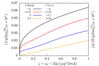
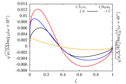
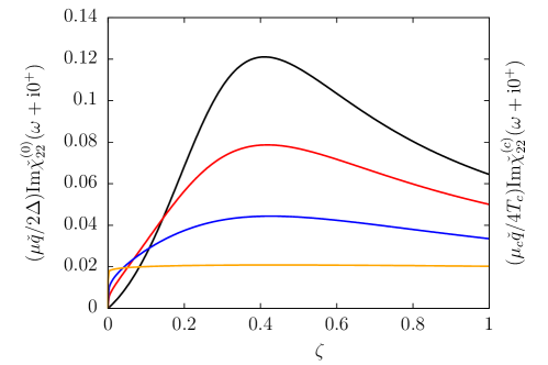
Figure 1: The order-parameter response functions (top left pannel: phase-phase, top right pannel: modulus-phase, bottom pannel: modulus-modulus response) are shown as functions of the reduced drive frequency $\zeta=(\omega-2\Delta)/(\mu{q}^{2}/2m\Delta)$ of Eq. (50) in the long wavelength limit after multiplication by the power of $q$ which ensures a finite non zero limit when $q\to 0$. Their value at zero temperature ($\chi^{(0)}_{ij}$) coincide up to a proportionality factor (shown in the $y$-axis labels) with their value near the phase transition ($\chi^{(c)}_{ij}$) at a slightly different interaction strength $1/k_{F}a$ obtain using the correspondence Eq. (59). The values of $1/k_{F}a$ used to span the BCS side of the crossover at $T=0$ correspond with the mean-field equation-of-state to $\mu/\Delta=+\infty$, $2$, $0.86$ and $0.07$ (respectively black, blue, red and orange lines). At $T\to T_{c}$ they correspond to $\mu_{c}/T_{c}=+\infty$, $4.2$, $1.8$ and $0.15$. For $\chi_{12}$, the BCS limit $\mu/\Delta,\mu_{c}/T_{c}\to+\infty$ is reached logarithmically such that we have used the finite values $\mu/\Delta=10$, $1/k_{F}a_{0}=-1.5$ at $T=0$ and $\mu_{c}/T_{c}=20.6$, $1/k_{F}a_{c}=-1.6$ near $T_{c}$.

V.3 Density matrix elements in the long wavelength limit

We now study the density responses of the system $\chi_{i3}$, $i=1,2,3$ in the long wavelength limit $q\to 0$ at energies above but close to $2\Delta$. In the long wavelength limit $q\to 0$ (at fixed $\zeta$), the three matrix elements needed to compute the density response functions are given by:

$$\delta\check{\Pi}_{13} \equiv \check{\Pi}_{13}+\check{\Pi}_{11}={\pi^{2}}\frac{\mu}{2\Delta}\mbox{tanh}\left(\frac{\Delta}{2T}\right)f_{13}(\zeta)\check{q}+O(q^{2})\qquad\mbox{with}\qquad f_{13}(\zeta)=\sqrt{1-\zeta}\$$ (63)

$$\delta\check{\Pi}_{23} \equiv \check{\Pi}_{23}+\check{\Pi}_{12}=\pi^{2}\left(\frac{\mu}{2\Delta}\right)^{3/2}\mbox{tanh}\left(\frac{\Delta}{2T}\right)\left[\zeta g_{12}\left(\frac{\mu}{T},\frac{\Delta}{T}\right)+g_{23}\left(\frac{\mu}{T},\frac{\Delta}{T}\right)\right]\check{q}^{2}+O(q^{3})$$ (64)

$$\delta\check{\Pi}_{33} \equiv \check{\Pi}_{33}+\check{\Pi}_{11}+2\check{\Pi}_{13}=g_{33}\left(\frac{\mu}{T},\frac{\Delta}{T}\right)\check{q}^{2}+\frac{\pi^{2}}{2}\frac{\mu^{2}}{4\Delta^{2}}\mbox{tanh}\left(\frac{\Delta}{2T}\right)f_{33}(\zeta)\check{q}^{3}+O(q^{4})$$ (65)

$$\mbox{with}\qquad f_{33} = {(\zeta-2)\sqrt{1-\zeta}-\zeta^{2}\mbox{ln}\frac{1+\sqrt{1-\zeta}}{\sqrt{\zeta}}-\frac{i\pi\zeta^{2}}{2}}$$ (66)

$$\pi^{2}\left(\frac{M}{2D}\right)^{3/2} \!\!\!\!\!\!\!\!\!\!\!\!\mbox{tanh}\left(\frac{D}{2}\right)g_{23}(M,D)=\frac{\pi}{3}\mathcal{P}\int_{-M/D}^{\infty}\frac{d\xi\sqrt{\xi+{M}/{D}}^{3}}{\xi\epsilon^{3}}\mbox{tanh}\frac{D\epsilon}{2}+\frac{\pi D}{6}\mathcal{P}\int_{-M/D}^{\infty}\frac{\xi d\xi\sqrt{\xi+{M}/{D}}^{3}}{\epsilon^{2}\mbox{cosh}^{2}\frac{D\epsilon}{2}}$$

$$\mbox{and}\!\!\!\!\qquad g_{33}(M,D)=\frac{\pi}{16}\mathcal{P}\int_{-M/D}^{\infty}\frac{d\xi\sqrt{\xi+{M}/{D}}}{\mbox{cosh}^{2}\frac{D\epsilon}{2}\epsilon^{5}}\left[-2D\epsilon\left(\xi\epsilon^{2}+\frac{2}{3}\left[1-2{\xi^{2}(1+\epsilon^{2})}\right]\left(\xi+{M}/{D}\right)\right)\right.$$

$$\qquad\qquad\qquad\left.+\frac{\mbox{sinh}\frac{3D\epsilon}{2}}{\mbox{cosh}\frac{D\epsilon}{2}}\left(\xi\epsilon^{2}+2\left(\xi+{M}/{D}\right)\right)+\mbox{tanh}\frac{D\epsilon}{2}\left(\xi\epsilon^{2}+2\left(\xi+{M}/{D}\right)\left(1+\frac{2}{3}D^{2}\xi^{2}\epsilon^{2}\right)\right)\right].$$

Those expressions, like those of the modulus and phase matrix elements (51–53) are obtained by treating separately the resonant wavevectors (for the resonance condition $z=\epsilon_{\mathbf{k}+\mathbf{q}/2}+\epsilon_{\mathbf{k}-\mathbf{q}/2}$), located in this limit around the minimum $k_{0}$ of the BCS branch. For those wavevectors, we set

$$k=k_{0}+Kq,$$ (69)

and expand the integrand in (37) at fixed $K$. This yields the leading order contribution to $\Pi_{11}$, $\Pi_{22}$ and $\delta\Pi_{13}$. For $\Pi_{12}$, $\delta\Pi_{23}$ and $\delta\Pi_{33}$ the leading order is dominated by the wavevectors away from $k_{0}$ and is obtained by expanding directly in powers of $q$ at fixed $k$ (with a contribution of the quasiparticle-quasihole integrals from Eq. (38)). For $\delta\Pi_{33}$ specifically, the subleading order $O(q^{3})$ (which matters for the imaginary part of the response function $\textrm{Im}\,\chi_{33}$), is obtained by subtracting the leading one and then using the reparametrisation of the wavevectors, Eq. (69).

Using the expansions Eqs. (63–65), we obtain the expressions of the density response functions:

$$\chi_{13} = 1+\frac{\mu}{2\Delta}\frac{(\zeta g_{12}+g_{23})g_{12}-f_{13}f_{22}}{f_{11}f_{22}+g_{12}^{2}}\check{q}^{2}+O(q^{3})$$ (70)

$$\chi_{23} = -\sqrt{\frac{\mu}{2\Delta}}\frac{f_{13}g_{12}+(\zeta g_{12}+g_{23})f_{11}}{f_{11}f_{22}+g_{12}^{2}}\check{q}+O(q^{2})$$ (71)

$$\chi_{33} = g_{33}\check{q}^{2}+\pi^{2}\frac{\mu^{2}}{4\Delta^{2}}\mbox{tanh}\left(\frac{\Delta}{2T}\right)\left[\frac{f_{33}}{2}-\frac{2f_{13}(\zeta g_{12}+g_{23})g_{12}-f_{13}^{2}f_{22}+(\zeta g_{12}+g_{23})^{2}f_{11}}{f_{11}f_{22}+g_{12}^{2}}\right]\check{q}^{3}+O(q^{4}),$$ (72)

where we omit the evaluation of the functions $f_{ij}$ and $g_{ij}$ respectively in $\zeta$ and $(\mu/T,\Delta/T)$. The limiting behaviour near the phase transition follows immediately by using the limiting behaviour of $\Delta$ and $\mu$ from Eqs. (56–57) and replacing $g_{12}(\mu/T,\Delta/T)$ and $g_{23}(\mu/T,\Delta/T)$ by their finite nonzero limit $g_{12,c}(\mu/T_{c})$ and $g_{23,c}(\mu/T_{c})$ with

$$g_{23,c}(M)=\frac{2\sqrt{2}}{3\pi M^{3/2}}\int_{-M}^{+\infty}\frac{de(e+M)^{3/2}}{e\mbox{cosh}^{2}(e/2)}.$$ (73)

The function $g_{33}$, which gives only a $\zeta$-independent shift of $\mbox{Re}\,\chi_{33}$, diverges asymptotically as $O(\Delta/T_{c})^{-3/2}$ near the phase transition.

In Fig. 2, we show the density response functions on the BCS side of the crossover. Unlike for the order-parameter response functions, no exact correspondance between zero temperature and the transition temperature can be found by changing the interaction strength (this is due to the temperature dependence of $g_{23}$), so we show separately the functions at $T=0$ (in solid curves) and at $T\to T_{c}$ (in dashed curves). The difference between the $T=0$ and $T\to T_{c}$ curves (after the appropriate rescaling) remains however fairly small, and tends to 0 in the BCS limit (black curves). Remarkably, a minimum characteristic of the Popov-Andrianov collective mode is visible in all three density responses. In $\chi_{23}$, this minimum is a global minimum (for $\zeta\in[0,1]$) which exist (as in $\chi_{22}$ and $\chi_{12}$) from the BCS limit up until unitarity. For the density-density and density-phase responses $\chi_{33}$ and $\chi_{13}$, this minimum is a local minimum, which exists close to unitarity (blue curves) around $\zeta=0.1$. Because of the decoupling between the phase-density fluctuations and the modulus fluctuations in the weak-coupling limit, this minimum disappears from $\chi_{13}$ and $\chi_{33}$ in the weak-coupling limit $1/k_{F}a\to-\infty$ (black curves). After unitary, when approaching the BEC regime (orange curves), the resonances in all three density responses are replaced by a sharp edge in $\omega\to 2\Delta^{+}$ ($\zeta\to 0^{+}$). This is the same phenomenon as in the order-parameter response functions.

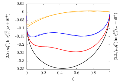
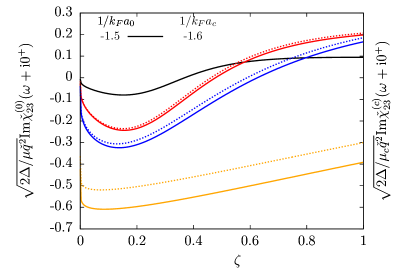
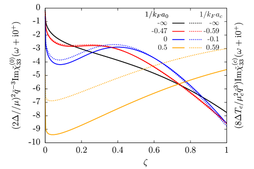
Figure 2: The density response functions (top left pannel: density-phase, top right pannel: density-modulus, bottom pannel: density-density response) are shown as functions of the reduced drive frequency $\zeta=(\omega-2\Delta)/(\mu{q}^{2}/2m\Delta)$ of Eq. (50) in the long wavelength limit after multiplication by the power of $q$ which ensures a finite non zero limit when $q\to 0$. Their values at zero temperature ($\chi^{(0)}_{ij}$, solid lines) are compared to their value near the phase transition ($\chi^{(c)}_{ij}$, dashed lines) after the appropriate rescaling and the change of interaction strength which brings the order-parameter responses on the same line (see Fig. 1, and the correspondence Eq. (59)). Please refer to the caption of Fig. 1 for the values of $\mu/\Delta$ and of $\mu_{c}/T_{c}$ corresponding to the chosen values of $1/k_{F}a$.

V.4 Coexistence with the phononic collective modes near $T_{c}$

To compare the Popov-Andrianov resonance to the other collective effects of a superfluid Fermi gases near $T_{c}$, we show in Fig. 3 the response functions from $\omega=0$ up until $\omega>3\Delta$ in the strong coupling regime and temperature close to $T_{c}$. The sharpest feature in both the order-parameter and density responses is the resonance, at very low energy (that is at $\omega=uq$ with a velocity $u\propto\sqrt{T_{c}-T}$), of the collisionless phononic collective mode found in Klimin et al. (2019). Still at phononic energies $\omega\propto q$, the density-density response function shows a broad peak caused entirely by $\Pi_{33}$ (shown as a black dashed line) and also noticed in Klimin et al. (2019). This peak exists also in the normal phase and may be interpreted as the zero sound of an ideal Fermi gas. Finally, inside the first window $[2\Delta,\omega_{2}]$ of analyticity of the pair-breaking continuum, all response functions show the peak characteristic of the Popov-Andrianov resonance, whose shape matches the one shown on Figs. 1 and 2. Due to the absence of rescaling with the wavevector $q$ in Fig. 3, the peak is much more intense in the modulus-modulus response, and to a lesser extent in the modulus-density response, than in the density-density response.

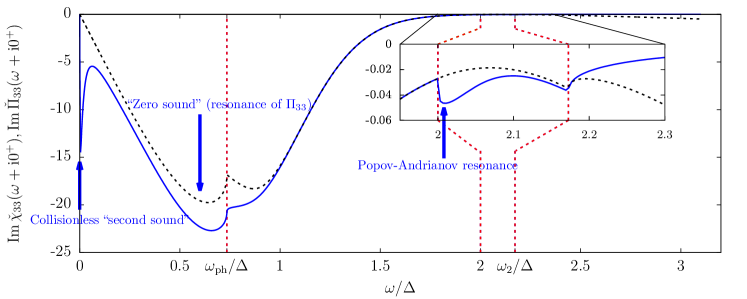
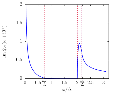
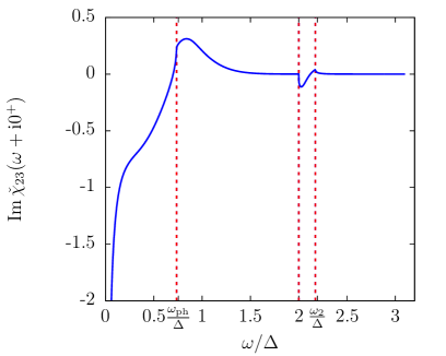
Figure 3: The density-density (top pannel), modulus-modulus (bottom left pannel) and modulus-density (bottom right pannel) response functions shown in function of the drive frequency $\omega$. The curves were drawn in the strong coupling regime ($1/k_{\rm F}a\simeq-0.1$, $\mu_{c}/T_{c}\simeq 1.8$), near the transition temperature ($\Delta/T=0.1$) and at long wavelength ($\check{q}=0.1$). The dimensionless response functions are shown this time without rescaling and from $\omega=0$ until far inside the pair-breaking continuum. The vertical dashed lines show the angular points of the fermionic continua, from left to right $\omega_{\rm ph}$, $\omega_{1}$($=2\Delta$) and $\omega_{2}$. On the top panel, the black dashed line is the pure density contribution $\mbox{Im}\ \Pi_{33}$ to the density-density response (see Eq. (46)) and the inset is a zoom on the behaviour near $\omega=2\Delta$.

V.5 Experimental protocol

Our results suggest a very simple experimental protocol to observe the resonance: using a Bragg spectroscopic measurement as in Ref. Hoinka et al. (2017), one should observe that the first extremum above $2\Delta$ varies quadratically (both in location and width) with $q$, a behavior which can be viewed as the fingerprint of the Popov-Andrianov-Higgs mode. The optimal interaction regime is around unitarity and the optimal wavevector is around $0.5\times\sqrt{2m\Delta}$ ($q$ should not be too small to avoid the $q^{3}$ cancellation of $\chi_{33}$ near $2\Delta$ but not too large either otherwise the minimum is reabsorbed by the continuum edge, see the lower panels of Fig. 5).

Alternatively, the resonance could be observed through the modulus-density response function $\chi_{23}$ by $(i)$ exciting the order-parameter modulus $\delta|\Delta|$ through a modulation of the scattering length at frequency $\omega$ and wavelength $2\pi/q$ and $(ii)$ measuring the intensity of the density modulation $\delta\rho$ at wavelength $2\pi/q$. This should be easier than the scheme of Ref. Kurkjian et al. (2019) which proposed to measure $\chi_{22}$ by interferometry. Using the symmetry of the response matrix $\chi$, one can also excite the density $\delta\rho$ (by a Bragg pulse Hoinka et al. (2017) or using the trapping potential Patel et al. (2019)) and measure the order-parameter modulus $\delta|\Delta|$ either by interferometry or by bosonizing the Cooper pairs through a fast sweep of the scattering length, as was done in Behrle et al. (2018).

VI At shorter wavelengths

Outside the long wavelength limit, that is $q\approx\sqrt{2m\Delta},\sqrt{2m\mu}$ when $\mu$ and $\Delta$ are comparable, we study the response functions by performing numerically the integral over internal wavevectors $\mathbf{k}$ in Eqs. (38) and (37) (see Appendix B for more details on the numerical implementation).

VI.1 At zero temperature

VI.1.1 Weak-coupling regime

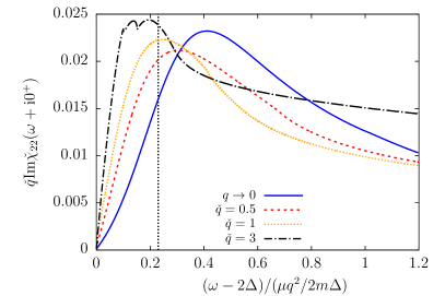
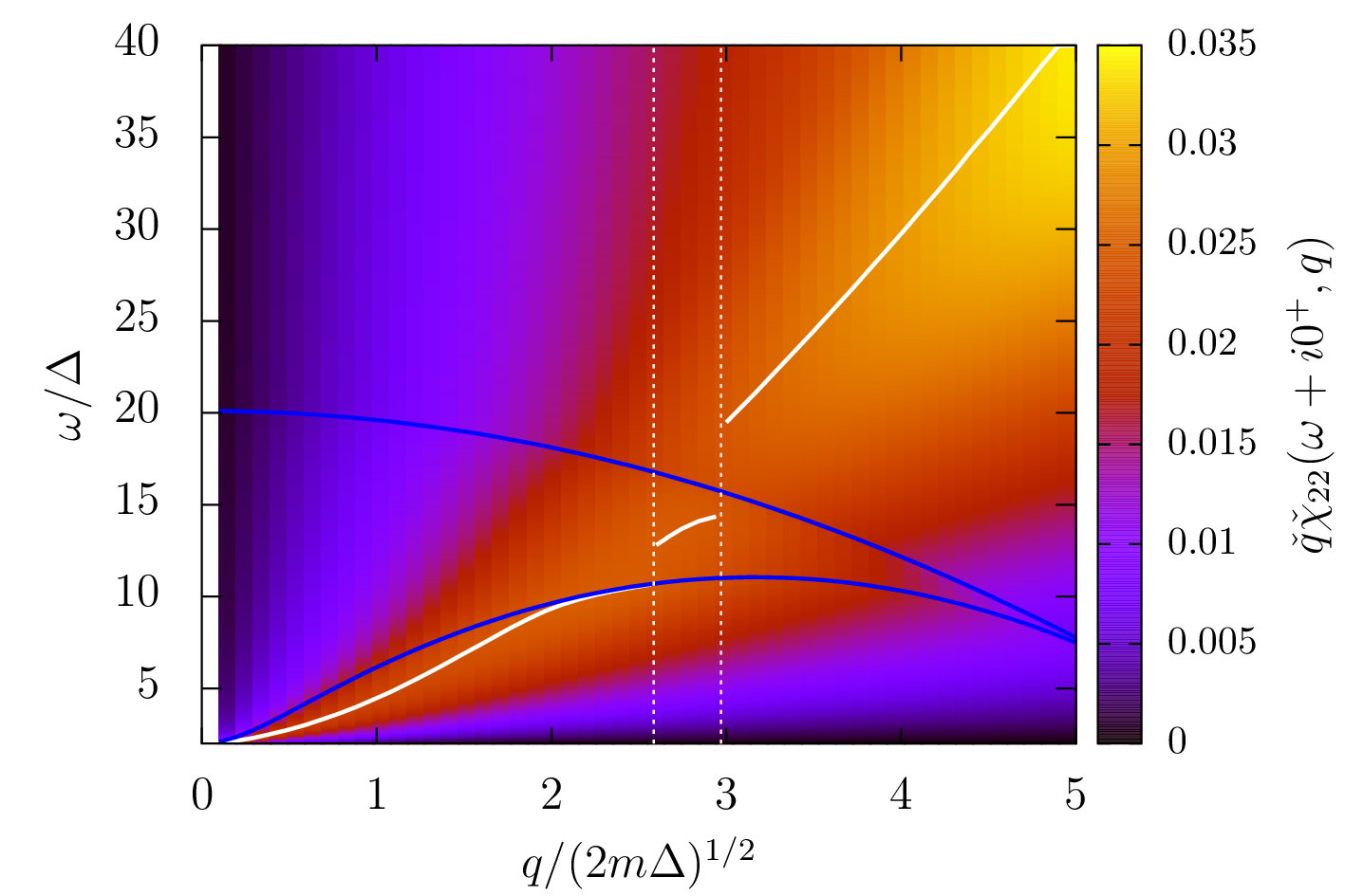
Figure 4: Left panel: the modulus-modulus response function is shown as a function of $(\omega-2\Delta)/(\mu{q}^{2}/2m\Delta)$ at weak-coupling $\mu/\Delta=10$. The wavevector $q$ varies from $q\to 0$ (solid blue line, see section V), $\check{q}=0.5$ (red dashed line), $\check{q}=1$ (orange dotted line) to $\check{q}=3$ (black dash-dotted line), and the response function is multiplied by $\check{q}$. The vertical dotted line indicates the reduced eigenergy $\mbox{Re}\zeta_{s}\simeq 0.23$ of the pole found (when $q\to 0$) in the analytic continuation (see Eq. 55) through $[2\Delta,\omega_{2}]$. Right panel: the same evolution is shown in colors as functions of both the wavevector $q$ on the $x$-axis and drive frequency $\omega$ on the $y$-axis. The response function is still multiplied by $\check{q}$. Superimposed to the color plot, the angular points $\omega_{2}$ (lower blue solid line) and $\omega_{3}$ (upper blue solid line), and the location of the global maximum of the function $\omega\mapsto\chi_{22}$ (white solid line). As $q$ increases, this maximum jumps from the interval $[2\Delta,\omega_{2}]$ where it is located at low $q$, to $[\omega_{2},\omega_{3}]$ and eventually to $[\omega_{3},+\infty[$ at large $q$. Each jump is marked by a vertical white dotted line.

On the left panel of Fig. 4, we show the modulus-modulus response at relatively weak-coupling ($\mu/\Delta=10$) and zero temperature as a function of $\omega$ (rescaled as in the long wavelength section) for increasing values of the wavevector $q$. On the right panel, we show the same dispersion relation but in colors, with $q$ on the $x$-axis and $\omega$ on the $y$-axis. The Popov-Andrianov resonance we have characterized at low $q$ remains as a broader and shallower maximum as $q$ increases (see the rescaling of the $x$ and $y$-axis on the left panel of Fig. 4) that travels roughly quadratically through the continuum. In the modulus-modulus response function, the augmentation of wavevector is thus unfavourable for the observation of the resonance in the pair-breaking continuum. Note that the location of the maximum is discontinuous when crossing $\omega_{2}$ and $\omega_{3}$ (which both decrease with $q$), but remains a monotonously increasing function of $q$. The non-monotonic behavior of the collective mode eigenfrequency $z_{q}$ found in the analytic continuation through the interval $[2\Delta,\omega_{2}]$ of the real axis Kurkjian et al. (2019) is thus not reflected on the response function. In fact the angular points $\omega_{2}$ and $\omega_{3}$ only slightly affect the shape of the resonance when they cross it (see in particular the black curve on the left panel of Fig. 4). This is consistent with the finding of Ref. Castin and Kurkjian (2019) (see in particular section 4.8 therein): at large $q$, the analytic continuations through windows $[\omega_{2},\omega_{3}]$ and $[\omega_{3},+\infty[$ predict a pole with an eigenfrequency close to that of the Popov-Andrianov branch in window $[2\Delta,\omega_{2}]$. The same robustness towards the choice of the real axis interval through which the analytic continuation is made was noticed by Ref. Klimin et al. (2019) for the phononic modes. It is a sign that the Popov-Andrianov collective mode is a fundamental physical phenomenon, which does not depend on a specific configuration of the fermionic continuum.

VI.1.2 Strong-coupling regime

Conversely, the increase of $q$ favours the observability of the resonance in both the modulus-density and density-density response functions at strong coupling. On Fig. 5, we show $\chi_{23}$ and $\chi_{33}$ (as well as $\chi_{22}$) at unitarity ($\mu/\Delta\simeq 0.86$) and still at zero temperature. As long as it does not encounter the singularity in $\omega_{3}$, a smooth extremum (in $\chi_{23}$ and $\chi_{33}$ it’s a minimum) whose location increases quadratically with $q$ remains visible. The resonance broadens with $q$, but this is compensated by a deepening of the resonance peak roughly as $q$ in $\chi_{23}$ and as $q^{3}$ in $\chi_{33}$. The resonance in $\chi_{33}$ is caused by the order-parameter contribution $\chi_{33}-\Pi_{33}$ to the density-density fluctuations (compare the blue dotted and the blue solid line on the bottom left panel of Fig. 5), in which it is a global minimum as a function of $\omega$ (rather than a local minimum in $\chi_{33}$). To emphasize the dispersion of the resonance, we thus plot on the bottom right panel of Fig. 5, $\Pi_{33}-\chi_{33}$ divided by $q^{3}$ in colors as a function of $\omega$ and $q$. The global extremum of $\omega\mapsto\Pi_{33}-\chi_{33}$ is shown as a function of $q$ in white solid line. As long as it stays in the window $[2\Delta,\omega_{2}]$, it varies approximatively quadratically with $q$.

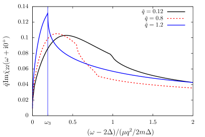
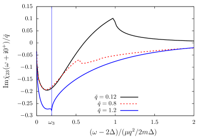
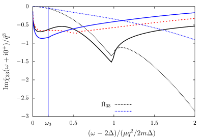
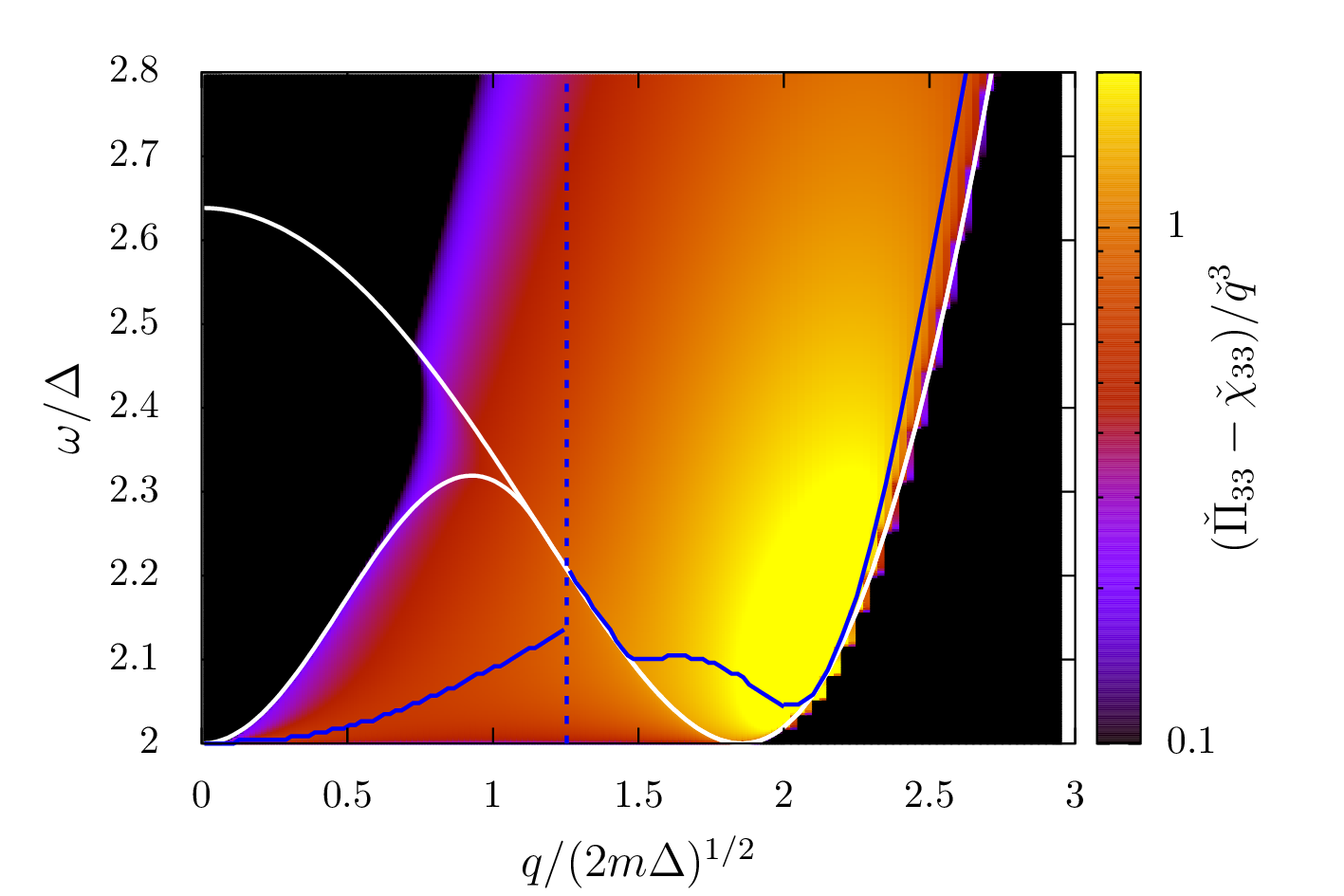
Figure 5: The modulus-modulus (top left panel), modulus-density (top right panel) and density-density (bottom left panel) response functions are shown at unitarity ($\mu/\Delta\simeq 0.86$) in function of the reduced drive frequency $(\omega-2\Delta)/(\mu{q}^{2}/2m\Delta)$ for increasing value of the wavevector $q/\sqrt{2m\Delta}=0.12$ (black solid line), $0.8$ (red dashed line) and $1.2$ (blue solid line). For $q/\sqrt{2m\Delta}=1.2$, we show by a vertical blue line the value of the singularity $\omega_{2}=\omega_{3}\simeq 2.23\Delta$ where the shape of the response functions changes dramatically. In the bottom left panel, we also show the contribution of the pure density-density fluctuations $\Pi_{33}$ to the total density response (black and blue dotted line). Bottom right panel: $\check{\Pi}_{33}-\check{\chi}_{33}$ is shown in colors as a function of $\omega$ and $q$ (the color scale is logarithmic) after division by $\check{q}^{3}$. The angular points $\omega_{2}$ and $\omega_{3}\geq\omega_{2}$ are superimposed on the color plot as white solid lines. The global extremum of the function $\omega\mapsto\chi_{33}(\omega+i0^{+})-\Pi_{33}(\omega+i0^{+})$ is shown as a blue solid line. Its location is discontinuous in $\check{q}\simeq 1.25$ (vertical dashed line) after which it coincides with the angular point $\omega_{3}$ for a range of values of $q$.

Contrarily to what happens at weak-coupling, the resonance shape at strong coupling is much distorted when going through the singularity $\omega_{3}$. This effect is particularly visible on the modulus-modulus and modulus-density responses (upper panels of Fig. 5) where the resonance seems broken in $\omega_{3}$ such that the smooth extremum has disappeared in favour of a sharp extremum in $\omega_{3}$. On the color plot of Fig. 5, the quadratic growth of the resonance frequency is also visibly halted when it encounters the angular point in $\omega_{3}$. This is not surprising since the poles found in the analytic continuation through windows $[2\Delta,\omega_{3}]$ and $[\omega_{3},+\infty[$ are very far apart in this regime Castin and Kurkjian (2019). For the value $q/\sqrt{2m\Delta}=1.2$ used in Fig. 5, the analytic continuation through the interval $[2\Delta,\omega_{3}]$ has a pole in $z_{q}/\Delta=1.93-0.41i$. In the interval $[\omega_{3},+\infty[$, the pole is in $z_{q}/\Delta=0.86-0.020i$, with a much lower value of the eigenfrequency and a small damping rate which give this “upper tail” appearance to the response functions at $\omega>\omega_{3}$. Above $\omega_{3}$, the behavior of the response functions is in fact similar to what happens in the BEC regime (see below Sec. VI.1.3), with a sharp edge pinned at $\omega_{3}$ (which becomes the lower edge of the continuum when $q=2\sqrt{2m\mu}$).

VI.1.3 In the BEC regime

In the BEC regime (that is for us when $\mu<0$), the lower-edge of the pair-breaking continuum is no longer flat at low $q$, but increases quadratically with $q$. Although a pole can be found in the analytic continuation through the interval $[\omega_{3},\infty[$ (the only one available when $\mu<0$), its real part always stays below $\omega_{3}$, such that no smooth peak appears in the response function. Instead there is only a sharp feature pinned at the lower-edge of the continuum. Fig. 6, shows the example of the modulus-modulus response function (the other responses have a similar behavior) at $\mu/\Delta=-1$ ($1/k_{F}a\simeq 1.3$). This sharp feature can hardly be interpreted as a collective mode and only reflects the incoherent response of the fermionic continuum when the pairs are tightly bound.

Figure 6: The modulus-modulus response function $\chi_{22}$ in the BEC regime ($\mu/\Delta=-1$, $1/k_{\rm F}a\simeq 1.3$) is shown in colors as a function of the wavevector $q$ and drive frequency $\omega$. The lower edge $\omega_{3}=2\sqrt{(\hbar^{2}q^{2}/8m+|\mu|)^{2}+\Delta^{2}}$ is shown as a white solid line.

VI.2 Near $T_{c}$

At nonzero temperature and even near $T_{c}$, we have shown in section V that the Popov-Andrianov resonance exists in the limit $q\to 0$ and is almost insensitive to the quasiparticle-quasihole contributions (38) to the fluctuation matrix $\Pi$. This is no longer the case at higher $q$. The angular point $\omega_{\rm ph}$ of the quasiparticle-quasihole continuum in particular destroys the resonance as it increases (initially linearly) with $q$. This effect is illustrated on Fig. 7 showing the modulus-modulus response function near $T_{c}$: at $q\sqrt{2\Delta/m}=0.12$ (orange dashed curve on Fig. 7) the lower tail of the resonance is trimmed by the angular point at $\omega_{\rm ph}$, and at $q\sqrt{2\Delta/m}=0.3$ (long-dashed green curve) it is completely hidden. This can be understood by a simple reasoning: near $T_{c}$, $\omega_{\rm ph}$ varies as $q\sqrt{2\mu/m}$ at low $q$ Klimin et al. (2019), such that it reaches $2\Delta$ for $\check{q}=q/\sqrt{2m\Delta}\approx\sqrt{\Delta/\mu}=O(T_{c}-T)^{1/4}$. The long wavelength limit near $T_{c}$ is thus limited to $q^{2}/2m\ll\Delta^{2}/\mu$ (as in the weak-coupling case at $T=0$ see Eq. (90) in Castin and Kurkjian (2019)).

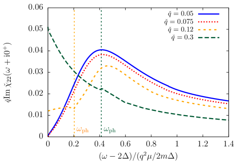
Figure 7: The dispersion of the Popov-Andrianov branch in the modulus-modulus response function near the transition temperature ($\Delta/T=0.1$) and in the weak-coupling regime $\mu_{c}/T_{\rm c}\simeq\mu/T=10$ ($1/k_{\rm F}a\simeq-1.15$ with the mean-field equation-of-state). The modulus-modulus response function is plotted as a function of the reduced drive frequency $(\omega-2\Delta)/({q}^{2}\mu/2m\Delta)$ for the values of the wavector $q/\sqrt{2m\Delta}=0.05,\ 0.075,\ 0.12$ and $0.3$ (respectively solid blue, dotted red, dashed orange and long-dashed green lines). The resonance is well visible at low-$q$ but it disappears as the angular point of the quasiparticle-quasihole continuum $\omega_{\rm ph}$ (shown by a vertical dotted line at $(\omega-2\Delta)/({q}^{2}\mu/2m\Delta)=0.204$ and $0.413$ for respectively $q/\sqrt{2m\Delta}=0.12$ and $0.3$) rises with $q$.

VII Conclusion

We have computed the response function matrix of a superfluid Fermi gas in the Random Phase Approximation at nonzero temperature, and used it to study the observability of the order-parameter collective modes. We have shown that the appearance of a resonance inside the pair-breaking continuum associated to the Popov-Andrianov-“Higgs” mode is a very robust phenomenon which concerns not only the modulus-modulus response function but also the modulus-density and density-density responses, which are easier to measure. At weak-coupling the resonance is observable at all values of the wavevector $q$ and is only weakly sensitive to the angular points created in the response functions by the changes of structure of the fermionic continuum. At nonzero temperature, we have shown analytically that the resonance is not destroyed by the presence of excited fermionic quasiparticles, and retains approximatively the same shape as when $T=0$. It also coexists with the low-velocity phononic collective mode which RPA predicts near $T_{c}$. The spectral weight of the resonance is enhanced in the modulus-density and density-density responses when $T$ increases, which should favour its observability.

Appendix A Derivation of the equations of motion

We give here a few additional steps leading to the equations of motion (22–25). In the particle basis, the equations of motion take the form:

$$\!\!\!\!\!\!\!\!\!\!\!\!{i}\hbar\frac{{d}\hat{d}_{\mathbf{k}}^{\mathbf{q}}}{{d}t} \!\!= \!\!\!\xi^{+}_{\mathbf{k}\mathbf{q}}\hat{d}_{\mathbf{k}}^{\mathbf{q}}-\Delta_{0}(\hat{n}_{\mathbf{k}}^{\mathbf{q}}+\hat{\bar{n}}_{\mathbf{k}}^{\mathbf{q}})+z_{\mathbf{k}\mathbf{q}}^{+}(\hat{\Delta}^{\mathbf{q}}+\phi(\mathbf{q}))+d_{\mathbf{k}\mathbf{q}}^{+}\frac{g_{0}\hat{n}^{\mathbf{q}}_{\uparrow}+g_{0}\hat{n}^{\mathbf{q}}_{\downarrow}+u_{+}(\mathbf{q})}{2}-d_{\mathbf{k}\mathbf{q}}^{-}\frac{g_{0}\hat{n}^{\mathbf{q}}_{\uparrow}-g_{0}\hat{n}^{\mathbf{q}}_{\downarrow}-u_{-}(\mathbf{q})}{2}$$ (74)

$$\!\!\!\!\!\!\!\!\!\!\!\!{i}\hbar\frac{{d}\hat{\bar{d}}_{\mathbf{k}}^{\mathbf{q}}}{{d}t} \!\!= \!\!\!-\xi^{+}_{\mathbf{k}\mathbf{q}}\hat{\bar{d}}_{\mathbf{k}}^{\mathbf{q}}+\Delta_{0}(\hat{n}_{\mathbf{k}}^{\mathbf{q}}+\hat{\bar{n}}_{\mathbf{k}}^{\mathbf{q}})-z_{\mathbf{k}\mathbf{q}}^{+}(\hat{\bar{\Delta}}^{\mathbf{q}}+\bar{\phi}(\mathbf{q}))-d_{\mathbf{k}\mathbf{q}}^{+}\frac{g_{0}\hat{n}^{\mathbf{q}}_{\uparrow}+g_{0}\hat{n}^{\mathbf{q}}_{\downarrow}+u_{+}(\mathbf{q})}{2}-d_{\mathbf{k}\mathbf{q}}^{-}\frac{g_{0}\hat{n}^{\mathbf{q}}_{\uparrow}-g_{0}\hat{n}^{\mathbf{q}}_{\downarrow}-u_{-}(\mathbf{q})}{2}$$ (75)

$$\!\!\!\!\!\!\!\!\!\!\!\!{i}\hbar\frac{{d}\hat{n}_{\mathbf{k}}^{\mathbf{q}}}{{d}t} \!\!= \!\!\!-\xi^{-}_{\mathbf{k}\mathbf{q}}\hat{n}_{\mathbf{k}}^{\mathbf{q}}-\Delta_{0}(\hat{d}_{\mathbf{k}}^{\mathbf{q}}-\hat{\bar{d}}_{\mathbf{k}}^{\mathbf{q}})-z_{\mathbf{k}\mathbf{q}}^{-}(g_{0}\hat{n}^{\mathbf{q}}_{\downarrow}+u_{\uparrow}(\mathbf{q}))+d_{\mathbf{k}\mathbf{q}}^{-}\frac{\hat{\Delta}^{\mathbf{q}}+\hat{\bar{\Delta}}^{\mathbf{q}}+\phi_{+}(\mathbf{q})}{2}+d_{\mathbf{k}\mathbf{q}}^{+}\frac{\hat{\Delta}^{\mathbf{q}}-\hat{\bar{\Delta}}^{\mathbf{q}}+\phi_{-}(\mathbf{q})}{2}$$ (76)

$$\!\!\!\!\!\!\!\!\!\!\!\!{i}\hbar\frac{{d}\hat{\bar{n}}_{\mathbf{k}}^{\mathbf{q}}}{{d}t} \!\!= \!\!\!\xi^{-}_{\mathbf{k}\mathbf{q}}\hat{\bar{n}}_{\mathbf{k}}^{\mathbf{q}}-\Delta_{0}(\hat{d}_{\mathbf{k}}^{\mathbf{q}}-\hat{\bar{d}}_{\mathbf{k}}^{\mathbf{q}})+z_{\mathbf{k}\mathbf{q}}^{-}(g_{0}\hat{n}^{\mathbf{q}}_{\uparrow}+u_{\downarrow}(\mathbf{q}))-d_{\mathbf{k}\mathbf{q}}^{-}\frac{\hat{\Delta}^{\mathbf{q}}+\hat{\bar{\Delta}}^{\mathbf{q}}+\phi_{+}(\mathbf{q})}{2}+d_{\mathbf{k}\mathbf{q}}^{+}\frac{\hat{\Delta}^{\mathbf{q}}-\hat{\bar{\Delta}}^{\mathbf{q}}+\phi_{-}(\mathbf{q})}{2},$$ (77)

where we generalize the notations of Refs. Anderson (1958); Kurkjian (2016) to nonzero temperature:

$$z_{\mathbf{k}\mathbf{q}}^{\pm}(T) = \left(\frac{1}{2}-\langle\hat{n}_{\mathbf{k}_{+}}^{\mathbf{0}}\rangle_{T}\right)\pm\left(\frac{1}{2}-\langle\hat{n}_{\mathbf{k}_{-}}^{\mathbf{0}}\rangle_{T}\right)=\frac{U_{\mathbf{k}_{+}}^{2}-V_{\mathbf{k}_{+}}^{2}}{2}(1-2f_{\mathbf{k}_{+}})\pm\frac{U_{\mathbf{k}_{-}}^{2}-V_{\mathbf{k}_{-}}^{2}}{2}(1-2f_{\mathbf{k}_{-}})$$ (78)

$$= \left[\frac{\xi_{\mathbf{k}_{+}}}{2\epsilon_{\mathbf{k}_{+}}}\pm\frac{\xi_{\mathbf{k}_{-}}}{2\epsilon_{\mathbf{k}_{-}}}\right](1-f_{\mathbf{k}_{+}}-f_{\mathbf{k}_{-}})-\left[\frac{\xi_{\mathbf{k}_{+}}}{2\epsilon_{\mathbf{k}_{+}}}\mp\frac{\xi_{\mathbf{k}_{-}}}{2\epsilon_{\mathbf{k}_{-}}}\right](f_{\mathbf{k}_{+}}-f_{\mathbf{k}_{-}})$$

$$d_{\mathbf{k}\mathbf{q}}^{\pm}(T) = \langle\hat{d}_{\mathbf{k}+\mathbf{q}/2}^{\mathbf{0}}\rangle_{T}\pm\langle\hat{d}_{\mathbf{k}-\mathbf{q}/2}^{\mathbf{0}}\rangle_{T}=-\left[U_{\mathbf{k}_{+}}V_{\mathbf{k}_{+}}(1-2f_{\mathbf{k}_{+}})\pm U_{\mathbf{k}_{-}}V_{\mathbf{k}_{-}}(1-2f_{\mathbf{k}_{-}})\right]$$ (79)

$$= -\left[\frac{\Delta}{2\epsilon_{\mathbf{k}_{+}}}\pm\frac{\Delta}{2\epsilon_{\mathbf{k}_{-}}}\right](1-f_{\mathbf{k}_{+}}-f_{\mathbf{k}_{-}})+\left[\frac{\Delta}{2\epsilon_{\mathbf{k}_{+}}}\mp\frac{\Delta}{2\epsilon_{\mathbf{k}_{-}}}\right](f_{\mathbf{k}_{+}}-f_{\mathbf{k}_{-}}).$$

Adding and subtracting Eq. (74) to (75) and Eq. (76) to (77) and performing the change of basis (21) (one can use the explicit relations given in Appendix C of Kurkjian (2016)) yields the equations of motion (22–25) in the quasiparticle basis. Rederiving with respect to time yields:

$$-(\epsilon_{\mathbf{k}\mathbf{q}}^{+})^{2}\hat{y}_{\mathbf{k}}^{\mathbf{q}}-\frac{{d}^{2}\hat{y}_{\mathbf{k}}^{\mathbf{q}}}{{d}t^{2}} = (1-f_{\mathbf{k}_{+}}-f_{\mathbf{k}_{-}})\left[W_{\mathbf{k}\mathbf{q}}^{-}{i}\hbar\partial_{t}\left(\delta\hat{\Delta}^{\mathbf{q}}+\delta\hat{\bar{\Delta}}^{\mathbf{q}}+\phi_{+}(\mathbf{q})\right)-w_{\mathbf{k}\mathbf{q}}^{+}{i}\hbar\partial_{t}\left(g_{0}\left[\delta\hat{n}_{\uparrow}^{\mathbf{q}}+\delta\hat{{n}}_{\downarrow}^{\mathbf{q}}\right]+u_{+}(\mathbf{q})\right)\right.$$ (80)

$$\left.+\epsilon_{\mathbf{k}\mathbf{q}}^{+}W_{\mathbf{k}\mathbf{q}}^{+}\left(\hat{\Delta}^{\mathbf{q}}-\hat{\bar{\Delta}}^{\mathbf{q}}+\phi_{-}(\mathbf{q})\right)-\epsilon_{\mathbf{k}\mathbf{q}}^{+}w_{\mathbf{k}\mathbf{q}}^{-}\left(g_{0}\left[\hat{n}_{\uparrow}^{\mathbf{q}}-\hat{{n}}_{\downarrow}^{\mathbf{q}}\right]-u_{-}(\mathbf{q})\right)\right]$$

$$-(\epsilon_{\mathbf{k}\mathbf{q}}^{-})^{2}\hat{h}_{\mathbf{k}}^{\mathbf{q}}-\frac{{d}^{2}\hat{h}_{\mathbf{k}}^{\mathbf{q}}}{{d}t^{2}} = (f_{\mathbf{k}_{+}}-f_{\mathbf{k}_{-}})\left[w_{\mathbf{k}\mathbf{q}}^{+}{i}\hbar\partial_{t}\left(\delta\hat{\Delta}^{\mathbf{q}}+\delta\hat{\bar{\Delta}}^{\mathbf{q}}+\phi_{+}(\mathbf{q})\right)+W_{\mathbf{k}\mathbf{q}}^{-}{i}\hbar\partial_{t}\left(g_{0}\left[\delta\hat{n}_{\uparrow}^{\mathbf{q}}+\delta\hat{{n}}_{\downarrow}^{\mathbf{q}}\right]+u_{+}(\mathbf{q})\right)\right.$$ (81)

$$\left.+\epsilon_{\mathbf{k}\mathbf{q}}^{-}w_{\mathbf{k}\mathbf{q}}^{-}\left(\hat{\Delta}^{\mathbf{q}}-\hat{\bar{\Delta}}^{\mathbf{q}}+\phi_{-}(\mathbf{q})\right)+\epsilon_{\mathbf{k}\mathbf{q}}^{-}W_{\mathbf{k}\mathbf{q}}^{+}\left(g_{0}\left[\hat{n}_{\uparrow}^{\mathbf{q}}-\hat{{n}}_{\downarrow}^{\mathbf{q}}\right]-u_{-}(\mathbf{q})\right)\right]$$

$$-(\epsilon_{\mathbf{k}\mathbf{q}}^{+})^{2}\hat{s}_{\mathbf{k}}^{\mathbf{q}}-\frac{{d}^{2}\hat{s}_{\mathbf{k}}^{\mathbf{q}}}{{d}t^{2}} = (1-f_{\mathbf{k}_{+}}-f_{\mathbf{k}_{-}})\left[W_{\mathbf{k}\mathbf{q}}^{+}{i}\hbar\partial_{t}\left(\hat{\Delta}^{\mathbf{q}}-\hat{\bar{\Delta}}^{\mathbf{q}}+\phi_{-}(\mathbf{q})\right)-w_{\mathbf{k}\mathbf{q}}^{-}{i}\hbar\partial_{t}\left(g_{0}\left[\hat{n}_{\uparrow}^{\mathbf{q}}-\hat{{n}}_{\downarrow}^{\mathbf{q}}\right]-u_{-}(\mathbf{q})\right)\right.$$ (82)

$$\left.+\epsilon_{\mathbf{k}\mathbf{q}}^{+}W_{\mathbf{k}\mathbf{q}}^{-}\left(\delta\hat{\Delta}^{\mathbf{q}}+\delta\hat{\bar{\Delta}}^{\mathbf{q}}+\phi_{+}(\mathbf{q})\right)-\epsilon_{\mathbf{k}\mathbf{q}}^{+}w_{\mathbf{k}\mathbf{q}}^{+}\left(g_{0}\left[\delta\hat{n}_{\uparrow}^{\mathbf{q}}+\delta\hat{{n}}_{\downarrow}^{\mathbf{q}}\right]+u_{+}(\mathbf{q})\right)\right]$$

$$-(\epsilon_{\mathbf{k}\mathbf{q}}^{-})^{2}\hat{m}_{\mathbf{k}}^{\mathbf{q}}-\frac{{d}^{2}\hat{m}_{\mathbf{k}}^{\mathbf{q}}}{{d}t^{2}} = -(f_{\mathbf{k}_{+}}-f_{\mathbf{k}_{-}})\left[w_{\mathbf{k}\mathbf{q}}^{-}{i}\hbar\partial_{t}\left(\hat{\Delta}^{\mathbf{q}}-\hat{\bar{\Delta}}^{\mathbf{q}}+\phi_{-}(\mathbf{q})\right)+W_{\mathbf{k}\mathbf{q}}^{+}{i}\hbar\partial_{t}\left(g_{0}\left[\hat{n}_{\uparrow}^{\mathbf{q}}-\hat{{n}}_{\downarrow}^{\mathbf{q}}\right]-u_{-}(\mathbf{q})\right)\right.$$ (83)

$$\left.+\epsilon_{\mathbf{k}\mathbf{q}}^{-}w_{\mathbf{k}\mathbf{q}}^{+}\left(\delta\hat{\Delta}^{\mathbf{q}}+\delta\hat{\bar{\Delta}}^{\mathbf{q}}+\phi_{+}(\mathbf{q})\right)+\epsilon_{\mathbf{k}\mathbf{q}}^{-}W_{\mathbf{k}\mathbf{q}}^{-}\left(g_{0}\left[\delta\hat{n}_{\uparrow}^{\mathbf{q}}+\delta\hat{{n}}_{\downarrow}^{\mathbf{q}}\right]+u_{+}(\mathbf{q})\right)\right].$$

We resum this system to form the collective quantities (26–29) and derive the $4\times 4$ linear system (30).

Appendix B Numerical calculation of the response functions

To numerically compute the fluctuation matrix $\Pi$, we first compute its spectral density:

$$\mbox{Im}\check{\Pi}_{ij}(\omega+i0^{+})=-\pi\left(\rho_{ij}^{\rm(pp)}(\omega)+\rho_{ij}^{\rm(ph)}(\omega)\right),$$ (84)

where $\rho_{ij}^{\rm(pp)}$ and $\rho_{ij}^{\rm(ph)}(\omega)$ are respectively the contributions of the quasiparticle-quasiparticle integral $\Sigma$ and quasparticle-quasihole integral $S$ to the spectral density of $\Pi_{ij}$. Denoting $u=\mathbf{k}\cdot\mathbf{q}/kq$, and restricting, without loss of generality, to $\omega>0$, we have, explicitly:

$$\rho_{ij}^{\rm(pp)}(\omega)=\frac{2\pi\Delta}{k_{\Delta}^{3}}\eta_{ij}\int_{0}^{+\infty}k^{2}dk\int_{0}^{1}dua_{i,\mathbf{k}\mathbf{q}}a_{j,\mathbf{k}\mathbf{q}}(1-f_{\mathbf{k}+\mathbf{q}/2}-f_{\mathbf{k}-\mathbf{q}/2})\delta(\omega-\epsilon_{\mathbf{k}\mathbf{q}}^{+}),$$ (85)

We have introduced $k_{\Delta}=\sqrt{2m\Delta}$, the coefficients $a_{1,\mathbf{k}\mathbf{q}}=W_{\mathbf{k},\mathbf{q}}^{+}$, $a_{2,\mathbf{k}\mathbf{q}}=W_{\mathbf{k},\mathbf{q}}^{-}$ and $a_{3,\mathbf{k}\mathbf{q}}=w_{\mathbf{k},\mathbf{q}}^{+}$ and the signs $\eta_{ij}$, read from (36)

$$\eta=\begin{pmatrix}1&1&-1\\ 1&1&-1\\ -1&-1&1\end{pmatrix}.$$ (86)

For the particle-hole contribution, we have

$$\rho_{ij}^{\rm(ph)}(\omega)=-\frac{2\pi\Delta}{k_{\Delta}^{3}}\int_{0}^{+\infty}k^{2}dk\int_{0}^{1}dub_{i,\mathbf{k}\mathbf{q}}b_{j,\mathbf{k}\mathbf{q}}(f_{\mathbf{k}+\mathbf{q}/2}-f_{\mathbf{k}-\mathbf{q}/2})\left[\delta(\omega-\epsilon_{\mathbf{k}\mathbf{q}}^{-})-\sigma_{ij}\delta(\omega+\epsilon_{\mathbf{k}\mathbf{q}}^{-})\right].$$ (87)

Here, $b_{1,\mathbf{k}\mathbf{q}}=w_{\mathbf{k},\mathbf{q}}^{-}$, $b_{2,\mathbf{k}\mathbf{q}}=w_{\mathbf{k},\mathbf{q}}^{+}$ and $b_{3,\mathbf{k}\mathbf{q}}=W_{\mathbf{k},\mathbf{q}}^{-}$ and the sign $\sigma_{ij}$ is $+1$ for $S^{\epsilon}$ matrix elements and $-1$ for the $S^{\omega}$:

$$\sigma=\begin{pmatrix}1&-1&-1\\ -1&1&1\\ -1&1&1\end{pmatrix}.$$ (88)

In (85) and (87), we have used the symmetry or antisymmetry of the coefficients $a_{i,\mathbf{k}\mathbf{q}}a_{j,\mathbf{k}\mathbf{q}}$ and $b_{i,\mathbf{k}\mathbf{q}}b_{j,\mathbf{k}\mathbf{q}}$ with respect to the exchange $u\leftrightarrow-u$ to restrict the integral to $u>0$.

In the quasiparticle-quasiparticle spectral density (85), we give the resonance angle:

$$u_{r}=\frac{m\omega}{kq}\left(\frac{\xi^{2}-(\omega^{2}-4\Delta^{2})/4}{\xi^{2}-\omega^{2}/4}\right)^{1/2}\qquad\mbox{with}\qquad\xi=k^{2}/2m+q^{2}/8m-\mu$$ (89)

For $\omega_{1}<\omega<\omega_{2}$, this quantity is comprised between $[0,1]$ (such that the resonance in (85) is reached) for $k\in[k_{1},k_{2}]$ with $k_{1}$ and $k_{2}$ solutions of $(\epsilon_{\mathbf{k}+\mathbf{q}/2}+\epsilon_{\mathbf{k}-\mathbf{q}/2})|_{u=0}=\omega$. For $\omega_{2}<\omega<\omega_{3}$ the resonance is reached for $k\in[k_{1},k_{1}\textquoteright]$ and $k\in[k_{2}\textquoteright,k_{2}]$ with $k_{1}\textquoteright$ and $k_{2}\textquoteright$ solutions of $\epsilon_{k+q/2}+\epsilon_{k-q/2}=\omega$. Finally for $\omega>\omega_{3}$ the resonance is reached for $k\in[k_{2}\textquoteright,k_{2}]$ only. Using the variable $y=2\xi/\omega$ instead of the wavenumber $k$, and $t=\mbox{argch}(\omega/2\Delta)$ instead of the drive frequency, then using the Dirac delta to integrate analytically over the scattering angle $u$, we have:

$$\rho_{ij}^{\rm(pp)}(\omega)=\frac{\pi}{4\check{q}\operatorname{ch}t}\begin{cases}\int_{-\textrm{th}t}^{\textrm{th}t}dy\frac{\tilde{W}_{ij}(y)(1-\tilde{f}_{+}(y)-\tilde{f}_{-}(y))}{\sqrt{(\textrm{th}^{2}t-y^{2})(1-y^{2})}}\qquad\mbox{if}\qquad\omega_{1}<\omega<\omega_{2}\\ \left[\int_{-\textrm{th}t}^{y_{1}\textquoteright}dy+\int_{y_{2}\textquoteright}^{\textrm{th}t}dy\right]\frac{\tilde{W}_{ij}(y)(1-\tilde{f}_{+}(y)-\tilde{f}_{-}(y))}{\sqrt{(\textrm{th}^{2}t-y^{2})(1-y^{2})}}\qquad\mbox{if}\qquad\omega_{2}<\omega<\omega_{3}\\ \int_{y_{2}\textquoteright}^{\textrm{th}t}\frac{\tilde{W}_{ij}(y)(1-\tilde{f}_{+}(y)-\tilde{f}_{-}(y))}{\sqrt{(\textrm{th}^{2}t-y^{2})(1-y^{2})}}\qquad\mbox{if}\qquad\omega>\omega_{3}\end{cases}$$ (90)

where $y_{1}\textquoteright$ and $y_{2}\textquoteright$ are deduced from $k_{1}\textquoteright$ and $k_{2}\textquoteright$ by the change of variable given above, and the functions $W_{ij}$ are:

$$\tilde{W}_{11}(y) = \frac{2}{1-y^{2}}$$ (91)

$$\tilde{W}_{22}(y) = \frac{2y^{2}}{1-y^{2}}$$ (92)

$$\tilde{W}_{12}(y) = \frac{2y}{1-y^{2}}$$ (93)

$$\tilde{W}_{13}(y) = {2\operatorname{ch}t}$$ (94)

$$\tilde{W}_{23}(y) = {2y\operatorname{ch}t}$$ (95)

$$\tilde{W}_{33}(y) = 2\operatorname{ch}^{2}t({1-y^{2}}).$$ (96)

In our integration variables, the Fermi-Dirac occupation numbers have the expression

$$\tilde{f}_{\pm}(y)=1/\left(1+\exp\left[\sqrt{\operatorname{ch}^{2}t(y\pm kqu_{r}/m\omega)^{2}+1}\times\Delta/T\right]\right).$$ (97)

In the quasiparticle-quasihole spectral density (87), we give the resonance angle expressed in terms of $\xi=k^{2}/2m+q^{2}/8m-\mu$ has the expression (89) given above. Whatever the value of $\omega$ this angle exists (i.e $u_{r}\in[0,1]$) for $k\in[\tilde{k}_{1},\infty[$, with $\tilde{k}_{1}$ the solution of $\epsilon_{k+q/2}-\epsilon_{k-q/2}=\omega$. When $\omega<\omega_{\rm ph}$, it also exists for $k\in[\tilde{k}_{3},\tilde{k}_{2}]$, with $\tilde{k}_{3},\tilde{k}_{2}$ the two solutions of $\epsilon_{k+q/2}-\epsilon_{k-q/2}=-\omega$. Using the variable $y=\omega/2\xi$ instead of the wavenumber $k$, and $t=\mbox{arccos}(\omega/2\Delta)$ instead of the drive frequency, then using the Dirac delta to integrate analytically over the scattering angle $u$, we have:

$$\rho_{ij}^{\rm(ph)}(\omega)=-\frac{\pi}{4\tilde{q}\cos t}\left[\int_{0}^{\tilde{y}_{1}}dy-\Theta(\omega_{\rm ph}-\omega)\int_{\tilde{y}_{3}}^{\tilde{y}_{2}}dy\right]\frac{\tilde{w}_{ij}(y)(\tilde{f}_{+}(y)-\tilde{f}_{-}(y))}{\sqrt{(1+y^{2}\tan^{2}t)(1-y^{2})}},$$ (98)

where $\tilde{y}_{i}$ is related to $\tilde{k}_{i}$ by the change of variable given above, and the functions $w_{ij}$ are

$$\tilde{w}_{11}(y) = \frac{2y^{2}}{1-y^{2}}$$ (99)

$$\tilde{w}_{22}(y) = \frac{2}{1-y^{2}}$$ (100)

$$\tilde{w}_{12}(y) = \frac{2y}{1-y^{2}}$$ (101)

$$\tilde{w}_{13}(y) = {2\cos t}$$ (102)

$$\tilde{w}_{23}(y) = \frac{2\cos t}{y}$$ (103)

$$\tilde{w}_{33}(y) = 2\cos^{2}t\frac{1-y^{2}}{y^{2}}.$$ (104)

Here, the Fermi-Dirac occupation numbers have the expression

$$\tilde{f}_{\pm}(y)=1/(1+\exp\left[\sqrt{\cos^{2}t(1/y\pm kqu_{r}/m\omega)^{2}+1}\times\Delta/T\right]).$$ (105)

Finally, to compute the full function, we use the spectral density to integrate over energies:

$$\check{\Pi}_{ij}(\omega_{0})=\int_{0}^{+\infty}d\omega\left[\frac{\rho_{ij}(\omega)}{\omega_{0}-\omega}-\sigma_{ij}\frac{\rho_{ij}(\omega)}{\omega_{0}+\omega}+(\delta_{i1}\delta_{j1}+\delta_{i2}\delta_{j2})\frac{\pi\sqrt{\omega}}{\sqrt{8\left(1+\left(\omega/2-\mu/\Delta\right)^{2}\right)}}\right].$$ (106)

In $\check{\Pi}_{11}$ and $\check{\Pi}_{22}$, the divergence at large $\omega$ is regularized by the counter-term $4\pi\int_{0}^{\infty}\frac{k^{2}dk}{k_{\Delta}^{3}}\frac{\Delta}{2\epsilon_{k}}=\int_{0}^{+\infty}d\omega\frac{\pi\sqrt{\omega}}{8\left(1+\left(\omega/2-\mu/\Delta\right)^{2}\right)}$.

References

- Fetter and Walecka (1971) Alexander L. Fetter and John Dirk Walecka. Quantum theory of many-particle systems. McGraw-Hill, San Francisco, 1971.
- Nozières (1963) Philippe Nozières. Le problème à corps : propriétés générales des gaz de fermions. Dunod, Paris, 1963.
- Cohen-Tannoudji et al. (1988) C. Cohen-Tannoudji, J. Dupont-Roc, and G. Grynberg. Processus d’interaction entre photons et atomes, chapter III. Étude non perturbative des amplitudes de transition. InterEditions et Éditions du CNRS, Paris, 1988.
- Greiner et al. (2003) Markus Greiner, Cindy A. Regal, and Deborah S. Jin. Emergence of a molecular Bose-Einstein condensate from a Fermi gas. Nature, 426(6966):537–540, December 2003. URL http://dx.doi.org/10.1038/nature02199.
- Zwierlein et al. (2003) M. W. Zwierlein, C. A. Stan, C. H. Schunck, S. M. F. Raupach, S. Gupta, Z. Hadzibabic, and W. Ketterle. Observation of Bose-Einstein Condensation of Molecules. Phys. Rev. Lett., 91:250401, December 2003. doi: 10.1103/PhysRevLett.91.250401. URL http://link.aps.org/doi/10.1103/PhysRevLett.91.250401.
- Jochim et al. (2003) S. Jochim, M. Bartenstein, A. Altmeyer, G. Hendl, S. Riedl, C. Chin, J. Hecker Denschlag, and R. Grimm. Bose-Einstein Condensation of Molecules. Science, 302(5653):2101–2103, 2003. doi: 10.1126/science.1093280. URL http://www.sciencemag.org/content/302/5653/2101.abstract.
- Zwierlein et al. (2005) M. W. Zwierlein, J. R. Abo-Shaeer, A. Schirotzek, C. H. Schunck, and W. Ketterle. Vortices and superfluidity in a strongly interacting Fermi gas. Nature, 435(7045):1047–1051, June 2005.
- Joseph et al. (2007) J. Joseph, B. Clancy, L. Luo, J. Kinast, A. Turlapov, and J. E. Thomas. Measurement of Sound Velocity in a Fermi Gas near a Feshbach Resonance. Phys. Rev. Lett., 98:170401, April 2007. doi: 10.1103/PhysRevLett.98.170401. URL https://link.aps.org/doi/10.1103/PhysRevLett.98.170401.
- Schirotzek et al. (2008) André Schirotzek, Yong-il Shin, Christian H. Schunck, and Wolfgang Ketterle. Determination of the Superfluid Gap in Atomic Fermi Gases by Quasiparticle Spectroscopy. Phys. Rev. Lett., 101:140403, October 2008. doi: 10.1103/PhysRevLett.101.140403. URL http://link.aps.org/doi/10.1103/PhysRevLett.101.140403.
- Nascimbène et al. (2010) S. Nascimbène, N. Navon, K. J. Jiang, F. Chevy, and C. Salomon. Exploring the thermodynamics of a universal Fermi gas. Nature, 463(7284):1057–1060, February 2010. URL http://dx.doi.org/10.1038/nature08814.
- Ku et al. (2012) Mark J. H. Ku, Ariel T. Sommer, Lawrence W. Cheuk, and Martin W. Zwierlein. Revealing the Superfluid Lambda Transition in the Universal Thermodynamics of a Unitary Fermi Gas. Science, 335(6068):563–567, 2012. doi: 10.1126/science.1214987. URL http://www.sciencemag.org/content/335/6068/563.abstract.
- Sidorenkov et al. (2013) Leonid A. Sidorenkov, Meng Khoon Tey, Rudolf Grimm, Yan-Hua Hou, Lev Pitaevskii, and Sandro Stringari. Second sound and the superfluid fraction in a Fermi gas with resonant interactions. Nature, 498(7452):78–81, June 2013.
- Hoinka et al. (2017) Sascha Hoinka, Paul Dyke, Marcus G. Lingham, Jami J. Kinnunen, Georg M. Bruun, and Chris J. Vale. Goldstone mode and pair-breaking excitations in atomic Fermi superfluids. Nature Physics, 13:943–946, June 2017. URL http://dx.doi.org/10.1038/nphys4187.
- Bardeen et al. (1957) J. Bardeen, L. N. Cooper, and J. R. Schrieffer. Theory of Superconductivity. Phys. Rev., 108:1175–1204, December 1957. doi: 10.1103/PhysRev.108.1175. URL http://link.aps.org/doi/10.1103/PhysRev.108.1175.
- Haussmann (1993) R. Haussmann. Crossover from BCS superconductivity to Bose-Einstein condensation: A self-consistent theory. Zeitschrift für Physik B Condensed Matter, 91(3):291–308, Sep 1993. ISSN 1431-584X. doi: 10.1007/BF01344058. URL https://doi.org/10.1007/BF01344058.
- Haussmann et al. (2009) Rudolf Haussmann, Matthias Punk, and Wilhelm Zwerger. Spectral functions and rf response of ultracold fermionic atoms. Physical Review A, 80(6):063612, 2009. doi: 10.1103/PhysRevA.80.063612.
- Van Loon et al. (2020) Senne Van Loon, Jacques Tempere, and Hadrien Kurkjian. Beyond mean-field corrections to the quasiparticle spectrum of superfluid fermi gases. Phys. Rev. Lett., 124:073404, Feb 2020. doi: 10.1103/PhysRevLett.124.073404. URL https://link.aps.org/doi/10.1103/PhysRevLett.124.073404.
- Schmid and Schön (1975) Albert Schmid and Gerd Schön. Collective Oscillations in a Dirty Superconductor. Phys. Rev. Lett., 34:941–943, April 1975. doi: 10.1103/PhysRevLett.34.941. URL https://link.aps.org/doi/10.1103/PhysRevLett.34.941.
- Andrianov and Popov (1976) V. A. Andrianov and V. N. Popov. Gidrodinamičeskoe dejstvie i Boze-spektr sverhtekučih Fermi-sistem. Teoreticheskaya i Matematicheskaya Fizika, 28:341–352, 1976. [English translation: Theoretical and Mathematical Physics, 1976, 28:3, 829–837].
- Kurkjian et al. (2019) H. Kurkjian, S. N. Klimin, J. Tempere, and Y. Castin. Pair-Breaking Collective Branch in BCS Superconductors and Superfluid Fermi Gases. Phys. Rev. Lett., 122:093403, March 2019. doi: 10.1103/PhysRevLett.122.093403. URL https://link.aps.org/doi/10.1103/PhysRevLett.122.093403.
- Klimin et al. (2019) S. N. Klimin, J. Tempere, and H. Kurkjian. Phononic collective excitations in superfluid Fermi gases at nonzero temperatures. Phys. Rev. A, 100:063634, December 2019. doi: 10.1103/PhysRevA.100.063634. URL https://link.aps.org/doi/10.1103/PhysRevA.100.063634.
- Patel et al. (2019) Parth B. Patel, Zhenjie Yan, Biswaroop Mukherjee, Richard J. Fletcher, Julian Struck, and Martin W. Zwierlein. Universal Sound Diffusion in a Strongly Interacting Fermi Gas. arXiv:1909.02555, 2019.
- Behrle et al. (2018) A. Behrle, T. Harrison, J. Kombe, K. Gao, M. Link, J. S. Bernier, C. Kollath, and M. Köhl. Higgs mode in a strongly interacting fermionic superfluid. Nature Physics, 2018. doi: 10.1038/s41567-018-0128-6. URL https://doi.org/10.1038/s41567-018-0128-6.
- Pekker and Varma (2015) David Pekker and C.M. Varma. Amplitude/Higgs Modes in Condensed Matter Physics. Annual Review of Condensed Matter Physics, 6(1):269–297, 2015. doi: 10.1146/annurev-conmatphys-031214-014350. URL https://doi.org/10.1146/annurev-conmatphys-031214-014350.
- Sooryakumar and Klein (1980) R. Sooryakumar and M. V. Klein. Raman Scattering by Superconducting-Gap Excitations and Their Coupling to Charge-Density Waves. Phys. Rev. Lett., 45:660–662, August 1980. doi: 10.1103/PhysRevLett.45.660. URL https://link.aps.org/doi/10.1103/PhysRevLett.45.660.
- Matsunaga et al. (2013) Ryusuke Matsunaga, Yuki I. Hamada, Kazumasa Makise, Yoshinori Uzawa, Hirotaka Terai, Zhen Wang, and Ryo Shimano. Higgs Amplitude Mode in the BCS Superconductors Induced by Terahertz Pulse Excitation. Phys. Rev. Lett., 111:057002, July 2013. doi: 10.1103/PhysRevLett.111.057002. URL https://link.aps.org/doi/10.1103/PhysRevLett.111.057002.
- Méasson et al. (2014) M.-A. Méasson, Y. Gallais, M. Cazayous, B. Clair, P. Rodière, L. Cario, and A. Sacuto. Amplitude Higgs mode in the superconductor. Phys. Rev. B, 89:060503, February 2014. doi: 10.1103/PhysRevB.89.060503. URL https://link.aps.org/doi/10.1103/PhysRevB.89.060503.
- Cea et al. (2015) T. Cea, C. Castellani, G. Seibold, and L. Benfatto. Nonrelativistic Dynamics of the Amplitude (Higgs) Mode in Superconductors. Phys. Rev. Lett., 115:157002, October 2015. doi: 10.1103/PhysRevLett.115.157002. URL https://link.aps.org/doi/10.1103/PhysRevLett.115.157002.
- Grasset et al. (2018) Romain Grasset, Tommaso Cea, Yann Gallais, Maximilien Cazayous, Alain Sacuto, Laurent Cario, Lara Benfatto, and Marie-Aude Méasson. Higgs-mode radiance and charge-density-wave order in . Phys. Rev. B, 97:094502, March 2018. doi: 10.1103/PhysRevB.97.094502. URL https://link.aps.org/doi/10.1103/PhysRevB.97.094502.
- Grasset et al. (2019) Romain Grasset, Yann Gallais, Alain Sacuto, Maximilien Cazayous, Samuel Mañas Valero, Eugenio Coronado, and Marie-Aude Méasson. Pressure-induced collapse of the charge density wave and higgs mode visibility in . Phys. Rev. Lett., 122:127001, Mar 2019. doi: 10.1103/PhysRevLett.122.127001. URL https://link.aps.org/doi/10.1103/PhysRevLett.122.127001.
- Volovik and Zubkov (2014) G. E. Volovik and M. A. Zubkov. Higgs Bosons in Particle Physics and in Condensed Matter. Journal of Low Temperature Physics, 175(1):486–497, April 2014. ISSN 1573-7357. doi: 10.1007/s10909-013-0905-7. URL https://doi.org/10.1007/s10909-013-0905-7.
- Abrosimov et al. (2011) V.I. Abrosimov, D.M. Brink, A. Dellafiore, and F. Matera. Self-consistency and search for collective effects in semiclassical pairing theory. Nuclear Physics A, 864(1):38 – 62, 2011. ISSN 0375-9474. doi: https://doi.org/10.1016/j.nuclphysa.2011.06.020. URL http://www.sciencedirect.com/science/article/pii/S0375947411004441.
- Abrosimov et al. (2014) V. I. Abrosimov, D. M. Brink, and F. Matera. Pairing collective modes in superfluid nuclei: a semiclassical approach. Bulletin of the Russian Academy of Sciences: Physics, 78(7):630–633, 2014.
- Castin and Kurkjian (2019) Y. Castin and H Kurkjian. Collective excitation branch in the continuum of pair-condensed Fermi gases: analytical study and scaling laws. arXiv:1907.12238, 2019.
- Tsuchiya et al. (2013) Shunji Tsuchiya, R. Ganesh, and Tetsuro Nikuni. Higgs mode in a superfluid of Dirac fermions. Phys. Rev. B, 88:014527, July 2013. doi: 10.1103/PhysRevB.88.014527. URL https://link.aps.org/doi/10.1103/PhysRevB.88.014527.
- Bruun (2014) G. M. Bruun. Long-lived Higgs mode in a two-dimensional confined Fermi system. Phys. Rev. A, 90:023621, August 2014. doi: 10.1103/PhysRevA.90.023621. URL https://link.aps.org/doi/10.1103/PhysRevA.90.023621.
- Anderson (1958) P.W. Anderson. Random-Phase Approximation in the Theory of Superconductivity. Phys. Rev., 112:1900–1916, 1958.
- Kurkjian and Tempere (2017) Hadrien Kurkjian and Jacques Tempere. Absorption and emission of a collective excitation by a fermionic quasiparticle in a Fermi superfluid. New Journal of Physics, 19(11):113045, 2017. URL http://stacks.iop.org/1367-2630/19/i=11/a=113045.
- Beliaev (1958) S.T. Beliaev. Application of the Methods of Quantum Field Theory to a System of Bosons. Zh. Eksp. Teor. Fiz., 34:417, August 1958.
- Landau and Khalatnikov (1949) Lev Landau and Isaak Khalatnikov. Teoriya vyazkosti Geliya-II. Zh. Eksp. Teor. Fiz., 19:637, 1949.
- Kurkjian et al. (2017) H. Kurkjian, Y. Castin, and A. Sinatra. Three-Phonon and Four-Phonon Interaction Processes in a Pair-Condensed Fermi Gas. Annalen der Physik, 529(9):1600352, 2017. ISSN 1521-3889. doi: 10.1002/andp.201600352. URL http://dx.doi.org/10.1002/andp.201600352.
- Wong and Takada (1988) K. Y. M. Wong and S. Takada. Effects of quasiparticle screening on collective modes. ii. superconductors. Phys. Rev. B, 37:5644–5656, Apr 1988. doi: 10.1103/PhysRevB.37.5644. URL https://link.aps.org/doi/10.1103/PhysRevB.37.5644.
- Bruun and Mottelson (2001) G. M. Bruun and B. R. Mottelson. Low Energy Collective Modes of a Superfluid Trapped Atomic Fermi Gas. Phys. Rev. Lett., 87:270403, December 2001. doi: 10.1103/PhysRevLett.87.270403. URL https://link.aps.org/doi/10.1103/PhysRevLett.87.270403.
- Minguzzi et al. (2001) A. Minguzzi, G. Ferrari, and Y. Castin. Dynamic structure factor of a superfluid Fermi gas. The European Physical Journal D - Atomic, Molecular, Optical and Plasma Physics, 17(1):49–55, October 2001. ISSN 1434-6079. doi: 10.1007/s100530170036. URL https://doi.org/10.1007/s100530170036.
- He (2016) Lianyi He. Dynamic density and spin responses of a superfluid Fermi gas in the BCS–BEC crossover: Path integral formulation and pair fluctuation theory. Annals of Physics, 373:470 – 511, 2016. ISSN 0003-4916. doi: https://doi.org/10.1016/j.aop.2016.07.030. URL http://www.sciencedirect.com/science/article/pii/S0003491616301312.
- Marini et al. (1998) M. Marini, F. Pistolesi, and G.C. Strinati. Evolution from BCS superconductivity to Bose condensation: analytic results for the crossover in three dimensions. European Physical Journal B, 1:151–159, 1998.
- Combescot et al. (2006) R. Combescot, M. Yu. Kagan, and S. Stringari. Collective mode of homogeneous superfluid Fermi gases in the BEC-BCS crossover. Phys. Rev. A, 74:042717, October 2006. doi: 10.1103/PhysRevA.74.042717. URL http://link.aps.org/doi/10.1103/PhysRevA.74.042717.
- Kulik et al. (1981) I. O. Kulik, Ora Entin-Wohlman, and R. Orbach. Pair susceptibility and mode propagation in superconductors: A microscopic approach. Journal of Low Temperature Physics, 43(5):591–620, June 1981. ISSN 1573-7357. doi: 10.1007/BF00115617. URL https://doi.org/10.1007/BF00115617.
- Ohashi and Takada (1997) Yoji Ohashi and Satoshi Takada. Goldstone Mode in Charged Superconductivity: Theoretical Studies of the Carlson-Goldman Mode and Effects of the Landau Damping in the Superconducting State. Journal of the Physical Society of Japan, 66(8):2437–2458, 1997. doi: 10.1143/JPSJ.66.2437.
- Gurarie (2009) V. Gurarie. Nonequilibrium Dynamics of Weakly and Strongly Paired Superconductors. Phys. Rev. Lett., 103:075301, August 2009. doi: 10.1103/PhysRevLett.103.075301. URL https://link.aps.org/doi/10.1103/PhysRevLett.103.075301.
- Kurkjian (2016) H. Kurkjian. Cohérence, brouillage et dynamique de phase dans un condensat de paires de fermions. PhD thesis, École Normale Supérieure, Paris, 2016.
- Ohashi and Griffin (2003) Y. Ohashi and A. Griffin. Superfluidity and collective modes in a uniform gas of Fermi atoms with a Feshbach resonance. Phys. Rev. A, 67:063612, June 2003. doi: 10.1103/PhysRevA.67.063612. URL https://link.aps.org/doi/10.1103/PhysRevA.67.063612.