Identical or fraternal twins? : The chemical homogeneity of wide binaries from Gaia DR2

Abstract

One of the high-level goals of Galactic archaeology is chemical tagging of stars across the Milky Way to piece together its assembly history. For this to work, stars born together must be uniquely chemically homogeneous. Wide binary systems are an important laboratory to test this underlying assumption. Here we present the detailed chemical abundance patterns of 50 stars across 25 wide binary systems comprised of main-sequence stars of similar spectral type identified in Gaia DR2 with the aim of quantifying their level of chemical homogeneity. Using high-resolution spectra obtained with McDonald Observatory, we derive stellar atmospheric parameters and precise detailed chemical abundances for light/odd-Z (Li, C, Na, Al, Sc, V, Cu), $\alpha$ (Mg, Si, Ca), Fe-peak (Ti, Cr, Mn, Fe, Co, Ni, Zn), and neutron capture (Sr, Y, Zr, Ba, La, Nd, Eu) elements. Results indicate that 80% (20 pairs) of the systems are homogeneous in [Fe/H] at levels below 0.02 dex. These systems are also chemically homogeneous in all elemental abundances studied, with offsets and dispersions consistent with measurement uncertainties. We also find that wide binary systems are far more chemically homogeneous than random pairings of field stars of similar spectral type. These results indicate that wide binary systems tend to be chemically homogeneous but in some cases they can differ in their detailed elemental abundances at a level of [X/H] $\sim$0.10 dex, overall implying chemical tagging in broad strokes can work.

1 Introduction

Chemical tagging is among one of the more popular and high-level goals of modern Galactic archaeology. The power behind this technique, proposed nearly two decades ago (Freeman & Bland-Hawthorn, 2002), is that it asserts that we can determine the birth place of stars given their chemical composition alone. If possible, chemical tagging would enable us to both identify dispersed stellar clusters and accreted material. This makes chemical tagging a uniquely powerful tool to reconstruct the formation and evolutionary history of the Galaxy. The possibility of being able to carry out chemical tagging on an industrial level is one of the core motivations for investments in large spectroscopic surveys, which include the GALactic Archaeology with HERMES (GALAH, De Silva et al., 2015) survey, the Apache Point Observatory Galactic Evolution Experiment (APOGEE, Majewski et al., 2017), the Large Sky Area Multi-Object Fibre Spectroscopic Telescope survey (LAMOST, Luo et al., 2015; Xiang et al., 2017) and the Radial VElocity Experiment (RAVE, Kunder et al., 2017). While the prospects of chemical tagging is promising, doing it in practice is challenging (e.g. De Silva et al., 2007; Mitschang et al., 2014; Ting et al., 2015; Bovy, 2016; Hogg et al., 2016; Kos, 2016). This is partly because it is not clear whether the underlying assumptions of the technique are valid across the Milky Way (e.g. Ness et al., 2018)

In order for chemical tagging to work, a few assumptions must be satisfied. Namely, it is required that stars that form in pairs, groups, or clusters are (i) chemically homogeneous, and (ii) unique from other groups. That is to say, while over time, the stars that formed in a given group or cluster may disperse spatially or kinematically, they will continue to belong to the chemically unique group that they were formed in. In this context, wide binaries are one of the best laboratories for testing the validity of these key assumptions that underpin chemical tagging.

Wide binaries are thought to be formed in a variety of ways. Those with separations between a hundred and a few thousand AU are thought to form primarily through turbulent core fragmentation (e.g. Offner et al., 2010; Lee et al., 2017). Binaries with even wider separations, 0.01 to 1 pc, have been proposed to form through dynamical evolution of unstable triples (Reipurth & Mikkola, 2012), the dissolution of star clusters (e.g. Kouwenhoven et al., 2010; Moeckel & Clarke, 2011), or pairing of dynamically adjacent cores (e.g. Tokovinin, 2017). In most formation channels for wide binary systems, they are formed at approximately the same time (coeval) and from the same gas (co-natal). These two points make wide binaries not only useful to test the underlying assumptions of chemical tagging but have many additional astrophysical applications.

For example, wide binaries are often used for the calibration of the atmospheric and chemical parameters of stars that are difficult to analyze. M-dwarf stars have low enough temperatures (T_eff $<$ 4000 K) that their spectra contain many molecular features making them difficult to characterize. However, the metallicity (and chemical composition) of M-dwarfs can be determined if they have a wide binary companion that is easier to analyze (e.g. Mann et al., 2013; Lépine & Bongiorno, 2007; Rojas-Ayala et al., 2010; Montes et al., 2018), though temperature-dependent settling of metals in stellar atmospheres can complicate this (Dotter et al., 2017). Wide binaries containing white dwarfs have been used to measure the ages of main-sequence companions (Chanamé & Ramírez, 2012; Fouesneau et al., 2019) and determine the metallicity of the white dwarf’s progenitor, which is useful for constraining the initial-final mass relation (e.g. Zhao et al., 2012; Andrews et al., 2015). Beyond these, there are many other applications of wide binary stellar systems discussed in the literature (e.g. Poveda et al., 1994; Bahcall et al., 1985; Yoo et al., 2004; Shaya & Olling, 2011; Garcés et al., 2011; Chanamé & Ramírez, 2012; Tokovinin & Lépine, 2012; Alonso-Floriano et al., 2015; Peñarrubia et al., 2016; El-Badry & Rix, 2018, 2019).

Critically, many of the applications of wide binaries rely on them being chemically homogeneous, co-natal, and coeval systems. This is expected based on early results (e.g. Gizis & Reid, 1997; Gratton et al., 2001; Martín et al., 2002; Desidera et al., 2004; Desidera et al., 2006). However, Oh et al. (2018), while exploring the detailed chemical abundances of wide binaries using high resolution spectra from Brewer et al. (2016), found an example of wide binary systems where the metallicity (and other elements) differed as much as 0.20 dex, in a pattern that suggested accretion from rocky planetary material. This, however had been seen in several previous earlier studies on other systems which include: 16 Cygni (e.g. Laws & Gonzalez, 2001; Ramírez et al., 2011; Tucci Maia et al., 2014, with variation in metallicity between the two on the order of 0.04 dex), XO-2 (e.g. Biazzo et al., 2015; Ramírez et al., 2015, where the metallicity can vary between the pairs by as much as 0.10 dex), the WASP-94 system (e.g. Teske et al., 2016, who found differences in the metal content of the binary pair at the level of 0.02 dex), and the HAT-P-4 system (e.g. Saffe et al., 2017, who found 0.10 dex difference in the metallicity between the two component of this binary). More recently, Ramírez et al. (2019), showed that there is a significant difference ($\Delta$[Fe/H] $\sim$ 0.17 dex) in the [Fe/H] and other elemental abundance ratios in the wide binary system HD34407-HD34426. For more discussion on the impact of these systems we refer the reader to the annual review of Nissen & Gustafsson (2018) and references therein. Each of these studies found differences between wide binaries ranging in size from 0.01 – 0.20 dex. These results, along with other recent works (e.g. Simpson et al., 2018), raised the question whether significant chemical variation between the components of wide binaries is common or unusual.

In the last couple of years, there has been much discussion in the literature centered on the identification and characterization of wide binary systems (e.g. Andrews et al., 2017; Oh et al., 2017, 2018; Oelkers et al., 2017; Price-Whelan et al., 2017; El-Badry & Rix, 2018; Simpson et al., 2018; Andrews et al., 2019a). High precision parallaxes and proper motions from the second release of the Gaia mission (Gaia DR2, Gaia Collaboration et al., 2018) have recently made it straightforward to construct large samples of high-confidence wide binaries (e.g. El-Badry & Rix, 2018). With these newly discovered systems we are now in a position to begin to determine the level to which wide binaries are chemically identical or fraternal, thereby testing the fundamental assumptions of chemical tagging.

In this work, we preform a detailed chemical abundance analysis of a sample of wide binaries identified in Gaia DR2 covering range of separations in order to quantify the co-natal, homogeneous assumption of chemical tagging. In order to do this, in section 2.1 we discuss the selection of co-moving pairs from El-Badry & Rix (2018). We observed a subsample of these co-moving pairs and discuss the properties of the spectral data obtained in section 2.2. In section 3, we outline the process used to derive the stellar atmospheric parameters and detailed chemical abundance from the observational data. The results of this work in the context of recent literature on the chemical homogeneity of wide binaries is presented in section 4. Finally, in section 5, we summarize our results, showing that co-moving wide binary systems are chemically homogeneous at a level below 0.08 dex across all 24 elements studied.

2 Data

2.1 Selecting Co-Moving Pairs from Gaia DR2

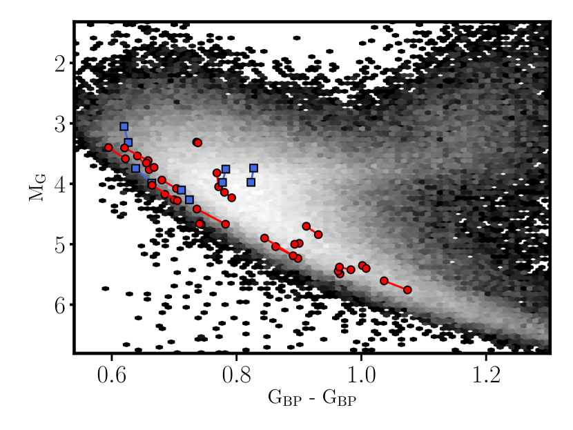
Figure 1: The absolute magnitude in the $G$ band, M_G, as a function of colour ($BP-RP$) for the observed co-moving pairs which turn out to be chemically homogeneous (red circles where pairs are connected by solid lines) and those which have $\Delta$[Fe/H] larger than 0.10 dex (blue squares where pairs are connected by solid lines). For reference, the absolute magnitude in the $G$ band as a function of colour ($BP-RP$) of the GALAH survey crossmatch with Gaia DR2 (with parallax uncertainties better than 10% and parallaxes larger than 1) is also shown as the grayscale background.

In order to determine the level of chemical homogeneity in co-moving binary stellar systems, we started with the set of main-sequence/main-sequence (MS/MS) co-moving pairs identified in El-Badry & Rix (2018). We summarize the method of these authors here. In El-Badry & Rix (2018), the authors identified $\sim 50\times 10^{4}$ MS/MS wide binaries within 200 pc with projected separations between 50 $<s<$ 50000 AU with less than 1% contamination. After doing an initial quality control cut on the stars within Gaia identified with distances less than 200 pc, they do an initial search for companions around each star by (i) rejecting any companions whose parallaxes were inconsistent with that of the primary at the 3-sigma level, and (ii) requiring that the difference in the proper motions of the two stars in the pair be consistent with a bound Keplerian orbit. The authors then removed clusters, moving groups and higher-order multiples outside of pairs of two stars. For a more detailed discussion on the identification of wide binaries, the removal of higher-order multiples, and the expected contamination rate we refer the reader to section 2 of El-Badry & Rix (2018).

We applied several additional cuts. In order to focus in this work on stars with similar T_eff, as a way to reduce potential systematics in the derived parameters and abundances (e.g. Andrews et al., 2019b), we required the difference between the $G$ magnitude of both stars in the pair to be less than 0.30 mag and the difference in the $G_{BP}-G_{RP}$ color to also be less than 0.05 mag. The majority of these pairs are part of the excess of photometric “twin” binaries with mass ratios near 1 discussed in El-Badry et al. (2019). This led to an initial sample of 2948 stars across 1474 co-moving pairs. Of these stars, we were able to observe 50 stars across 25 co-moving pairs at McDonald Observatory in January 2019 (more details in section 2.2). They were selected by prioritizing the bright stars while trying to span a range of projected separations. They were also selected to be far enough apart to minimize light from the companion entering the slit. These stars are typically brighter than G$\sim$ 12 mag. A color magnitude diagram (in M_G as a function of $BP-RP$ for the observed co-moving pairs (red and blue circles) can be found in Fig. 1.

2.2 High Resolution Spectra From McDonald Observatory

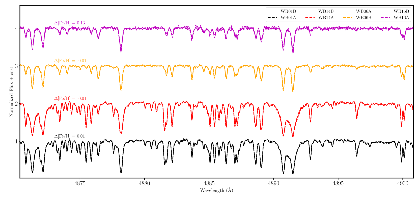
Figure 2: Here we show the observed spectra in the spectra region between 4870–4905 Å of 4 wide binary systems shown as different colours. One component of the binary system is shown as a dotted line, while its companion is shown as a solid line. The difference in [Fe/H] between these spectra are also shown. The spectra of these representative wide binary systems are remarkably similar, except for WB16. As is shown this is one pair where the metallicity is different between the two stars by 0.13 dex

In order to quantify the level of chemical homogeneity, we observed 50  stars across 25 co-moving pairs initially identified in El-Badry & Rix (2018) with the Tull Echelle Spectrograph (Tull et al., 1995) on the 2.7m Harlan J. Smith Telescope at McDonald Observatory in early 2019. The sample size was selected to be comparable to current studies of co-moving pairs of stars (e.g. Oh et al., 2018; Simpson et al., 2018; Andrews et al., 2019a). These observations enabled us to obtain high-resolution (with a resolving power of R $=\lambda/\Delta\lambda\sim$ 60000) optical spectra. We also obtained standard calibration exposures (i.e. biases, flats, and wavelength comparison, ThAr, lamps). The spectra were reduced in the standard way including subtraction of the bias, dividing by the flat field, optimal spectra extraction and scattered light subtraction. In order to stitch the various echelle orders together, we did an initial continuum normalization assuming a fifth order spline function. These processes were done using the echelle package with IRAF. Radial Velocity (RVs) for the spectra were determined by cross correlation with a solar spectral template with the iSpec package (Blanco-Cuaresma et al., 2014). If multiple spectra were observed for the same target, these spectra were co-added (after barycentric correction) in order to obtain the highest SNR possible. For all 25 pairs, the RVs, reported in Table 1, of the two components are within a few km s^-1 of one another and are thus consistent with bound Keplerian orbits. RVs were not used in selecting the wide binaries, so this validates their status as genuine binaries.

Table 1: Observational Properties of Wide Binary Systems

Gaia	RA	DEC	Name	RV	$\sigma$RV	SNR	$\varpi$	PMRA	PMDEC	$G$	$BP-RP$	Teff,phot
	∘	∘		km s-1	km s-1	pixel-1	$\mathrm{mas}$	$\mathrm{mas\,yr^{-1}}$	$\mathrm{mas\,yr^{-1}}$	$\mathrm{mag}$	$\mathrm{mag}$	$\mathrm{K}$
1019003329101872896	140.6659	50.6039	WB01A	4.74	0.08	87	15.05	52.62	9.94	8.95	0.93	5604
1019003226022657920	140.6570	50.6038	WB01B	4.45	0.07	83	15.02	55.93	10.34	8.82	0.91	5663
1448493530351691520	203.6017	26.2772	WB02A	-4.63	0.21	121	7.73	9.77	1.42	8.87	0.63	6460
1448493427272476288	203.5992	26.2761	WB02B	-4.51	0.22	142	7.78	9.74	1.02	8.60	0.62	6360
219605599154126976	57.9389	34.8895	WB03A	12.42	0.36	98	7.26	-9.69	-14.11	9.63	0.68	6440
219593745044391552	57.9426	34.8830	WB03B	12.60	0.28	111	7.21	-9.70	-12.45	9.79	0.70	6461
232899966044906496	63.9372	45.3918	WB04A	65.15	0.10	121	12.91	130.58	-205.86	8.68	0.79	5828
232899966044905472	63.9385	45.3929	WB04B	65.14	0.10	98	12.95	126.08	-203.09	8.58	0.78	5886
238164255921243776	53.8536	42.3046	WB05A	17.58	0.11	87	6.07	1.59	-39.61	10.06	0.82	6027
238163534366737792	53.8673	42.3006	WB05B	17.11	0.11	78	5.96	2.78	-39.37	9.86	0.83	5995
2493516351151864960	36.2245	-2.1121	WB06A	26.25	0.17	114	8.17	70.17	-13.37	8.98	0.64	6302
2493516351151865088	36.2224	-2.1122	WB06B	26.51	0.15	124	8.15	69.20	-14.46	9.21	0.66	6251
2565584837226776448	24.4075	7.1462	WB07A	23.71	0.08	74	14.58	79.89	-79.66	9.58	1.01	5247
2565584802867037696	24.4184	7.1488	WB07B	24.59	0.07	68	14.48	80.61	-78.94	9.55	1.00	5250
2572433351559023616	26.0631	9.4849	WB08A	7.11	0.29	140	13.80	139.94	-68.27	7.89	0.62	6513
2572433347264096768	26.0639	9.4838	WB08B	7.79	0.43	97	13.72	142.94	-67.96	7.71	0.59	6682
2573278051366910336	25.3299	10.1139	WB09A	18.91	0.13	118	12.18	161.36	34.43	8.68	0.71	5908
2573278120086386432	25.3244	10.1179	WB09B	18.95	0.14	120	12.25	159.97	35.27	8.82	0.72	6091
271977330850893568	65.6146	51.8143	WB10A	14.94	0.15	92	8.85	23.35	-47.27	9.93	0.78	6242
271977330850895488	65.6106	51.8089	WB10B	15.59	0.11	80	8.90	21.34	-48.69	9.67	0.74	6025
3097066080667487488	125.7440	7.6303	WB11A	-15.38	0.09	97	19.62	13.90	-19.06	8.98	0.96	5479
3097066080667486592	125.7474	7.6308	WB11B	-14.76	0.09	97	19.66	16.17	-21.31	9.02	0.97	5355
3170300942420466176	112.4253	18.2757	WB12A	-26.74	0.12	110	8.07	-8.96	-31.39	9.28	0.77	5913
3170394607068638336	112.4483	18.2795	WB12B	-26.52	0.11	105	8.13	-8.81	-31.62	9.50	0.77	5916
3230677870385455232	69.3588	0.5747	WB13A	39.18	0.13	129	15.60	15.95	12.16	7.36	0.74	5864
3230677565443833088	69.3614	0.5532	WB13B	39.15	0.14	134	15.59	16.65	11.60	7.34	0.74	5865
3288572968680438912	73.5689	7.3680	WB14A	47.57	0.08	101	33.78	246.13	-197.63	8.11	1.07	5193
3288572968680438528	73.5704	7.3722	WB14B	47.41	0.08	101	33.75	248.06	-202.01	7.96	1.04	5226
3391840612589045632	77.5610	13.9951	WB15A	37.16	1.45	154	9.68	13.57	-10.18	8.48	0.62	6519
3391840539572707072	77.5628	13.9880	WB15B	37.40	0.18	133	9.49	13.32	-11.56	8.73	0.66	6493
3588936180766441600	177.0016	-8.6279	WB16A	-19.04	0.25	71	7.26	61.62	-47.01	9.44	0.64	6258
3588936180766441728	176.9990	-8.6263	WB16B	-18.71	0.17	60	7.32	62.40	-47.03	9.67	0.66	6354
3644886925888351872	209.0257	-4.6167	WB17A	8.34	0.20	46	9.01	-11.39	26.99	8.96	0.67	6095
3644886925888352000	209.0271	-4.6159	WB17B	7.24	0.24	67	8.91	-10.73	26.60	8.91	0.66	6265
3890860183966486656	156.7826	18.0623	WB18A	12.03	0.08	88	17.48	-124.03	-105.54	9.21	0.98	5347
3890860179670959104	156.7845	18.0619	WB18B	11.86	0.08	93	17.48	-124.84	-112.56	9.17	0.96	5404
3975129194660883328	178.6316	19.4112	WB19A	6.52	0.10	126	25.24	-450.50	-16.55	8.03	0.86	5739
3975223065466473216	178.6441	19.4278	WB19B	6.31	0.09	125	25.25	-450.60	-15.50	8.22	0.90	5607
4024887730814401280	174.7115	32.6420	WB20A	22.88	0.15	113	7.51	-94.48	44.03	9.89	0.70	6195
4024886425144354816	174.6790	32.6261	WB20B	20.57	0.14	114	7.56	-95.34	43.59	9.78	0.69	6283
440947391590004096	46.0106	52.5151	WB21A	-38.83	0.16	98	7.10	23.25	25.53	9.50	0.78	5947
440959142620525568	46.0079	52.5165	WB21B	-39.66	0.16	80	7.07	23.64	24.43	9.73	0.78	6040
478240661338191360	75.8897	63.0873	WB22A	-25.49	0.09	123	31.08	101.97	316.19	7.44	0.84	5514
478240661338195328	75.8793	63.0795	WB22B	-24.84	0.10	136	31.04	105.90	311.37	7.73	0.89	5687
692119656035933568	137.0992	27.5357	WB23A	31.05	0.12	111	20.45	-53.24	71.66	8.11	0.74	5996
692120029700390912	137.1129	27.5434	WB23B	31.31	0.13	116	20.36	-51.82	73.52	8.13	0.74	5974
736174028943041920	159.8656	31.7048	WB24A	9.22	0.10	97	14.48	-110.90	-36.06	9.20	0.89	5632
736173925863826944	159.8621	31.7008	WB24B	8.65	0.09	83	14.43	-112.71	-36.51	9.19	0.90	5605
914241517609344128	126.7051	39.0131	WB25A	-3.33	0.20	114	11.64	27.13	5.81	8.69	0.66	6430
914244399532441472	126.6368	39.0493	WB25B	-3.09	0.16	127	11.72	27.62	6.36	8.93	0.71	6232

NOTE: The Gaia DR2 source identifier of each star is given in column 1 with sky coordinates in columns 2 and 3. The associated wide binary component of each star is listed in column 4. The radial velocity and its uncertainty measured in our optical spectra are given columns 5 and 6, respectively. The signal-to-noise ratios (SNR), measured in at the continuum level at $\sim$5350Å, of our optical spectra are listed in column 7. The parallax and proper motion in RA and DEC are given in columns 8, 9, and 10, respectively. The $G$ band magnitude and $(BP-RP)$ colour are given in columns 11 and 12, respectively. Finally the Gaia derived photometric temperatures (Andrae et al., 2018) are given in the last column.

The final reduced spectra have wavelength coverage $\sim$3500-10000 Å over $\sim$60 echelle orders with some inter-order gaps, particularly in the redder wavelengths. In Table 1, we report the basic observational properties (i.e. Gaia DR2 source identified numbers, sky positions, parallaxes, proper motions, radial velocities, photometry) of our sample. We also report the photometric T_eff provided by Gaia (their teff_val column, Andrae et al., 2018) in order to compare to the temperatures derived spectroscopically in this work. The typical uncertainty on the photometric T_eff values derived from Gaia are on the order of $\sigma$T_eff $\sim$150 K.

We primarily obtained high signal-to-noise ratio (SNR $>$ 60 pixel^-1) for each star in the 25 co-moving pair in order to precisely quantify their chemical abundance pattern. We note that the typical (mean) SNR is $\sim$ 105 pixel^-1 ensuring that we can obtain high fidelity chemical abundance estimates. In Fig. 2 we show sample spectra of 4 pairs. It is interesting to already note that the spectra of the various pairs look remarkably similar.

3 Stellar Parameter and Abundance Analysis

Stellar parameters were determined in an automatic fashion under the standard Fe excitation-ionization balance technique using the ‘param’ module of the Brussels Automatic Code for Characterizing High accUracy Spectra (BACCHUS, Masseron et al., 2016) code. Similar to Hawkins & Wyse (2018), we used the version of BACCHUS which includes the MARCS model atmosphere grid (Gustafsson et al., 2008), along with TURBOSPECTRUM (Alvarez & Plez, 1998; Plez, 2012), which is used to generate synthetic spectra under the assumption of Local Thermodynamic Equilibrium (LTE). The atomic data (line list) are taken from the fifth version of the Gaia-ESO linelist (Heiter et al., 2019). Molecular species were also included. The molecular species added include: CH (Masseron et al., 2014), and CN, NH, OH, MgH and C₂(T. Masseron, private communication). SiH molecules are adopted from the Kurucz linelists and those from TiO, ZrO, FeH, CaH from B. Plez (private communication) are also included. We note that hyperfine structure splitting is included for Sc I, V I Mn I, Co I, Cu I, Ba II, Eu II, La II, Pr II, Nd II, Sm II (Heiter et al., 2019). The synthetic spectra produced using the above procedure are then compared via $\chi^{2}$ minimization to the observed spectra. We note here that instrument, rotational, and macroturbulent broadening are also included during the spectral synthesis and derived by ensuring that the abundance determined from the $\chi^{2}$ minimization matches the abundances determined using the core of the line (Masseron et al., 2016). The line selection for each element was done in the same way as in Hawkins et al. (2015).

Under the standard Fe excitation-ionization balance procedure we derived the T_eff  by ensuring that there is no correlation between the abundance of Fe and the excitation potential of the lines being used. On the other hand, log $g$ is derived by forcing no significant offset between the abundance of neutral Fe (Fe i) and that of singly ionized Fe (Fe ii). Further, the microturbulent velocity parameter $\xi$ is determined by ensuring there to be no correlation between the abundance of Fe and the reduced equivalent width (REW, defined as equivalent width divided by the wavelength of the line). For this procedure we used up to 100 Fe i lines and 20 Fe ii lines. Individual abundances for 23 elements across the light/odd-Z (Li, C, Na, Al, Sc, V), $\alpha$ (Mg, Si, Ca, Ti), Fe-peak (Cr, Mn, Fe, Co, Ni, Zn), and neutron capture (Sr, Y, Zr, Ba, La, Nd, Eu) families were derived using the ‘abund’ module within BACCHUS. This module derives abundances by first fixing the stellar atmospheric parameters to those derived as described using Fe excitation-ionization balance and then synthesizing spectra with different values of [X/H]. The reported [X/H] abundance was determined using a $\chi^{2}$ minimization between these synthetic and observed spectra. For more details about BACCHUS, we refer the reader to Section 2.2 of Hawkins et al. (2015). We note that the solar abundances from Asplund et al. (2005) are assumed. The total internal uncertainty in the derived abundances is important to quantify in order to determine with what precision we can conclude the chemical homogeneity of wide binary systems. In order to derive an estimate of the total internal uncertainty in stellar abundances, we follow Hawkins et al. (2016) where we first quantify the representative sensitivity of each of the chemical abundances to the uncertainty in the stellar atmospheric parameters (T_eff, log $g$, $\xi$). This is effectively equivalent to propagating the uncertainty in the stellar parameters through to the chemical abundances. The sensitivity of the abundance ratios, [X/H], due to uncertainties in the T_eff, log $g$, and $\xi$ are then added in quadrature with standard error in the mean of the individual absorption features used to determine the abundance (e.g. Desidera et al., 2004; Desidera et al., 2006; Yong et al., 2013; Roederer et al., 2014; Hawkins et al., 2016; Lucey et al., 2019). We note here that, in principle, this method for estimating the uncertainty in the stellar abundances neglect the covariances between the stellar parameters and treats them independently (e.g. see McWilliam et al., 1995, for a longer discussion on this). In Table 2, we tabulate the typical (conservative) sensitivities (i.e. the median difference in [X/H]) due to an uncertainty in T_eff of 100 K, in log $g$ of 0.25 dex, and $\xi$ of 0.10 km s^-1. These typical uncertainties are computed as the mean of the T_eff, log $g$, [Fe/H], and $\xi$ uncertainty which is an output of the ‘param’ module within BACCHUS. For this calculation, we choose to compute the sensitivities for 8 stars across 4 binary systems that span our T_eff-log $g$-[Fe/H] parameter range. The median difference in [X/H] as a result of perturbing the stellar parameters by their uncertainties can be found in Table 2.

Table 2: Stellar abundance sensitivities to the uncertainty in the stellar parameters

$\Delta$[X/H]	$\Delta$Teff	$\Delta$log $g$	$\Delta$$\xi$
	($\pm$100 K)	($\pm$0.25 dex)	($\pm$0.10 km s-1)
Li	$\pm$0.07	$\pm$0.00	$\mp$0.00
C	$\pm$0.11	$\mp$0.02	$\mp$0.00
Na	$\pm$0.06	$\mp$0.03	$\mp$0.00
Mg	$\pm$0.11	$\mp$0.10	$\mp$0.01
Al	$\pm$0.04	$\pm$0.00	$\mp$0.00
Si	$\pm$0.03	$\pm$0.02	$\mp$0.02
Ca	$\pm$0.06	$\mp$0.02	$\mp$0.02
Sc	$\pm$0.03	$\pm$0.07	$\mp$0.03
Ti	$\pm$0.10	$\pm$0.01	$\mp$0.03
V	$\pm$0.12	$\pm$0.01	$\mp$0.00
Cr	$\pm$0.08	$\mp$0.01	$\mp$0.02
Mn	$\pm$0.09	$\mp$0.01	$\mp$0.02
Fe	$\pm$0.06	$\pm$0.01	$\mp$0.02
Co	$\pm$0.08	$\pm$0.03	$\pm$0.00
Ni	$\pm$0.07	$\mp$0.01	$\mp$0.02
Cu	$\pm$0.07	$\pm$0.01	$\mp$0.01
Zn	$\pm$0.03	$\pm$0.02	$\mp$0.01
Sr	$\pm$0.10	$\pm$0.03	$\pm$0.01
Y	$\pm$0.02	$\pm$0.07	$\mp$0.03
Zr	$\pm$0.05	$\pm$0.05	$\mp$0.00
Ba	$\pm$0.04	$\pm$0.01	$\mp$0.05
La	$\pm$0.05	$\pm$0.07	$\mp$0.01
Nd	$\pm$0.04	$\pm$0.06	$\mp$0.00
Eu	$\pm$0.01	$\pm$0.09	$\mp$0.01

NOTE: The change in [X/H] abundance (denoted in column 1) when the T_eff is perturbed by $\pm$100 K (column 2), log $g$ is perturbed by $\pm$0.25 dex (column 3), $\xi$ is perturbed by $\pm$0.10 km s^-1(column 4). Total uncertainties are obtained by adding these in quadrature with the standard error in the line-by-line abundances.

4 Results and Discussion

In this section, we present the results of our stellar parameter and abundance analysis and critically focus on the difference in chemical abundance ratios, i.e. $\Delta$[X/H] and $\Delta$[X/Fe], between the two stars in the 25 wide binary systems. We also intermix these results with a discussion placing these results in the context of recent studies on the homogeneity of wide binary systems. We start by presenting the stellar parameters for each of the 50 observed stars in the 25 binary systems in section 4.1. We then move on to discuss the differences in the [X/H, Fe] abundance ratios for wide binaries compared to random pairings of stars in light and odd-Z elements (section 6), $\alpha$ elements (section 4.3), Fe-peak elements (section 4.4), and neutron capture elements (section 4.5).

Table 3: Stellar Parameter and Chemical Abundance Ratios of Observed Wide Binary Systems

Source ID	Name	Teff	$\sigma$Teff	log $g$	$\sigma$log $g$	[Fe/H]	$\sigma$[Fe/H]	$\xi$	$\sigma$$\xi$	[Si/H]	$\sigma$[Si/H]	…
		(K)	(K)	(dex)	(dex)	(dex)	(dex)	(km s-1)	(km s-1)	(dex)	(dex)
1019003329101872896	WB01A	5604	24	4.62	0.07	0.36	0.01	0.87	0.05	0.41	0.03	…
1019003226022657920	WB01B	5663	21	4.67	0.12	0.37	0.01	1.03	0.05	0.34	0.03	…
1448493530351691520	WB02A	6460	54	3.96	0.45	-0.11	0.01	1.47	0.08	-0.21	0.02	…
1448493427272476288	WB02B	6360	95	3.94	0.19	-0.21	0.01	1.62	0.09	-0.22	0.04	…
219605599154126976	WB03A	6440	38	4.36	0.34	-0.35	0.02	1.09	0.11	-0.29	0.05	…
219593745044391552	WB03B	6461	64	4.56	0.68	-0.34	0.01	1.47	0.14	-0.34	0.05	…
232899966044906496	WB04A	5828	31	4.35	0.20	-0.00	0.01	1.17	0.05	0.03	0.03	…
232899966044905472	WB04B	5886	29	4.44	0.29	0.04	0.01	1.16	0.05	0.05	0.02	…
238164255921243776	WB05A	6027	29	4.29	0.31	0.20	0.01	1.25	0.04	0.18	0.03	…
238163534366737792	WB05B	5995	68	4.32	0.44	0.09	0.01	1.32	0.05	0.14	0.03	…
2493516351151864960	WB06A	6302	108	4.22	0.26	-0.20	0.01	1.54	0.07	-0.19	0.03	…
2493516351151865088	WB06B	6251	52	4.30	0.49	-0.19	0.01	1.36	0.06	-0.17	0.03	…
2565584837226776448	WB07A	5247	22	4.67	0.20	0.14	0.01	0.70	0.04	0.20	0.04	…
2565584802867037696	WB07B	5250	21	4.56	0.23	0.13	0.01	0.88	0.04	0.19	0.04	…
2572433351559023616	WB08A	6513	44	4.07	0.85	-0.06	0.01	1.37	0.07	-0.07	0.04	…
2572433347264096768	WB08B	6682	15	4.39	0.49	-0.07	0.02	1.35	0.12	0.01	0.04	…
2573278051366910336	WB09A	5908	61	4.31	0.28	-0.28	0.01	1.27	0.06	-0.23	0.03	…
2573278120086386432	WB09B	6091	39	4.31	0.39	-0.16	0.01	1.24	0.06	-0.19	0.02	…
271977330850893568	WB10A	6242	32	4.83	0.28	-0.01	0.01	1.22	0.06	-0.08	0.04	…
271977330850895488	WB10B	6025	17	4.80	0.28	0.02	0.01	1.02	0.04	-0.09	0.04	…
3097066080667487488	WB11A	5479	65	4.78	0.33	-0.01	0.01	1.52	0.05	-0.05	0.03	…
3097066080667486592	WB11B	5355	57	4.75	0.01	-0.06	0.01	1.20	0.05	-0.02	0.03	…
3170300942420466176	WB12A	5913	24	4.21	0.17	-0.20	0.01	1.13	0.05	-0.20	0.02	…
3170394607068638336	WB12B	5916	14	4.27	0.25	-0.16	0.01	1.04	0.04	-0.22	0.02	…
3230677870385455232	WB13A	5864	69	3.92	0.10	-0.30	0.01	1.37	0.06	-0.22	0.03	…
3230677565443833088	WB13B	5865	24	3.79	0.21	-0.33	0.01	1.31	0.08	-0.28	0.03	…
3288572968680438912	WB14A	5193	68	4.50	0.44	0.07	0.01	1.22	0.04	0.01	0.03	…
3288572968680438528	WB14B	5226	38	4.65	0.07	0.06	0.01	1.13	0.04	0.09	0.03	…
3391840612589045632	WB15A	6519	65	4.38	0.26	0.13	0.01	1.57	0.09	0.10	0.02	…
3391840539572707072	WB15B	6493	69	4.34	0.31	0.12	0.01	1.55	0.08	0.09	0.02	…
3588936180766441600	WB16A	6258	47	4.13	0.26	-0.30	0.01	1.39	0.09	-0.25	0.03	…
3588936180766441728	WB16B	6354	51	4.44	0.49	-0.17	0.01	1.31	0.10	-0.21	0.03	…
3644886925888351872	WB17A	6095	106	4.06	0.34	-0.00	0.02	1.55	0.09	0.01	0.02	…
3644886925888352000	WB17B	6265	83	4.15	0.34	0.01	0.01	1.71	0.07	-0.02	0.04	…
3890860183966486656	WB18A	5347	64	4.60	0.32	0.07	0.01	1.10	0.04	0.06	0.03	…
3890860179670959104	WB18B	5404	17	4.64	0.32	0.05	0.01	1.05	0.03	0.05	0.03	…
3975129194660883328	WB19A	5739	25	4.69	0.23	-0.07	0.01	1.00	0.05	-0.10	0.02	…
3975223065466473216	WB19B	5607	14	4.75	0.12	-0.04	0.01	0.76	0.05	-0.09	0.03	…
4024887730814401280	WB20A	6195	25	4.47	0.30	-0.16	0.01	1.10	0.06	-0.22	0.02	…
4024886425144354816	WB20B	6283	26	4.55	0.30	-0.14	0.01	1.19	0.06	-0.18	0.03	…
440947391590004096	WB21A	5947	129	4.16	0.23	-0.66	0.01	1.59	0.15	-0.59	0.03	…
440959142620525568	WB21B	6040	45	4.21	0.31	-0.58	0.01	1.20	0.13	-0.54	0.03	…
478240661338191360	WB22A	5514	26	4.64	0.21	-0.22	0.01	1.01	0.05	-0.19	0.03	…
478240661338195328	WB22B	5687	25	4.57	0.38	-0.21	0.01	1.06	0.04	-0.19	0.02	…
692119656035933568	WB23A	5996	30	4.62	0.22	-0.26	0.01	1.07	0.06	-0.31	0.02	…
692120029700390912	WB23B	5974	68	4.51	0.33	-0.28	0.01	1.30	0.05	-0.33	0.03	…
736174028943041920	WB24A	5632	45	4.63	0.35	0.17	0.01	1.13	0.04	0.13	0.03	…
736173925863826944	WB24B	5605	50	4.63	0.38	0.19	0.01	1.17	0.04	0.17	0.03	…
914241517609344128	WB25A	6430	37	4.59	0.23	-0.04	0.01	1.28	0.07	-0.12	0.03	…
914244399532441472	WB25B	6232	34	4.64	0.20	-0.10	0.01	1.29	0.09	-0.12	0.03	…

NOTE: This is a subsample of the spectroscopically derived stellar parameters (T_eff, log $g$, [Fe/H], $\xi$) and the chemical abundances [X/H] for the 50 stars in our sample. The full table will be provided in the online material. The Gaia DR2 source identifier and the wide binary name of each star is given in columns 1 and 2. The stellar parameters and their uncertainties (T_eff, $\sigma$T_eff, log $g$, $\sigma$log $g$, [Fe/H](where [Fe/H] is measured by [Fe I/H]), $\sigma$[Fe/H], $\xi$, $\sigma$$\xi$) are found in columns 3-10, respectively. The chemical abundance ratio for [Si/H] is found in column 11 and its uncertainty in column 12. We note that this uncertainty is determined as the dispersion in the [Si/H] over all lines used to derive [Si/H] divided by the square root of the number of lines used.

4.1 Stellar Atmospheric Parameters

The stellar atmospheric parameters and chemical abundances, denoted [X/H], can be found in Table 3. More specifically, the derived stellar parameters, and their uncertainties are reported in the first eight columns after the identifiers in Table 3. Typical errors in T_eff, log $g$, [Fe/H], and $\xi$ are approximately $\sim$40 K, 0.25 dex, 0.01 dex (line-by-line), and 0.06 km s^-1, respectively. Additionally, the chemical abundances (reported as [X/H]) for 23 elemental species for each star in our sample can also be found in Table 3. These are determined by taking the median of the [X/H] abundances in ‘clean’ absorption features found by the BACCHUS ‘abund’ module.

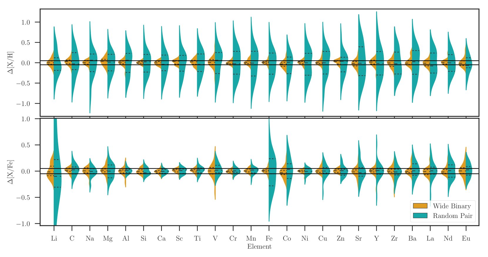
Figure 3: Top: Violin diagram showing the distribution of the difference in [X/H] for the 23 reported elemental species between the two components of the 25 wide binary pairs (orange). Also shown is the distribution of the difference in [X/H] between each star and the closest star on the color-magnitude diagram (Fig. 1), which is not its companion (cyan). Bottom: The same as the top panel but now showing the difference in [X/Fe] instead of [X/H]. For reference, dashed lines denote the (inner, outer and median) quartiles and solid lines in both panels are shown at $\Delta$[X/Fe] = $\pm$0.05 and $\Delta$[X/H] = $\pm$0.05 dex. For reference, in the bottom panel, Fe represents the difference in the [Fe/H].

The uncertainties of the reported [X/H] abundances in that table are derived by taking the standard deviation in the line-by-line [X/H] abundances and dividing by the square root of the number of lines used (i.e. the standard error in the mean). Where only one line is able to be measured the uncertainty is conservatively assumed to be $\pm$0.10 dex. The total abundance uncertainty is determined by adding, in quadrature, the uncertainty in mean [X/H], which is reported in Table 3, along with each of the typical sensitivities of the abundance ratio with respect to the stellar parameters, reported in Table 2. The median total abundance uncertainty across all elements is on the order of $\sim\pm$0.08 dex.

In practice, for both chemical tagging and characterization of exotic (M-dwarf, white-dwarf, etc.) stars using wide binaries to work, the difference in [X/H], or conversely [X/Fe], between the two stars in the pair must be consistent with zero. In this case, both stars in the wide binary pair would be chemically identical. Therefore, the distribution of difference for each chemical element ratio (with the $\Delta$[X/H] in the top panel and $\Delta$[X/Fe] in the bottom panel) between the wide binary pairs (orange) in this work are shown as a violin diagram in Fig. 3. For each element, we take the [X/H, Fe] ratio of component A and subtract it from the [X/H, Fe] ratio of component B. Stars in each pair were randomly assigned an ‘A’ or ‘B’ label. For reference, we also show in cyan the distribution of the difference in [X/H] (top) and [X/Fe] (bottom) between one star in each pair and the closest star in color-magnitude space that is not its companion. This can be thought of as a ‘random pairing’ of stars which also happen to have similar T_eff. We choose only one star per pair to match with a random star to in order to consistently compare 25 random pairs to 25 wide binary pairs. This was done to compare the chemical homogeneity of random pairings of field stars of similar stellar parameters but not born together to those wide binary systems which are likely born together. For reproducibility, we have identified the random pair combinations used for this work in Table 3. We also note here the key results do not change by using completely random pairs versus those which are random but also close-by in colour-magnitude space.

Figure 4: The difference in the metallicity, $\Delta$[Fe/H], of both components of the wide binary as a function of the projected separation between the components. Each pair is colour-coded by the difference in the T_eff between the stars of the pair.

Focusing first on the wide binaries, in Fig. 3 we find that the distribution in $\Delta$[Fe/H] is centered at $\Delta$[Fe/H] $\sim$0.00 dex with a dispersion of 0.05 dex. We note however, that there is a component (which accounts for 80% of the sample, 20/25 systems) that is chemically homogeneous, with a median $\Delta$[Fe/H] $\sim$0.01 dex and a dispersion of 0.02 dex and a second component (20% of the sample or 5/20 systems) of chemically similar, but not homogeneous, wide binaries with a median $\Delta$[Fe/H] $\sim$0.11 dex and a dispersion of 0.04 dex. Fig. 4 shows the difference in [Fe/H] between wide binary pairs as a function of their separation. The projected separations are taken from El-Badry & Rix (2018). This figure indicates that the five systems which have $\Delta$[Fe/H] $>$ 0.10 dex are not at systematically larger separations compared to those which are chemically alike (with $\Delta$[Fe/H] $<$ 0.01 dex). In a forthcoming work, we will explore pairs with separation $>10^{4}$ AU (Ting, Ji, Hawkins, in preparation).

This result indicates that the occurrence of wide binaries which have large abundance difference is not a common event. Our results also indicate that wide binary systems are commonly homogeneous to within $\pm$0.02 dex in [Fe/H]. This is consistent with and builds on what has been found in other studies (e.g. Desidera et al., 2004; Desidera et al., 2006; Andrews et al., 2017, 2019a). Interestingly, in a smaller sample of 8 wide binaries, Simpson et al. (2018) found that abundance differences between components of wide binary systems observed in the GALAH survey are much more common. This could be due to the fact these authors compare wide binary pairs which have very different effective temperatures ($\Delta$T_eff$>$ 200 K). This is known to induce larger abundance differences (Andrews et al., 2019a).

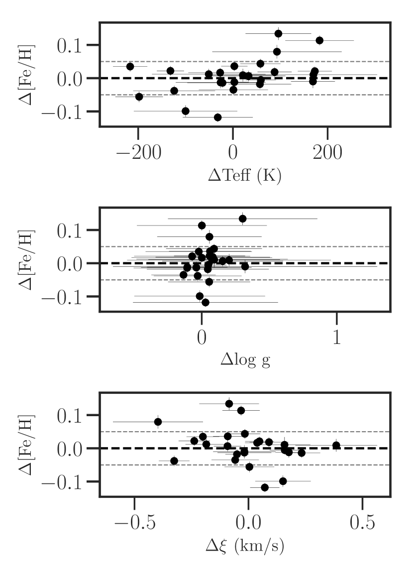
Figure 5: Top: The difference in [Fe/H] between wide binary pairs as a function of the difference in their T_eff. Middle: The difference in [Fe/H] between wide binary pairs as a function of the difference in their log $g$. Bottom: The difference in [Fe/H]  as a function of the difference in their $\xi$.

It is possible that there are systematic issues with the T_eff for the outlier population. Therefore, to ensure that the pairs with $\Delta$[Fe/H] $>\pm$ 0.10 dex are reliable, in Fig. 5, we show the difference in the [Fe/H] for each wide binary system as a function of the difference in the $\Delta$T_eff (top panel), $\Delta$log $g$ (middle panel), $\Delta$$\xi$(bottom panel). We do this as a way to determine whether the outlier wide binary systems, which are different in [Fe/H]  with $\Delta$[Fe/H]$>$ 0.10 dex, are a result of the systematics induced by the differences in the stellar parameters between the two stars. Fig. 5 show that there are no correlations between the difference in [Fe/H] and the differences in the remaining stellar parameters. Additionally, in Fig. 6 we show the difference in the photometric T_eff determined from Gaia (Andrae et al., 2018), and the spectroscopic T_eff derived in this work as a function of the spectroscopic T_eff. The median offset between the photometric and spectroscopic T_eff is $\sim$60 K with a dispersion of 130 K. This offset is consistent with other (optical) spectroscopic T_eff comparisons with photometric T_eff scales (e.g. Bergemann et al., 2014). Finally, in Fig. 2, in magenta, we show the spectra of one of the wide binary pairs with $\Delta$[Fe/H] $>$ 0.10 dex compared with spectra from other wide binary pairs which are chemically homogeneous. The spectra between the two stars in WB16 (shown as the magenta solid and dotted lines) are significantly different in the strength of their absorption features, unlike the remaining wide binary pairs. This is to say the spectra for wide binaries that have $\Delta$[Fe/H] $>$ 0.10 dex are visibly different compared to those that are not.

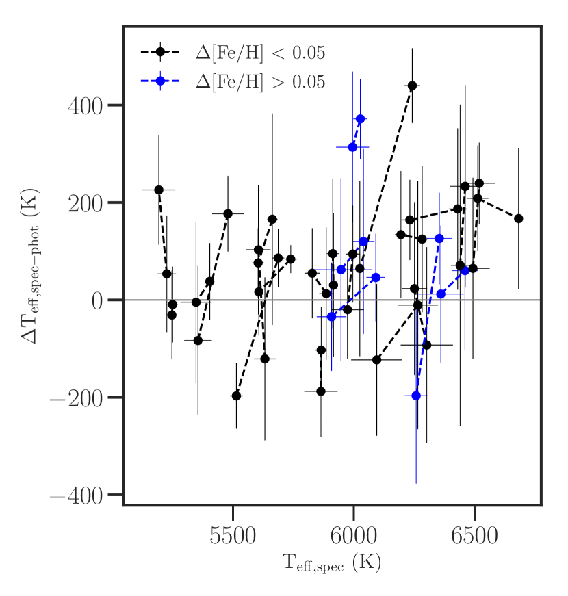
Figure 6: The difference in the photometrically-derived T_eff and the spectroscopically derived T_eff, $\Delta$T_eff, as a function of the spectroscopic T_eff. Each star in the wide binary pair is connected using a dotted line. Wide binaries with differences in [Fe/H] less than 0.05 dex are shown in black while those with $\Delta$[Fe/H] $>$ 0.05 dex are shown in blue.

4.2 Light/odd-Z elements (Li, C, Na, Al, Sc, V, Cu)

We determined the abundance of the light element Li using the absorption feature at 6707.8 Å. Reassuringly, we find that the abundance of lithium, A(Li), of our stars follows a similar trend with T_eff as expected for typical FGK dwarf stars, namely that A(Li) tends to decrease with decreasing T_eff and plateaus above T_eff $\leq$ 6200 K (e.g. Ramírez et al., 2012). In Fig. 7, we show the abundance of Li, i.e. A(Li) = [Li/H] + 1.05 (where 1.05 is the solar Li abundance, Asplund et al., 2005), for our wide binary stars in black compared to a sample of stars from the Galactic disk from Ramírez et al. (2012). This figure illustrates two important points: (1) Our sample of wide binaries follows the typical trend in T_eff dependent depletion as found in the Galactic disk, and (2) if one selects wide binaries with very different T_eff it may not be expected for their A(Li), and therefore their [Li/H] or [Li/Fe], to be equal. This also may explain why the dispersion in $\Delta$[Li/H] (and subsequently $\Delta$[Li/Fe]) abundance ratios are larger than for other elements.

Figure 7: The abundance of Li, denoted as A(Li), as a function of T_eff in K for our wide binary stars (shown in black), compared to a sample of stars from the Galactic disk from Ramírez et al. (2012) in in gray.

Furthermore, we find that the typical difference in Li between the two wide binary pairs is $\Delta$A(Li) = 0.00 with a dispersion of 0.09 dex. For the purposes of this discussion, we show in Fig. 8 the dispersion in the difference of [X/H], i.e. $\sigma\Delta$[X/H], as red triangles. Also shown in Fig. 8 is the typical total uncertainty (as black circles) and the dispersion in the difference of [X/H] for random pairs (orange triangles) instead of wide binaries (red triangle). In Fig. 9, we also show the dispersion in the difference of [X/Fe], i.e. $\sigma\Delta$[X/Fe], for the wide binaries in this work (red triangles), the random pairs of stars (as orange triangles). Similar to Fig. 8, we also show the typical uncertainty in [X/Fe], which we approximate as the uncertainty in [X/H] added in quadrature with the uncertainty in [Fe/H] for each star. We note here that this analysis does not account for possible covariances between the uncertainties in [X/Fe] and the stellar parameters. Therefore we caution that the uncertainties quoted in Fig. 9 are conservative. While we add this figure for completeness, we additionally caution that two random stars not born together as a pair in the Galactic thin disk can have very different [Fe/H] but very similar [X/Fe], because the dynamic range in [X/Fe] is on the same order (e.g. $\sim$0.10 dex) as the uncertainty in [X/Fe] (also on the order of $\sim$0.10 dex). This is why [X/H] is critically important for the purposes of chemical tagging.

These two figures together indicate that the dispersion in the difference of [Li/Fe] is slightly larger compared to the dispersion in $\Delta$[Li/H] for the wide binaries, which can be explained by increased uncertainties in [Li/Fe]. However for the random pairs, the dispersion in $\Delta$[Li/Fe] is significantly larger than for $\Delta$[Li/H]. This can be attributed both to (1) increased uncertainties in [Li/Fe] compared to [Li/H] and (2) the fact that the Li abundance depends systematically on T_eff (e.g. Fig. 7) and the random pairs have a large dispersion in T_eff compared to the wide binaries. This T_eff dependent Li depletion illustrates why Li should not generally be used for chemical tagging.

Interestingly, the typical total internal uncertainty in Li is approximately 0.12 dex. We remind the reader this value is derived by adding in quadrature the standard error in the mean of the line-by-line abundances and the sensitivities of the abundance to the stellar parameters. This is in contrast to $\Delta$A(Li) = –0.09 with a significantly larger dispersion of 0.29 dex if one compares each star with the closest star on the CMD, which is not its binary companion. We remind the reader this comparison is a way to quantify the expected difference between random field stars of similar T_eff and log $g$ internally using the results from our spectra.

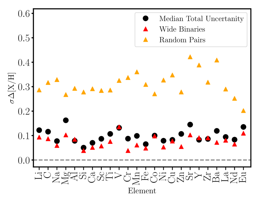
Figure 8: The dispersion in the difference of [X/H] abundance ratios between wide binaries (red triangles) compared to random pairs of stars (orange triangles). For reference, the typical uncertainty in each element is shown as black circles.

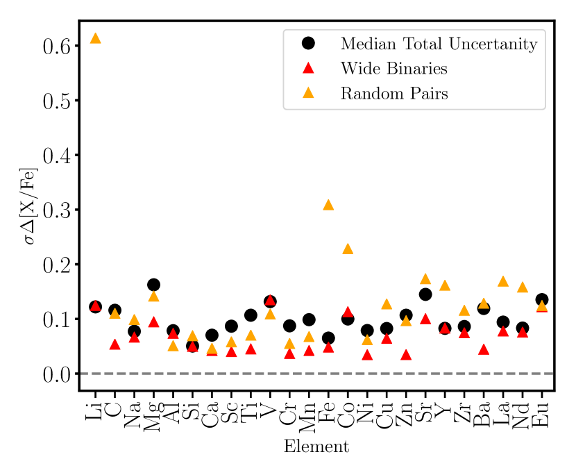
Figure 9: The same as Fig. 8 except for the dispersion in the difference of [X/Fe] abundance ratios instead. As above, for Fe we show the [Fe/H] for comparison.

C is a light element and is determined using a combination of molecular features (namely CH) and two atomic features Nissen et al. (2014). Using these C features, we were able to derive abundances for [C/H] and find that the typical difference between the two stars in the wide binary pairs is $\Delta$[C/H] ($\Delta$[C/Fe]) = 0.02 (0.02) with a dispersion of 0.09 (0.05) dex in [X/H] ([X/Fe]). This is in contrast to $\Delta$[C/H] = –0.03 (0.02) with a larger dispersion of 0.32 (0.11) dex if we were to compare each star with the closest star on the CMD, which is not its binary companion. The median total uncertainty in [C/H] is 0.12 dex, dominated by the propagated uncertainty in [C/H] with respect to T_eff. While there is a noticeable and significant spread of 0.32 dex in $\Delta$[C/H] when comparing random stars of similar spectral type, we find an offset and spread well below the uncertainty for wide binary pairs consistent with wide binaries originating most often in clouds homogeneous in C.

Na, Al, Sc, Cu, and V are all odd-Z elements. We determined the abundance of Na in each star using up to 4 absorption features. We find that the median difference in [Na/H, Fe] is 0.00 (0.00) dex with a dispersion of 0.06 (0.07) dex. This is in contrast to significantly larger differences, $\Delta$[Na/H] = 0.06 (-0.01) with a dispersion of 0.33 (0.10) dex for the random pairs. For reference, the median total uncertainty in [Na/H] is 0.07 dex.

Similarly, for Al, we use up to 2 absorption features. The typical uncertainty in [Al/H] is $\sim$0.08 dex. For the wide binary systems studied here we find that the median $\Delta$[Al/H] = 0.01 (0.00) dex and a dispersion in the difference in [Al/H], i.e. $\sigma\Delta$[Al/H], of 0.08 (0.08) dex. Similar results are also found in Sc where the $\Delta$[Sc/H] = 0.03 (0.01) with a dispersion of 0.06 (0.04) dex. Note that the typical uncertainty in [Sc/H] is 0.09 dex. Significantly larger dispersion in $\Delta$[Al, Sc/H] are detected for random pairs of stars.

Cu, much like the other odd-Z elements, we find to have a median difference in $\Delta$[Cu/H, Fe] is 0.00 (0.00) dex with a dispersion in the difference of $\sigma\Delta$[Cu/H, Fe] is 0.08 (0.06) dex. With a median total uncertainty in [Cu/H] of 0.08 dex, the differences we find between wide binary pairs in [Cu/H, Fe] is likely a result of measurement uncertainty. On the other hand, for the random pairs of stars the median difference in $\Delta$[Cu/H, Fe] is 0.00 (0.00) dex with a dispersion in the difference of $\sigma\Delta$[Cu/H, Fe] is 0.35 (0.13) dex. The latter indicating that there are measurable differences in [Cu/H, Fe] between random pairs of stars unlike for the wide binaries.

We determined the abundance of [V/H] using up to 9 absorption lines, which tend to have a relatively large scatter. This is evident by the 0.13 dex median uncertainty in [V/H] across all stars. Despite this, we find that the typical difference in [V/H] for the wide binaries studied here is 0.03 (0.00) dex with a dispersion of 0.14 (0.14) dex. As with the other elements, the median difference in [V/H] for the ‘random pairs’ is 0.06 (0.02) dex with a significant dispersion of 0.33 (0.11) dex.

In each of the light and odd-Z elements, it can be summarized that the median difference in the abundance of component A relative to component B of the wide binary is consistent with zero and has a dispersion less than the typical uncertainty. This is not the case for when we compare each star to its closest non-companion star in colour-magnitude space. This result is consistent with other studies (e.g. Andrews et al., 2017, 2019a), which find that typical variations in the odd-Z elements are consistent with measurement uncertainties. Of all the odd-Z elements, V is the species where we observe the largest variation for both the wide binaries and the random pairs. This result is likely due to larger uncertainty with which V is measured.

4.3 $\alpha$ elements (Mg, Si, Ca)

The $\alpha$ elements are those formed during the successive fusion of helium nuclei during the later stages of quasistatic nuclear burning in the inner regions of evolved massive stars. Additionally, Mg and Si play a major role in forming rocks for planets. These elements, which include Mg, Si, and Ca are thought to be dispersed into the interstellar medium by Type II supernovae. If wide binary systems are formed from chemically homogeneous, well-mixed, turbulent gas then it is expected that the differences in [Mg, Si, Ca/H] between the two stars in the binary system should be consistent with either the measurement uncertainty or the abundance spread for randomly chosen pairs. In Fig. 3 we show the difference in [Mg, Si, Ca/H] (in the top panel) and [Mg, Si, Ca/Fe] (in the bottom panel) for the 25 binary pairs observed in this work (orange) and the differences in these abundance ratios for each star and the closest star in the color-magnitude diagram that is not its companion (cyan).

We find the median difference in [Mg/H] to be on the order of 0.04 (0.02) dex with a dispersion equal to 0.10 (0.09) dex. We note however that the typical uncertainty in [Mg/H] is on the order of $\sim$0.15 dex. This is driven by the difficulty in the measurement of Mg which tends to be based on relatively strong lines in these spectral types. Despite this, the differences in [Mg/H, Fe] for the wide binaries are consistent with arising from measurement uncertainty. On the other hand, when comparing random parings of stars we find $\Delta$[Mg/H] = 0.02 with a dispersion that is nearly 3 times larger ($\sigma\Delta$[Mg/H] = 0.29 dex). A larger dispersion is also observed for [Mg/Fe], where the dispersion in $\Delta$[Mg/Fe] is 0.09 dex for wide binaries compared to 0.15 dex for random pairs.

The remaining $\alpha$ elements (i.e. Si, Ca) all have median differences in both [X/H] and [X/Fe] less than 0.02 dex. As shown in Fig. 8 and Fig. 9, the dispersion in the difference in [X/H] for the wide binaries are 0.04 and 0.05 for Si, Ca, respectively. These values are similarly 0.04 dex for the dispersion of $\Delta$[Si, Ca/Fe]. For reference the typical total uncertainties in the elements are 0.04, 0.07 dex for [Si/H] and [Ca/H], respectively. While the median difference in [X/H] are slightly larger for the random pairs of stars ($\Delta$[X/H] $\sim$ 0.05 dex) compared to the wide binaries, the dispersion of the difference in the [X/H] is several times larger ($\sigma\Delta$[Ca, Si/H] $\sim$ 0.30 dex). Such a large dispersion cannot be accounted for by measurement uncertainties alone in the case of the random pairs. Additionally, Fig. 9 illustrates that for the $\alpha$-elements the dispersions in $\Delta$[Mg, Si, Ca/Fe] are generally larger for the random pairs compared to the wide binaries.

Across all of the $\alpha$ elements, we find that for the wide binary systems the differences in [Mg, Si, Ca/H] abundance ratios are explained by the measurement uncertainties. This is also the case for [Mg, Si, Ca/Fe]. Among all of the $\alpha$ elements, we find the largest differences in the Mg, with $\Delta$[Mg/H] = 0.05 $\pm$ 0.10 dex. This is likely driven by the larger uncertainties. Interestingly, this echos recent results from Andrews et al. (2019a), who use the fourteenth data release from the infrared APOGEE survey (Holtzman et al., 2018) to study the chemical homogeneity of 31 wide binary systems. They concluded that of all of the $\alpha$ elements only Mg potentially shows genuine abundance differences, though they note that this could be a result of the uncalibrated log $g$ for APOGEE dwarf stars. For the remaining elements, in line with recent work (e.g. Andrews et al., 2017, 2019a), we find that the wide binary systems are consistent at a level below $\sim$0.05 dex.

4.4 Fe-peak elements (Ti, Cr, Mn, Co, Ni, Zn)

Other than iron, Ti, Cr, Mn, Co, Ni, and Zn represent elements near the Fe-peak. We note that Ti is often is classified in the literature both as an $\alpha$ and Fe-peak element. Ti is not directly formed through the successive addition of $\alpha$ particles, but rather through as a decay product of ⁴⁸Cr (e.g. Curtis et al., 2019). Its observed chemical evolution displays similarity to both $\alpha$ and Fe-peak elements, but here we classify it as an Fe-peak element. These elements are thought to be formed and dispersed into the interstellar medium primarily through Type Ia supernova explosions (e.g. Iwamoto et al., 1999; Kobayashi et al., 2006; Kobayashi & Nakasato, 2011; Nomoto et al., 2013, and references therein). We find that in all Fe-peak elements the median differences in abundance ratios between both components of a wide binary, $\Delta$[Ti, Cr, Mn, Co, Ni, Zn/H] and $\Delta$[Ti, Cr, Mn, Co, Ni, Zn/Fe], are less than 0.03 dex. The dispersion in the $\Delta$[X/H] for the wide binaries are 0.08, 0.04, 0.06, 0.09, 0.05, 0.05 dex for Ti, Cr, Mn, Co, Ni, and Zn, respectively. These are compared to the typical total uncertainties in these elements, which are 0.10, 0.09, 0.10, 0.10, 0.08, and 0.11 dex for Ti, Cr, Mn, Co, Ni, and Zn, respectively.

These values are sufficiently different and smaller than for random pairs of stars which are similar in spectral type. For example, while we find the median offset in $\Delta$[Ti, Cr, Mn, Co, Ni, Zn/H] is similar to wide binaries the dispersions are significantly larger ($\sigma\Delta$[X/H]$>$0.30 dex). This is also the case for $\sigma\Delta$[Ti, Cr, Mn, Co, Ni, Zn/Fe], where they are typically 2-3 times larger for random pairs compared to wide binary systems.

These results suggest that in each of the Fe-peak elements the wide binary systems are chemically homogeneous, having differences below 0.03 dex. Additionally, the dispersions in the differences of the abundance ratios, $\sigma\Delta$[X/H, Fe], are consistent with the uncertainty for each element indicating that the distribution in abundance differences that we observe in our sample of wide binary stars is likely due to measurement uncertainty. We note that this is not the case if we were to compare ‘random pairs’ of stars in similar (and not similar) parts of the color magnitude diagram.

This result is consistent with earlier works (e.g. Desidera et al., 2004; Desidera et al., 2006), which suggest wide binary systems tend to be chemically homogeneous in Fe and Fe-peak elements. This is contrary to the results of a limited sample of 11 wide binaries studied using the GALAH survey (Simpson et al., 2018). However, for a handful of stars in our sample we do find potentially significant ($\Delta$[Fe/H] $\sim$0.10–0.15 dex) differences in [Fe/H]. These systems tend to also be enhanced in the other Fe-peak elements. While this is not common, this can be indicative of the existence or accretion of planetary material in these systems. A difference of $\Delta$[Fe/H] $\leq$ 0.14 dex in Fe-peak elements has been found in other systems (e.g. Koronos, HAT-P-4, HIP 68468, and others, Oh et al., 2017; Saffe et al., 2017; Meléndez et al., 2017). Furthermore, Simpson et al. (2018) used the GALAH survey and found a higher prevalence ($\sim$60%) of systems where the binary pairs differed in [Fe/H] by $\sim$0.10 dex or more.

4.5 Neutron capture elements (Sr, Y, Zr, Ba, La, Nd, Eu)

The neutron capture elements include those that are formed though slow (s-process) or rapid (r-process) successive neutron capture. These heavy elements are produced and dispersed into the interstellar medium in a variety of ways (e.g. asymptotic giant branch stars, supernova, neutron star - neutron stars mergers etc. Nomoto et al., 2013). We measure the elemental abundances of both s-process (Sr, Y, Zr, Ba, La, and Nd) and r-process (Eu) elements.

We find that the median difference in $\Delta$[Sr, Y, Zr, Ba, La, Nd, Eu/H] and their corresponding abundance ratios with Fe, are always less than 0.03 dex. The dispersion in the difference of the [X/H] ratios for the neutron capture elements, i.e. $\sigma\Delta$[Sr, Y, Zr, Ba, La, Nd, Eu/H] , are found to be 0.10, 0.09, 0.10, 0.11, 0.08, 0.07, 0.11, respectively. The typical uncertainties in these elements are 0.08 dex for Y and Nd, 0.09 for Zr, Ba, and La, and 0.13 and 0.15 dex for Eu and Sr, respectively. These typical uncertainties are slightly larger than for the $\alpha$ and Fe-peak elements due to the difficulty of measuring these elements. This is likely a result of the lack of many quality absorption features for several neutron capture elements. Despite this, we find that the distribution in $\Delta$[Sr, Y, Zr, Ba, La, Nd, Eu/H] are very close to what is expected due to measurement uncertainties.

Similar to the other elemental families, we find that random pairs of (non-companion) stars, whether chosen in a completely random way or selected to be in a similar part of the color-magnitude plane, are chemically different. While the median $\Delta$[Sr, Y, Zr, Ba, La, Nd, Eu/H] is lower than 0.08 dex for each element, the dispersion in the difference is significantly larger ($\sigma\Delta$[Sr, Y, Zr, Ba, La, Nd, Eu/H] $\sim$0.35–0.40 dex). The dispersion in the difference of the [X/Fe] ratios for the neutron capture elements, i.e. $\sigma\Delta$[Sr, Y, Zr, Ba, La, Nd, Eu/Fe], are found to range between 0.08–0.12 dex with typical value of 0.10 dex for the case of the wide binaries. For the random pairs, the dispersion in the difference of the [X/Fe] ratios for the neutron capture elements, i.e. $\sigma\Delta$[Sr, Y, Zr, Ba, La, Nd, Eu/Fe], are found to range between 0.012-0.17 dex with typical value of 0.15 dex. As before, the random pairs of stars tend to have larger dispersions in $\Delta$[Sr, Y, Zr, Ba, La, Nd, Eu/Fe] compared to the wide binaries.

The chemical differences of neutron capture elements has been studied in solar twins and wide binary systems (e.g. Meléndez et al., 2009; Teske et al., 2016; Meléndez et al., 2017; Simpson et al., 2018, and others). These studies and surveys have shown that generally the neutron capture elements can vary as much as 0.1 dex between the two stars in wide binary systems, though often vary at much lower levels. Theoretical work on the homogeneity of the gas clouds from which wide binaries could form seem to suggest that if there are differences in the chemical abundance ratios, they should be as large ($\Delta$[X/H] $\leq$0.20 dex) in the neutron capture elements (e.g. Krumholz & Ting, 2018) as in all other elements depending on their formation channel. Our results indicate that while there are larger differences in the neutron capture elements (especially Eu), this is mostly likely due to the larger uncertainties with which we can measure these elements.

4.6 Chemical Inhomogeneity and the Prospects for Chemical Tagging

In the above sections, we present the chemical abundance distributions for light/odd-Z (section 6), $\alpha$ (section 4.3), Fe-peak (section 4.4) and neutron capture (section 4.5) elements in the 25 wide binaries. We also place the key abundance differences in the context of other studies. In order for chemical tagging to be viable, one would expect that wide binary systems that formed together are chemically homogeneous within the precision of measurement for each elemental abundance ratio. This is however not expected for random pairs of field stars, whether selected to be similar in T_eff and log $g$ or not. It is also not expected that wide binary systems formed through dynamical effects (resonance structure or tidal capture) be chemically alike.

We find that most (20/25 systems) of the wide binary stellar systems studied here are of equal metallicity, within the typical uncertainties, with $\Delta$[Fe/H]= $0.01\pm$ 0.02 dex. This result echos previous studies which have showed that wide binaries (Gizis & Reid, 1997; Gratton et al., 2001; Martín et al., 2002; Desidera et al., 2004; Desidera et al., 2006) or the larger open cluster cousins (e.g. Bovy, 2016; Liu et al., 2016; Ness et al., 2018) are chemically consistent to a level of 0.02–0.04 dex, but that small variations could be present at below these levels.

Of the 25 systems studied, 5 have $\Delta$[Fe/H]$>$ 0.10 dex. These systems also tend to have the largest differences in the remaining elements studied. The reason for these observed chemical abundance differences can be related to several effects including the ingestion of (rocky) planetary material (e.g. Meléndez et al., 2009; Oh et al., 2017), atomic diffusion (e.g. Dotter et al., 2017), mass transfer from the companion (e.g. Hansen et al., 2015), or the formation of wide binary systems through exchange scattering, among other things. It is also possible that some of the chemically-discrepant pairs in our sample only appear as such because the wide binary is really a hierarchical triple, with one resolved component having an unresolved companion which contributes to the spectrum. Such systems are reasonably common – El-Badry & Rix (2018) estimated that roughly 20% of the wide binaries in their catalog contain a component with an unresolved companion bright enough to contribute substantially to the spectrum – and such unresolved companions can bias the derived abundances at the 0.1 dex level (El-Badry et al., 2018). We do not attempt to determine which of these may be the cause of the metallicity discrepancy for the pairs where $\Delta$[Fe/H] $>$ 0.10 dex. However, we note that we did explore the detailed differences in $\Delta$[X/H] with respect to the condensation temperature (T_c, Lodders, 2003). Correlations between T_c and the enhancement of [X/H] is thought to be indicative of rocky planetary accretion (e.g. Meléndez et al., 2009; Oh et al., 2017, and references therein). In some cases, we see a reasonable trend between indicative of the accretion of rocky material, but not in all cases. This warrants a separate study. We note that the likelihood of forming these systems through exchange scattering is low enough to be negligible in the field population (for example, see equation 8 of Oh et al., 2017). It is also not likely to be a result of atomic diffusion since these stars are close in T_eff and log $g$. It is clear, however, that the bulk of the wide binaries ($\sim$80%) are in fact chemically homogeneous. It will be critical to observe more pairs, either through dedicated observing campaigns or through large spectroscopic surveys, to (i) identify the fraction of chemically dissimilar wide binaries and (ii) to define the parameter space where chemically dissimilar wide binaries are more likely to be found.

5 Summary

Wide binary systems represent a unique testing ground for not only the concept of chemical tagging but also for the methods used in the characterization of difficult-to-analyze stars (such as M-dwarfs or white dwarfs). One of the primary underlying assumptions of these techniques is that stars born together are chemically homogeneous. For chemical tagging to work, one would expect no differences in the observed [X/H] or [X/Fe] abundance ratios measured in both components of a wide binary systems born from the same gas cloud.

Early work done on wide binaries suggested that they may in fact be chemically homogeneous in [Fe/H], but other elements were still in question (e.g. Martín et al., 2002; Dotter & Chaboyer, 2003; Desidera et al., 2004; Desidera et al., 2006). Recently, the advent of the large astrometric surveys, particularly the Gaia mission, have enabled the discovery of many new wide binary systems (e.g. Andrews et al., 2017; Oh et al., 2017; El-Badry & Rix, 2018) with which we can further test the prediction. Oh et al. (2017), made it clear that not all wide binary systems are chemically homogeneous and can be dissimilar by as much as 0.10 dex. Follow-up work by Simpson et al. (2018) indicated that this may be as prevalent as $\sim$60% of wide binaries.

In this work, we obtained high-resolution (R$\sim$60,000) high signal-to-noise ratio (SNR $\geq$ 60 pixel^-1) spectra of 50 stars making up 25 wide binary pairs (section 2.2). These wide binaries were identified using Gaia DR2 and selected from the catalogue presented in El-Badry & Rix (2018). Using the collected spectra, we derived the stellar atmospheric parameters (T_eff, log $g$, [Fe/H], $\xi$) for each stars and chemical abundances for 23 species across the light/odd-Z (Li, C, Na, Al, Sc, V, Cu, $\alpha$ (Mg, Si, Ca), Fe-peak (Ti, Cr, Mn, Fe, Co, Ni, Zn), and neutron capture (Sr, Y, Zr, Ba, La, Nd, Eu) families using the BACCHUS stellar parameter and abundance pipeline (section 3).

We compared both the [X/H] and [X/Fe] abundance ratios of both stars in the wide binary pair (their difference can be found in Fig. 3 and discussed in more detail in section 4). Results indicate that 80% of the sample (i.e. 20/25 wide binaries studied here) have been found to have equal [Fe/H] to within $\sim$0.02 dex while the remaining five systems have $\Delta$[Fe/H]$\sim$0.10 dex. In most of the elements studied the distribution of the difference in abundance ratios (in both $\Delta$[X/H] and $\Delta$[X/Fe]) between wide binary pairs are consistent with measurement uncertainty (which for most elements is on the order of $\sigma$[X/H] $\leq$ 0.08 dex across all elements). We also compared these to the differences in chemical abundance ratios between each star and the closest stars on the color-magnitude diagram which is not its binary companion, as well as random pairings of these field stars. As expected, wide binary systems are far more homogeneous compared to simple random pairings of field stars.

These results enable us to conclude that wide binary systems are likely to be chemically homogeneous though in some cases they may not be, consistent with other works (e.g. Desidera et al., 2006; Oh et al., 2017; Andrews et al., 2017, 2019a). This is encouraging for chemical tagging at the level of $\sim$0.08 dex for most elements. We predict that chemically inhomogeneous wide binaries may occur on the order $\sim$20% of the time. Larger samples of wide binaries, either through large spectroscopic surveys or better even high-resolution followup, will enable us to test this prediction (e.g. Andrews et al., 2017, 2019a). These samples will enable not only an extension of the current work, but may also enable us to determine under which conditions binary stellar systems are least likely to be chemically homogeneous, which will be critical to the success of chemical tagging.

Appendix A Online Tables

In order to ensure that this work is not only reproducible but also useful to the community, we provide here two online tables. In Table LABEL:tab:linebyline we provide a small portion of a much lager table which collects the atmospheric abundances derived in this work for each star, elements, and absorption feature. We choose to only provide a short example of this in Table LABEL:tab:linebyline for brevity. We note that the abundances of species $X$, denoted as $\log{A_{X}}$, are in the usual form where $\log{A_{X}}=\log{\frac{N_{X}}{N_{H}}}$ where $\log{N_{H}}$ is normalized to 12.00.

In addition to the abundance information for each star, element and absorption line, we also provide the some basic atomic data (including the wavelength, in Å, the $\log{gf}$, and the excitation potential, in eV) for each line. References are also provided in the reference key column of Table LABEL:tab:linebyline, which can be matched to Table LABEL:tab:refkey for the full citation.

Table 4: Line-by-line abundance information

Name	Element	$\lambda$	$\log{gf}$	Reference Key	$\chi$	$\log{A_{X}}$
		(Å)	(dex)		(eV)	(dex)
…	…	…	…	…	…	…
WB24B	Mg I	5711.08	-1.724	1990JQSRT..43..207C	4.346	7.579
WB24B	Mg I	6318.71	-2.103	1993JPhB…26.4409B	5.108	7.568
WB25A	Mg I	4730.02	-2.347	NIST10	4.346	7.51
WB25A	Mg I	5711.08	-1.724	1990JQSRT..43..207C	4.346	7.388
WB25A	Mg I	6318.71	-2.103	1993JPhB…26.4409B	5.108	7.324
WB25B	Mg I	4730.02	-2.347	NIST10	4.346	7.53
WB25B	Mg I	5711.08	-1.724	1990JQSRT..43..207C	4.346	7.381
WB01A	Al I	5557.06	-2.104	1995JPhB…28.3485M	3.143	6.794
WB01A	Al I	6696.02	-1.569	GESG12	3.143	6.837
WB01B	Al I	5557.06	-2.104	1995JPhB…28.3485M	3.143	6.763
WB01B	Al I	6696.02	-1.569	GESG12	3.143	6.829
WB02A	Al I	6696.02	-1.569	GESG12	3.143	6.18
WB03B	Al I	6696.02	-1.569	GESG12	3.143	5.952
WB04A	Al I	5557.06	-2.104	1995JPhB…28.3485M	3.143	6.309
WB04A	Al I	6696.02	-1.569	GESG12	3.143	6.493
WB04B	Al I	5557.06	-2.104	1995JPhB…28.3485M	3.143	6.432
WB04B	Al I	6696.02	-1.569	GESG12	3.143	6.476
WB05A	Al I	5557.06	-2.104	1995JPhB…28.3485M	3.143	6.57
WB05B	Al I	5557.06	-2.104	1995JPhB…28.3485M	3.143	6.641
WB05B	Al I	6696.02	-1.569	GESG12	3.143	6.409
…	…	…	…	…	…	…

NOTE: This is a cut out of a long table which includes the of the derived stellar abundances ($\log{A_{X}}$, last column) for each line and elemental species and star discussed in this work. The name of the star is in column 1 while each elemental species, its wavelength, its $\log{gf}$ can be found in columns 2-4, respectively. We also indicate reference (through the reference key) where that atomic data (specifically the $\log{gf}$) was taken sourced. The reference key can be matched to exact reference through Table LABEL:tab:refkey.

Table 5: Atomic Data References

Reference Key	Reference
2007AA…472L..43B	Blackwell-Whitehead & Bergemann (2007)
BGHL	Biemont et al. (1981)
BK	Bard & Kock (1994)
BKK	Bard et al. (1991)
BL	O’brian & Lawler (1991)
BWL	O’Brian et al. (1991)
CC	Cowley & Corliss (1983)
DLSSC	Den Hartog et al. (2011)
FMW	Fuhr et al. (1988)
GARZ	Garz (1973)
GESB82c	Blackwell et al. (1982b)
GESB82d	Blackwell et al. (1982c)
GESB86	Blackwell et al. (1986a)
GESG12	Grevesse (2012)
GESHRL14	Den Hartog et al. (2014)
GESMCHF	Froese Fischer & Tachiev (2012)
HLSC	Den Hartog et al. (2003)
K03	Kurucz (2003)
K07	Kurucz (2007)
K10	Kurucz (2010)
K12	Kurucz (2012)
K13	Kurucz (2013)
KR	Kock & Richter (1968)
LBS	Lawler et al. (2001a)
LD	Lawler & Dakin (1989)
LGWSC	Lawler et al. (2013a)
LNAJ	Ljung et al. (2006)
LWHS	Lawler et al. (2001b)
LWST	Lennard et al. (1975)
MRW	May et al. (1974)
MW	Miles & Wiese (1969)
NIST10	Ralchenko et al. (2010)
NWL	Nitz et al. (1998)
PGBH	Pinnington et al. (1993)
PRT	Parkinson et al. (1976)
PTP	Pickering et al. (2001)
RU	Raassen & Uylings (1998)
S	Smith (1988)
SK	Smith & Kuehne (1978)
SLS	Sobeck et al. (2007)
SR	Smith & Raggett (1981)
WBW	Wolnik et al. (1971)
Wc	Warner (1968)
1970AA…..9…37R	Richter & Wulff (1970)
1980AA….84..361B	Biemont & Godefroid (1980)
1980ZPhyA.298..249K	Kerkhoff et al. (1980)
1982ApJ…260..395C	Cardon et al. (1982)
1982MNRAS.199…21B	Blackwell et al. (1982a)
1983MNRAS.204..883B	Blackwell et al. (1983)
1984MNRAS.207..533B	Blackwell et al. (1984)
1984MNRAS.208..147B	Booth et al. (1984)
1986MNRAS.220..289B	Blackwell et al. (1986b)
1989AA…208..157G	Grevesse et al. (1989)
1989ZPhyD..11..287C	Carlsson et al. (1989)
1990JQSRT..43..207C	Chang & Tang (1990)
1992AA…255..457D	Davidson et al. (1992)
1993JPhB…26.4409B	Butler et al. (1993)
1995JPhB…28.3485M	Mendoza et al. (1995)
1998PhRvA..57.1652Y	Yan et al. (1998)
1999ApJS..122..557N	Nitz et al. (1999)
2003ApJ…584L.107J	Johansson et al. (2003)
2009AA…497..611M	Meléndez & Barbuy (2009)
2013ApJS..205…11L	Lawler et al. (2013b)
2013ApJS..208…27W	Wood et al. (2013)
2014ApJS..211…20W	Wood et al. (2014)
2014MNRAS.441.3127R	Ruffoni et al. (2014)

References

- Alonso-Floriano et al. (2015) Alonso-Floriano F. J., Caballero J. A., Cortés-Contreras M., Solano E., Montes D., 2015, A&A, 583, A85
- Alvarez & Plez (1998) Alvarez R., Plez B., 1998, A&A, 330, 1109
- Andrae et al. (2018) Andrae R., et al., 2018, preprint, (arXiv:1804.09374)
- Andrews et al. (2015) Andrews J. J., Agüeros M. A., Gianninas A., Kilic M., Dhital S., Anderson S. F., 2015, ApJ, 815, 63
- Andrews et al. (2017) Andrews J. J., Chanamé J., Agüeros M. A., 2017, Monthly Notices of the Royal Astronomical Society, 472, 675
- Andrews et al. (2019a) Andrews J. J., Anguiano B., Chanamé J., Agüeros M. A., Lewis H. M., Hayes C. R., Majewski S. R., 2019a, ApJ, 871, 42
- Andrews et al. (2019b) Andrews J. J., Anguiano B., Chanamé J., Agüeros M. A., Lewis H. M., Hayes C. R., Majewski S. R., 2019b, The Astrophysical Journal, 871, 42
- Asplund et al. (2005) Asplund M., Grevesse N., Sauval A. J., 2005, in Barnes III T. G., Bash F. N., eds, Astronomical Society of the Pacific Conference Series Vol. 336, Cosmic Abundances as Records of Stellar Evolution and Nucleosynthesis. p. 25
- Bahcall et al. (1985) Bahcall J. N., Hut P., Tremaine S., 1985, ApJ, 290, 15
- Bard & Kock (1994) Bard A., Kock M., 1994, Astron. and Astrophys., 282, 1014
- Bard et al. (1991) Bard A., Kock A., Kock M., 1991, Astron. and Astrophys., 248, 315
- Bergemann et al. (2014) Bergemann M., et al., 2014, A&A, 565, A89
- Biazzo et al. (2015) Biazzo K., et al., 2015, A&A, 583, A135
- Biemont & Godefroid (1980) Biemont E., Godefroid M., 1980, A&A, 84, 361
- Biemont et al. (1981) Biemont E., Grevesse N., Hannaford P., Lowe R. M., 1981, ApJ, 248, 867
- Blackwell-Whitehead & Bergemann (2007) Blackwell-Whitehead R., Bergemann M., 2007, A&A, 472, L43
- Blackwell et al. (1982a) Blackwell D. E., Petford A. D., Shallis M. J., Leggett S., 1982a, MNRAS, 199, 21
- Blackwell et al. (1982b) Blackwell D. E., Petford A. D., Shallis M. J., Simmons G. J., 1982b, MNRAS, 199, 43
- Blackwell et al. (1982c) Blackwell D. E., Petford A. D., Simmons G. J., 1982c, MNRAS, 201, 595
- Blackwell et al. (1983) Blackwell D. E., Menon S. L. R., Petford A. D., 1983, MNRAS, 204, 883
- Blackwell et al. (1984) Blackwell D. E., Menon S. L. R., Petford A. D., 1984, MNRAS, 207, 533
- Blackwell et al. (1986a) Blackwell D. E., Booth A. J., Menon S. L. R., Petford A. D., 1986a, MNRAS, 220, 289
- Blackwell et al. (1986b) Blackwell D. E., Booth A. J., Menon S. L. R., Petford A. D., 1986b, MNRAS, 220, 289
- Blanco-Cuaresma et al. (2014) Blanco-Cuaresma S., Soubiran C., Heiter U., Jofré P., 2014, A&A, 569, A111
- Booth et al. (1984) Booth A. J., Blackwell D. E., Petford A. D., Shallis M. J., 1984, MNRAS, 208, 147
- Bovy (2016) Bovy J., 2016, ApJ, 817, 49
- Brewer et al. (2016) Brewer J. M., Fischer D. A., Valenti J. A., Piskunov N., 2016, ApJS, 225, 32
- Butler et al. (1993) Butler K., Mendoza C., Zeippen C. J., 1993, Journal of Physics B Atomic Molecular Physics, 26, 4409
- Cardon et al. (1982) Cardon B. L., Smith P. L., Scalo J. M., Testerman L., Whaling W., 1982, ApJ, 260, 395
- Carlsson et al. (1989) Carlsson J., Sturesson L., Svanberg S., 1989, Zeitschrift fur Physik D Atoms Molecules Clusters, 11, 287
- Chanamé & Ramírez (2012) Chanamé J., Ramírez I., 2012, ApJ, 746, 102
- Chang & Tang (1990) Chang T. N., Tang X., 1990, J. Quant. Spectrosc. Radiative Transfer, 43, 207
- Cowley & Corliss (1983) Cowley C. R., Corliss C. H., 1983, MNRAS, 203, 651
- Curtis et al. (2019) Curtis S., Ebinger K., Fröhlich C., Hempel M., Perego A., Liebendörfer M., Thielemann F.-K., 2019, ApJ, 870, 2
- Davidson et al. (1992) Davidson M. D., Snoek L. C., Volten H., Doenszelmann A., 1992, A&A, 255, 457
- De Silva et al. (2007) De Silva G. M., Freeman K. C., Asplund M., Bland -Hawthorn J., Bessell M. S., Collet R., 2007, AJ, 133, 1161
- De Silva et al. (2015) De Silva G. M., et al., 2015, MNRAS, 449, 2604
- Den Hartog et al. (2003) Den Hartog E. A., Lawler J. E., Sneden C., Cowan J. J., 2003, Astrophys. J. Suppl. Ser., 148, 543
- Den Hartog et al. (2011) Den Hartog E. A., Lawler J. E., Sobeck J. S., Sneden C., Cowan J. J., 2011, ApJS, 194, 35
- Den Hartog et al. (2014) Den Hartog E. A., Ruffoni M. P., Lawler J. E., Pickering J. C., Lind K., Brewer N. R., 2014, preprint, (arXiv:1409.8142)
- Desidera et al. (2004) Desidera S., et al., 2004, A&A, 420, 683
- Desidera et al. (2006) Desidera S., Gratton R. G., Lucatello S., Claudi R. U., 2006, A&A, 454, 581
- Dotter & Chaboyer (2003) Dotter A., Chaboyer B., 2003, ApJ, 596, 496
- Dotter et al. (2017) Dotter A., Conroy C., Cargile P., Asplund M., 2017, ApJ, 840, 99
- El-Badry & Rix (2018) El-Badry K., Rix H.-W., 2018, MNRAS, 480, 4884
- El-Badry & Rix (2019) El-Badry K., Rix H.-W., 2019, Monthly Notices of the Royal Astronomical Society, 482, L139
- El-Badry et al. (2018) El-Badry K., Rix H.-W., Ting Y.-S., Weisz D. R., Bergemann M., Cargile P., Conroy C., Eilers A.-C., 2018, MNRAS, 473, 5043
- El-Badry et al. (2019) El-Badry K., Rix H.-W., Tian H., Duchêne G., Moe M., 2019, arXiv e-prints, p. arXiv:1906.10128
- Fouesneau et al. (2019) Fouesneau M., Rix H.-W., von Hippel T., Hogg D. W., Tian H., 2019, ApJ, 870, 9
- Freeman & Bland-Hawthorn (2002) Freeman K., Bland-Hawthorn J., 2002, ARA&A, 40, 487
- Froese Fischer & Tachiev (2012) Froese Fischer C., Tachiev G., 2012, Multiconfiguration Hartree-Fock and Multiconfiguration Dirac-Hartree-Fock Collection, Version 2
- Fuhr et al. (1988) Fuhr J. R., Martin G. A., Wiese W. L., 1988, Journal of Physical and Chemical Reference Data, Volume 17, Suppl. 4. New York: American Institute of Physics (AIP) and American Chemical Society, 1988, 17
- Gaia Collaboration et al. (2018) Gaia Collaboration Brown A. G. A., Vallenari A., Prusti T., de Bruijne J. H. J., Babusiaux C., Bailer-Jones C. A. L., 2018, preprint, (arXiv:1804.09365)
- Garcés et al. (2011) Garcés A., Catalán S., Ribas I., 2011, A&A, 531, A7
- Garz (1973) Garz T., 1973, A&A, 26, 471
- Gizis & Reid (1997) Gizis J., Reid I., 1997, PASP, 109, 1232
- Gratton et al. (2001) Gratton R. G., et al., 2001, A&A, 369, 87
- Grevesse (2012) Grevesse N., 2012
- Grevesse et al. (1989) Grevesse N., Blackwell D. E., Petford A. D., 1989, A&A, 208, 157
- Gustafsson et al. (2008) Gustafsson B., Edvardsson B., Eriksson K., Jørgensen U. G., Nordlund Å., Plez B., 2008, A&A, 486, 951
- Hansen et al. (2015) Hansen T. T., Andersen J., Nordström B., Beers T. C., Yoon J., Buchhave L. A., 2015, A&A, 583, A49
- Hawkins & Wyse (2018) Hawkins K., Wyse R. F. G., 2018, MNRAS, 481, 1028
- Hawkins et al. (2015) Hawkins K., et al., 2015, MNRAS, 447, 2046
- Hawkins et al. (2016) Hawkins K., Masseron T., Jofré P., Gilmore G., Elsworth Y., Hekker S., 2016, A&A, 594, A43
- Heiter et al. (2019) Heiter U., et al., 2019, A&A
- Hogg et al. (2016) Hogg D. W., Casey A. R., Ness M., Rix H.-W., Foreman-Mackey D., 2016, preprint, (arXiv:1601.05413)
- Holtzman et al. (2018) Holtzman J. A., et al., 2018, AJ, 156, 125
- Iwamoto et al. (1999) Iwamoto K., Brachwitz F., Nomoto K., Kishimoto N., Umeda H., Hix W. R., Thielemann F.-K., 1999, ApJS, 125, 439
- Johansson et al. (2003) Johansson S., Litzén U., Lundberg H., Zhang Z., 2003, ApJ, 584, L107
- Kerkhoff et al. (1980) Kerkhoff H., Schmidt M., Zimmermann P., 1980, Zeitschrift fur Physik A Hadrons and Nuclei, 298, 249
- Kobayashi & Nakasato (2011) Kobayashi C., Nakasato N., 2011, ApJ, 729, 16
- Kobayashi et al. (2006) Kobayashi C., Umeda H., Nomoto K., Tominaga N., Ohkubo T., 2006, ApJ, 653, 1145
- Kock & Richter (1968) Kock M., Richter J., 1968, Z. Astrophys., 69, 180
- Kos (2016) Kos J., 2016, in Skillen I., Balcells M., Trager S., eds, Astronomical Society of the Pacific Conference Series Vol. 507, Multi-Object Spectroscopy in the Next Decade: Big Questions, Large Surveys, and Wide Fields. p. 69
- Kouwenhoven et al. (2010) Kouwenhoven M. B. N., Goodwin S. P., Parker R. J., Davies M. B., Malmberg D., Kroupa P., 2010, MNRAS, 404, 1835
- Krumholz & Ting (2018) Krumholz M. R., Ting Y.-S., 2018, MNRAS, 475, 2236
- Kunder et al. (2017) Kunder A., et al., 2017, AJ, 153, 75
- Kurucz (2003) Kurucz R. L., 2003, Robert L. Kurucz on-line database of observed and predicted atomic transitions
- Kurucz (2007) Kurucz R. L., 2007, Robert L. Kurucz on-line database of observed and predicted atomic transitions
- Kurucz (2010) Kurucz R. L., 2010, Robert L. Kurucz on-line database of observed and predicted atomic transitions
- Kurucz (2012) Kurucz R. L., 2012, Robert L. Kurucz on-line database of observed and predicted atomic transitions
- Kurucz (2013) Kurucz R. L., 2013, Robert L. Kurucz on-line database of observed and predicted atomic transitions
- Lawler & Dakin (1989) Lawler J. E., Dakin J. T., 1989, Journal of the Optical Society of America B Optical Physics, 6, 1457
- Lawler et al. (2001a) Lawler J. E., Bonvallet G., Sneden C., 2001a, Astrophys. J., 556, 452
- Lawler et al. (2001b) Lawler J. E., Wickliffe M. E., den Hartog E. A., Sneden C., 2001b, Astrophys. J., 563, 1075
- Lawler et al. (2013a) Lawler J. E., Guzman A., Wood M. P., Sneden C., Cowan J. J., 2013a, ApJS, 205, 11
- Lawler et al. (2013b) Lawler J. E., Guzman A., Wood M. P., Sneden C., Cowan J. J., 2013b, ApJS, 205, 11
- Laws & Gonzalez (2001) Laws C., Gonzalez G., 2001, ApJ, 553, 405
- Lee et al. (2017) Lee J.-E., Lee S., Dunham M. M., Tatematsu K., Choi M., Bergin E. A., Evans N. J., 2017, Nature Astronomy, 1, 0172
- Lennard et al. (1975) Lennard W. N., Whaling W., Scalo J. M., Testerman L., 1975, ApJ, 197, 517
- Lépine & Bongiorno (2007) Lépine S., Bongiorno B., 2007, AJ, 133, 889
- Liu et al. (2016) Liu F., Yong D., Asplund M., Ramírez I., Meléndez J., 2016, MNRAS, 457, 3934
- Ljung et al. (2006) Ljung G., Nilsson H., Asplund M., Johansson S., 2006, A&A, 456, 1181
- Lodders (2003) Lodders K., 2003, ApJ, 591, 1220
- Lucey et al. (2019) Lucey M., et al., 2019, arXiv e-prints, p. arXiv:1903.11615
- Luo et al. (2015) Luo A.-L., et al., 2015, Research in Astronomy and Astrophysics, 15, 1095
- Majewski et al. (2017) Majewski S. R., et al., 2017, AJ, 154, 94
- Mann et al. (2013) Mann A. W., Brewer J. M., Gaidos E., Lépine S., Hilton E. J., 2013, AJ, 145, 52
- Martín et al. (2002) Martín E. L., Basri G., Pavlenko Y., Lyubchik Y., 2002, ApJ, 579, 437
- Masseron et al. (2014) Masseron T., et al., 2014, A&A, 571, A47
- Masseron et al. (2016) Masseron T., Merle T., Hawkins K., 2016, BACCHUS: Brussels Automatic Code for Characterizing High accUracy Spectra, Astrophysics Source Code Library (ascl:1605.004), doi:10.20356/C4TG6R
- May et al. (1974) May M., Richter J., Wichelmann J., 1974, A&AS, 18, 405
- McWilliam et al. (1995) McWilliam A., Preston G. W., Sneden C., Searle L., 1995, AJ, 109, 2757
- Meléndez & Barbuy (2009) Meléndez J., Barbuy B., 2009, A&A, 497, 611
- Meléndez et al. (2009) Meléndez J., Asplund M., Gustafsson B., Yong D., 2009, ApJ, 704, L66
- Meléndez et al. (2017) Meléndez J., et al., 2017, A&A, 597, A34
- Mendoza et al. (1995) Mendoza C., Eissner W., LeDourneuf M., Zeippen C. J., 1995, Journal of Physics B Atomic Molecular Physics, 28, 3485
- Miles & Wiese (1969) Miles B. M., Wiese W. L., 1969, Atomic Data, 1, 1
- Mitschang et al. (2014) Mitschang A. W., De Silva G., Zucker D. B., Anguiano B., Bensby T., Feltzing S., 2014, MNRAS, 438, 2753
- Moeckel & Clarke (2011) Moeckel N., Clarke C. J., 2011, MNRAS, 415, 1179
- Montes et al. (2018) Montes D., et al., 2018, MNRAS, 479, 1332
- Ness et al. (2018) Ness M., et al., 2018, ApJ, 853, 198
- Nissen & Gustafsson (2018) Nissen P. E., Gustafsson B., 2018, A&ARv, 26, 6
- Nissen et al. (2014) Nissen P. E., Chen Y. Q., Carigi L., Schuster W. J., Zhao G., 2014, A&A, 568, A25
- Nitz et al. (1998) Nitz D. E., Wickliffe M. E., Lawler J. E., 1998, Astrophys. J. Suppl. Ser., 117, 313
- Nitz et al. (1999) Nitz D. E., Kunau A. E., Wilson K. L., Lentz L. R., 1999, ApJS, 122, 557
- Nomoto et al. (2013) Nomoto K., Kobayashi C., Tominaga N., 2013, ARA&A, 51, 457
- O’Brian et al. (1991) O’Brian T. R., Wickliffe M. E., Lawler J. E., Whaling W., Brault J. W., 1991, Journal of the Optical Society of America B Optical Physics, 8, 1185
- O’brian & Lawler (1991) O’brian T. R., Lawler J. E., 1991, Phys. Rev. A, 44, 7134
- Oelkers et al. (2017) Oelkers R. J., Stassun K. G., Dhital S., 2017, AJ, 153, 259
- Offner et al. (2010) Offner S. S. R., Kratter K. M., Matzner C. D., Krumholz M. R., Klein R. I., 2010, ApJ, 725, 1485
- Oh et al. (2017) Oh S., Price-Whelan A. M., Hogg D. W., Morton T. D., Spergel D. N., 2017, AJ, 153, 257
- Oh et al. (2018) Oh S., Price-Whelan A. M., Brewer J. M., Hogg D. W., Spergel D. N., Myles J., 2018, ApJ, 854, 138
- Parkinson et al. (1976) Parkinson W. H., Reeves E. M., Tomkins F. S., 1976, Royal Society of London Proceedings Series A, 351, 569
- Peñarrubia et al. (2016) Peñarrubia J., Ludlow A. D., Chanamé J., Walker M. G., 2016, MNRAS, 461, L72
- Pickering et al. (2001) Pickering J. C., Thorne A. P., Perez R., 2001, Astrophys. J. Suppl. Ser., 132, 403
- Pinnington et al. (1993) Pinnington E. H., Ji Q., Guo B., Berends R. W., van Hunen J., Biemont E., 1993, Canadian Journal of Physics, 71, 470
- Plez (2012) Plez B., 2012, Turbospectrum: Code for spectral synthesis, Astrophysics Source Code Library (ascl:1205.004)
- Poveda et al. (1994) Poveda A., Herrera M. A., Allen C., Cordero G., Lavalley C., 1994, Rev. Mex. Astron. Astrofis., 28, 43
- Price-Whelan et al. (2017) Price-Whelan A. M., Oh S., Spergel D. N., 2017, arXiv e-prints, p. arXiv:1709.03532
- Raassen & Uylings (1998) Raassen A. J. J., Uylings P. H. M., 1998, A&A, 340, 300
- Ralchenko et al. (2010) Ralchenko Y., Kramida A., Reader J., NIST ASD Team 2010, NIST Atomic Spectra Database (ver. 4.0.0), [Online].
- Ramírez et al. (2011) Ramírez I., Meléndez J., Cornejo D., Roederer I. U., Fish J. R., 2011, ApJ, 740, 76
- Ramírez et al. (2012) Ramírez I., Meléndez J., Chanamé J., 2012, ApJ, 757, 164
- Ramírez et al. (2015) Ramírez I., et al., 2015, ApJ, 808, 13
- Ramírez et al. (2019) Ramírez I., Khanal S., Lichon S. J., Chanamé J., Endl M., Meléndez J., Lambert D. L., 2019, MNRAS, 490, 2448
- Reipurth & Mikkola (2012) Reipurth B., Mikkola S., 2012, Nature, 492, 221
- Richter & Wulff (1970) Richter J., Wulff P., 1970, A&A, 9, 37
- Roederer et al. (2014) Roederer I. U., Preston G. W., Thompson I. B., Shectman S. A., Sneden C., Burley G. S., Kelson D. D., 2014, AJ, 147, 136
- Rojas-Ayala et al. (2010) Rojas-Ayala B., Covey K. R., Muirhead P. S., Lloyd J. P., 2010, ApJ, 720, L113
- Ruffoni et al. (2014) Ruffoni M. P., Den Hartog E. A., Lawler J. E., Brewer N. R., Lind K., Nave G., Pickering J. C., 2014, MNRAS, 441, 3127
- Saffe et al. (2017) Saffe C., Jofré E., Martioli E., Flores M., Petrucci R., Jaque Arancibia M., 2017, A&A, 604, L4
- Shaya & Olling (2011) Shaya E. J., Olling R. P., 2011, ApJS, 192, 2
- Simpson et al. (2018) Simpson J. D., et al., 2018, preprint, (arXiv:1804.05894)
- Smith (1988) Smith G., 1988, Journal of Physics B Atomic Molecular Physics, 21, 2827
- Smith & Kuehne (1978) Smith P. L., Kuehne M., 1978, Royal Society of London Proceedings Series A, 362, 263
- Smith & Raggett (1981) Smith G., Raggett D. S. J., 1981, Journal of Physics B Atomic Molecular Physics, 14, 4015
- Sobeck et al. (2007) Sobeck J. S., Lawler J. E., Sneden C., 2007, Astrophys. J., 667, 1267
- Teske et al. (2016) Teske J. K., Khanal S., Ramírez I., 2016, ApJ, 819, 19
- Ting et al. (2015) Ting Y.-S., Conroy C., Goodman A., 2015, ApJ, 807, 104
- Tokovinin (2017) Tokovinin A., 2017, MNRAS, 468, 3461
- Tokovinin & Lépine (2012) Tokovinin A., Lépine S., 2012, AJ, 144, 102
- Tucci Maia et al. (2014) Tucci Maia M., Meléndez J., Ramírez I., 2014, ApJ, 790, L25
- Tull et al. (1995) Tull R. G., MacQueen P. J., Sneden C., Lambert D. L., 1995, PASP, 107, 251
- Warner (1968) Warner B., 1968, MNRAS, 139, 115
- Wolnik et al. (1971) Wolnik S. J., Berthel R. O., Wares G. W., 1971, ApJ, 166, L31+
- Wood et al. (2013) Wood M. P., Lawler J. E., Sneden C., Cowan J. J., 2013, ApJS, 208, 27
- Wood et al. (2014) Wood M. P., Lawler J. E., Sneden C., Cowan J. J., 2014, ApJS, 211, 20
- Xiang et al. (2017) Xiang M.-S., et al., 2017, MNRAS, 467, 1890
- Yan et al. (1998) Yan Z.-C., Tambasco M., Drake G. W. F., 1998, Phys. Rev. A, 57, 1652
- Yong et al. (2013) Yong D., et al., 2013, ApJ, 762, 26
- Yoo et al. (2004) Yoo J., Chanamé J., Gould A., 2004, ApJ, 601, 311
- Zhao et al. (2012) Zhao J. K., Oswalt T. D., Willson L. A., Wang Q., Zhao G., 2012, ApJ, 746, 144