Pruning by Explaining: A Novel Criterion for
Deep Neural Network Pruning

Abstract

The success of convolutional neural networks (CNNs) in various applications is accompanied by a significant increase in computation and parameter storage costs. Recent efforts to reduce these overheads involve pruning and compressing the weights of various layers while at the same time aiming to not sacrifice performance. In this paper, we propose a novel criterion for CNN pruning inspired by neural network interpretability: The most relevant units, i.e. weights or filters, are automatically found using their relevance scores obtained from concepts of explainable AI (XAI). By exploring this idea, we connect the lines of interpretability and model compression research. We show that our proposed method can efficiently prune CNN models in transfer-learning setups in which networks pre-trained on large corpora are adapted to specialized tasks. The method is evaluated on a broad range of computer vision datasets. Notably, our novel criterion is not only competitive or better compared to state-of-the-art pruning criteria when successive retraining is performed, but clearly outperforms these previous criteria in the resource-constrained application scenario in which the data of the task to be transferred to is very scarce and one chooses to refrain from fine-tuning. Our method is able to compress the model iteratively while maintaining or even improving accuracy. At the same time, it has a computational cost in the order of gradient computation and is comparatively simple to apply without the need for tuning hyperparameters for pruning.

1 Introduction

Deep CNNs have become an indispensable tool for a wide range of applications [1], such as image classification, speech recognition, natural language processing, chemistry, neuroscience, medicine and even are applied for playing games such as Go, poker or Super Smash Bros. They have achieved high predictive performance, at times even outperforming humans. Furthermore, in specialized domains where limited training data is available, e.g., due to the cost and difficulty of data generation (medical imaging from fMRI, EEG, PET etc.), transfer learning can improve the CNN performance by extracting the knowledge from the source tasks and applying it to a target task which has limited training data.

However, the high predictive performance of CNNs often comes at the expense of high storage and computational costs, which are related to the energy expenditure of the fine-tuned network. These deep architectures are composed of millions of parameters to be trained, leading to overparameterization (i.e. having more parameters than training samples) of the model [2]. The run-times are typically dominated by the evaluation of convolutional layers, while dense layers are cheap but memory-heavy [3]. For instance, the VGG-16 model has approximately 138 million parameters, taking up more than 500MB in storage space, and needs 15.5 billion floating-point operations (FLOPs) to classify a single image. ResNet50 has approx. 23 million parameters and needs 4.1 billion FLOPs. Note that overparametrization is helpful for an efficient and successful training of neural networks, however, once the trained and well generalizing network structure is established, pruning can help to reduce redundancy while still maintaining good performance [4].

Reducing a model’s storage requirements and computational cost becomes critical for a broader applicability, e.g., in embedded systems, autonomous agents, mobile devices, or edge devices [5]. Neural network pruning has a decades long history with interest from both academia and industry [6] aiming to eliminate the subset of network units (i.e. weights or filters) which is the least important w.r.t. the network’s intended task. For network pruning, it is crucial to decide how to identify the “irrelevant” subset of the parameters meant for deletion. To address this issue, previous researches have proposed specific criteria based on Taylor expansion, weight, gradient, and others, to reduce complexity and computation costs in the network. Related works are introduced in Section 2.

From a practical point of view, the full capacity (in terms of weights and filters) of an overparameterized model may not be required, e.g., when (1) parts of the model lie dormant after training (i.e., are permanently ”switched off”), (2) a user is not interested in the model’s full array of possible outputs, which is a common scenario in transfer learning (e.g. the user only has use for 2 out of 10 available network outputs), or (3) a user lacks data and resources for fine-tuning and running the overparameterized model.

In these scenarios the redundant parts of the model will still occupy space in memory, and information will be propagated through those parts, consuming energy and increasing runtime. Thus, criteria able to stably and significantly reduce the computational complexity of deep neural networks across applications are relevant for practitioners.

In this paper, we propose a novel pruning framework based on Layer-wise Relevance Propagation (LRP) [7]. LRP was originally developed as an explanation method to assign importance scores, so called relevance, to the different input dimensions of a neural network that reflect the contribution of an input dimension to the models decision, and has been applied to different fields of computer vision (e.g., [8, 9, 10]). The relevance is backpropagated from the output to the input and hereby assigned to each unit of the deep model. Since relevance scores are computed for every layer and neuron from the model output to the input, these relevance scores essentially reflect the importance of every single unit of a model and its contribution to the information flow through the network — a natural candidate to be used as pruning criterion. The LRP criterion can be motivated theoretically through the concept of Deep Taylor Decomposition (DTD) (c.f. [11, 12, 13]). Moreover, LRP is scalable and easy to apply, and has been implemented in software frameworks such as iNNvestigate [14]. Furthermore, it has linear computational cost in terms of network inference cost, similar to backpropagation.

We systematically evaluate the compression efficacy of the LRP criterion compared to common pruning criteria for two different scenarios.
Scenario 1: We prune pre-trained CNNs followed by subsequent fine-tuning. This is the usual setting in CNN pruning and requires a sufficient amount of data and computational power.
Scenario 2: In this scenario a pretrained model needs to be transferred to a related problem as well, but the data available for the new task is too scarce for a proper fine-tuning and/or the time consumption, computational power or energy consumption is constrained. Such transfer learning with restrictions is common in mobile or embedded applications.
Our experimental results on various benchmark datasets and four different popular CNN architectures show that the LRP criterion for pruning is more scalable and efficient, and leads to better performance than existing criteria regardless of data types and model architectures if retraining is performed (Scenario 1). Especially, if retraining is prohibited due to external constraints after pruning, the LRP criterion clearly outperforms previous criteria on all datasets (Scenario 2). Finally, we would like to note that our proposed pruning framework is not limited to LRP and image data, but can be also used with other explanation techniques and data types.

The rest of this paper is organized as follows: Section 2 summarizes related works for network compression and introduces the typical criteria for network pruning. Section 3 describes the framework and details of our approach. The experimental results are illustrated and discussed in Section 4, while our approach is discussed in relation to previous studies in Section 5. Section 6 gives conclusions and an outlook to future work.

2 Related Work

We start the discussion of related research in the field of network compression with network quantization methods which have been proposed for storage space compression by decreasing the number of possible and unique values for the parameters [15, 16]. Tensor decomposition approaches decompose network matrices into several smaller ones to estimate the informative parameters of the deep CNNs with low-rank approximation/factorization [17].

More recently, [18] also propose a framework of architecture distillation based on layer-wise replacement, called LightweightNet for memory and time saving. Algorithms for designing efficient models focus more on acceleration instead of compression by optimizing convolution operations or architectures directly (e.g. [19]).

Network pruning approaches remove redundant or irrelevant units — i.e. nodes, filters, or layers — from the model which are not critical for performance [6, 20]. Network pruning is robust to various settings and gives reasonable compression rates while not (or minimally) hurting the model accuracy. Also it can support both training from scratch and transfer learning from pre-trained models. Early works have shown that network pruning is effective in reducing network complexity and simultaneously addressing over-fitting problems. Current network pruning techniques make weights or channels sparse by removing non-informative connections and require an appropriate criterion for identifying which units of the model are not relevant for solving a problem. Thus, it is crucial to decide how to quantify the relevance of the parameters (i.e. weights or channels) in the current state of the learning process for deletion without sacrificing predictive performance. In previous studies, pruning criteria have been proposed based on the magnitude of their 1) weights, 2) gradients, 3) Taylor expansion/derivative, and 4) other criteria, as described in the following section.

Taylor expansion: Early approaches towards neural network pruning — optimal brain damage [4] and optimal brain surgeon [21] — leveraged a second-order Taylor expansion based on the Hessian matrix of the loss function to select parameters for deletion. However, computing the inverse of Hessian is computationally expensive. The work of [22, 23] used a first-order Taylor expansion as a criterion to approximate the change of loss in the objective function as an effect of pruning away network units. We contrast our novel criterion to the computationally more comparable first-order Taylor expansion from [22].

Gradient: Liu and Wu [24] proposed a hierarchical global pruning strategy by calculating the mean gradient of feature maps in each layer. They adopt a hierarchical global pruning strategy between the layers with similar sensitivity. Sun et al. [25] proposes a sparsified back-propagation approach for neural network training using the magnitude of the gradient to find essential and non-essential features in Multi-Layer Perceptron (MLP) and Long Short-Term Memory Network (LSTM) models, which can be used for pruning. We implement the gradient-based pruning criterion after [25].

Weight: A recent trend is to prune redundant, non-informative weights in pre-trained CNN models, based on the magnitude of the weights themselves. Han et al. [26] and Han et al. [27] proposed the pruning of weights for which the magnitude is below a certain threshold, and to subsequently fine-tune with a $l_{p}$-norm regularization. This pruning strategy has been used on fully-connected layers and introduced sparse connections with BLAS libraries, supporting specialized hardware to achieve its acceleration. In the same context, Structured Sparsity Learning (SSL) added group sparsity regularization to penalize unimportant parameters by removing some weights [28]. Li et al. [29], against which we compare in our experiments, proposed a one-shot channel pruning method using the $l_{p}$ norm of weights for filter selection, provided that those channels with smaller weights always produce weaker activations.

Other criteria: [30] proposed the Neuron Importance Score Propagation (NISP) algorithm to propagate the importance scores of final responses before the softmax, classification layer in the network. The method is based on — in contrast to our proposed metric — a per-layer pruning process which does not consider global importance in the network. Luo et al. [31] proposed ThiNet, a data-driven statistical channel pruning technique based on the statistics computed from the next layer. Further hybrid approaches can be found in, e.g. [32], which suggests a fusion approach to combine with weight-based channel pruning and network quantization. More recently, Dai et al. [33] proposed an evolutionary paradigm for weight-based pruning and gradient-based growing to reduce the network heuristically.

3 LRP-Based Network Pruning

A feedforward CNN consists of neurons established in a sequence of multiple layers, where each neuron receives the input data from one or more previous layers and propagates its output to every neuron in the succeeding layers, using a potentially non-linear mapping. Network pruning aims to sparsify these units by eliminating weights or filters that are non-informative (according to a certain criterion). We specifically focus our experiments on transfer learning, where the parameters of a network pre-trained on a source domain is subsequently fine-tuned on a target domain, i.e., the final data or prediction task. Here, the general pruning procedure is outlined in Algorithm 1.

Algorithm 1 Neural Network Pruning

1:  Input: pre-trained model net, reference data $\textbf{x}_{r}$, training data $\textbf{x}_{t}$

2:                   pruning threshold $t$, pruning criterion $c$, pruning ratio $r$

3:  while $t$ not reached do

4:     // Step 1: assess network substructure importance

5:     for all layer in net do

6:        for all units in layer do

7:           $\rhd$ compute importance of unit w.r.t. $c$ (and $\textbf{x}_{r}$)

8:        end for

9:        if required for $c$ then

10:           $\rhd$ globally regularize importance per unit

11:        end if

12:     end for

13:     // Step 2: identify and remove least important units in groups of $r$

14:     $\rhd$ remove $r$ units from net where importance is minimal

15:     $\rhd$ remove orphaned connections of each removed unit

16:     if desired then

17:        // Step 2.1: optional fine-tuning to recover performance

18:         $\rhd$ fine-tune net on $\textbf{x}_{t}$

19:     end if

20:  end while

21:  // return the pruned network upon hitting threshold $t$ (e.g. model performance or size)

22:  return net

Even though most approaches use an identical process, choosing a suitable pruning criterion to quantify the importance of model parameters for deletion while minimizing performance drop (Step 1) is of critical importance, governing the success of the approach.

3.1 Layer-wise Relevance Propagation

In this paper, we propose a novel criterion for pruning neural network units: the relevance quantity computed with LRP [7]. LRP decomposes a classification decision into proportionate contributions of each network unit to the overall classification score, called “relevances”. When computed for the input dimensions of a CNN and visualized as a heatmap, these relevances highlight parts of the input that are important for the classification decision. LRP thus originally served as a tool for interpreting non-linear learning machines and has been applied as such in various fields, amongst others for general image recognition, medical imaging and natural language processing, cf. [34]. The direct linkage of the relevances to the classifier output, as well as the conservativity constraint imposed on the propagation of relevance between layers, makes LRP not only attractive for model explaining, but can also naturally serve as pruning criterion (see Section 4.1).

The main characteristic of LRP is a backward pass through the network during which the network output is redistributed to all units of the network in a layer-by-layer fashion. This backward pass is structurally similar to gradient backpropagation and has therefore a similar runtime. The redistribution is based on a conservation principle such that the relevances can immediately be interpreted as the contribution that a unit makes to the network output, hence establishing a direct connection to the network output and thus its predictive performance. Therefore, as a pruning criterion, the method is efficient and easily scalable to generic network structures. Independent of the type of neural network layer — that is pooling, fully-connected, convolutional layers — LRP allows to quantify the importance of units throughout the network, given a global prediction context.

Figure 1: Illustration of LRP-based sequential process for pruning. A. Forward propagation of a given image (i.e. cat) through a pre-trained model. B. Evaluation on relevance for weights/filters using LRP, C. Iterative pruning by eliminating the least relevant units (depicted by circles) and fine-tuning if necessary. The units can be individual neurons, filters, or other arbitrary grouping of parameters, depending on the model architecture.

3.2 LRP-based Pruning

The procedure of LRP-based pruning is summarized in Figure 1. In the first phase, a standard forward pass is performed by the network and the activations at each layer are collected. In the second phase, the score $f(\textbf{x})$ obtained at the output of the network is propagated backwards through the network according to LRP propagation rules [7]. In the third phase, the current model is pruned by eliminating the irrelevant (w.r.t. the “relevance” quantity $R$ obtained via LRP) units and is (optionally) further fine-tuned.

LRP is based on a layer-wise conservation principle that allows the propagated quantity (e.g. relevance for a predicted class) to be preserved between neurons of two adjacent layers. Let $R_{i}^{(l)}$ be the relevance of neuron $i$ at layer $l$ and $R_{j}^{(l+1)}$ be the relevance of neuron $j$ at the next layer $l+1$. Stricter definitions of conservation that involve only subsets of neurons can further impose that relevance is locally redistributed in the lower layers and we define $R_{i\leftarrow j}^{(l)}$ as the share of $R_{j}^{(l+1)}$ that is redistributed to neuron $i$ in the lower layer. The conservation property always satisfies

$$\sum_{i}R_{i\leftarrow j}^{(l)}=R_{j}^{(l+1)}\enspace,$$ (1)

where the sum runs over all neurons $i$ of the (during inference) preceeding layer $l$. When using relevance as a pruning criterion, this property helps to preserve its quantity layer-by-layer, regardless of hidden layer size and the number of iteratively pruned neurons for each layer. At each layer $l$, we can extract node $i$’s global importance as its attributed relevance $R^{(l)}_{i}$.

In this paper, we specifically adopt relevance quantities computed with the LRP-$\alpha_{1}\beta_{0}$-rule as pruning criterion. The LRP-$\alpha\beta$-rule was developed with feedforward-DNNs with ReLU activations in mind and assumes positive (pre-softmax) logit activations $f_{\text{\tiny logit}}(\textbf{x})>0$ for decomposition. The rule has been shown to work well in practice in such a setting [35]. This particular variant of LRP is tightly rooted in DTD [11], and other than the criteria based on network derivatives we compare against [25, 22], always produces continuous explanations, even if backpropagation is performed through the discontinuous (and commonly used) ReLU nonlinearity [12]. When used as a criterion for pruning, its assessment of network unit importance will change less abruptly with (small) changes in the choice of reference samples, compared to gradient-based criteria.

The propagation rule performs two separate relevance propagation steps per layer: one exclusively considering activatory parts of the forward propagated quantities (i.e. all $a_{i}^{(l)}w_{ij}>0$) and another only processing the inhibitory parts ($a_{i}^{(l)}w_{ij}<0$) which are subsequently merged in a sum with components weighted by $\alpha$ and $\beta$ (s.t. $\alpha+\beta=1$) respectively.

By selecting $\alpha=1$, the propagation rule simplifies to

$$R_{i}^{(l)}=\sum_{j}\frac{{\left(a_{i}^{(l)}w_{ij}\right)^{+}}}{\sum_{i^{\prime}}{\left({a_{i^{\prime}}}^{(l)}w_{i^{\prime}j}\right)^{+}}}R_{j}^{(l+1)}\enspace,$$ (2)

where $R_{i}^{(l)}$ denotes relevance attributed to the $i^{th}$ neuron at layer $l$, as an aggregation of downward-propagated relevance messages $R_{i\leftarrow j}^{(l,l+1)}$. The terms $\left(\cdot\right)^{+}$ indicate the positive part of the forward propagated pre-activation from layer $l$, to layer $(l+1)$. The $i^{\prime}$ is a running index over all input activations $a$. Note that a choice of $\alpha=1$ only decomposes w.r.t. the parts of the inference signal supporting the model decision for the class of interest.

Equation (2) is locally conservative, i.e. no quantity of relevance gets lost or injected during the distribution of $R_{j}$ where each term of the sum corresponds to a relevance message $R_{j\leftarrow k}$. For this reason, LRP has the following technical advantages over other pruning techniques such as gradient-based or activation-based methods: (1) Localized relevance conservation implicitly ensures layer-wise regularized global redistribution of importances from each network unit. (2) By summing relevance within each (convolutional) filter channel, the LRP-based criterion is directly applicable as a measure of total relevance per node/filter, without requiring a post-hoc layer-wise renormalization, e.g., via $l_{p}$ norm. (3) The use of relevance scores is not restricted to a global application of pruning but can be easily applied to locally and (neuron- or filter-)group-wise constrained pruning without regularization. Different strategies for selecting (sub-)parts of the model might still be considered, e.g., applying different weightings/priorities for pruning different parts of the model: Should the aim of pruning be the reduction of FLOPs required during inference, one would prefer to focus on primarily pruning units of the convolutional layers. In case the aim is a reduction of the memory requirement, pruning should focus on the fully-connected layers instead.

In the context of Algorithm 1, Step 1 of the LRP-based assessment of neuron and filter importance is performed as a single LRP backward pass through the model, with an aggregation of relevance per filter channel as described above, for convolutional layers, and does not require additional normalization or regularization. We would like to point out that instead of backpropagating the model output $f_{c}(x)$ for the true class $c$ of any given sample $x$ (as it is commonly done when LRP is used for explaining a prediction [7, 8]), we initialize the algorithm with $R_{c}^{(L)}=1$ at the output layer $L$. We thus gain robustness against the model’s (in)confidence in its predictions on the previously unseen reference samples $x$ and ensure an equal weighting of the influence of all reference samples in the identification of relevant neural pathways.

4 Experiments

We start by an attempt to intuitively illuminate the properties of different pruning criteria, namely, weight magnitude, Taylor, gradient and LRP, via a series of toy datasets. We then show the effectiveness of the LRP criterion for pruning on widely-used image recognition benchmark datasets — i.e. the Scene 15 [36], Event 8 [37], Cats & Dogs [38], Oxford Flower 102 [39], CIFAR-10, and ILSVRC 2012 [40] datasets — and four pre-trained feed-forward deep neural network architectures, AlexNet and VGG-16 with only a single sequence of layers, and ResNet-18 and ResNet-50 [41], which both contain multiple parallel branches of layers and skip connections.

The first scenario focuses specifically on pruning of pre-trained CNNs with subsequent fine-tuning, as it is common in pruning research [22]. We compare our method with several state-of-the-art criteria to demonstrate the effectiveness of LRP as a pruning criterion in CNNs. In the second scenario, we tested whether the proposed pruning criterion also works well if only a very limited number of samples is available for pruning the model. This is relevant in case of devices with limited computational power, energy and storage such as mobile devices or embedded applications.

4.1 Pruning Toy Models

First, we systematically compare the properties and effectiveness of the different pruning criteria on several toy datasets in order to foster an intuition about the properties of all approaches, in a controllable and computationally inexpensive setting. To this end we evaluate all four criteria on different toy data distributions qualitatively and quantitatively. We generated three $k$-class toy datasets (“moon” ($k=2$), “circle” ($k=2$) and “multi” ($k=4$)), using respective generator functions^,.

Each generated 2D dataset consists of 1000 training samples per class. We constructed and trained the models as a sequence of three consecutive ReLU-activated dense layers with 1000 hidden neurons each. After the first linear layer, we have added a DropOut layer with a dropout probability of 50%. The model receives inputs from $\mathrm{R}^{2}$ and has — depending on the toy problem set — $k\in\{2,4\}$ output neurons:

Dense(1000) -> ReLU -> DropOut(0.5) -> Dense(1000) ->
-> ReLU -> Dense(1000) -> ReLU -> Dense(k)

We then sample a number of new datapoints (unseen during training) for the computation of the pruning criteria. During pruning, we removed a fixed number of 1000 of the 3000 hidden neurons that have the least relevance for prediction according to each criterion. This is equivalent to removing 1000 learned (yet insignificant, according to the criterion) filters from the model. After pruning, we observed the changes in the decision boundaries and re-evaluated for classification accuracy using the original training samples and re-sampled datapoints across criteria. This experiment is performed with $n\in[1,{2,}5,10,20,50,100,200]$ reference samples for testing and the computation of pruning criteria. Each setting is repeated 50 times, using the same set of random seeds (depending on the repetition index) for each $n$ across all pruning criteria to uphold comparability.

Figure 2 shows the data distributions of the generated toy datasets, an exemplary set of $n=5$ samples generated for criteria computation, as well as the qualitative impact to the models’ decision boundary when removing a fixed set of 1000 neurons as selected via the compared criteria. Figure 3 investigates how the pruning criteria preserve the models’ problem solving capabilities as a function of the number of samples selected for computing the criteria. Figure 4 then quantitatively summarizes the results for specific numbers of unseen samples ($n\in[1,5,20,100]$) for computing the criteria. Here we report the model accuracy on the training set in order to relate the preservation of the decision function as learned from data between unpruned (2nd column) to pruned models and pruning criteria (remaining columns).

Figure 2: Qualitative comparison of the impact of the pruning criteria on the decision function on three toy datasets. 1st column: scatter plot of the training data and decision boundary of the trained model, 2nd column: data samples randomly selected for computing the pruning criteria, 3rd to 6th columns: changed decision boundaries after the application of pruning w.r.t. different criteria.

Figure 3: Pruning performance (accuracy) comparison of criteria depending on the number of reference samples per class used for criterion computation. 1st row: Model evaluation on the training data. 2nd row: Model evaluation on an unseen test dataset with added Gaussian noise ($\mathcal{N}(0,0.3)$), which have not been used for the computation of pruning criteria. Columns: Results over different datasets. Solid lines show the average post-pruning performance of the models pruned w.r.t. to the evaluated criteria weight (black), Taylor (blue), grad(ient) (green) and LRP (red) over 50 repetitions of the experiment. The dashed black line indicates the model’s evaluation performance without pruning. Shaded areas around the lines show the standard deviation over the repetition of experiments. Further results for noise levels $\mathcal{N}(0,0.1)$ and $\mathcal{N}(0,0.01)$ are available on github³.

Figure 4: Comparison of training accuracy after one-shot pruning one third of all filters w.r.t one of the four metrics on toy datasets, with $n\in[1,5,20,100]$ reference samples used for criteria computation for Weight, Gradient, Taylor and LRP. The experiment is repeated 50 times. Note that the Weight criterion is not influenced by the number of reference samples $n$. Compare to Supplementary Table 1.

The results in Figure 4 show that, among all criteria based on reference sample for the computation of relevance, the LRP-based measure consistently outperforms all other criteria in all reference set sizes and datasets. Only in the case of $n=1$ reference sample per class, the weight criterion preserves the model the best. Note that using the weight magnitude as a measure of network unit importance is a static approach, independent from the choice of reference samples. Given $n=5$ points of reference per class, the LRP-based criterion already outperforms also the weight magnitude as a criterion for pruning unimportant neural network structures, while successfully preserving the functional core of the predictor. Figure 2 demonstrates how the toy models’ decision boundaries change under influence of pruning with all four criteria. We can observe that the weight criterion and LRP preserve the models’ learned decision boundary well. Both the Taylor and gradient measures degrade the model significantly. Compared to weight- and LRP-based criteria, models pruned by gradient-based criteria misclassify a large part of samples.

The first row of Figure 3 shows that all (data dependent) measures benefit from increasing the number of reference points. LRP is able to find and preserve the functionally important network components with only very little data, while at the same time being considerably less sensitive to the choice of reference points than other metrics, visible in the measures’ standard deviations. Both the gradient and Taylor-based measures do not reach the performance of LRP-based pruning, even with 200 reference samples for each class. The performance of pruning with the weight magnitude based measure is constant, as it does only depend on the learned weights itself. The bottom row of Figure 3 shows the test performance of the pruned models as a function of the number of samples used for criteria computation. Here, we tested on 500 samples per class, drawn from the datasets’ respective distributions, and perturbed with additional gaussian noise ($\mathcal{N}(0,0.3)$) added after data generation. Due to the large amounts of noise added to the data, we see the prediction performance of the pruned and unpruned models to decrease in all settings. Here we can observe that two out of three times the LRP-pruned models outperforming all other criteria. Only once, on the “moon” dataset, pruning based on the weight criterion yields a higher performance than the LRP-pruned model. Most remarkably though, only the models pruned with the LRP-based criterion exhibit prediction performance and behavior — measured in mean and standard deviation of accuracies measured over all 50 random seeds per $n$ reference samples on the deliberatly heavily noisy data — highly similar to the original and unpruned model, from only $n=5$ reference samples per class on, on all datasets. This yields another strong indicator that LRP is, among the compared criteria, most capable at preserving the relevant core of the learned network function, and to dismiss unimportant parts of the model during pruning.

The strong results of LRP, and the partial similarity between the results on the training datasets between LRP and weight raises the question where and how both metrics (and Taylor and gradient) deviate, as it can be expected that both metrics at least select highly overlapping sets of network units for pruning and preservation. We therefore investigate in all three toy settings — across the different number of reference samples and random seeds — the (dis)similarities and (in)consistencies in neuron selection and ranking by measuring the set similarities $(S_{1}\cap S_{2})/\min(|S_{1}|,|S_{2}|)$ of the $k$ neurons selected for pruning (ranked first) and preservation (ranked last) between and within criteria. Since the weight criterion is not influenced by the choice of reference samples for computation, it is expected that the resulting neuron order is perfectly consistent with itself in all settings (cf. Table 2). What is unexpected however, given the results in Figure 3 and Figure 4 indicating similar model behavior after pruning to be expected between LRP- and weight-based criteria, at least on the training data, is the minimal set overlap between LRP and weight, given the higher set similarities between LRP and the gradient and Taylor criteria, as shown in Table 1. Overall, the set overlap between the neurons ranked in the extremes of the orderings show that LRP-derived pruning strategies have very little in common with the ones originating from the other criteria. This observation can also be made on more complex networks at hand of Figure 7, as shown and discussed later in this Section.

Table 1: Similarity analysis of neuron selection between LRP and the other criteria, computed over 50 different random seeds. Higher values indicate higher similarity in neuron selection of the first/last $k$ neurons for pruning compared to LRP. Note that below table reports results only for $n=10$ reference samples for criteria computation (Weight, Taylor, Gradient and LRP) and $k=250$ and $k=1000$. Similar observations have been made for $n\in[1,{2,}5,20,50,100,200]$ and $k\in[125,500]$ and can be found on github³.

Dataset	first-250				last-250				first-1000				last-1000
	W	T	G	L	W	T	G	L	W	T	G	L	W	T	G	L
moon	0.002	0.006	0.006	1.000	0.083	0.361	0.369	1.000	0.381	0.639	0.626	1.000	0.409	0.648	0.530	1.000
circle	0.033	0.096	0.096	1.000	0.086	0.389	0.405	1.000	0.424	0.670	0.627	1.000	0.409	0.623	0.580	1.000
mult	0.098	0.220	0.215	1.000	0.232	0.312	0.299	1.000	0.246	0.217	0.243	1.000	0.367	0.528	0.545	1.000

Table 2 reports the self-similarity in neuron selection in the extremes of the ranking across random seeds (and thus sets of reference samples), for all criteria and toy settings. While LRP yields a high consistency in neuron selection for both the pruning (first-$k$) and the preservation (last-$k$) of neural network units, both gradient and moreso Taylor exhibit lower self-similarities. The lower consistency of both latter criteria in the model components ranked last (i.e. preserved in the model the longest during pruning) yields an explanation for the large variation in results observed earlier: although gradient and Taylor are highly consistent in the removal of neurons rated as irrelevant, their volatility in the preservation of neurons which constitute the functional core of the network after pruning yields dissimilarities in the resulting predictor function. The high consistency reported for LRP in terms of neuron sets selected for pruning and preservation, given the relatively low Spearman correlation coefficient points out only minor local perturbations of the pruning order due to the selection of reference samples. We find a direct correspondence between the here reported (in)consistency of pruning behavior for the three data-dependent criteria, and the in [12] observed “explanation continuity” observed for LRP (and discontinuity for gradient and Taylor) in neural networks containing the commonly used ReLU activation function, which provides an explanation for the high pruning consistency obtained with LRP, and the extreme volatility for gradient and Taylor.

Table 2: A consistency comparison of neuron selection and ranking for network pruning with criteria (Weight, Taylor, Gradient and LRP), averaged over all 1225 unique random seed combinations. Higher values indicate higher consistency in selecting the same sets of neurons and generating neuron rankings for different sets of reference samples. We report results for $n=10$ reference samples and $k=250$. Observations for $n\in[1,{2,}5,20,50,100,200]$ and $k\in[125,500,1000]$ are available on github³.

Dataset	first-250				last-250				Spearman Correlation
	W	T	G	L	W	T	G	L	W	T	G	L
moon	1.000	0.920	0.918	0.946	1.000	0.508	0.685	0.926	1.000	0.072	0.146	0.152
circle	1.000	0.861	0.861	0.840	1.000	0.483	0.635	0.936	1.000	0.074	0.098	0.137
mult	1.000	0.827	0.829	0.786	1.000	0.463	0.755	0.941	1.000	0.080	0.131	0.155

A supplementary analysis of the neuron selection consistency of LRP over different counts of reference samples $n$, demonstrating the requirement of only very few reference samples per class in order to obtain stable pruning results, can be found in Supplementary Results 1.

Taken together, the results of Tables 1 to 2 and Supplementary Tables 1 and 2 elucidate that LRP constitutes — compared to the other methods — an orthogonal pruning criterion which is very consistent in its selection of (un)important neural network units, while remaining adaptive to the selection of reference samples for criterion computation. Especially the similarity in post-pruning model performance to the static weight criterion indicates that both metrics are able to find valid, yet completely different pruning solutions. However, since LRP can still benefit from the influence of reference samples, we will show in Section 4.2.2 that our proposed criterion is able to outperform not only weight, but all other criteria in Scenario 2, where pruning is is used instead of fine-tuning as a means of domain adaptation. This will be discussed in the following sections.

4.2 Pruning Deep Image Classifiers for Large-scale Benchmark Data

We now evaluate the performance of all pruning criteria on the CNNs, VGG-16, AlexNet as well as ResNet-18 and ResNet-50, — popular models in compression research [42] — all of which are pre-trained on ILSVRC 2012 (ImageNet). VGG-16 consists of 13 convolutional layers with 4224 filters and 3 fully-connected layers and AlexNet contains 5 convolutional layers with 1552 filters and 3 fully-connected layers. In dense layers, there exist 4,096+4,096+$k$ neurons (i.e. filters), respectively, where $k$ is the number of output classes. In terms of complexity of the model, the pre-trained VGG-16 and AlexNet on ImageNet originally consist of 138.36/60.97 million of parameters and 154.7/7.27 Giga Multiply-Accumulate Operations per Second (GMACS) (as a measure of FLOPs), respectively. ResNet-18 and ResNet-50 consist of 20/53 convolutional layers with 4,800/26,560 filters. In terms of complexity of the model, the pre-trained ResNet-18 and ResNet-50 on ImageNet originally consist of 11.18/23.51 million of parameters and 1.82/4.12 GMACS (as a measure of FLOPs), respectively.

Furthermore, since the LRP scores are not implementation-invariant and depend on the LRP rules used for the batch normalization (BN) layers, we convert a trained ResNet into a canonized version, which yields the same predictions up to numerical errors. The canonization fuses a sequence of a convolution and a BN layer into a convolution layer with updated weights and resets the BN layer to be the identity function. This removes the BN layer effectively by rewriting a sequence of two affine mappings into one updated affine mapping [43]. The second change replaced calls to torch.nn.functional methods and the summation in the residual connection by classes derived from torch.nn.Module which then were wrapped by calls to torch.autograd.function to enable custom backward computations suitable for LRP rule computations.

Experiments are performed within the PyTorch and torchvision frameworks under Intel(R) Xeon(R) CPU E5-2660 2.20GHz and NVIDIA Tesla P100 with 12GB for GPU processing. We evaluated the criteria on six public datasets (Scene 15 [36], Event 8, Cats and Dogs [38], Oxford Flower 102 [39], CIFAR-10, and ILSVRC 2012 [40]). For more detail on the datasets and the preprocessing, see Supplementary Methods 1. Our complete experimental setup covering these datasets is publicly available at https://github.com/seulkiyeom/LRP$\_$pruning.

Figure 5: Comparison of test accuracy in different criteria as pruning rate increases on VGG-16 (top) and ResNet-50 (bottom) with five datasets. Pruning with fine-tuning. Prematurely terminated lines in above row of panels indicate that during pruning, the respective criterion removed filters vital to the network structure by disconnecting the model input from the output.

Table 3: A performance comparison between criteria (Weight, Taylor, Gradient with $\ell_{2}$-norm each and LRP) and the Unpruned model for VGG-16 (top) and ResNet-50 (bottom) on five different image benchmark datasets. Criteria are evaluated at fixed pruning rates per model and dataset, identified as $\langle$dataset$\rangle$@$\langle$percent_pruned_filters$\rangle$%. We report test accuracy (in %), (training) loss ($\times 10^{-2}$), number of remaining parameters ($\times 10^{7})$ and FLOPs (in GMAC) per forward pass. For all measures except accuracy, lower outcomes are better.

VGG-16	Scene 15 @ 55%					Event 8 @ 55%					Cats & Dogs @ 60%
	U	W	T	G	L	U	W	T	G	L	U	W	T	G	L
Loss	2.09	2.27	1.76	1.90	1.62	0.85	1.35	1.01	1.18	0.83	0.19	0.50	0.51	0.57	0.44
Accuracy	88.59	82.07	83.00	82.72	83.99	95.95	90.19	91.79	90.55	93.29	99.36	97.90	97.54	97.19	98.24
Params	119.61	56.17	53.10	53.01	49.67	119.58	56.78	48.48	50.25	47.35	119.55	47.47	51.19	57.27	43.75
FLOPs	15.50	8.03	4.66	4.81	6.94	15.50	8.10	5.21	5.05	7.57	15.50	7.02	3.86	3.68	6.49
	Oxford Flower 102 @ 70%					CIFAR-10 @ 30%
	U	W	T	G	L	U	W	T	G	L
Loss	3.69	3.83	3.27	3.54	2.96	1.57	1.83	1.76	1.80	1.71
Accuracy	82.26	71.84	72.11	70.53	74.59	91.04	93.36	93.29	93.05	93.42
Params	119.96	39.34	41.37	42.68	37.54	119.59	74.55	97.30	97.33	89.20
FLOPs	15.50	5.48	2.38	2.45	4.50	15.50	11.70	8.14	8.24	9.93
ResNet-50	Scene 15 @ 55%					Event 8 @ 55%					Cats & Dogs @ 60%
	U	W	T	G	L	U	W	T	G	L	U	W	T	G	L
Loss	0.81	1.32	1.08	1.32	0.50	0.33	1.07	0.63	0.85	0.28	0.01	0.05	0.06	0.21	0.02
Accuracy	88.28	80.17	80.26	78.71	85.38	96.17	88.27	87.55	86.38	94.22	98.42	97.02	96.33	93.13	98.03
Params	23.54	14.65	12.12	11.84	13.73	23.52	13.53	11.85	11.93	14.05	23.51	12.11	10.40	10.52	12.48
FLOPs	4.12	3.22	2.45	2.42	3.01	4.12	3.16	2.48	2.47	3.10	4.12	3.04	2.40	2.27	2.89
	Oxford Flower 102 @ 70%					CIFAR-10 @ 30%
	U	W	T	G	L	U	W	T	G	L
Loss	0.82	3.04	2.18	2.69	0.83	0.003	0.002	0.004	0.009	0.003
Accuracy	77.82	51.88	58.62	53.96	76.83	93.55	93.37	93.15	92.76	93.23
Params	23.72	9.24	8.82	8.48	9.32	23.52	19.29	18.10	17.96	18.11
FLOPs	4.12	2.55	1.78	1.81	2.38	1.30	1.14	1.06	1.05	1.16

In order to prepare the models for evaluation, we first fine-tuned the models for 200 epochs with constant learning rate 0.001 and batch size of 20. We used the Stochastic Gradient Descent (SGD) optimizer with momentum of 0.9. In addition, we also apply dropout to the fully-connected layers with probability of 0.5. Fine-tuning and pruning are performed on the training set, while results are evaluated on each test dataset. Throughout the experiments, we iteratively prune 5% of all the filters in the network by eliminating units including their input and output connections. In Scenario 1, we subsequently fine-tune and re-evaluate the model to account for dependency across parameters and regain performance, as it is common.

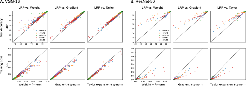
Figure 6: Performance comparison of the proposed method (i.e. LRP) and other criteria on VGG-16 and ResNet-50 with five datasets. Each point in the scatter plot corresponds to the performance at a specific pruning rate of two criteria, where the vertical axis shows the performance of our LRP criterion and the horizontal axis the performance of a single other criterion (compare to Figure 5 that displays the same data for more than two criteria). The black dashed line shows the set of points where models pruned by one of the compared criteria would exhibit identical performance to LRP. For accuracy, higher values are better. For loss, lower values are better.

4.2.1 Scenario 1: Pruning with Fine-tuning

On the first scenario, we retrain the model after each iteration of pruning in order to regain lost performance. We then evaluate the performance of the different pruning criteria after each pruning-retraining-step.

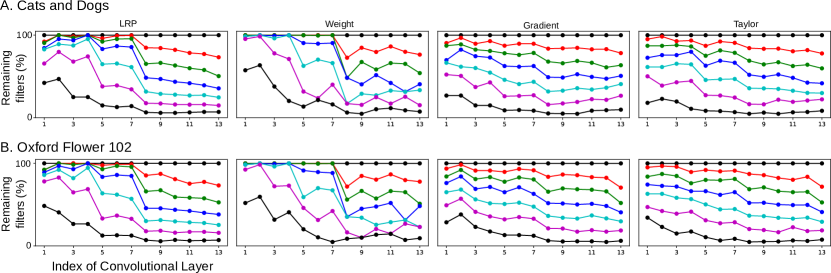
Figure 7: An observation of per-layer pruning performed w.r.t the different evaluated criteria on VGG-16 and two datasets. Each colored line corresponds to a specific (global) ratio of filters pruned from the network ( black (top) : 0%, red : 15%, green: 30%, blue: 45%, violet: 75% and black (bottom) 90%). The dots on each line identify the ratio of pruning applied to specific convolutional layers, given a global ratio of pruning, depending on the pruning criterion.

That is, we quantify the importance of each filter by the magnitude of the respective criterion and iteratively prune 5% of all filters (w.r.t. the original number of filters in the model) rated least important in each pruning step. Then, we compute and record the training loss, test accuracy, number of remaining parameters and total estimated FLOPs. We assume that the least important filters should have only little influence on the prediction and thus incur the lowest performance drop if they are removed from the network.

Figure 5 (and Supplementary Figure 2) depict test accuracies with increasing pruning rate in VGG-16 and ResNet-50 (and AlexNet and ResNet-18, respectively) after fine-tuning for each dataset and each criterion. It is observed that LRP achieves higher test accuracies compared to other criteria in a large majority of cases (see Figure 6 and Supplementary Figure 1). These results demonstrate that the performance of LRP-based pruning is stable and independent of the chosen dataset. Apart from performance, regularization by layer is a critical constraint which obstructs the expansion of some of the criteria toward several pruning strategies such as local pruning, global pruning, etc. Except for the LRP criterion, all criteria perform substantially worse without $l_{p}$ regularization compared to those with $l_{p}$ regularization and result in unexpected interruptions during the pruning process due to the biased redistribution of importance in the network (cf. top rows of Figure 5 and Supplementary Figure 2).

Table 3 shows the predictive performance of the different criteria in terms of training loss, test accuracy, number of remaining parameters and FLOPs , for the VGG-16 and ResNet-50 models. Similar results for AlexNet and ResNet-18 can be found in Supplementary Table 2. Except for CIFAR-10, the highest compression rate (i.e. lowest number of parameters) could be achieved by the proposed LRP-based criterion (row “Params”) for VGG-16, but not for ResNet-50. However, in terms of FLOPs, the proposed criterion only outperformed the weight criterion, but not the Taylor and Gradient criteria (row“FLOPs”). This is due to the fact that a reduction in number of FLOPs depends on the location where pruning is applied within the network: Figure 7 shows that the LRP and weight criteria focus the pruning on upper layers closer to the model output, whereas the Taylor and Gradient criteria focus more on the lower layers.

Throughout the pruning process usually a gradual decrease in performance can be observed. However, with the Event 8, Oxford Flower 102 and CIFAR-10 datasets, pruning leads to an initial performance increase, until a pruning rate of approx. 30% is reached. This behavior has been reported before in the literature and might stem from improvements of the model structure through elimination of filters related to classes in the source dataset (i.e., ILSVRC 2012) that are not present in the target dataset anymore [44]. Supplementary Table 3 and Supplementary Figure 2 similarly show that LRP achieves the highest test accuracy in AlexNet and ResNet-18 for nearly all pruning ratios with almost every dataset.

Figure 7 shows the number of the remaining convolutional filters for each iteration. We observe that, on the one hand, as pruning rate increases, the convolutional filters in earlier layers that are associated with very generic features, such as edge and blob detectors, tend to generally be preserved as opposed to those in latter layers which are associated with abstract, task-specific features. On the other hand, the LRP- and weight-criterion first keep the filters in early layers in the beginning, but later aggressively prune filters near the input which now have lost functionality as input to later layers, compared to the gradient-based criteria such as gradient and Taylor-based approaches. Although gradient-based criteria also adopt the greedy layer-by-layer approach, we can see that gradient-based criteria pruned the less important filters almost uniformly across all the layers due to re-normalization of the criterion in each iteration. However, this result contrasts with previous gradient-based works [22, 25] that have shown that units deemed unimportant in earlier layers, contribute significantly compared to units deemed important in latter layers. In contrast to this, LRP can efficiently preserve units in the early layers — as long as they serve a purpose — despite of iterative global pruning.

4.2.2 Scenario 2: Pruning without Fine-tuning

In this section, we evaluate whether pruning works well if only a (very) limited number of samples is available for quantifying the pruning criteria. To the best of our knowledge, there are no previous studies that show the performance of pruning approaches when acting w.r.t. very small amounts of data. With large amounts of data available (and even though we can expect reasonable performance after pruning), an iterative pruning and fine-tuning procedure of the network can amount to a very time consuming and computationally heavy process. From a practical point of view, this issue becomes a significant problem, e.g. with limited computational resources (mobile devices or in general; consumer-level hardware) and reference data (e.g., private photo collections), where capable and effective one-shot pruning approaches are desired and only little leeway (or none at all) for fine-tuning strategies after pruning is available.

To investigate whether pruning is possible also in these scenarios, we performed experiments with a relatively small number of data on the 1) Cats & Dogs and 2) subsets from the ILSVRC 2012 classes. On the Cats & Dogs dataset, we only used 10 samples each from the “cat” and “dog” classes to prune the (on ImageNet) pre-trained AlexNet, VGG-16, ResNet-18 and ResNet-50 networks with the goal of domain/dataset adaption. The binary classification (i.e. “cat” vs. “dog”) is a subtask within the ImageNet taxonomy and corresponding output neurons can be identified by its WordNet associations. This experiment implements the task of domain adaptation.

In a second experiment on the ILSVRC 2012 dataset, we randomly chose $k=3$ classes for the task of model specialization, selected only $n=10$ images per class from the training set and used them to compare the different pruning criteria. For each criterion, we used the same selection of classes and samples. In both experimental settings, we do not fine-tune the models after each pruning iteration, in contrast to Scenario 1 in Section 4.2.1. The obtained post-pruning model performance is averaged over 20 random selections of classes (ImageNet) and samples (Cats & Dogs) to account for randomness. Please note that before pruning, we first restructured the models’ fully connected output layers to only preserve the task-relevant $k$ network outputs by eliminating the $1000-k$ redundant output neurons.

Furthermore, as our target datasets are relatively small and only have an extremely reduced set of target classes, the pruned models could still be very heavy w.r.t. memory requirements if the pruning process would be limited to the convolutional layers, as in Section 4.2.1. More specifically, while convolutional layers dominantly constitute the source of computation cost (FLOPs), fully connected layers are proven to be more redundant [29]. In this respect, we applied pruning procedures in both fully connected layers and convolutional layers in combination for VGG-16.

For pruning, we iterate a sequence of first pruning filters from the convolutional layers, followed by a step of pruning neurons from the model’s fully connected layers. Note that both evaluated ResNet architectures mainly consist of convolutional- and pooling layers, and conclude in a single dense layer, of which the set of input neurons are only affected via their inputs by pruning the below convolutional stack. We therefore restrict the iterative pruning filters from the sequence of dense layers of the feed-forward architecture of the VGG-16.

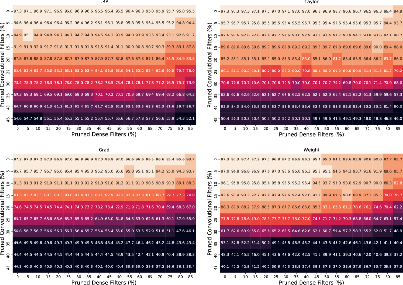
Figure 8: Test accuracy after pruning of $n\%$ of convolutional (rows) and $m\%$ of fully connected (columns) filters on VGG-16 without fine-tuning for a random subset of the classes from ILSVRC 2012 ($k$ = 3) based on different criteria (averaged over 20 repetitions). Each color represents a range of 5% in test accuracy. The brighter the color the better the performance after a given degree of pruning .

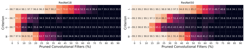
Figure 9: Test accuracy after pruning of $n\%$ of convolutional filters on ResNet18 and ResNet50 without fine-tuning for a random subset of the classes from ILSVRC 2012 ($k$ = 3) based on the criteria Weight, Taylor, Gradient with $\ell_{2}$-norm and LRP (averaged over 20 repetitions). Compare to Figure 8 .

The model performance after the application of each criterion for classifying a small number of classes ($k$ = 3) from the ILSVRC 2012 dataset is indicated in Figure 8 for VGG 16 and Figure 9 for ResNets (please note again that ResNets do not have fully-connected layers). During pruning at fully-connected layers, no significant difference across different pruning ratios can be observed. Without further fine-tuning, pruning weights/filters at the fully connected layers can retain performance efficiently. However, there is a certain difference between LRP and other criteria with increasing pruning ratio of convolutional layers for VGG-16/ResNet-18/ResNet-50, respectively: (LRP vs. Taylor with $l_{2}$-norm; up to of 9.6/61.8/51.8%, LRP vs. gradient with $l_{2}$-norm; up to 28.0/63.6/54.5 %, LRP vs. weight with $l_{2}$-norm; up to 27.1/48.3/30.2 %). Moreover, pruning convolutional layers needs to be carefully managed compared to pruning fully connected layers. We can observe that LRP is applicable for pruning any layer type (i.e. fully connected, convolutional, pooling, etc.) efficiently. Additionally, as mentioned in Section 3.1, our method can be applied to general network architectures because it can automatically measure the importance of weights or filters in a global (network-wise) context without further normalization.

Figure 10 shows the test accuracy as a function of the pruning ratio, in context a domain adaption task from ImageNet towards the Cats & Dogs dataset for all models. As the pruning ratio increases, we can see that even without fine-tuning, using LRP as pruning criterion can keep the test accuracy not only stable, but close to 100%, given the extreme scarcity of data in this experiment. In contrast, the performance decreases significantly when using the other criteria requiring an application of the $l_{2}$-norm. Initially, the performance is even slightly increasing when pruning with LRP. During iterative pruning, unexpected changes in accuracy with LRP (for 2 out of 20 repetitions of the experiment) have been shown around 50 - 55% pruning ratio, but accuracy is regained quickly again. However, only the VGG-16 model seems to be affected, and none other for this task. For both ResNet models, this phenomenon occurs for the other criteria instead. A series of in-depth investigations of this momentary decrease in performance did not lead to any insights and will be subject of future work.

By pruning over 99% of convolutional filters in the networks using our proposed method, we can have 1) greatly reduced computational cost, 2) faster forward and backward processing (e.g. for the purpose of further training, inference or the computation of attribution maps), and 3) a lighter model even in the small sample case, all while adapting off-the-shelf pre-trained ImageNet models towards a dog-vs.-cat classification task.

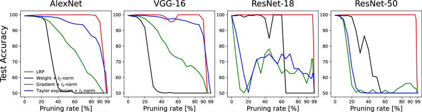
Figure 10: Performance comparison of pruning without fine-tuning for AlexNet, VGG-16, ResNet-18 and ResNet-50 based on only few (10) samples per class from the Cats & Dogs dataset, as a means for domain adaption. Additional results on further target domains can be found in the Supplement with Supplementary Figure 3.

5 Discussion

Our experiments demonstrate that the novel LRP criterion consistently performed well compared to other criteria across various datasets, model architectures and experimental settings, and oftentimes outperformed the competing criteria. This is especially pronounced in our Scenario 2 (cf. Section 4.2.2), where only little resources are available for criterion computation, and no fine-tuning after pruning is allowed. Here, LRP considerably outperformed the other metrics on toy data (cf. Section 4.1) and image processing benchmark data (cf. Section 4.2.2). The strongly similar results between criteria observed in Scenario 1 (cf. Section 4.2.2) are also not surprising, as an additional file-tuning step after pruning may allow the pruned neural network model to recover its original performance, as long as the model has the capacity to do so [22].

From the results of Table 3 and Supplementary Table 3 we can observe that with a fixed pruning target of $n\%$ filters removed, LRP might not always result in the cheapest sub-network after pruning in terms of parameter count and FLOPs per inference, however it consistently is able to identify the network components for removal and preservation leading to the best performing model after pruning. Latter results resonate also strongly in our experiments of Scenario 2 on both image and toy data, where, without the additional fine-tuning step, the LRP-pruned models vastly outperform their competitors. The results obtained in multiple toy settings verify that only the LRP-based pruning criterion is able to preserve the original structure of the prediction function (cf. Figures 2 and 3).

Unlike the weight criterion, which is a static quantity once the network is not in training anymore, the criteria Taylor, gradient and LRP require reference samples for computation, which in turn may affect the estimation of neuron importance. From the latter three criteria, however, only LRP provides a continuous measure of network structure importance (cf. Sec 7.2 in [12]) which does not suffer from abrupt changes in the estimated importance measures with only marginal steps between reference samples. This quality of continuity is reflected in the stability and quality of LRP results reported in Section 4.1, compared to the high volatility in neuron selection for pruning and model performance after pruning observable for the gradient and Taylor criteria. From this observation it can also be deduced that LRP requires relatively few data points to converge to a pruning solution that possesses a similar prediction behavior as the original model. Hence, we conclude that LRP is a robust pruning criterion that is broadly applicable in practice. Especially in a scenario where no finetuning is applied after pruning (see Sec. 4.2.2), the LRP criterion allows for pruning of a large part of the model without significant accuracy drops.

In terms of computational cost, LRP is comparable to the Taylor and Gradient criteria because these criteria require both a forward and a backward pass for all reference samples. The weight criterion is substantially cheaper to compute since it does not require to evaluate any reference samples; however, its performance falls short in most of our experiments. Additionally, our experiments demonstrate that LRP requires less reference samples than the other criteria (cf. Figure 3 and Figure 4), thus the required computational cost is lower in practical scenarios, and better performance can be expected if only low numbers of reference samples are available (cf. Figure 10).

Unlike all other criteria, LRP does not require explicit regularization via $\ell_{p}$-normalization, as it is naturally normalized via its enforced relevance conservation principle during relevance backpropagation, which leads to the preservation of important network substructures and bottlenecks in a global model context. In line with the findings by [22], our results in Figure 5 and Supplementary Figure 2 show that additional normalization after criterion computation for weight, gradient and Taylor is not only vital to obtain good performance, but also to avoid disconnected model segments — something which is prevented out-of-the-box with LRP.

However, our proposed criterion still provides several open questions that deserve a deeper investigation in future work. First of all, LRP is not implementation invariant, i.e., the structure and composition of the analyzed network might affect the computation of the LRP-criterion and “network canonization” — a functionally equivalent restructuring of the model — might be required for optimal results, as discussed early in Section 4 and [43]. Furthermore, while our LRP-criterion does not require additional hyperparameters, e.g., for normalization, the pruning result might still depend on the chosen LRP variant. In this paper, we chose the $\alpha_{1}\beta_{0}$-rule in all layers, because this particular parameterization identifies the network’s neural pathways positively contributing to the selected output neurons for which reference samples are provided, is robust to the detrimental effects of shattered gradients affecting especially very deep CNNs [11] (i.e., other than gradient-based methods, it does not suffer from potential discontinuities in the backpropagated quantities), and has a mathematical well-motivated foundation in DTD [11, 12]. However, other work from literature provide [14] or suggest [9, 8] alternative parameterizations to optimize the method for explanatory purposes. It is an interesting direction for future work to examine whether these findings also apply to LRP as a pruning criterion.

6 Conclusion

Modern CNNs typically have a high capacity with millions of parameters as this allows to obtain good optimization results in the training process. After training, however, high inference costs remain, despite the fact that the number of effective parameters in the deep model is actually significantly lower (see e.g. [45]). To alleviate this, pruning aims at compressing and accelerating the given models without sacrificing much predictive performance. In this paper, we have proposed a novel criterion for the iterative pruning of CNNs based on the explanation method LRP, linking for the first time two so far disconnected lines of research. LRP has a clearly defined meaning, namely the contribution of an individual network unit, i.e. weight or filter, to the network output. Removing units according to low LRP scores thus means discarding all aspects in the model that do not contribute relevance to its decision making. Hence, as a criterion, the computed relevance scores can easily and cheaply give efficient compression rates without further postprocessing, such as per-layer normalization. Besides, technically LRP is scalable to general network structures and its computational cost is similar to the one of a gradient backward pass.

In our experiments, the LRP criterion has shown favorable compression performance on a variety of datasets both with and without retraining after pruning. Especially when pruning without retraining, our results for small datasets suggest that the LRP criterion outperforms the state of the art and therefore, its application is especially recommended in transfer learning settings where only a small target dataset is available.

In addition to pruning, the same method can be used to visually interpret the model and explain individual decisions as intuitive relevance heatmaps. Therefore, in future work, we propose to use these heatmaps to elucidate and explain which image features are most strongly affected by pruning to additionally avoid that the pruning process leads to undesired Clever Hans phenomena [8].

Pruning by Explaining: A Novel Criterion for
Deep Neural Network Pruning
— Supplementary Materials —

Supplementary Methods 1: Data Preprocessing

During fine-tuning, images are resized to 256$\times$256 and randomly cropped to 224$\times$224 pixels, and then horizontally flipped with a random chance of 50% for data augmentation. For testing, images are resized to 224$\times$224 pixels.

Scene 15: The Scene 15 dataset contains about 4,485 images and consists of 15 natural scene categories obtained from COREL collection, Google image search and personal photographs [36]. We fine-tuned four different models on 20% of the images from each class and achieved initial Top-1 accuracy of 88.59% for VGG-16, 85.48% for AlexNet, 83.96% for ResNet-18, and 88.28% for ResNet-50, respectively.

Event 8: Event-8 consists of 8 sports event categories by integrating scene and object recognition. We use 40% of the dataset’s images for fine-tuning and the remaining 60% for testing. We adopted the common data augmentation method as in [26].

Cats and Dogs: This is the Asirra dataset provided by Microsoft Research (from Kaggle). The given dataset for the competition (KMLC-Challenge-1) [38]. Training dataset contains 4,000 colored images of dogs and 4,005 colored images of cats, while containing 2,023 test images. We reached initial accuracies of 99.36% for VGG-16, 96.84% for AlexNet, 97.97% for ResNet-18, and 98.42% for ResNet-50 based on transfer learning approach.

Oxford Flowers 102: The Oxford Flowers 102 dataset contains 102 species of flower categories found in the UK, which is a collection with over 2,000 training and 6,100 test images [39]. We fine-tuned models with pre-trained networks on ImageNet for transfer learning.

CIFAR-10: This dataset contains 50,000 training images and 10,000 test images spanning 10 categories of objects. The resolution of each image is 32$\times$32 pixels and therefore we resize the images as 224$\times$224 pixels.

ILSVRC 2012: In order to show the effectiveness of the pruning criteria in the small sample scenario, we pruned and tested all models on randomly selected $k=3$ from 1000 classes and data from the ImageNet corpus [40].

Supplementary Results 1: Additional results on toy data

Supplementary Table 1: Comparison of training accuracy after one-shot pruning one third of all filters w.r.t one of the four metrics on toy datasets, with $n\in[1,5,20,100]$ reference samples used for criteria computation for Weight, Gradient, Taylor and LRP. Compare to Figure 4.

Dataset	Unpruned	Pruned
			n=1			n=5			n=20			n=100
		W	T	G	L	T	G	L	T	G	L	T	G	L
moon	99.90	99.60	79.80	83.07	85.01	84.70	86.07	99.86	86.99	85.87	99.85	94.77	93.53	99.85
circle	100.00	97.10	68.35	69.21	70.23	87.18	82.23	99.89	91.87	85.36	100.00	97.04	90.88	100.00
multi	94.95	91.00	34.28	34.28	62.98	77.34	67.96	91.85	83.21	77.39	91.59	84.76	82.68	91.25

Here, we discuss with Supplementary Table 2 the consistency of LRP-based neuron selection across reference sample sizes. One can assume that the larger the choice of $n$ the less volatile is the choice of (un)important neurons by the criterion, as the influence of individual reference samples is marginalized out. We therefore compare the first and last ranked sets of neurons selected for a low (yet due to our observations sufficient) number $n=10$ of reference samples to all other reference sample set sizes $m$ over all unique random seed combinations. For all comparisons of $n\times m$ (except for $m=1$) we observe a remarkable consistency in the selection of (un)important network substructures. With an increasing $m$, we can see the consistency in neuron set selection gradually increase and then plateau for the “moon” and “circle” datasets, which means that the selected set of neurons remains consistent for larger sets of reference samples from that point on. For the “mult” toy dataset, we observe a gradual yet minimal decrease in the set similarity scores for $m\geq 10$, which means that the results deviate from the selected neurons for $n=10$, i.e. variability over the neuron sets selected for $n=10$ are the source of the volatility between $n$-reference and $m$-reference selected neuron sets. In all cases, peak consistency is achieved at $n\in\{5,10\}$ reference samples, identifying low numbers of $n\in\{5,10\}$ as sufficient for consistently pruning our toy models.

Supplementary Table 2: A consistency comparison of neuron selection of LRP between reference sample sets sized $n$, averaged over all 1225 unique random seed combinations. Higher values indicate higher consistency. We report results for $n=10$ reference samples in comparison to $m\in[1,{2,}5,10,20,50,100,200]$ reference samples per class and $k=250$. Observations for all other combinations of $n\times m$, $k\in[125,500,1000]$ and all other criteria are available on github³.

Dataset	$n$		first-250								last-250
		$m=$	$1$	$2$	$5$	$10$	$20$	$50$	$100$	$200$	$1$	$2$	$5$	$10$	$20$	$50$	$100$	$200$
moon	$10$		0.687	0.865	0.942	0.947	0.951	0.952	0.950	0.950	0.676	0.810	0.916	0.928	0.938	0.946	0.947	0.948
circle	$10$		0.689	0.795	0.831	0.843	0.845	0.846	0.846	0.842	0.698	0.874	0.919	0.937	0.946	0.951	0.953	0.954
mult	$10$		0.142	0.625	0.773	0.791	0.779	0.765	0.763	0.762	0.160	0.697	0.890	0.942	0.940	0.936	0.934	0.933

Supplementary Results 2: Additional results for image processing neural networks

Here, we provide results for AlexNet and ResNet-18 — in addition to the VGG16 and ResNet-50 results shown in the main paper — in Supplementary Figure 1 (cf. Figure 6), Supplementary Figure 2 (cf. Figure 5), and Supplementary Table 3 (cf. Table 3). These results demonstrate that the favorable pruning performance of our LRP criterion is not limited to any specific network architecture. We remark that the results for CIFAR-10 show a larger robustness to higher pruning rates. This is due to the fact that CIFAR-10 has the lowest resolution as dataset and little structure in its images as a consequence. The images contain components with predominantly very low frequencies. The filters, which are covering higher frequencies, are expected to be mostly idle for CIFAR-10. This makes the pruning task less challenging. Therefore no method can clearly distinguish itself by a different pruning strategy which addresses those filters which are covering the higher frequencies in images.

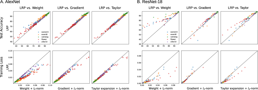
Supplementary Figure 1: Performance comparison of the proposed method (i.e. LRP) and other criteria on AlexNet and ResNet-18 with five datasets. Each point in the scatter plot corresponds to the performance at a specific pruning rate of two criteria, where the vertical axis shows the performance of LRP and the horizontal axis the performance of one other criterion (compare to Supplementary Figure 2 that displays the same data for more than two criteria). The black dashed line shows the set of points where models pruned by one of the compared criteria would exhibit identical performance to LRP. For accuracy, higher values are better. For loss, lower values are better. Compare to Figure 6.

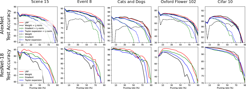
Supplementary Figure 2: Comparison of test accuracy in different criteria as pruning rate increases on AlexNet (top) and ResNet-18 (bottom) with five datasets. Pruning with fine-tuning. Prematurely terminated lines indicate that during pruning, the respective criterion removed vital filters and thus disconnected the model input from the output. Compare to Figure 5.

Supplementary Table 3: A performance comparison between criteria (Weight, Taylor, Gradient with $\ell_{2}$-norm and LRP) and the Unpruned model for AlexNet (top) and ResNet-18 (bottom) on five different image benchmark datasets. Criteria are evaluated at fixed pruning rates per model and dataset, identified as $\langle$dataset$\rangle$@$\langle$percent_pruned_filters$\rangle$%. We report test accuracy (in %), (training) loss ($\times 10^{-2}$), number of remaining parameters ($\times 10^{7})$ and FLOPs (in MMACS for AlexNet and GMACS for ResNet-18) per forward pass. For all measures except accuracy, lower outcomes are better. Compare to Table 3.

AlexNet	Scene 15 @ 55%					Event 8 @ 55%					Cats & Dogs @ 60%
	U	W	T	G	L	U	W	T	G	L	U	W	T	G	L
Loss	2.49	2.78	2.31	2.46	2.02	1.16	1.67	1.21	1.37	1.00	0.50	0.77	0.78	0.87	0.70
Accuracy	85.48	78.43	79.40	78.63	80.76	94.89	88.10	88.62	88.42	90.41	96.84	95.86	95.23	94.89	95.81
Params	54.60	35.19	33.79	33.29	33.93	54.57	34.25	33.00	33.29	32.79	54.54	32.73	33.50	33.97	32.66
FLOPs	711.51	304.88	229.95	225.19	277.98	711.48	301.9	241.18	238.36	291.95	711.46	264.04	199.88	190.84	240.19
	Oxford Flower 102 @ 70%					CIFAR-10 @ 30%
	U	W	T	G	L	U	W	T	G	L
Loss	5.15	4.83	3.39	3.77	3.01	1.95	2.44	2.46	2.46	2.33
Accuracy	78.74	63.93	64.10	64.11	65.69	87.83	90.03	89.48	89.58	89.87
Params	54.95	28.13	29.19	28.72	28.91	54.58	48.31	84.23	46.31	48.22
FLOPs	711.87	192.69	132.34	141.82	161.35	711.49	477.16	371.48	395.43	402.93
ResNet-18	Scene 15 @ 50%					Event 8 @ 55%					Cats & Dogs @ 45%
	U	W	T	G	L	U	W	T	G	L	U	W	T	G	L
Loss	1.32	1.98	1.28	1.03	0.85	0.61	1.28	0.99	0.72	0.55	0.03	0.04	0.05	0.04	0.02
Accuracy	83.97	69.95	78.14	78.24	81.61	95.63	80.20	83.81	86.76	90.27	97.97	97.17	96.34	94.13	97.91
Params	11.18	4.63	4.91	4.96	4.52	11.18	3.99	4.17	4.26	3.89	11.18	4.88	5.18	5.15	5.04
FLOPs	1.82	1.30	1.16	1.10	1.27	1.82	1.22	1.11	1.07	1.20	1.82	1.36	1.22	1.21	1.36
	Oxford Flower 102 @ 70%					CIFAR-10 @ 30%
	U	W	T	G	L	U	W	T	G	L
Loss	1.36	4.64	2.96	1.65	1.59	0.000	0.002	0.012	0.016	0.004
Accuracy	71.23	34.58	49.56	62.41	65.60	94.67	94.21	92.71	92.55	94.03
Params	11.23	2.19	3.07	3.07	2.45	11.17	6.88	7.85	7.56	6.62
FLOPs	1.82	0.95	0.72	0.73	0.93	0.56	0.46	0.42	0.41	0.47

Furthermore, the ASSIRA dataset of cats and dogs may raise the concern that it is the MNIST analogue for pets, representing a rather simple problem, and for that reason the results might not be transferable to problems with larger variance. To validate our observation, we have chosen the more lightweight [46] ResNet-50 model, and evaluated its pruning performance on three further datasets. Each of the three datasets is composed as a binary discrimination problem obtained by fusing two datasets chosen from the following selection: FGVC aircraft [47], CUB birds [48] and Stanford cars [49]. We have chosen these three datasets, as they are known from the literature, have an intrinsic variability as visible by their numbers of classes and a medium sample size. Most importantly, we know for these datasets that the object categories defining their contents are matched by some classes in the ImageNet dataset which is used to initialize the weights of the ResNet-50 network.

Supplementary Figure 3 shows the results for the three composed discrimination problems, without fine-tuning after pruning. We can observe that each pruning method is able to remove a certain amount of network filters without notable loss of discrimination performance. Weight-based pruning performs second best, while LRP-based pruning allows consistently to prune the largest fraction of filters before starting to lose prediction accuracy.

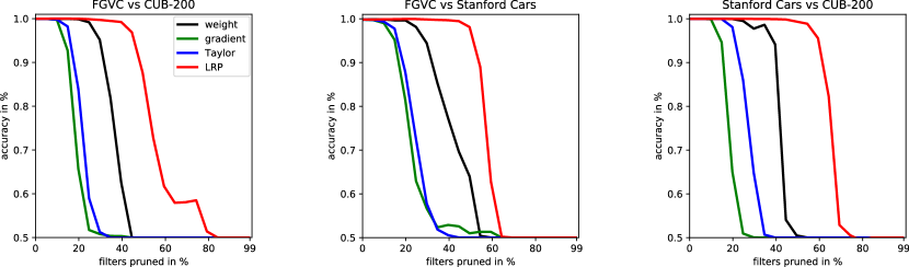
Supplementary Figure 3: Comparison of pruning performance without a subsequent finetuning step for a ResNet-50 network when pruned by criteria using weights, gradient, Taylor-expansion and LRP. Each dataset is a binary classification problem created by combining two datasets taken from FGVC Aircraft [47], CUB-200-2011 birds [48] and Stanford Cars [49], which are covered by similar classes in the ImageNet initialization. Results are the average of 20 repetitions with randomly drawn samples. Each run relies on 20 samples for pruning, 10 from each of the two datasets, and 2048 samples for test accuracy evaluation. For a given repetition, all methods use the same set of samples for pruning and they use a set of samples for evaluation, which is again identical for all pruning methods, but disjoint from the pruning set. Compare to Figure 10.

When comparing cats versus dogs in Figure 10 against the three composed datasets in Supplementary Figure 3, we observe that there is less redundant capacity which can be pruned away for the composed datasets. This sanity check is in line with the higher variance of these composed datasets as compared to cats versus dogs. As a side remark, this observation suggests the thought to measure empirically dataset complexities with respect to a neural network by the area under the accuracy graph with respect to the amount of pruned filters.

References

- Gu et al. [2018] J. Gu, Z. Wang, J. Kuen, L. Ma, A. Shahroudy, B. Shuai, T. Liu, X. Wang, G. Wang, J. Cai, T. Chen, Recent advances in convolutional neural networks, Pattern Recognition 77 (2018) 354–377.
- Denil et al. [2013] M. Denil, B. Shakibi, L. Dinh, M. Ranzato, N. de Freitas, Predicting parameters in deep learning, in: Advances in Neural Information Processing Systems (NIPS), 2013, pp. 2148–2156.
- Sze et al. [2017] V. Sze, Y. Chen, T. Yang, J. S. Emer, Efficient processing of deep neural networks: A tutorial and survey, Proceedings of the IEEE 105 (2017) 2295–2329.
- LeCun et al. [1989] Y. LeCun, J. S. Denker, S. A. Solla, Optimal brain damage, in: Advances in Neural Information Processing Systems (NIPS), 1989, pp. 598–605.
- Tu and Lin [2019] Y. Tu, Y. Lin, Deep neural network compression technique towards efficient digital signal modulation recognition in edge device, IEEE Access 7 (2019) 58113–58119.
- Cheng et al. [2018] Y. Cheng, D. Wang, P. Zhou, T. Zhang, Model compression and acceleration for deep neural networks: The principles, progress, and challenges, IEEE Signal Processing Magazine 35 (2018) 126–136.
- Bach et al. [2015] S. Bach, A. Binder, G. Montavon, F. Klauschen, K.-R. Müller, W. Samek, On pixel-wise explanations for non-linear classifier decisions by layer-wise relevance propagation, PLoS ONE 10 (2015) e0130140.
- Lapuschkin et al. [2019] S. Lapuschkin, S. Wäldchen, A. Binder, G. Montavon, W. Samek, K.-R. Müller, Unmasking Clever Hans predictors and assessing what machines really learn, Nature Communications 10 (2019) 1096.
- Hägele et al. [2020] M. Hägele, P. Seegerer, S. Lapuschkin, M. Bockmayr, W. Samek, F. Klauschen, K.-R. Müller, A. Binder, Resolving challenges in deep learning-based analyses of histopathological images using explanation methods, Scientific Reports 10 (2020) 6423.
- Seegerer et al. [2020] P. Seegerer, A. Binder, R. Saitenmacher, M. Bockmayr, M. Alber, P. Jurmeister, F. Klauschen, K.-R. Müller, Interpretable deep neural network to predict estrogen receptor status from haematoxylin-eosin images, in: Artificial Intelligence and Machine Learning for Digital Pathology: State-of-the-Art and Future Challenges, Springer International Publishing, Cham, 2020, pp. 16–37.
- Montavon et al. [2017] G. Montavon, S. Lapuschkin, A. Binder, W. Samek, K.-R. Müller, Explaining nonlinear classification decisions with deep taylor decomposition, Pattern Recognition 65 (2017) 211–222.
- Montavon et al. [2018] G. Montavon, W. Samek, K.-R. Müller, Methods for interpreting and understanding deep neural networks, Digital Signal Processing 73 (2018) 1–15.
- Samek et al. [2020] W. Samek, G. Montavon, S. Lapuschkin, C. J. Anders, K.-R. Müller, Toward interpretable machine learning: Transparent deep neural networks and beyond, arXiv preprint arXiv:2003.07631 (2020).
- Alber et al. [2019] M. Alber, S. Lapuschkin, P. Seegerer, M. Hägele, K. T. Schütt, G. Montavon, W. Samek, K.-R. Müller, S. Dähne, P.-J. Kindermans, iNNvestigate neural networks!, Journal of Machine Learning Research 20 (2019) 93:1–93:8.
- Wiedemann et al. [2020] S. Wiedemann, K.-R. Müller, W. Samek, Compact and computationally efficient representation of deep neural networks, IEEE Transactions on Neural Networks and Learning Systems 31 (2020) 772–785.
- Tung and Mori [2020] F. Tung, G. Mori, Deep neural network compression by in-parallel pruning-quantization, IEEE Transactions on Pattern Analysis and Machine Intelligence 42 (2020) 568–579.
- Guo et al. [2019] K. Guo, X. Xie, X. Xu, X. Xing, Compressing by learning in a low-rank and sparse decomposition form, IEEE Access 7 (2019) 150823–150832.
- Xu et al. [2019] T. Xu, P. Yang, X. Zhang, C. Liu, LightweightNet: Toward fast and lightweight convolutional neural networks via architecture distillation, Pattern Recognition 88 (2019) 272–284.
- Zhang et al. [2018] X. Zhang, X. Zhou, M. Lin, J. Sun, Shufflenet: An extremely efficient convolutional neural network for mobile devices, in: IEEE Conference on Computer Vision and Pattern Recognition (CVPR), 2018, pp. 6848–6856.
- Molchanov et al. [2019] P. Molchanov, A. Mallya, S. Tyree, I. Frosio, J. Kautz, Importance estimation for neural network pruning, in: IEEE Conference on Computer Vision and Pattern Recognition (CVPR), 2019, pp. 11264–11272.
- Hassibi and Stork [1992] B. Hassibi, D. G. Stork, Second order derivatives for network pruning: Optimal brain surgeon, in: Advances in Neural Information Processing Systems (NIPS), 1992, pp. 164–171.
- Molchanov et al. [2017] P. Molchanov, S. Tyree, T. Karras, T. Aila, J. Kautz, Pruning convolutional neural networks for resource efficient transfer learning, in: Proceedings of the International Conference on Learning Representations (ICLR), 2017.
- Yu et al. [2019] C. Yu, J. Wang, Y. Chen, X. Qin, Transfer channel pruning for compressing deep domain adaptation models, International Journal of Machine Learning and Cybernetics 10 (2019) 3129–3144.
- Liu and Wu [2019] C. Liu, H. Wu, Channel pruning based on mean gradient for accelerating convolutional neural networks, Signal Processing 156 (2019) 84–91.
- Sun et al. [2017] X. Sun, X. Ren, S. Ma, H. Wang, meprop: Sparsified back propagation for accelerated deep learning with reduced overfitting, in: International Conference on Machine Learning (ICML), 2017, pp. 3299–3308.
- Han et al. [2015] S. Han, J. Pool, J. Tran, W. J. Dally, Learning both weights and connections for efficient neural network, in: Advances in Neural Information Processing Systems (NIPS), 2015, pp. 1135–1143.
- Han et al. [2016] S. Han, X. Liu, H. Mao, J. Pu, A. Pedram, M. A. Horowitz, W. J. Dally, EIE: efficient inference engine on compressed deep neural network, in: International Symposium on Computer Architecture (ISCA), 2016, pp. 243–254.
- Wen et al. [2016] W. Wen, C. Wu, Y. Wang, Y. Chen, H. Li, Learning structured sparsity in deep neural networks, in: Advances in Neural Information Processing Systems (NIPS), 2016, pp. 2074–2082.
- Li et al. [2017] H. Li, A. Kadav, I. Durdanovic, H. Samet, H. P. Graf, Pruning filters for efficient convnets, in: International Conference on Learning Representations, (ICLR), 2017.
- Yu et al. [2018] R. Yu, A. Li, C. Chen, J. Lai, V. I. Morariu, X. Han, M. Gao, C. Lin, L. S. Davis, NISP: pruning networks using neuron importance score propagation, in: IEEE Conference on Computer Vision and Pattern Recognition (CVPR), 2018, pp. 9194–9203.
- Luo et al. [2019] J.-H. Luo, H. Zhang, H.-Y. Zhou, C.-W. Xie, J. Wu, W. Lin, ThiNet: Pruning CNN filters for a thinner net, IEEE Transactions on Pattern Analysis and Machine Intelligence 41 (2019) 2525–2538.
- Gan et al. [2020] J. Gan, W. Wang, K. Lu, Compressing the CNN architecture for in-air handwritten Chinese character recognition, Pattern Recognition Letters 129 (2020) 190 – 197.
- Dai et al. [2019] X. Dai, H. Yin, N. K. Jha, Nest: A neural network synthesis tool based on a grow-and-prune paradigm, IEEE Transactions on Computers 68 (2019) 1487–1497.
- Samek et al. [2019] W. Samek, G. Montavon, A. Vedaldi, L. K. Hansen, K.-R. Müller (Eds.), Explainable AI: Interpreting, Explaining and Visualizing Deep Learning, volume 11700 of Lecture Notes in Computer Science, Springer, 2019.
- Samek et al. [2017] W. Samek, A. Binder, G. Montavon, S. Lapuschkin, K.-R. Müller, Evaluating the visualization of what a deep neural network has learned, IEEE Transactions on Neural Networks and Learning Systems 28 (2017) 2660–2673.
- Lazebnik et al. [2006] S. Lazebnik, C. Schmid, J. Ponce, Beyond bags of features: Spatial pyramid matching for recognizing natural scene categories, in: IEEE Conference on Computer Vision and Pattern Recognition (CVPR), 2006, pp. 2169–2178.
- Li and Li [2007] L. Li, F. Li, What, where and who? Classifying events by scene and object recognition, in: IEEE International Conference on Computer Vision (ICCV), 2007, pp. 1–8.
- Elson et al. [2007] J. Elson, J. R. Douceur, J. Howell, J. Saul, Asirra: a CAPTCHA that exploits interest-aligned manual image categorization, in: Proceedings of the 2007 ACM Conference on Computer and Communications Security (CCS), 2007, pp. 366–374.
- Nilsback and Zisserman [2008] M. Nilsback, A. Zisserman, Automated flower classification over a large number of classes, in: Sixth Indian Conference on Computer Vision, Graphics & Image Processing (ICVGIP), 2008, pp. 722–729.
- Russakovsky et al. [2015] O. Russakovsky, J. Deng, H. Su, J. Krause, S. Satheesh, S. Ma, Z. Huang, A. Karpathy, A. Khosla, M. S. Bernstein, A. C. Berg, F. Li, Imagenet large scale visual recognition challenge, International Journal of Computer Vision 115 (2015) 211–252.
- He et al. [2016] K. He, X. Zhang, S. Ren, J. Sun, Deep residual learning for image recognition, in: 2016 IEEE Conference on Computer Vision and Pattern Recognition, CVPR 2016, Las Vegas, NV, USA, June 27-30, 2016, 2016, pp. 770–778.
- Wang et al. [2018] H. Wang, Q. Zhang, Y. Wang, H. Hu, Structured probabilistic pruning for convolutional neural network acceleration, in: British Machine Vision Conference (BMVC), 2018, p. 149.
- Guillemot et al. [2020] M. Guillemot, C. Heusele, R. Korichi, S. Schnebert, L. Chen, Breaking batch normalization for better explainability of deep neural networks through layer-wise relevance propagation, CoRR abs/2002.11018 (2020).
- Liu et al. [2017] J. Liu, Y. Wang, Y. Qiao, Sparse deep transfer learning for convolutional neural network, in: AAAI Conference on Artificial Intelligence, 2017, pp. 2245–2251.
- Murata et al. [1994] N. Murata, S. Yoshizawa, S. Amari, Network information criterion-determining the number of hidden units for an artificial neural network model, IEEE Transactions on Neural Networks 5 (1994) 865–872.
- Bianco et al. [2018] S. Bianco, R. Cadene, L. Celona, P. Napoletano, Benchmark analysis of representative deep neural network architectures, IEEE Access 6 (2018) 64270–64277.
- Maji et al. [2013] S. Maji, E. Rahtu, J. Kannala, M. B. Blaschko, A. Vedaldi, Fine-Grained Visual Classification of Aircraft, Technical Report, 2013.
- Wah et al. [2011] C. Wah, S. Branson, P. Welinder, P. Perona, S. Belongie, The Caltech-UCSD Birds-200-2011 Dataset, Technical Report CNS-TR-2011-001, California Institute of Technology, 2011.
- Krause et al. [2013] J. Krause, M. Stark, J. Deng, L. Fei-Fei, 3d object representations for fine-grained categorization, in: 4th International IEEE Workshop on 3D Representation and Recognition (3dRR-13), Sydney, Australia, 2013.