General parametrization of Majorana neutrino mass models
One formula to fit them all!

Abstract

We discuss a general formula which allows to automatically reproduce experimental data for Majorana neutrino mass models, while keeping the complete set of the remaining model parameters free for general scans, as necessary in order to provide reliable predictions for observables outside the neutrino sector. We provide a proof of this master parametrization and show how to apply it for several well-known neutrino mass models from the literature. We also discuss a list of special cases, in which the Yukawa couplings have to fulfill some particular additional conditions.

I Introduction

Most of the classical Majorana neutrino mass models, such as the three tree-level seesaws (type-I Minkowski:1977sc ; Yanagida:1979as ; Mohapatra:1979ia ; GellMann:1980vs ; Schechter:1980gr , type-II Mohapatra:1980yp ; Schechter:1980gr and type-III Foot:1988aq ) or the 1-loop Zee model Zee:1980ai and the 2-loop Babu-Zee model Cheng:1980qt ; Zee:1985id ; Babu:1988ki have all been discussed already in the 1980’s. However, ever since the discovery of neutrino oscillations Fukuda:1998mi ; Ahmad:2002jz a miryad more of other neutrino mass models has been proposed in the literature.

To name a few papers and reviews post-1998, we mention Ma:1998dn , which showed that there are only three types of seesaws at tree-level. For a systematic analysis of all possible 1-loop diagrams, see Bonnet:2012kz . At 2-loop level we mention two different colored versions of the Babu-Zee topology Babu:2011vb ; Angel:2013hla . A general decomposition for all 2-loop models was presented in Sierra:2014rxa . At three-loop order there are the KNT Krauss:2002px , AKS Aoki:2008av and cocktail models Gustafsson:2012vj . And, recently, for 3-loops a systematic analysis was given in Cepedello:2018rfh . One can find even some examples of 4-loop models in the literature Gu:2011ak ; Helo:2015fba . For a recent review on radiative neutrino mass models, we refer to Cai:2017jrq .

One of the basic problems faced by model builders is to first reproduce correctly the measured neutrino masses and angles and to then scan over all remaining free parameters of the model in a systematic way, in order to explore possible predictions the model may make for other observables, such as $\mu\to e\gamma$ or neutrinoless double beta decay. It is often not difficult to identify some singular point in the parameter space of a given model, which explains oscillation data. However, exploring the parameter space in a complete and un-biased way seems not to be straight-foward in many cases. Here, we discuss in detail the master formula for neutrino mass models, introduced first in Cordero-Carrion:2018xre . All Majorana neutrino mass models can be brought to this form. We then discuss the master parametrization, a specific set of equations which allow to solve the above problem in a systematic way.

This paper is organized as follows. In Section II we discuss the master parametrization. We define all necessary matrices for the different possible cases and show by explicit parameter counting that the complete parameter space of any given model can be covered in this way. We then turn to a discussion of how to apply our general master parametrization for some specific example models. We start with the simplest type-I seesaw model Minkowski:1977sc ; Yanagida:1979as ; Mohapatra:1979ia ; GellMann:1980vs ; Schechter:1980gr and demonstrate how our general parametrization can be reduced to the well-known Casas-Ibarra parametrization Casas:2001sr for this case. In increasing order of complexity, we then discuss the inverse seesaw Mohapatra:1986bd , the scotogenic model Ma:2006km (as an example of a radiative model) and finally the linear seesaw Akhmedov:1995ip ; Akhmedov:1995vm .

We then turn to discuss a list of special cases. These are models in which some Yukawa matrices are not completely free parameters, but for theoretical reasons have to fulfill some particular conditions, such as $y\equiv y^{T}$, as happens, for example, in left-right symmetric models. Constraints on Yukawa matrices appear in many more models, in particular models with family symmetries are of this type. For a review on neutrino mass models with discrete symmetries, see for example King:2013eh . We demonstrate, how our general formalism can be adapted to such additional conditions for several cases and we also discuss the limitations of our approach: while our master parametrization is valid for all cases, solving the equations may become impractically complicated, if there are too many additional conditions.

We then close with a short summary. A number of more technical aspects of our work is discussed in appendices. Appendix A gives the proof of our master parametrization. Appendix B provides specific parametrizations for some of the matrices involved in the master parametrization. Appendices C and D discuss the master parametrization in the special cases with one or two antisymmetric Yukawa matrices. Appendix E demonstrates in one concrete example model, how to account for higher-order corrections in particular corners of parameter space, where the parameters in the leading order contribution are particularly fine-tuned. Finally, in Appendix F we discuss how to apply our general equation to scenarios with several contributions to the neutrino mass matrix.

II The master formula and parametrization

II.1 General neutrino mass matrix

The contributions from any Majorana neutrino mass model can be brought into the form:

$$m=f\,\left(y_{1}^{T}\,M\,y_{2}+y_{2}^{T}\,M^{T}\,y_{1}\right)\,.$$ (1)

$m$ is a complex symmetric matrix. Since there are 3 generations of light, active neutrinos we assume it has dimensions $3\times 3$, but it is straight-forward to generalize all equations below to more generations. $m$ can be brought to diagonal form using a Takagi decomposition as

$$D_{m}=\text{diag}\left(m_{1},m_{2},m_{3}\right)=U^{T}\,m\,U\,,$$ (2)

where $U$ is a $3\times 3$ unitary matrix ($U^{\dagger}U=UU^{\dagger}=\mathbb{I}_{3}$).  The matrices $y_{1}$ and $y_{2}$ in Eq. (1) are dimensionless $n_{1}\times 3$ and $n_{2}\times 3$ complex matrices, in general without any symmetry restrictions. $M$ is a $n_{1}\times n_{2}$ complex matrix, with dimension of mass. In the following we assume without loss of generality $n_{1}\geq n_{2}$. Neutrino oscillation data requires that $m$ must contain at least two non-vanishing eigenvalues. Therefore, we concentrate on the cases $r_{m}=\text{rank}(m)=2\,\text{or}\,3$. We treat both neutrino mass orderings: Normal Hierarchy (NH) and Inverted Hierarchy (IH).

II.2 Master parametrization

We call Eq. (1) the master formula, since it is valid for all Majorana neutrino mass models. We now proceed to discuss a parametrization for the $y_{1}$ and $y_{2}$ Yukawa matrices with three specific properties:

• General: valid for all models.

• Complete: containing all the degrees of freedom in the model.

• Programmable: easy to use in phenomenological analyses.

This parametrization of the Yukawa matrices will be called the master parametrization. As shown in Appendix A, the Yukawa matrices $y_{1}$ and $y_{2}$ can be parametrized in general as

$$y_{1} =\frac{1}{\sqrt{2\,f}}\,V_{1}^{\dagger}\,\left(\begin{array}[]{c}\Sigma^{-1/2}\,W\,A\\ X_{1}\\ X_{2}\end{array}\right)\,\bar{D}_{\sqrt{m}}\,U^{\dagger}\,,$$ (6)

$$y_{2} =\frac{1}{\sqrt{2\,f}}\,V_{2}^{\dagger}\,\left(\begin{array}[]{c}\Sigma^{-1/2}\,\widehat{W}^{\ast}\,\widehat{B}\\ X_{3}\end{array}\right)\,\bar{D}_{\sqrt{m}}\,U^{\dagger}\,.$$ (9)

Here, $\ast$ denotes complex conjugation and $\dagger$ hermitian conjugation as usual. The matrix $\bar{D}_{\sqrt{m}}$ is defined as

$$\bar{D}_{\sqrt{m}}=\left\{\begin{array}[]{ll}\text{diag}\left(\sqrt{m_{1}},\sqrt{m_{2}},\sqrt{m_{3}}\right)&\text{if}\ r_{m}=3\,,\\ P\cdot\text{diag}\left(\sqrt{v},\sqrt{m_{2}},\sqrt{m_{3}}\right)\cdot P&\text{if}\ r_{m}=2\,.\end{array}\right.$$ (10)

with

$$P=\left\{\begin{array}[]{cl}\mathbb{I}_{3}&\text{for NH}\,,\\ P_{13}&\text{for IH}\,,\end{array}\right.$$ (11)

and

$$P_{13}=\begin{pmatrix}0&0&1\\ 0&1&0\\ 1&0&0\end{pmatrix}\,,$$ (12)

a permutation matrix. We note that our definition of $\bar{D}_{\sqrt{m}}$ in case of $r_{m}=2$ adopts the standard form in case of NH by choosing $P=\mathbb{I}_{3}$. The form $\text{diag}\left(\sqrt{m_{1}},\sqrt{m_{2}},\sqrt{v}\right)$, more commonly used in case of IH, is obtained by choosing $P=P_{13}$ and then renaming $m_{3}\to m_{1}$. The scale $v$ can be replaced in this definition by any non-vanishing reference mass scale.  We applied a singular-value decomposition to the matrix $M$,

$$M=V_{1}^{T}\,\widehat{\Sigma}\,V_{2}\,,$$ (13)

where $\widehat{\Sigma}$ is a $n_{1}\times n_{2}$ matrix defined as

$$\widehat{\Sigma}=\left(\begin{array}[]{c}\begin{array}[]{cc}\Sigma&0\\ 0&0_{n_{2}-n}\end{array}\\ \hline\cr 0_{n_{1}-n_{2}}\end{array}\right)\,,$$ (14)

and $\Sigma=\text{diag}\left(\sigma_{1},\sigma_{2},\dots,\sigma_{n}\right)$ is a diagonal $n\times n$ matrix containing the positive and real singular values of $M$ ($\sigma_{i}>0$). $M$ can have vanishing singular values which we encode in the zero square $(n_{2}-n)\times(n_{2}-n)$ matrix $0_{n_{2}-n}$. $V_{1}$ and $V_{2}$ are $n_{1}\times n_{1}$ and $n_{2}\times n_{2}$ unitary matrices, which can be found by diagonalizing the square matrices $MM^{\dagger}$ and $M^{\dagger}M$, respectively. $X_{1}$, $X_{2}$ and $X_{3}$ are, respectively, $(n_{2}-n)\times 3$, $(n_{1}-n_{2})\times 3$ and $(n_{2}-n)\times 3$ arbitrary complex matrices with dimensions of mass^-1/2. $\widehat{W}$ is an $n\times n$ matrix defined as

$$\widehat{W}=\left(W\quad\bar{W}\right)\,,$$ (15)

where $W$ is an $n\times r$ complex matrix, with $r=\text{rank}(W)$, such that $W^{\dagger}W=W^{T}W^{*}=\mathbb{I}_{r}$, while $\bar{W}$ is an $n\times(n-r)$ complex matrix, that is built with vectors that complete those in $W$ to form an orthonormal basis of $\mathbb{C}^{n}$. Thus, $\widehat{W}$ is a complex unitary $n\times n$ matrix. A specific form for this matrix can be found in Appendix B. $A$ is given as a $r\times 3$ matrix, which can in general be written as

$$A=T\,C_{1}\,,$$ (16)

where $T$ is an upper-triangular $r\times r$ invertible square matrix with positive real values in the diagonal, and $C_{1}$ is an $r\times 3$ matrix. Finally, $\widehat{B}$ is defined as a $n\times 3$ complex matrix given by

$$\widehat{B}=\left(\begin{array}[]{c}B\\ \bar{B}\\ \end{array}\right)\,,$$ (17)

with $\bar{B}$ an arbitrary $(n-r)\times 3$ complex matrix and $B$ an $r\times 3$ complex matrix written as:

$$B\equiv B\left(T,K,C_{1},C_{2}\right)=\left(T^{T}\right)^{-1}\,\left[C_{1}\,C_{2}+K\,C_{1}\right]\,,$$ (18)

where we have introduced the antisymmetric $r\times r$ square matrix $K$ and the $3\times 3$ matrix $C_{2}$.  In the following $i=\sqrt{-1}$ is the imaginary unit, as usual. The form of the matrices $C_{1}$ and $C_{2}$ is case-dependent. For different values of $r_{m}$ and $r$ they are given as follows: 

• Case $\boldsymbol{(3,3)}$: $\boldsymbol{r_{m}=3}$ and $\boldsymbol{r=3}$:

$$C_{1}=C_{2}=\mathbb{I}_{3}\,.$$ (19)

• Case $\boldsymbol{(3,2)}$: $\boldsymbol{r_{m}=3}$ and $\boldsymbol{r=2}$:

In this case we find two sub-cases: case $(3,2)_{a}$, when the second and third columns of the product matrix $W\,A$ are linearly independent, and $(3,2)_{b}$, when they are linearly dependent. The matrices $C_{1}$ and $C_{2}$ take the following expressions:

• Case $(3,2)_{a}$:

$$C_{1}=\left(\begin{array}[]{ccc}z_{1}&1&0\\ z_{2}&0&1\end{array}\right)\,,\quad\text{with}\,1+z_{1}^{2}+z_{2}^{2}=0,\quad C_{2}=\left(\begin{array}[]{ccc}-1&0&0\\ 0&1&0\\ 0&0&1\end{array}\right).$$ (25)

Here, $z_{1}$ and $z_{2}$ are complex numbers.

• Case $(3,2)_{b}$:

$$C_{1}=C_{1\,\pm}=\left(\begin{array}[]{ccc}0&\pm i&1\\ 1&0&0\end{array}\right)\,,\quad C_{2}=\left(\begin{array}[]{ccc}1&0&0\\ 0&-1&0\\ 0&0&1\end{array}\right)\,.$$ (31)

• Case $\boldsymbol{(2,3)}$: $\boldsymbol{r_{m}=2}$ and $\boldsymbol{r=3}$:

$$C_{1}=P\,,\quad C_{2}=P\,\left(\begin{array}[]{ccc}0&0&0\\ 0&1&0\\ 0&0&1\end{array}\right)\,P\,.$$ (35)

• Case $\boldsymbol{(2,2)}$: $\boldsymbol{r_{m}=2}$ and $\boldsymbol{r=2}$:

In this case we again sub-divide into two sub-cases: case $(2,2)_{a}$, when the second and third columns of the matrix $W\,A$ are linearly independent, and $(2,2)_{b}$, when they are linearly dependent. The matrices $C_{1}$ and $C_{2}$ take the following expressions:

• Case $(2,2)_{a}$:

$$C_{1}=\left(\begin{array}[]{ccc}z_{1}&1&0\\ z_{2}&0&1\end{array}\right)\,P\,,\quad\text{with}\,z_{1}^{2}+z_{2}^{2}=0,\quad C_{2}=P\,\left(\begin{array}[]{ccc}-1&0&0\\ 0&1&0\\ 0&0&1\end{array}\right)\,P\,.$$ (41)

• Case $(2,2)_{b}$:

$$C_{1}=C_{1\,\pm}=\left(\begin{array}[]{ccc}0&\pm i&1\\ 1&0&0\end{array}\right)\,P\,,\quad C_{2}=P\,\left(\begin{array}[]{ccc}0&0&0\\ 0&-1&0\\ 0&0&1\end{array}\right)\,P\,.$$ (47)

• Case $\boldsymbol{(2,1)}$: $\boldsymbol{r_{m}=2}$ and $\boldsymbol{r=1}$:

We would like to point out that one can have two non-vanishing eigenvalues in $m$ even for $r=1$ due to the fact that Eq. (1) has two terms contributing. In this case we note that $K=0_{1\times 1}$. The matrices $C_{1}$ and $C_{2}$ take the following expressions:

$$C_{1}=C_{1\,\pm}=\left(\begin{array}[]{ccc}0&\pm i&1\end{array}\right)\,P\,,\quad C_{2}=P\,\left(\begin{array}[]{ccc}0&0&0\\ 0&-1&0\\ 0&0&1\end{array}\right)\,P\,.$$ (52)

It can be shown that $(r_{m},r)$ cases not considered here cannot be made compatible with neutrino oscillation data and the master Majorana mass matrix in Eq. (1). We give a summary of the matrices that appear in the master parametrization and count their free parameters in Tab. 1. A rigorous mathematical proof of the master parametrization is given in Appendix A. Finally, a Mathematica notebook that implements the master parametrization can be found in masterweb .

Matrix	Dimensions	Property	Real parameters
$X_{1}$	$(n_{2}-n)\times 3$	Absent if $n=n_{2}$	$6\,(n_{2}-n)$
$X_{2}$	$(n_{1}-n_{2})\times 3$	Absent if $n_{1}=n_{2}$	$6\,(n_{1}-n_{2})$
$X_{3}$	$(n_{2}-n)\times 3$	Absent if $n=n_{2}$	$6\,(n_{2}-n)$
$W$	$n\times r$		$r\,(2n-r)$
$T$	$r\times r$	Upper triangular with $(T)_{ii}>0$	$r^{2}$
$K$	$r\times r$	Antisymmetric	$r\,(r-1)$
$\bar{B}$	$(n-r)\times 3$	Absent if $n=r$	$6\,(n-r)$
$C_{1}$	$r\times 3$	Case-dependent	$0$ or $2$
$C_{2}$	$3\times 3$	Case-dependent	-

Table 1: Matrices containing free parameters in the master parametrization. Even though the matrix $C_{2}$ does not contain any free parameter, we include it in this list since its form depends on the values of $r_{m}$ and $r$.

II.3 Parameter counting

Without loss of generality we can write

$$\texttt{\#}_{\rm free}=\texttt{\#}_{y_{1}}+\texttt{\#}_{y_{2}}-\texttt{\#}_{\rm eqs}-\texttt{\#}_{\rm extra}=6(n_{1}+n_{2})-\texttt{\#}_{\rm eqs}-\texttt{\#}_{\rm extra}\,.$$ (53)

Here $\texttt{\#}_{y_{1}}=2\cdot 3\cdot n_{1}$ and $\texttt{\#}_{y_{2}}=2\cdot 3\cdot n_{2}$ are the number of real degrees of freedom in $y_{1}$ and $y_{2}$. $\texttt{\#}_{\rm eqs}$ is the number of real independent equations contained in Eq. (1). Because this matrix equation is symmetric, the naive expectation is to have 6 complex equations. This would then correspond to 12 real restrictions on the elements of $y_{1}$ and $y_{2}$. However, by direct computation one can show that for $r=1$ one of the complex equations is redundant and can be derived from the other five. Thus,

$$\texttt{\#}_{\rm eqs}=\left\{\begin{array}[]{l}12\quad\text{for}\,r=3\,\text{or}\,2,\\ 10\quad\text{for}\,r=1.\end{array}\right.$$ (54)

The case $r=1$ is actually allowed only because (1) contains two terms. Each of these, in principle, can be of rank 1, as long as the rank of the sum of both terms is 2. Finally, $\texttt{\#}_{\rm extra}$ counts the number of extra (real) restrictions imposed on $y_{1}$ and $y_{2}$. Often, such as in the case of the minimal type-I seesaw, one has $\texttt{\#}_{\rm extra}=0$. However, there are also many scenarios with additional restrictions and $\texttt{\#}_{\rm extra}\neq 0$. Since the number of free parameters $\texttt{\#}_{\rm free}$ must equal the sum of the number of free parameters in each of the matrices, contained in the master parametrization of Eqs. (6) and (9), we find

$$\texttt{\#}_{\rm free} =\texttt{\#}_{X_{1}}+\texttt{\#}_{X_{2}}+\texttt{\#}_{X_{3}}+\texttt{\#}_{A}+\texttt{\#}_{W}+\texttt{\#}_{B}+\texttt{\#}_{\bar{B}}+\texttt{\#}_{C_{1}}$$

$$=\texttt{\#}_{X_{1}}+\texttt{\#}_{X_{2}}+\texttt{\#}_{X_{3}}+\texttt{\#}_{T}+\texttt{\#}_{W}+\texttt{\#}_{K}+\texttt{\#}_{\bar{B}}+\texttt{\#}_{C_{1}}\,.$$ (55)

In these expressions we assigned all the free parameters in the product $\bar{W}\,\bar{B}$ to $\bar{B}$, corresponding to $\texttt{\#}_{\bar{W}}=0$. We can always choose this, since these two matrices appear everywhere in the combination $\bar{W}\,\bar{B}$. Considering that all the parameters contained in $\bar{B}$ are free, $\texttt{\#}_{\bar{W}\bar{B}}\equiv\texttt{\#}_{\bar{B}}$. Next, one can easily count the parameters in each of the matrices in Eq. (55) and find

$$\texttt{\#}_{X_{1}} =6\,(n_{2}-n)\,,$$

$$\texttt{\#}_{X_{2}} =6\,(n_{1}-n_{2})\,,$$

$$\texttt{\#}_{X_{3}} =6\,(n_{2}-n)\,,$$

$$\texttt{\#}_{T} =r^{2}\,,$$

$$\texttt{\#}_{K} =r\,(r-1)\,,$$

$$\texttt{\#}_{\bar{B}} =6\,(n-r)\,.$$ (56)

The counting of the free parameters in $W$ is more involved, but it can be found by constructing a set of $r$ orthonormal vectors of $n$ components, and counting the number of conditions that orthonormality imposes on them. One finds

$$\texttt{\#}_{W}=r\,(2n-r)\,.$$ (57)

Finally, we note that $\texttt{\#}_{C_{1}}=0$ in most cases, except for cases $(3,2)_{a}$ and $(2,2)_{a}$, for which $\texttt{\#}_{C_{1}}=2$. The parameter counting for the matrices in the master parametrization is shown in Table 1. For pedagogical and practical purposes, we also provide Table 2, where we detail the number of free parameters for several selected scenarios and how they distribute among the different matrices.

Scenario	$n_{1}$	$n_{2}$	$n$	case	$\texttt{\#}_{\rm eqs}$	$\texttt{\#}_{\rm extra}$	$\texttt{\#}_{\rm free}$	$\texttt{\#}_{X_{1}}$	$\texttt{\#}_{X_{2}}$	$\texttt{\#}_{X_{3}}$	$\texttt{\#}_{T}$	$\texttt{\#}_{W}$	$\texttt{\#}_{K}$	$\texttt{\#}_{\bar{B}}$	$\texttt{\#}_{C_{1}}$
1	3	3	3	$(3,3)$	12	0	24	-	-	-	9	9	6	-	-
2	4	3	2	$(3,3)$	12	0	42	6	6	6	9	9	6	-	-
3	3	3	3	$(3,2)_{a}$	12	2	22	-	-	-	4	8	2	6	2
4	2	2	2	$(3,2)_{a}$	12	0	12	-	-	-	4	4	2	-	2
5	3	3	3	$(3,2)_{b}$	12	4	20	-	-	-	4	8	2	6	-
6	2	2	2	$(2,2)_{a}$	12	0	12	-	-	-	4	4	2	-	2
7	2	2	2	$(2,2)_{b}$	12	2	10	-	-	-	4	4	2	-	-
8	2	2	2	$(2,1)$	10	4	10	-	-	-	1	3	-	6	-

Table 2: Parameter counting table. Here we detail the number of free parameters for some selected scenarios and how they distribute among the different matrices appearing in the master parametrization.

It may be convenient to discuss the following particular example in order to understand the general parameter counting procedure. Let us choose $n_{1}=n_{2}=n=3$ and consider on a scenario with $(r_{m},r)=(3,3)$. Then, $\widehat{\Sigma}\equiv\Sigma$, $\texttt{\#}_{\rm eqs}=12$ and $\texttt{\#}_{\rm extra}=0$. From Eq.(53), one calculates $\texttt{\#}_{\rm free}^{(3,3)}=24$. Applying now Eq. (55), one finds

$$\texttt{\#}_{\rm free}^{(3,3)}=24=\texttt{\#}_{W}^{(3,3)}+\texttt{\#}_{A}^{(3,3)}+\texttt{\#}_{B}^{(3,3)}+\texttt{\#}_{C_{1}}^{(3,3)}=15+\texttt{\#}_{W}^{(3,3)}\,,$$ (58)

where $\texttt{\#}_{W}^{(3,3)}=9$ corresponds to the number of real free parameters in the matrix $W$ in the $(3,3)$ case. We note that $\texttt{\#}_{W}^{(3,3)}=9$ also follows from the fact that $W$ is a unitary $3\times 3$ matrix. This provides a consistency check of the parameter counting we just demonstrated. In addition, note also $\texttt{\#}_{A}^{(3,3)}=9$ and $\texttt{\#}_{B}^{(3,3)}=6$.

III Example applications

The practical use of the master parametrization is straightforward. It can be easily applied to any Majorana neutrino mass model and completely automatized in order to run detailed numerical analyses. First, one must use the information from neutrino oscillation experiments, typically from a global fit, and fix the light neutrino masses and leptonic mixing angles appearing in $\bar{D}_{\sqrt{m}}$ and $U$, respectively. In a second step one must compare the expression for the mass matrix of the light neutrinos in the model under consideration with the general master formula in Eq. (1). This way one can easily identify the global factor $f$, the Yukawa matrices $y_{1}$ and $y_{2}$ as well as the matrix $M$. The latter can be singular-value decomposed to determine $\Sigma$, $V_{1}$ and $V_{2}$, while the Yukawa matrices $y_{1}$ and $y_{2}$ can be expressed in terms of a set of matrices ($\widehat{W}$, $X_{1,2,3}$, $\bar{B}$, $T$, $K$ and $C_{1,2}$) by means of the master parametrization in Eqs. (6) and (9). Finally, in a numerical analysis one can simply randomly scan over the free parameters contained in these matrices to completely explore the parameter space of a given model.

We will now illustrate the use of the master parametrization with several example models. In the following, $H$ will denote the SM Higgs doublet, transforming as $({\bf 1},{\bf 2},1/2)$ under the SM gauge symmetry, whereas $L$ will denote the SM lepton doublets, transforming as $({\bf 1},{\bf 2},-1/2)$, and $e_{R}$ the SM lepton singlets, transforming as $({\bf 1},{\bf 1},-1)$. As already mentioned in section II we will work in the basis, where the charged lepton mass matrix has already been diagonalized.

III.1 The type-I seesaw

	spin	generations	$\mathrm{SU(3)}_{c}$	$\mathrm{SU(2)}_{L}$	$\mathrm{U(1)}_{Y}$
$N$	1/2	3	${\bf 1}$	${\bf 1}$	$0$

Table 3: New particles in the type-I seesaw.

We begin with the type-I seesaw, arguably the simplest neutrino mass model. In this model, the SM particle content is extended with the addition of $n_{N}$ generations of right-handed neutrinos $N$, singlets under the SM gauge group, as shown in Tab. 3. We will consider below the most common scenarios, with $n_{N}=3$ and $n_{N}=2$. The model includes two new Lagrangian terms

$$-\mathcal{L}_{\rm typeI}=y\,H\,\overline{N}\,L+\frac{1}{2}M_{N}\,\overline{N^{c}}N+\mathrm{h.c.}\,,$$ (59)

where we omit flavor indices to simplify the notation. $y$ is a general $3\times n_{N}$ Yukawa matrix while $M_{N}$ is a $n_{N}\times n_{N}$ symmetric mass matrix. The scalar potential of the model is exactly the same as in the SM. Therefore, symmetry breaking takes place as in the SM, with the Higgs doublet developing a VEV,

$$\langle H^{0}\rangle=\frac{v}{\sqrt{2}}\,.$$ (60)

After symmetry breaking, the left-handed neutrinos $\nu_{L}$, the neutral components of the $L$ lepton doublet, mix with the right-handed neutrinos $N$. In the basis $(\nu_{L}\,,\;N^{c})$, the resulting $(3+n_{N})\times(3+n_{N})$ neutral fermion mass matrix is given by

$$\mathcal{M}_{\rm type-I}=\left(\begin{array}[]{c c}0&m_{D}^{T}\\ m_{D}&M_{N}\end{array}\right)\,,$$ (61)

where we have defined $m_{D}=\frac{1}{\sqrt{2}}\,y\,v$. Under the assumption $\forall\xi_{ij}\ll 1$, where $\xi=m_{D}^{T}M_{N}^{-1}$, the mass matrix $\mathcal{M}_{\rm type-I}$ can be block-diagonalized to give an effective mass matrix for the $3$ light neutrinos 

$$m_{\rm type-I}=-m_{D}^{T}\,{M_{N}}^{-1}\,m_{D}=-\frac{v^{2}}{2}\,y^{T}\,{M_{N}}^{-1}\,y\,.$$ (62)

Eq. (62) is shown diagrammatically in Fig. 2. We now compare the type-I seesaw neutrino mass matrix in Eq. (62) to the general master formula in Eq. (1) to establish the following dictionary:

$$f=-1$$

$$n_{1}=n_{2}=n_{N}$$

$$y_{1}=y_{2}=\frac{y}{\sqrt{2}}$$

$$M=\frac{v^{2}}{2}\,M_{N}^{-1}$$ (63)

Furthermore, a symmetric matrix $M$ can be diagonalized by a single matrix, $V_{1}=V_{2}$, which can be taken to be the identity in this model, since the right-handed neutrinos can be rotated to their mass basis without loss of generality. For $n_{1}=n_{2}=n=r$ the matrices $X_{1,2,3}$, $\overline{W}$ and $\overline{B}$ drop from all the expressions. We now consider the cases $n_{N}=3$ and $n_{N}=2$ separately.

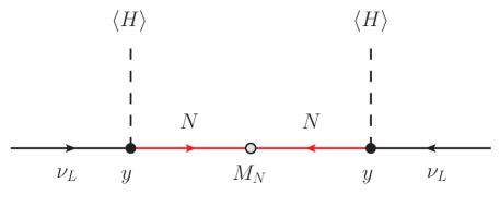
Figure 1: Neutrino mass generation in the type-I seesaw.

III.1.1 $3$ right-handed neutrinos

We can now adopt the common choice $r=r_{m}=3$, which implies $C_{1}=C_{2}=\mathbb{I}_{3}$. In this case, imposing $y_{1}=y_{2}$ is equivalent to $W^{T}WA=B$. Solving this matrix equation leads to $B=\left(A^{T}\right)^{-1}$ and allows one to define $R=W\,T=W\,A$, with $R$ a general $3\times 3$ orthogonal matrix. Replacing all these ingredients into Eqs. (6) and (9) one finds

$$y=\sqrt{2}\,y_{1}=\sqrt{2}\,y_{2}=i\,\Sigma^{-1/2}\,R\,D_{\sqrt{m}}\,U^{\dagger}\,,$$ (64)

which is nothing but the Casas-Ibarra parametrization for the type-I seesaw Yukawa matrices. We note that $R$ can be identified with the usual Casas-Ibarra matrix Casas:2001sr . We conclude that the Casas-Ibarra parametrization can be regarded as a particular case of the general master parametrization.

As a final comment, we note that in the type-I seesaw with $3$ generations of right-handed neutrinos, the condition $y_{1}=y_{2}$ implies $18\,(=9\cdot 2)$ real constraints, this is, $\texttt{\#}_{\rm extra}=18$. Therefore, direct application of the general counting formula in Eq. (53) leads to $\texttt{\#}_{\rm free}=6$. These are the free real parameters contained in the Casas-Ibarra $R$ matrix, which can be parametrized by means of $3$ complex angles, see Appendix B.

III.1.2 $2$ right-handed neutrinos

In the type-I seesaw with $2$ generations of right-handed neutrinos one also obtains the neutrino mass matrix in Eq. (62), but with $n_{1}=n_{2}=n=r=2$. Moreover, it is well known that in this case one induces only two non-vanishing neutrino mass eigenvalues, and hence $r_{m}=2$ and the model belongs either to the $(2,2)_{a}$ case or to the $(2,2)_{b}$ case. One can now follow a similar approach as for the $3$ generation model. In the $2$ generation version, imposing $y_{1}=y_{2}$ is equivalent to $W^{T}WA=B\leftrightarrow T^{T}\,W^{T}\,W\,T\,C_{1}=C_{1}\,C_{2}+KC_{1}$. Replacing the expressions for $C_{1}$ and $C_{2}$ in the $(2,2)_{b}$ case, one can easily find that this matrix equation leads to a contradiction. In case of neutrino NH this is found by comparing the elements $(1,2)$ and $(1,3)$, whereas in case of IH by comparing the elements $(1,1)$ and $(1,2)$. Therefore, we discard this scenario. Solving the matrix equation (decomposing it by elements) in the $(2,2)_{a}$ case, leads to $z_{1}=z_{2}=0$, $K=0$ and $R=W\,T$, with $R$ a general $2\times 2$ orthogonal matrix that can be parametrized by one complex angle. In summary, replacing all these ingredients into Eqs. (6) and (9) one finds

$$y=\sqrt{2}\,y_{1}=\sqrt{2}\,y_{2}=i\,\Sigma^{-1/2}\,R\,\left(\begin{array}[]{ccc}0&\sqrt{m_{2}}&0\\ 0&0&\sqrt{m_{3}}\end{array}\right)\,P\,U^{\dagger}\,,$$ (65)

where $P=\mathbb{I}_{3}$ in case of NH and $P=P_{13}$ and in case of IH, see Eqs. (11) and (12). In case of IH one should also rename $m_{3}\to m_{1}$. The result in Eq. (65) agrees perfectly with Ibarra:2003up .

III.2 The inverse seesaw

	spin	generations	$\mathrm{SU(3)}_{c}$	$\mathrm{SU(2)}_{L}$	$\mathrm{U(1)}_{Y}$
$N$	1/2	3	${\bf 1}$	${\bf 1}$	$0$
$S$	1/2	3	${\bf 1}$	${\bf 1}$	$0$

Table 4: New particles in the inverse seesaw.

We now consider the inverse seesaw Mohapatra:1986bd , an example model in which the matrix $M$ is actually the product of several matrices. In the inverse seesaw, the SM particle content is extended with the addition of $3$ generations of right-handed neutrinos $N$ and $3$ generations of singlet fermions $S$, both with lepton number $+1$, as summarized in Tab. 4.  The Lagrangian is assumed to contain the following terms involving these fields

$$-\mathcal{L}_{\rm ISS}=y\,H\,\overline{N}\,L+M_{R}\,\overline{N}\,S+\frac{1}{2}\mu\,\overline{S^{c}}S+\mathrm{h.c.}\,,$$ (66)

where we omit flavor indices to simplify the notation. $y$ is a general $3\times 3$ Yukawa matrix, $M_{R}$ is an arbitrary complex $3\times 3$ mass matrix while $\mu$ is a $3\times 3$ complex symmetric mass matrix. Again, the scalar potential and symmetry breaking pattern of the model is the same as in the SM. After symmetry breaking, the left-handed neutrinos $\nu_{L}$ mix with the $N$ and $S$ singlet fermions. In the basis $(\nu_{L}\,,\;N^{c}\,,\;S)$, the resulting $9\times 9$ neutral fermion mass matrix is given by

$$\mathcal{M}_{\rm ISS}=\left(\begin{array}[]{c c c}0&m_{D}^{T}&0\\ m_{D}&0&M_{R}\\ 0&M_{R}^{T}&\mu\end{array}\right)\,.$$ (67)

We note that in the absence of the $\mu$ term, the matrix in Eq. (67) would have a Dirac structure and lead to three massless states. In fact, $\mu$ violates lepton number by two units and can be taken naturally small, in the sense of ’t Hooft tHooft:1979rat , since the limit $\mu\to 0$ restores lepton number and increases the symmetry of the model. Under the assumption $\mu\ll m_{D}\ll M_{R}$, the mass matrix $\mathcal{M}_{\rm ISS}$ can be block-diagonalized to give an effective mass matrix for the $3$ light neutrinos GonzalezGarcia:1988rw

$$m_{\rm ISS}=m_{D}^{T}\,{M_{R}^{T}}^{-1}\,\mu\,M_{R}^{-1}\,m_{D}=\frac{v^{2}}{2}\,y^{T}\,{M_{R}^{T}}^{-1}\,\mu\,M_{R}^{-1}\,y\,.$$ (68)

Eq. (68) is shown diagrammatically in Fig. 2. Again, we can compare the inverse seesaw neutrino mass matrix in Eq. (68) to the general master formula in Eq. (1) and establish a dictionary: 

$$f=1$$

$$n_{1}=n_{2}=3$$

$$y_{1}=y_{2}=\frac{y}{\sqrt{2}}$$

$$M=\frac{v^{2}}{2}\,{M_{R}^{T}}^{-1}\,\mu\,M_{R}^{-1}$$ (69)

This identification clearly shows that one can make use of an adapted Casas-Ibarra parametrization for the inverse seesaw Deppisch:2004fa .

Figure 2: Neutrino mass generation in the inverse seesaw.

However, compared to the simpler type-I seesaw, discussed above, here $M$ can not be taken taken to be diagonal automatically and $V_{1}=V_{2}$ become physical. (Note that the two rotation matrices are still equal, since $M$ is a complex symmetric matrix in the inverse seesaw.) The reason for this is straightforward: $M$ contains the two matrices $M_{R}$ and $\mu$. If $y$ is taken arbitrary, we can still use field redefinitions for $N$ and $S$ to choose either $M_{R}$ or $\mu$ diagonal, but not both at the same time.

III.3 The scotogenic model

This example illustrates the use of the master parametrization in a model with loop induced neutrino masses. As we will show below, the radiative origin of neutrino masses does not alter the application of the master parametrization.

The scotogenic model Ma:2006km extends the SM particle content with three generations of the singlet fermions $N$ and the $SU(2)_{L}$ doublet scalar $\eta$. In addition, a $\mathbb{Z}_{2}$ symmetry is imposed, under which the new particles are odd while the SM ones are assumed to be even. The quantum numbers of the new particles in the scotogenic model are given in Table 5.

In addition to the canonical kinetic term, the Lagrangian contains the following terms involving the singlet fermions,

$$-\mathcal{L}_{\rm SC}=y\,\eta\,\overline{N}\,L+\frac{M_{N}}{2}\,\overline{N^{c}}\,N+\mathrm{h.c.}\,,$$ (70)

where we omit flavor indices for the sake of clarity. Here $M_{N}$ is a $3\times 3$ symmetric matrix with dimensions of mass which can be taken to be diagonal without loss of generality. The matrix of Yukawa couplings, $y$, is an arbitrary $3\times 3$ complex matrix. The scalar potential of the model is given by

$$\mathcal{V}_{\rm SC}= \>m_{H}^{2}H^{\dagger}H+m_{\eta}^{2}\eta^{\dagger}\eta+\frac{\lambda_{1}}{2}\left(H^{\dagger}H\right)^{2}+\frac{\lambda_{2}}{2}\left(\eta^{\dagger}\eta\right)^{2}+\lambda_{3}\left(H^{\dagger}H\right)\left(\eta^{\dagger}\eta\right)$$

$$+\lambda_{4}\left(H^{\dagger}\eta\right)\left(\eta^{\dagger}H\right)+\left[\frac{\lambda_{5}}{2}\left(H^{\dagger}\eta\right)^{2}+\frac{\lambda_{5}^{\ast}}{2}\left(\eta^{\dagger}H\right)^{2}\right]\,.$$ (71)

All parameters in the scalar potential are real, with the exception of the $\lambda_{5}$ quartic parameter, which can be complex. In the scotogenic model, the $\mathbb{Z}_{2}$ parity is assumed to be preserved after symmetry breaking. This is guaranteed by choosing a set of parameters that leads to a vacuum with

$$\langle H^{0}\rangle=\frac{v}{\sqrt{2}}\quad,\quad\langle\eta^{0}\rangle=0\,.$$ (72)

After electroweak symmetry breaking, the masses of the charged component $\eta^{+}$ and neutral component $\eta^{0}=(\eta_{R}+i\,\eta_{I})/\sqrt{2}$ are split to

$$m_{\eta^{+}}^{2} = m_{\eta}^{2}+\lambda_{3}\langle H^{0}\rangle^{2}\,,$$ (73)

$$m_{R}^{2} = m_{\eta}^{2}+\left(\lambda_{3}+\lambda_{4}+\lambda_{5}\right)\langle H^{0}\rangle^{2}\,,$$ (74)

$$m_{I}^{2} = m_{\eta}^{2}+\left(\lambda_{3}+\lambda_{4}-\lambda_{5}\right)\langle H^{0}\rangle^{2}\,.$$ (75)

We note that the mass difference between $\eta_{R}$ and $\eta_{I}$ (the CP-even and CP-odd components of the neutral $\eta^{0}$, respectively) is controlled by the $\lambda_{5}$ coupling since $m_{R}^{2}-m_{I}^{2}=2\lambda_{5}\langle H^{0}\rangle^{2}$. This will be relevant for the generation of non-vanishing neutrino masses in this model.

One of the most attractive features of the scotogenic model is the presence of a dark matter candidate. Indeed, the conservation of the $\mathbb{Z}_{2}$ symmetry implies that the lightest state charged under this parity is completely stable and, in principle, can serve as a good dark matter candidate. This role can be played by the lightest singlet fermion ($N_{1}$) or by the neutral component of the inert $\eta$ doublet ($\eta_{R}$ or $\eta_{I}$).

	spin	generations	$\mathrm{SU(3)}_{c}$	$\mathrm{SU(2)}_{L}$	$\mathrm{U(1)}_{Y}$	$\mathbb{Z}_{2}$
$\eta$	0	1	${\bf 1}$	${\bf 2}$	$1/2$	$-$
$N$	1/2	3	${\bf 1}$	${\bf 1}$	$0$	$-$

Table 5: New particles in the scotogenic model.

Figure 3: Neutrino mass generation in the scotogenic model.

We now move to the discussion of neutrino masses. First, we note that the singlet fermions do not couple to the SM Higgs doublet due to the $\mathbb{Z}_{2}$ discrete symmetry while $\langle\eta^{0}\rangle=0$ prevents the $\eta\,\overline{N}\,L$ Yukawa term from inducing a Dirac mass term for the neutrinos. Therefore, neutrino masses vanish at tree-level but get induced at the 1-loop level, as shown in Fig. 3. The resulting $3\times 3$ Majorana neutrino mass matrix is given by

$$\left(m_{\rm SC}\right)_{\alpha\beta} =\sum_{i=1}^{3}\frac{y_{i\alpha}y_{i\beta}}{2(4\pi)^{2}}M_{N_{i}}\left[\frac{m_{R}^{2}}{m_{R}^{2}-M_{N_{i}}^{2}}\log\left(\frac{m_{R}^{2}}{M_{N_{i}}^{2}}\right)-\frac{m_{I}^{2}}{m_{I}^{2}-M_{N_{i}}^{2}}\log\left(\frac{m_{I}^{2}}{M_{N_{i}}^{2}}\right)\right]\,,$$ (76)

$$\equiv\frac{1}{32\pi^{2}}\left(y^{T}\,{\widehat{M}}\,y\right)_{\alpha\beta}\,,$$ (77)

with the diagonal matrix ${\widehat{M}}$ with entries

$${\widehat{M}}_{ii}=M_{N_{i}}\left[\frac{m_{R}^{2}}{m_{R}^{2}-M_{N_{i}}^{2}}\log\left(\frac{m_{R}^{2}}{M_{N_{i}}^{2}}\right)-\frac{m_{I}^{2}}{m_{I}^{2}-M_{N_{i}}^{2}}\log\left(\frac{m_{I}^{2}}{M_{N_{i}}^{2}}\right)\right]\,,$$ (78)

A simplified expression can be obtained when $m_{R}^{2}\approx m_{I}^{2}\equiv m_{0}^{2}$ (or, equivalently, $\lambda_{5}\ll 1$). In this case, Eq. (76) reduces to 

$$\left(m_{\rm SC}\right)_{\alpha\beta} \simeq\sum_{i=1}^{3}\frac{\lambda_{5}y_{i\alpha}y_{i\beta}\langle H^{0}\rangle^{2}}{(4\pi)^{2}M_{N_{i}}}\left[\frac{M_{N_{i}}^{2}}{m_{0}^{2}-M_{N_{i}}^{2}}+\frac{M_{N_{i}}^{4}}{\left(m_{0}^{2}-M_{N_{i}}^{2}\right)^{2}}\log\left(\frac{M_{N_{i}}^{2}}{m_{0}^{2}}\right)\right]$$

$$\equiv\frac{\lambda_{5}}{16\pi^{2}}\left(y^{T}\Lambda\,y\right)_{\alpha\beta}\,,$$ (79)

where we have defined $\Lambda=\text{diag}\left(\Lambda_{1},\Lambda_{2},\Lambda_{3}\right)$, with

$$\Lambda_{i}=\frac{\langle H^{0}\rangle^{2}}{M_{N_{i}}}\left[\frac{M_{N_{i}}^{2}}{m_{0}^{2}-M_{N_{i}}^{2}}+\frac{M_{N_{i}}^{4}}{\left(m_{0}^{2}-M_{N_{i}}^{2}\right)^{2}}\log\left(\frac{M_{N_{i}}^{2}}{m_{0}^{2}}\right)\right]\,.$$ (80)

Eq. (77) and the last equality of Eq. (III.3) clearly shows that the Yukawa matrix $y$ can be written using an adapted Casas-Ibarra parametrization Toma:2013zsa . In fact, direct comparison to the master formula in Eq. (1) allows one to identify

$$f=\frac{\lambda_{5}}{16\pi^{2}}$$

$$n_{1}=n_{2}=3$$

$$y_{1}=y_{2}=\frac{y}{\sqrt{2}}$$

$$M=\Lambda$$ (81)

in the scotogenic model.

III.4 The linear seesaw

The full power of the master parametrization is better illustrated with an application to the linear seesaw Akhmedov:1995ip ; Akhmedov:1995vm , which provides a well-known example of a neutrino mass formula with $y_{1}\neq y_{2}$.

	spin	generations	$\mathrm{SU(3)}_{c}$	$\mathrm{SU(2)}_{L}$	$\mathrm{U(1)}_{Y}$
$N$	1/2	3	${\bf 1}$	${\bf 1}$	$0$
$S$	1/2	3	${\bf 1}$	${\bf 1}$	$0$

Table 6: New particles in the linear seesaw.

Originally introduced in the context of left-right symmetric models Akhmedov:1995ip ; Akhmedov:1995vm , this mechanism has also been shown to arise naturally in $\mathrm{SO(10)}$ unified theories Barr:2003nn ; Malinsky:2005bi . The particle content of the model is the same as in the inverse seesaw, as shown in Tab. 6. The Lagrangian is assumed to contain the following terms

$$-\mathcal{L}_{\rm LSS}=y\,H\,\overline{N}\,L+M_{R}\,\overline{N}\,S+y_{L}\,H\,\overline{L^{c}}\,S+\mathrm{h.c.}\,,$$ (82)

where again we omit flavor indices to simplify the notation. As in the inverse seesaw, $y$ is a general $3\times 3$ Yukawa matrix and $M_{R}$ is a $3\times 3$ complex mass matrix. In addition, $y_{L}$ is a general $3\times 3$ Yukawa matrix, with $y_{L}\neq y$ in general. Therefore, the linear seesaw model features $y_{1}\neq y_{2}$. The scalar potential and symmetry breaking pattern of the model is the same as in the SM. In the basis $(\nu_{L}\,,\;N^{c}\,,\;S)$, the resulting $9\times 9$ neutral fermion mass matrix obtained after electroweak symmetry breaking takes the form

$$\mathcal{M}_{\rm LSS}=\left(\begin{array}[]{c c c}0&m_{D}^{T}&M_{L}\\ m_{D}&0&M_{R}\\ M_{L}^{T}&M_{R}^{T}&0\end{array}\right)\,,$$ (83)

where $M_{L}=\frac{1}{\sqrt{2}}\,y_{L}v$. We note that in the presence of $M_{L}$, lepton number is broken in two units. Assuming $m_{D},M_{L}\ll M_{R}$, the mass matrix for the $3$ light neutrinos is given by

$$m_{\rm LSS}=M_{L}\,M_{R}^{-1}\,m_{D}+m_{D}^{T}\,{M_{R}^{T}}^{-1}\,M_{L}^{T}=\frac{v^{2}}{2}\,\left(y_{L}\,M_{R}^{-1}\,y+y^{T}\,{M_{R}^{T}}^{-1}\,y_{L}^{T}\right)\,.$$ (84)

Eq. (84) is shown diagrammatically in Fig. 4 (without the transposed 2nd term). We see that the resulting expression for the light neutrino mass matrix is linear in $y$ (or, equivalently, in $m_{D}$), hence the origin of the name linear seesaw. As usual, we now compare the linear seesaw neutrino mass matrix in Eq. (84) to the general master formula in Eq. (1). By doing so one finds the following dictionary:

$$f=1$$

$$n_{1}=n_{2}=3$$

$$y_{1}=y_{L}^{T}$$

$$y_{2}=y$$

$$M=\frac{v^{2}}{2}\,M_{R}^{-1}$$ (85)

We emphasize again that one cannot make use of the standard Casas-Ibarra parametrization in the linear seesaw model due to $y\neq y_{L}^{T}$ (a particular example of the general case $y_{1}\neq y_{2}$). In this case one must necessarily make use of the full master parametrization.

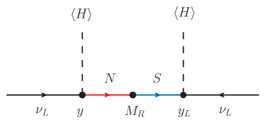
Figure 4: Neutrino mass generation in the linear seesaw.

IV Models with extra symmetries and restrictions

We now discuss Majorana neutrino mass models which follow the structure of Eq. (1), but the master parametrization may become either not direct, impractical or useless. These “exceptional” cases are simply those for which $y_{1}$ and $y_{2}$ are not completely free parameters. Based on the type of restrictions, the $y_{1}$ and $y_{2}$ Yukawa matrices must follow, one can identify four categories:

1. Identity models: $y_{1}=y_{2}=\mathbb{I}$. This is the case of the seesaw type-II and similar models.

2. Symmetric models: $y_{1}=y_{1}^{T}$ and/or $y_{2}=y_{2}^{T}$. This is the case in many models with an underlying left-right symmetry.

3. Antisymmetric models: $y_{1}=-y_{1}^{T}$ and/or $y_{2}=-y_{2}^{T}$. This scenario takes place in models including the charged scalar $s$, which transforms as $({\bf 1},{\bf 1},1)$ under the SM gauge symmetry, due to the presence of the antisymmetric $\rm SU(2)_{L}$ contraction in the $s\,\overline{L^{c}}\,L$ Yukawa term. Two well known examples of such scenario are the Zee ($y_{1}=-y_{1}^{T}$) and Zee-Babu ($\sqrt{2}\,y_{1}=\sqrt{2}\,y_{2}=y$, with $y=-y^{T}$) models.

4. Flavored models: specific textures in $y_{1}$ and $y_{2}$. This would be the case of models with flavor symmetries. Models with conditions on the $y_{1}$ and $y_{2}$ Yukawa matrices not included in the previous cases can be generically included here.

As discussed next, case (i) is trivial, whereas case (ii) needs only a slight modification of our procedure. Only cases (iii) and (iv) are not so easily solved and require an in-depth discussion.

Identity models, those with $y_{1}=y_{2}=\mathbb{I}$, are trivially addressed. For instance, let us consider the type-II seesaw Mohapatra:1980yp ; Schechter:1980gr . This model extends the SM particle content with the $\rm SU(2)_{L}$ triplet scalar $\Delta$ with hypercharge $Y_{\Delta}=1$. The inclusion of this field allows us to write the Yukawa term $Y_{\Delta}\,\overline{L^{c}}\,\Delta\,L$ which, after the neutral component of $\Delta$ acquires a VEV, $v_{\Delta}$, induces Majorana masses for the neutrinos, with their mass matrix given by $m=Y_{\Delta}\,v_{\Delta}$. It is clear that this model can also be described by means of the master formula, with the dictionary simply given by

$$f=1$$

$$n_{1}=n_{2}=3$$

$$y_{1}=y_{2}=\mathbb{I}_{3}$$

$$M=Y_{\Delta}\,v_{\Delta}$$ (86)

Even though the master formula also includes models in this category, they do not require a parametrization for the Yukawa matrices. Note that the neutrino mixing matrix is simply given by the diagonalization matrix of $Y_{\Delta}$.

In what concerns symmetric models, a simple yet elegant solution when $y_{1}=y_{2}$ was given in Anamiati:2016uxp . We proceed to reproduce it here. Let us consider a fully symmetric type-I seesaw neutrino mass matrix with $\sqrt{2}\,y_{1}=\sqrt{2}\,y_{2}=y=y^{T}$. The master formula reduces to $m=y^{T}My\equiv yMy$ and the master parametrization to a Casas-Ibarra parametrization, see Eq. (64). $M$ must be a symmetric matrix in this case, and then it can be brought to a diagonal form with just a single matrix $V$,

$$M=V^{T}\,\widehat{\Sigma}\,V\,,$$ (87)

and the Casas-Ibarra parametrization reads

$$y=i\,V^{\dagger}\,\Sigma^{-1/2}\,R\,D_{\sqrt{m}}\,U^{\dagger}\,,$$ (88)

with $R$ a complex orthogonal $3\times 3$ matrix. This equation can be trivially rewritten as

$$Y=V\,y=i\,\Sigma^{-1/2}\,R\,D_{\sqrt{m}}\,U^{\dagger}\,.$$ (89)

This shows that the matrix $Y$ can be obtained by applying a standard Casas-Ibarra parametrization. The key now is to be able to decompose it as the product of the unitary matrix $V$ and the symmetric matrix $y$. In order to do that we first apply a singular-value decomposition,

$$Y=W_{1}^{T}\,\widehat{Y}\,W_{2}\,,$$ (90)

where $W_{1}$ and $W_{2}$ are two unitary matrices and $\widehat{Y}$ is a diagonal matrix containing the (real and non-negative) singular values of $Y$. We can now insert $W_{2}^{\ast}W_{2}^{T}=\mathbb{I}_{3}$ to obtain

$$Y=W_{1}^{T}\,\widehat{Y}\,W_{2}=\left(W_{1}^{T}\,W_{2}^{\ast}\right)\,\left(W_{2}^{T}\,\widehat{Y}\,W_{2}\right)\equiv\widetilde{V}\,\widetilde{y}\,,$$ (91)

where we have identified the unitary matrix $\widetilde{V}=W_{1}^{T}\,W_{2}^{\ast}$ and the symmetric matrix $\widetilde{y}=W_{2}^{T}\,\widehat{Y}\,W_{2}$. As explained in Anamiati:2016uxp , $\widetilde{V}$ and $\widetilde{y}$ are not unique, simply because the singular-value decomposition is not unique. One can always define

$$W_{1}^{\prime} =D_{\phi}\,W_{1}\,,$$ (92)

$$W_{2}^{\prime} =D_{\phi}^{-1}\,W_{2}\,,$$ (93)

with

$$D_{\phi}=\text{diag}\left(e^{i\phi_{1}},e^{i\phi_{2}},e^{i\phi_{3}}\right)$$ (94)

a diagonal phase matrix, such that $Y=W_{1}^{\prime\,T}\,\widehat{Y}\,W_{2}^{\prime}$ as well.  These three phases must be taken into account in the factorization of $Y$ as the product of a unitary matrix and a symmetric matrix. We then make the identification

$$V =W_{1}^{T}\,D_{\phi}^{-1}\,W_{2}^{\ast}\,,$$ (95)

$$y =W_{2}^{T}\,D_{\phi}\,\widehat{Y}\,W_{2}\,,$$ (96)

which preserves $Y=V\,y$ and the symmetric nature of $y$. In summary, when both Yukawa matrices are equal and symmetric, one can use the standard Casas-Ibarra parametrization for $Y$ and finally find $y$ by means of the decomposition in Eq. (96).

Finally, we come to case (iii), models with antisymmetric Yukawa matrices. We first consider the scenario with one antisymmetric Yukawa coupling, $y_{1}=-y_{1}^{T}$, with general $y_{2}$. The most popular model of this class is the Zee model Zee:1980ai , discussed in Sec. IV.1. As in the general case, both Yukawa matrices, $y_{1}$ and $y_{2}$, can be written using the master parametrization in Eqs. (6) and (9). However, the antisymmetry of $y_{1}$ implies some non-trivial conditions on the matrices $W$ and $T$, as well as on $m$ and $M$. Therefore, the input matrices $m$ and $M$ can no longer be arbitrary, but are indeed forced to follow some relations if the master formula in Eq. (1) is to be satisfied. More details about this scenario with one antisymmetric Yukawa coupling can be found in Appendix C. Now we turn to the special case of equal and antisymmetric Yukawa matrices, $\sqrt{2}\,y_{1}=\sqrt{2}\,y_{2}=y=-y^{T}$. The Zee-Babu model Cheng:1980qt ; Zee:1985id ; Babu:1988ki , presented in detail in Sec. IV.2, is the most popular model of this class. In this scenario one necessarily has $n_{1}=n_{2}=3$, $V_{1}=V_{2}\equiv V$ and $r=r_{m}=2$. The master formula reduces to $m=y^{T}My=-yMy$ and the master parametrization to a modified Casas-Ibarra parametrization. In case of $n=3$ one finds

$$y=\sqrt{2}\,y_{1}=\sqrt{2}\,y_{2}=i\,V^{\dagger}\,\Sigma^{-1/2}\,R\,C_{1}\,\bar{D}_{\sqrt{m}}\,U^{\dagger}\,,$$ (97)

with $C_{1}$ given in Eq. (41), in this case fixing $z_{1}=z_{2}=0$, and $R$ a $3\times 2$ Casas-Ibarra matrix such that $R^{T}R=\mathbb{I}_{2}$. However, the parametrization for the $y$ matrix in Eq. (97) is not sufficient to guarantee the antisymmetry of the $y$ Yukawa matrix. Many additional restrictions must be taken into account. In fact, the equality $\sqrt{2}\,y_{1}=\sqrt{2}\,y_{2}=y=-y^{T}$ implies 12 (real) conditions. Since the number of real free parameters in this scenario is 6, the system is overconstrained. This has two implications. First, in contrast to the general case, $R$ must take a very specific form. And second, the parameters in $m$ and $M$ are not free anymore, but they are indeed forced to follow 6 real conditions: one vanishing neutrino mass eigenvalue, one vanishing Majorana phase and two (complex) non-trivial conditions. For the proof and more details about this special case we refer to Appendix D.

Let us also comment on alternative approaches in case of antisymmetric Yukawa couplings. First, in models in which $M$ is a product of more than one matrix, it may be more practical to solve for (one of) the inner Yukawa couplings, instead of $y_{1}$ or $y_{2}$. And second, we are discussing a master parametrization which we later particularize to specific models. This approach is completely general and can be used for any Majorana neutrino mass model. However, in some particular cases there might be a simpler and more direct approach. For instance, a parametrization for the antisymmetric scenario with $\sqrt{2}\,y_{1}=\sqrt{2}\,y_{2}=y=-y^{T}$ was presented in Babu:2002uu . The antisymmetry of the $y$ matrix implies that

$$v_{0}=\begin{pmatrix}y_{23}\\ -y_{13}\\ y_{12}\end{pmatrix}$$ (98)

is an eigenvector of $y$ with null eigenvalue. Since $m=-yMy$, $v_{0}$ is also eigenvector of $m$ and we can write

$$m\,v_{0}=0\Leftrightarrow U^{\ast}\,D_{m}\,U^{\dagger}\,v_{0}=0\Leftrightarrow D_{m}\,U^{\dagger}\,v_{0}=0\,.$$ (99)

This equation can be solved analytically to determine two of the components of $v_{0}$ in terms of the third and the neutrino masses and mixing angles contained in $D_{m}$ and $U$. Furthermore, as explained above, the matrix $M$ is not free in this special case. The conditions on its entries can be derived by replacing the form for $y$ obtained with Eq. (99) into $m=U^{\ast}\,D_{m}\,U^{\dagger}=-yMy$. Out of the six equations, only three are independent. Therefore, one can obtain three $M$ entries in terms of the remaining parameters. For instance, one can choose to solve the equations for $M_{22}$, $M_{23}$ and $M_{33}$. This solution has been found to be very convenient for phenomenological studies Herrero-Garcia:2014hfa . Nevertheless, we emphasize again that our focus is on the generality of our approach, while this type of solutions can only be applied to very specific scenarios.

Finally, the number of possible restrictions in flavored models is enormous and a systematic exploration is not feasible. For this reason, we will not discuss them here, although we note that the master parametrization might provide a powerful analytical tool for the treatment of these special cases. We also point out that in some models the charged lepton mass matrix is not diagonal in the flavor basis. Instead, the mass and flavor bases are related by

$$\widehat{m}_{e}=U_{e}^{\dagger}\,m_{e}\,V_{e}\,,$$ (100)

where $m_{e}$ and $\widehat{m}_{e}$ are the charged lepton mass matrix in the flavor and mass bases, respectively, and $U_{e}$ and $V_{e}$ are two $3\times 3$ unitary matrices. This would introduce an additional unitary matrix in the master parametrization, replacing $U^{\dagger}$ in Eqs. (6) and (9) by $U^{\dagger}\,U_{e}^{\dagger}$.

We now present two models of type (iii), the Zee and Zee-Babu models. They constitute well-known examples of models with antisymmetric Yukawa couplings.

IV.1 The Zee model

	spin	generations	$\mathrm{SU(3)}_{c}$	$\mathrm{SU(2)}_{L}$	$\mathrm{U(1)}_{Y}$
$\phi$	0	1	${\bf 1}$	${\bf 2}$	$1/2$
$s$	0	1	${\bf 1}$	${\bf 1}$	$1$

Table 7: New particles in the Zee model.

The Zee model Zee:1980ai constitutes a very simple scenario beyond the SM leading to radiative neutrino masses. The particle content of the SM is extended to include a second Higgs doublet, $\phi$, and the $\rm SU(2)_{L}$ singlet scalars $s$, with hypercharge $+1$. Therefore, the Zee model can be regarded as an extension of the general Two Higgs Doublet Model (THDM) by a charged scalar. As we will see below, the presence of this singly-charged scalar has a strong impact on the structure of the Yukawa matrix relevant for the generation of neutrino masses. The new states in the Zee model are summarized in Tab. 7. With them, the Yukawa Lagrangian of the model includes

$$-\mathcal{L}^{Y}_{\rm Z}=\overline{L}\left(y_{e}\,H+\Gamma_{e}\,\phi\right)\,e_{R}+y_{s}\,s\,\overline{L^{c}}\,L+\mathrm{h.c.}\,,$$ (101)

where flavor indices have been omitted. The $3\times 3$ Yukawa matrix $y_{s}$ is antisymmetric in flavor space while $y_{e}$ and $\Gamma_{e}$ are two general $3\times 3$ complex matrices. In the general THDM, both Higgs doublets could acquire non-zero VEVs. However, with no quantum number distinguishing $H$ and $\phi$, one can choose to go to the so-called Higgs basis, in which only one of the two fields acquires a VEV. We choose that the electroweak VEV $v$ is obtained as $v^{2}=v_{H}^{2}$. In this basis, the expressions for the mass matrices become especially simple. In case of the charged leptons, this reads

$$\mathcal{M}_{e}=\frac{v}{\sqrt{2}}\,y_{e}\,.$$ (102)

In the following, and without loss of generality, we will work in the basis in which $\mathcal{M}_{e}$ is diagonal. The scalar potential of the Zee model includes the trilinear term

$$\mathcal{V}_{\rm Z}\supset\mu_{\rm Z}\,H\,\phi\,s^{\ast}+\mathrm{h.c.}\,,$$ (103)

where $\mu_{\rm Z}$ is a parameter with dimensions of mass. After electroweak symmetry breaking, this trilinear coupling leads to mixing between the usual charged Higgs of the THDM and $s\equiv s^{+}$. The mixing angle, denoted as $\varphi$, is given by

$$s_{2\varphi}=\sin 2\varphi=\frac{\sqrt{2}\,v\,\mu_{\rm Z}}{m_{h_{2}^{+}}^{2}-m_{h_{1}^{+}}^{2}}\,,$$ (104)

where $m_{h_{1}^{+}}^{2}$ and $m_{h_{2}^{+}}^{2}$ are the squared masses of the two physical charged scalars in the spectrum, $h_{1}^{+}$ and $h_{2}^{+}$, respectively. The relevance of the trilinear $\mu_{\rm Z}$ goes beyond this mixing in the charged scalar sector. It is straightforward to show that a conserved lepton number cannot be defined in the presence of the Lagrangian terms in Eqs. (101) and (103). In fact, lepton number is explicitly violated in two units, leading to the generation of Majorana neutrino masses at the 1-loop level, as shown in Fig. 5. The neutrino mass matrix is calculable and given by

$$m_{\rm Z}=-\frac{s_{2\varphi}}{16\,\pi^{2}}\,\left(y_{s}\,\mathcal{M}_{e}\,\Gamma_{e}+\Gamma_{e}^{T}\,\mathcal{M}_{e}\,y_{s}^{T}\right)\,\log\left(\frac{m_{h_{2}^{+}}^{2}}{m_{h_{1}^{+}}^{2}}\right)\,.$$ (105)

Direct comparison with the master formula in Eq. (1) indicates that in the Zee model one has $y_{1}\neq y_{2}$. In fact, the Zee model constitutes a well-known example of a model in which one of the Yukawa matrices is antisymmetric while the other is a general complex matrix.

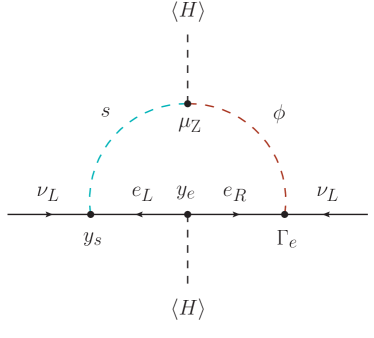
Figure 5: Neutrino mass generation in the Zee model.

IV.2 The Zee-Babu model

	spin	generations	$\mathrm{SU(3)}_{c}$	$\mathrm{SU(2)}_{L}$	$\mathrm{U(1)}_{Y}$
$s$	0	1	${\bf 1}$	${\bf 1}$	$1$
$k$	0	1	${\bf 1}$	${\bf 1}$	$2$

Table 8: New particles in the Zee-Babu model.

The Zee-Babu model Cheng:1980qt ; Zee:1985id ; Babu:1988ki is a simple extension of the scalar content of the SM. In addition to the usual Higgs doublet, two $\rm SU(2)_{L}$ singlet scalars are introduced: the singly-charged $s\equiv s^{+}$ and the doubly-charged $k\equiv k^{++}$. This is explicitly summarized in Tab. 8. With these fields, the Lagrangian includes two new Yukawa terms

$$-\mathcal{L}^{Y}_{\rm ZB}=y_{s}\,s\,\overline{L^{c}}\,L+g\,k\,\overline{e_{R}^{c}}\,e_{R}+\mathrm{h.c.}\,,$$ (106)

where flavor indices have been omitted. Here $y_{s}$ is an antisymmetric $3\times 3$ Yukawa matrix while $g$ is a symmetric $3\times 3$ matrix. In addition, the scalar potential of the model includes the trilinear term

$$\mathcal{V}_{\rm ZB}\supset\mu_{\rm ZB}\,s\,s\,k^{\ast}+\mathrm{h.c.}\,,$$ (107)

where $\mu_{\rm ZB}$ is a parameter with dimensions of mass. The simultaneous presence of the Lagrangian terms in Eqs. (106) and (107) implies the breaking of lepton number in two units. This leads to the generation of Majorana neutrino masses at the 2-loop level, as shown in Fig. 6. In this graph $y_{e}$ is the SM lepton Yukawa term, defined as $y_{e}\,H\,\overline{L}\,e_{R}$. The resulting expression for the neutrino mass matrix takes the form

$$m_{\rm ZB}=\frac{v^{2}\,\mu_{\rm ZB}}{(16\pi^{2})^{2}\,m_{s}^{2}}\,y_{s}\,y_{e}\,g\,y_{e}^{T}\,y_{s}^{T}\,F_{\rm ZB}\left(\frac{m_{k}^{2}}{m_{s}^{2}}\right)\,,$$ (108)

where $m_{s}$ and $m_{k}$ are the $s$ and $k$ squared masses, respectively, and $F_{\rm ZB}$ is a dimensionless loop function. Therefore, we see that in the Zee-Babu model one has $\sqrt{2}\,y_{1}=\sqrt{2}\,y_{2}=y_{s}$, with $y_{s}=-y_{s}^{T}$. This indeed implies a prediction: since $\text{Det}(y_{s})=0$, one of the neutrinos remains massless.

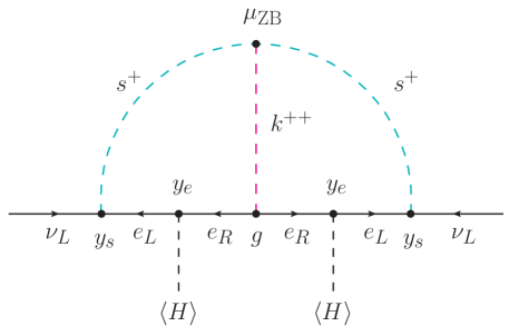
Figure 6: Neutrino mass generation in the Zee-Babu model.

V Summary

We have presented a general parametrization for the Yukawa couplings in Majorana neutrino mass models. We call this the master parametrization. A proof for the master parametrization has also been presented, see Appendix A. In order to help the reader in practical applications, we have also provided a Mathematica notebook that implements the master parametrization in masterweb . The aim of this master parametrization is to generalize the well-known Casas-Ibarra parametrization, which in its strict original form is valid only for the type-I seesaw. Although different adaptations of the Casas-Ibarra parametrization have been discussed in the context of concrete models in the literature, the aim of our master parametrization is to be as completely general as possible.

We stress that our master parametrization is valid for any Majorana neutrino mass model. We have shown its application to various well-known example models. We have also discussed some particular cases, where the Yukawa couplings are no longer completely free parameters but, typically for symmetry reasons, have to obey some restrictions. In such cases, the application of the master parametrization may become either trivial or impractically complicated, depending on the complexity of the extra conditions, as we discussed with some examples.

Let us briefly mention that from the list of examples that we have discussed in Section III, one should not derive the incorrect conclusion that only very few neutrino mass models require the full power of the master parametrization. This bias in our example list is mainly due to the fact that in our discussion we have focused on the best-known neutrino mass models that exist in the literature.

In fact, once one goes beyond the minimal $d=5$ tree-level realizations of the Weinberg operator, the majority of models have $y_{1}\neq y_{2}$ and the Casas-Ibarra parametrization can not cover these models, as we have stressed several times. At tree-level, at $d=7$ we find the BNT model Babu:2009aq at $d=9$ one of the two genuine models (model-II) in Anamiati:2018cuq is also of this type. Actually, for radiative neutrino mass models the majority of models are of this type. This can be easily understood as follows. Consider, for example, the neutrino mass model shown in Fig. 7. The diagram is the same as in the scotogenic model. Here, the vector-like fermion $\psi$ transforming as $({\bf 1},{\bf 3},1)$ (with its vector partner ${\bar{\psi}}$) replace the singlet fermions of the original model. In addition to $\eta$, a second doublet $\rho$ with quantum numbers $({\bf 1},{\bf 2},3/2)$ is introduced. This model obviously has two independent Yukawa couplings and thus, the full master parametrization is needed to describe its parameter space. Another example of a modified Scotogenic model with $y_{1}\neq y_{2}$ can be found in Ma:2013yga ; Hagedorn:2018spx . Unsurprisingly, at loop level there are actually more variations with this type of “asymmetric” diagrams, i.e. $y_{1}\neq y_{2}$, than variations with “symmetric” diagrams (where the field coupling to the two neutrinos is necessarily the same) as can be seen, for example, in the tables of Bonnet:2012kz ; Sierra:2014rxa or the list of diagrams at d=7 1-loop in Cepedello:2017eqf .

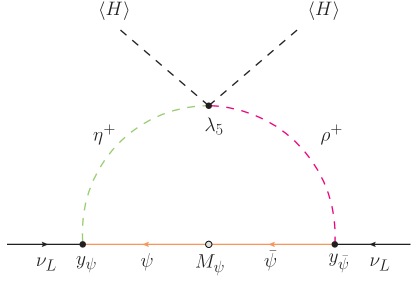
Figure 7: Neutrino mass generation in a modified scotogenic model, for defintions see text. This simple variation necessarily has two independent Yukawa couplings.

We close by mentioning again that we have concentrated our discussion on the particular case of three, light active neutrinos. It is possible to extend our approach to four or more neutrinos, if ever this becomes necessary. Technically, the form of our master parametrization would remain the same, but the dimensions of the defining matrices will change, and the explicit forms of the matrices $C_{1}$ and $C_{2}$, defined in Section II, would need to be calculated.

Appendix A Proof

In the following, we provide a constructive proof of the master parametrization. We begin by replacing the Takagi decomposition of $m$ in Eq. (2) and the singular-value decomposition of $M$ in Eq. (13) into the master formula in Eq. (1). Moreover, we take $f=1$ to simplify the expressions in the proof, and take this global factor into account by rescaling the final expressions for the $y_{1}$ and $y_{2}$ Yukawa matrices. This leads to

$$(U^{\dagger})^{T}\,D_{m}\,U^{\dagger}=y_{1}^{T}\,V_{1}^{T}\,\widehat{\Sigma}\,V_{2}\,y_{2}+y_{2}^{T}\,V_{2}^{T}\,\widehat{\Sigma}^{T}\,V_{1}\,y_{1}\,.$$ (109)

Multiplying the previous expression on the left by $(\bar{D}_{\sqrt{m}})^{-1}\,U^{T}$ and on the right by $U\,(\bar{D}_{\sqrt{m}})^{-1}$, with $\bar{D}_{\sqrt{m}}$ introduced in Eq. (10), one obtains

$$(\bar{D}_{\sqrt{m}})^{-1}\,D_{\sqrt{m}}\,D_{\sqrt{m}}\,(\bar{D}_{\sqrt{m}})^{-1}=$$

$$(\bar{D}_{\sqrt{m}})^{-1}\,U^{T}y_{1}^{T}\,V_{1}^{T}\,\widehat{\Sigma}\,V_{2}\,y_{2}\,U\,(\bar{D}_{\sqrt{m}})^{-1}+(\bar{D}_{\sqrt{m}})^{-1}\,U^{T}y_{2}^{T}\,V_{2}^{T}\,\widehat{\Sigma}^{T}\,V_{1}\,y_{1}\,U\,(\bar{D}_{\sqrt{m}})^{-1}\,.$$ (110)

This expression clearly suggests to introduce

$$\bar{y}_{1} =V_{1}\,y_{1}\,U\,(\bar{D}_{\sqrt{m}})^{-1}\,,$$ (111)

$$\bar{y}_{2} =V_{2}\,y_{2}\,U\,(\bar{D}_{\sqrt{m}})^{-1}\,.$$ (112)

We note that $y_{1}$ and $y_{2}$ can be univocally determined from $\bar{y}_{1}$ and $\bar{y}_{2}$, since all the other matrices participating in Eqs. (111) and (112) are invertible. With these definitions, Eq. (110) is equivalent to

$$\bar{y}_{1}^{T}\,\widehat{\Sigma}\,\bar{y}_{2}+\bar{y}_{2}^{T}\,\widehat{\Sigma}^{T}\,\bar{y}_{1}=\left\{\begin{array}[]{cr}\mathbb{I}_{3}&\text{if}\ r_{m}=3\,,\\ &\\ P\,\begin{pmatrix}0&0&0\\ 0&1&0\\ 0&0&1\end{pmatrix}\,P&\text{if}\ r_{m}=2\,.\end{array}\right.$$ (113)

In the next step, we write the matrices $\bar{y}_{1}$, $\bar{y}_{2}$ and $\widehat{\Sigma}$ in blocks. As we will see below, this will allow us to identify some arbitrary blocks and focus the discussion on the non-trivial ones. Using the general expression for $\widehat{\Sigma}$ given in Eq. (14), the combination $\bar{y}_{1}^{T}\,\widehat{\Sigma}\,\bar{y}_{2}+\bar{y}_{2}^{T}\,\widehat{\Sigma}^{T}\,\bar{y}_{1}$ in Eq. (113) can be written as

$$\bar{y}_{1}^{T}\,\widehat{\Sigma}\,\bar{y}_{2}+\bar{y}_{2}^{T}\,\widehat{\Sigma}^{T}\,\bar{y}_{1}=$$

$$\left((\bar{y}_{1})_{n}^{T}\;\;(\bar{y}_{1})_{n_{2}-n}^{T}\;\;(\bar{y}_{1})_{n_{1}-n_{2}}^{T}\right)\left(\begin{array}[]{c}\begin{array}[]{cc}\Sigma&0\\ 0&0_{n_{2}-n}\end{array}\\ \hline\cr 0_{n_{1}-n_{2}}\end{array}\right)\left(\begin{array}[]{c}(\bar{y}_{2})_{n}\\ (\bar{y}_{2})_{n_{2}-n}\end{array}\right)+\left((\bar{y}_{2})_{n}^{T}\;\;(\bar{y}_{2})_{n_{2}-n}^{T}\right)\left(\begin{array}[]{c|c}\begin{array}[]{cc}\Sigma&0\\ 0&0^{T}_{n_{2}-n}\end{array}&0^{T}_{n_{1}-n_{2}}\end{array}\right)\left(\begin{array}[]{c}(\bar{y}_{1})_{n}\\ (\bar{y}_{1})_{n_{2}-n}\\ (\bar{y}_{1})_{n_{1}-n_{2}}\end{array}\right)$$ (126)

$$=(\bar{y}_{1})_{n}^{T}\,\Sigma\,(\bar{y}_{2})_{n}+(\bar{y}_{2})_{n}^{T}\,\Sigma\,(\bar{y}_{1})_{n}\,.$$ (127)

We clearly see that there are some blocks which can have arbitrary values since they multiply null matrices and drop in the final expression. These are

$$X_{1} =\sqrt{2}\,(\bar{y}_{1})_{n_{2}-n}\in\mathbb{C}^{(n_{2}-n)\times 3}\,,$$

$$X_{2} =\sqrt{2}\,(\bar{y}_{1})_{n_{1}-n_{2}}\in\mathbb{C}^{(n_{1}-n_{2})\times 3}\,,$$

$$X_{3} =\sqrt{2}\,(\bar{y}_{2})_{n_{2}-n}\in\mathbb{C}^{(n_{2}-n)\times 3}\,,$$ (128)

where the $\sqrt{2}$ factors have been introduced for convenience. $X_{1}$, $X_{2}$ and $X_{3}$ have $6(n_{2}-n)$, $6(n_{1}-n_{2})$ and $6(n_{2}-n)$ free real parameters, respectively. We define now

$$\bar{\bar{y}}_{1} =\sqrt{2}\,\Sigma^{1/2}\,(\bar{y}_{1})_{n}\,,$$ (129)

$$\bar{\bar{y}}_{2} =\sqrt{2}\,\Sigma^{1/2}\,(\bar{y}_{2})_{n}\,.$$ (130)

Again, $\bar{y}_{1}$ and $\bar{y}_{2}$, and hence the original Yukawa matrices $y_{1}$ and $y_{2}$, can be univocally obtained from $\bar{\bar{y}}_{1}$ and $\bar{\bar{y}}_{2}$ since the matrix $\Sigma^{1/2}$ is invertible. With these redefinitions, Eq. (113) is equivalent to

$$\bar{\bar{y}}_{1}^{T}\,\bar{\bar{y}}_{2}+\bar{\bar{y}}_{2}^{T}\,\bar{\bar{y}}_{1}=\left\{\begin{array}[]{cr}2\,\mathbb{I}_{3}&\text{if}\ r_{m}=3\,,\\ &\\ 2\,P\,\begin{pmatrix}0&0&0\\ 0&1&0\\ 0&0&1\end{pmatrix}\,P&\text{if}\ r_{m}=2\,.\end{array}\right.$$ (131)

At this point, the roles of $\bar{\bar{y}}_{1}$ and $\bar{\bar{y}}_{2}$ are completely interchangeable. Therefore, without loss of generality, we will first determine the form of $\bar{\bar{y}}_{1}$ and then derive $\bar{\bar{y}}_{2}$. We define $r=\mathrm{rank}(\bar{\bar{y}}_{1})$. Equivalently, the matrix $\bar{\bar{y}}_{1}$ contains $r$ linearly independent columns. It follows

$$1\leq r\leq\min(n,3)\leq 3\,,$$ (132)

simply because $\bar{\bar{y}}_{1}$ is a non-null $n\times 3$ matrix. $\bar{\bar{y}}_{1}$ can now be written as the product of an $n\times r$ matrix, with $r$ orthogonal columns, and a matrix with vanishing entries below the main diagonal. That is, there exists a matrix $W\in\mathbb{C}^{n\times r}$, with $\text{rank}(W)=r$ and $W^{\dagger}W=W^{T}W^{*}=\mathbb{I}_{r}$, and a matrix $A\in\mathbb{C}^{r\times 3}$, such that

$$\bar{\bar{y}}_{1}=W\,A\,.$$ (133)

For the particular case $r=3$, $A$ is a square upper triangular matrix, but in general $A$ is a rectangular matrix with vanishing entries below the main diagonal. The factorization in Eq. (133) is unique provided some conditions on $A$ are satisfied. These conditions depend on the values of $r$ and $r_{m}$ and will be discussed below for each case. The matrix $W$, whose $r$ columns are orthogonal, can be completed to form an orthonormal basis of $\mathbb{C}^{n\times n}$, resulting in the $n\times n$ unitary matrix $\widehat{W}$, given by

$$\widehat{W}=(W\;\bar{W})\,.$$ (134)

Although the completion of the basis (and thus the matrix $\bar{W}\in\mathbb{C}^{n\times(n-r)}$) is not uniquely defined, the vector subspace that it spans is, and this suffices for the rest of this proof. We now derive the implications for the matrix $\bar{\bar{y}}_{2}$ given this form for $\bar{\bar{y}}_{1}$. The matrix $\bar{\bar{y}}_{2}$ can be written in terms of the basis $\widehat{W}^{*}$ as

$$\bar{\bar{y}}_{2}=\widehat{W}^{*}\,\widehat{B}=(W^{*}\;\bar{W}^{*})\left(\begin{array}[]{c}B\\ \bar{B}\end{array}\right)\,,$$ (135)

with $\bar{B}\in\mathbb{C}^{(n-r)\times 3}$ an arbitrary matrix containing $6(n-r)$ real free parameters. We note that this matrix is indeed completely arbitrary due to the fact that it drops in the products $\bar{\bar{y}}_{1}^{T}\,\bar{\bar{y}}_{2}$ and $\bar{\bar{y}}_{2}^{T}\,\bar{\bar{y}}_{1}$ since $\bar{W^{\dagger}}\,W=0$. With this definition, Eq. (131) becomes

$$A^{T}\,B+B^{T}\,A=\left\{\begin{array}[]{cc}2\,\mathbb{I}_{3}&\text{if}\ r_{m}=3\,,\\ &\\ 2\,P\,\begin{pmatrix}0&0&0\\ 0&1&0\\ 0&0&1\end{pmatrix}\,P&\text{if}\ r_{m}=2\,.\end{array}\right.$$ (136)

This constraint on the $r\times 3$ matrices $A$ and $B$ is completely equivalent to the master formula in Eq. (1). Therefore, we just need to determine $A$ and $B$ and the master parametrization will be finally obtained. In the following, the proof for the case $r_{m}=2$ will assume NH, and thus $P=\mathbb{I}_{3}$. The IH case, with $P=P_{13}$, will be recovered a posteriori with the substitutions $A\to A\,P_{13}$ and $B\to B\,P_{13}$. In order to find $A$ and $B$ it proves convenient to express them in terms of some auxiliary matrices, to be determined by imposing Eq. (136). First, $A$ can be written as

$$A=T\,C_{1},$$ (137)

where $T\in\mathbb{C}^{r\times r}$ is a general upper-triangular invertible square matrix with positive real diagonal entries and $C_{1}\in\mathbb{C}^{r\times 3}$ is a matrix that must be determined.  This factorization of the matrix $A$ is always possible and singles out the upper triangular square matrix $T$. Regarding $B$, it can be expressed as

$$B\equiv B\left(T,K,C_{1},C_{2}\right)=\left(T^{T}\right)^{-1}\,\left[C_{1}\,C_{2}+K\,C_{1}\right]\,,$$ (138)

where $K\in\mathbb{C}^{r\times r}$ is an antisymmetric $r\times r$ matrix and $C_{2}\in\mathbb{C}^{3\times 3}$ must be determined.  This form for the matrix $B$ can be justified by direct computation. One always finds that the resulting $B$ matrix can be written in this way, with the specific forms for the $C_{1}$ and $C_{2}$ matrices depending on $r$ and $r_{m}$. In fact, the rest of the proof consists in obtaining specific expressions for $C_{1}$ and $C_{2}$ compatible with Eq. (136). In order to cover all scenarios, we will consider all possible $r$ and $r_{m}$ values, and denote them with the pair of numbers $(r_{m},r)$. Let us now explore all the different possibilities one by one.

$\boxed{\boldsymbol{r=3}}$

In this case, $\bar{\bar{y}}_{1}$ contains $3$ linearly independent columns and $A\in\mathbb{C}^{3\times 3}$ is an upper triangular invertible square matrix. One can simply write $A$ as

$$A=\begin{pmatrix}\alpha_{11}&\alpha_{12}&\alpha_{13}\\ 0&\alpha_{22}&\alpha_{23}\\ 0&0&\alpha_{33}\end{pmatrix}\,,$$ (139)

with $\alpha_{11}$, $\alpha_{22}$ and $\alpha_{33}$ real positive values. Since $A$ is a square matrix, one can identify $A=T$. One can now distinguish two sub-cases depending on the value of $r_{m}$.

• Case $(3,3)$: $r_{m}=3$

For $r_{m}=3$, the identification $A=T$ allows one to conclude that

$$C_{1}=\mathbb{I}_{3}\,.$$ (140)

In fact, in this case Eq. (133) is the QR decomposition of the matrix $\bar{\bar{y}}_{1}$. One can now replace the expressions for the $A$ and $B$ matrices, including the identification $C_{1}=\mathbb{I}_{3}$, into Eq. (136). This direct computation leads to

$$C_{2}=\mathbb{I}_{3}\,.$$ (141)

• Case $(2,3)$: $r_{m}=2$

Alternatively, if $r_{m}=2$, and taking into account the possible values of the matrix $P$, it can be easily shown that one gets

$$C_{1}=P\quad,\quad C_{2}=P\,\begin{pmatrix}0&0&0\\ 0&1&0\\ 0&0&1\end{pmatrix}\,P\,.$$ (142)

In both sub-cases, the matrices $W$, $T$ and $K$ have, respectively, $6n-9$, $9$ and $6$ free real parameters.

$\boxed{\boldsymbol{r=2}}$

In this case we consider three scenarios. They differ in the way the rank $r$ gets reduced to $2$.

• $\boldsymbol{r=2}$, with linearly independent second and third columns of $\boldsymbol{\bar{\bar{y}}_{1}}$

As in case 2, $\bar{\bar{y}}_{1}$ contains $2$ linearly independent columns and $A\in\mathbb{C}^{2\times 3}$ is a rectangular matrix with the form

$$A=\begin{pmatrix}\alpha_{11}&\alpha_{12}&\alpha_{13}\\ \alpha_{21}&0&\alpha_{23}\end{pmatrix}\,,$$ (143)

with $\alpha_{12}$ and $\alpha_{23}$ positive real values. We can write $A=T\,C_{1}$ and distinguish again two sub-cases depending on the value of $r_{m}$.

• Case $(3,2)_{a}$: $r_{m}=3$

Again, we replace the general expressions for the $A$ and $B$ matrices, adapted in this case to $r=2$ and $r_{m}=3$, into Eq. (136). One obtains, simply by direct computation, that the matrix $C_{1}$ must have the form

$$C_{1}=\begin{pmatrix}z_{1}&1&0\\ z_{2}&0&1\end{pmatrix}\,,$$ (144)

with $z_{1}$ and $z_{2}$ two complex numbers such that $1+z_{1}^{2}+z_{2}^{2}=0$, while $C_{2}$ is given by

$$C_{2}=\begin{pmatrix}-1&0&0\\ 0&1&0\\ 0&0&1\end{pmatrix}\,.$$ (145)

• Case $(2,2)_{a}$: $r_{m}=2$

If $r_{m}=2$, one finds analogous expressions for the matrices $C_{1}$ and $C_{2}$,

$$C_{1}=\begin{pmatrix}z_{1}&1&0\\ z_{2}&0&1\end{pmatrix}\,P\quad,\quad C_{2}=P\,\begin{pmatrix}-1&0&0\\ 0&1&0\\ 0&0&1\end{pmatrix}\,P\,.$$ (146)

However, in this sub-case it can be shown that $z_{1}$ and $z_{2}$ must obbey the relation $z_{1}^{2}+z_{2}^{2}=0$.

In both sub-cases, the matrix $W$ contains $4(n-1)$ real free parameters. Moreover, the matrix $T$ has 4 while $K$ has 2. One also finds two additional real parameters in $C_{1}$ ($z_{1}$ or $z_{2}$).

• $\boldsymbol{r=2}$, with a non-null third column of $\boldsymbol{\bar{\bar{y}}_{1}}$, and linearly dependent second and third columns of $\boldsymbol{\bar{\bar{y}}_{1}}$

In this case, $\bar{\bar{y}}_{1}$ contains $2$ linearly independent columns and $A\in\mathbb{C}^{2\times 3}$ is a rectangular matrix with the form

$$A=\begin{pmatrix}\alpha_{11}&\alpha_{12}&\alpha_{13}\\ \alpha_{21}&0&0\end{pmatrix}\,,$$ (147)

with $\alpha_{21}$ and $\alpha_{13}$ real positive values. Again, we can write $A=T\,C_{1}$ and particularize the analysis depending on $r_{m}$.

• Case $(3,2)_{b}$: $r_{m}=3$

If $r_{m}=3$, one finds by direct computation

$$C_{1}=\begin{pmatrix}0&\pm i&1\\ 1&0&0\end{pmatrix}\quad,\quad C_{2}=\begin{pmatrix}1&0&0\\ 0&-1&0\\ 0&0&1\end{pmatrix}\,.$$ (148)

• Case $(2,2)_{b}$: $r_{m}=2$

One obtains analogous expressions as for $r_{m}=3$,

$$C_{1}=\begin{pmatrix}0&\pm i&1\\ 1&0&0\end{pmatrix}\,P\quad,\quad C_{2}=P\,\begin{pmatrix}0&0&0\\ 0&-1&0\\ 0&0&1\end{pmatrix}\,P\,.$$ (149)

In both sub-cases, the matrix $W$ contains $4(n-1)$ free real parameters, $T$ $4$ and $K$ $2$.

• $\boldsymbol{r=2}$, with a third column of $\boldsymbol{\bar{\bar{y}}_{1}}$ full of zeros

In this case, $\bar{\bar{y}}_{1}$ contains $2$ linearly independent columns and $A\in\mathbb{C}^{2\times 3}$ is a rectangular matrix with the form

$$A=\begin{pmatrix}\alpha_{11}&\alpha_{12}&0\\ 0&\alpha_{22}&0\end{pmatrix}\,,$$ (150)

with $\alpha_{11}$ and $\alpha_{22}$ real positive values. In principle, we could replace this form for $A$ into Eq. (136), find that $B$ can be written as in Eq. (138) and determine $C_{1}$ and $C_{2}$. However, it is easy to see that this case is not compatible with Eq. (136). If all the entries of the third column of $\bar{\bar{y}}_{1}$ vanish, $\left(A^{T}B+B^{T}A\right)_{33}=0$, and this is clearly not compatible with Eq. (136), which requires that element to be $2$ in case of $r_{m}=3$. One also reaches a contradition in case of $r_{m}=2$. The NH case is completely equivalent, whereas the IH case, obtained with the replacements $A\to A\,P$, $B\to B\,P$, leads to $\left(A^{T}B+B^{T}A\right)_{11}=0$, again in contradiction with Eq. (136).

$\boxed{\boldsymbol{r=1}}$

In this case, $\bar{\bar{y}}_{1}$ contains only $1$ linearly independent column and $A\in\mathbb{C}^{1\times 3}$ is a $1\times 3$ rectangular matrix, or equivalently a row vector, with the form

$$A=\begin{pmatrix}\alpha_{11}&\alpha_{12}&\alpha_{13}\end{pmatrix}\,.$$ (151)

We now particularize for $r_{m}$.

• Case $(3,1)$: $r_{m}=3$

For $r_{m}=3$ one can first inspect the diagonal elements of the equation $A^{T}B+B^{T}A=2\,\mathbb{I}_{3}$ and get

$$2\,\alpha_{1i}\,\beta_{1i}=2\,,$$ (152)

where the elements of the $B$ matrix are denoted by $\beta_{ij}$. Eq. (152) is equivalent to $\alpha_{1i}\neq 0\neq\beta_{1i}$ and

$$\beta_{1i}=\frac{1}{\alpha_{1i}}\,.$$ (153)

However, one can now inspect the non-diagonal elements of the equation $A^{T}B+B^{T}A=2\,\mathbb{I}_{3}$. In this case one gets the relations

$$\alpha_{12}^{2}=-\alpha_{11}^{2}=\alpha_{13}^{2}=-\alpha_{12}^{2}\,,$$ (154)

which imply $\alpha_{12}=0$. Since this contradicts our previous deduction we conclude that there is no possible solution in this sub-case: $r_{m}=3$ is not compatible with $r=1$.

• Case $(2,1)$: $r_{m}=2$

One can see that for $r_{m}=2$ there is a redundant equation (or $2$ redundant real equations). One also finds that Eq. (136) leads to $T=\alpha_{13}\neq 0$ ($T=\alpha_{11}\neq 0$ in the IH case with $P=P_{13}$), that can be considered a positive real value, $A=T\,C_{1}$, with

$$C_{1}=\begin{pmatrix}0&\pm i&1\end{pmatrix}\,P\quad,\quad C_{2}=P\,\begin{pmatrix}0&0&0\\ 0&-1&0\\ 0&0&1\end{pmatrix}\,P.$$ (155)

Moreover, since $r=1$, $K=0$ vanishes. Due to the latter, the $B$ matrix receives a simplified form,

$$B\equiv B\left(T,C_{1},C_{2}\right)=\frac{1}{T}\,C_{1}\,C_{2}\,.$$ (156)

In this subcase $W$ contains $2n-1$ free real parameters and $T$ has 1.

This concludes the proof of the master parametrization.

Appendix B Parametrization of the matrices in the master parametrization

Some of the matrices involved in the master parametrization can be further parametrized in terms of certain real parameters, in some cases with a clear physical meaning. In this Appendix we collect these parametrizations, which may be useful in practical applications of the master parametrization.

First, the unitary matrix $U$ is generally parametrized in terms of three mixing angles and three phases (in case of Majorana neutrinos) as

$$U=\left(\begin{array}[]{ccc}c_{12}c_{13}&s_{12}c_{13}&s_{13}e^{i\delta}\\ -s_{12}c_{23}-c_{12}s_{23}s_{13}e^{-i\delta}&c_{12}c_{23}-s_{12}s_{23}s_{13}e^{-i\delta}&s_{23}c_{13}\\ s_{12}s_{23}-c_{12}c_{23}s_{13}e^{-i\delta}&-c_{12}s_{23}-s_{12}c_{23}s_{13}e^{-i\delta}&c_{23}c_{13}\end{array}\right)\ \left(\begin{array}[]{ccc}1&0&0\\ 0&e^{i\,\eta_{2}}&0\\ 0&0&e^{i\,\eta_{3}}\end{array}\right)\,.$$ (157)

Here $c_{ij}\equiv\cos\theta_{ij}$ and $s_{ij}\equiv\sin\theta_{ij}$. The parameter $\delta$ is usually referred to as the Dirac phase, while $\eta_{2}$ and $\eta_{3}$ are the Majorana phases, since they are only physical in case of Majorana neutrinos. The angles $\theta_{ij}$ can be taken in the first quadrant, $\theta_{ij}\in\left[0,\pi/2\right]$ while the phases $\delta$ and $\eta_{2,3}$ can take any value in the range $\left[0,2\,\pi\right]$. Furthermore, the three neutrino mass eigenvalues contained in the matrix $D_{m}$ can be written in terms of lightest neutrino mass, $m_{0}$, and two squared mass differences. In case of neutrino NH they are given by

$$m_{1} =m_{0}\,,$$ (158)

$$m_{2} =\sqrt{\Delta m^{2}_{21}+m_{0}^{2}}\,,$$ (159)

$$m_{3} =\sqrt{\Delta m^{2}_{31}+m_{0}^{2}}\,,$$ (160)

whereas in case of neutrino IH they follow

$$m_{1} =\sqrt{|\Delta m^{2}_{31}|+m_{0}^{2}}\,,$$ (162)

$$m_{2} =\sqrt{|\Delta m^{2}_{31}|+\Delta m^{2}_{21}+m_{0}^{2}}\,,$$ (163)

$$m_{3} =m_{0}\,.$$ (164)

Neutrino oscillation experiments are sensitive to the three leptonic mixing angles, the two squared mass differences and the Dirac phase. We refer to deSalas:2017kay for a state-of-the-art global fit to these parameters.

The complex unitary $n\times n$ matrix $\widehat{W}$ can also be conveniently parametrized. Here we make use of hedemann2013hyperspherical , which discusses the canonical form for a generic $n\times n$ unitary matrix. In case of the common case of $n=3$, $\widehat{W}$ can be expressed as

$$\widehat{W}=\left(\begin{array}[]{ccc}1&0&0\\ 0&a&b\\ 0&-b^{*}&a^{*}\end{array}\right)\ \left(\begin{array}[]{ccc}c&0&d\\ 0&1&0\\ -d^{*}&0&c^{*}\end{array}\right)\ \left(\begin{array}[]{ccc}e&f&0\\ -f^{*}&e^{*}&0\\ 0&0&1\end{array}\right)\,,$$ (166)

with $|a|^{2}+|b|^{2}=1$, $|c|^{2}+|d|^{2}=1$ and $|e|^{2}+|f|^{2}=1$. One has 6 complex parameters but they must satisfy 3 real conditions. This makes 9 real free parameters, as expected for a $3\times 3$ unitary matrix.  Examples for other values of $n$ can be found in hedemann2013hyperspherical .

Finally, in the particular case of $\sqrt{2}\,y_{1}=\sqrt{2}\,y_{2}=y$ and $n_{1}=n_{2}=n=r_{m}=r=3$, the master formula reduces to the usual type-I seesaw form $m=y^{T}My$ and the master parametrization to the well-known Casas-Ibarra parametrization. This allows to write the Yukawa matrix $y$ in terms of low-energy and model parameters and the so-called Casas-Ibarra $R$ matrix, an orthogonal $3\times 3$ matrix such that $R^{T}R=RR^{T}=\mathbb{I}_{3}$. This matrix can be generally parametrized as

$$R=S\,R_{3}\,R_{2}\,R_{1}\,,$$ (167)

with

$$R_{3}=\begin{pmatrix}\cos(z_{3})&-\sin(z_{3})&0\\ \sin(z_{3})&\cos(z_{3})&0\\ 0&0&1\end{pmatrix},\quad R_{2}=\begin{pmatrix}\cos(z_{2})&0&-\sin(z_{2})\\ \sin(z_{2})&0&\cos(z_{2})\\ 0&1&0\end{pmatrix},\quad R_{1}=\begin{pmatrix}1&0&0\\ 0&\cos(z_{1})&-\sin(z_{1})\\ 0&\sin(z_{1})&\cos(z_{1})\\ \end{pmatrix}\,,$$ (168)

where $S$ is a diagonal matrix of signs and the $z_{i}$ angles are complex, hence implying that the $R$ matrix contains 6 real parameters.

Appendix C Proof special case: antisymmetric $\boldsymbol{y_{1}}$ Yukawa matrix

We consider the special case of an antisymmetric Yukawa matrix, $y_{1}=-y_{1}^{T}$, with a general $y_{2}$ Yukawa. A well-known model with this feature is the Zee model Zee:1980ai . For simplicity, we focus on $n_{1}=n_{2}=n=3$. We define the invertible matrix

$$H=\Sigma^{1/2}\,V_{1}\,U^{*}\,\bar{D}_{\sqrt{m}}\,,$$ (169)

and introduce $\bar{H}=H^{-1}\,\widehat{W}$, so that $H^{-1}=\bar{H}\,\widehat{W}^{\dagger}$. With these definitions, the condition $y_{1}^{T}+y_{1}=0$ is equivalent to

$$y_{1}^{T}+y_{1}=0\Leftrightarrow(H^{-1}\,W\,T\,C_{1})^{T}+H^{-1}\,W\,T\,C_{1}=0\Leftrightarrow\begin{pmatrix}C_{1}^{T}\,T^{T}&0\end{pmatrix}\,\bar{H}^{T}+\bar{H}\,\begin{pmatrix}T\,C_{1}\\ 0\end{pmatrix}=0\,.$$ (170)

Since $r=\text{rank}(W)=\text{rank}(y_{1})$, the antisymmetry of $y_{1}$ implies that $r=1$ or $r=2$. We now consider the different values that $r_{m}$ and $r$ may take. For each case, we use the form for $C_{1}$ and $T$ given in Sec. II.2, impose the antisymmetry condition on $y_{1}$, and derive expressions for $T$ and $C_{1}$ in terms of $\bar{H}$. This leads to several conditions on $T$ and $C_{1}$ as well as on $\bar{H}$, which we now list.

Case $\boldsymbol{(3,2)_{a}}$: In this case $\bar{H}$ must have the form

$$\bar{H}=\begin{pmatrix}\bar{h}_{11}&\bar{h}_{12}&\bar{h}_{13}\\ 0&\bar{h}_{22}&\bar{h}_{23}\\ 1&\bar{h}_{32}&\bar{h}_{33}\end{pmatrix}\,,$$ (171)

with $\bar{h}_{11}\neq 0\neq\bar{h}_{32}$, $\bar{h}_{22}<0$ and $(\bar{h}_{12}-\bar{h}_{32}\bar{h}_{11})^{2}+\bar{h}_{11}^{2}\bar{h}_{22}^{2}+\bar{h}_{22}^{2}=0$. One also finds

$$T=t\,\begin{pmatrix}-\bar{h}_{22}&-\bar{h}_{32}\\ 0&1\end{pmatrix}\,,$$ (172)

with $t>0$, and $C_{1}$, given in Eq. (25), with $z_{1}=(\bar{h}_{12}-\bar{h}_{32}\bar{h}_{11})/\bar{h}_{22}$ and $z_{2}=\bar{h}_{11}$. Moreover, these conditions translate into restrictions on the parameters in $m$ and $M$, since $H\,\bar{H}$ must be a unitary matrix.

Case $\boldsymbol{(2,2)_{a}}$: The matrix $\bar{H}$ can be written in this case as

$$\bar{H}=\begin{pmatrix}\bar{h}_{11}&\bar{h}_{12}&\bar{h}_{13}\\ 0&\bar{h}_{22}&\bar{h}_{23}\\ \bar{h}_{31}&\bar{h}_{32}&\bar{h}_{33}\end{pmatrix}\,,$$ (173)

with $\bar{h}_{31}\neq 0\neq\bar{h}_{22}$, $\bar{h}_{31}/\bar{h}_{22}<0$ and $(-\bar{h}_{11}\bar{h}_{32}+\bar{h}_{12}\bar{h}_{31})^{2}+\bar{h}_{11}^{2}\bar{h}_{22}^{2}=0$. $T$ is given by

$$T=t\,\begin{pmatrix}-\bar{h}_{22}/\bar{h}_{31}&-\bar{h}_{32}/\bar{h}_{31}\\ 0&1\end{pmatrix}\,,$$ (174)

with $t>0$, and $C_{1}$ given in Eq. (41), particularized with $z_{1}=(\bar{h}_{12}\bar{h}_{31}-\bar{h}_{32}\bar{h}_{11})/(\bar{h}_{22}\bar{h}_{31})$ and $z_{2}=\bar{h}_{11}/\bar{h}_{31}$. Again, these conditions translate into restrictions on $m$ and $M$ since $H\,\bar{H}$ has to be unitary.

Cases $\boldsymbol{(3,2)_{b}}$ and $\boldsymbol{(2,2)_{b}}$: In these two cases the form of $C_{1}$ is common and it does not contain any parameter, see Eqs. (31) and (47). Therefore, the resulting expression for $\bar{H}$ is also the same,

$$\bar{H}=\begin{pmatrix}\bar{h}_{11}&\bar{h}_{12}&\bar{h}_{13}\\ 0&\pm i\,\bar{h}_{32}&\bar{h}_{23}\\ 0&\bar{h}_{32}&\bar{h}_{33}\end{pmatrix}\,,$$ (175)

with the conditions $\bar{h}_{11}\neq 0\neq\bar{h}_{22}$ and Im$(\mp\bar{h}_{11}/\bar{h}_{22})<0$. In addition, the matrix $T$ is given by

$$T=t\,\begin{pmatrix}1&\pm i\,\bar{h}_{12}/\bar{h}_{22}\\ 0&\mp i\,\bar{h}_{11}/\bar{h}_{22}\end{pmatrix}\,,$$ (176)

with $t>0$. Finally, the product $H\,\bar{H}$ must be a unitary matrix, and this again implies restrictions on the entries of the matrices $m$ and $M$.

Case $\boldsymbol{(2,1)}$: following the same procedure as in the previous cases, one concludes in this case that $\bar{H}$ is a non-invertible matrix, hence finding a contradiction. Therefore, we discard this possibility in this special case.

Appendix D Proof special case: $\boldsymbol{\sqrt{2}\,y_{1}=\sqrt{2}\,y_{2}=y=-y^{T}}$

We consider the special case of equal and antisymmetric Yukawa matrices, $\sqrt{2}\,y_{1}=\sqrt{2}\,y_{2}=y=-y^{T}$. This scenario takes place in the Zee-Babu Cheng:1980qt ; Zee:1985id ; Babu:1988ki and KNT Krauss:2002px models and the 331 model in Boucenna:2015zwa , to mention a few representative examples. This case necessarily requires $n_{1}=n_{2}=3$ and $V_{1}=V_{2}\equiv V$. Furthermore, the antisymmetry of the $y$ Yukawa matrix implies $r=r_{m}=2$, and then one of the neutrinos remains massless. For simplicity, we will restrict our analysis to $n=3$. The condition $y_{1}=y_{2}$ is equivalent to

$$y_{1}=y_{2}\Leftrightarrow W\,A=\widehat{W}^{*}\,\widehat{B}=W^{*}\,B+\bar{W}^{*}\,\bar{B}\Leftrightarrow\left\{\begin{array}[]{l}\bar{B}=0\,,\\ W^{T}W\,A=B\,.\end{array}\right.$$ (177)

We define the matrix $R=W\,T$, in the same way as in the type-I seesaw, see Sec. III.1. Then Eq. (177) is equivalent to

$$y_{1}=y_{2}\Leftrightarrow\left\{\begin{array}[]{l}\bar{B}=0\,,\\ R^{T}R\,C_{1}=C_{1}\,C_{2}+K\,C_{1}\,.\end{array}\right.$$ (178)

Since $r=r_{m}=2$, in principle one has two possible scenarios: case $(2,2)_{a}$ and case $(2,2)_{b}$. The latter is not compatible with Eq. (178), since the components $(1,2)$ and $(2,2)$ of $R^{T}R\,C_{1}=C_{1}\,C_{2}+K\,C_{1}$ leads to $-1=1$. In contrast, case $(2,2)_{a}$ is perfectly compatible with Eq. (178). Now $R^{T}R\,C_{1}=C_{1}\,C_{2}+K\,C_{1}$ leads to $K=0$ and $z_{1}=z_{2}=0$ in the expression of $C_{1}$ given in Eq. (41). One also finds that $R$ is a $3\times 2$ matrix such that $R^{T}R=\mathbb{I}_{2}$. Therefore, we find a modified Casas-Ibarra parametrization, with

$$y=\sqrt{2}\,y_{1}=\sqrt{2}\,y_{2}=i\,V^{\dagger}\,\Sigma^{-1/2}\,R\,C_{1}\,\bar{D}_{\sqrt{m}}\,U^{\dagger}\,,$$ (179)

and $R$ a $3\times 2$ Casas-Ibarra matrix. However, we still must impose the antisymmetry condition on $y$. As we will see, this will imply non-trivial restrictions on the $R$ and $\Sigma$ matrices, which can no longer be general. First, we define

$$F =\Sigma^{-1/2}\,V^{*}\,U\,\bar{D}_{\sqrt{m}}^{-1}\,C_{1}^{T}\,,$$ (180)

$$\bar{F} =\Sigma^{1/2}\,V\,U^{*}\,\bar{D}_{\sqrt{m}}\,C_{1}^{T}\,,$$ (181)

two $3\times 2$ matrices of rank 2 which satisfy $\bar{F}^{T}F=\mathbb{I}_{2}$. With these definitions, one finds

$$y^{T}+y=0\Leftrightarrow R\,\bar{F}^{T}+\bar{F}\,R^{T}=0\Rightarrow R^{T}\,F+F^{T}\,R=0\,.$$ (182)

Next, we introduce the vector $f_{3}$, such that $f_{3}^{T}F=0_{1\times 2}$ and $f_{3}^{T}f_{3}=1$. Therefore, the columns of the matrix $\begin{pmatrix}F&f_{3}\end{pmatrix}$ are a basis of $\mathbb{C}^{3}$ and $f_{3}$ is defined up to a sign. Since

$$\begin{pmatrix}\bar{F}&f_{3}\end{pmatrix}^{T}\begin{pmatrix}F&f_{3}\end{pmatrix}=\begin{pmatrix}\mathbb{I}_{2}&\bar{F}^{T}f_{3}\\ 0&1\end{pmatrix}$$ (183)

is an invertible matrix, $\begin{pmatrix}\bar{F}&f_{3}\end{pmatrix}$ also forms a basis of $\mathbb{C}^{3}$. We also define the vector $r_{3}$ such that $\widehat{R}=(R\;\;r_{3})$ is an orthogonal matrix, with $R^{T}r_{3}=0_{2\times 1}$ and $r_{3}^{T}r_{3}=1$. We now write $F$ in terms of the basis $\widehat{R}$, $F=\widehat{R}\,\widehat{G}$, with

$$\widehat{G}=\begin{pmatrix}G\\ g_{3}^{T}\end{pmatrix}$$ (184)

a $3\times 2$ matrix, $G$ a $2\times 2$ matrix and $g_{3}$ a 2-components vector. With these definitions, the antisymmetry of the $y$ Yukawa matrix translates into

$$y^{T}+y=0\Leftrightarrow G^{T}+G=0\,,$$ (185)

and $G$ is an antisymmetric matrix. Since $F=\widehat{R}\,\widehat{G}=R\,G+r_{3}\,g_{3}^{T}$ has rank 2, and $G$ is antisymmetric, $G\neq 0$ and therefore $G$ is invertible. This allows us to write

$$G=\begin{pmatrix}0&G_{12}\\ -G_{12}&0\end{pmatrix}$$ (186)

and $R=(F-r_{3}\,g_{3}^{T})\,G^{-1}$. The condition $R^{T}r_{3}=0$ is equivalent to $g_{3}=F^{T}r_{3}$, and then $R$ has the form $R=(F-r_{3}\,r_{3}^{T}\,F)\,G^{-1}$. We now write $r_{3}$ in terms of the basis $\begin{pmatrix}\bar{F}&f_{3}\end{pmatrix}$. For this purpose, we define

$$r_{3}=\begin{pmatrix}\bar{F}&f_{3}\end{pmatrix}\begin{pmatrix}\alpha\\ \alpha_{3}\end{pmatrix}\,,$$ (187)

with

$$\alpha=\begin{pmatrix}\alpha_{1}\\ \alpha_{2}\end{pmatrix}\,,$$ (188)

and $\alpha_{i}\in\mathbb{C}$. We note that the freedom in the global sign of $f_{3}$ can be absorbed in $\alpha_{3}$. From the definition in Eq. (187), it follows that $r_{3}^{T}F=\alpha^{T}$ and the $R$ matrix can be rewritten as

$$R=(F-r_{3}\,\alpha^{T})\,G^{-1}\,.$$ (189)

This form for the $R$ matrix is a necessary but not sufficient condition to guarantee the antisymmetry of $y$, which has not been fully established yet. Three conditions must be satisfied:

1. $y^{T}+y=0$,

2. $R^{T}R=\mathbb{I}_{2}$,

3. $r_{3}^{T}r_{3}=1$.

In the following we build on these conditions and use them to compute explicitly $G$ and the $\alpha_{i}$ parameters, with $i=1,2,3$. The combination of the $R$ matrix in Eq. (189) and the resulting expressions will constitute the most general solution to $m=y^{T}My$ with an antisymmetric $y$ matrix. First, we note that condition (ii) is equivalent to $F^{T}F+G^{2}=F^{T}\,r_{3}\,r_{3}^{T}\,F=\alpha\,\alpha^{T}$. Now, the antisymmetry condition (i) can be used together with Eq. (189) to derive

$$y^{T}+y=0\Leftrightarrow R\,\bar{F}^{T}+\bar{F}\,R^{T}=0\Leftrightarrow(F-r_{3}\,r_{3}^{T}\,F)\,G^{-1}\bar{F}^{T}-\bar{F}\,G^{-1}(F^{T}-F^{T}\,r_{3}\,r_{3}^{T})=0\,.$$ (190)

Multiplying on the left by $\begin{pmatrix}F^{T}\\ f_{3}^{T}\end{pmatrix}$ and on the right by $\begin{pmatrix}F&f_{3}\end{pmatrix}$, invertible matrices in both cases, and taking into account $r_{3}^{T}F=\alpha^{T}$ and condition (ii), we get after some simplifications

$$y^{T}+y=0\Leftrightarrow\begin{pmatrix}0&B_{1}\\ B_{1}^{T}&B_{2}\end{pmatrix}=0\,,$$ (191)

where

$$B_{1} =G^{-1}\,F^{T}\,F\,\bar{F}^{T}\,f_{3}+G^{-1}\alpha_{3}\,\alpha\,,$$ (192)

$$B_{2} =-(f_{3}^{T}\,\bar{F}\,F^{T}\,F+\alpha_{3}\alpha^{T})G^{-1}\bar{F}^{T}f_{3}+f_{3}^{T}\,\bar{F}\,G^{-1}(F^{T}\,F\,\bar{F}^{T}\,f_{3}+\alpha_{3}\,\alpha)\,.$$ (193)

It is easy to see that Eq. (191) is equivalent to $F^{T}\,F\,\bar{F}^{T}\,f_{3}+\alpha_{3}\,\alpha=0$. Therefore, in summary, conditions (i)-(iii) are equivalent to:

1. $F^{T}\,F\,\bar{F}^{T}\,f_{3}+\alpha_{3}\,\alpha=0$,

2. $F^{T}\,F=G^{2}+\alpha\alpha^{T}$,

3. $r_{3}^{T}r_{3}=1$.

These three conditions are better suited to find $G$ (or, equivalently, $G_{12}$) and the $\alpha_{i}$ parameters. We define $L=F^{T}F$, $\bar{L}=\bar{F}^{T}\bar{F}$ and $\bar{\bar{L}}=\bar{F}^{T}f_{3}$. We distinguish two possibilities.

• $L_{12}\neq 0$

If $L_{12}\neq 0$, it is straightforward to use conditions (i)-(iii) to explicitly compute $G_{12}$ and the $\alpha_{i}$ parameters. We find

$$\alpha_{1} =\sqrt{\frac{L_{12}(L\,\bar{\bar{L}})_{11}}{(L\,\bar{\bar{L}})_{21}}}\,,$$ (194)

$$\alpha_{2} =\frac{L_{12}}{\alpha_{1}}\,,$$ (195)

$$\alpha_{3} =-\frac{(L\,\bar{\bar{L}})_{11}}{\alpha_{1}}\,,$$ (196)

$$G_{12} =\epsilon\,\sqrt{L_{22}-\alpha_{2}^{2}}\,,$$ (197)

with $\epsilon=\pm 1$. In addition, one finds two non-trivial restrictions on the parameters of the model, given by

$$\alpha_{1}^{4}\,\bar{L}_{11}+\alpha_{1}^{2}\,[-1+2L_{12}\bar{L}_{12}-2\bar{\bar{L}}_{11}(L\,\bar{\bar{L}})_{11}]+[L_{12}^{2}\bar{L}_{22}-2L_{12}\bar{\bar{L}}_{21}(L\,\bar{\bar{L}})_{11}+(L\,\bar{\bar{L}})_{11}^{2}] =0\,,$$ (198)

$$\alpha_{1}^{4}+\alpha_{1}^{2}(L_{22}-L_{11})-L_{12}^{2} =0\,.$$ (199)

• $L_{12}=0$

If $L_{12}=0$, three solutions exist:

• Solution 1:

$$\alpha_{1} =0\,,$$ (200)

$$\alpha_{2} =\sqrt{L_{22}-L_{11}}\neq 0\,,$$ (201)

$$\alpha_{3} =-\frac{L_{22}\,\bar{\bar{L}}_{21}}{\alpha_{2}}\,,$$ (202)

$$G_{12} =\epsilon\,\sqrt{L_{11}}\,,$$ (203)

with the conditions $L_{11}\neq 0$, $\bar{\bar{L}}_{11}=0$ and $(L_{22}-L_{11})\,\bar{L}_{22}-2L_{22}\,\bar{\bar{L}}_{21}=1$.

• Solution 2:

$$\alpha_{2} =0\,,$$ (204)

$$\alpha_{1} =\sqrt{L_{11}-L_{22}}\neq 0\,,$$ (205)

$$\alpha_{3} =-\frac{L_{11}\,\bar{\bar{L}}_{11}}{\alpha_{1}}\,,$$ (206)

$$G_{12} =\epsilon\,\sqrt{L_{22}}\,,$$ (207)

with the conditions $L_{22}\neq 0$, $\bar{\bar{L}}_{21}=0$ and $\displaystyle(L_{11}-L_{22})\,\bar{L}_{11}-2L_{11}\,\bar{\bar{L}}_{11}+\frac{L_{11}^{2}\,\bar{\bar{L}}_{11}^{2}}{L_{11}-L_{22}}=1$.

• Solution 3:

$$\alpha_{1} =\alpha_{2}=0\,,$$ (208)

$$\alpha_{3} =1\,,$$ (209)

$$G_{12} =\epsilon\,\sqrt{L_{11}}=\epsilon\,\sqrt{L_{22}}\,,$$ (210)

with the conditions $L_{22}-L_{11}=\bar{\bar{L}}_{11}=\bar{\bar{L}}_{21}=0$.

Appendix E Yukawa parametrization, loop corrections and fine-tuning

In this Appendix we discuss how fine-tunings in the parametrization of the Yukawa matrices might be spoiled by higher-order loop corrections. We will then demonstrate how one can easily take these contributions into account in Eq. (1), such that neutrino masses (and angles) remain correctly fitted, even in such particularly sensitive parts of the parameter space. In this discussion, we will use the simplest type-I seesaw with three right-handed neutrinos as an example. For other models one can use a similar, albeit in some cases more involved procedure.

In the main text we have treated the parameters entering the various matrices $W$, $A$, $B$ and so on as completely free parameters. Nevertheless, physically there are restrictions on these parameters from the requirement that the Yukawa couplings do not enter the non-perturbative regime. It is, of course, easy to check that all $|y_{ij}|$ are smaller than some critical value $y_{\rm cr}$, say for example $y_{\rm cr}\leq\sqrt{4\pi}$, for any given choice of the other free parameters.

However, even for Yukawa couplings $|y_{ij}|\ll 1$, the tree-level formulas may fail in some regions of parameter space. Consider the total neutrino mass matrix $m$, written as

$$m=m^{\rm Tree}+\delta m^{\rm 1-loop}+\cdots$$ (211)

Here, the dots stand for higher order corrections, while the superscripts ${\rm Tree}$ and ${\rm 1-loop}$ indicate the tree-level and 1-loop contributions to $m$. It is natural to asume that $\delta m^{\rm 1-loop}/m^{\rm Tree}\ll 1$, which for seesaw type-I is true in most parts of parameter space, but not in a particular region, on which we will from now on concentrate. 

As explained in Sec. III.1, in the type-I seesaw with three right-handed neutrinos the neutrino mass matrix is given at tree-level by $m=-\frac{v^{2}}{2}\,y^{T}\,{M_{N}}^{-1}\,y$, an expression that can be obtained with the master formula by taking $f=-1$, $n_{1}=n_{2}=3$, $y_{1}=y_{2}=y/\sqrt{2}$ and $M=\frac{v^{2}}{2}M_{N}^{-1}$. In this minimal type-I seesaw, one can always go to a basis where the mass matrix of the right-handed neutrinos is diagonal, $M_{N}\to{\widehat{M}}_{N}$, with eigenvalues $m_{N_{i}}$, which are free parameters. In this basis, the master parametrization reduces to the well-known Casas-Ibarra parametrization in Eq. (64), which introduces the $3\times 3$ orthogonal matrix $R$, parametrized in Appendix B in terms of 3 complex angles, see Eqs. (167) and (168).

One-loop corrections to the seesaw formula have been calculated several times in the literature Grimus:2002nk ; AristizabalSierra:2011mn . They can be written as

$$\delta m^{\rm 1-loop}=-\frac{v^{2}}{2}\,y^{T}\,M_{R}^{-1}\,{\widehat{\Delta}}^{\rm Loop}\,y,$$ (212)

where AristizabalSierra:2011mn

$${\widehat{\Delta}}^{\rm Loop}=\frac{g^{2}}{64\pi^{2}m_{W}^{2}}\left[m_{h}^{2}\,\ln\left(\frac{\widehat{M}_{N}^{2}}{m_{h}^{2}}\right)+3\,m_{Z}^{2}\,\ln\left(\frac{\widehat{M}_{N}^{2}}{m_{h}^{2}}\right)\right]\,.$$ (213)

Note that ${\widehat{\Delta}}^{\rm Loop}$ is dimensionless and typically of order per-mille to percent for right-handed neutrino masses of order ${\cal O}(0.1-1)$ TeV. We stress that Eq. (212) has again the form of the master formula.

Let us parametrize the complex angles in $R$ as Anamiati:2016uxp

$$z_{i}=\kappa_{i}\cdot e^{2i\pi\,\alpha_{i}},$$ (214)

where $\alpha_{i}$ are real numbers $\in[0,1]$, and $\kappa\in[0,\kappa_{\rm max}]$. One can consider the upper limit $\kappa_{\rm max}$ as a measure of how much fine-tuning is allowed in the Yukawas. Maximal fine-tuning (as function of $\kappa_{i}$) occurs for $\alpha_{i}=1/4$.

On the left-hand side of Fig. 8 we show examples of the light neutrino masses, calculated from Yukawas as given by the Casas-Ibarra parametrization in Eq. (64), for some particular but random choice of inputs, as a function of $\kappa$, assuming $\kappa_{i}=\kappa$. Here, the neutrino mass matrix includes the loop corrections, while the Casas-Ibarra parametrization is at tree-level. For $\kappa\leq 1$, the neutrino masses are constant, demonstrating that the fit procedure is stable and the output neutrino masses equal the input values. However, for $\kappa>1$, neutrino masses can deviate by orders of magnitude from their desired values.

One can understand this behavior with the help of the right-hand side of Fig. 8. For small values of $\kappa$ the Yukawa couplings do change, but remain of the same order of magnitude. Typical values are of the naive order of $y_{ii}\propto\sqrt{m_{i}/m_{N_{i}}}$. Increasing $\kappa$ beyond 1 leads to Yukawas larger than this naive estimate, which indicates that in the neutrino mass matrix small neutrino masses are generated by a cancellation among different terms. These cancellations are unstable against radiative corrections, which explains the behavior of the output neutrino masses for large $\kappa$. We stress that this unwanted behavior occurs already for Yukawas much smaller than one.

Given that the structure of Eq. (212) is necessarily again of the same form as the master formula, however, it is straight-forward to correct Eq. (64), in order to take the 1-loop contributions into account. One simply replaces the eigenvalues in ${\widehat{M}}_{R}$ in Eq. (64) by

$${\widehat{M}}_{R}^{-1}\to{\widehat{M}}_{R}^{-1}\,(\mathbb{I}+{\widehat{\Delta}}^{\rm Loop})$$ (215)

This (small) shift corrects the Yukawa couplings in the right way, such that the change of output neutrino masses for $\kappa\raise 1.29167pt\hbox{$\;>$\kern-7.5pt\raise-4.73611pt\hbox{$\sim\;$}}1$ disappears. Note, however, that for $\kappa$ larger than $\kappa\sim 5$, Yukawas enter the non-perturbative regime and the calculation will fail in any case.

Figure 8: Example neutrino masses versus $\kappa_{i}=\kappa$, see Eq. (214), for best-fit oscillation data and one particular choice of $m_{1}=10^{-3}$ eV, $m_{N_{1}}=100$ GeV, $m_{N_{2}}=200$ GeV, $m_{N_{3}}=300$ GeV, and all phases $\alpha_{i}=1/4$. To the left: Eigenvalues calculated from the tree-level expression for the Yukawa couplings, see the Casas-Ibarra parametrization in Eq. (64). To the right: Absolute values of the yukawa couplings $y_{11}$, $y_{22}$, $y_{33}$ for the same fit.

Appendix F Hybrid scenarios

A relatively natural question one can consider is whether it is possible or not to use our master parametrization in a model with several contributions to the neutrino mass matrix. More precisely, let us consider a model leading to a neutrino mass matrix of the form

$$m=\sum_{i}^{N}\bar{m}_{i}=\bar{m}_{1}+\bar{m}_{2}+\dots+\bar{m}_{N}\,,$$ (216)

where each of the contributions to the neutrino mass matrix is given by $\bar{m}_{i}$.  Of course, the strategy is to bring the sum $\sum_{i}\bar{m}_{i}$ into the form required by our master formula, since that would make the master parametrization directly applicable. This can be done in general, as we proceed to illustrate now in a scenario with two contributions to the neutrino mass matrix, $\bar{m}_{1}$ and $\bar{m}_{2}$, each given by a Yukawa matrix, $Y_{1}$ and $Y_{2}$. In this case, Eq. (216) reduces to

$$m=\bar{m}_{1}+\bar{m}_{2}=Y_{1}^{T}\,\mathcal{M}_{11}\,Y_{1}+Y_{1}^{T}\,\mathcal{M}_{12}\,Y_{2}+Y_{2}^{T}\,\mathcal{M}_{12}^{T}\,Y_{1}+Y_{2}^{T}\mathcal{M}_{22}Y_{2}\,.$$ (217)

In case the two contributions to the total neutrino mass matrix are completely independent, $\mathcal{M}_{12}=0$ and $m$ is just given by $Y_{1}^{T}\,\mathcal{M}_{11}\,Y_{1}+Y_{2}^{T}\mathcal{M}_{22}Y_{2}$. However, we consider the possibility of a crossed term, given by $\mathcal{M}_{12}\neq 0$. Eq. (217) can be rewritten as

$$m=y^{T}\,M\,y\,,$$ (218)

with

$$y=\left(\begin{array}[]{c}Y_{1}\\ Y_{2}\end{array}\right)\quad\text{and}\quad M=\left(\begin{array}[]{cc}\mathcal{M}_{11}&\mathcal{M}_{12}\\ \mathcal{M}_{12}^{T}&\mathcal{M}_{22}\end{array}\right)\,,$$ (219)

and this is formally equivalent to the master formula in Eq. (1), which in turn implies that the master parametrization can be directly applied. This procedure can be easily generalized to hybrid scenarios with more than two contributions (independent or not) to the total neutrino mass matrix. We mention, however, that in case $Y_{1}$ and/or $Y_{2}$ have to fullfil some particular constraints, application of the master parametrization may not be straighforward anymore, as discussed in Section IV.

References

- (1) P. Minkowski, at a Rate of One Out of Muon Decays?, Phys. Lett. 67B (1977) 421–428.
- (2) T. Yanagida, Horizontal gauge symmetry and masses of neutrinos, Conf. Proc. C7902131 (1979) 95–99.
- (3) R. N. Mohapatra and G. Senjanovic, Neutrino Mass and Spontaneous Parity Nonconservation, Phys. Rev. Lett. 44 (1980) 912, [,231(1979)].
- (4) M. Gell-Mann, P. Ramond and R. Slansky, Complex Spinors and Unified Theories, Conf. Proc. C790927 (1979) 315–321, [1306.4669].
- (5) J. Schechter and J. W. F. Valle, Neutrino Masses in SU(2) x U(1) Theories, Phys. Rev. D22 (1980) 2227.
- (6) R. N. Mohapatra and G. Senjanovic, Neutrino Masses and Mixings in Gauge Models with Spontaneous Parity Violation, Phys. Rev. D23 (1981) 165.
- (7) R. Foot, H. Lew, X. He and G. C. Joshi, SEESAW NEUTRINO MASSES INDUCED BY A TRIPLET OF LEPTONS, Z.Phys. C44 (1989) 441.
- (8) A. Zee, A Theory of Lepton Number Violation, Neutrino Majorana Mass, and Oscillation, Phys. Lett. 93B (1980) 389, [Erratum: Phys. Lett.95B,461(1980)].
- (9) T. P. Cheng and L.-F. Li, Neutrino Masses, Mixings and Oscillations in SU(2) x U(1) Models of Electroweak Interactions, Phys. Rev. D22 (1980) 2860.
- (10) A. Zee, Quantum Numbers of Majorana Neutrino Masses, Nucl. Phys. B264 (1986) 99–110.
- (11) K. S. Babu, Model of ’Calculable’ Majorana Neutrino Masses, Phys. Lett. B203 (1988) 132–136.
- (12) Super-Kamiokande Collaboration collaboration, Y. Fukuda et al., Evidence for oscillation of atmospheric neutrinos, Phys.Rev.Lett. 81 (1998) 1562–1567, [hep-ex/9807003].
- (13) SNO Collaboration collaboration, Q. Ahmad et al., Direct evidence for neutrino flavor transformation from neutral current interactions in the Sudbury Neutrino Observatory, Phys.Rev.Lett. 89 (2002) 011301, [nucl-ex/0204008].
- (14) E. Ma, Pathways to naturally small neutrino masses, Phys. Rev. Lett. 81 (1998) 1171–1174, [hep-ph/9805219].
- (15) F. Bonnet, M. Hirsch, T. Ota and W. Winter, Systematic study of the d=5 Weinberg operator at one-loop order, JHEP 07 (2012) 153, [1204.5862].
- (16) K. S. Babu and J. Julio, Radiative Neutrino Mass Generation through Vector-like Quarks, Phys. Rev. D85 (2012) 073005, [1112.5452].
- (17) P. W. Angel, Y. Cai, N. L. Rodd, M. A. Schmidt and R. R. Volkas, Testable two-loop radiative neutrino mass model based on an effective operator, JHEP 10 (2013) 118, [1308.0463], [Erratum: JHEP11,092(2014)].
- (18) D. Aristizabal Sierra, A. Degee, L. Dorame and M. Hirsch, Systematic classification of two-loop realizations of the Weinberg operator, JHEP 03 (2015) 040, [1411.7038].
- (19) L. M. Krauss, S. Nasri and M. Trodden, A Model for neutrino masses and dark matter, Phys. Rev. D67 (2003) 085002, [hep-ph/0210389].
- (20) M. Aoki, S. Kanemura and O. Seto, Neutrino mass, Dark Matter and Baryon Asymmetry via TeV-Scale Physics without Fine-Tuning, Phys. Rev. Lett. 102 (2009) 051805, [0807.0361].
- (21) M. Gustafsson, J. M. No and M. A. Rivera, Predictive Model for Radiatively Induced Neutrino Masses and Mixings with Dark Matter, Phys. Rev. Lett. 110 (2013) 211802, [1212.4806], [Erratum: Phys. Rev. Lett.112,no.25,259902(2014)].
- (22) R. Cepedello, R. M. Fonseca and M. Hirsch, Systematic classification of three-loop realizations of the Weinberg operator, JHEP 10 (2018) 197, [1807.00629].
- (23) P.-H. Gu, Significant neutrinoless double beta decay with quasi-Dirac neutrinos, Phys. Rev. D85 (2012) 093016, [1101.5106].
- (24) J. C. Helo, M. Hirsch, T. Ota and F. A. Pereira dos Santos, Double beta decay and neutrino mass models, JHEP 05 (2015) 092, [1502.05188].
- (25) Y. Cai, J. Herrero-García, M. A. Schmidt, A. Vicente and R. R. Volkas, From the trees to the forest: a review of radiative neutrino mass models, Front.in Phys. 5 (2017) 63, [1706.08524].
- (26) I. Cordero-Carrión, M. Hirsch and A. Vicente, Master Majorana neutrino mass parametrization, Phys. Rev. D99 (2019) 075019, [1812.03896].
- (27) J. A. Casas and A. Ibarra, Oscillating neutrinos and , Nucl. Phys. B618 (2001) 171–204, [hep-ph/0103065].
- (28) R. N. Mohapatra and J. W. F. Valle, Neutrino Mass and Baryon Number Nonconservation in Superstring Models, Phys. Rev. D34 (1986) 1642.
- (29) E. Ma, Verifiable radiative seesaw mechanism of neutrino mass and dark matter, Phys. Rev. D73 (2006) 077301, [hep-ph/0601225].
- (30) E. K. Akhmedov, M. Lindner, E. Schnapka and J. W. F. Valle, Left-right symmetry breaking in NJL approach, Phys. Lett. B368 (1996) 270–280, [hep-ph/9507275].
- (31) E. K. Akhmedov, M. Lindner, E. Schnapka and J. W. F. Valle, Dynamical left-right symmetry breaking, Phys. Rev. D53 (1996) 2752–2780, [hep-ph/9509255].
- (32) S. F. King and C. Luhn, Neutrino Mass and Mixing with Discrete Symmetry, Rept. Prog. Phys. 76 (2013) 056201, [1301.1340].
- (33) “The master website.” https://avvicente.wordpress.com/master-parametrization.
- (34) F. J. Escrihuela, D. V. Forero, O. G. Miranda, M. Tórtola and J. W. F. Valle, Probing CP violation with non-unitary mixing in long-baseline neutrino oscillation experiments: DUNE as a case study, New J. Phys. 19 (2017) 093005, [1612.07377].
- (35) M. Blennow, P. Coloma, E. Fernandez-Martinez, J. Hernandez-Garcia and J. Lopez-Pavon, Non-Unitarity, sterile neutrinos, and Non-Standard neutrino Interactions, JHEP 04 (2017) 153, [1609.08637].
- (36) F. J. Escrihuela, L. J. Flores and O. G. Miranda, Neutrino counting experiments and non-unitarity from LEP and future experiments, 1907.12675.
- (37) G. C. Branco, J. T. Penedo, P. M. F. Pereira, M. N. Rebelo and J. I. Silva-Marcos, Type-I Seesaw with eV-Scale Neutrinos, 1912.05875.
- (38) A. Ibarra and G. G. Ross, Neutrino phenomenology: The Case of two right-handed neutrinos, Phys. Lett. B591 (2004) 285–296, [hep-ph/0312138].
- (39) M. Malinsky, T. Ohlsson, Z.-z. Xing and H. Zhang, Non-unitary neutrino mixing and CP violation in the minimal inverse seesaw model, Phys. Lett. B679 (2009) 242–248, [0905.2889].
- (40) M. B. Gavela, T. Hambye, D. Hernandez and P. Hernandez, Minimal Flavour Seesaw Models, JHEP 09 (2009) 038, [0906.1461].
- (41) A. Abada and M. Lucente, Looking for the minimal inverse seesaw realisation, Nucl. Phys. B885 (2014) 651–678, [1401.1507].
- (42) G. ’t Hooft, Naturalness, chiral symmetry, and spontaneous chiral symmetry breaking, NATO Sci. Ser. B 59 (1980) 135–157.
- (43) M. C. Gonzalez-Garcia and J. W. F. Valle, Fast Decaying Neutrinos and Observable Flavor Violation in a New Class of Majoron Models, Phys. Lett. B216 (1989) 360–366.
- (44) F. Deppisch and J. W. F. Valle, Enhanced lepton flavor violation in the supersymmetric inverse seesaw model, Phys. Rev. D72 (2005) 036001, [hep-ph/0406040].
- (45) T. Toma and A. Vicente, Lepton Flavor Violation in the Scotogenic Model, JHEP 01 (2014) 160, [1312.2840].
- (46) S. M. Barr, A Different seesaw formula for neutrino masses, Phys. Rev. Lett. 92 (2004) 101601, [hep-ph/0309152].
- (47) M. Malinsky, J. C. Romao and J. W. F. Valle, Novel supersymmetric SO(10) seesaw mechanism, Phys. Rev. Lett. 95 (2005) 161801, [hep-ph/0506296].
- (48) G. Anamiati, M. Hirsch and E. Nardi, Quasi-Dirac neutrinos at the LHC, JHEP 10 (2016) 010, [1607.05641].
- (49) K. S. Babu and C. Macesanu, Two loop neutrino mass generation and its experimental consequences, Phys. Rev. D67 (2003) 073010, [hep-ph/0212058].
- (50) J. Herrero-Garcia, M. Nebot, N. Rius and A. Santamaria, The Zee–Babu model revisited in the light of new data, Nucl. Phys. B885 (2014) 542–570, [1402.4491].
- (51) K. S. Babu, S. Nandi and Z. Tavartkiladze, New Mechanism for Neutrino Mass Generation and Triply Charged Higgs Bosons at the LHC, Phys. Rev. D80 (2009) 071702, [0905.2710].
- (52) G. Anamiati, O. Castillo-Felisola, R. M. Fonseca, J. C. Helo and M. Hirsch, High-dimensional neutrino masses, JHEP 12 (2018) 066, [1806.07264].
- (53) E. Ma, I. Picek and B. Radovčić, New Scotogenic Model of Neutrino Mass with Gauge Interaction, Phys. Lett. B726 (2013) 744, [1308.5313].
- (54) C. Hagedorn, J. Herrero-García, E. Molinaro and M. A. Schmidt, Phenomenology of the Generalised Scotogenic Model with Fermionic Dark Matter, JHEP 11 (2018) 103, [1804.04117].
- (55) R. Cepedello, M. Hirsch and J. C. Helo, Loop neutrino masses from operator, JHEP 07 (2017) 079, [1705.01489].
- (56) P. F. de Salas, D. V. Forero, C. A. Ternes, M. Tortola and J. W. F. Valle, Status of neutrino oscillations 2018: 3 hint for normal mass ordering and improved CP sensitivity, Phys. Lett. B782 (2018) 633–640, [1708.01186].
- (57) S. R. Hedemann, Hyperspherical parameterization of unitary matrices, 1303.5904.
- (58) S. M. Boucenna, J. W. F. Valle and A. Vicente, Predicting charged lepton flavor violation from 3-3-1 gauge symmetry, Phys. Rev. D92 (2015) 053001, [1502.07546].
- (59) W. Grimus and L. Lavoura, One-loop corrections to the seesaw mechanism in the multi-Higgs-doublet standard model, Phys. Lett. B546 (2002) 86–95, [hep-ph/0207229].
- (60) D. Aristizabal Sierra and C. E. Yaguna, On the importance of the 1-loop finite corrections to seesaw neutrino masses, JHEP 08 (2011) 013, [1106.3587].