A Theory of Trotter Error

Abstract

The Lie-Trotter formula, together with its higher-order generalizations, provides a simple approach to decomposing the exponential of a sum of operators. Despite significant effort, the error scaling of such product formulas remains poorly understood.

We develop a theory of Trotter error that overcomes the limitations of prior approaches based on truncating the Baker-Campbell-Hausdorff expansion. Our analysis directly exploits the commutativity of operator summands, producing tighter error bounds for both real- and imaginary-time evolutions. Whereas previous work achieves similar goals for systems with geometric locality or Lie-algebraic structure, our approach holds in general.

We give a host of improved algorithms for digital quantum simulation and quantum Monte Carlo methods, nearly matching or even outperforming the best previous results. Our applications include: (i) a simulation of second-quantized plane-wave electronic structure, nearly matching the interaction-picture algorithm of Low and Wiebe; (ii) a simulation of $k$-local Hamiltonians almost with induced $1$-norm scaling, faster than the qubitization algorithm of Low and Chuang; (iii) a simulation of rapidly decaying power-law interactions, outperforming the Lieb-Robinson-based approach of Tran et al.; (iv) a hybrid simulation of clustered Hamiltonians, dramatically improving the result of Peng, Harrow, Ozols, and Wu; and (v) quantum Monte Carlo simulations of the transverse field Ising model and quantum ferromagnets, tightening previous analyses of Bravyi and Gosset.

We obtain further speedups using the fact that product formulas can preserve the locality of the simulated system. Specifically, we show that local observables can be simulated with complexity independent of the system size for power-law interacting systems, which implies a Lieb-Robinson bound nearly matching a recent result of Tran et al.

Our analysis reproduces known tight bounds for first- and second-order formulas. We further investigate the tightness of our bounds for higher-order formulas. For quantum simulation of a one-dimensional Heisenberg model with an even-odd ordering of terms, our result overestimates the complexity by only a factor of $5$. Our bound is also close to tight for power-law interactions and other orderings of terms. This suggests that our theory can accurately characterize Trotter error in terms of both the asymptotic scaling and the constant prefactor.

1 Introduction

Product formulas provide a convenient approach to decomposing the evolution of a sum of operators. The Lie product formula was introduced in the study of Lie groups in the late 1800s; later developments considered more general operators and higher-order approximations. Originally studied in the context of pure mathematics, product formulas have found numerous applications in other areas, such as applied mathematics (under the name “splitting method” or “symplectic integrators”), physics (under the name “Trotterization”), and theoretical computer science.

This paper considers the application of product formulas to simulating quantum systems. It has been known for over two decades that these formulas are useful for digital quantum simulation and quantum Monte Carlo methods. However, their error scaling is poorly understood and existing bounds can be several orders of magnitude larger than what are observed in practice, even for simulating relatively small systems.

We develop a theory of Trotter error that directly exploits the commutativity of operator summands to give tighter bounds. Whereas previous work achieves similar goals for systems with geometric locality or Lie-algebraic structure, our theory has no such restrictions. We present a host of examples in which product formulas can nearly match or even outperform state-of-the-art simulation results. We accompany our analysis with numerical calculation, which suggests that the bounds also have nearly tight constant prefactors.

We hope this work will motivate further studies of the product-formula approach, which has been deemphasized in recent years in favor of more advanced simulation algorithms that are easier to analyze but harder to implement. Indeed, despite the sophistication of these “post-Trotter methods” and their optimality in certain general models, our work shows that they can be provably outperformed by product formulas for simulating many quantum systems.

1.1 Simulating quantum systems by product formulas

Simulating the dynamics of quantum systems is one of the most promising applications of digital quantum computers. Classical computers apparently require exponential time to simulate typical quantum dynamics. This intractability led Feynman [35] and others to propose the idea of quantum computers. In 1996, Lloyd gave the first explicit quantum algorithm for simulating $k$-local Hamiltonians [59]. Subsequent work considered the broader class of sparse Hamiltonians [1, 10, 11, 13, 61, 60] and developed techniques for simulating particular physical systems [90, 74, 8, 66, 50, 57, 20], with potential applications to developing new pharmaceuticals, catalysts, and materials. The study of quantum simulation has also inspired the design of various quantum algorithms for other problems [42, 16, 33, 22, 9].

Lloyd’s approach to quantum simulation is based on product formulas. Specifically, let $H=\sum_{\gamma=1}^{\Gamma}H_{\gamma}$ be a $k$-local Hamiltonian (i.e., each $H_{\gamma}$ acts nontrivially on $k=\mathcal{O}\mathopen{}\mathclose{{}\left(1}\right)$ qubits). Assuming $H$ is time independent, evolution under $H$ for time $t$ is described by the unitary operation $e^{-itH}$. When $t$ is small, this evolution can be well approximated by the Lie-Trotter formula $\mathscr{S}_{1}(t)=e^{-itH_{\Gamma}}\cdots e^{-itH_{1}}$, where each $e^{-itH_{\gamma}}$ can be efficiently implemented on a quantum computer. To simulate for a longer time, we may divide the evolution into $r$ Trotter steps and simulate each step with Trotter error at most $\epsilon/r$. We choose the Trotter number $r$ to be sufficiently large so that the entire simulation achieves an error of at most $\epsilon$. The Lie-Trotter formula only provides a first-order approximation to the evolution, but higher-order approximations are also known from the work of Suzuki and others [84, 15]. While many previous works focused on the performance of specific formulas, the theory we develop holds for any formula; we use the term product formula to emphasize this generality. A quantum simulation algorithm using product formulas does not require ancilla qubits, making this approach advantageous for near-term experimental demonstration.

Recent studies have provided alternative simulation algorithms beyond the product-formula approach (sometimes called “post-Trotter methods”). Some of these algorithms have logarithmic dependence on the allowed error [11, 12, 13, 61, 62, 64], an exponential improvement over product formulas. However, this does not generally lead to an exponential reduction in time complexity for practical applications of quantum simulation. In practice, the simulation accuracy is often chosen to be constant. Then the error dependence only enters as a constant prefactor, which may not significantly affect the overall gate complexity. The reduction in complexity is more significant when quantum simulation is used as a subroutine in another quantum algorithm (such as phase estimation), since this may require high-precision simulation to ensure reliable behavior. However, this logarithmic error dependence typically replaces a factor that scales polynomially with time or the system size by another that scales logarithmically, giving only a polynomial reduction in the complexity. Furthermore, the constant-factor overhead and extra space requirements of post-Trotter methods may make them uncompetitive with the product-formula approach in practice.

Product formulas and their generalizations [39, 24, 63, 72] can perform significantly better when the operator summands commute or nearly commute—a unique feature that does not seem to hold for other quantum simulation algorithms [11, 12, 13, 61, 62, 64, 19]. This effect has been observed numerically in previous studies of quantum simulations of condensed matter systems [23] and quantum chemistry [76, 7, 91]. An intuitive explanation of this phenomenon comes from truncating the Baker-Campbell-Hausdorff (BCH) expansion. However, the intuition that the lowest-order terms of the BCH expansion are dominant is surprisingly difficult to justify (and sometimes is not even valid [25, 90]). Thus, previous work established loose Trotter error bounds, sometimes suggesting poor performance. Our results rigorously demonstrate that for many systems, such arguments do not accurately reflect the true performance of product formulas.

Product-formula decompositions directly translate terms of the Hamiltonian into elementary simulation steps, making them well suited to preserve certain properties such as the locality of the simulated system. We show that this property can be used to further reduce the simulation cost when the goal is to simulate local observables as opposed to the full dynamics [89, 54].

Besides digital quantum simulation, product formulas can also be applied to quantum Monte Carlo methods, in which the goal is to classically compute certain properties of the Hamiltonian, such as the partition function, the free energy, or the ground energy. Our results can also be applied to improve the efficiency of previous applications of quantum Monte Carlo methods for systems such as the transverse field Ising model [17] and quantum ferromagnets [18].

1.2 Previous analyses of Trotter error

We now briefly summarize prior approaches to analyzing Trotter error for simulating quantum systems, and we discuss their limitations.

The original work of Lloyd [59] analyzes product formulas by truncating the Taylor expansion (or the BCH expansion). Recall that the Lie-Trotter formula $\mathscr{S}_{1}(t)$ provides a first-order approximation to the evolution, so $\mathscr{S}_{1}(t)=e^{-itH}+O\mathopen{}\mathclose{{}\left(t^{2}}\right)$. To simplify the analysis, Lloyd dropped all higher-order terms in the Taylor expansion and focused only on the terms of lowest order $t^{2}$. This approach is intuitive and has been employed by subsequent works to give rough estimation of Trotter error. The drawback of this analysis is that it implicitly assumes that high-order terms are dominated by the lowest-order term. However, this does not necessarily hold for many systems such as nearest-neighbor lattice Hamiltonians [25] and chemical Hamiltonians [90] when the time step $t$ is fixed.

This issue was addressed in the seminal work of Berry, Ahokas, Cleve, and Sanders by using a tail bound of the Taylor expansion [10], giving a concrete bound on the Trotter error for high-order Suzuki formulas. For a Hamiltonian $H=\sum_{\gamma=1}^{\Gamma}H_{\gamma}$ containing $\Gamma$ summands, their bound scales with $\Gamma\max_{\gamma}\mathopen{}\mathclose{{}\left\lVert H_{\gamma}}\right\rVert$, although it is not hard to improve this [39] to $\sum_{\gamma=1}^{\Gamma}\mathopen{}\mathclose{{}\left\lVert H_{\gamma}}\right\rVert$ [83, 63]. Regardless of which scaling to use, this worst-case analysis does not exploit the commutativity of Hamiltonian summands and the resulting complexity is worse than many post-Trotter methods.

Error bounds that exploit the commutativity of summands are known for low-order formulas, such as the Lie-Trotter formula [47, 83] and the second-order Suzuki formula [83, 29, 90, 52]. These bounds are tight in the sense that they match the lowest-order term of the BCH expansion up to an application of the triangle inequality. However, it is unclear whether they can be generalized, say, to the fourth- or the sixth-order case, which are still reasonably simple and can provide a significant advantage in practice [23].

Instead, previous works made compromises to obtain improved analyses of higher-order formulas. Somma gave an improved bound by representing the Trotter error as an infinite series of nested commutators [80]. This approach is advantageous when the simulated system has an underlying Lie-algebraic structure with small structure factors, such as for a quantum harmonic oscillator and certain nonquadratic potentials. However, this reduces to the worst-case analysis of Berry, Ahokas, Cleve, and Sanders for other systems.

An alternative approach of Thalhammer represented the error of a $p$th-order product formula using commutators of order up to $q$ for $q\geq p$ [85], with the ($q+1$)st-order remainder further bounded by some tail bound. This analysis is bottlenecked by the use of the tail bound. The special case where $q=p+1$ was studied in [23] and the result was applied to estimate the quantum resource for simulating a one-dimensional Heisenberg model, which only offers a modest improvement over the worst-case analysis.

In recent work [25], Childs and Su gave a Trotter error bound in which only the lowest-order error appears, avoiding manipulation of infinite series or use of tail bounds. As an immediate application, they showed that product formulas can nearly optimally simulate lattice systems with geometrically local interactions, justifying an earlier claim of Jordan, Lee, and Preskill [50] in the context of simulating quantum field theory. Their improvement is based on a representation of Trotter error introduced by Descombes and Thalhammer [29], which streamlines the previous analysis [85]. In this approach, the Trotter error is represented using commutators nested with conjugations of matrix exponentials. For Hamiltonians with nearest-neighbor interactions, Ref. [25] gave an argument based on locality to cancel the majority of the Trotter error. However, this approach reduces to the worst-case scenario for systems lacking geometric locality. In contrast, our representation of Trotter error does not have this restriction and results in speedups for simulating various strongly long-range interacting systems (see Table 1).

For other related studies of Trotter error in the context of numerical analysis, we refer the reader to [49, 85, 86, 69, 68, 40] and the references therein.

1.3 Trotter error with commutator scaling

We give a new bound on the Trotter error that depends on nested commutators of the operator summands. This bound is formally stated in Section 3.4 and previewed here.

Theorem (Trotter error with commutator scaling).

Let $H=\sum_{\gamma=1}^{\Gamma}H_{\gamma}$ be an operator consisting of $\Gamma$ summands and let $t\geq 0$. Let $\mathscr{S}(t)$ be a $p$th-order $\Upsilon$-stage product formula as in Section 2.3. Define $\widetilde{\alpha}_{\mathrm{comm}}=\sum_{\gamma_{1},\gamma_{2},\ldots,\gamma_{p+1}=1}^{\Gamma}\mathopen{}\mathclose{{}\left\lVert\big{[}H_{\gamma_{p+1}},\cdots\big{[}H_{\gamma_{2}},H_{\gamma_{1}}\big{]}\big{]}}\right\rVert$, where $\mathopen{}\mathclose{{}\left\lVert\cdot}\right\rVert$ is the spectral norm. Then the additive error $\mathscr{A}(t)$ and the multiplicative error $\mathscr{M}(t)$, defined respectively by $\mathscr{S}(t)=e^{tH}+\mathscr{A}(t)$ and $\mathscr{S}(t)=e^{tH}(I+\mathscr{M}(t))$, can be asymptotically bounded as

$$\mathopen{}\mathclose{{}\left\lVert\mathscr{A}(t)}\right\rVert=\mathcal{O}\mathopen{}\mathclose{{}\left(\widetilde{\alpha}_{\mathrm{comm}}t^{p+1}e^{2t\Upsilon\sum_{\gamma=1}^{\Gamma}\mathopen{}\mathclose{{}\left\lVert H_{\gamma}}\right\rVert}}\right),\qquad\mathopen{}\mathclose{{}\left\lVert\mathscr{M}(t)}\right\rVert=\mathcal{O}\mathopen{}\mathclose{{}\left(\widetilde{\alpha}_{\mathrm{comm}}t^{p+1}e^{2t\Upsilon\sum_{\gamma=1}^{\Gamma}\mathopen{}\mathclose{{}\left\lVert H_{\gamma}}\right\rVert}}\right).$$ (1)

Furthermore, if the $H_{\gamma}$ are anti-Hermitian, corresponding to physical Hamiltonians, we have

$$\mathopen{}\mathclose{{}\left\lVert\mathscr{A}(t)}\right\rVert=\mathcal{O}\mathopen{}\mathclose{{}\left(\widetilde{\alpha}_{\mathrm{comm}}t^{p+1}}\right),\qquad\mathopen{}\mathclose{{}\left\lVert\mathscr{M}(t)}\right\rVert=\mathcal{O}\mathopen{}\mathclose{{}\left(\widetilde{\alpha}_{\mathrm{comm}}t^{p+1}}\right).$$ (2)

We emphasize that this theorem does not follow from truncating the BCH series. Although the ($p+1$)st-order term of the BCH series is also a linear combination of nested commutators similar to $\widetilde{\alpha}_{\mathrm{comm}}$, such a term can be dominated by a higher-order term when $t$ is fixed, as is the case for nearest-neighbor lattice systems [25, Supplementary Section I] and quantum chemistry [90, Appendix B]. Truncating the BCH series ignores significant, potentially dominant error contributions and thus does not accurately characterize the Trotter error.

The above expression for our asymptotic error bound is succinct and easy to evaluate. In Section 4, we compute $\widetilde{\alpha}_{\mathrm{comm}}$ for various examples, including the second-quantized electronic-structure Hamiltonians, $k$-local Hamiltonians, rapidly decaying power-law interactions, and clustered Hamiltonians. We further study the tightness of the prefactor of our bound in Section 5 and give a numerical implementation for one-dimensional Heisenberg models with either nearest-neighbor interactions or power-law interactions.

Although the definition of a specific product formula depends on the ordering of operator summands, our asymptotic bound does not. As an immediate consequence, the asymptotic speedups we obtain in Section 4.1 hold irrespective of how we order the operator summands in the simulation. For the special case of nearest-neighbor lattice models, this answers a previous question of [25] regarding the “ordering robustness” of higher-order formulas. However, the ordering becomes important if our goal is to simulate local observables or to get error bounds with tight constant prefactors, as we further discuss in Section 4.2 and Section 5, respectively.

As mentioned in Section 1.2, prior Trotter error analyses typically produce loose bounds and are only effective in special cases. Our approach overcomes those limitations in the following respects:

1. our bound only contains a finite number of error terms, in contrast to the bound in [80];

2. our bound involves pure nested commutators without introducing conjugations of matrix exponentials or tail bounds, overcoming the drawbacks of [25, 85, 86];

3. our bound reduces to the worst-case analysis of [10] by further bounding terms with the triangle inequality; and

4. for Hamiltonians with two summands, our bound encompasses the tight analyses [47, 83, 90, 29, 52] of the Lie-Trotter formula and the second-order Suzuki formula as special cases.

1.4 Overview of results

The commutator scaling of Trotter error uncovers a host of examples where product formulas can nearly match or even outperform the state-of-the-art results in digital quantum simulation. These examples include: (i) a simulation of second-quantized plane-wave electronic structure with $n$ spin orbitals for time $t$ with gate complexity $n^{2+o(1)}t^{1+o(1)}$, whereas the state-of-the-art approach performs simulation in the interaction picture [64] with cost $\widetilde{\mathcal{O}}\mathopen{}\mathclose{{}\left(n^{2}t}\right)$ and likely large overhead; (ii) a simulation of $n$-qubit $k$-local Hamiltonians $H$ with complexity $n^{k}{\mathopen{}\mathclose{{}\left|\kern-1.07639pt\mathopen{}\mathclose{{}\left|\kern-1.07639pt\mathopen{}\mathclose{{}\left|H}\right|\kern-1.07639pt}\right|\kern-1.07639pt}\right|}_{1}\mathopen{}\mathclose{{}\left\lVert H}\right\rVert_{1}^{o(1)}t^{1+o(1)}$ that almost scales with the induced $1$-norm ${\mathopen{}\mathclose{{}\left|\kern-1.07639pt\mathopen{}\mathclose{{}\left|\kern-1.07639pt\mathopen{}\mathclose{{}\left|H}\right|\kern-1.07639pt}\right|\kern-1.07639pt}\right|}_{1}$, implying an improved simulation of $d$-dimensional power-law interactions that decay with distance $x$ as $1/x^{\alpha}$ for $\alpha\leq 2d$, whereas the fastest previous approach uses the qubitization algorithm [62] with cost $\widetilde{\mathcal{O}}\mathopen{}\mathclose{{}\left(n^{k}\mathopen{}\mathclose{{}\left\lVert H}\right\rVert_{1}t}\right)$; (iii) a simulation of $d$-dimensional power-law interactions $1/x^{\alpha}$ (for fixed $\alpha>2d$) with gate complexity $(nt)^{1+d/(\alpha-d)+o(1)}$, whereas the best previous algorithm decomposes the evolution based on Lieb-Robinson bounds [87] with cost $\widetilde{\mathcal{O}}\mathopen{}\mathclose{{}\left((nt)^{1+2d/(\alpha-d)}}\right)$; and (iv) a hybrid simulation of clustered Hamiltonians of interaction strength $h_{B}$ and contraction complexity $\operatorname{cc}(g)$ with runtime $2^{\mathcal{O}\mathopen{}\mathclose{{}\left(h_{B}^{o(1)}t^{1+o(1)}\operatorname{cc}(g)/\epsilon^{o(1)}}\right)}$, improving the previous result of $2^{\mathcal{O}\mathopen{}\mathclose{{}\left(h_{B}^{2}t^{2}\operatorname{cc}(g)/\epsilon}\right)}$ [73]. We discuss these examples in more detail in Section 4.1.

We show in Section 4.2 that these gate complexities can be further improved when the goal is to simulate local observables instead of the full dynamics. We illustrate this for $d$-dimensional lattice systems with $1/x^{\alpha}$ interactions ($\alpha>2d$). Lieb-Robinson bounds for power-law interactions [87] suggest that the evolution of a local observable is mostly confined inside a light cone induced by the interactions. Simulating such an evolution by simulating the dynamics of the entire system appears redundant, especially when the system size is large. We realize this intuition and show, without using Lieb-Robinson bounds, that the gate count for simulating the evolution of a local observable scales as $t^{\mathopen{}\mathclose{{}\left(1+d\frac{\alpha-d}{\alpha-2d}}\right)\mathopen{}\mathclose{{}\left(1+\frac{d}{\alpha-d}}\right)+o(1)}$, which is independent of the system size $n$ and smaller than simulating the dynamics of the entire system when $n=\Omega\mathopen{}\mathclose{{}\left(t^{d(\alpha-d)/(\alpha-2d)}}\right)$. The scaling also reduces to $t^{d+1+o(1)}$—proportional to the space-time volume inside a linear light cone—in the limit $\alpha\rightarrow\infty$, which corresponds to nearest-neighbor interactions.

Our bound can also be applied to improve the performance of quantum Monte Carlo simulation. In this case, we are limited to the use of second-order Suzuki formula and, due to imaginary-time evolution, the Trotter number scales at least linearly with the system size. Nevertheless, we are able to improve several existing classical simulations using our bound, without modifying the original algorithms. This includes: (i) a simulation of $n$-qubit transverse field Ising model with maximum interaction strength $j$ and precision $\epsilon$ with runtime $\widetilde{\mathcal{O}}\mathopen{}\mathclose{{}\left(n^{45}j^{14}\epsilon^{-2}+n^{38}j^{21}\epsilon^{-9}}\right)$, tightening the previous result of $\widetilde{\mathcal{O}}\mathopen{}\mathclose{{}\left(n^{59}j^{21}\epsilon^{-9}}\right)$ [17]; and (ii) a simulation of ferromagnetic quantum spin systems for (imaginary) time $\beta$ and accuracy $\epsilon$ with runtime $\widetilde{\mathcal{O}}\mathopen{}\mathclose{{}\left(n^{92}(1+\beta^{46})/\epsilon^{25}}\right)$, improving the previous complexity of $\widetilde{\mathcal{O}}\mathopen{}\mathclose{{}\left(n^{115}(1+\beta^{46})/\epsilon^{25}}\right)$ [18]. These applications are further discussed in Section 4.3. Table 1 compares our results against the best previous ones for simulating quantum dynamics, simulating local observables, and quantum Monte Carlo simulation.

Application	System	Best previous result	New result
Simulating quantum dynamics	Electronic structure	$\widetilde{\mathcal{O}}\mathopen{}\mathclose{{}\left(n^{2}t}\right)$ (Interaction picture)	$n^{2+o(1)}t^{1+o(1)}$
	$k$-local Hamiltonians	$\widetilde{\mathcal{O}}\mathopen{}\mathclose{{}\left(n^{k}\mathopen{}\mathclose{{}\left\lVert H}\right\rVert_{1}t}\right)$ (Qubitization)	$n^{k}{\mathopen{}\mathclose{{}\left|\kern-0.8611pt\mathopen{}\mathclose{{}\left|\kern-0.8611pt\mathopen{}\mathclose{{}\left|H}\right|\kern-0.8611pt}\right|\kern-0.8611pt}\right|}_{1}\mathopen{}\mathclose{{}\left\lVert H}\right\rVert_{1}^{o(1)}t^{1+o(1)}$
	$1/x^{\alpha}$ ($\alpha<d$)	$\widetilde{O}(n^{4-\alpha/d}t)$ (Qubitization)	$n^{3-\alpha/d+o(1)}t^{1+o(1)}$
	$1/x^{\alpha}$ ($d\leq\alpha\leq 2d$)	$\widetilde{O}(n^{3}t)$ (Qubitization)	$n^{2+o(1)}t^{1+o(1)}$
	$1/x^{\alpha}$ ($\alpha>2d$)	$\widetilde{\mathcal{O}}\mathopen{}\mathclose{{}\left((nt)^{1+2d/(\alpha-d)}}\right)$ (Lieb-Robinson bound)	$(nt)^{1+d/(\alpha-d)+o(1)}$
	Clustered Hamiltonians	$2^{\mathcal{O}\mathopen{}\mathclose{{}\left(h_{B}^{2}t^{2}\operatorname{cc}(g)/\epsilon}\right)}$	$2^{\mathcal{O}\mathopen{}\mathclose{{}\left(h_{B}^{o(1)}t^{1+o(1)}\operatorname{cc}(g)/\epsilon^{o(1)}}\right)}$
Simulating local observables	$1/x^{\alpha}(\alpha>2d)$	—	$t^{\mathopen{}\mathclose{{}\left(1+d\frac{\alpha-d}{\alpha-2d}}\right)\mathopen{}\mathclose{{}\left(1+\frac{d}{\alpha-d}}\right)+o(1)}$
Monte Carlo simulation	Transverse field Ising model	$\widetilde{\mathcal{O}}\mathopen{}\mathclose{{}\left(n^{59}j^{21}\epsilon^{-9}}\right)$	$\widetilde{\mathcal{O}}\mathopen{}\mathclose{{}\left(n^{45}j^{14}\epsilon^{-2}+n^{38}j^{21}\epsilon^{-9}}\right)$
	Quantum ferromagnets	$\widetilde{\mathcal{O}}\mathopen{}\mathclose{{}\left(n^{115}(1+\beta^{46})/\epsilon^{25}}\right)$	$\widetilde{\mathcal{O}}\mathopen{}\mathclose{{}\left(n^{92}(1+\beta^{46})/\epsilon^{25}}\right)$

Table 1: Comparison of our results and the best previous results for simulating quantum dynamics, simulating local observables, and quantum Monte Carlo simulation.

Given the numerous applications our bound provides in the asymptotic regime, we ask whether it has a favorable constant prefactor as well. This consideration is relevant to the practical performance of product formulas, especially for near-term quantum simulation experiments. For a two-term Hamiltonian, we show that our bound reduces to the known analyses of the Lie-Trotter formula [47, 83] and the second-order Suzuki formula [29, 90, 52]. We then bootstrap the result to analyze Hamiltonians with an arbitrary number of summands (Section 5.1). The resulting bound matches the lowest-order term of the BCH expansion up to an application of the triangle inequality, and our analysis is thus provably tight for these low-order formulas.

We further numerically implement our bound for a one-dimensional Heisenberg model with a random magnetic field. This model can be simulated to understand condensed matter phenomena, but even a simulation of modest size seems to be infeasible for current classical computers. Childs et al. compared different quantum simulation algorithms for this model [23] and observed that product formulas have the best empirical performance, although their provable bounds were off by orders of magnitude even for systems of modest size, making it hard to identify with confidence the most efficient approach for near-term simulation. Reference [25] claimed an improved fourth-order bound that is off by a factor of about $17$. Here, we give a tight bound that overestimates by only a factor of about $5$. We also give a nearly tight Trotter error bound for power-law interactions. We describe the numerical implementation of our bound in detail in Section 5.2.

Underpinning these improvements is a theory we develop concerning the types, order conditions, and representations of Trotter error. We illustrate these concepts in Section 3.1 with the simple example of the first-order Lie-Trotter formula.

Let $H=\sum_{\gamma=1}^{\Gamma}H_{\gamma}$ be a sum of operators and let $\mathscr{S}(t)$ be a product formula corresponding to this decomposition. We say that $\mathscr{A}(t)$, $\mathscr{M}(t)$, and $\mathscr{E}(t)$ are the additive, multiplicative, and exponentiated Trotter error if

$$\mathscr{S}(t)=e^{tH}+\mathscr{A}(t),\qquad\mathscr{S}(t)=e^{tH}(I+\mathscr{M}(t)),\qquad\mathscr{S}(t)=\exp_{\mathcal{T}}\bigg{(}\int_{0}^{t}\mathrm{d}\tau\big{(}H+\mathscr{E}(\tau)\big{)}\bigg{)},$$ (3)

respectively, where $\exp_{\mathcal{T}}$ denotes the time-ordered matrix exponential. For applications in digital quantum simulation, these three types of Trotter error are equivalent to each other. However, the multiplicative type and the exponentiated type are more versatile for analyzing quantum Monte Carlo simulation. We give a constructive definition of these error types and discuss how they are related in Section 3.2.

A $p$th-order product formula $\mathscr{S}(t)$ can approximate the ideal evolution to $p$th order, in the sense that $\mathscr{S}(t)=e^{tH}+O\mathopen{}\mathclose{{}\left(t^{p+1}}\right)$. Motivated by this, we say that an operator-valued function $\mathscr{F}(t)$ satisfies the $p$th-order condition if $\mathscr{F}(t)=O\mathopen{}\mathclose{{}\left(t^{p+1}}\right)$. In Section 3.3, we give order conditions for Trotter error and its various derived operators. One significance of order conditions is that they can be used to cancel low-order terms. In particular, if $\mathscr{F}(t)$ satisfies the $p$th-order condition, then all terms with order at most $p$ vanish in the Taylor series. This can be verified by brute-force differentiation when $\mathscr{F}(t)$ is explicitly given, but applying the correct order condition avoids such a cumbersome calculation.

We then consider representations of Trotter error in Section 3.4. Our representation only involves finitely many error terms, each of which is given by a nested commutator of operator summands. As mentioned earlier, these features overcome the drawbacks of previous representations and motivate a host of new applications. In deriving our representation, we work in a general setting where operator summands are not necessarily anti-Hermitian, so that our analysis simultaneously handles real-time evolutions for digital quantum simulation and imaginary-time evolutions for quantum Monte Carlo simulation.

Section 2 gives a summary of background material that is necessary for understanding our Trotter error theory and its applications. Section 6 concludes the paper with a brief discussion of the results and some open questions.

2 Preliminaries

In this section, we summarize the preliminaries that we use in subsequent sections of the paper. Specifically, we introduce notation and terminology in Section 2.1, including various notions of norms and common asymptotic notations. In Section 2.2, we discuss time-ordered evolutions and their properties that are relevant to our analysis. We then define general product formulas in Section 2.3 and prove a Trotter error bound with $1$-norm scaling. Readers who are familiar with these preliminaries may skip ahead to Section 3 for the main result of our paper.

2.1 Notation and terminology

Unless otherwise noted, we use lowercase Latin letters to represent scalars, such as the evolution time $t$, the system size $n$, and the order of a product formula $p$. We also use the Greek alphabet to denote scalars, especially when we want to write a summation like $\sum_{\gamma=1}^{\Gamma}$. We use uppercase Latin letters, such as $A$, to denote operators. Throughout the paper, we assume that the underlying Hilbert space is finite dimensional and operators can be represented by complex square matrices. We expect that some of our analyses can be generalized to spaces with infinite dimensions, but we restrict ourselves to the finite-dimensional setting since this is most relevant for applications to digital quantum simulation and quantum Monte Carlo simulation. We use scripted uppercase letters, such as $\mathscr{F}(t)$, to denote operator-valued functions.

We organize scalars to form vectors $h_{\gamma}$ and tensors $h_{\gamma_{1},\ldots,\gamma_{k}}$. We use standard norms for tensors, including the $1$-norm $\mathopen{}\mathclose{{}\left\lVert h}\right\rVert_{1}:=\sum_{\gamma_{1},\ldots,\gamma_{k}}\mathopen{}\mathclose{{}\left\lvert h_{\gamma_{1},\ldots,\gamma_{k}}}\right\rvert$, the Euclidean norm (or $2$-norm) $\mathopen{}\mathclose{{}\left\lVert h}\right\rVert_{2}:=\sqrt{\sum_{\gamma_{1},\ldots,\gamma_{k}}\mathopen{}\mathclose{{}\left\lvert h_{\gamma_{1},\ldots,\gamma_{k}}}\right\rvert^{2}}$, and the $\infty$-norm $\mathopen{}\mathclose{{}\left\lVert h}\right\rVert_{\infty}:=\max_{\gamma_{1},\ldots,\gamma_{k}}\mathopen{}\mathclose{{}\left\lvert h_{\gamma_{1},\ldots,\gamma_{k}}}\right\rvert$. In case there is ambiguity, we use $\vec{h}$ to emphasize the fact that $h$ is a vector (or a tensor more generally).

For an operator $A$, we use $\mathopen{}\mathclose{{}\left\lVert A}\right\rVert$ to denote its spectral norm—the largest singular value of $A$. The spectral norm is also known as the operator norm. It is a matrix norm that satisfies the scaling property $\mathopen{}\mathclose{{}\left\lVert aA}\right\rVert=\mathopen{}\mathclose{{}\left\lvert a}\right\rvert\mathopen{}\mathclose{{}\left\lVert A}\right\rVert$, the submultiplicative property $\mathopen{}\mathclose{{}\left\lVert AB}\right\rVert\leq\mathopen{}\mathclose{{}\left\lVert A}\right\rVert\mathopen{}\mathclose{{}\left\lVert B}\right\rVert$, and the triangle inequality $\mathopen{}\mathclose{{}\left\lVert A+B}\right\rVert\leq\mathopen{}\mathclose{{}\left\lVert A}\right\rVert+\mathopen{}\mathclose{{}\left\lVert B}\right\rVert$. If $A$ is unitary, then $\mathopen{}\mathclose{{}\left\lVert A}\right\rVert=1$. We further use $A_{\gamma_{1},\ldots,\gamma_{k}}$ to denote a tensor where each elementary object is an operator. We define a norm of $A_{\gamma_{1},\ldots,\gamma_{k}}$ by taking the spectral norm of each elementary operator and evaluating the corresponding norm of the resulting tensor. For example, we have $\mathopen{}\mathclose{{}\left\lVert A}\right\rVert_{1}:=\sum_{\gamma_{1},\ldots,\gamma_{k}}\mathopen{}\mathclose{{}\left\lVert A_{\gamma_{1},\ldots,\gamma_{k}}}\right\rVert$ and $\mathopen{}\mathclose{{}\left\lVert A}\right\rVert_{\infty}:=\max_{\gamma_{1},\ldots,\gamma_{k}}\mathopen{}\mathclose{{}\left\lVert A_{\gamma_{1},\ldots,\gamma_{k}}}\right\rVert$.

For a tensor $A_{\gamma_{1},\ldots,\gamma_{k}}$, we define

$${\mathopen{}\mathclose{{}\left|\kern-1.07639pt\mathopen{}\mathclose{{}\left|\kern-1.07639pt\mathopen{}\mathclose{{}\left|A}\right|\kern-1.07639pt}\right|\kern-1.07639pt}\right|}_{1}:=\max_{j}\max_{\gamma_{j}}\sum_{\begin{subarray}{c}\gamma_{1},\ldots,\gamma_{j-1},\\ \gamma_{j+1},\ldots,\gamma_{k}\end{subarray}}\mathopen{}\mathclose{{}\left\lVert A_{\gamma_{1},\ldots,\gamma_{k}}}\right\rVert.$$ (4)

We call ${\mathopen{}\mathclose{{}\left|\kern-1.07639pt\mathopen{}\mathclose{{}\left|\kern-1.07639pt\mathopen{}\mathclose{{}\left|A}\right|\kern-1.07639pt}\right|\kern-1.07639pt}\right|}_{1}$ the induced $1$-norm of $A$, since it can be seen as a generalization of the induced $1$-norm $\max_{\gamma_{2}}\sum_{\gamma_{1}}\mathopen{}\mathclose{{}\left\lvert a_{\gamma_{1},\gamma_{2}}}\right\rvert$ of a matrix $a_{\gamma_{1},\gamma_{2}}$ [46]. A quantum simulation algorithm with induced $1$-norm scaling runs faster than a $1$-norm scaled algorithm because

$${\mathopen{}\mathclose{{}\left|\kern-1.07639pt\mathopen{}\mathclose{{}\left|\kern-1.07639pt\mathopen{}\mathclose{{}\left|A}\right|\kern-1.07639pt}\right|\kern-1.07639pt}\right|}_{1}\leq\mathopen{}\mathclose{{}\left\lVert A}\right\rVert_{1}.$$ (5)

In fact, as we will see in Section 4.1, the gap between these two norms can be significant for many realistic systems.

Let $f,g:\mathbb{R}\rightarrow\mathbb{R}$ be functions of real variables. We write $f=O\mathopen{}\mathclose{{}\left(g}\right)$ if there exist $c,t_{0}>0$ such that $\mathopen{}\mathclose{{}\left\lvert f(\tau)}\right\rvert\leq c\mathopen{}\mathclose{{}\left\lvert g(\tau)}\right\rvert$ whenever $\mathopen{}\mathclose{{}\left\lvert\tau}\right\rvert\leq t_{0}$. Note that we consider the limit when the variable $\tau$ approaches zero as opposed to infinity, which is different from the usual setting of algorithmic analysis. For that purpose, we write $f=\mathcal{O}\mathopen{}\mathclose{{}\left(g}\right)$ if there exist $c,t_{1}>0$ such that $\mathopen{}\mathclose{{}\left\lvert f(\tau)}\right\rvert\leq c\mathopen{}\mathclose{{}\left\lvert g(\tau)}\right\rvert$ for all $\mathopen{}\mathclose{{}\left\lvert\tau}\right\rvert\geq t_{1}$. When there is no ambiguity, we will use $f=\mathcal{O}\mathopen{}\mathclose{{}\left(g}\right)$ to also represent the case where $\mathopen{}\mathclose{{}\left\lvert f(\tau)}\right\rvert\leq c\mathopen{}\mathclose{{}\left\lvert g(\tau)}\right\rvert$ holds for all $\tau\in\mathbb{R}$. We then extend the definition of $\mathcal{O}$ to functions of positive integers and multivariate functions. For example, we use $f(n,t,1/\epsilon)=\mathcal{O}\mathopen{}\mathclose{{}\left((nt)^{2}/\epsilon}\right)$ to mean that $\mathopen{}\mathclose{{}\left\lvert f(n,t,1/\epsilon)}\right\rvert\leq c(n\mathopen{}\mathclose{{}\left\lvert t}\right\rvert)^{2}/\epsilon$ for some $c,n_{0},t_{0},\epsilon_{0}>0$ and all $\mathopen{}\mathclose{{}\left\lvert t}\right\rvert\geq t_{0}$, $0<\epsilon<\epsilon_{0}$, and integers $n\geq n_{0}$. If $\mathscr{F}(\tau)$ is an operator-valued function, we first compute its spectral norm and analyze the asymptotic scaling of $\mathopen{}\mathclose{{}\left\lVert\mathscr{F}(\tau)}\right\rVert$. We write $f=\Omega\mathopen{}\mathclose{{}\left(g}\right)$ if $g=\mathcal{O}\mathopen{}\mathclose{{}\left(f}\right)$, and $f=\Theta\mathopen{}\mathclose{{}\left(g}\right)$ if both $f=\mathcal{O}\mathopen{}\mathclose{{}\left(g}\right)$ and $f=\Omega\mathopen{}\mathclose{{}\left(g}\right)$. We use $\widetilde{\mathcal{O}}$ to suppress logarithmic factors in the asymptotic expression and $o(1)$ to represent a positive number that approaches zero as some parameter grows.

Finally, we use $\overleftarrow{\prod}$, $\prod_{\gamma=1}^{\Gamma}$ to denote a product where the elements have increasing indices from right to left and $\overrightarrow{\prod}$, $\prod_{\gamma=\Gamma}^{1}$ vice versa. Under this convention,

$$\prod_{\gamma=1}^{\Gamma}A_{\gamma}=\overleftarrow{\prod_{\gamma}}A_{\gamma}=A_{\Gamma}\cdots A_{2}A_{1},\qquad\prod_{\gamma=\Gamma}^{1}A_{\gamma}=\overrightarrow{\prod_{\gamma}}A_{\gamma}=A_{1}A_{2}\cdots A_{\Gamma}.$$ (6)

We let a summation be zero if its lower limit exceeds its upper limit.

2.2 Time-ordered evolutions

Let $\mathscr{H}(\tau)$ be an operator-valued function defined for $0\leq\tau\leq t$. We say that $\mathscr{U}(\tau)$ is the time-ordered evolution generated by $\mathscr{H}(\tau)$ if $\mathscr{U}(0)=I$ and $\frac{\mathrm{d}}{\mathrm{d}\tau}\mathscr{U}(\tau)=\mathscr{H}(\tau)\mathscr{U}(\tau)$ for $0\leq\tau\leq t$. In the case where $\mathscr{H}(\tau)$ is anti-Hermitian, the function $\mathscr{U}(\tau)$ represents the evolution of a quantum system under Hamiltonian $i\mathscr{H}(\tau)$. We do not impose any restrictions on the Hermiticity of $\mathscr{H}(\tau)$ in the development of our theory, so our analysis can be applied to not only real-time but also imaginary-time evolutions. Throughout this paper, we assume that operator-valued functions are continuous, which guarantees the existence and uniqueness of their generated evolutions [30, p. 12]. We then formally represent the time-ordered evolution $\mathscr{U}(t)$ by $\exp_{\mathcal{T}}\big{(}\int_{0}^{t}\mathrm{d}\tau\mathscr{H}(\tau)\big{)}$, where $\exp_{\mathcal{T}}$ denotes the time-ordered exponential. In the special case where $\mathscr{H}(\tau)=H$ is constant, the generated evolution is given by an ordinary matrix exponential $\exp_{\mathcal{T}}\big{(}\int_{0}^{t}\mathrm{d}\tau\mathscr{H}(\tau)\big{)}=e^{tH}$.

In a similar way, we define the time-ordered evolution $\exp_{\mathcal{T}}\big{(}\int_{t_{1}}^{t_{2}}\mathrm{d}\tau\mathscr{H}(\tau)\big{)}$ generated on an arbitrary interval $t_{1}\leq\tau\leq t_{2}$. Its determinant satisfies $\det\big{(}\exp_{\mathcal{T}}\big{(}\int_{t_{1}}^{t_{2}}\mathrm{d}\tau\mathscr{H}(\tau)\big{)}\big{)}=e^{\int_{t_{1}}^{t_{2}}\mathrm{d}\tau\mathrm{Tr}(\mathscr{H}(\tau))}\neq 0$ [30, p. 9], so the inverse operator $\exp_{\mathcal{T}}^{-1}\big{(}\int_{t_{1}}^{t_{2}}\mathrm{d}\tau\mathscr{H}(\tau)\big{)}$ exists; we denote it by $\exp_{\mathcal{T}}\big{(}\int_{t_{2}}^{t_{1}}\mathrm{d}\tau\mathscr{H}(\tau)\big{)}$. We have thus defined $\exp_{\mathcal{T}}\big{(}\int_{t_{1}}^{t_{2}}\mathrm{d}\tau\mathscr{H}(\tau)\big{)}$ for every pair of $t_{1}$ and $t_{2}$ in the domain of $\mathscr{H}(\tau)$. Time-ordered exponentials satisfy the differentiation rule [30, p. 12]

$$\frac{\partial}{\partial t_{2}}\exp_{\mathcal{T}}\bigg{(}\int_{t_{1}}^{t_{2}}\mathrm{d}\tau\ \mathscr{H}(\tau)\bigg{)} =\mathscr{H}(t_{2})\exp_{\mathcal{T}}\bigg{(}\int_{t_{1}}^{t_{2}}\mathrm{d}\tau\ \mathscr{H}(\tau)\bigg{)},$$ (7)

$$\frac{\partial}{\partial t_{1}}\exp_{\mathcal{T}}\bigg{(}\int_{t_{1}}^{t_{2}}\mathrm{d}\tau\ \mathscr{H}(\tau)\bigg{)} =-\exp_{\mathcal{T}}\bigg{(}\int_{t_{1}}^{t_{2}}\mathrm{d}\tau\ \mathscr{H}(\tau)\bigg{)}\mathscr{H}(t_{1}),$$

and the multiplicative property [30, p. 11]

$$\exp_{\mathcal{T}}\bigg{(}\int_{t_{1}}^{t_{3}}\mathrm{d}\tau\ \mathscr{H}(\tau)\bigg{)}=\exp_{\mathcal{T}}\bigg{(}\int_{t_{2}}^{t_{3}}\mathrm{d}\tau\ \mathscr{H}(\tau)\bigg{)}\exp_{\mathcal{T}}\bigg{(}\int_{t_{1}}^{t_{2}}\mathrm{d}\tau\ \mathscr{H}(\tau)\bigg{)}.$$ (8)

By definition, the operator-valued function $\mathscr{U}(t)=\exp_{\mathcal{T}}\big{(}\int_{0}^{t}\mathrm{d}\tau\mathscr{H}(\tau)\big{)}$ satisfies the differential equation $\frac{\mathrm{d}}{\mathrm{d}\tau}\mathscr{U}(\tau)=\mathscr{H}(\tau)\mathscr{U}(\tau)$ with initial condition $\mathscr{U}(0)=I$. We then apply the fundamental theorem of calculus to obtain the integral equation

$$\mathscr{U}(t)=I+\int_{0}^{t}\mathrm{d}\tau\ \mathscr{H}(\tau)\mathscr{U}(\tau).$$ (9)

We also consider a general differential equation $\frac{\mathrm{d}}{\mathrm{d}t}\mathscr{U}(t)=\mathscr{H}(t)\mathscr{U}(t)+\mathscr{R}(t)$, whose solution is given by the following variation-of-parameters formula:

Lemma 1 (Variation-of-parameters formula [55, Theorem 4.9] [30, p. 17]).

Let $\mathscr{H}(\tau)$, $\mathscr{R}(\tau)$ be continuous operator-valued functions defined for $\tau\in\mathbb{R}$. Then the first-order differential equation

$$\frac{\mathrm{d}}{\mathrm{d}t}\mathscr{U}(t)=\mathscr{H}(t)\mathscr{U}(t)+\mathscr{R}(t),\quad\mathscr{U}(0)\text{ known},$$ (10)

has a unique solution given by the variation-of-parameters formula

$$\mathscr{U}(t)=\exp_{\mathcal{T}}\bigg{(}\int_{0}^{t}\mathrm{d}\tau\ \mathscr{H}(\tau)\bigg{)}\mathscr{U}(0)+\int_{0}^{t}\mathrm{d}\tau_{1}\ \exp_{\mathcal{T}}\bigg{(}\int_{\tau_{1}}^{t}\mathrm{d}\tau_{2}\ \mathscr{H}(\tau_{2})\bigg{)}\mathscr{R}(\tau_{1}).$$ (11)

Let $\mathscr{H}(\tau)=\mathscr{A}(\tau)+\mathscr{B}(\tau)$ be a continuous operator-valued function with two summands defined for $0\leq\tau\leq t$. Then, the evolution under $\mathscr{H}(\tau)$ can be seen as the evolution under the rotated operator $\exp_{\mathcal{T}}^{-1}\big{(}\int_{0}^{\tau}\mathrm{d}\tau_{2}\mathscr{A}(\tau_{2})\big{)}\mathscr{B}(\tau)\exp_{\mathcal{T}}\big{(}\int_{0}^{\tau}\mathrm{d}\tau_{2}\mathscr{A}(\tau_{2})\big{)}$, followed by another evolution under $\mathscr{A}(\tau)$ that rotates back to the original frame [64]. This is known as the “interaction-picture” representation in quantum mechanics and is formally stated in the following lemma.

Lemma 2 (Time-ordered evolution in the interaction picture [30, p. 21]).

Let $\mathscr{H}(\tau)=\mathscr{A}(\tau)+\mathscr{B}(\tau)$ be an operator-valued function defined for $\tau\in\mathbb{R}$ with continuous summands $\mathscr{A}(\tau)$ and $\mathscr{B}(\tau)$. Then

$$\exp_{\mathcal{T}}\bigg{(}\int_{0}^{t}\mathrm{d}\tau\ \mathscr{H}(\tau)\bigg{)} =\exp_{\mathcal{T}}\bigg{(}\int_{0}^{t}\mathrm{d}\tau\ \mathscr{A}(\tau)\bigg{)}$$ (12)

$$\quad\cdot\exp_{\mathcal{T}}\bigg{(}\int_{0}^{t}\mathrm{d}\tau_{1}\ \exp_{\mathcal{T}}^{-1}\bigg{(}\int_{0}^{\tau_{1}}\mathrm{d}\tau_{2}\ \mathscr{A}(\tau_{2})\bigg{)}\mathscr{B}(\tau_{1})\exp_{\mathcal{T}}\bigg{(}\int_{0}^{\tau_{1}}\mathrm{d}\tau_{2}\ \mathscr{A}(\tau_{2})\bigg{)}\bigg{)}.$$

Proof.

A simple calculation shows that the right-hand side of the above equation satisfies the differential equation $\frac{\mathrm{d}}{\mathrm{d}t}\mathscr{U}(t)=\mathscr{H}(t)\mathscr{U}(t)$ with initial condition $\mathscr{U}(0)=I$. The lemma then follows as $\exp_{\mathcal{T}}\big{(}\int_{0}^{t}\mathrm{d}\tau\mathscr{H}(\tau)\big{)}$ is the unique solution to this differential equation. ∎

For any continuous $\mathscr{H}(\tau)$, the evolution $\exp_{\mathcal{T}}\big{(}\int_{0}^{t}\mathrm{d}\tau\mathscr{H}(\tau)\big{)}$ it generates is invertible and continuously differentiable. Conversely, the following lemma asserts that any operator-valued function that is invertible and continuously differentiable is a time-ordered evolution generated by some continuous function.

Lemma 3 (Fundamental theorem of time-ordered evolution [30, p. 20]).

The following statements regarding an operator-valued function $\mathscr{U}(\tau)$ ($\tau\in\mathbb{R}$) are equivalent:

1. $\mathscr{U}(\tau)$ is invertible and continuously differentiable;

2. $\mathscr{U}(\tau)=\exp_{\mathcal{T}}\big{(}\int_{0}^{\tau}\mathrm{d}\tau_{1}\mathscr{H}(\tau_{1})\big{)}\mathscr{U}(0)$ for some continuous operator-valued function $\mathscr{H}(\tau)$.

Furthermore, in the second statement, $\mathscr{H}(\tau)=\big{(}\frac{\mathrm{d}}{\mathrm{d}\tau}\mathscr{U}(\tau)\big{)}\mathscr{U}^{-1}(\tau)$ is uniquely determined.

Finally, we bound the spectral norm of a time-ordered evolution $\exp_{\mathcal{T}}\big{(}\int_{t_{1}}^{t_{2}}\mathrm{d}\tau\mathscr{H}(\tau)\big{)}$ and the distance between two evolutions.

Lemma 4 (Spectral-norm bound for time-ordered evolution [30, p. 28]).

Let $\mathscr{H}(\tau)$ be a continuous operator-valued function defined on $\mathbb{R}$. Then,

1. $\mathopen{}\mathclose{{}\left\lVert\exp_{\mathcal{T}}\big{(}\int_{t_{1}}^{t_{2}}\mathrm{d}\tau\mathscr{H}(\tau)\big{)}}\right\rVert\leq e^{\mathopen{}\mathclose{{}\left\lvert\int_{t_{1}}^{t_{2}}\mathrm{d}\tau\mathopen{}\mathclose{{}\left\lVert\mathscr{H}(\tau)}\right\rVert}\right\rvert}$; and

2. $\mathopen{}\mathclose{{}\left\lVert\exp_{\mathcal{T}}\big{(}\int_{t_{1}}^{t_{2}}\mathrm{d}\tau\mathscr{H}(\tau)\big{)}}\right\rVert=1$ if $\mathscr{H}(\tau)$ is anti-Hermitian.

Corollary 5 (Distance bound for time-ordered evolutions [87, Appendix B]).

Let $\mathscr{H}(\tau)$ and $\mathscr{G}(\tau)$ be continuous operator-valued functions defined on $\mathbb{R}$. Then,

1. $\mathopen{}\mathclose{{}\left\lVert\exp_{\mathcal{T}}\big{(}\int_{t_{1}}^{t_{2}}\mathrm{d}\tau\mathscr{H}(\tau)\big{)}-\exp_{\mathcal{T}}\big{(}\int_{t_{1}}^{t_{2}}\mathrm{d}\tau\mathscr{G}(\tau)\big{)}}\right\rVert\leq\mathopen{}\mathclose{{}\left\lvert\int_{t_{1}}^{t_{2}}\mathrm{d}\tau\mathopen{}\mathclose{{}\left\lVert\mathscr{H}(\tau)-\mathscr{G}(\tau)}\right\rVert}\right\rvert e^{\mathopen{}\mathclose{{}\left\lvert\int_{t_{1}}^{t_{2}}\mathrm{d}\tau(\mathopen{}\mathclose{{}\left\lVert\mathscr{H}(\tau)}\right\rVert+\mathopen{}\mathclose{{}\left\lVert\mathscr{G}(\tau)}\right\rVert)}\right\rvert}$; and

2. $\mathopen{}\mathclose{{}\left\lVert\exp_{\mathcal{T}}\big{(}\int_{t_{1}}^{t_{2}}\mathrm{d}\tau\mathscr{H}(\tau)\big{)}-\exp_{\mathcal{T}}\big{(}\int_{t_{1}}^{t_{2}}\mathrm{d}\tau\mathscr{G}(\tau)\big{)}}\right\rVert\leq\mathopen{}\mathclose{{}\left\lvert\int_{t_{1}}^{t_{2}}\mathrm{d}\tau\mathopen{}\mathclose{{}\left\lVert\mathscr{H}(\tau)-\mathscr{G}(\tau)}\right\rVert}\right\rvert$ if $\mathscr{H}(\tau)$ and $\mathscr{G}(\tau)$ are anti-Hermitian.

2.3 Product formulas

Let $H=\sum_{\gamma=1}^{\Gamma}H_{\gamma}$ be a time-independent operator consisting of $\Gamma$ summands, so that the evolution generated by $H$ is $e^{t\sum_{\gamma=1}^{\Gamma}H_{\gamma}}$. Product formulas provide a convenient way of decomposing such an evolution into a product of exponentials of individual $H_{\gamma}$. Examples of product formulas include the first-order Lie-Trotter formula

$$\mathscr{S}_{1}(t):=e^{tH_{\Gamma}}\cdots e^{tH_{1}}$$ (13)

and higher-order Suzuki formulas [84] defined recursively via

$$\mathscr{S}_{2}(t) :=e^{\frac{t}{2}H_{1}}\cdots e^{\frac{t}{2}H_{\Gamma}}e^{\frac{t}{2}H_{\Gamma}}\cdots e^{\frac{t}{2}H_{1}},$$ (14)

$$\mathscr{S}_{2k}(t) :=\mathscr{S}_{2k-2}(u_{k}t)^{2}\,\mathscr{S}_{2k-2}((1-4u_{k})t)\,\mathscr{S}_{2k-2}(u_{k}t)^{2},$$

where $u_{k}:=1/(4-4^{1/(2k-1)})$. It is a challenge in practice to find the formula with the best performance for simulating a specific physical system [23]. However, we address a different question, developing a theory of Trotter error that holds for a general product formula. For in-depth studies of these formulas, especially in the context of numerical analysis, we refer the reader to [49, 85, 86, 69, 68, 40] and the references therein.

Specifically, we consider a product formula of the form

$$\mathscr{S}(t):=\prod_{\upsilon=1}^{\Upsilon}\prod_{\gamma=1}^{\Gamma}e^{ta_{(\upsilon,\gamma)}H_{\pi_{\upsilon}(\gamma)}},$$ (15)

where the coefficients $a_{(\upsilon,\gamma)}$ are real numbers. The parameter $\Upsilon$ denotes the number of stages of the formula; for the Suzuki formula $\mathscr{S}_{2k}(t)$, we have $\Upsilon=2\cdot 5^{k-1}$. The permutation $\pi_{\upsilon}$ controls the ordering of operator summands within stage $\upsilon$ of the formula. For Suzuki’s constructions, we alternately reverse the ordering of summands between neighboring stages, but other formulas may use general permutations. Throughout this paper, we fix $\Upsilon$, $\pi_{\upsilon}$ and assume that the coefficients $a_{(\upsilon,\gamma)}$ are uniformly bounded by $1$ in absolute value. We then consider the performance of the product formula with respect to the input operator summands $H_{\gamma}$ (for $\gamma=1,\ldots,\Gamma$) and the evolution time $t$.

Product formulas provide a good approximation to the ideal evolution when the time $t$ is small. Specifically, a $p$th-order formula $\mathscr{S}(t)$ satisfies

$$\mathscr{S}(t)=e^{tH}+O\mathopen{}\mathclose{{}\left(t^{p+1}}\right).$$ (16)

This asymptotic analysis gives the correct error scaling with respect to $t$, but the dependence on the $H_{\gamma}$ is ignored, so it does not provide a full characterization of Trotter error. This issue was addressed in the work of Berry, Ahokas, Cleve, and Sanders [10], who gave a concrete error bound for product formulas with dependence on both $t$ and $H_{\gamma}$. Their original bound depends on the $\infty$-norm $\Gamma\max_{\gamma}\mathopen{}\mathclose{{}\left\lVert H_{\gamma}}\right\rVert$, although it is not hard to improve this to the $1$-norm scaling $\sum_{\gamma=1}^{\Gamma}\mathopen{}\mathclose{{}\left\lVert H_{\gamma}}\right\rVert$. We prove a new error bound in the lemma below; for real-time evolutions, this improves a multiplicative factor of $e^{t\Upsilon\sum_{\gamma=1}^{\Gamma}\mathopen{}\mathclose{{}\left\lVert H_{\gamma}}\right\rVert}$ over the best previous analysis [63, Eq. (13)].

Lemma 6 (Trotter error with $1$-norm scaling).

Let $H=\sum_{\gamma=1}^{\Gamma}H_{\gamma}$ be an operator consisting of $\Gamma$ summands and $t\geq 0$. Let $\mathscr{S}(t)=\prod_{\upsilon=1}^{\Upsilon}\prod_{\gamma=1}^{\Gamma}e^{ta_{(\upsilon,\gamma)}H_{\pi_{\upsilon}(\gamma)}}$ be a $p$th-order product formula. Then,

$$\mathopen{}\mathclose{{}\left\lVert\mathscr{S}(t)-e^{tH}}\right\rVert=\mathcal{O}\mathopen{}\mathclose{{}\left(\bigg{(}\sum_{\gamma=1}^{\Gamma}\mathopen{}\mathclose{{}\left\lVert H_{\gamma}}\right\rVert t\bigg{)}^{p+1}e^{t\Upsilon\sum_{\gamma=1}^{\Gamma}\mathopen{}\mathclose{{}\left\lVert H_{\gamma}}\right\rVert}}\right).$$ (17)

Furthermore, if $H_{\gamma}$ are anti-Hermitian,

$$\mathopen{}\mathclose{{}\left\lVert\mathscr{S}(t)-e^{tH}}\right\rVert=\mathcal{O}\mathopen{}\mathclose{{}\left(\bigg{(}\sum_{\gamma=1}^{\Gamma}\mathopen{}\mathclose{{}\left\lVert H_{\gamma}}\right\rVert t\bigg{)}^{p+1}}\right).$$ (18)

Proof.

Since $\mathscr{S}(t)$ is a $p$th-order formula, we know from [25, Supplementary Lemma 1] that $\mathscr{S}(0)=\mathscr{S}^{\prime}(0)=\cdots=\mathscr{S}^{(p)}(0)=0$. By Taylor’s theorem,

$$\mathscr{S}(t)-e^{tH}=(p+1)\int_{0}^{1}\mathrm{d}u\ (1-u)^{p}\frac{t^{p+1}}{(p+1)!}\big{(}\mathscr{S}^{(p+1)}(ut)-H^{p+1}e^{utH}\big{)},$$ (19)

where

$$\mathscr{S}^{(p+1)}(ut)=\sum_{q_{(1,1)}+\cdots+q_{(\Upsilon,\Gamma)}=p+1}\binom{p+1}{q_{(1,1)}\ \cdots\ q_{(\Upsilon,\Gamma)}}\prod_{\upsilon=1}^{\Upsilon}\prod_{\gamma=1}^{\Gamma}\big{(}a_{(\upsilon,\gamma)}H_{\pi_{\upsilon}(\gamma)}\big{)}^{q_{(\upsilon,\gamma)}}e^{uta_{(\upsilon,\gamma)}H_{\pi_{\upsilon}(\gamma)}}.$$ (20)

The spectral norms of $\mathscr{S}^{(p+1)}(ut)$ and $H^{p+1}e^{utH}$ can be bounded as

$$\mathopen{}\mathclose{{}\left\lVert\mathscr{S}^{(p+1)}(ut)}\right\rVert \leq\sum_{q_{(1,1)}+\cdots+q_{(\Upsilon,\Gamma)}=p+1}\binom{p+1}{q_{(1,1)}\ \cdots\ q_{(\Upsilon,\Gamma)}}\prod_{\upsilon=1}^{\Upsilon}\prod_{\gamma=1}^{\Gamma}\mathopen{}\mathclose{{}\left\lVert H_{\pi_{\upsilon}(\gamma)}}\right\rVert^{q_{(\upsilon,\gamma)}}e^{t\mathopen{}\mathclose{{}\left\lVert H_{\pi_{\upsilon}(\gamma)}}\right\rVert}$$ (21)

$$=\bigg{(}\Upsilon\sum_{\gamma=1}^{\Gamma}\mathopen{}\mathclose{{}\left\lVert H_{\gamma}}\right\rVert\bigg{)}^{p+1}e^{t\Upsilon\sum_{\gamma=1}^{\Gamma}\mathopen{}\mathclose{{}\left\lVert H_{\gamma}}\right\rVert},$$

$$\mathopen{}\mathclose{{}\left\lVert H^{p+1}e^{utH}}\right\rVert \leq\bigg{(}\sum_{\gamma=1}^{\Gamma}\mathopen{}\mathclose{{}\left\lVert H_{\gamma}}\right\rVert\bigg{)}^{p+1}e^{t\sum_{\gamma=1}^{\Gamma}\mathopen{}\mathclose{{}\left\lVert H_{\gamma}}\right\rVert}.$$

Applying these bounds to the Taylor expansion, we find that

$$\mathopen{}\mathclose{{}\left\lVert\mathscr{S}(t)-e^{tH}}\right\rVert \leq\frac{t^{p+1}}{(p+1)!}\bigg{[}\bigg{(}\Upsilon\sum_{\gamma=1}^{\Gamma}\mathopen{}\mathclose{{}\left\lVert H_{\gamma}}\right\rVert\bigg{)}^{p+1}e^{t\Upsilon\sum_{\gamma=1}^{\Gamma}\mathopen{}\mathclose{{}\left\lVert H_{\gamma}}\right\rVert}+\bigg{(}\sum_{\gamma=1}^{\Gamma}\mathopen{}\mathclose{{}\left\lVert H_{\gamma}}\right\rVert\bigg{)}^{p+1}e^{t\sum_{\gamma=1}^{\Gamma}\mathopen{}\mathclose{{}\left\lVert H_{\gamma}}\right\rVert}\bigg{]}$$ (22)

$$=\mathcal{O}\mathopen{}\mathclose{{}\left(\bigg{(}\sum_{\gamma=1}^{\Gamma}\mathopen{}\mathclose{{}\left\lVert H_{\gamma}}\right\rVert t\bigg{)}^{p+1}e^{t\Upsilon\sum_{\gamma=1}^{\Gamma}\mathopen{}\mathclose{{}\left\lVert H_{\gamma}}\right\rVert}}\right).$$

The special case where $H_{\gamma}$ are anti-Hermitian can be proved in a similar way, except we directly evaluate the spectral norm of a matrix exponential to $1$. ∎

The above bound on the Trotter error works well for small $t$. To simulate anti-Hermitian $H_{\gamma}$ for a large time, we divide the evolution into $r$ steps and apply the product formula within each step. The overall simulation has error

$$\mathopen{}\mathclose{{}\left\lVert\mathscr{S}^{r}(t/r)-e^{tH}}\right\rVert\leq r\mathopen{}\mathclose{{}\left\lVert\mathscr{S}(t/r)-e^{\frac{t}{r}H}}\right\rVert=\mathcal{O}\mathopen{}\mathclose{{}\left(\frac{\big{(}\sum_{\gamma=1}^{\Gamma}\mathopen{}\mathclose{{}\left\lVert H_{\gamma}}\right\rVert t\big{)}^{p+1}}{r^{p}}}\right).$$ (23)

To simulate with accuracy $\epsilon$, it suffices to choose

$$r=\mathcal{O}\mathopen{}\mathclose{{}\left(\frac{\big{(}\sum_{\gamma=1}^{\Gamma}\mathopen{}\mathclose{{}\left\lVert H_{\gamma}}\right\rVert t\big{)}^{1+1/p}}{\epsilon^{1/p}}}\right).$$ (24)

We have thus proved:

Corollary 7 (Trotter number with $1$-norm scaling).

Let $H=\sum_{\gamma=1}^{\Gamma}H_{\gamma}$ be an operator consisting of $\Gamma$ summands with $H_{\gamma}$ anti-Hermitian and $t\geq 0$. Let $\mathscr{S}(t)$ be a $p$th-order product formula. Then, we have $\mathopen{}\mathclose{{}\left\lVert\mathscr{S}^{r}(t/r)-e^{tH}}\right\rVert=\mathcal{O}\mathopen{}\mathclose{{}\left(\epsilon}\right)$ provided

$$r=\mathcal{O}\mathopen{}\mathclose{{}\left(\frac{\big{(}\sum_{\gamma=1}^{\Gamma}\mathopen{}\mathclose{{}\left\lVert H_{\gamma}}\right\rVert t\big{)}^{1+1/p}}{\epsilon^{1/p}}}\right).$$ (25)

Note that the above analysis only uses information about the norms of the summands. In the extreme case where all $H_{\gamma}$ commute, the Trotter error becomes zero but the above bound can be arbitrarily large. This suggests that the analysis can be significantly improved by leveraging information about commutation of the $H_{\gamma}$. Unfortunately, despite extensive efforts, dramatic improvements to the Trotter error bound are only known for certain low-order formulas [47, 83, 90, 29, 52] and special systems [80, 25].

To explain the limitations of prior approaches, it is instructive to examine a general bound developed by Descombes and Thalhammer [85, 29]

$$\mathopen{}\mathclose{{}\left\lVert\mathscr{S}(t)-e^{tH}}\right\rVert\leq b_{p+1}t^{p+1}+\cdots+b_{q}t^{q}+b_{q+1}t^{q+1},$$

where $H=\sum_{\gamma=1}^{\Gamma}H_{\gamma}$ is a sum of anti-Hermitian operators, $\mathscr{S}(t)$ is a $p$th-order formula, $q\geq p$ is a positive integer, and $t\geq 0$, suggesting a choice of

$$r=\max\Bigg{\{}\mathcal{O}\mathopen{}\mathclose{{}\left(\frac{b_{p+1}^{1/p}t^{1+1/p}}{\epsilon^{1/p}}}\right),\ldots,\mathcal{O}\mathopen{}\mathclose{{}\left(\frac{b_{q}^{1/(q-1)}t^{1+1/(q-1)}}{\epsilon^{1/(q-1)}}}\right),\mathcal{O}\mathopen{}\mathclose{{}\left(\frac{b_{q+1}^{1/q}t^{1+1/q}}{\epsilon^{1/q}}}\right)\Bigg{\}}$$

to simulate with accuracy $\epsilon$. Here, all the leading coefficients $b_{p+1},\ldots,b_{q}$ depend on nested commutators of $H_{\gamma}$, but $b_{q+1}$ is determined by commutators interlaced with matrix exponentials, which is technically challenging to evaluate except for geometrically local systems. Consequently, a bound on $b_{q+1}$ must be used, resulting in a $1$-norm scaling similar to that of Lemma 6 and a loose Trotter error estimate for simulating general quantum systems.

We develop a theory of Trotter error that directly exploits the commutativity of operator summands. The resulting bound naturally reduces to the previous bounds for low-order formulas and special systems, but our analysis uncovers a host of new speedups for product formulas that were previously unknown. The central concepts of this theory are the types, order conditions, and representations of Trotter error, which we explain in Section 3.

3 Theory

We now develop a theory for analyzing Trotter error. We explain the core ideas of this theory in Section 3.1 using the simple example of the first-order Lie-Trotter formula. We then discuss the analysis of a general formula. In particular, we study various types of Trotter error in Section 3.2 and compute their order conditions in Section 3.3. We then derive explicit representations of Trotter error in Section 3.4, establishing the commutator scaling of Trotter error in Theorem 11. We focus on the asymptotic error scaling here, and discuss potential applications and constant-prefactor improvements of our results in Section 4 and Section 5, respectively.

3.1 Example of the Lie-Trotter formula

In this section, we use the example of the first-order Lie-Trotter formula to illustrate the general theory we develop for analyzing Trotter error. For simplicity, consider an operator $H=A+B$ with two summands. The ideal evolution generated by $H$ is given by $e^{tH}=e^{t(A+B)}$. To decompose this evolution, we may use the Lie-Trotter formula $\mathscr{S}_{1}(t)=e^{tB}e^{tA}$. This formula is first-order accurate, so we have $\mathscr{S}_{1}(t)=e^{tH}+O\mathopen{}\mathclose{{}\left(t^{2}}\right)$.

A key observation here is that the error of a product formula can have various types. Specifically, we consider three types of Trotter error: additive error, multiplicative error, and error that appears in the exponent. Note that $\mathscr{S}_{1}(t)$ satisfies the differential equation $\frac{\mathrm{d}}{\mathrm{d}t}\mathscr{S}_{1}(t)=H\mathscr{S}_{1}(t)+\big{[}e^{tB},A\big{]}e^{tA}$ with initial condition $\mathscr{S}_{1}(0)=I$. By the variation-of-parameters formula (Lemma 1),

$$\mathscr{S}_{1}(t)=e^{tH}+\int_{0}^{t}\mathrm{d}\tau\ e^{(t-\tau)H}\big{[}e^{\tau B},A\big{]}e^{\tau A},$$ (26)

so we get the additive error $\mathscr{A}_{1}(t)=\int_{0}^{t}\mathrm{d}\tau\ e^{(t-\tau)H}\big{[}e^{\tau B},A\big{]}e^{\tau A}$ of the Lie-Trotter formula. For error with the exponentiated type, we differentiate $\mathscr{S}_{1}(t)$ to get $\frac{\mathrm{d}}{\mathrm{d}t}\mathscr{S}_{1}(t)=\big{(}B+e^{tB}Ae^{-tB}\big{)}\mathscr{S}_{1}(t)$. Applying the fundamental theorem of time-ordered evolution (Lemma 3), we have

$$\mathscr{S}_{1}(t)=\exp_{\mathcal{T}}\bigg{(}\int_{0}^{t}\mathrm{d}\tau\big{(}B+e^{\tau B}Ae^{-\tau B}\big{)}\bigg{)},$$ (27)

so $\mathscr{E}_{1}(\tau)=e^{\tau B}Ae^{-\tau B}-A$ is the error of Lie-Trotter formula that appears in the exponent. To obtain the multiplicative error, we switch to the interaction picture using Lemma 2:

$$\mathscr{S}_{1}(t)=e^{tH}\exp_{\mathcal{T}}\bigg{(}\int_{0}^{t}\mathrm{d}\tau\big{(}e^{-\tau H}e^{\tau B}Ae^{-\tau B}e^{\tau H}-e^{-\tau H}Ae^{\tau H}\big{)}\bigg{)},$$ (28)

so $\mathscr{M}_{1}(t)=\exp_{\mathcal{T}}\big{(}\int_{0}^{t}\mathrm{d}\tau\big{(}e^{-\tau H}e^{\tau B}Ae^{-\tau B}e^{\tau H}-e^{-\tau H}Ae^{\tau H}\big{)}\big{)}-I$ is the multiplicative Trotter error. These three types of Trotter error are equivalent for analyzing the complexity of digital quantum simulation (Section 4.1) and simulating local observables (Section 4.2), whereas the multiplicative error and the exponentiated error are more versatile when applied to quantum Monte Carlo simulation (Section 4.3). We compute error operators for a general product formula in Section 3.2.

Since product formulas provide a good approximation to the ideal evolution for small $t$, we expect all three error operators $\mathscr{A}_{1}(t)$, $\mathscr{E}_{1}(t)$, and $\mathscr{M}_{1}(t)$ to converge to zero in the limit $t\rightarrow 0$. The rates of convergence are what we call order conditions. More precisely,

$$\mathscr{A}_{1}(t) =\int_{0}^{t}\mathrm{d}\tau\ e^{(t-\tau)H}\big{[}e^{\tau B},A\big{]}e^{\tau A}=O\mathopen{}\mathclose{{}\left(t^{2}}\right),$$ (29)

$$\mathscr{E}_{1}(t) =e^{tB}Ae^{-tB}-A=O\mathopen{}\mathclose{{}\left(t}\right),$$

$$\mathscr{M}_{1}(t) =\exp_{\mathcal{T}}\bigg{(}\int_{0}^{t}\mathrm{d}\tau\big{(}e^{-\tau H}e^{\tau B}Ae^{-\tau B}e^{\tau H}-e^{-\tau H}Ae^{\tau H}\big{)}\bigg{)}-I=O\mathopen{}\mathclose{{}\left(t^{2}}\right).$$

For the Lie-Trotter formula, these conditions can be verified by direct calculation, although such an approach becomes inefficient in general. Instead, we describe an indirect approach in Section 3.3 to compute order conditions for a general product formula.

Finally, we consider representations of Trotter error that leverage the commutativity of operator summands. We discuss how to represent $\mathscr{M}_{1}(t)$ in detail, although it is straightforward to extend the analysis to $\mathscr{A}_{1}(t)$ and $\mathscr{E}_{1}(t)$ as well. To this end, we first consider the term $e^{-\tau H}e^{\tau B}Ae^{-\tau B}e^{\tau H}$, which contains two layers of conjugations of matrix exponentials. We apply the fundamental theorem of calculus to the first layer of conjugation and obtain

$$e^{\tau B}Ae^{-\tau B}=A+\int_{0}^{\tau}\mathrm{d}\tau_{2}\ e^{\tau_{2}B}\big{[}B,A\big{]}e^{-\tau_{2}B}.$$ (30)

After cancellation, this gives

$$\mathscr{M}_{1}(t)=\exp_{\mathcal{T}}\bigg{(}\int_{0}^{t}\mathrm{d}\tau\int_{0}^{\tau}\mathrm{d}\tau_{2}\ e^{-\tau H}e^{\tau_{2}B}\big{[}B,A\big{]}e^{-\tau_{2}B}e^{\tau H}\bigg{)}-I,$$ (31)

which implies, through Corollary 5, that $\mathopen{}\mathclose{{}\left\lVert\mathscr{M}_{1}(t)}\right\rVert=\mathcal{O}\mathopen{}\mathclose{{}\left(\mathopen{}\mathclose{{}\left\lVert[B,A]}\right\rVert t^{2}}\right)$ when $A$, $B$ are anti-Hermitian and $t\geq 0$. In the above derivation, it is important that we only expand the first layer of conjugation of exponentials, that we apply the fundamental theorem of calculus only once, and that we can cancel the terms $e^{-\tau H}Ae^{\tau H}$ in pairs. The validity of such an approach in general is guaranteed by the appropriate order condition, which we explain in detail in Section 3.4.

3.2 Error types

In this section, we discuss error types of a general product formula. In particular, we give explicit expressions for three different types of Trotter error: the additive error, the multiplicative error, and error that appears in the exponent of a time-ordered exponential (the “exponentiated” error). These types are equivalent for analyzing the complexity of simulating quantum dynamics and local observables, but the latter two types are more versatile for quantum Monte Carlo simulation.

Let $H=\sum_{\gamma=1}^{\Gamma}H_{\gamma}$ be an operator with $\Gamma$ summands. The ideal evolution under $H$ for time $t$ is given by $e^{tH}=e^{t\sum_{\gamma=1}^{\Gamma}H_{\gamma}}$, which we approximate by a general product formula $\mathscr{S}(t)=\prod_{\upsilon=1}^{\Upsilon}\prod_{\gamma=1}^{\Gamma}e^{ta_{(\upsilon,\gamma)}H_{\pi_{\upsilon}(\gamma)}}$. For convenience, we use the lexicographic order on a pair of tuples $(\upsilon,\gamma)$ and $(\upsilon^{\prime},\gamma^{\prime})$, defined as follows: we write $(\upsilon,\gamma)\succeq(\upsilon^{\prime},\gamma^{\prime})$ if $\upsilon>\upsilon^{\prime}$, or if $\upsilon=\upsilon^{\prime}$ and $\gamma\geq\gamma^{\prime}$. We have $(\upsilon,\gamma)\succ(\upsilon^{\prime},\gamma^{\prime})$ if both $(\upsilon,\gamma)\succeq(\upsilon^{\prime},\gamma^{\prime})$ and $(\upsilon,\gamma)\neq(\upsilon^{\prime},\gamma^{\prime})$ hold. Notations $(\upsilon,\gamma)\preceq(\upsilon^{\prime},\gamma^{\prime})$ and $(\upsilon,\gamma)\prec(\upsilon^{\prime},\gamma^{\prime})$ are defined in a similar way, except that we reverse the directions of all the inequalities. We use $(\upsilon,\gamma)-1$ to represent the immediate predecessor of $(\upsilon,\gamma)$ with respect to the lexicographic order and $(\upsilon,\gamma)+1$ to denote the immediate successor.

For the additive Trotter error, we seek an operator-valued function $\mathscr{A}(t)$ such that $\mathscr{S}(t)=e^{tH}+\mathscr{A}(t)$. This can be achieved by constructing the differential equation $\frac{\mathrm{d}}{\mathrm{d}t}\mathscr{S}(t)=H\mathscr{S}(t)+\mathscr{R}(t)$ with initial condition $\mathscr{S}(0)=I$, followed by the use of the variation-of-parameters formula (Lemma 1). For the exponentiated type of Trotter error, we aim to construct an operator-valued function $\mathscr{E}(t)$ such that $\mathscr{S}(t)=\exp_{\mathcal{T}}\big{(}\int_{0}^{t}\mathrm{d}\tau\big{(}H+\mathscr{E}(\tau)\big{)}\big{)}$. We find $\mathscr{E}(t)$ by differentiating the product formula $\mathscr{S}(t)$ and applying the fundamental theorem of time-ordered evolution (Lemma 3). Finally, we obtain the multiplicative error by switching to the interaction picture using Lemma 2. The derivation follows from a similar analysis as in Section 3.1 and is detailed in Appendix A.

Theorem 8 (Types of Trotter error).

Let $H=\sum_{\gamma=1}^{\Gamma}H_{\gamma}$ be an operator with $\Gamma$ summands. The evolution under $H$ for time $t\in\mathbb{R}$ is given by $e^{tH}=e^{t\sum_{\gamma=1}^{\Gamma}H_{\gamma}}$, which we decompose using the product formula $\mathscr{S}(t)=\prod_{\upsilon=1}^{\Upsilon}\prod_{\gamma=1}^{\Gamma}e^{ta_{(\upsilon,\gamma)}H_{\pi_{\upsilon}(\gamma)}}$. Then,

1. Trotter error can be expressed in the additive form $\mathscr{S}(t)=e^{tH}+\int_{0}^{t}\mathrm{d}\tau\ e^{(t-\tau)H}\mathscr{S}(\tau)\mathscr{T}(\tau)$, where

   $$\mathscr{T}(\tau)= \sum_{(\upsilon,\gamma)}\prod_{(\upsilon^{\prime},\gamma^{\prime})\prec(\upsilon,\gamma)}^{\longrightarrow}e^{-\tau a_{(\upsilon^{\prime},\gamma^{\prime})}H_{\pi_{\upsilon^{\prime}}(\gamma^{\prime})}}\big{(}a_{(\upsilon,\gamma)}H_{\pi_{\upsilon}(\gamma)}\big{)}\prod_{(\upsilon^{\prime},\gamma^{\prime})\prec(\upsilon,\gamma)}^{\longleftarrow}e^{\tau a_{(\upsilon^{\prime},\gamma^{\prime})}H_{\pi_{\upsilon^{\prime}}(\gamma^{\prime})}}$$ (32)

   $$-\prod_{(\upsilon^{\prime},\gamma^{\prime})}^{\longrightarrow}e^{-\tau a_{(\upsilon^{\prime},\gamma^{\prime})}H_{\pi_{\upsilon^{\prime}}(\gamma^{\prime})}}H\prod_{(\upsilon^{\prime},\gamma^{\prime})}^{\longleftarrow}e^{\tau a_{(\upsilon^{\prime},\gamma^{\prime})}H_{\pi_{\upsilon^{\prime}}(\gamma^{\prime})}};$$

2. Trotter error can be expressed in the exponentiated form $\mathscr{S}(t)=\exp_{\mathcal{T}}\big{(}\int_{0}^{t}\mathrm{d}\tau\big{(}H+\mathscr{E}(\tau)\big{)}\big{)}$, where

   $$\mathscr{E}(\tau)=\sum_{(\upsilon,\gamma)}\prod_{(\upsilon^{\prime},\gamma^{\prime})\succ(\upsilon,\gamma)}^{\longleftarrow}e^{\tau a_{(\upsilon^{\prime},\gamma^{\prime})}H_{\pi_{\upsilon^{\prime}}(\gamma^{\prime})}}\big{(}a_{(\upsilon,\gamma)}H_{\pi_{\upsilon}(\gamma)}\big{)}\prod_{(\upsilon^{\prime},\gamma^{\prime})\succ(\upsilon,\gamma)}^{\longrightarrow}e^{-\tau a_{(\upsilon^{\prime},\gamma^{\prime})}H_{\pi_{\upsilon^{\prime}}(\gamma^{\prime})}}-H;$$ (33)

3. Trotter error can be expressed in the multiplicative form $\mathscr{S}(t)=e^{tH}(I+\mathscr{M}(t))$, where

   $$\mathscr{M}(t) =\exp_{\mathcal{T}}\bigg{(}\int_{0}^{t}\mathrm{d}\tau\ e^{-\tau H}\mathscr{E}(\tau)e^{\tau H}\bigg{)}-I$$ (34)

   with $\mathscr{E}(\tau)$ as above.

Note that the error operators $\mathscr{T}(\tau)$ and $\mathscr{E}(\tau)$ both consist of conjugations of matrix exponentials of the form $e^{\tau A_{s}}\cdots e^{\tau A_{2}}e^{\tau A_{1}}Be^{-\tau A_{1}}e^{-\tau A_{2}}\cdots e^{-\tau A_{s}}$. To bound the Trotter error, it thus suffices to analyze such conjugations of matrix exponentials. The previous work of Somma [80] expanded them into infinite series of nested commutators, which is favorable for systems with appropriate Lie-algebraic structures. An alternative approach of Childs and Su [25] represented them as commutators nested with conjugations of matrix exponentials, which provides a tight analysis for geometrically local systems. Unfortunately, both approaches can be loose in general. Instead, we apply order conditions (Section 3.3) and derive a new representation of Trotter error (Section 3.4) that provides a tight analysis for general systems.

3.3 Order conditions

In this section, we study the order conditions of Trotter error. By order condition, we mean the rate at which a continuous operator-valued function $\mathscr{F}(\tau)$, defined for $\tau\in\mathbb{R}$, approaches zero in the limit $\tau\rightarrow 0$. Formally, we write $\mathscr{F}(\tau)=O\mathopen{}\mathclose{{}\left(\tau^{p}}\right)$ with nonnegative integer $p$ if there exist constants $c,t_{0}>0$, independent of $\tau$, such that $\mathopen{}\mathclose{{}\left\lVert\mathscr{F}(\tau)}\right\rVert\leq c\mathopen{}\mathclose{{}\left\lvert\tau}\right\rvert^{p}$ whenever $\mathopen{}\mathclose{{}\left\lvert\tau}\right\rvert\leq t_{0}$.

Order conditions arise naturally in the analysis of Trotter error [84, 92, 4, 5]. Indeed, a $p$th-order product formula $\mathscr{S}(t)$ has a Taylor expansion that agrees with the ideal evolution $e^{tH}$ up to order $t^{p}$, which implies the order condition $\mathscr{S}(t)=e^{tH}+O\mathopen{}\mathclose{{}\left(t^{p+1}}\right)$ by definition. Our approach is to use this relation in the reverse direction: given a smooth operator-valued function $\mathscr{F}(\tau)$ satisfying the order condition $\mathscr{F}(\tau)=O\mathopen{}\mathclose{{}\left(\tau^{p}}\right)$, we conclude that $\mathscr{F}(\tau)$ has a Taylor expansion where terms with order $\tau^{p-1}$ or lower vanish. We make this argument more precise in Appendix B.

We can determine the order condition of an operator-valued function through either direct calculation or indirect derivation. To illustrate this, we consider decomposing $e^{tH}=e^{t(A+B)}$ using the first-order Lie-Trotter formula $\mathscr{S}_{1}(t)=e^{tB}e^{tA}$. We see from Section 3.1 that this decomposition has the additive Trotter error

$$\mathscr{A}_{1}(t)=\int_{0}^{t}\mathrm{d}\tau\ e^{(t-\tau)H}\big{(}\mathscr{S}_{1}^{\prime}(\tau)-H\mathscr{S}_{1}(\tau)\big{)}=\int_{0}^{t}\mathrm{d}\tau\ e^{(t-\tau)H}\big{[}e^{\tau B},A\big{]}e^{\tau A}.$$ (35)

We know that $\mathscr{A}_{1}(t)$ has order condition $\mathscr{A}_{1}(t)=O\mathopen{}\mathclose{{}\left(t^{2}}\right)$, which follows directly from the fact that $\mathscr{A}_{1}(0)=\mathscr{A}_{1}^{\prime}(0)=0$. On the other hand, an indirect argument would proceed as follows. We use the known order condition $\mathscr{S}_{1}(t)=e^{tH}+O\mathopen{}\mathclose{{}\left(t^{2}}\right)$ to conclude that $\mathscr{S}_{1}^{\prime}(\tau)-H\mathscr{S}_{1}(\tau)=O\mathopen{}\mathclose{{}\left(\tau}\right)$. Multiplying the matrix exponential $e^{(t-\tau)H}=O\mathopen{}\mathclose{{}\left(1}\right)$ does not change the order condition, so we still have $e^{(t-\tau)H}\big{(}\mathscr{S}_{1}^{\prime}(\tau)-H\mathscr{S}_{1}(\tau)\big{)}=O\mathopen{}\mathclose{{}\left(\tau}\right)$. A final integration of $\int_{0}^{t}\mathrm{d}\tau$ then gives the desired condition $\mathscr{A}_{1}(t)=O\mathopen{}\mathclose{{}\left(t^{2}}\right)$.

Although we obtain the same order condition through two different analyses, the direct approach becomes inefficient for analyzing Trotter error of a general high-order product formula. Instead, we use the indirect analysis to prove the following theorem on the order conditions of Trotter error (see Appendix B for proof details). In Section 3.4, we apply these conditions to cancel low-order Trotter error terms and represent higher-order ones as nested commutators of operator summands.

Theorem 9 (Order conditions of Trotter error).

Let $H$ be an operator, and let $\mathscr{S}(\tau)$, $\mathscr{T}(\tau)$, $\mathscr{E}(\tau)$, and $\mathscr{M}(\tau)$ be infinitely differentiable operator-valued functions defined for $\tau\in\mathbb{R}$, such that

$$\mathscr{S}(t) =e^{tH}+\int_{0}^{t}\mathrm{d}\tau\ e^{(t-\tau)H}\mathscr{S}(\tau)\mathscr{T}(\tau),$$ (36)

$$=\exp_{\mathcal{T}}\bigg{(}\int_{0}^{t}\mathrm{d}\tau\big{(}H+\mathscr{E}(\tau)\big{)}\bigg{)},$$

$$=e^{tH}(I+\mathscr{M}(t)).$$

For any nonnegative integer $p$, the following conditions are equivalent:

1. $\mathscr{S}(t)=e^{tH}+O\mathopen{}\mathclose{{}\left(t^{p+1}}\right)$;

2. $\mathscr{T}(\tau)=O\mathopen{}\mathclose{{}\left(\tau^{p}}\right)$;

3. $\mathscr{E}(\tau)=O\mathopen{}\mathclose{{}\left(\tau^{p}}\right)$; and

4. $\mathscr{M}(t)=O\mathopen{}\mathclose{{}\left(t^{p+1}}\right)$.

3.4 Error representations

For a product formula with a certain error type and order condition, we now represent its error in terms of nested commutators of the operator summands. In particular, we give upper bounds on the additive and the multiplicative errors of $p$th-order product formulas in Theorem 11.

Consider an operator $H=\sum_{\gamma=1}^{\Gamma}H_{\gamma}$ with $\Gamma$ summands. The ideal evolution generated by $H$ is $e^{tH}$, which we decompose using a $p$th-order product formula $\mathscr{S}(t)=\prod_{\upsilon=1}^{\Upsilon}\prod_{\gamma=1}^{\Gamma}e^{ta_{(\upsilon,\gamma)}H_{\pi_{\upsilon}(\gamma)}}$. We know from Theorem 8 that the Trotter error can be expressed in the additive form $\mathscr{S}(t)=e^{tH}+\int_{0}^{t}\mathrm{d}\tau\ e^{(t-\tau)H}\mathscr{S}(\tau)\mathscr{T}(\tau)$, the multiplicative form $\mathscr{S}(t)=e^{tH}(I+\mathscr{M}(t))$, where $\mathscr{M}(t)=\exp_{\mathcal{T}}\big{(}\int_{0}^{t}\mathrm{d}\tau\ e^{-\tau H}\mathscr{E}(\tau)e^{\tau H}\big{)}-I$, and the exponentiated form $\mathscr{S}(t)=\exp_{\mathcal{T}}\big{(}\int_{0}^{t}\mathrm{d}\tau\big{(}H+\mathscr{E}(\tau)\big{)}\big{)}$. Furthermore, both $\mathscr{T}(\tau)$ and $\mathscr{E}(\tau)$ consist of conjugations of matrix exponentials and have order condition $\mathscr{T}(\tau),\ \mathscr{E}(\tau)\in O\mathopen{}\mathclose{{}\left(\tau^{p}}\right)$ (Theorem 9).

We first consider the representation of a single conjugation of matrix exponentials

$$e^{\tau A_{s}}\cdots e^{\tau A_{2}}e^{\tau A_{1}}Be^{-\tau A_{1}}e^{-\tau A_{2}}\cdots e^{-\tau A_{s}},$$ (37)

where $A_{1},A_{2},\ldots,A_{s},B$ are operators and $\tau\in\mathbb{R}$. Our goal is to expand this conjugation into a finite series in the time variable $\tau$. We only keep track of those terms with order $O\mathopen{}\mathclose{{}\left(\tau^{p}}\right)$, because terms corresponding to $1,\tau,\ldots,\tau^{p-1}$ will vanish in the final representation of Trotter error due to the order condition. As mentioned before, such a conjugation was previously analyzed based on a naive application of the Taylor’s theorem [25] and an infinite-series expansion [80]. However, those results do not represent Trotter error as a finite number of commutators of operator summands and they only apply to special systems such as those with geometrical locality or suitable Lie-algebraic structure. Our new representation overcomes these limitations.

We begin with the innermost layer $e^{\tau A_{1}}Be^{-\tau A_{1}}$. Applying Taylor’s theorem to order $p-1$ with integral form of the remainder, we have

$$e^{\tau A_{1}}Be^{-\tau A_{1}} =B+\big{[}A_{1},B\big{]}\tau+\cdots+\underbrace{\big{[}A_{1},\cdots,\big{[}A_{1}}_{p-1},B\big{]}\cdots\big{]}\frac{\tau^{p-1}}{(p-1)!}$$ (38)

$$\quad+\int_{0}^{\tau}\mathrm{d}\tau_{2}\ e^{(\tau-\tau_{2})A_{1}}\underbrace{\big{[}A_{1},\cdots,\big{[}A_{1}}_{p},B\big{]}\cdots\big{]}e^{-(\tau-\tau_{2})A_{1}}\frac{\tau_{2}^{p-1}}{(p-1)!}.$$

Using the abbreviation $\mathrm{ad}_{A_{1}}(B)=\big{[}A_{1},B\big{]}$, we rewrite

$$e^{\tau A_{1}}Be^{-\tau A_{1}} =B+\mathrm{ad}_{A_{1}}(B)\tau+\cdots+\mathrm{ad}_{A_{1}}^{p-1}(B)\frac{\tau^{p-1}}{(p-1)!}$$ (39)

$$\quad+\int_{0}^{\tau}\mathrm{d}\tau_{2}\ e^{(\tau-\tau_{2})A_{1}}\mathrm{ad}_{A_{1}}^{p}(B)e^{-(\tau-\tau_{2})A_{1}}\frac{\tau_{2}^{p-1}}{(p-1)!}.$$

By the multiplication rule and the integration rule of Proposition 19, the last term has order

$$\int_{0}^{\tau}\mathrm{d}\tau_{2}\ e^{(\tau-\tau_{2})A_{1}}\mathrm{ad}_{A_{1}}^{p}(B)e^{-(\tau-\tau_{2})A_{1}}\frac{\tau_{2}^{p-1}}{(p-1)!}=O\mathopen{}\mathclose{{}\left(\tau^{p}}\right).$$ (40)

This term cannot be canceled by the order condition, and we keep it in our expansion. The remaining terms corresponding to $1,\tau,\ldots,\tau^{p-1}$ are substituted back to the original conjugation of matrix exponentials.

We now consider the next layer of conjugation. We apply Taylor’s theorem to the operators $e^{\tau A_{2}}Be^{-\tau A_{2}}$, $e^{\tau A_{2}}\mathrm{ad}_{A_{1}}(B)e^{-\tau A_{2}}$, …, $e^{\tau A_{2}}\mathrm{ad}_{A_{1}}^{p-1}(B)e^{-\tau A_{2}}$ to order $p-1$, $p-2$, …, $0$, respectively, obtaining

$$e^{\tau A_{2}}Be^{-\tau A_{2}} =B+\cdots+\mathrm{ad}_{A_{2}}^{p-1}(B)\frac{\tau^{p-1}}{(p-1)!}+\int_{0}^{\tau}\mathrm{d}\tau_{2}\ e^{(\tau-\tau_{2})A_{2}}\mathrm{ad}_{A_{2}}^{p}(B)e^{-(\tau-\tau_{2})A_{2}}\frac{\tau_{2}^{p-1}}{(p-1)!},$$ (41)

$$e^{\tau A_{2}}\mathrm{ad}_{A_{1}}(B)e^{-\tau A_{2}} =\mathrm{ad}_{A_{1}}(B)+\cdots+\mathrm{ad}_{A_{2}}^{p-2}\mathrm{ad}_{A_{1}}(B)\frac{\tau^{p-2}}{(p-2)!}$$

$$\quad+\int_{0}^{\tau}\mathrm{d}\tau_{2}\ e^{(\tau-\tau_{2})A_{2}}\mathrm{ad}_{A_{2}}^{p-1}\mathrm{ad}_{A_{1}}(B)e^{-(\tau-\tau_{2})A_{2}}\frac{\tau_{2}^{p-2}}{(p-2)!},$$

$$\mathmakebox[\widthof{{}={}}][c]{\vdots}$$

$$e^{\tau A_{2}}\mathrm{ad}_{A_{1}}^{p-1}(B)e^{-\tau A_{2}} =\mathrm{ad}_{A_{1}}^{p-1}(B)+\int_{0}^{\tau}\mathrm{d}\tau_{2}\ e^{(\tau-\tau_{2})A_{2}}\mathrm{ad}_{A_{2}}\mathrm{ad}_{A_{1}}^{p-1}(B)e^{-(\tau-\tau_{2})A_{2}}.$$

Combining with the result from the first layer, the Taylor remainders in the above equation have order

$$\int_{0}^{\tau}\mathrm{d}\tau_{2}\ e^{(\tau-\tau_{2})A_{2}}\mathrm{ad}_{A_{2}}^{p}(B)e^{-(\tau-\tau_{2})A_{2}}\frac{\tau_{2}^{p-1}}{(p-1)!} =O\mathopen{}\mathclose{{}\left(\tau^{p}}\right),$$ (42)

$$\int_{0}^{\tau}\mathrm{d}\tau_{2}\ e^{(\tau-\tau_{2})A_{2}}\mathrm{ad}_{A_{2}}^{p-1}\mathrm{ad}_{A_{1}}(B)e^{-(\tau-\tau_{2})A_{2}}\frac{\tau_{2}^{p-2}}{(p-2)!}\tau =O\mathopen{}\mathclose{{}\left(\tau^{p}}\right),$$

$$\mathmakebox[\widthof{{}={}}][c]{\vdots}$$

$$\int_{0}^{\tau}\mathrm{d}\tau_{2}\ e^{(\tau-\tau_{2})A_{2}}\mathrm{ad}_{A_{2}}\mathrm{ad}_{A_{1}}^{p-1}(B)e^{-(\tau-\tau_{2})A_{2}}\frac{\tau^{p-1}}{(p-1)!} =O\mathopen{}\mathclose{{}\left(\tau^{p}}\right).$$

We keep these terms in our expansion and substitute the remaining ones back to the original conjugation of matrix exponentials.

We repeat this analysis for all the remaining layers of the conjugation of matrix exponentials. In doing so, we keep track of those terms with order $O\mathopen{}\mathclose{{}\left(\tau^{p}}\right)$, obtaining

$$e^{\tau A_{s}}\cdots e^{\tau A_{2}}e^{\tau A_{1}}Be^{-\tau A_{1}}e^{-\tau A_{2}}\cdots e^{-\tau A_{s}}$$ (43)

$$=C_{0}+C_{1}\tau+\cdots+C_{p-1}\tau^{p-1}$$

$$\quad+\sum_{k=1}^{s}\sum_{\begin{subarray}{c}q_{1}+\cdots+q_{k}=p\\ q_{k}\neq 0\end{subarray}}e^{\tau A_{s}}\cdots e^{\tau A_{k+1}}$$

$$\qquad\qquad\qquad\qquad\cdot\int_{0}^{\tau}\mathrm{d}\tau_{2}\ e^{\tau_{2}A_{k}}\mathrm{ad}_{A_{k}}^{q_{k}}\cdots\mathrm{ad}_{A_{1}}^{q_{1}}(B)e^{-\tau_{2}A_{k}}\cdot\frac{(\tau-\tau_{2})^{q_{k}-1}\tau^{q_{1}+\cdots+q_{k-1}}}{(q_{k}-1)!q_{k-1}!\cdots q_{1}!}$$

$$\qquad\qquad\qquad\qquad\cdot e^{-\tau A_{k+1}}\cdots e^{-\tau A_{s}}$$

for some operators $C_{0},C_{1},\ldots,C_{p-1}$. Due to the order condition, terms of order $1,\tau,\ldots,\tau^{p-1}$ will vanish in our final representation of the Trotter error.

We now bound the spectral norm of those terms with order $O\mathopen{}\mathclose{{}\left(\tau^{p}}\right)$. By the triangle inequality, we have an upper bound of

$$\ \sum_{k=1}^{s}\sum_{\begin{subarray}{c}q_{1}+\cdots+q_{k}=p\\ q_{k}\neq 0\end{subarray}}\int_{0}^{\mathopen{}\mathclose{{}\left\lvert\tau}\right\rvert}\mathrm{d}\tau_{2}\ \frac{(\mathopen{}\mathclose{{}\left\lvert\tau}\right\rvert-\tau_{2})^{q_{k}-1}\mathopen{}\mathclose{{}\left\lvert\tau}\right\rvert^{q_{1}+\cdots+q_{k-1}}}{(q_{k}-1)!q_{k-1}!\cdots q_{1}!}\mathopen{}\mathclose{{}\left\lVert\mathrm{ad}_{A_{k}}^{q_{k}}\cdots\mathrm{ad}_{A_{1}}^{q_{1}}(B)}\right\rVert e^{2\mathopen{}\mathclose{{}\left\lvert\tau}\right\rvert\sum_{l=1}^{s}\mathopen{}\mathclose{{}\left\lVert A_{l}}\right\rVert}$$ (44)

$$= \ \sum_{k=1}^{s}\sum_{\begin{subarray}{c}q_{1}+\cdots+q_{k}=p\\ q_{k}\neq 0\end{subarray}}\binom{p}{q_{1}\ \cdots\ q_{k}}\frac{\mathopen{}\mathclose{{}\left\lvert\tau}\right\rvert^{p}}{p!}\mathopen{}\mathclose{{}\left\lVert\mathrm{ad}_{A_{k}}^{q_{k}}\cdots\mathrm{ad}_{A_{1}}^{q_{1}}(B)}\right\rVert e^{2\mathopen{}\mathclose{{}\left\lvert\tau}\right\rvert\sum_{l=1}^{s}\mathopen{}\mathclose{{}\left\lVert A_{l}}\right\rVert}$$

$$= \ \sum_{q_{1}+\cdots+q_{s}=p}\binom{p}{q_{1}\ \cdots\ q_{s}}\frac{\mathopen{}\mathclose{{}\left\lvert\tau}\right\rvert^{p}}{p!}\mathopen{}\mathclose{{}\left\lVert\mathrm{ad}_{A_{s}}^{q_{s}}\cdots\mathrm{ad}_{A_{1}}^{q_{1}}(B)}\right\rVert e^{2\mathopen{}\mathclose{{}\left\lvert\tau}\right\rvert\sum_{l=1}^{s}\mathopen{}\mathclose{{}\left\lVert A_{l}}\right\rVert}$$

$$= \ \alpha_{\mathrm{comm}}\big{(}A_{s},\ldots,A_{1},B\big{)}\frac{\mathopen{}\mathclose{{}\left\lvert\tau}\right\rvert^{p}}{p!}e^{2\mathopen{}\mathclose{{}\left\lvert\tau}\right\rvert\sum_{l=1}^{s}\mathopen{}\mathclose{{}\left\lVert A_{l}}\right\rVert},$$

where

$$\alpha_{\mathrm{comm}}\big{(}A_{s},\ldots,A_{1},B\big{)}:=\sum_{q_{1}+\cdots+q_{s}=p}\binom{p}{q_{1}\ \cdots\ q_{s}}\mathopen{}\mathclose{{}\left\lVert\mathrm{ad}_{A_{s}}^{q_{s}}\cdots\mathrm{ad}_{A_{1}}^{q_{1}}(B)}\right\rVert.$$ (45)

This bound holds for arbitrary operators $A_{1},A_{2},\ldots,A_{s}$. When these operators are anti-Hermitian, we can tighten the above analysis by evaluating the spectral norm of a matrix exponential as $1$. We have therefore established:

Theorem 10 (Commutator expansion of a conjugation of matrix exponentials).

Let $A_{1},A_{2},\ldots,A_{s}$ and $B$ be operators. Then the conjugation $e^{\tau A_{s}}\cdots e^{\tau A_{2}}e^{\tau A_{1}}Be^{-\tau A_{1}}e^{-\tau A_{2}}\cdots e^{-\tau A_{s}}$ $(\tau\in\mathbb{R})$ has the expansion

$$e^{\tau A_{s}}\cdots e^{\tau A_{2}}e^{\tau A_{1}}Be^{-\tau A_{1}}e^{-\tau A_{2}}\cdots e^{-\tau A_{s}}=C_{0}+C_{1}\tau+\cdots+C_{p-1}\tau^{p-1}+\mathscr{C}(\tau).$$ (46)

Here, $C_{0},\ldots,C_{p-1}$ are operators independent of $\tau$. The operator-valued function $\mathscr{C}(\tau)$ is given by

$$\mathscr{C}(\tau):=\sum_{k=1}^{s}\sum_{\begin{subarray}{c}q_{1}+\cdots+q_{k}=p\\ q_{k}\neq 0\end{subarray}} e^{\tau A_{s}}\cdots e^{\tau A_{k+1}}$$ (47)

$$\cdot\int_{0}^{\tau}\mathrm{d}\tau_{2}\ e^{\tau_{2}A_{k}}\mathrm{ad}_{A_{k}}^{q_{k}}\cdots\mathrm{ad}_{A_{1}}^{q_{1}}(B)e^{-\tau_{2}A_{k}}\cdot\frac{(\tau-\tau_{2})^{q_{k}-1}\tau^{q_{1}+\cdots+q_{k-1}}}{(q_{k}-1)!q_{k-1}!\cdots q_{1}!}$$

$$\cdot e^{-\tau A_{k+1}}\cdots e^{-\tau A_{s}}.$$

Furthermore, we have the spectral-norm bound

$$\mathopen{}\mathclose{{}\left\lVert\mathscr{C}(\tau)}\right\rVert\leq\alpha_{\mathrm{comm}}\big{(}A_{s},\ldots,A_{1},B\big{)}\frac{\mathopen{}\mathclose{{}\left\lvert\tau}\right\rvert^{p}}{p!}e^{2\mathopen{}\mathclose{{}\left\lvert\tau}\right\rvert\sum_{k=1}^{s}\mathopen{}\mathclose{{}\left\lVert A_{k}}\right\rVert}$$ (48)

for general operators and

$$\mathopen{}\mathclose{{}\left\lVert\mathscr{C}(\tau)}\right\rVert\leq\alpha_{\mathrm{comm}}\big{(}A_{s},\ldots,A_{1},B\big{)}\frac{\mathopen{}\mathclose{{}\left\lvert\tau}\right\rvert^{p}}{p!}$$ (49)

when $A_{k}$ ($k=1,\ldots,s$) are anti-Hermitian, where

$$\alpha_{\mathrm{comm}}\big{(}A_{s},\ldots,A_{1},B\big{)}=\sum_{q_{1}+\cdots+q_{s}=p}\binom{p}{q_{1}\ \cdots\ q_{s}}\mathopen{}\mathclose{{}\left\lVert\mathrm{ad}_{A_{s}}^{q_{s}}\cdots\mathrm{ad}_{A_{1}}^{q_{1}}(B)}\right\rVert.$$ (50)

We apply Theorem 10 to expand every conjugation of matrix exponentials of the error operators $\mathscr{T}(\tau)$ and $\mathscr{E}(\tau)$ into a finite series in $\tau$. After taking the linear combination, we obtain

$$\mathscr{T}(\tau) =T_{0}+T_{1}\tau+\cdots+T_{p-1}\tau^{p-1}+\mathscr{T}_{p}(\tau),$$ (51)

$$\mathscr{E}(\tau) =E_{0}+E_{1}\tau+\cdots+E_{p-1}\tau^{p-1}+\mathscr{E}_{p}(\tau).$$

The operator-valued functions $\mathscr{T}_{p}(\tau)$ and $\mathscr{E}_{p}(\tau)$ have order condition $O\mathopen{}\mathclose{{}\left(\tau^{p}}\right)$, whereas $T_{0},\ldots,T_{p-1}$ and $E_{0},\ldots,E_{p-1}$ are independent of $\tau$. By Lemma 17 and the order condition $\mathscr{T}(\tau),\ \mathscr{E}(\tau)\in O\mathopen{}\mathclose{{}\left(\tau^{p}}\right)$, we have

$$T_{0}=\cdots=T_{p-1}=E_{0}=\cdots=E_{p-1}=0,$$ (52)

or equivalently,

$$\mathscr{T}(\tau)=\mathscr{T}_{p}(\tau),\qquad\mathscr{E}(\tau)=\mathscr{E}_{p}(\tau).$$ (53)

We then bound the spectral norm of $\mathscr{T}_{p}(\tau)$ and $\mathscr{E}_{p}(\tau)$ using Theorem 10. This establishes the commutator scaling of Trotter error. We state the result below and leave the calculation details to Appendix C.

Theorem 11 (Trotter error with commutator scaling).

Let $H=\sum_{\gamma=1}^{\Gamma}H_{\gamma}$ be an operator consisting of $\Gamma$ summands and $t\geq 0$. Let $\mathscr{S}(t)=\prod_{\upsilon=1}^{\Upsilon}\prod_{\gamma=1}^{\Gamma}e^{ta_{(\upsilon,\gamma)}H_{\pi_{\upsilon}(\gamma)}}$ be a $p$th-order product formula. Define $\widetilde{\alpha}_{\mathrm{comm}}=\sum_{\gamma_{1},\gamma_{2},\ldots,\gamma_{p+1}=1}^{\Gamma}\mathopen{}\mathclose{{}\left\lVert\big{[}H_{\gamma_{p+1}},\cdots\big{[}H_{\gamma_{2}},H_{\gamma_{1}}\big{]}\big{]}}\right\rVert$. Then, the additive Trotter error and the multiplicative Trotter error, defined respectively by $\mathscr{S}(t)=e^{tH}+\mathscr{A}(t)$ and $\mathscr{S}(t)=e^{tH}(I+\mathscr{M}(t))$, can be asymptotically bounded as

$$\mathopen{}\mathclose{{}\left\lVert\mathscr{A}(t)}\right\rVert=\mathcal{O}\mathopen{}\mathclose{{}\left(\widetilde{\alpha}_{\mathrm{comm}}t^{p+1}e^{2t\Upsilon\sum_{\gamma=1}^{\Gamma}\mathopen{}\mathclose{{}\left\lVert H_{\gamma}}\right\rVert}}\right),\quad\mathopen{}\mathclose{{}\left\lVert\mathscr{M}(t)}\right\rVert=\mathcal{O}\mathopen{}\mathclose{{}\left(\widetilde{\alpha}_{\mathrm{comm}}t^{p+1}e^{2t\Upsilon\sum_{\gamma=1}^{\Gamma}\mathopen{}\mathclose{{}\left\lVert H_{\gamma}}\right\rVert}}\right).$$ (54)

Furthermore, if the $H_{\gamma}$ are anti-Hermitian, corresponding to physical Hamiltonians, we have

$$\mathopen{}\mathclose{{}\left\lVert\mathscr{A}(t)}\right\rVert=\mathcal{O}\mathopen{}\mathclose{{}\left(\widetilde{\alpha}_{\mathrm{comm}}t^{p+1}}\right),\quad\mathopen{}\mathclose{{}\left\lVert\mathscr{M}(t)}\right\rVert=\mathcal{O}\mathopen{}\mathclose{{}\left(\widetilde{\alpha}_{\mathrm{comm}}t^{p+1}}\right).$$ (55)

Corollary 12 (Trotter number with commutator scaling).

Let $H=\sum_{\gamma=1}^{\Gamma}H_{\gamma}$ be an operator consisting of $\Gamma$ summands with $H_{\gamma}$ anti-Hermitian and $t\geq 0$. Let $\mathscr{S}(t)=\prod_{\upsilon=1}^{\Upsilon}\prod_{\gamma=1}^{\Gamma}e^{ta_{(\upsilon,\gamma)}H_{\pi_{\upsilon}(\gamma)}}$ be a $p$th-order product formula. Define $\widetilde{\alpha}_{\mathrm{comm}}=\sum_{\gamma_{1},\gamma_{2},\ldots,\gamma_{p+1}=1}^{\Gamma}\mathopen{}\mathclose{{}\left\lVert\big{[}H_{\gamma_{p+1}},\cdots\big{[}H_{\gamma_{2}},H_{\gamma_{1}}\big{]}\big{]}}\right\rVert$. Then, we have $\mathopen{}\mathclose{{}\left\lVert\mathscr{S}^{r}(t/r)-e^{tH}}\right\rVert=\mathcal{O}\mathopen{}\mathclose{{}\left(\epsilon}\right)$, provided that

$$r=\mathcal{O}\mathopen{}\mathclose{{}\left(\frac{\widetilde{\alpha}_{\mathrm{comm}}^{1/p}t^{1+1/p}}{\epsilon^{1/p}}}\right).$$ (56)

For any $\delta>0$, we can choose $p$ sufficiently large so that $1/p<\delta$. For this choice of $p$, we have $r=\mathcal{O}\mathopen{}\mathclose{{}\left(\widetilde{\alpha}_{\mathrm{comm}}^{\delta}t^{1+\delta}/\epsilon^{\delta}}\right)$. Therefore, the Trotter number scales as $r=\widetilde{\alpha}_{\mathrm{comm}}^{o(1)}t^{1+o(1)}$ if we simulate with constant accuracy. To obtain the asymptotic complexity of the product-formula algorithm, it thus suffices to compute the quantity $\widetilde{\alpha}_{\mathrm{comm}}=\sum_{\gamma_{1},\gamma_{2},\ldots,\gamma_{p+1}}\mathopen{}\mathclose{{}\left\lVert\big{[}H_{\gamma_{p+1}},\cdots\big{[}H_{\gamma_{2}},H_{\gamma_{1}}\big{]}\big{]}}\right\rVert$, which can often be done by induction. We illustrate this by presenting a host of applications of our bound to simulating quantum dynamics (Section 4.1), local observables (Section 4.2), and quantum Monte Carlo methods (Section 4.3).

Note that we did not evaluate the constant prefactor of our bound in Theorem 11. Indeed, our proof involves inequality zooming that suffices to establish the correct asymptotic scaling but is likely loose in practice. For practical implementation, it is better to use Theorem 10, which gives a concrete expression for the error operator. A general methodology to obtain error bounds with small constant factors is described in Appendix J. In Section 5.1, we show that our bound reduces to previous bounds for the Lie-Trotter formula [47, 83] and the second-order Suzuki formula [29, 90, 52, 49], which are known to be tight up to an application of the triangle inequality. We further provide numerical evidence in Section 5.2 suggesting that our bound has a small prefactor for higher-order formulas as well.

4 Applications

Our main result on the commutator scaling of Trotter error (Theorem 11) uncovers a host of speedups of the product-formula approach. In this section, we give improved product-formula algorithms for digital quantum simulation (Section 4.1), simulating local observables (Section 4.2), and quantum Monte Carlo methods (Section 4.3). We show that these results can nearly match or even outperform the best previous results for simulating quantum systems.

4.1 Applications to digital quantum simulation

We now present applications of our bound to digital quantum simulation, including simulations of second-quantized electronic structure, $k$-local Hamiltonians, rapidly decaying long-range and quasilocal interactions, and clustered Hamiltonians. Throughout this section, we let $H$ be Hermitian, $t\geq 0$ be nonnegative, and we consider the real-time evolution $e^{-itH}$.

Second-quantized electronic structure. Simulating electronic-structure Hamiltonians is one of the most widely studied applications of digital quantum simulation. An efficient solution of this problem could help design and engineer new pharmaceuticals, catalysts, and materials [8]. Recent studies have focused on solving this problem using more advanced simulation algorithms. Here, we demonstrate the power of product formulas for simulating electronic-structure Hamiltonians.

We consider the second-quantized representation of the electronic-structure problem. In the plane-wave dual basis, the electronic-structure Hamiltonian has the form [8, Eq. (8)]

$$H =\underbrace{\frac{1}{2n}\sum_{j,k,\nu}\kappa_{\nu}^{2}\cos[\kappa_{\nu}\cdot r_{k-j}]A_{j}^{\dagger}A_{k}}_{T}$$ (57)

$$\quad\underbrace{-\frac{4\pi}{\omega}\sum_{j,\iota,\nu\neq 0}\frac{\zeta_{\iota}\cos[\kappa_{\nu}\cdot(\widetilde{r}_{\iota}-r_{j})]}{\kappa_{\nu}^{2}}N_{j}}_{U}\underbrace{+\frac{2\pi}{\omega}\sum_{\begin{subarray}{c}j\neq k\\ \nu\neq 0\end{subarray}}\frac{\cos[\kappa_{\nu}\cdot r_{j-k}]}{\kappa_{\nu}^{2}}N_{j}N_{k}}_{V},$$

where $j,k$ range over all $n$ orbitals and $\omega$ is the volume of the computational cell. Following the assumptions of [8, 64], we consider the constant density case where $n/\omega=\mathcal{O}\mathopen{}\mathclose{{}\left(1}\right)$. Here, $\kappa_{\nu}=2\pi\nu/\omega^{1/3}$ are $n$ vectors of plane-wave frequencies, where $\nu$ are three-dimensional vectors of integers with elements in $[-n^{1/3},n^{1/3}]$; $r_{j}$ are the positions of electrons; $\zeta_{\iota}$ are nuclear charges such that $\sum_{\iota}|\zeta_{\iota}|=\mathcal{O}\mathopen{}\mathclose{{}\left(n}\right)$; and $\widetilde{r}_{\iota}$ are the nuclear coordinates. The operators $A_{j}^{\dagger}$ and $A_{k}$ are electronic creation and annihilation operators, and $N_{j}=A_{j}^{\dagger}A_{j}$ are the number operators. The potential terms $U$ and $V$ are already diagonalized in the plane-wave dual basis. To further diagonalize the kinetic term $T$, we may switch to the plane-wave basis, which is accomplished by the fermionic fast Fourier transform $\mathrm{FFFT}$ [8, Eq. (10)]. We have

$$H =\mathrm{FFFT}^{\dagger}\underbrace{\bigg{(}\frac{1}{2}\sum_{\nu}\kappa_{\nu}^{2}N_{\nu}\bigg{)}}_{\widetilde{T}}\mathrm{FFFT}+U+V.$$ (58)

To simulate the dynamics of such a Hamiltonian for time $t$, the current fastest algorithms are qubitization [62, 6] with $\widetilde{\mathcal{O}}\mathopen{}\mathclose{{}\left(n^{3}t}\right)$ gate complexity and a small prefactor, and the interaction-picture algorithm [64] with complexity $\widetilde{\mathcal{O}}\mathopen{}\mathclose{{}\left(n^{2}t}\right)$ and a large prefactor. We show that higher-order product formulas can perform the same simulation with gate complexity $n^{2+o(1)}t^{1+o(1)}$. For the special case of the second-order Suzuki formula, this confirms a recent observation of Kivlichan et al. from numerical calculation [52].

Using the plane-wave basis for the kinetic operator and the plane-wave dual basis for the potential operators, we have that all terms in $\widetilde{T}$ and $U+V$ commute with each other, respectively. Then, we can decompose $e^{-it\tilde{T}}$ and $e^{-it(U+V)}$ into products of elementary matrix exponentials without introducing additional error, giving the product formula

$$\ e^{-ita_{(\Upsilon,2)}T}e^{-ita_{(\Upsilon,1)}(U+V)}\cdots e^{-ita_{(1,2)}T}e^{-ita_{(1,1)}(U+V)}$$ (59)

$$= \ \mathrm{FFFT}^{\dagger}e^{-ita_{(\Upsilon,2)}\widetilde{T}}\mathrm{FFFT}e^{-ita_{(\Upsilon,1)}(U+V)}\cdots\mathrm{FFFT}^{\dagger}e^{-ita_{(1,2)}\widetilde{T}}\mathrm{FFFT}e^{-ita_{(1,1)}(U+V)}.$$

For practical implementation, we need to further exponentiate spin operators using a fermionic encoding, such as the Jordan-Wigner encoding. However, these implementation details do not affect the analysis of Trotter error and will thus be ignored in our discussion. The fermionic fast Fourier transform and the exponentiation of $\widetilde{T}$, $U$, and $V$ can all be implemented using the Jordan-Wigner encoding with complexity $\widetilde{O}(n)$ [34, 64].

We compute the norm of $[H_{\gamma_{p+1}},\cdots[H_{\gamma_{2}},H_{\gamma_{1}}]]$, $H_{\gamma}\in\{T,U,V\}$ by induction. We show in Appendix D that

$$\widetilde{\alpha}_{\mathrm{comm}}=\sum_{\gamma_{1},\gamma_{2},\ldots,\gamma_{p+1}}\mathopen{}\mathclose{{}\left\lVert\big{[}H_{\gamma_{p+1}},\cdots\big{[}H_{\gamma_{2}},H_{\gamma_{1}}\big{]}\big{]}}\right\rVert=\mathcal{O}\mathopen{}\mathclose{{}\left(n^{p+1}}\right).$$ (60)

Theorem 11 and Corollary 12 then imply that a Trotter number of $r=\mathcal{O}\mathopen{}\mathclose{{}\left((nt)^{1+1/p}/\epsilon^{1/p}}\right)$ suffices to simulate with accuracy $\epsilon$. Choosing $p$ sufficiently large, letting $\epsilon$ be constant, and implementing each Trotter step as in [34, 64], we have the gate complexity

$$n^{2+o(1)}t^{1+o(1)}$$ (61)

for simulating plane-wave electronic structure in second quantization.

$k$-local Hamiltonians. A Hamiltonian is $k$-local if it can be expressed as a linear combination of terms, each of which acts nontrivially on at most $k=\mathcal{O}\mathopen{}\mathclose{{}\left(1}\right)$ qubits. Such Hamiltonians, especially $2$-local ones, are ubiquitous in physics. The first explicit quantum simulation algorithm by Lloyd was specifically developed for simulating $k$-local Hamiltonians [59] and later work provided more advanced approaches based on the linear-combination-of-unitary technique [11, 12, 13, 61, 62, 64]. Here, we give an improved product-formula algorithm that can be advantageous over previous simulation methods.

We consider a $k$-local Hamiltonian acting on $n$ qubits

$$H=\sum_{{j}_{1},\ldots,{j}_{k}}H_{{j}_{1},\ldots,{j}_{k}},$$ (62)

where each $H_{{j}_{1},\ldots,{j}_{k}}$ acts nontrivially only on qubits ${j}_{1},\ldots,{j}_{k}$. We say $H_{{j}_{1},\ldots,{j}_{k}}$ has support $\{{j}_{1},\ldots,{j}_{k}\}$, denoting

$$\mathcal{S}\big{(}H_{{j}_{1},\ldots,{j}_{k}}\big{)}:=\{{j}_{1},\ldots,{j}_{k}\}.$$ (63)

We may assume that the summands are unitaries up to scaling and can be implemented with constant cost, for otherwise we expand them further with respect to the Pauli operators. The fastest previous approach to simulating a general $k$-local Hamiltonian is the qubitization algorithm by Low and Chuang [62], which has gate complexity $\widetilde{\mathcal{O}}\mathopen{}\mathclose{{}\left(n^{k}\mathopen{}\mathclose{{}\left\lVert H}\right\rVert_{1}t}\right)$ where $\mathopen{}\mathclose{{}\left\lVert H}\right\rVert_{1}=\sum_{{j}_{1},\ldots,{j}_{k}}\mathopen{}\mathclose{{}\left\lVert H_{{j}_{1},\ldots,{j}_{k}}}\right\rVert$.

To compare with the product-formula algorithm, we need to analyze the nested commutators $[H_{\gamma_{p+1}},\cdots[H_{\gamma_{2}},H_{\gamma_{1}}]]$, where each $H_{\gamma}$ is some local operator $H_{{j}_{1},\ldots,{j}_{k}}$. In order for this commutator to be nonzero, every operator must have support that overlaps with the support of operators from the inner layers. Using this idea, we estimate that

$$\widetilde{\alpha}_{\mathrm{comm}}=\sum_{\gamma_{1},\gamma_{2},\ldots,\gamma_{p+1}}\mathopen{}\mathclose{{}\left\lVert\big{[}H_{\gamma_{p+1}},\cdots\big{[}H_{\gamma_{2}},H_{\gamma_{1}}\big{]}\big{]}}\right\rVert=\mathcal{O}\mathopen{}\mathclose{{}\left({\mathopen{}\mathclose{{}\left|\kern-1.07639pt\mathopen{}\mathclose{{}\left|\kern-1.07639pt\mathopen{}\mathclose{{}\left|H}\right|\kern-1.07639pt}\right|\kern-1.07639pt}\right|}_{1}^{p}\mathopen{}\mathclose{{}\left\lVert H}\right\rVert_{1}}\right),$$ (64)

where ${\mathopen{}\mathclose{{}\left|\kern-1.07639pt\mathopen{}\mathclose{{}\left|\kern-1.07639pt\mathopen{}\mathclose{{}\left|H}\right|\kern-1.07639pt}\right|\kern-1.07639pt}\right|}_{1}=\max_{l}\max_{{j}_{l}}\sum_{\begin{subarray}{c}{j}_{1},\ldots,{j}_{l-1},{j}_{l+1},\ldots,{j}_{k}\end{subarray}}\mathopen{}\mathclose{{}\left\lVert H_{{j}_{1},\ldots,{j}_{k}}}\right\rVert$ is the induced $1$-norm. Theorem 11 and Corollary 12 then imply that a Trotter number of $r=\mathcal{O}\mathopen{}\mathclose{{}\left({\mathopen{}\mathclose{{}\left|\kern-1.07639pt\mathopen{}\mathclose{{}\left|\kern-1.07639pt\mathopen{}\mathclose{{}\left|H}\right|\kern-1.07639pt}\right|\kern-1.07639pt}\right|}_{1}\mathopen{}\mathclose{{}\left\lVert H}\right\rVert_{1}^{1/p}t^{1+1/p}/\epsilon^{1/p}}\right)$ suffices to simulate with accuracy $\epsilon$. Choosing $p$ sufficiently large, letting $\epsilon$ be constant, and implementing each Trotter step with $\Theta\mathopen{}\mathclose{{}\left(n^{k}}\right)$ gates, we have the total gate complexity

$$n^{k}{\mathopen{}\mathclose{{}\left|\kern-1.07639pt\mathopen{}\mathclose{{}\left|\kern-1.07639pt\mathopen{}\mathclose{{}\left|H}\right|\kern-1.07639pt}\right|\kern-1.07639pt}\right|}_{1}\mathopen{}\mathclose{{}\left\lVert H}\right\rVert_{1}^{o(1)}t^{1+o(1)}$$ (65)

for simulating a $k$-local Hamiltonian $H$. See Appendix E for more details.

We know from Section 2.1 that the norm inequality ${\mathopen{}\mathclose{{}\left|\kern-1.07639pt\mathopen{}\mathclose{{}\left|\kern-1.07639pt\mathopen{}\mathclose{{}\left|H}\right|\kern-1.07639pt}\right|\kern-1.07639pt}\right|}_{1}\leq\mathopen{}\mathclose{{}\left\lVert H}\right\rVert_{1}$ always holds. In fact, the gap between these two norms can be significant for many $k$-local Hamiltonians. As an example, we consider $n$-qubit power-law interactions $H=\sum_{\vec{i},\vec{j}\in\Lambda}H_{\vec{i},\vec{j}}$ with exponent $\alpha$ [87], where $\Lambda\subseteq\mathbb{R}^{d}$ is a $d$-dimensional square lattice, $H_{\vec{i},\vec{j}}$ is an operator supported on two sites $\vec{i},\vec{j}\in\Lambda$, and

$$\mathopen{}\mathclose{{}\left\lVert H_{\vec{i},\vec{j}}}\right\rVert\leq\begin{cases}1,&\text{ if }\vec{i}=\vec{j},\\ \frac{1}{\mathopen{}\mathclose{{}\left\lVert\vec{i}-\vec{j}}\right\rVert_{2}^{\alpha}},\quad&\text{ if }\vec{i}\neq\vec{j}.\end{cases}$$ (66)

Examples of such systems include those that interact via the Coulomb interactions ($\alpha=1$), the dipole-dipole interactions ($\alpha=3$), and the van der Waals interactions ($\alpha=6$). It is straightforward to upper bound the induced $1$-norm

$${\mathopen{}\mathclose{{}\left|\kern-1.07639pt\mathopen{}\mathclose{{}\left|\kern-1.07639pt\mathopen{}\mathclose{{}\left|H}\right|\kern-1.07639pt}\right|\kern-1.07639pt}\right|}_{1}=\begin{cases}\mathcal{O}\mathopen{}\mathclose{{}\left(n^{1-\alpha/d}}\right),\quad&\text{for }0\leq\alpha<d,\\ \mathcal{O}\mathopen{}\mathclose{{}\left(\log n}\right),&\text{for }\alpha=d,\\ \mathcal{O}\mathopen{}\mathclose{{}\left(1}\right),&\text{for }\alpha>d,\end{cases}$$ (67)

whereas the $1$-norm scales like

$$\mathopen{}\mathclose{{}\left\lVert H}\right\rVert_{1}=\begin{cases}\mathcal{O}\mathopen{}\mathclose{{}\left(n^{2-\alpha/d}}\right),\quad&\text{for }0\leq\alpha<d,\\ \mathcal{O}\mathopen{}\mathclose{{}\left(n\log n}\right),&\text{for }\alpha=d,\\ \mathcal{O}\mathopen{}\mathclose{{}\left(n}\right),&\text{for }\alpha>d.\end{cases}$$ (68)

Thus the product-formula algorithm has gate complexity

$$g_{\alpha}=\begin{cases}n^{3-\frac{\alpha}{d}+o(1)}t^{1+o(1)}&\text{ for }0\leq\alpha<d,\\ n^{2+o(1)}t^{1+o(1)}&\text{ for }\alpha\geq d,\end{cases}$$ (69)

which has better $n$-dependence than the qubitization approach [62]. We give further calculation details in Appendix F.

Rapidly decaying power-law and quasilocal interactions. We now consider $d$-dimensional power-law interactions $1/x^{\alpha}$ with exponent $\alpha>2d$ and interactions that decay exponentially with distance. Although these Hamiltonians can be simulated using algorithms for $k$-local Hamiltonians, more efficient methods exist that exploit the locality of the systems [87]. We show that product formulas can also leverage locality to provide an even faster simulation.

We first consider an $n$-qubit $d$-dimensional power-law Hamiltonian $H=\sum_{i,j\in\Lambda}H_{\vec{i},\vec{j}}$ with exponent $\alpha>2d$. Such a Hamiltonian represents a rapidly decaying long-range system that becomes nearest-neighbor interacting in the limit $\alpha\rightarrow\infty$. For $\alpha>2d$, the state-of-the-art simulation algorithm decomposes the evolution based on the Lieb-Robinson bound with gate complexity $\widetilde{\mathcal{O}}\mathopen{}\mathclose{{}\left((nt)^{1+2d/(\alpha-d)}}\right)$ [87]. We give an improved approach using product formulas which has gate complexity $(nt)^{1+d/(\alpha-d)+o(1)}$.

The idea of our approach is to simulate a truncated Hamiltonian $\widetilde{H}=\sum_{\mathopen{}\mathclose{{}\left\lVert\vec{i}-\vec{j}}\right\rVert_{2}\leq\ell}H_{\vec{i},\vec{j}}$ by taking only the terms $H_{\vec{i},\vec{j}}$ where $\|\vec{i}-\vec{j}\|_{2}$ is not more than $\ell$, a parameter that we determine later. The resulting $\widetilde{H}$ is a $2$-local Hamiltonian with $1$-norm $\|\widetilde{H}\|_{1}=\mathcal{O}\mathopen{}\mathclose{{}\left(n}\right)$ and induced $1$-norm ${|\kern-1.07639pt|\kern-1.07639pt|\widetilde{H}|\kern-1.07639pt|\kern-1.07639pt|}_{1}=\mathcal{O}\mathopen{}\mathclose{{}\left(1}\right)$. Theorem 11 and Corollary 12 then imply that a Trotter number of $r=\mathcal{O}\mathopen{}\mathclose{{}\left(n^{1/p}t^{1+1/p}/\epsilon^{1/p}}\right)$ suffices to simulate with accuracy $\epsilon$. Choosing $p$ sufficiently large, letting $\epsilon$ be constant, and implementing each Trotter step with $\mathcal{O}\mathopen{}\mathclose{{}\left(n\ell^{d}}\right)$ gates, we have the total gate complexity $\ell^{d}(nt)^{1+o(1)}$ for simulating $\widetilde{H}$.

We know from Corollary 5 that the approximation of $\exp(-iHt)$ by $\exp(-i\widetilde{H}t)$ has error

$$\mathopen{}\mathclose{{}\left\lVert e^{-itH}-e^{-it\widetilde{H}}}\right\rVert=\mathcal{O}\mathopen{}\mathclose{{}\left(\mathopen{}\mathclose{{}\left\lVert H-\widetilde{H}}\right\rVert t}\right),$$ (70)

where $\|H-\widetilde{H}\|=\mathcal{O}\mathopen{}\mathclose{{}\left(n/\ell^{\alpha-d}}\right)$ for all $\alpha>2d$. To make this at most $\mathcal{O}\mathopen{}\mathclose{{}\left(\epsilon}\right)$, we choose the cutoff $\ell=\Theta\mathopen{}\mathclose{{}\left(\mathopen{}\mathclose{{}\left({nt}/{\epsilon}}\right)^{1/(\alpha-d)}}\right)$. Note that we require $nt\geq\epsilon$ and $t\leq\epsilon n^{\alpha/d-2}$ so that $n^{1/d}\geq\ell\geq 1$. This implies the gate complexity

$$(nt)^{1+d/(\alpha-d)+o(1)},$$ (71)

which is better than the state-of-the-art algorithm based on Lieb-Robinson bounds [87]. We leave the calculation details to Appendix F.

We also consider interactions that decay exponentially with the distance $x$ as $e^{-\beta x}$:

$$\mathopen{}\mathclose{{}\left\lVert H_{\vec{i},\vec{j}}}\right\rVert\leq e^{-\beta\mathopen{}\mathclose{{}\left\lVert\vec{i}-\vec{j}}\right\rVert_{2}},$$ (72)

where $\beta>0$ is a constant. Although such interactions are technically long range, their fast decay makes them quasilocal for most applications in physics. Our approach to simulating such a quasilocal system is similar to that for the rapidly decaying power-law Hamiltonian, except we choose the cutoff $\ell=\Theta(\log(nt/\epsilon))$, giving a product-formula algorithm with gate complexity

$$(nt)^{1+o(1)}.$$ (73)

See Appendix F for further details.

Our result for quasilocal systems is asymptotically the same as a recent result for nearest-neighbor Hamiltonians [25]. For rapidly decaying power-law systems, we reproduce the nearest-neighbor case [25] in the limit $\alpha\rightarrow\infty$.

Clustered Hamiltonians. We now consider the application of our theory to simulating clustered Hamiltonians [73]. Such systems appear naturally in the study of classical fragmentation methods and quantum mechanics/molecular mechanics methods for simulating large molecules. Peng, Harrow, Ozols, and Wu recently proposed a hybrid simulator for clustered Hamiltonians [73]. Here, we show that the performance of their simulator can be significantly improved using our Trotter error bound.

Let $H$ be a Hamiltonian acting on $n$ qubits. Following the same setting as in [73], we assume that each term in $H$ acts on at most two qubits with spectral norm at most one, and each qubit interacts with at most a constant number $d^{\prime}$ of other qubits. We further assume that the qubits are grouped into multiple parties and write

$$H=A+B=\sum_{l}H_{l}^{(1)}+\sum_{l}H_{l}^{(2)},\quad\forall l:\mathopen{}\mathclose{{}\left\lVert H_{l}^{(1)}}\right\rVert,\mathopen{}\mathclose{{}\left\lVert H_{l}^{(2)}}\right\rVert\leq 1,$$ (74)

where terms in $A$ act on qubits within a single party and terms in $B$ act between two different parties.

The key step in the approach of Peng et al. is to group the terms within each party in $A$ and simulate the resulting Hamiltonian. This is accomplished by applying product formulas to the decomposition

$$H=A+\sum_{l}H_{l}^{(2)}.$$ (75)

Using the first-order Lie-Trotter formula, Ref. [73] chooses the Trotter number

$$r=\mathcal{O}\mathopen{}\mathclose{{}\left(\frac{h_{B}^{2}t^{2}}{\epsilon}}\right)$$ (76)

to ensure that the error of the decomposition is at most $\epsilon$, where $h_{B}=\sum_{l}\|H_{l}^{(2)}\|$ is the interaction strength. Here, we use Theorem 11 and Corollary 12 to show that it suffices to take

$$r=\mathcal{O}\mathopen{}\mathclose{{}\left(\frac{d^{\prime\frac{1+p}{2}}h_{B}^{\frac{1}{p}}t^{1+\frac{1}{p}}}{\epsilon^{\frac{1}{p}}}}\right)=\mathcal{O}\mathopen{}\mathclose{{}\left(\frac{h_{B}^{1/p}t^{1+1/p}}{\epsilon^{1/p}}}\right)$$ (77)

using a $p$th-order product formula

$$\mathscr{S}(t)=e^{-ita_{\Upsilon}A}\prod_{l}e^{-ita_{(\Upsilon,l)}H_{l}^{(2)}}\cdots e^{-ita_{1}A}\prod_{l}e^{-ita_{(1,l)}H_{l}^{(2)}}.$$ (78)

This improves the analysis of [73] for the first-order formula and extends the result to higher-order cases. Details can be found in Appendix G.

The hybrid simulator of [73] has runtime $2^{\mathcal{O}\mathopen{}\mathclose{{}\left(r\cdot\mathrm{cc}(g)}\right)}$, where $r$ is the Trotter number and $\mathrm{cc}(g)$ is the contraction complexity of the interaction graph $g$ between the parties. Our improved choice of $r$ thus provides a dramatic improvement.

4.2 Applications to simulating local observables

In this section, we consider quantum simulation of local observables. Our goal is to simulate the time evolution $\mathscr{A}(t):=e^{itH}Ae^{-itH}$ of an observable $A$, where the support $\mathcal{S}(A)$ can be enclosed in a $d$-dimensional ball of constant radius $x_{0}$ on a $d$-dimensional lattice $\Lambda\subseteq\mathbb{R}^{d}$. Throughout this section, we consider power-law interactions with exponent $\alpha>2d$ and we assume $t\geq 0$.

Although a local observable can be simulated by simulating the full dynamics as in Section 4.1, this is not the most efficient approach. Instead, we use product formulas to give an algorithm whose gate complexity is independent of the system size for a short-time evolution; this complexity is much smaller than the cost of full simulation. As a byproduct, we prove a Lieb-Robinson-type bound for power-law Hamiltonians that nearly matches a recent bound of Tran et al. [87].

Locality of time-evolved observables. Our approach is to approximate the evolution $\mathscr{A}(t)=e^{itH}Ae^{-itH}$ of the local observable $A$ by $e^{itH_{\text{lc}}}Ae^{-itH_{\text{lc}}}$, where $H_{\text{lc}}$ is a Hamiltonian supported within a light cone originating from $A$ at time $0$. Although this can be achieved using Lieb-Robinson bounds [87], we give a direct construction using product formulas.

Without loss of generality, we assume that the Hamiltonian $H$ is supported on an infinite lattice. The idea behind our approach is as follows. We first truncate the original Hamiltonian to obtain $H_{\text{trunc}}$. We group the terms of $H_{\text{trunc}}$ into $d$-dimensional shells based on their distance to the observable and use a product formula $\mathscr{S}_{\text{trunc}}(t)$ to approximate the evolution. Unlike in Section 4.1, we choose a specific ordering of the summands so that the majority of the terms in $\mathscr{S}_{\text{trunc}}(t)$ can be commuted through the observable to cancel their counterparts in $\mathscr{S}_{\text{trunc}}^{\dagger}(t)$. We define the reduced product formula $\mathscr{S}_{\text{reduce}}(t)$ as in Figure 1 by collecting all the remaining terms in $\mathscr{S}_{\text{trunc}}(t)$. This gives an accurate approximation to a short-time evolution. For larger times, we divide the evolution into $r$ Trotter steps and apply the above approximation within each step. We reverse this procedure within the light cone to obtain $\mathscr{S}_{\text{lc}}(t)$, which simulates the desired Hamiltonian $H_{\text{lc}}$. See Figure 2 for a step-by-step illustration of this approach.

We consider a general observable $B$ and we assume that $\mathcal{S}(B)$—the support of $B$—is a $d$-dimensional ball of radius $y_{0}$ centered on the origin. We analyze $B$ as opposed to the original observable $A$ so that our argument not only applies to the first Trotter step, but also to later steps where $A$ is evolved and its support is expanded. We denote by $\textrm{dist}(\vec{i},\mathcal{S}(B)):=\inf_{\vec{j}\in\mathcal{S}(B)}\mathopen{}\mathclose{{}\left\lVert\vec{i}-\vec{j}}\right\rVert_{2}$ the distance between $\vec{i}$ and $\mathcal{S}(B)$, by $\mathcal{B}_{y}:=\{\vec{i}\in\Lambda:\textrm{dist}(\vec{i},\mathcal{S}(B))\leq y\}$ a ball of radius $y+y_{0}$ centered on $\mathcal{S}(B)$, and by $\Delta\mathcal{B}_{\gamma\ell}=\mathcal{B}_{\gamma\ell}\setminus\mathcal{B}_{(\gamma-1)\ell}$ the shell containing sites between distance $(\gamma-1)\ell$ and $\gamma\ell$ from $\mathcal{S}(B)$, where $\ell\geq 1$ is a parameter to be chosen later and $\gamma\in\mathbb{N}$ is a nonnegative integer—with the convention that $\mathcal{B}_{-\ell}=\varnothing$ so that $\Delta\mathcal{B}_{0}=\mathcal{B}_{0}=\mathcal{S}(B)$. We illustrate the sets $\mathcal{B}_{\gamma\ell}$ and $\Delta\mathcal{B}_{\gamma\ell}$ for several values of $\gamma$ in Figure 1.

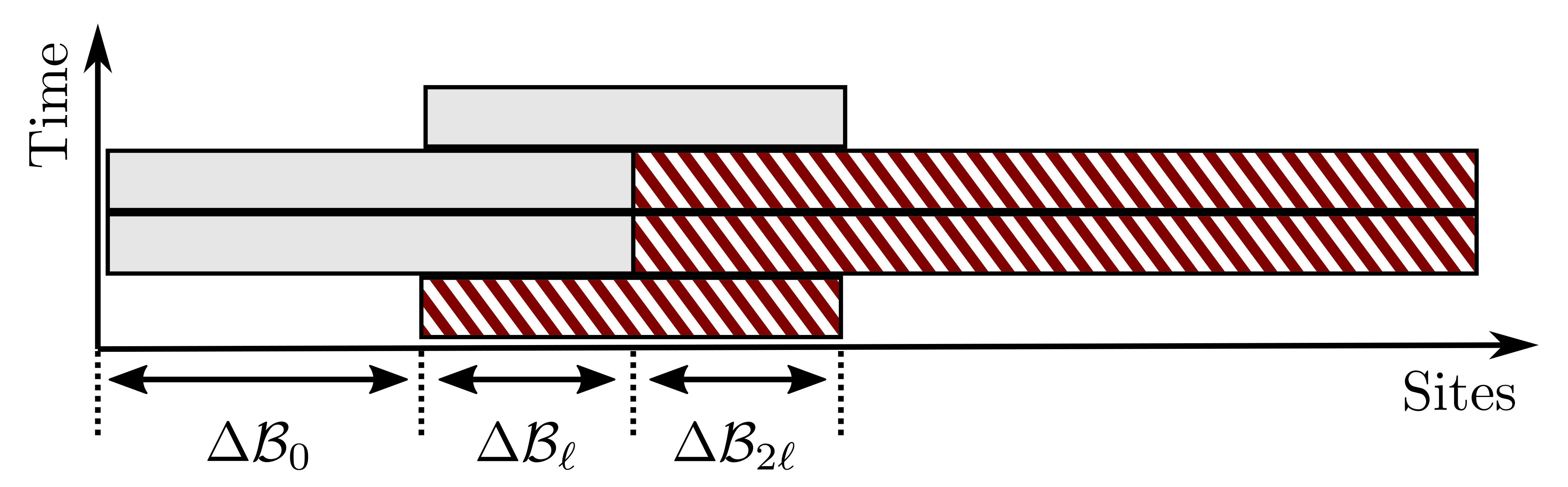
Figure 1: Demonstration of the second-order product formula for simulating the evolution of an observable $B$ supported on $\mathcal{S}(B)=\Delta\mathcal{B}_{0}$. Each rectangle represents a unitary supported on the sites covered by the width of the rectangle. The evolution unitary $e^{-itH}$ is decomposed using the second-order product formula into $\Upsilon=2$ stages. Each stage is a sequence of $\Gamma=3$ matrix exponentials generated by Hamiltonian terms supported on parts of the system. Some of these unitaries (red shaded rectangles) can subsequently be commuted through $B$ in the expression $\mathscr{S}_{\text{trunc}}^{\dagger}(t)B\mathscr{S}_{\text{trunc}}(t)$ to cancel out with their Hermitian conjugates. As a result, the time-evolved version of $B$ can be effectively described by the remaining unitaries (light-gray rectangles).

Starting from the power-law Hamiltonian $H=\sum_{\vec{i},\vec{j}\in\Lambda}H_{\vec{i},\vec{j}}$, we group terms based on their distance to the observable $B$ and define

$$H_{1}=\sum_{\vec{i},\vec{j}\in\mathcal{B}_{\ell}}H_{\vec{i},\vec{j}},$$ (79)

$$H_{\gamma}=\sum_{\vec{i},\vec{j}\in\Delta\mathcal{B}_{\gamma\ell}}H_{\vec{i},\vec{j}}+\sum_{\begin{subarray}{c}\vec{i}\in\Delta\mathcal{B}_{(\gamma-1)\ell}\\ \vec{j}\in\Delta\mathcal{B}_{\gamma\ell}\end{subarray}}H_{\vec{i},\vec{j}}\quad\text{ for }\gamma=2,\dots,\Gamma-1,$$ (80)

$$H_{\Gamma}=\sum_{\vec{i},\vec{j}\notin\mathcal{B}_{(\Gamma-2)\ell}}H_{\vec{i},\vec{j}}$$ (81)

with constant $\Gamma$ to be chosen later. In this construction, all $H_{\gamma}$ with even $\gamma$ commute and all $H_{\gamma}$ with odd $\gamma$ commute. We consider the truncated Hamiltonian

$$H_{\text{trunc}}=\sum_{\gamma=1}^{\Gamma}H_{\gamma}$$ (82)

instead of $H$, which incurs a truncation error of

$$\epsilon_{1}=\mathcal{O}\mathopen{}\mathclose{{}\left(\mathopen{}\mathclose{{}\left\lVert e^{-itH}-e^{-itH_{\text{trunc}}}}\right\rVert}\right)=\mathcal{O}\mathopen{}\mathclose{{}\left(\mathopen{}\mathclose{{}\left\lVert H-H_{\text{trunc}}}\right\rVert t}\right)=\mathcal{O}\mathopen{}\mathclose{{}\left(\frac{(y_{0}+\Gamma\ell)^{d-1}t}{\ell^{\alpha-d-1}}}\right).$$ (83)

See Appendix H for proof details.

Next, we simulate the evolution $e^{-itH_{\text{trunc}}}$ using the $p$th-order product formula [See Eq. 15 and Fig. 1]:

$$\mathscr{S}_{\text{trunc}}(t)=\prod_{\upsilon=1}^{\Upsilon}\prod_{\gamma=1}^{\Gamma}e^{-ita_{(\upsilon,\gamma)}H_{\pi_{\upsilon}(\gamma)}},$$ (84)

where we put additional constraints on the permutation $\pi_{\nu}$:

$$\pi_{\upsilon}(1,2,3,4,5,6,\ldots)=\begin{cases}(2,4,6,\dots,1,3,5,\dots),\quad&\text{ if }\upsilon\text{ is odd},\\ (1,3,5,\dots,2,4,6,\dots),&\text{ if }\upsilon\text{ is even}.\end{cases}$$ (85)

Such a permutation can be realized using Suzuki’s original construction [84] and taking into account that $\mathopen{}\mathclose{{}\left[H_{2k},H_{2k^{\prime}}}\right]=0$ and $\mathopen{}\mathclose{{}\left[H_{2k+1},H_{2k^{\prime}+1}}\right]=0$ for all $k,k^{\prime}$. Using Theorem 11, we show in Appendix H that the error of approximating $e^{-itH_{\text{trunc}}}$ by $\mathscr{S}_{\text{trunc}}(t)$ is

$$\epsilon_{2} =\mathopen{}\mathclose{{}\left\lVert e^{-itH_{\text{trunc}}}-\mathscr{S}_{\text{trunc}}(t)}\right\rVert$$

$$=\mathcal{O}\mathopen{}\mathclose{{}\left(\sum_{\gamma_{1},\dots,\gamma_{p+1}=1}^{\Gamma}\mathopen{}\mathclose{{}\left\lVert\mathopen{}\mathclose{{}\left[H_{\gamma_{p+1}},\dots,\mathopen{}\mathclose{{}\left[H_{\gamma_{2}},H_{\gamma_{1}}}\right]}\right]}\right\rVert t^{p+1}}\right)=\mathcal{O}\mathopen{}\mathclose{{}\left((y_{0}+\Gamma\ell)^{d-1}\ell t^{p+1}}\right).$$ (86)

Note that the Hamiltonian terms $H_{\gamma}$ (for $\gamma\geq 2$) commute with $B$. Therefore, the exponentials in $\mathscr{S}_{\text{trunc}}(t)$ corresponding to these terms can be commuted through $B$ to cancel with their counterparts in $\mathscr{S}_{\text{trunc}}(t)^{\dagger}$. By choosing the constant $\Gamma=\Upsilon+1$, we have

$$\mathscr{S}_{\text{trunc}}^{\dagger}(t)B\mathscr{S}_{\text{trunc}}(t)=\mathscr{S}_{\text{reduce}}^{\dagger}(t)B\mathscr{S}_{\text{reduce}}(t),$$ (87)

where

$$\mathscr{S}_{\text{reduce}}(t)=\prod_{\upsilon=1}^{\Upsilon}\prod_{\gamma=1}^{\upsilon}e^{-ita_{(\upsilon,\pi_{\upsilon}^{-1}(\gamma))}H_{\gamma}}.$$ (88)

We call $\mathscr{S}_{\text{reduce}}(t)$ the reduced product formula. This approximates the evolution $e^{-itH}$ of local observable $B$ with error

$$\mathopen{}\mathclose{{}\left\lVert e^{itH}Be^{-itH}-\mathscr{S}_{\text{reduce}}^{\dagger}(t)B\mathscr{S}_{\text{reduce}}(t)}\right\rVert \leq\mathopen{}\mathclose{{}\left\lVert e^{itH}Be^{-itH}-e^{itH_{\text{trunc}}}Be^{-itH_{\text{trunc}}}}\right\rVert$$ (89)

$$\quad+\mathopen{}\mathclose{{}\left\lVert e^{itH_{\text{trunc}}}Be^{-itH_{\text{trunc}}}-\mathscr{S}_{\text{trunc}}^{\dagger}(t)B\mathscr{S}_{\text{trunc}}(t)}\right\rVert$$

$$\quad+\mathopen{}\mathclose{{}\left\lVert\mathscr{S}_{\text{trunc}}^{\dagger}(t)B\mathscr{S}_{\text{trunc}}(t)-\mathscr{S}_{\text{reduce}}^{\dagger}(t)B\mathscr{S}_{\text{reduce}}(t)}\right\rVert$$

$$\leq 2\mathopen{}\mathclose{{}\left\lVert B}\right\rVert(\epsilon_{1}+\epsilon_{2})+0$$

$$=\mathcal{O}\mathopen{}\mathclose{{}\left(\mathopen{}\mathclose{{}\left\lVert B}\right\rVert t(y_{0}+\Gamma\ell)^{d-1}\mathopen{}\mathclose{{}\left(\frac{1}{\ell^{\alpha-d-1}}+\ell t^{p}}\right)}\right).$$

The above decomposition is accurate for a short-time evolution. For larger times, we divide the simulation into $r$ Trotter steps and apply this decomposition within each step. We analyze the error in a similar way as above, except that $B$ is defined by applying the reduced product formula to the observable $A$. Since the spectral norm is invariant under unitary transformations, we have $\mathopen{}\mathclose{{}\left\lVert B}\right\rVert=\mathopen{}\mathclose{{}\left\lVert A}\right\rVert=\mathcal{O}\mathopen{}\mathclose{{}\left(1}\right)$. Another difference is that the support of the observable is expanded by $\Gamma\ell$ after each Trotter step; i.e., we set $y_{0}$ to be $x_{0}$, $x_{0}+\Gamma\ell$,…, and $x_{0}+r\Gamma\ell$. Using the triangle inequality, we bound the error of the reduced product formula by

$$\mathcal{O}\mathopen{}\mathclose{{}\left(t(x_{0}+r\Gamma\ell)^{d-1}\mathopen{}\mathclose{{}\left(\frac{1}{\ell^{\alpha-d-1}}+\ell\frac{t^{p}}{r^{p}}}\right)}\right).$$ (90)

We now apply the above procedure in the reverse direction, but only to Hamiltonian terms within the light cone, incurring a truncation error at most $\epsilon_{1}$ and a Trotter error at most $\epsilon_{2}$. This replaces $\mathscr{S}_{\text{reduce}}(t)$ by $\mathscr{S}_{\text{lc}}(t)$, the product formula that simulates the Hamiltonian $H_{\text{lc}}$ whose terms have distance at most $r\Gamma\ell$ to the local observable $A$. See Figure 2 for a step-by-step illustration of this approach. We analyze the error in a similar way as above, establishing the following result on evolving local observables.

Figure 2: Construction of the Hamiltonian $H_{\text{lc}}$ within the light cone such that $e^{itH}Ae^{-itH}\approx e^{itH_{\text{lc}}}Ae^{-itH_{\text{lc}}}$. Each rectangle represents a unitary supported on the sites covered by the width of the rectangle. Specifically, the rectangle in the top-left panel represents the evolution $e^{-itH}$ that we want to decompose. We divide the evolution into $r$ steps. Within each step, we truncate the Hamiltonian to $H_{\text{trunc}}$ and decompose its evolution using a product formula $\mathscr{S}_{\text{trunc}}$. We commute certain matrix exponentials in $\mathscr{S}_{\text{trunc}}$ (represented by red shaded rectangles) through the observable to cancel their counterpart, obtaining $\mathscr{S}_{\text{reduce}}$ in the top-right panel. We reverse this procedure within the light cone to construct $\mathscr{S}_{\text{lc}}$ in the bottom-right panel, which approximates $e^{-itH_{\text{lc}}}$ as illustrated in the bottom-left panel.

Proposition 13 (Product-formula decomposition of evolutions of local observables).

Let $\Lambda\subseteq\mathbb{R}^{d}$ be a $d$-dimensional square lattice. Let $H$ be a power-law Hamiltonian (66) with exponent $\alpha>2d$ and $A$ be an observable with support enclosed in a $d$-dimensional ball of constant radius $x_{0}$. Construct the Hamiltonian $H_{\text{lc}}$ as above using $p$th-order $\Upsilon$-stage product formulas $\mathscr{S}_{\text{trunc}}(t)$, $\mathscr{S}_{\text{reduce}}(t)$, and $\mathscr{S}_{\text{lc}}(t)$. Then, the support of $H_{\text{lc}}$ has radius $x_{0}+r\Gamma\ell$ and

$$\mathopen{}\mathclose{{}\left\lVert e^{itH}Ae^{-itH}-e^{itH_{\text{lc}}}Ae^{-itH_{\text{lc}}}}\right\rVert =\mathcal{O}\mathopen{}\mathclose{{}\left(t(x_{0}+r\Gamma\ell)^{d-1}\mathopen{}\mathclose{{}\left(\frac{1}{\ell^{\alpha-d-1}}+\ell\frac{t^{p}}{r^{p}}}\right)}\right),$$ (91)

where the positive integer $\ell$ is a parameter and $\Gamma=\Upsilon+1$ is constant.

Gate complexity of simulating local observables. We now analyze the gate complexity of simulating local observables using the decomposition in Proposition 13. Assuming the support $\mathcal{S}(A)$ has constant radius $x_{0}=\mathcal{O}\mathopen{}\mathclose{{}\left(1}\right)$ and $\Gamma=\mathcal{O}\mathopen{}\mathclose{{}\left(1}\right)$, we simplify the error bound in (91) to

$$\mathopen{}\mathclose{{}\left\lVert e^{itH}Ae^{-itH}-e^{itH_{\text{lc}}}Ae^{-itH_{\text{lc}}}}\right\rVert=\mathcal{O}\mathopen{}\mathclose{{}\left(t(r\ell)^{d-1}\mathopen{}\mathclose{{}\left(\frac{1}{\ell^{\alpha-d-1}}+\frac{\ell t^{p}}{r^{p}}}\right)}\right).$$ (92)

To minimize the error, we choose the cutoff $\ell=\Theta\mathopen{}\mathclose{{}\left(\mathopen{}\mathclose{{}\left(\frac{r}{t}}\right)^{\frac{p}{\alpha-d}}}\right)$, which is larger than $1$ provided $r\geq t$ (and recall that we assume $\alpha>2d$, so in particular, $\alpha>d$). With this choice of $\ell$, the error becomes

$$\mathcal{O}\mathopen{}\mathclose{{}\left(tr^{d-1}\mathopen{}\mathclose{{}\left(\frac{t}{r}}\right)^{\frac{p(\alpha-2d)}{\alpha-d}}}\right)=\mathcal{O}\mathopen{}\mathclose{{}\left(\frac{t^{\frac{p(\alpha-2d)+\alpha-d}{\alpha-d}}}{r^{\frac{p(\alpha-2d)-(\alpha-d)(d-1)}{\alpha-d}}}}\right).$$ (93)

We then choose an appropriate Trotter number $r$ as detailed in Appendix H and find that

$$g_{\alpha}={t^{\mathopen{}\mathclose{{}\left(1+d\frac{\alpha-d}{\alpha-2d}}\right)\mathopen{}\mathclose{{}\left(1+\frac{d}{\alpha-d}}\right)+o(1)}}$$ (94)

gates suffice to simulate a local observable with constant accuracy. The gate count is independent of the system size and thus less than the cost of simulating the full dynamics (69) when the system size is $n=\Omega\mathopen{}\mathclose{{}\left(t^{d(\alpha-d)/(\alpha-2d)}}\right)$. However, in contrast to the simulation of $e^{-itH}$ where the asymptotic error scaling is robust against the reordering of Hamiltonian terms, we obtain a smaller error for simulating $\mathscr{A}(t)$ by defining product formulas with a special ordering that preserves the locality of the simulated system.

Additionally, in the limit $\alpha\rightarrow\infty$ which corresponds to nearest-neighbor interactions, we have the gate count

$$g_{\infty}={t^{d+1+o(1)}}.$$ (95)

This has a clear physical intuition: it is (nearly) proportional to the space-time volume $t^{d+1}$ inside a linear light cone generated by the evolution.

Lieb-Robinson-type bound for power-law Hamiltonians. The Lieb-Robinson bounds—first derived for nearest-neighbor interactions [58] and subsequently generalized to power-law systems [43, 70, 71, 37, 36, 81, 87, 21]—have found numerous applications in physics, including designing new algorithms for quantum simulations [38, 87]. They bound the speed at which a local disturbance spreads in quantum systems. Here, we show that the decomposition of Proposition 13 constructed using product formulas also implies a Lieb-Robinson-type bound for power-law Hamiltonians.

The subject of the Lieb-Robinson bounds is usually the commutator norm

$$\mathcal{C}(t,\rho)=\mathopen{}\mathclose{{}\left\lVert\mathopen{}\mathclose{{}\left[e^{itH}Ae^{-itH},B}\right]}\right\rVert,$$ (96)

where $A,B$ are two operators whose supports have distance

$$\textrm{dist}(\mathcal{S}(A),\mathcal{S}(B))=\inf\limits_{\vec{i}\in\mathcal{S}(A),\vec{j}\in\mathcal{S}(B)}\mathopen{}\mathclose{{}\left\lVert\vec{i}-\vec{j}}\right\rVert_{2}=\rho$$ (97)

and $e^{-itH}$ is the time evolution unitary generated by a power-law Hamiltonian $H$. Our above discussion shows that $e^{itH}Ae^{-itH}$ is approximately $e^{itH_{\text{lc}}}Ae^{-itH_{\text{lc}}}$, which is supported on a ball of radius $x=\mathcal{O}\mathopen{}\mathclose{{}\left(r\ell}\right)=\mathcal{O}\mathopen{}\mathclose{{}\left(r\mathopen{}\mathclose{{}\left(r/t}\right)^{\frac{p}{\alpha-d}}}\right)$ centered on $\mathcal{S}(A)$. By choosing $r=\Theta\mathopen{}\mathclose{{}\left({\rho^{\frac{\alpha-d}{\alpha-d+p}}}{t^{\frac{p}{\alpha-d+p}}}}\right)$ so that $x<\rho$, we make $e^{itH_{\text{lc}}}Ae^{-itH_{\text{lc}}}$ commute with $B$ and therefore $\mathcal{C}(t,\rho)$ is small. More precisely,

$$\mathcal{C}(t,r)=\mathcal{O}\mathopen{}\mathclose{{}\left(\frac{t^{\frac{p(\alpha-2d)+\alpha-d}{\alpha-d}}}{r^{\frac{p(\alpha-2d)-(\alpha-d)(d-1)}{\alpha-d}}}}\right)=\mathcal{O}\mathopen{}\mathclose{{}\left(\frac{t^{\frac{(p+1)(\alpha-d)}{\alpha-d+p}}}{\rho^{\frac{p(\alpha-2d)-(\alpha-d)(d-1)}{\alpha-d+p}}}}\right)={\frac{t^{\alpha-d+o(1)}}{\rho^{\alpha-2d+o(1)}}}.$$ (98)

Note that we have implicitly assumed that $\rho^{\frac{\alpha-d}{\alpha-d+p}}t^{\frac{p}{\alpha-d+p}}\geq 1$ so that we can choose $r\geq 1$. The bound implies a light cone $t\gtrsim\rho^{\frac{\alpha-2d}{\alpha-d}+o(1)}$, which can be made arbitrarily close to the light cone $t\gtrsim\rho^{\frac{\alpha-2d}{\alpha-d}}$ of the recent bound in Ref. [87] for all values of $d$.

4.3 Applications to quantum Monte Carlo simulation

We now apply our result to improving the performance of quantum Monte Carlo simulation. Here, the goal is to approximate certain properties of the Hamiltonian, such as the partition function, rather than simulating the full dynamics. We consider two specific systems: the transverse field Ising model of [17] and the ferromagnetic quantum spin systems of [18]. For both simulations, the ideal evolution is decomposed using the second-order Suzuki formula and we show that such a decomposition can be made more efficient using our tightened analysis.

Transverse field Ising model. Consider the following $n$-qubit transverse field Ising model:

$$H=-A-B,\quad A=\sum_{1\leq u<v\leq n}j_{u,v}Z_{u}Z_{v},\quad B=\sum_{1\leq u\leq n}h_{u}X_{u}.$$ (99)

Here, $X_{u}$ and $Z_{u}$ are Pauli operators acting on the $u$th qubit, and $j_{u,v}\geq 0$ and $h_{u}\geq 0$ are nonnegative coefficients. Define $j:=\max\{j_{u,v},h_{u}\}$ to be the maximum norm of the interactions. Our goal is to approximate the partition function

$$\mathcal{Z}=\mathrm{Tr}\big{(}e^{-H}\big{)}$$ (100)

up to a multiplicative error $0<\epsilon<1$.

Reference [17] solves this problem with an efficient classical algorithm. A key step in their algorithm is a decomposition of the evolution operator using the second-order Suzuki formula, so that

$$\mathcal{Z}^{\prime}=\mathrm{Tr}\big{(}e^{\frac{1}{2r}A}e^{\frac{1}{r}B}e^{\frac{1}{2r}A}\big{)}^{r}\lessapprox(1+\epsilon)\mathrm{Tr}\big{(}e^{-H}\big{)}=(1+\epsilon)\mathcal{Z}.$$ (101)

However, their original analysis does not exploit the commutativity relation between $A$ and $B$, and can be improved by the techniques developed here.

Note that this is different from the usual setting of digital quantum simulation. Indeed, as the matrix exponentials in the product formula are no longer unitary, we will introduce an additional multiplicative factor when we apply Theorem 11. Also, we need to estimate the multiplicative error as opposed to the additive error of the Trotter decomposition, which is addressed by the following lemma.

Lemma 14 (Relative perturbation of eigenvalues [31, Theorem 2.1] [48, Theorem 5.4]).

Let matrix $C$ be positive semidefinite and $D$ be nonsingular. Assume that the eigenvalues $\lambda_{i}(C)$ and $\lambda_{i}(D^{\dagger}CD)$ are ordered nonincreasingly. Then,

$$\lambda_{i}(D^{\dagger}CD)\leq\lambda_{i}(C)\mathopen{}\mathclose{{}\left\lVert D^{\dagger}D}\right\rVert.$$ (102)

Let $A$ and $B$ be Hermitian matrices and consider the evolution $e^{t(A+B)}$ with $t\geq 0$. Our goal is to choose $r$ sufficiently large so that the eigenvalues are approximated as

$$\lambda_{i}\Big{(}\big{(}e^{\frac{t}{2r}A}e^{\frac{t}{r}B}e^{\frac{t}{2r}A}\big{)}^{r}\Big{)}\approx\lambda_{i}\Big{(}e^{t(A+B)}\Big{)}$$ (103)

up to a small multiplicative error. We define

$$U :=e^{\frac{t}{r}(A+B)},$$ (104)

$$V :=e^{\frac{t}{2r}A}e^{\frac{t}{r}B}e^{\frac{t}{2r}A},$$

$$W :=\exp_{\mathcal{T}}\bigg{(}\int_{0}^{\frac{t}{r}}\mathrm{d}\tau\ e^{-\tau(A+B)}\bigg{[}e^{\frac{\tau}{2}A}Be^{-\frac{\tau}{2}A}-B+e^{\frac{\tau}{2}A}e^{\tau B}\frac{A}{2}e^{-\tau B}e^{-\frac{\tau}{2}A}-\frac{A}{2}\bigg{]}e^{\tau(A+B)}\bigg{)}.$$

Then, both $U$ and $V$ are positive-semidefinite operators and we know from Theorem 8 that $V=UW$. In Appendix I, we show that

$$\mathopen{}\mathclose{{}\left\lVert W}\right\rVert\leq\exp\bigg{(}\bigg{(}\frac{t^{3}}{8r^{3}}\mathopen{}\mathclose{{}\left\lVert\big{[}A,\big{[}A,B\big{]}\big{]}}\right\rVert+\frac{t^{3}}{12r^{3}}\mathopen{}\mathclose{{}\left\lVert\big{[}B,\big{[}B,A\big{]}\big{]}}\right\rVert\bigg{)}e^{4\frac{t}{r}(\mathopen{}\mathclose{{}\left\lVert A}\right\rVert+\mathopen{}\mathclose{{}\left\lVert B}\right\rVert)}\bigg{)}.$$ (105)

Our goal is to bound the eigenvalues $\lambda_{i}\big{(}V^{r}\big{)}$ in terms of $\lambda_{i}\big{(}U^{r}\big{)}$. This can be done recursively as follows. We first replace the rightmost $V$ by $UW$ and the leftmost $V$ by $W^{\dagger}U$. Invoking Lemma 14, we have

$$\lambda_{i}\big{(}V^{r}\big{)}=\lambda_{i}\big{(}W^{\dagger}UV^{r-2}UW\big{)}\leq\lambda_{i}\big{(}UV^{r-2}U\big{)}\mathopen{}\mathclose{{}\left\lVert W}\right\rVert^{2}.$$ (106)

By [46, Theorem 1.3.22],

$$\lambda_{i}\big{(}UV^{r-2}U\big{)}=\lambda_{i}\big{(}V^{\frac{r}{2}-1}UUV^{\frac{r}{2}-1}\big{)}.$$ (107)

We now apply a similar procedure to obtain

$$\lambda_{i}\big{(}V^{\frac{r}{2}-1}UUV^{\frac{r}{2}-1}\big{)} =\lambda_{i}\big{(}W^{\dagger}UV^{\frac{r}{2}-2}UUV^{\frac{r}{2}-2}UW\big{)}$$ (108)

$$\leq\lambda_{i}\big{(}UV^{\frac{r}{2}-2}UUV^{\frac{r}{2}-2}U\big{)}\mathopen{}\mathclose{{}\left\lVert W}\right\rVert^{2}$$

$$=\lambda_{i}\big{(}V^{\frac{r}{4}-1}UUV^{\frac{r}{2}-2}UUV^{\frac{r}{4}-1}\big{)}\mathopen{}\mathclose{{}\left\lVert W}\right\rVert^{2}$$

$$\leq\lambda_{i}\big{(}UV^{\frac{r}{4}-2}UUV^{\frac{r}{2}-2}UUV^{\frac{r}{4}-2}U\big{)}\mathopen{}\mathclose{{}\left\lVert W}\right\rVert^{4}$$

$$=\lambda_{i}\big{(}V^{\frac{r}{4}-1}UUV^{\frac{r}{4}-2}UUV^{\frac{r}{4}-2}UUV^{\frac{r}{4}-1}\big{)}\mathopen{}\mathclose{{}\left\lVert W}\right\rVert^{4}$$

$$\leq\lambda_{i}\big{(}UV^{\frac{r}{4}-2}UUV^{\frac{r}{4}-2}UUV^{\frac{r}{4}-2}UUV^{\frac{r}{4}-2}U\big{)}\mathopen{}\mathclose{{}\left\lVert W}\right\rVert^{6}.$$

To ensure that this recursion is valid, we choose $r$ to be a power of $2$. Since any positive integer is between $2^{m}$ and $2^{m+1}$ for some $m\geq 0$, this choice only enlarges $r$ by a factor of at most $2$. Overall,

$$\lambda_{i}\big{(}V^{r}\big{)}\leq\lambda_{i}\big{(}U^{r}\big{)}\mathopen{}\mathclose{{}\left\lVert W}\right\rVert^{r}.$$ (109)

We know that

$$\mathopen{}\mathclose{{}\left\lVert W}\right\rVert^{r}\leq\exp\bigg{(}\bigg{(}\frac{t^{3}}{8r^{2}}\mathopen{}\mathclose{{}\left\lVert\big{[}A,\big{[}A,B\big{]}\big{]}}\right\rVert+\frac{t^{3}}{12r^{2}}\mathopen{}\mathclose{{}\left\lVert\big{[}B,\big{[}B,A\big{]}\big{]}}\right\rVert\bigg{)}e^{4\frac{t}{r}(\mathopen{}\mathclose{{}\left\lVert A}\right\rVert+\mathopen{}\mathclose{{}\left\lVert B}\right\rVert)}\bigg{)}.$$ (110)

We first choose

$$r\geq 4t\big{(}\mathopen{}\mathclose{{}\left\lVert A}\right\rVert+\mathopen{}\mathclose{{}\left\lVert B}\right\rVert\big{)}$$ (111)

so that $e^{4\frac{t}{r}(\mathopen{}\mathclose{{}\left\lVert A}\right\rVert+\mathopen{}\mathclose{{}\left\lVert B}\right\rVert)}\leq e<4$. We then set

$$r\geq\max\bigg{\{}\sqrt{\frac{t^{3}}{\epsilon}\mathopen{}\mathclose{{}\left\lVert\big{[}A,\big{[}A,B\big{]}\big{]}}\right\rVert},\sqrt{\frac{2t^{3}}{3\epsilon}\mathopen{}\mathclose{{}\left\lVert\big{[}B,\big{[}B,A\big{]}\big{]}}\right\rVert}\bigg{\}}$$ (112)

so that both $\frac{t^{3}}{8r^{2}}\mathopen{}\mathclose{{}\left\lVert\big{[}A,\big{[}A,B\big{]}\big{]}}\right\rVert$ and $\frac{t^{3}}{12r^{2}}\mathopen{}\mathclose{{}\left\lVert\big{[}B,\big{[}B,A\big{]}\big{]}}\right\rVert$ are bounded by $\epsilon/8$. Therefore, we have $\mathopen{}\mathclose{{}\left\lVert W}\right\rVert^{r}\leq e^{\epsilon}$ as long as $r$ is a power of $2$ satisfying

$$r\geq\max\bigg{\{}4t\big{(}\mathopen{}\mathclose{{}\left\lVert A}\right\rVert+\mathopen{}\mathclose{{}\left\lVert B}\right\rVert\big{)},\sqrt{\frac{t^{3}}{\epsilon}\mathopen{}\mathclose{{}\left\lVert\big{[}A,\big{[}A,B\big{]}\big{]}}\right\rVert},\sqrt{\frac{2t^{3}}{3\epsilon}\mathopen{}\mathclose{{}\left\lVert\big{[}B,\big{[}B,A\big{]}\big{]}}\right\rVert}\bigg{\}},$$ (113)

which implies

$$\mathcal{Z}^{\prime}=\sum_{i}\lambda_{i}\big{(}V^{r}\big{)}\leq\sum_{i}\lambda_{i}\big{(}U^{r}\big{)}e^{\epsilon}\approx(1+\epsilon)\sum_{i}\lambda_{i}\big{(}U^{r}\big{)}=(1+\epsilon)\mathcal{Z}$$ (114)

assuming $\epsilon\ll 1$.

Following similar arguments, we can show that this choice of $r$ also gives a lower bound of $\mathcal{Z}^{\prime}$ with $\mathcal{Z}^{\prime}\gtrapprox(1-\epsilon)\mathcal{Z}$. Indeed, we can bound the eigenvalues $\lambda_{i}\big{(}U^{r}\big{)}$ in terms of $\lambda_{i}\big{(}V^{r}\big{)}$ using Lemma 14 and the relation $U=VW^{-1}$. Using Lemma 4 and the fact that $W^{-1}$ is the reversal of the time-ordered exponential $W$, we have $\mathopen{}\mathclose{{}\left\lVert W^{-1}}\right\rVert^{r}\leq e^{\epsilon}$ as well, giving $\sum_{i}\lambda_{i}\big{(}U^{r}\big{)}\leq\sum_{i}\lambda_{i}\big{(}V^{r}\big{)}e^{\epsilon}$. The lower bound now follows since $1/e^{\epsilon}\approx 1/(1+\epsilon)\approx 1-\epsilon$ for $\epsilon\ll 1$. We have therefore approximated the partition function up to a multiplicative error $\epsilon$.

We now specialize our result to the transverse field Ising Hamiltonian with $t=1$. We find that

$$\mathopen{}\mathclose{{}\left\lVert A}\right\rVert=\mathcal{O}\mathopen{}\mathclose{{}\left(n^{2}j}\right),\quad\mathopen{}\mathclose{{}\left\lVert B}\right\rVert=\mathcal{O}\mathopen{}\mathclose{{}\left(nj}\right),\quad\mathopen{}\mathclose{{}\left\lVert\big{[}A,\big{[}A,B\big{]}\big{]}}\right\rVert=\mathcal{O}\mathopen{}\mathclose{{}\left(n^{3}j^{3}}\right),\quad\mathopen{}\mathclose{{}\left\lVert\big{[}B,\big{[}B,A\big{]}\big{]}}\right\rVert=\mathcal{O}\mathopen{}\mathclose{{}\left(n^{2}j^{3}}\right),$$ (115)

which implies

$$r=\mathcal{O}\mathopen{}\mathclose{{}\left(n^{2}j+n^{3/2}j^{3/2}\epsilon^{-1/2}}\right).$$ (116)

By [17, p. 17], this gives a fully polynomial randomized approximation scheme (FPRAS) with running time

$$\widetilde{\mathcal{O}}\mathopen{}\mathclose{{}\left(n^{17}r^{14}\epsilon^{-2}}\right)=\widetilde{\mathcal{O}}\mathopen{}\mathclose{{}\left(n^{45}j^{14}\epsilon^{-2}+n^{38}j^{21}\epsilon^{-9}}\right),$$ (117)

improving over the previous complexity of

$$\widetilde{\mathcal{O}}\mathopen{}\mathclose{{}\left(n^{59}j^{21}\epsilon^{-9}}\right).$$ (118)

Quantum ferromagnets. We now apply our technique to improve the Monte Carlo simulation of ferromagnetic quantum spin systems [18]. Such systems are described by the $n$-qubit Hamiltonian

$$H=\sum_{1\leq u<v\leq n}\big{(}{-}b_{uv}X_{u}X_{v}+c_{uv}Y_{u}Y_{v}\big{)}+\sum_{u=1}^{n}d_{u}\big{(}I+Z_{u}\big{)},$$ (119)

where $0\leq b_{uv}\leq 1$, $-b_{uv}\leq c_{uv}\leq b_{uv}$, and $-1\leq d_{uv}\leq 1$. It will be convenient to rewrite these Hamiltonians using the coefficients $p_{uv}=(b_{uv}-c_{uv})/2$ and $q_{uv}=(b_{uv}+c_{uv})/2$ as

$$H=\sum_{1\leq u<v\leq n}p_{uv}\big{(}{-}X_{u}X_{v}-Y_{u}Y_{v}\big{)}+\sum_{1\leq u<v\leq n}q_{uv}\big{(}{-}X_{u}X_{v}+Y_{u}Y_{v}\big{)}+\sum_{u=1}^{n}d_{u}\big{(}I+Z_{u}\big{)}.$$ (120)

Since $|c_{uv}|\leq b_{uv}\leq 1$, we have $p_{uv},q_{uv}\in[0,1]$.

Our goal is to approximate the partition function

$$\mathcal{Z}(\beta,H)=\mathrm{Tr}\big{[}e^{-\beta H}\big{]}$$ (121)

for $\beta>0$. Following the setting of [18], we restrict ourselves to the $n$-qubit matchgate set

$$\bigg{\{}f_{u}\big{(}e^{\pm t}\big{)},g_{uv}(t),h_{uv}(t)\ \bigg{|}\ u,v=1,\ldots,n,\ u\neq v,\ 0<t<\frac{1}{2}\bigg{\}},$$ (122)

where

$$f\big{(}e^{\pm t}\big{)}=\begin{bmatrix}e^{\pm t}&0\\ 0&1\end{bmatrix},\qquad g(t)=\begin{bmatrix}1+t^{2}&0&0&t\\ 0&1&0&0\\ 0&0&1&0\\ t&0&0&1\end{bmatrix},\qquad h(t)=\begin{bmatrix}1&0&0&0\\ 0&1+t^{2}&t&0\\ 0&t&1&0\\ 0&0&0&1\end{bmatrix}$$ (123)

and the subscripts $u,v$ indicate the qubits on which the gates act nontrivially. The motivations for using these gates can be found in [18] which we do not repeat here. These gates approximately implement the exponential of the Hamiltonian terms in the sense that

$$f_{u}\big{(}e^{\pm t}\big{)}=e^{\pm\frac{t}{2}(I+Z_{u})},\qquad g_{uv}(t)=e^{-\frac{t}{2}(-X_{u}X_{v}+Y_{u}Y_{v})+O\mathopen{}\mathclose{{}\left(t^{2}}\right)},\qquad h_{uv}(t)=e^{-\frac{t}{2}(-X_{u}X_{v}-Y_{u}Y_{v})+O\mathopen{}\mathclose{{}\left(t^{2}}\right)}.$$ (124)

We divide the evolution into $r$ steps and apply the second-order Suzuki formula within each step, obtaining

$$e^{-\frac{\beta}{r}H} \approx\prod_{1\leq u\leq n}e^{-\frac{\beta}{2r}d_{u}(I+Z_{u})}\prod_{1\leq u<v\leq n}e^{-\frac{\beta}{2r}q_{uv}({-}X_{u}X_{v}+Y_{u}Y_{v})}\prod_{1\leq u<v\leq n}e^{-\frac{\beta}{2r}p_{uv}({-}X_{u}X_{v}-Y_{u}Y_{v})}$$ (125)

$$\quad\cdot\prod_{1\leq u<v\leq n}e^{-\frac{\beta}{2r}p_{uv}({-}X_{u}X_{v}-Y_{u}Y_{v})}\prod_{1\leq u<v\leq n}e^{-\frac{\beta}{2r}q_{uv}({-}X_{u}X_{v}+Y_{u}Y_{v})}\prod_{1\leq u\leq n}e^{-\frac{\beta}{2r}d_{u}(I+Z_{u})}$$

$$\approx\prod_{1\leq u\leq n}f_{u}\big{(}e^{-\frac{\beta}{r}d_{u}}\big{)}\prod_{1\leq u<v\leq n}g_{uv}\bigg{(}\frac{\beta}{r}q_{uv}\bigg{)}\prod_{1\leq u<v\leq n}h_{uv}\bigg{(}\frac{\beta}{r}p_{uv}\bigg{)}$$

$$\quad\cdot\prod_{1\leq u<v\leq n}h_{uv}\bigg{(}\frac{\beta}{r}p_{uv}\bigg{)}\prod_{1\leq u<v\leq n}g_{uv}\bigg{(}\frac{\beta}{r}q_{uv}\bigg{)}\prod_{1\leq u\leq n}f_{u}\big{(}e^{-\frac{\beta}{r}d_{u}}\big{)}.$$

Here, we have two sources of error: the Trotter error and the error from using the gate set (122). We choose

$$r>2\beta,$$ (126)

so that we can implement the product formula using gates from (122) with parameters

$$-\frac{1}{2}<-\frac{\beta}{r}d_{u}<\frac{1}{2},\quad 0<\frac{\beta}{r}q_{uv}<\frac{1}{2},\quad 0<\frac{\beta}{r}p_{uv}<\frac{1}{2}.$$ (127)

In Appendix I, we use the interaction picture (Lemma 2) to show that

$$\prod_{1\leq u\leq n}f_{u}\big{(}e^{-\frac{\beta}{r}d_{u}}\big{)}\prod_{1\leq u<v\leq n}g_{uv}\bigg{(}\frac{\beta}{r}q_{uv}\bigg{)}\prod_{1\leq u<v\leq n}h_{uv}\bigg{(}\frac{\beta}{r}p_{uv}\bigg{)}$$ (128)

$$\quad\cdot\prod_{1\leq u<v\leq n}h_{uv}\bigg{(}\frac{\beta}{r}p_{uv}\bigg{)}\prod_{1\leq u<v\leq n}g_{uv}\bigg{(}\frac{\beta}{r}q_{uv}\bigg{)}\prod_{1\leq u\leq n}f_{u}\big{(}e^{-\frac{\beta}{r}d_{u}}\big{)}$$

$$= \ e^{-\frac{\beta}{r}H}U,$$

where the operator $U$ has spectral norm bounded by

$$\mathopen{}\mathclose{{}\left\lVert U}\right\rVert\leq\exp\bigg{(}\frac{2n^{2}\beta^{2}}{r^{2}}e^{\frac{4n^{2}\beta}{r}}+\frac{cn^{4}\beta^{3}}{r^{3}}e^{\frac{12n^{2}\beta}{r}}\bigg{)}$$ (129)

for some constant $c>0$. The remaining analysis proceeds in a similar way as that of the transverse field Ising model. We find that each eigenvalue of

$$\bigg{[} \prod_{1\leq u\leq n}f_{u}\big{(}e^{-\frac{\beta}{r}d_{u}}\big{)}\prod_{1\leq u<v\leq n}g_{uv}\bigg{(}\frac{\beta}{r}q_{uv}\bigg{)}\prod_{1\leq u<v\leq n}h_{uv}\bigg{(}\frac{\beta}{r}p_{uv}\bigg{)}$$ (130)

$$\quad\cdot\prod_{1\leq u<v\leq n}h_{uv}\bigg{(}\frac{\beta}{r}p_{uv}\bigg{)}\prod_{1\leq u<v\leq n}g_{uv}\bigg{(}\frac{\beta}{r}q_{uv}\bigg{)}\prod_{1\leq u\leq n}f_{u}\big{(}e^{-\frac{\beta}{r}d_{u}}\big{)}\bigg{]}^{r}$$

approximates the corresponding eigenvalue of the ideal evolution $e^{-\beta H}$ with a multiplicative factor

$$\mathopen{}\mathclose{{}\left\lVert U}\right\rVert^{r}\leq\exp\bigg{(}\frac{2n^{2}\beta^{2}}{r}e^{\frac{4n^{2}\beta}{r}}+\frac{cn^{4}\beta^{3}}{r^{2}}e^{\frac{12n^{2}\beta}{r}}\bigg{)}.$$ (131)

We first set

$$r\geq 24n^{2}\beta,$$ (132)

so that

$$\mathopen{}\mathclose{{}\left\lVert U}\right\rVert^{r}\leq\exp\bigg{(}\frac{4n^{2}\beta^{2}}{r}+\frac{2cn^{4}\beta^{3}}{r^{2}}\bigg{)}.$$ (133)

We then choose

$$r\geq\max\bigg{\{}\frac{8n^{2}\beta^{2}}{\epsilon},\frac{2\sqrt{c}n^{2}\beta^{3/2}}{\epsilon^{1/2}}\bigg{\}}$$ (134)

to ensure that the multiplicative error is at most $\epsilon$. By (126), (132), and (134),

$$r=\mathcal{O}\mathopen{}\mathclose{{}\left(\frac{n^{2}\lceil{\beta}\rceil^{2}}{\epsilon}}\right),$$ (135)

which gives the total gate complexity [18, Supplementary p. 7]

$$j:=4n^{2}r=\mathcal{O}\mathopen{}\mathclose{{}\left(\frac{(1+\beta^{2})n^{4}}{\epsilon}}\right).$$ (136)

The result of [18, Theorem 2] gave a Monte Carlo simulation algorithm for the ferromagnetic quantum spin systems. To improve that result, we also need to estimate the error of partial sequence of the product formula as in [18, Eq. (13)]. This can be done in a similar way as our above analysis. The resulting randomized approximation scheme has runtime

$$\widetilde{\mathcal{O}}\mathopen{}\mathclose{{}\left(\frac{j^{23}}{\epsilon^{2}}}\right)=\widetilde{\mathcal{O}}\mathopen{}\mathclose{{}\left(\frac{n^{92}(1+\beta^{46})}{\epsilon^{25}}}\right),$$ (137)

which improves the runtime of the original Bravyi-Gosset algorithm

$$\widetilde{\mathcal{O}}\mathopen{}\mathclose{{}\left(\frac{n^{115}(1+\beta^{46})}{\epsilon^{25}}}\right).$$ (138)

5 Error bounds with small prefactors

We now derive Trotter error bounds with small prefactors. These bounds complement the above asymptotic analysis and can be used to optimize near-term implementations of quantum simulation. In Section 5.1, we show that our analysis reproduces previous tight error bounds for the first- and second-order formulas [47, 29, 49]. We then give numerical evidence in Section 5.2 showing that our higher-order bounds are close to tight for certain nearest-neighbor interactions and power-law Hamiltonians. Throughout this section, we let $H$ be Hermitian, $t\in\mathbb{R}$, and we decompose the real-time evolution $e^{-itH}$.

5.1 First- and second-order error bounds

We derive error bounds for the first-order Lie-Trotter formula and second-order Suzuki formula following the idea of [83, 52]. In this approach, we first analyze the Trotter error of decomposing the evolution of a two-term Hamiltonian. We then bootstrap the result to analyze general Hamiltonians with an arbitrary number of operator summands. The resulting bounds are nearly tight because they match the lowest-order term of the BCH expansion up to an application of the triangle inequality [47, 83, 29, 90, 52].

Let $H=A+B$ be a two-term Hamiltonian. The evolution under $H$ for time $t\geq 0$ is given by $e^{-itH}=e^{-it(A+B)}$, which we decompose using the first-order Lie-Trotter formula $\mathscr{S}_{1}(t)=e^{-itB}e^{-itA}$. We first construct the differential equation

$$\frac{\mathrm{d}}{\mathrm{d}t}\mathscr{S}_{1}(t)=-iH\mathscr{S}_{1}(t)+e^{-itB}\big{(}e^{itB}iAe^{-itB}-iA\big{)}e^{-itA}$$ (139)

with initial condition $\mathscr{S}_{1}(0)=I$. Using the variation-of-parameters formula (Lemma 1),

$$\mathscr{S}_{1}(t)=e^{-itH}+\int_{0}^{t}\mathrm{d}\tau_{1}\ e^{-i(t-\tau_{1})H}e^{-i\tau_{1}B}\big{(}e^{i\tau_{1}B}iAe^{-i\tau_{1}B}-iA\big{)}e^{-i\tau_{1}A}.$$ (140)

Using Theorem 9 or by direct calculation, we find the order condition $e^{i\tau_{1}B}iAe^{-i\tau_{1}B}-iA=O\mathopen{}\mathclose{{}\left(\tau_{1}}\right)$, which implies

$$e^{i\tau_{1}B}iAe^{-i\tau_{1}B}-iA=\int_{0}^{\tau_{1}}\mathrm{d}\tau_{2}\ e^{i\tau_{2}B}\big{[}iB,iA\big{]}e^{-i\tau_{2}B}.$$ (141)

Altogether, we have the representation

$$\mathscr{S}_{1}(t)=e^{-itH}+\int_{0}^{t}\mathrm{d}\tau_{1}\int_{0}^{\tau_{1}}\mathrm{d}\tau_{2}\ e^{-i(t-\tau_{1})H}e^{-i\tau_{1}B}e^{i\tau_{2}B}\big{[}iB,iA\big{]}e^{-i\tau_{2}B}e^{-i\tau_{1}A}$$ (142)

and the error bound for $t\geq 0$

$$\mathopen{}\mathclose{{}\left\lVert\mathscr{S}_{1}(t)-e^{-itH}}\right\rVert\leq\frac{t^{2}}{2}\mathopen{}\mathclose{{}\left\lVert[B,A]}\right\rVert.$$ (143)

We bootstrap this bound to analyze a general Hamiltonian $H=\sum_{\gamma}^{\Gamma}H_{\gamma}$. By the triangle inequality,

$$\mathopen{}\mathclose{{}\left\lVert\prod_{\gamma=1}^{\Gamma}e^{-itH_{\gamma}}-e^{-it\sum_{\gamma=1}^{\Gamma}H_{\gamma}}}\right\rVert \leq\sum_{\gamma_{1}=1}^{\Gamma}\mathopen{}\mathclose{{}\left\lVert e^{-it\sum_{\gamma_{2}=\gamma_{1}+1}^{\Gamma}H_{\gamma_{2}}}\prod_{\gamma_{2}=1}^{\gamma_{1}}e^{-itH_{\gamma_{2}}}-e^{-it\sum_{\gamma_{2}=\gamma_{1}}^{\Gamma}H_{\gamma_{2}}}\prod_{\gamma_{2}=1}^{\gamma_{1}-1}e^{-itH_{\gamma_{2}}}}\right\rVert$$ (144)

$$=\sum_{\gamma_{1}=1}^{\Gamma}\mathopen{}\mathclose{{}\left\lVert e^{-it\sum_{\gamma_{2}=\gamma_{1}+1}^{\Gamma}H_{\gamma_{2}}}e^{-itH_{\gamma_{1}}}-e^{-it\sum_{\gamma_{2}=\gamma_{1}}^{\Gamma}H_{\gamma_{2}}}}\right\rVert$$

$$\leq\frac{t^{2}}{2}\sum_{\gamma_{1}=1}^{\Gamma}\mathopen{}\mathclose{{}\left\lVert\bigg{[}\sum_{\gamma_{2}=\gamma_{1}+1}^{\Gamma}H_{\gamma_{2}},H_{\gamma_{1}}\bigg{]}}\right\rVert.$$

We have thus obtained:

Proposition 15 (Tight error bound for the first-order Lie-Trotter formula).

Let $H=\sum_{\gamma=1}^{\Gamma}H_{\gamma}$ be a Hamiltonian consisting of $\Gamma$ summands and $t\geq 0$. Let $\mathscr{S}_{1}(t)=\prod_{\gamma=1}^{\Gamma}e^{-itH_{\gamma}}$ be the first-order Lie-Trotter formula. Then, the additive Trotter error can be bounded as

$$\mathopen{}\mathclose{{}\left\lVert\mathscr{S}_{1}(t)-e^{-itH}}\right\rVert\leq\frac{t^{2}}{2}\sum_{\gamma_{1}=1}^{\Gamma}\mathopen{}\mathclose{{}\left\lVert\bigg{[}\sum_{\gamma_{2}=\gamma_{1}+1}^{\Gamma}H_{\gamma_{2}},H_{\gamma_{1}}\bigg{]}}\right\rVert.$$ (145)

A generalization of this analysis gives an error bound for the second-order Suzuki formula with a small prefactor. For the two-term case, our goal is to decompose the evolution $e^{-itH}=e^{-it(A+B)}$ using the product formula $\mathscr{S}_{2}(t)=e^{-i\frac{t}{2}A}e^{-itB}e^{-i\frac{t}{2}A}$. Using the variation-of-parameters formula (Lemma 1), we have

$$\mathscr{S}_{2}(t)=e^{-itH}+\int_{0}^{t}\mathrm{d}\tau_{1}\ e^{-i(t-\tau_{1})H}e^{-i\frac{\tau_{1}}{2}A}\mathscr{T}_{2}(\tau_{1})e^{-i\tau_{1}B}e^{-i\frac{\tau_{1}}{2}A},$$ (146)

where

$$\mathscr{T}_{2}(\tau_{1})=e^{-i\tau_{1}B}\bigg{(}-i\frac{A}{2}\bigg{)}e^{i\tau_{1}B}+i\frac{A}{2}+e^{i\frac{\tau_{1}}{2}A}\big{(}iB\big{)}e^{-i\frac{\tau_{1}}{2}A}-iB.$$ (147)

By Theorem 9 or a direct calculation, we find the order condition $\mathscr{T}_{2}(\tau_{1})=O\mathopen{}\mathclose{{}\left(\tau_{1}^{2}}\right)$, which implies

$$\mathscr{T}_{2}(\tau_{1})=\int_{0}^{\tau_{1}}\mathrm{d}\tau_{2}\int_{0}^{\tau_{2}}\mathrm{d}\tau_{3}\bigg{(}e^{-i\tau_{3}B}\bigg{[}-iB,\bigg{[}-iB,-i\frac{A}{2}\bigg{]}\bigg{]}e^{i\tau_{3}B}+e^{i\frac{\tau_{3}}{2}A}\bigg{[}i\frac{A}{2},\bigg{[}i\frac{A}{2},iB\bigg{]}\bigg{]}e^{-i\frac{\tau_{3}}{2}A}\bigg{)}.$$ (148)

Altogether, we have the representation

$$\mathscr{S}_{2}(t) =e^{-itH}+\int_{0}^{t}\mathrm{d}\tau_{1}\int_{0}^{\tau_{1}}\mathrm{d}\tau_{2}\int_{0}^{\tau_{2}}\mathrm{d}\tau_{3}\ e^{-i(t-\tau_{1})H}e^{-i\frac{\tau_{1}}{2}A}$$ (149)

$\cdot \left(e^{-i{\tau }_{3}B}[-iB,[-iB,-i{\displaystyle \frac{A}{2}}]]e^{i{\tau }_{3}B}+e^{i\frac{{\tau }_3}{2}A}[i{\displaystyle \frac{A}{2}},[i{\displaystyle \frac{A}{2}},iB]]e^{-i\frac{{\tau }_3}{2}A}\right)e^{-i{\tau }_{1}B}{e}^{-i\frac{{\tau }_1}{2}A},$

References

- [1] Dorit Aharonov and Amnon Ta-Shma, Adiabatic quantum state generation and statistical zero knowledge, Proceedings of the 35th ACM Symposium on Theory of Computing, pp. 20–29, 2003, arXiv:quant-ph/0301023.
- [2] Dong An, Di Fang, and Lin Lin, Time-dependent unbounded Hamiltonian simulation with vector norm scaling, 2020, arXiv:2012.13105.
- [3] Yosi Atia and Dorit Aharonov, Fast-forwarding of Hamiltonians and exponentially precise measurements, Nature communications 8 (2017), no. 1, 1572, arXiv:1610.09619.
- [4] Winfried Auzinger and Wolfgang Herfort, Local error structures and order conditions in terms of Lie elements for exponential splitting schemes, Opuscula Mathematica 34 (2014), no. 2, 243–255.
- [5] Winfried Auzinger, Othmar Koch, and Mechthild Thalhammer, Defect-based local error estimators for splitting methods, with application to Schrödinger equations, Part ii. Higher-order methods for linear problems, Journal of Computational and Applied Mathematics 255 (2014), 384–403.
- [6] Ryan Babbush, Craig Gidney, Dominic W. Berry, Nathan Wiebe, Jarrod McClean, Alexandru Paler, Austin Fowler, and Hartmut Neven, Encoding electronic spectra in quantum circuits with linear T complexity, Physical Review X 8 (2018), 041015, arXiv:1805.03662.
- [7] Ryan Babbush, Jarrod McClean, Dave Wecker, Alán Aspuru-Guzik, and Nathan Wiebe, Chemical basis of Trotter-Suzuki errors in quantum chemistry simulation, Physical Review A 91 (2015), 022311, arXiv:1410.8159.
- [8] Ryan Babbush, Nathan Wiebe, Jarrod McClean, James McClain, Hartmut Neven, and Garnet Kin-Lic Chan, Low-depth quantum simulation of materials, Physical Review X 8 (2018), 011044, arXiv:1706.00023.
- [9] Dominic W. Berry, High-order quantum algorithm for solving linear differential equations, Journal of Physics A: Mathematical and Theoretical 47 (2014), no. 10, 105301, arXiv:1010.2745.
- [10] Dominic W. Berry, Graeme Ahokas, Richard Cleve, and Barry C. Sanders, Efficient quantum algorithms for simulating sparse Hamiltonians, Communications in Mathematical Physics 270 (2007), no. 2, 359–371, arXiv:quant-ph/0508139.
- [11] Dominic W. Berry, Andrew M. Childs, Richard Cleve, Robin Kothari, and Rolando D. Somma, Exponential improvement in precision for simulating sparse Hamiltonians, Proceedings of the 46th Annual ACM Symposium on Theory of Computing, pp. 283–292, 2014, arXiv:1312.1414.
- [12] Dominic W. Berry, Andrew M. Childs, Richard Cleve, Robin Kothari, and Rolando D. Somma, Simulating Hamiltonian dynamics with a truncated Taylor series, Physical Review Letters 114 (2015), no. 9, 090502, arXiv:1412.4687.
- [13] Dominic W. Berry, Andrew M. Childs, and Robin Kothari, Hamiltonian simulation with nearly optimal dependence on all parameters, Proceedings of the 56th IEEE Symposium on Foundations of Computer Science, pp. 792–809, 2015, arXiv:1501.01715.
- [14] Dominic W. Berry, Andrew M. Childs, Yuan Su, Xin Wang, and Nathan Wiebe, Time-dependent Hamiltonian simulation with -norm scaling, Quantum 4 (2020), 254, arXiv:1906.07115.
- [15] Sergio Blanes and Fernando Casas, A concise introduction to geometric numerical integration, Chapman and Hall/CRC, 2016.
- [16] Fernando G. S. L. Brandao and Krysta M. Svore, Quantum speed-ups for solving semidefinite programs, Proceedings of the 58th IEEE Symposium on Foundations of Computer Science, pp. 415–426, 2017, arXiv:1609.05537.
- [17] Sergey Bravyi, Monte carlo simulation of stoquastic Hamiltonians, Quantum Information and Computation 15 (2015), no. 13-14, 1122–1140, arXiv:1402.2295.
- [18] Sergey Bravyi and David Gosset, Polynomial-time classical simulation of quantum ferromagnets, Physical Review Letters 119 (2017), 100503, arXiv:1612.05602.
- [19] Earl Campbell, Random compiler for fast Hamiltonian simulation, Physical Review Letters 123 (2019), 070503, arXiv:1811.08017.
- [20] Yudong Cao, Jonathan Romero, Jonathan P. Olson, Matthias Degroote, Peter D. Johnson, Mária Kieferová, Ian D. Kivlichan, Tim Menke, Borja Peropadre, Nicolas P. D. Sawaya, Sukin Sim, Libor Veis, and Alán Aspuru-Guzik, Quantum chemistry in the age of quantum computing, Chemical Reviews 119 (2019), no. 19, 10856–10915, arXiv:1812.09976.
- [21] Chi-Fang Chen and Andrew Lucas, Finite speed of quantum scrambling with long range interactions, Physical Review Letters 123 (2019), 250605, arXiv:1907.07637.
- [22] Andrew M. Childs, Richard Cleve, Enrico Deotto, Edward Farhi, Sam Gutmann, and Daniel A. Spielman, Exponential algorithmic speedup by quantum walk, Proceedings of the 35th ACM Symposium on Theory of Computing, pp. 59–68, 2003, arXiv:quant-ph/0209131.
- [23] Andrew M. Childs, Dmitri Maslov, Yunseong Nam, Neil J. Ross, and Yuan Su, Toward the first quantum simulation with quantum speedup, Proceedings of the National Academy of Sciences 115 (2018), no. 38, 9456–9461, arXiv:1711.10980.
- [24] Andrew M. Childs, Aaron Ostrander, and Yuan Su, Faster quantum simulation by randomization, Quantum 3 (2019), 182, arXiv:1805.08385.
- [25] Andrew M. Childs and Yuan Su, Nearly optimal lattice simulation by product formulas, Physical Review Letters 123 (2019), 050503, arXiv:1901.00564.
- [26] Andrew M. Childs, Yuan Su, Minh C. Tran, Nathan Wiebe, and Shuchen Zhu, Theory of Trotter error with commutator scaling, Physical Review X 11 (2021), 011020.
- [27] Andrew M. Childs and Nathan Wiebe, Hamiltonian simulation using linear combinations of unitary operations, Quantum Information & Computation 12 (2012), no. 11-12, 901–924, arXiv:1202.5822.
- [28] Laura Clinton, Johannes Bausch, and Toby Cubitt, Hamiltonian simulation algorithms for near-term quantum hardware, 2020, arXiv:2003.06886.
- [29] Stéphane Descombes and Mechthild Thalhammer, An exact local error representation of exponential operator splitting methods for evolutionary problems and applications to linear Schrödinger equations in the semi-classical regime, BIT Numerical Mathematics 50 (2010), 729–749.
- [30] John Day Dollard and Charles N. Friedman, Product integration with application to differential equations, Cambridge University Press, 1984.
- [31] Stanley C. Eisenstat and Ilse C. F. Ipsen, Relative perturbation techniques for singular value problems, SIAM Journal on Numerical Analysis 32 (1995), no. 6, 1972–1988.
- [32] Paul K. Faehrmann, Mark Steudtner, Richard Kueng, Mária Kieferová, and Jens Eisert, Randomizing multi-product formulas for improved Hamiltonian simulation, 2021, arXiv:2101.07808.
- [33] Edward Farhi, Jeffrey Goldstone, and Sam Gutmann, A quantum algorithm for the Hamiltonian NAND tree, Theory of Computing 4 (2008), no. 1, 169–190, quant-ph/0702144.
- [34] Andrew J. Ferris, Fourier transform for fermionic systems and the spectral tensor network, Physical Review Letters 113 (2014), 010401, arXiv:1310.7605.
- [35] Richard P. Feynman, Simulating physics with computers, International Journal of Theoretical Physics 21 (1982), no. 6-7, 467–488.
- [36] Michael Foss-Feig, Zhe-Xuan Gong, Charles W. Clark, and Alexey V. Gorshkov, Nearly linear light cones in long-range interacting quantum systems, Physical Review Letters 114 (2015), 157201, arXiv:1410.3466.
- [37] Zhe-Xuan Gong, Michael Foss-Feig, Spyridon Michalakis, and Alexey V. Gorshkov, Persistence of locality in systems with power-law interactions, Physical Review Letters 113 (2014), no. 3, 030602, arXiv:1401.6174.
- [38] Jeongwan Haah, Matthew B. Hastings, Robin Kothari, and Guang Hao Low, Quantum algorithm for simulating real time evolution of lattice Hamiltonians, Proceedings of the 59th IEEE Symposium on Foundations of Computer Science, pp. 350–360, 2018, arXiv:1801.03922.
- [39] Stuart Hadfield and Anargyros Papageorgiou, Divide and conquer approach to quantum Hamiltonian simulation, New Journal of Physics 20 (2018), no. 4, 043003.
- [40] Ernst Hairer, Christian Lubich, and Gerhard Wanner, Geometric numerical integration: structure-preserving algorithms for ordinary differential equations, vol. 31, Springer Science & Business Media, 2006.
- [41] Jad C. Halimeh, Haifeng Lang, Julius Mildenberger, Zhang Jiang, and Philipp Hauke, Gauge-symmetry protection using single-body terms, 2020, arXiv:2007.00668.
- [42] Aram W. Harrow, Avinatan Hassidim, and Seth Lloyd, Quantum algorithm for linear systems of equations, Physical Review Letters 103 (2009), no. 15, 150502, arXiv:0811.3171.
- [43] Matthew B. Hastings and Tohru Koma, Spectral gap and exponential decay of correlations, Communications in Mathematical Physics 265 (2006), 781–804, arXiv:math-ph/0507008.
- [44] Trygve Helgaker, Poul Jørgensen, and Jeppe Olsen, Molecular electronic-structure theory, John Wiley & Sons, 2013.
- [45] Markus Heyl, Philipp Hauke, and Peter Zoller, Quantum localization bounds Trotter errors in digital quantum simulation, Science Advances 5 (2019), no. 4, arXiv:1806.11123.
- [46] Roger A. Horn and Charles R. Johnson, Matrix analysis, Cambridge university press, 2012.
- [47] J. Huyghebaert and H. De Raedt, Product formula methods for time-dependent Schrödinger problems, Journal of Physics A: Mathematical and General 23 (1990), no. 24, 5777–5793.
- [48] Ilse C. F. Ipsen, Relative perturbation results for matrix eigenvalues and singular values, Acta Numerica 7 (1998), 151–201.
- [49] Tobias Jahnke and Christian Lubich, Error bounds for exponential operator splittings, BIT Numerical Mathematics 40 (2000), no. 4, 735–744.
- [50] Stephen P. Jordan, Keith S. M. Lee, and John Preskill, Quantum algorithms for quantum field theories, Science 336 (2012), no. 6085, 1130–1133, arXiv:1111.3633.
- [51] Mária Kieferová, Artur Scherer, and Dominic W. Berry, Simulating the dynamics of time-dependent Hamiltonians with a truncated Dyson series, Physical Review A 99 (2019), 042314, arXiv:1805.00582.
- [52] Ian D. Kivlichan, Craig Gidney, Dominic W. Berry, Nathan Wiebe, Jarrod McClean, Wei Sun, Zhang Jiang, Nicholas Rubin, Austin Fowler, Alán Aspuru-Guzik, Hartmut Neven, and Ryan Babbush, Improved fault-tolerant quantum simulation of condensed-phase correlated electrons via Trotterization, Quantum 4 (2020), 296, arXiv:1902.10673.
- [53] Ian D. Kivlichan, Jarrod McClean, Nathan Wiebe, Craig Gidney, Alán Aspuru-Guzik, Garnet Kin-Lic Chan, and Ryan Babbush, Quantum simulation of electronic structure with linear depth and connectivity, Physical Review Letters 120 (2018), 110501, arXiv:1711.04789.
- [54] Martin Kliesch, Christian Gogolin, and Jens Eisert, Lieb-Robinson bounds and the simulation of time-evolution of local observables in lattice systems, Many-Electron Approaches in Physics, Chemistry and Mathematics, Springer, 2014, pp. 301–318.
- [55] Anthony W. Knapp, Basic real analysis, Birkhëuser, 2005.
- [56] Tomotaka Kuwahara and Keiji Saito, Strictly linear light cones in long-range interacting systems of arbitrary dimensions, Physical Review X 10 (2020), 031010, arXiv:1910.14477.
- [57] Benjamin P. Lanyon, James D. Whitfield, Geoff G. Gillett, Michael E. Goggin, Marcelo P. Almeida, Ivan Kassal, Jacob D. Biamonte, Masoud Mohseni, Ben J. Powell, Marco Barbieri, Alán Aspuru-Guzik, and Andrew G. White, Towards quantum chemistry on a quantum computer, Nature chemistry 2 (2010), no. 2, 106, arXiv:0905.0887.
- [58] Elliott H. Lieb and Derek W. Robinson, The finite group velocity of quantum spin systems, Communications in Mathematical Physics 28 (1972), no. 3, 251–257.
- [59] Seth Lloyd, Universal quantum simulators, Science 273 (1996), no. 5278, 1073–1078.
- [60] Guang Hao Low, Hamiltonian simulation with nearly optimal dependence on spectral norm, Proceedings of the 51th ACM Symposium on Theory of Computing, pp. 491–502, ACM, 2019, arXiv:1807.03967.
- [61] Guang Hao Low and Isaac L. Chuang, Optimal Hamiltonian simulation by quantum signal processing, Physical Review Letters 118 (2017), 010501, arXiv:1606.02685.
- [62] Guang Hao Low and Isaac L. Chuang, Hamiltonian simulation by qubitization, Quantum 3 (2019), 163, arXiv:1610.06546.
- [63] Guang Hao Low, Vadym Kliuchnikov, and Nathan Wiebe, Well-conditioned multiproduct Hamiltonian simulation, 2019, arXiv:1907.11679.
- [64] Guang Hao Low and Nathan Wiebe, Hamiltonian simulation in the interaction picture, 2018, arXiv:1805.00675.
- [65] David J. Luitz, Nicolas Laflorencie, and Fabien Alet, Many-body localization edge in the random-field Heisenberg chain, Physical Review B 91 (2015), no. 8, 081103, arXiv:1411.0660.
- [66] Sam McArdle, Suguru Endo, Alán Aspuru-Guzik, Simon C. Benjamin, and Xiao Yuan, Quantum computational chemistry, Reviews of Modern Physics 92 (2020), no. 1, 015003, arXiv:1808.10402.
- [67] Sam McArdle, Xiao Yuan, and Simon Benjamin, Error-mitigated digital quantum simulation, Physical Review Letters 122 (2019), 180501, arXiv:1807.02467.
- [68] Robert I. McLachlan, On the numerical integration of ordinary differential equations by symmetric composition methods, SIAM Journal on Scientific Computing 16 (1995), no. 1, 151–168.
- [69] Robert I. McLachlan and G. Reinout W. Quispel, Splitting methods, Acta Numerica 11 (2002), 341–434.
- [70] Bruno Nachtergaele, Yoshiko Ogata, and Robert Sims, Propagation of correlations in quantum lattice systems, Journal of Statistical Physics 124 (2006), no. 1, 1–13, arXiv:math-ph/0603064.
- [71] Bruno Nachtergaele and Robert Sims, Lieb-Robinson bounds and the exponential clustering theorem, Communications in Mathematical Physics 265 (2006), no. 1, 119–130, arXiv:math-ph/0506030.
- [72] Yingkai Ouyang, David R. White, and Earl T. Campbell, Compilation by stochastic Hamiltonian sparsification, Quantum 4 (2020), 235, arXiv:1910.06255.
- [73] Tianyi Peng, Aram W. Harrow, Maris Ozols, and Xiaodi Wu, Simulating large quantum circuits on a small quantum computer, Physical Review Letters 125 (2020), 150504, arXiv:1904.00102.
- [74] David Poulin, Matthew B. Hastings, Dave Wecker, Nathan Wiebe, Andrew C. Doherty, and Matthias Troyer, The Trotter step size required for accurate quantum simulation of quantum chemistry, Quantum Information and Computation 15 (2015), no. 5-6, 361–384, arXiv:1406.4920.
- [75] David Poulin, Angie Qarry, Rolando D. Somma, and Frank Verstraete, Quantum simulation of time-dependent Hamiltonians and the convenient illusion of Hilbert space, Physical Review Letters 106 (2011), no. 17, 170501, arXiv:1102.1360.
- [76] Markus Reiher, Nathan Wiebe, Krysta M. Svore, Dave Wecker, and Matthias Troyer, Elucidating reaction mechanisms on quantum computers, Proceedings of the National Academy of Sciences 114 (2017), no. 29, 7555–7560, arXiv:1605.03590.
- [77] Burak Şahinoğlu and Rolando D. Somma, Hamiltonian simulation in the low energy subspace, 2020, arXiv:2006.02660.
- [78] Alexander F. Shaw, Pavel Lougovski, Jesse R. Stryker, and Nathan Wiebe, Quantum algorithms for simulating the lattice Schwinger model, Quantum 4 (2020), 306, arXiv:2002.11146.
- [79] Lukas M. Sieberer, Tobias Olsacher, Andreas Elben, Markus Heyl, Philipp Hauke, Fritz Haake, and Peter Zoller, Digital quantum simulation, Trotter errors, and quantum chaos of the kicked top, npj Quantum Information 5 (2019), no. 1, 78, arXiv:1812.05876.
- [80] Rolando D. Somma, A Trotter-Suzuki approximation for Lie groups with applications to Hamiltonian simulation, Journal of Mathematical Physics 57 (2016), 062202, arXiv:1512.03416.
- [81] David-Maximilian Storch, Mauritz Van Den Worm, and Michael Kastner, Interplay of soundcone and supersonic propagation in lattice models with power law interactions, New Journal of Physics 17 (2015), no. 6, 063021, arXiv:1502.05891.
- [82] Yuan Su, Hsin-Yuan Huang, and Earl T. Campbell, Nearly tight Trotterization of interacting electrons, 2020, arXiv:2012.09194.
- [83] Masuo Suzuki, Decomposition formulas of exponential operators and Lie exponentials with some applications to quantum mechanics and statistical physics, Journal of Mathematical Physics 26 (1985), no. 4, 601–612.
- [84] Masuo Suzuki, General theory of fractal path integrals with applications to many-body theories and statistical physics, Journal of Mathematical Physics 32 (1991), no. 2, 400–407.
- [85] Mechthild Thalhammer, High-order exponential operator splitting methods for time-dependent Schrödinger equations, SIAM Journal on Numerical Analysis 46 (2008), no. 4, 2022–2038.
- [86] Mechthild Thalhammer, Convergence analysis of high-order time-splitting pseudospectral methods for nonlinear Schrödinger equations, SIAM Journal on Numerical Analysis 50 (2012), no. 6, 3231–3258.
- [87] Minh C. Tran, Andrew Y. Guo, Yuan Su, James R. Garrison, Zachary Eldredge, Michael Foss-Feig, Andrew M. Childs, and Alexey V. Gorshkov, Locality and digital quantum simulation of power-law interactions, Physical Review X 9 (2019), 031006, arXiv:1808.05225.
- [88] Minh C. Tran, Yuan Su, Daniel Carney, and Jacob M. Taylor, Faster digital quantum simulation by symmetry protection, to appear in PRX Quantum (2021), arXiv:2006.16248.
- [89] Matthias Troyer, Natalie Pearson, and David Poulin, Trotter error scaling with system size in quantum simulations, APS Meeting Abstracts, 2019.
- [90] Dave Wecker, Bela Bauer, Bryan K. Clark, Matthew B. Hastings, and Matthias Troyer, Gate count estimates for performing quantum chemistry on small quantum computers, Physical Review A 90 (2014), 022305, arXiv:1312.1695.
- [91] Dave Wecker, Matthew B. Hastings, Nathan Wiebe, Bryan K. Clark, Chetan Nayak, and Matthias Troyer, Solving strongly correlated electron models on a quantum computer, Physical Review A 92 (2015), no. 6, 062318, arXiv:1506.05135.
- [92] Nathan Wiebe, Dominic W. Berry, Peter Høyer, and Barry C. Sanders, Higher order decompositions of ordered operator exponentials, Journal of Physics A 43 (2010), no. 6, 065203, arXiv:0812.0562.
- [93] Shenglong Xu, Leonard Susskind, Yuan Su, and Brian Swingle, A sparse model of quantum holography, 2020, arXiv:2008.02303.