Global Fit to Modified Neutrino Couplings and the Cabibbo-Angle Anomaly

Abstract

Recently, discrepancies of up to $4\,\sigma$ between the different determinations of the Cabibbo angle were observed. In this context, we point out that this “Cabibbo-angle anomaly” can be explained by lepton flavour universality violating new physics in the neutrino sector. However, modified neutrino couplings to standard model gauge bosons also affect many other observables sensitive to lepton flavour universality violation, which have to be taken into account in order to assess the viability of this explanation. Therefore, we perform a model-independent global analysis in a Bayesian approach and find that the tension in the Cabibbo angle is significantly reduced, while the agreement with other data is also mostly improved. In fact, nonzero modifications of electron and muon neutrino couplings are preferred at more than 99.99% C.L. (corresponding to more than $4\,\sigma$). Still, since constructive effects in the muon sector are necessary, simple models with right-handed neutrinos (whose global fit we update as a by-product) cannot fully explain data, pointing towards more sophisticated new physics models.

I Introduction

The standard model (SM) of particle physics has been established with increasing precision within the last decades. In particular, both the electroweak (EW) fit de Blas et al. (2016); Haller et al. (2018); Aaltonen et al. (2018) and the global fit Ciuchini et al. (2001); Hocker et al. (2001) of the Cabibbo-Kobayashi-Maskawa (CKM) matrix Cabibbo (1963); Kobayashi and Maskawa (1973) are mainly in good agreement with the SM hypothesis and no new particles were directly observed at the LHC Butler (2017); Masetti (2018). Still, there are tensions between the different determinations of the Cabibbo angle from the CKM elements $V_{us}$ and $V_{ud}$ which became more pronounced recently. Here, $V_{us}$ from tau decays Lusiani (2019); Amhis et al. (2019) and $V_{us}$ from kaon decays Aoki et al. (2020) do not perfectly agree. Furthermore, there is a $\sim 3-4\,\sigma$ tension between these determinations and the one from $V_{ud}$ entering super-allowed $\beta$ decay (using CKM unitarity) with non-negligible dependence on the theory predictions Seng et al. (2018, 2019); Gorchtein (2019); Czarnecki et al. (2019). In more detail, the different determinations of $V_{us}$ are as follows: (i) measurements of $K\to\pi\ell\nu$ together with the form factor $f_{+}(0)$ evaluated at zero momentum transfer result in $V_{us}=0.2232(11)$ Aoki et al. (2020). (ii) $K\to\ell\nu/\pi\to\ell\nu$ determines $V_{us}/V_{ud}$ once the ratio of decay constants $f_{K^{\pm}}/f_{\pi^{\pm}}$ is known. Using CKM unitarity this results in $V_{us}=0.22534(44)$ Aoki et al. (2020). (iii) $V_{ud}$ is measured via super-allowed nuclear $\beta$ decay. Here $V_{us}$ is again determined via CKM unitarity and using the theory input of Marciano et al. Czarnecki et al. (2019) one finds $V_{us}=0.22699(77)$, while the evaluation of Seng et al. gives $V_{us}=0.22780(59)$ Seng et al. (2019). (iv) $V_{us}/V_{ud}$ is also measured in $\tau\to K\nu$, $\tau\to K\nu/\tau\to\pi\nu$ and via inclusive tau decays. Here the HFLAV average is $V_{us}=0.2221(13)$ Amhis et al. (2019).

This situation is graphically depicted in Fig. 1. One can clearly see that these measurements are not consistent with each other, and Ref. Grossman et al. (2020) quantifies this inconsistency to be at the level of $3.6\,\sigma$ ($5.1\,\sigma$) if the theory input of Ref. Czarnecki et al. (2019) (Ref. Seng et al. (2019)) for super-allowed beta decay is used.

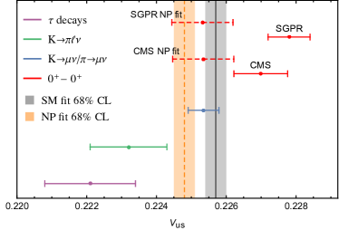
Figure 1: Measurements of $V_{us}$ from $\tau$ decays, $K\to\pi\ell\nu$, ${K\to\mu\nu}/{\pi\to\mu\nu}$, and $0^{+}-0^{+}$ transition using CKM unitarity to convert $V_{ud}$ to $V_{us}$. The grey band shows the 68% C.L. posterior within the SM while the orange band corresponds to the NP fit with nonzero values of $\varepsilon_{ii}$. Here SGPR (CMS) stands for the $V_{us}$ values extracted from super-allowed beta decays using the theory input of Ref. Seng et al. (2018) (Ref. Czarnecki et al. (2019)). Accidentally, the posterior of $V_{us}$ is the same, independently of the theory input used for beta decays (to the numerical accuracy at which we are working).

It is, therefore, very interesting to explore if new physics (NP) can explain this “Cabibbo-angle anomaly.” First of all, note that the absolute size of a NP effect potentially capable of explaining this anomaly is quite large since the corresponding SM contribution is generated at tree-level and is at most suppressed by one power of the Wolfenstein parameter. Because of this, at the level of effective operators, and given the strong LHC bounds on NP generating two-quark-two-lepton operators Aaboud et al. (2017), NP entering via four-fermion operators seems to be a disfavoured option. Another possibility is a modification of $W$-fermion couplings, where a right-handed $W$-coupling to quarks only improves the fit mildly Grossman et al. (2020). Furthermore, a modification of left-handed $W$-couplings to quarks (which is equivalent to an apparent violation of CKM unitarity) can improve the agreement between super-allowed beta decay and $V_{us}$ from kaon decays Belfatto et al. (2020), but generates potentially dangerous effects in other flavour observables (like kaon mixing). Therefore, we will follow a different and novel avenue in this Letter and study the impact of modified (flavour dependent) $W$-boson couplings to neutrinos.

Modified couplings of neutrinos to the SM $W$ are generated via higher dimensional operators in an EFT approach. Here, due to $SU(2)_{L}$ gauge invariance, in general not only $W$-neutrino couplings but also $Z$-neutrino couplings are modified. Moreover, these modified couplings not only enter $Z$ and $W$ decays, but also all low energy observables involving neutrinos. In particular, ratios testing lepton flavour universality (LFU) in $K$, $\pi$ and $W$ decays are most relevant due to their exquisite experimental and theoretical precision. There are stringent bounds from $K\to\mu\nu/K\to e\nu$ Ambrosino et al. (2009); Lazzeroni et al. (2013), $\pi\to\mu\nu/\pi\to e\nu$ Aguilar-Arevalo et al. (2015); Tanabashi et al. (2018) as well as from $\tau\to\mu\nu\nu/\tau\to e\nu\nu$ or $W\to\mu\nu/W\to e\nu$ Alcaraz et al. (2006). Correlated effects arise, and it is clear that a global fit to all data is necessary in order to assess consistently the impact of modified neutrino couplings.

Modified neutrino couplings to SM gauge bosons have already been considered in the literature in the context of right-handed neutrinos Lee and Shrock (1977); Shrock (1980); Schechter and Valle (1980); Shrock (1981a, b); Langacker and London (1988); Bilenky and Giunti (1993); Nardi et al. (1994); Tommasini et al. (1995); Bergmann and Kagan (1999); Loinaz et al. (2003a, b, 2004); Antusch et al. (2006, 2009); Biggio (2008); Alonso et al. (2013); Abada et al. (2013); Akhmedov et al. (2013); Basso et al. (2014); Abada et al. (2014); Antusch and Fischer (2014, 2015); Abada et al. (2016); Abada and Toma (2016a, b); Bolton et al. (2020) and global fits have also been performed Fernandez-Martinez et al. (2016); Chrzaszcz et al. (2020). However, extensions with right-handed neutrinos lead necessarily to destructive interference with the SM, whereas here we will also be interested in the most general case allowing for an arbitrary phase of the NP contribution. The connection to, and correlations with, the Cabibbo-angle anomaly were not considered before and, in addition, we will use the publicly available HEPfit software De Blas et al. (2020) to perform a Bayesian analysis, while previous analyses were based on frequentist inference.

After defining our setup and reviewing the relevant observables together with the corresponding NP modification in the following section II, we will present the results of our fit in the analysis section before we conclude in the final section.

II Setup and observables

As outlined in the introduction, we want to assess the impact of modified neutrino couplings to gauge bosons within an EFT approach. For this purpose, we assume that the NP scale is above the EW scale, as suggested by LHC Butler (2017); Masetti (2018) and LEP Antonelli and Moretti (2002) searches. Therefore, NP interactions must be $SU(2)_{L}$ gauge invariant and the number of operators is significantly reduced Buchmuller and Wyler (1986). In fact, at the dimension 6 level, there is just one operator which modifies only the couplings of gauge bosons to neutrinos Buchmuller and Wyler (1986); Grzadkowski et al. (2010), ${\bar{L}_{i}}{\gamma^{\mu}}\tau^{I}{L_{j}}{H^{\dagger}}i{\mathord{\buildrel{\lower 3.0pt\hbox{$\scriptscriptstyle\leftrightarrow$}}\over{D}}_{\mu}^{I}}H$, with ${\tau^{I}}=\left({1,-{\sigma_{1}},-{\sigma_{2}},-{\sigma_{3}}}\right)$, where $\sigma_{i}$ are the Pauli matrices (i.e., it is the difference of the two operators $Q_{\varphi\ell}^{(1)}$ and $Q_{\varphi\ell}^{(3)}$ in the basis of Ref. Grzadkowski et al. (2010), to which we refer the interested reader for details on the conventions). Note that this operator is Hermitian, meaning the diagonal elements are real. In what follows, we conveniently parametrize the effect of a nonzero Wilson coefficient of this operator in such a way that a neutrino entering a gauge coupling carries a (small) modification of $\frac{1}{2}\varepsilon_{ij}$, resulting in shifts in the $W$ and $Z$ Feynman rules,

$$\frac{{-i{g_{2}}}}{{\sqrt{2}}}{{\bar{\ell}}_{i}}{\gamma^{\mu}}{P_{L}}{\nu_{j}}{W_{\mu}} \Rightarrow\frac{{-i{g_{2}}}}{{\sqrt{2}}}{{\bar{\ell}}_{i}}{\gamma^{\mu}}{P_{L}}{\nu_{j}}{W_{\mu}}\left({{\delta_{ij}}+\frac{1}{2}{\varepsilon_{ij}}}\right)\,,$$

$$\frac{{-i{g_{2}}}}{2c_{W}}{{\bar{\nu}}_{i}}{\gamma^{\mu}}{P_{L}}{\nu_{j}}{Z_{\mu}} \Rightarrow\frac{{-i{g_{2}}}}{2c_{W}}{{\bar{\nu}}_{i}}{\gamma^{\mu}}{P_{L}}{\nu_{j}}{Z_{\mu}}\left({{\delta_{ij}}+{\varepsilon_{ij}}}\right)\,.$$ (1)

Here we assumed massless neutrinos and thus suppressed the PMNS matrix in the $W$ vertex.

Let us then, in the following subsections, consider the observables which will be included in our global fit.

II.1 Lepton flavour violating decays

Non-diagonal elements of $\varepsilon_{ij}$ lead to charged lepton flavour violation. Here the bounds from radiative lepton decays $\ell_{i}\to\ell_{f}\gamma$ are most stringent. Using the results of Ref. Crivellin et al. (2018) we obtain

$$\text{Br}\left(\ell_{i}\rightarrow\ell_{f}\gamma\right)=\frac{m_{\ell_{i}}^{3}}{4\pi\Gamma_{\ell_{i}}}\left|\frac{10e}{384\pi^{2}M_{W}^{2}}\frac{g_{2}^{2}}{2}m_{\ell_{i}}\varepsilon_{fi}\right|^{2}\,,$$ (2)

where we keep only linear terms in $\varepsilon_{if}$ and neglect the small mass of the outgoing lepton. The current experimental 90% C.L. limits on lepton flavour violation processes are $4.2\times 10^{-13}$ and $4.4(3.3)\times 10^{-8}$ for $\mu\rightarrow e\gamma$ Baldini et al. (2016) and $\tau\rightarrow\mu(e)\gamma$ Aubert et al. (2010), respectively, leading to $|\varepsilon_{e\mu}|\leq 1.4\times 10^{-5}$ and $|\varepsilon_{\mu\tau}|\leq 9.4\times 10^{-3}$ and $|\varepsilon_{e\tau}|\leq 1.1\times 10^{-2}$. These limits on the flavour off-diagonal elements can be used directly, as they are unaffected (at leading order in $\varepsilon_{ij}$) by other entries $\varepsilon_{ij}$. Furthermore, since flavour off-diagonal elements of $\varepsilon_{ij}$ in flavour conserving processes do not interfere with the SM contributions, they enter only quadratically. Therefore, $\varepsilon_{ij}$ with $i\neq j$ can be safely neglected in the following observables.

II.2 EW observables

While the measurements of the mass of the $Z$ boson ($m_{Z}$) and the fine structure constant ($\alpha$) are not affected by the modification of the neutrino couplings in Eq. (1), the Fermi constant ($G_{F}$, which is determined with a very high precision from the muon lifetime) is. As such, its value, extracted from $\mu\to e\nu\nu$, depends on the modification of the $W$-$\ell$-$\nu$ coupling. Taking into account that Br($\mu^{+}\rightarrow\mathrm{e}^{+}\nu_{e}\bar{\nu}_{\mu})\sim 1$ we have

$$\frac{1}{\tau_{\mu}}=\frac{(G_{F}^{\mathcal{L}})^{2}m_{\mu}^{5}}{192\pi^{3}}(1+\Delta q)\left(1+\frac{1}{2}\varepsilon_{ee}+\frac{1}{2}\varepsilon_{\mu\mu}\right)^{2}\,,$$ (3)

where $G_{F}^{\mathcal{L}}$ is the Fermi constant appearing in the Lagrangian and $\Delta q$ includes phase space, QED and hadronic radiative corrections. Thus we find

$$\begin{split}G_{F}&=G_{F}^{\mathcal{L}}\left(1+\frac{1}{2}\varepsilon_{ee}+\frac{1}{2}\varepsilon_{\mu\mu}\right)\,.\end{split}$$ (4)

In addition to $G_{F}$, only the total width of the $Z$ ($\Gamma_{Z}$) and the number of light neutrino extracted from invisible $Z$ decays ($N_{\nu}$) receive direct modifications in the presence of anomalous neutrino couplings. The number of active neutrinos, as extracted from data Schael et al. (2006), is given by

$$\begin{split}\text{N}_{\nu}^{\text{exp}}&=(1+\varepsilon_{ee})^{2}+(1+\varepsilon_{\mu\mu})^{2}+(1+\varepsilon_{\tau\tau})^{2}\\ &=2.9840\pm 0.0082\,,\end{split}$$ (5)

which in turn also changes $\Gamma_{Z}$, to which it contributes.

We included the modifications of these observables into the EW implementations of HEPfit De Blas et al. (2020); see the Supplemental Material SM , which includes Refs. Schael et al. (2013); Webber et al. (2011); Aaboud et al. (2018); Sirunyan et al. (2020); Group and Aaltonen (2016); Aaboud et al. (2019); Sirunyan et al. (2019); Cirigliano and Rosell (2007); Czapek et al. (1993); Britton et al. (1992); Bryman et al. (1983); Antonelli et al. (2010); Cirigliano et al. (2012); Awramik et al. (2004); Sirlin (1980); Faisst et al. (2003); Avdeev et al. (1994); Chetyrkin et al. (1995a, b); Broncano et al. (2003); Abada et al. (2007), for further details.

II.3 Test of LFU

In case the diagonal elements of $\varepsilon_{ii}$ differ from each other, observables testing LFU provide stringent constraints. Here, we have ratios of $W$ decays ($W\to\ell_{i}\nu/W\to\ell_{j}\nu$) as well as of kaon, pion and tau decays (see Ref. Pich (2014) for an overview). Concerning $B$ decays, only $B\to D^{(*)}e\nu/B\to D^{(*)}\mu\nu$ provides a relevant constraint Jung and Straub (2019). The corresponding observables, including their dependence on $\varepsilon_{ii}$ are shown in Table 1 of the Supplemental Material SM . For tau decays, we include their correlations as given in Ref. Amhis et al. (2019).

II.4 Determination of $\mathbf{|V_{us}|}$

We can now turn to the determination of $V_{us}$ as already briefly depicted in the introduction (see Fig. 1).

$K_{\ell 3}$: $V_{us}$ can be determined from the semi-leptonic kaon decays. In order to allow for LFU violation, one has to separate muon from electron modes. Averaging $K_{L}$, $K^{\pm}$ and $K_{S}$ modes Tanabashi et al. (2018), one finds

$$\begin{split}|V_{us}^{K_{\mu 3}}|&\simeq 0.2234(8)\,,\qquad|V_{us}^{K_{e3}}|\simeq 0.2230(21)\,,\end{split}$$ (6)

by using the lattice average Aoki et al. (2020) of the form factor at zero momentum transfer $f_{+}(0)=0.9698(17)$, $(N_{f}=2+1+1)$. We choose to include the muon mode in the global fit, while the electron mode is already taken into account via the LFU ratios in Table 1 of the Supplemental Material SM . The NP modification, including the indirect effect of $G_{F}$, is

$$|V_{us}^{K_{\mu 3}}|\simeq|V^{\mathcal{L}}_{us}|\left(1-\frac{1}{2}\varepsilon_{ee}\right)\,.$$ (7)

$K_{\ell 2}$: $\text{Br}(K^{\pm}\rightarrow\mu^{\pm}\nu)/\text{Br}(\pi^{\pm}\rightarrow\mu^{\pm}\nu)$ determines $V_{us}/V_{ud}$. Including long-distance electromagnetic and strong isospin breaking corrections Cirigliano and Neufeld (2011) and using the average of the lattice determinations for the ratio of form factors Aoki et al. (2020) ${f_{K^{\pm}}}/{f_{\pi^{\pm}}}=1.1967(18)$, with $(N_{f}=2+1+1)$, we find

$$|V_{us}^{K/\pi}|\simeq 0.22535(44)\,,$$ (8)

where we assumed CKM unitarity and took $|V_{ub}|\simeq 0.004$. Note that the value of $V_{us}$ is very insensitive to $V_{ub}$, whose uncertainty can therefore be neglected, and that this $V_{ub}$ determination is not affected by $\varepsilon_{ij}$.

$0^{+}-0^{+}$ transitions: $|V_{ud}|$ can be extracted from super-allowed nuclear $\beta$ transitions Hardy and Towner (2016). The result relies heavily on the evaluation of radiative corrections. We consider the two different results (as suggested in Ref. Grossman et al. (2020)) of Marciano et al. Czarnecki et al. (2019) (CMS) and Seng et al. Seng et al. (2019) (SGPR), which produce

$$\begin{split}&|V_{us}|_{\text{CMS}}=0.22699(77)\,,\qquad|V_{us}|_{\text{SGPR}}=0.22780(60)\,,\end{split}$$

where CKM unitarity was again used. Turning on the NP couplings, we find the following modification

$$|V_{us}^{\beta}|\simeq\sqrt{1-|V^{\mathcal{L}}_{ud}|^{2}\left(1-\frac{1}{2}\varepsilon_{\mu\mu}\right)^{2}}.$$ (9)

$\tau$ decays: $|V_{us}|$ can be also determined from hadronic $\tau$ decays Amhis et al. (2019). Here the average is Amhis et al. (2019) $|V_{us}^{\tau}|=0.2221(13)$. Both $\tau\to K\nu/\tau\to\pi\nu$ and the inclusive mode measure $V_{us}/V_{ud}$, which means there is, at leading order, no dependence on $\varepsilon_{ij}$, and the determination is then unaffected by our NP contributions. This is different for the determination from $\tau\to K\nu$, whose dependence on $\varepsilon_{ij}$ is given by

$$|V_{us}^{\tau\to K\nu}|\simeq|V_{us}^{\mathcal{L}}|\left(1-\frac{1}{2}\varepsilon_{ee}-\frac{1}{2}\varepsilon_{\mu\mu}+\frac{1}{2}\varepsilon_{\tau\tau}\right).$$ (10)

Since this mode as well as other hadronic tau decays are already included in the LFU ratios, we do not include the $V_{us}$ from tau decays in our global fit. Nevertheless, we can still predict the change in $V_{us}^{\tau\to K\nu}$.

III Analysis

In this section we perform the global fit to the modified neutrino couplings [see Eq. (1)], taking into account the observables discussed in the previous section. Before presenting the results, let us briefly discuss the statistical inference procedure we adopted. Our analysis is performed in a Bayesian framework using the publicly available HEPfit package De Blas et al. (2020), whose Markov Chain Monte Carlo (MCMC) determination of posteriors is powered by the Bayesian Analysis Toolkit (BAT) Caldwell et al. (2009).

In order not to overweight the $V_{ud}$ measurements from $0^{+}-0^{+}$ transitions, we do not include both theory determinations at the same time, but rather define two scenarios: NP-I with $|V_{ud}|_{\text{CMS}}$ from Ref. Czarnecki et al. (2019), and NP-II with $|V_{ud}|_{\text{SGPR}}$ from Ref. Seng et al. (2018). Bayesian model comparison between different scenarios can be accomplished by evaluating an information criterion (IC) Ando (2007, 2011). This quantity is characterized by the mean and the variance of the posterior of the log-likelihood, $\log\mathcal{L}$, which yield an estimate of the predictive accuracy of the model Gelman et al. (2013), and a penalty factor for the number of free parameters fitted. Preference for a model is given according to the smallest IC value, following the scale of evidence suggested in Refs. Jeffreys (1998); Kass and Raftery (1995). The full list of fit parameters and details on the choice of priors can be found in Supplemental Material SM .

Let us now probe the impact of nonzero values of $\varepsilon_{ij}$. As noted in the last section, one can neglect the flavour off-diagonal elements whose values are directly bounded by radiative lepton decays. As such, in the global fit we only have to consider $\varepsilon_{ee}$, $\varepsilon_{\mu\mu}$, and $\varepsilon_{\tau\tau}$. The 68% C.L. intervals for fit parameters of the flavour sector ($V_{us}^{\mathcal{L}}$, $\varepsilon_{ii}$) within the two NP scenarios can be found in Table 3 of the Supplemental Material SM . One can see that there is only a mild difference between both scenarios. In particular, the posterior of $V_{us}^{\mathcal{L}}$ is accidentally even the same and only the preferred region for $\varepsilon_{ee}$ ($\varepsilon_{\mu\mu}$) in scenario NP-II is slightly more negative (positive) than in scenario NP-I. Therefore, we only present the results for the two dimensional $\varepsilon_{ii}$-$\varepsilon_{jj}$ planes in Fig. 2 within scenario NP-II (scenario NP-I is approximately $1\,\sigma$ more compatible with the SM hypothesis). There, the $68\%$, $95\%$ ad $99\%$ C.L. contours are shown, and it is clear from the $\varepsilon_{ee}$-$\varepsilon_{\mu\mu}$ plane, where the largest deviation from SM can be found, that these regions do not overlap with the SM point $\varepsilon_{ii}=0$, and that $\varepsilon_{ee}$ and $\varepsilon_{\mu\mu}$ possess an anti-correlation.

Concerning the $V_{us}$ determination, we have also depicted the posterior of scenario NP-II and the updated values extracted from super-allowed beta decay in Fig. 1. In summary, the main drivers leading to a better fit of the NP scenarios are the $V_{us}$ determination from super-allowed beta decays, $\tau\to\mu\nu\nu/\mu\to e\nu\nu$ and $\tau\to\mu\nu\nu/\tau\to e\nu\nu$ SM .

For a more direct model comparison between the NP fits and the SM we look at the IC values. Here we obtain for the SM $\text{IC}_{\rm SM}=73$, compared to $\text{IC}_{\rm NP-II}=63$ and $\text{IC}_{\rm NP-I}=60$ for the two NP scenarios. In the vein of Ref. Kass and Raftery (1995), this constitutes “very strong” evidence against the SM, further evidencing that current data clearly favours the NP hypothesis, and promoting the search for a NP model.

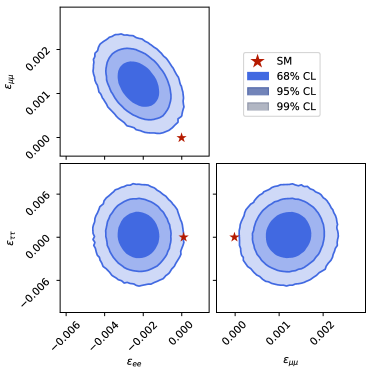
Figure 2: Global fit for scenario NP-II. The 2D fit ($68\%$, $95\%$ and $99\%$ C.L.) for $\varepsilon_{ii}$-$\varepsilon_{jj}$ as well as the 1D fit for each $\varepsilon_{ii}$ ($68\%$ C.L. indication) are shown.

For that UV complete NP explanation obviously the possibility of right-handed neutrinos comes to mind, as these models give tree-level effects in $Z$-$\nu$-$\nu$ and $W$-$\ell$-$\nu$ couplings. However, here the effect is necessarily destructive (i.e., $\varepsilon_{ii}<0$), which is not in agreement with the preferred regions found in our fit. Nonetheless, performing the fit we find: $\varepsilon_{ee}=-0.0013^{+0.0006}_{-0.0006}$, $\varepsilon_{\tau\tau}=-0.0014^{+0.0010}_{-0.0015}$, and $0>\varepsilon_{\mu\mu}>-0.0002$ at $68\%$ C.L. The shift towards values compatible with zero (within $\sim 2.2\,\sigma$ for $\varepsilon_{ee}$, and $1.2\,\sigma$ for $\varepsilon_{\tau\tau}$) signals a feeble improvement with respect to the SM. In fact, such a conclusion is supported by an IC value of 78, which is even bigger than the one of the SM due to the penalty for extra parameters. Moreover, once the constraint from $\mu\to e\gamma$, arising in models with $\varepsilon_{e\mu}=\sqrt{\varepsilon_{ee}\varepsilon_{\mu\mu}}$ Mohapatra and Valle (1986); Bernabeu et al. (1987); Branco et al. (1989); Buchmuller and Wyler (1990); Pilaftsis (1992); Dev and Pilaftsis (2012); Malinsky et al. (2005); Antusch and Fischer (2014); Coy and Frigerio (2019) is taken into account, it is even more difficult in this scenario to explain data well.

Since right-handed neutrinos cannot fully explain the tensions within the EW fit, naturally the quest for a different UV completion arises. Even though a complete analysis is beyond the scope of this work, note that this can be achieved, e.g., by adding additional vectorlike leptons (VLLs) which induce tree-level modifications to $Z$ and $W$ couplings with leptons after EW symmetry breaking. Here, $SU(2)$ singlets and triplets generate the desired Wilson coefficients $C^{(1,3)}_{\phi\ell}$, while $SU(2)$ doublets modify couplings of right-handed charged leptons to $Z$. One has, therefore, four VLLs at our disposal: two doublets and two singlets which differ in hypercharge and contribute as

$$\text{N}\!:\; C_{\phi\ell}^{(3)fi}=-C_{\phi\ell}^{(1)fi}<0,\;\;\text{E}\!:\;C_{\phi\ell}^{(3)fi}=C_{\phi\ell}^{(1)fi}<0,$$

$$\Sigma_{0}\!:\; C_{\phi\ell}^{(3)fi}=\frac{1}{3}C_{\phi\ell}^{(1)fi}>0,\;\;\Sigma_{1}\!:\;C_{\phi\ell}^{(3)fi}=-\frac{1}{3}C_{\phi\ell}^{(1)fi}>0,$$

using the conventions of Ref. de Blas et al. (2018). It is thus clear that we can produce any combination of $C^{(1,3)}_{\phi\ell}$ with arbitrary sign, including $C^{(1)}_{\phi\ell}=-C^{(3)}_{\phi\ell}$ being positive or negative. Such a linear combination of vectorlike leptons might seem ad hoc at first glance. However, this is exactly what happens in composite or extradimensional models with custodial protection Agashe et al. (2003, 2006) [see e.g. Refs. del Aguila et al. (2010); Carmona and Goertz (2013) for a generalization to the lepton sector with $SU(2)_{L}$ triplets]. In such models, the symmetry group is chosen in such a way that the VLL representations (generated for instance as Kaluza-Klein excitations) lead to modifications of $Z$-$\nu$-$\nu$ and $W$-$\ell$-$\nu$ couplings, but not to $Z$-$\ell$-$\ell$ interactions. As this corresponds exactly to the case at hand, $C^{(1)}_{\phi\ell}=-C^{(3)}_{\phi\ell}$, extradimensional or composite models with custodial protection can therefore very well give rise to the scenario obtained in our model-independent fit.

IV Conclusions and Outlook

In this Letter, we performed a model-independent global fit to modified neutrino couplings motivated by the Cabbibo-angle anomaly (i.e., the disagreement between the different determinations of $V_{us}$). Taking into account all relevant observables related to the EW sector of the SM and observables testing LFU (like $\tau\to\mu\nu\nu/\tau\to e\nu\nu$, $\pi\to\mu\nu\nu/\pi\to e\nu\nu$, etc.), we found that agreement with data can be significantly improved by small modifications $\varepsilon_{ii}$. Our results for this NP scenario are depicted in Fig. 2, showing the SM hypothesis lies beyond the 99.99% C.L. region, corresponding to a deviation of more than $4\,\sigma$. Furthermore, the IC values of the scenarios here considered strongly prefer the NP hypothesis.

However, conventional models with right-handed neutrinos, which lead to necessary destructive interference, cannot explain data very well. Nevertheless, since these models are well motivated by the observed nonvanishing neutrino masses, we updated their global fit, taking into account the different $V_{us}$ determinations.

Clearly, more data and further theory input is needed to clarify the situation in the future. Also, the study and construction of NP models which can give a constructive effect in $Z$-$\nu$-$\nu$ and $W$-$\ell$-$\nu$ couplings, in particular strongly coupled theories with custodial protection, is a promising direction of research, building upon the results of this article. Furthermore, as our explanation involves flavour-dependent couplings, the Cabibbo-angle anomaly fits into the bigger picture of deviations from LFU as observed in $b\to s\ell^{+}\ell^{-}$ transitions Capdevila et al. (2018); Altmannshofer et al. (2017); D’Amico et al. (2017); Ciuchini et al. (2017); Hiller and Nisandzic (2017); Geng et al. (2017); Hurth et al. (2017); Algueró et al. (2019); Aebischer et al. (2020); Ciuchini et al. (2019); Arbey et al. (2019) and the anomalous magnetic moment of the muon and electron Davoudiasl and Marciano (2018); Crivellin et al. (2018). This opens up the possibility of so far undiscovered correlations among these observables with UV complete models.

Acknowledgements — We thank Marco Fedele, Julian Heeck, Martin Hoferichter, Ayan Paul, Hugo M. Proença and Mauro Valli for useful discussions and/or help with HEPfit. The work of A.C. is supported by a Professorship Grant (PP00P2_176884) of the Swiss National Science Foundation. A.M.C. acknowledges support by the Swiss National Science Foundation under contract 200021_178967.

Supplemental Material

.1 Electroweak observables

Observable	Ref.	Measurement
$\frac{K\rightarrow\mu\nu}{K\rightarrow e\nu}\simeq|1+\frac{1}{2}\varepsilon_{\mu\mu}-\frac{1}{2}\varepsilon_{ee}|$	Pich (2014)	$0.9978\pm 0.0020$
$\frac{\pi\rightarrow\mu\nu}{\pi\rightarrow e\nu}\simeq|1+\frac{1}{2}\varepsilon_{\mu\mu}-\frac{1}{2}\varepsilon_{ee}|$	Aguilar-Arevalo et al. (2015); Tanabashi et al. (2018)	$1.0010\pm 0.0009$
$\frac{\tau\rightarrow\mu\nu\bar{\nu}}{\tau\rightarrow e\nu\bar{\nu}}\simeq|1+\frac{1}{2}\varepsilon_{\mu\mu}-\frac{1}{2}\varepsilon_{ee}|$	Amhis et al. (2019); Tanabashi et al. (2018)	$1.0018\pm 0.0014$
$\frac{K\rightarrow\pi\mu\bar{\nu}}{K\rightarrow\pi e\bar{\nu}}\simeq|1+\frac{1}{2}\varepsilon_{\mu\mu}-\frac{1}{2}\varepsilon_{ee}|$	Pich (2014)	$1.0010\pm 0.0025$
$\frac{W\rightarrow\mu\bar{\nu}}{W\rightarrow e\bar{\nu}}\simeq|1+\frac{1}{2}\varepsilon_{\mu\mu}-\frac{1}{2}\varepsilon_{ee}|$	Pich (2014); Schael et al. (2013)	$0.996\pm 0.010$
$\frac{\tau\rightarrow e\nu\bar{\nu}}{\mu\rightarrow e\bar{\nu}\nu}\simeq|1+\frac{1}{2}\varepsilon_{\tau\tau}-\frac{1}{2}\varepsilon_{\mu\mu}|$	Amhis et al. (2019); Tanabashi et al. (2018)	$1.0010\pm 0.0014$
$\frac{\tau\rightarrow\pi\nu}{\pi\rightarrow\mu\bar{\nu}}\simeq|1+\frac{1}{2}\varepsilon_{\tau\tau}-\frac{1}{2}\varepsilon_{\mu\mu}|$	Amhis et al. (2019)	$0.9961\pm 0.0027$
$\frac{\tau\rightarrow K\nu}{K\rightarrow\mu\bar{\nu}}\simeq|1+\frac{1}{2}\varepsilon_{\tau\tau}-\frac{1}{2}\varepsilon_{\mu\mu}|$	Amhis et al. (2019)	$0.9860\pm 0.0070$
$\frac{W\rightarrow\tau\bar{\nu}}{W\rightarrow\mu\bar{\nu}}\simeq|1+\frac{1}{2}\varepsilon_{\tau\tau}-\frac{1}{2}\varepsilon_{\mu\mu}|$	Pich (2014); Schael et al. (2013)	$1.034\pm 0.013$
$\frac{\tau\rightarrow\mu\nu\bar{\nu}}{\mu\rightarrow e\nu\bar{\nu}}\simeq|1+\frac{1}{2}\varepsilon_{\tau\tau}-\frac{1}{2}\varepsilon_{ee}|$	Amhis et al. (2019); Tanabashi et al. (2018)	$1.0029\pm 0.0014$
$\frac{W\rightarrow\tau\bar{\nu}}{W\rightarrow e\bar{\nu}}\simeq|1+\frac{1}{2}\varepsilon_{\tau\tau}-\frac{1}{2}\varepsilon_{ee}|$	Pich (2014); Schael et al. (2013)	$1.031\pm 0.013$
$\frac{B\rightarrow D^{(*)}\mu\nu}{B\rightarrow D^{(*)}e\nu}\simeq|1+\frac{1}{2}\varepsilon_{\mu\mu}-\frac{1}{2}\varepsilon_{ee}|$	Jung and Straub (2019)	$0.989\pm 0.012$

Table 1: Ratios testing LFU together with their dependence on the modifications of the neutrino couplings $\varepsilon_{ij}$. Here it is implicitly understood that these ratios are normalized to their values within the SM, such that any deviation from unity measures LFU violation.

Measurements of the EW observables, as performed at LEP Schael et al. (2013, 2006), are high precision tests of the SM. The EW sector of the SM can be completely parametrized by the three Lagrangian parameters $v$, $g_{1}$ and $g_{2}$; then, other quantities like $G_{F}$, $m_{W}$ or $m_{Z}$ can be expressed in terms of these parameters and their measurements allow for consistency tests. However, for practical purposes it is better to choose another set of three parameters parametrizing the EW sector of the SM: a convenient choice is to use the quantities with the smallest experimental error of their direct measurements, i.e. the mass of the $Z$ boson ($m_{Z}$), the Fermi constant ($G_{F}$) and the fine structure constant ($\alpha$).

The EW observables, computed from $G_{F}$, $m_{Z}$ and $\alpha$, are given at the beginning of Table 4. Since the $Z$ sector remains lepton flavour universal (for charged leptons) we can thus use the standard $Z$-pole observables (assuming LFU) Schael et al. (2006). The Higgs mass ($m_{h}$), the top mass ($m_{t}$) and the strong coupling constant ($\alpha_{s}$) have to be included as fit parameters as well, since they enter indirectly EW observables via loop effects.

We point out that in our analysis it is convenient that we use $G_{F}$, not $G_{F}^{\mathcal{L}}$, as a fit parameter whose prior is determined by its direct measurement $1.1663787(6)\times 10^{-5}\,\text{GeV}^{-2}$ Webber et al. (2011). Note that $G_{F}^{\mathcal{L}}$ enters all other EW observables which are thus indirectly modified by $\varepsilon_{ee}$ and $\varepsilon_{\mu\mu}$.

Parameter		Prior		SM posterior
$G_{F}\,\,[{\rm GeV}^{-2}]$ Tanabashi et al. (2018)		$1.1663787(6)\times 10^{-5}$		$\star$
$\alpha$ Tanabashi et al. (2018)		$7.2973525664(17)\times 10^{-3}$		$\star$
$\Delta\alpha_{\rm had}$ Tanabashi et al. (2018)		$276.1(11)\times 10^{-4}$		$275.4(10)\times 10^{-4}$
$\alpha_{s}(M_{Z})$ Tanabashi et al. (2018)		$0.1181(11)$		$\star$
$m_{Z}\,\,[{\rm GeV}]$ Schael et al. (2006)		$91.1875\pm 0.0021$		$91.1883\pm 0.0020$
$m_{H}\,\,[{\rm GeV}]$ Aaboud et al. (2018); Sirunyan et al. (2020)		$125.16\pm 0.13$		$\star$
$m_{t}\,\,[{\rm GeV}]$ Group and Aaltonen (2016); Aaboud et al. (2019); Sirunyan et al. (2019)		$172.80\pm 0.40$		$172.96\pm 0.39$

Table 2: Parameters of the EW fit together with their (Gaussian) priors and posteriors. Here, the posteriors that remain equal to the prior (up to the numerical accuracy considered) are abbreviated by a star. Furthermore, once the effect of $\varepsilon_{ij}$ is included, only the posterior of the top (pole) mass changes slightly to $m_{t}\sim 172.83\,$GeV while all other parameters remain the same, showing the EW fit is, to a very good approximation, independent of the flavour parameters.

		Prior		NP-I posterior		NP-II posterior
$V_{us}^{\mathcal{L}}$		$0.225\pm 0.010$		$0.2248\pm 0.0004$		$0.2248\pm 0.0004$
$\varepsilon_{ee}$		$0.00\pm 0.05$		$-0.0018\pm 0.0006$		$-0.0022\pm 0.0007$
$\varepsilon_{\mu\mu}$		$0.00\pm 0.05$		$0.0008\pm 0.0004$		$0.0012\pm 0.0003$
$\varepsilon_{\tau\tau}$		$0.00\pm 0.05$		$-0.0002\pm 0.0020$		$-0.0003\pm 0.0020$

Table 3: Fit parameters of the flavour sector together with their posteriors for the two NP scenarios. One can see that the choice between the two $V_{us}$ determinations has a small effect on $\varepsilon_{ee}$ and $\varepsilon_{\tau\tau}$, while in scenario NP-I a vanishing value of $\varepsilon_{\mu\mu}$ is more compatible with data (within $\sim 2~{}\sigma$). Note that the value for $V_{us}^{\mathcal{L}}$ is accidentally the same (to the numerical accuracy given): the effect of the different $V_{us}$ determinations is compensated by the difference in the preferred regions for $\varepsilon_{ii}$. However, the deviation from the SM posterior, $0.2257(3)$, is indeed sizable.

Observable	Ref.	Measurement	SM Posterior	NP-I posterior	NP-II posterior	Pull I	Pull II
$M_{W}\,[\text{GeV}]$	Tanabashi et al. (2018)	$80.379(12)$	$80.363(4)$	$80.371(6)$	$80.370(6)$	0.67	0.59
$\Gamma_{W}\,[\text{GeV}]$	Tanabashi et al. (2018)	$2.085(42)$	$2.089(1)$	$2.090(1)$	$2.090(1)$	-0.02	-0.02
$\text{BR}(W\to\text{had})$	Tanabashi et al. (2018)	$0.6741(27)$	$0.6749(1)$	$0.6749(2)$	$0.6749(1)$	0	0
$\text{sin}^{2}\theta_{\rm eff}^{\rm lept}(Q^{\rm had}_{\rm FB})$	Tanabashi et al. (2018)	$0.2324(12)$	$0.2316(4)$	$0.2315(1)$	$0.2315(1)$	-0.1	-0.1
$\text{sin}^{2}\theta_{\rm eff(Tev)}^{\rm lept}$	Tanabashi et al. (2018)	$0.23148(33)$	$0.2316(4)$	$0.2315(1)$	$0.2315(1)$	0.17	0.17
$\text{sin}^{2}\theta_{\rm eff(LHC)}^{\rm lept}$	Tanabashi et al. (2018)	$0.23104(49)$	$0.2316(4)$	$0.2315(1)$	$0.2315(1)$	-0.03	-0.03
$P_{\tau}^{\rm pol}$	Schael et al. (2006)	$0.1465(33)$	$0.1461(3)$	$0.1474(8)$	$0.1472(8)$	-0.14	-0.09
$A_{\ell}$	Schael et al. (2006)	$0.1513(21)$	$0.1461(3)$	$0.1474(8)$	$0.1472(8)$	0.72	0.60
$\Gamma_{Z}\,[\text{GeV}]$	Schael et al. (2006)	$2.4952(23)$	$2.4947(6)$	$2.496(1)$	$2.496(1)$	-0.11	-0.11
$\sigma_{h}^{0}\,[\text{nb}]$	Schael et al. (2006)	$41.541(37)$	$41.485(6)$	$41.495(24)$	$41.493(24)$	0.47	0.42
$R^{0}_{\ell}$	Schael et al. (2006)	$20.767(35)$	$20.747(7)$	$20.749(7)$	$20.749(7)$	0.06	0.06
$A_{\rm FB}^{0,\ell}$	Schael et al. (2006)	$0.0171(10)$	$0.0160(7)$	$0.0163(2)$	$0.0163(2)$	0.12	0.12
$R_{b}^{0}$	Schael et al. (2006)	$0.21629(66)$	$0.21582(1)$	$0.21582(1)$	$0.21582(1)$	0	0
$R_{c}^{0}$	Schael et al. (2006)	$0.1721(30)$	$0.17219(2)$	$0.17220(2)$	$0.17220(2)$	0	0
$A_{\rm FB}^{0,b}$	Schael et al. (2006)	$0.0992(16)$	$0.1024(2)$	$0.1033(6)$	$0.1032(6)$	-0.41	-0.36
$A_{\rm FB}^{0,c}$	Schael et al. (2006)	$0.0707(35)$	$0.0731(2)$	$0.0738(4)$	$0.0738(4)$	-0.20	-0.20
$A_{b}$	Schael et al. (2006)	$0.923(20)$	$0.93456(2)$	$0.9347(1)$	$0.9347(1)$	-0.01	-0.01
$A_{c}$	Schael et al. (2006)	$0.670(27)$	$0.6675(1)$	$0.6680(4)$	$0.6680(3)$	0	0
$\frac{K\rightarrow\mu\nu}{K\rightarrow e\nu}$	Lazzeroni et al. (2013); Ambrosino et al. (2009); Cirigliano and Rosell (2007); Pich (2014)	$0.9978\pm 0.0020$	$1$	$1.00137\pm 0.00046$	$1.00173\pm 0.00043$	-0.63	-0.82
$\frac{\pi\rightarrow\mu\nu}{\pi\rightarrow e\nu}$	Czapek et al. (1993); Britton et al. (1992); Bryman et al. (1983); Cirigliano and Rosell (2007); Aguilar-Arevalo et al. (2015); Tanabashi et al. (2018)	$1.0010\pm 0.0009$	$1$	$1.00137\pm 0.00046$	$1.00173\pm 0.00043$	0.75	0.38
$\frac{\tau\rightarrow\mu\nu\bar{\nu}}{\tau\rightarrow e\nu\bar{\nu}}$	Amhis et al. (2019); Tanabashi et al. (2018)	$1.0018\pm 0.0014$	$1$	$1.00137\pm 0.00046$	$1.00173\pm 0.00043$	0.99	1.24
$\frac{K\rightarrow\pi\mu\bar{\nu}}{K\rightarrow\pi e\bar{\nu}}$	Antonelli et al. (2010); Cirigliano et al. (2012); Pich (2014)	$1.0010\pm 0.0025$	$1$	$1.00137\pm 0.00046$	$1.00173\pm 0.00043$	0.25	0.11
$\frac{W\rightarrow\mu\bar{\nu}}{W\rightarrow e\bar{\nu}}$	Pich (2014); Schael et al. (2013)	$0.996\pm 0.010$	$1$	$1.00137\pm 0.00046$	$1.00173\pm 0.00043$	-0.14	-0.17
$\frac{B\rightarrow D^{(*)}\mu\nu}{B\rightarrow D^{(*)}e\nu}$	Jung and Straub (2019)	$0.989\pm 0.012$	$1$	$1.00137\pm 0.00046$	$1.00173\pm 0.00043$	-0.11	-0.14
$\frac{\tau\rightarrow e\nu\bar{\nu}}{\mu\rightarrow e\bar{\nu}\nu}$	Amhis et al. (2019); Tanabashi et al. (2018)	$1.0010\pm 0.0014$	$1$	$0.9997\pm 0.0010$	$0.9995\pm 0.0010$	-0.04	-0.15
$\frac{\tau\rightarrow\pi\nu}{\pi\rightarrow\mu\bar{\nu}}$	Amhis et al. (2019)	$0.9961\pm 0.0027$	$1$	$0.9997\pm 0.0010$	$0.9995\pm 0.0010$	0.20	0.26
$\frac{\tau\rightarrow K\nu}{K\rightarrow\mu\bar{\nu}}$	Amhis et al. (2019)	$0.9860\pm 0.0070$	$1$	$0.9997\pm 0.0010$	$0.9995\pm 0.0010$	0.06	0.09
$\frac{W\rightarrow\tau\bar{\nu}}{W\rightarrow\mu\bar{\nu}}$	Pich (2014); Schael et al. (2013)	$1.034\pm 0.013$	$1$	$0.9997\pm 0.0010$	$0.9995\pm 0.0010$	-0.02	-0.03
$\frac{\tau\rightarrow\mu\nu\bar{\nu}}{\mu\rightarrow e\nu\bar{\nu}}$	Amhis et al. (2019); Tanabashi et al. (2018)	$1.0029\pm 0.0014$	$1$	$1.0011\pm 0.0011$	$1.0013\pm 0.0011$	1.06	1.17
$\frac{W\rightarrow\tau\bar{\nu}}{W\rightarrow e\bar{\nu}}$	Pich (2014); Schael et al. (2013)	$1.031\pm 0.013$	$1$	$1.0011\pm 0.0011$	$1.0013\pm 0.0011$	0.10	0.11
$|V_{us}^{K_{\mu 3}}|$	Tanabashi et al. (2018); Aoki et al. (2020)	$0.2234\pm 0.0008$	$0.2257(3)$	$0.22509\pm 0.00040$	$0.22516\pm 0.00040$	0.81	0.74
$|V_{us}/V_{ud}|^{K/\pi}$	Cirigliano and Neufeld (2011); Aoki et al. (2020)	$0.2313\pm 0.0005$	$0.2317(4)$	$0.23078\pm 0.00044$	$0.23082\pm 0.00044$	-0.16	-0.10
$|V_{us}^{\tau}|_{\text{incl.}}$	Hardy and Towner (2016); Czarnecki et al. (2019)	$0.2195\pm 0.0019$	$0.2257(3)$	$0.22487\pm 0.00041$	$0.22491\pm 0.00041$	0.48	0.45
$|V_{ud}^{\beta}|_{\text{CMS}}$	Hardy and Towner (2016); Czarnecki et al. (2019)	$0.97389\pm 0.00018$	$0.974185(79)$	$0.97400\pm 0.00017$	-	0.56	-
$|V_{ud}^{\beta}|_{\text{SGPR}}$	Hardy and Towner (2016); Seng et al. (2019)	$0.97370\pm 0.00014$	$0.974185(79)$	-	$0.97379\pm 0.00013$	-	2.57

Table 4: Observables included in and predicted by our global fit. Here the SM scenario, as well as the NP-I and NP-II hypotheses are shown. The pulls are defined with respect to the SM in such a way that positive values means better agreement of the NP hypothesis (highlighted in grey). Note that the observables testing LFU are implicitly normalized in such a way that they correspond to unity within the SM.

.2 Fit results

Employing the Metropolis-Hastings algorithm implemented in BAT to sample from the posterior distribution, our MCMC runs involved 6 chains with a total of 2 million events per chain, collected after an equivalent number of pre-run iterations.

The fit parameters of the EW sector, $G_{F},\,\alpha,\,\alpha_{s},\,M_{Z},\,m_{t}$ and $m_{H}$, are reported in Table 2. Here we assume Gaussian priors, which correspond to the current direct measurements or evaluations of these parameters. We verified that the chosen ranges of flat priors yield well-determined probability density functions (p.d.f.), i.e. they are chosen in such a way that larger ranges would not significantly alter our results.

Concerning the $W$ mass computation, HEPfit provides both the option of using the recent precise numerical formula from Ref. Awramik et al. (2004), and the usual determination of $M_{W}$ from the $Z$-boson mass, $\alpha$, and $G_{F}$ Sirlin (1980), with radiative corrections encoded in $\Delta r$ (which has been known up to 3 loop $\mathcal{O}(\alpha^{3})$ EW Faisst et al. (2003) and $\mathcal{O}(\alpha\alpha_{s}^{2},\,\alpha^{2}\alpha_{s})$ EW-QCD contributions Faisst et al. (2003); Avdeev et al. (1994); Chetyrkin et al. (1995a, b)). Due to the direct modifications of $G_{F}$ under analysis, we opted for the latter.

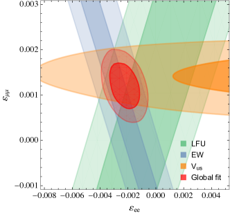
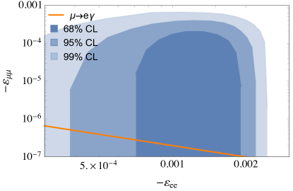
Figure 3: Left: Contributions to the global fit from different classes of observables: LFU (green), EW (blue) and $V_{us}$ (orange). The global fit (red) is superimposed. Dark and light colors correspond to the 68% CL and 95% CL, respectively. Right: Global fit for scenario NP-II confining $\varepsilon_{ii}$ to be negative, as obtained in models with effective PMNS unitarity violation from mixing with right-handed neutrinos Broncano et al. (2003); Abada et al. (2007); Antusch et al. (2006); Antusch and Fischer (2014)and considered in previous fits Fernandez-Martinez et al. (2016); Chrzaszcz et al. (2020). In addition, we show the 90%CL region from $\mu\to e\gamma$ as obtained in simple models with approximate symmetry protecting neutrino masses $\varepsilon_{e\mu}=\sqrt{\varepsilon_{ee}\varepsilon_{\mu\mu}}$ Mohapatra and Valle (1986); Bernabeu et al. (1987); Branco et al. (1989); Buchmuller and Wyler (1990); Pilaftsis (1992); Dev and Pilaftsis (2012); Malinsky et al. (2005); Antusch and Fischer (2014); Coy and Frigerio (2019)

First, we redo the global EW fit within the SM; then, we probe the impact of non-zero values of $\varepsilon_{ij}$. The results of these fits can be found in Tables 2, 3 and 4. Note that the posteriors of EW fit parameters remain practically unchanged once NP effects via $\varepsilon_{ij}$ are included. It worth of mention that this is the case for $G_{F}$ (due to its precise measurement) which is used as a fit parameter, yet not for $G_{F}^{\mathcal{L}}$ whose posterior accidentally assumes (to the precision we are working at) the same value, $(1.16755\pm 0.00089)\times 10^{-5}$, within scenario NP-I and NP-II.

This is, however, not the case for $V_{us}$ where the SM value of $0.2257(3)$ significantly changes once NP is included. Note that the main tensions within the SM originate from $Z\to\nu\nu$, $g_{V}^{\ell}$, and the conflicting determinations of $V_{us}$ from $K_{L}\to\pi\mu\nu$ and super-allowed beta decays. These are also the observables where the most significant improvements (compared to the SM scenario) are achieved in the NP case while the tension in $W\to\tau\nu/W\to e\nu$ cannot be resolved in our NP scenario.

The fit in the $\varepsilon_{ee}$-$\varepsilon_{\mu\mu}$ plane is depicted in the left plot of Fig. 3 where, in addition, the preferred regions from the individual classes of processes are shown. The fact that all regions overlap at the $68\%$ CL reflects the goodness of the fit.

In order to better judge the agreement of the NP hypotheses with data and how this compares to the SM, we define the pull (with respect to the SM) for an observable $O_{i}$ as

$$P(O_{i})=\left|\frac{O_{i}^{\text{exp}}-O_{i}^{\text{SM}}}{\sqrt{(\sigma_{i}^{\text{exp}})^{2}+(\sigma_{i}^{\text{SM}})^{2}}}\right|-\left|\frac{O_{i}^{\text{exp}}-O_{i}^{\text{NP}}}{\sqrt{(\sigma_{i}^{\text{exp}})^{2}+(\sigma_{i}^{\text{NP}})^{2}}}\right|\,.$$ (11)

These pulls are reported in Table 4 for the two NP scenarios, where also the SM and NP posteriors for all observables (except the EW fit parameters shown in Fig. 2 which are unaffected by the NP parameters) are shown. Pulls signalling a better agreement between NP and data (with respect to the SM) are highlighted in gray.

Finally, we show in the right plot of Fig. 3 the constraints in the $\varepsilon_{ee}\varepsilon_{\mu\mu}$ plane for the case in which the modified gauge boson couplings to leptons are generated by a right-handed neutrino.

References

- de Blas et al. (2016) J. de Blas, M. Ciuchini, E. Franco, S. Mishima, M. Pierini, L. Reina, and L. Silvestrini, JHEP 12, 135 (2016), arXiv:1608.01509 [hep-ph] .
- Haller et al. (2018) J. Haller, A. Hoecker, R. Kogler, K. Mönig, T. Peiffer, and J. Stelzer, Eur. Phys. J. C78, 675 (2018), arXiv:1803.01853 [hep-ph] .
- Aaltonen et al. (2018) T. A. Aaltonen et al. (CDF, D0), Phys. Rev. D97, 112007 (2018), arXiv:1801.06283 [hep-ex] .
- Ciuchini et al. (2001) M. Ciuchini, G. D’Agostini, E. Franco, V. Lubicz, G. Martinelli, F. Parodi, P. Roudeau, and A. Stocchi, JHEP 07, 013 (2001), arXiv:hep-ph/0012308 [hep-ph] .
- Hocker et al. (2001) A. Hocker, H. Lacker, S. Laplace, and F. Le Diberder, Eur. Phys. J. C21, 225 (2001), arXiv:hep-ph/0104062 [hep-ph] .
- Cabibbo (1963) N. Cabibbo, Phys. Rev. Lett. 10, 531 (1963).
- Kobayashi and Maskawa (1973) M. Kobayashi and T. Maskawa, Prog. Theor. Phys. 49, 652 (1973).
- Butler (2017) J. N. Butler (CMS), in 5th Large Hadron Collider Physics Conference (LHCP 2017) Shanghai, China, May 15-20, 2017 (2017) arXiv:1709.03006 [hep-ex] .
- Masetti (2018) L. Masetti (ATLAS), Proceedings, 7th Workshop on Theory, Phenomenology and Experiments in Flavour Physics: The Future of BSM Physics (FPCapri 2018): Anacapri, Capri, Italy, June 8-10, 2018, Nucl. Part. Phys. Proc. 303-305, 43 (2018).
- Lusiani (2019) A. Lusiani, Proceedings, 15th International Workshop on Tau Lepton Physics (TAU2018): Amsterdam, Netherlands, September 24-28, 2018, SciPost Phys. Proc. 1, 001 (2019), arXiv:1811.06470 [hep-ex] .
- Amhis et al. (2019) Y. S. Amhis et al. (HFLAV), (2019), arXiv:1909.12524 [hep-ex] .
- Aoki et al. (2020) S. Aoki et al. (Flavour Lattice Averaging Group), Eur. Phys. J. C 80, 113 (2020), arXiv:1902.08191 [hep-lat] .
- Seng et al. (2018) C.-Y. Seng, M. Gorchtein, H. H. Patel, and M. J. Ramsey-Musolf, Phys. Rev. Lett. 121, 241804 (2018), arXiv:1807.10197 [hep-ph] .
- Seng et al. (2019) C. Y. Seng, M. Gorchtein, and M. J. Ramsey-Musolf, Phys. Rev. D100, 013001 (2019), arXiv:1812.03352 [nucl-th] .
- Gorchtein (2019) M. Gorchtein, Phys. Rev. Lett. 123, 042503 (2019), arXiv:1812.04229 [nucl-th] .
- Czarnecki et al. (2019) A. Czarnecki, W. J. Marciano, and A. Sirlin, Phys. Rev. D100, 073008 (2019), arXiv:1907.06737 [hep-ph] .
- Grossman et al. (2020) Y. Grossman, E. Passemar, and S. Schacht, JHEP 07, 068 (2020), arXiv:1911.07821 [hep-ph] .
- Aaboud et al. (2017) M. Aaboud et al. (ATLAS), JHEP 10, 182 (2017), arXiv:1707.02424 [hep-ex] .
- Belfatto et al. (2020) B. Belfatto, R. Beradze, and Z. Berezhiani, Eur. Phys. J. C 80, 149 (2020), arXiv:1906.02714 [hep-ph] .
- Ambrosino et al. (2009) F. Ambrosino et al. (KLOE), Eur. Phys. J. C64, 627 (2009), [Erratum: Eur. Phys. J.65,703(2010)], arXiv:0907.3594 [hep-ex] .
- Lazzeroni et al. (2013) C. Lazzeroni et al. (NA62), Phys. Lett. B719, 326 (2013), arXiv:1212.4012 [hep-ex] .