Survival of Primordial Planetary Atmospheres: Mass Loss from Temperate Terrestrial Planets
Abstract
The most widely-studied mechanism of mass loss from extrasolar planets is photoevaporation via XUV ionization, primarily in the context of highly irradiated planets. However, the EUV dissociation of hydrogen molecules can also theoretically drive atmospheric evaporation on low-mass planets. For temperate planets such as the early Earth, impact erosion is expected to dominate in the traditional planetesimal accretion model, but it would be greatly reduced in pebble accretion scenarios, allowing other mass loss processes to be major contributors. We apply the same prescription for photoionization to this photodissociation mechanism and compare it to an analysis of other possible sources of mass loss in pebble accretion scenarios. We find that there is not a clear path to evaporating the primordial atmosphere accreted by an early Earth analog in a pebble accretion scenario. Impact erosion could remove 2,300 bars of hydrogen if 1% of the planet’s mass is accreted as planetesimals, while the combined photoevaporation processes could evaporate 750 bars of hydrogen. Photodissociation is likely a subdominant, but significant component of mass loss. Similar results apply to super-Earths and mini-Neptunes. This mechanism could also preferentially remove hydrogen from a planet’s primordial atmosphere, thereby leaving a larger abundance of primordial water compared to standard dry formation models. We discuss the implications of these results for models of rocky planet formation including Earth’s formation and the possible application of this analysis to mass loss from observed exoplanets.
1 Introduction
Conventional planet formation models assume the build-up of isolation mass cores from the growth of solids into planetesimals (e.g., Safronov & Zvjagina 1969; Wetherill & Stewart 1993; Goldreich et al. 2004; Benz et al. 2014). In the classical picture, isolation mass oligarchs (with masses comparable to Mars and semimajor axes AU) are built up through collisions of planetesimals aided by gravitational focusing. They collide violently in the chaotic growth phase after dissipative gas is largely gone at system ages 10 – 100 Myr. These planets may form without any primordial atmospheres if the isolation mass is reached after the gas disk dissipates. If they do accrete atmospheres, however, their subsequent thermal evolution and mass loss are almost certainly dominated by giant impacts (Biersteker & Schlichting, 2019). Building up an Earth-mass planet through successive giant impacts would likely have removed any primordial volatiles, and any thin, primordial atmosphere surviving these impacts could be quickly lost to photoevaporation (Johnstone et al., 2019).
An important alternative theory of planet formation involves the streaming instability and pebble accretion, which can form terrestrial planets faster than planetesimal accretion, i.e., while the circumstellar disk is still gas rich (e.g., Bitsch et al. 2015; Chambers 2018). In a pebble-accretion scenario, a super-Earth-mass planet could form within 1 Myr and capture a much deeper gas-rich envelope. Estimates from Ginzburg et al. (2016) suggest that mass fractions up to 2% could be realized in a hydrogen- and helium-rich atmosphere. If the nebula is “wet” (e.g., Ciesla & Cuzzi 2006) due to the migration of small icy bodies interior to the ice-line (and subsequent sublimation of volatiles into the gas phase), an Earth-mass planet could capture a water mass fraction approaching , comparable to the present-day Earth within a factor of 3 (Meech & Castillo-Rogez, 2015).
It is not clear that the above results are consistent with formation models explaining the inner solar system planets, as discussed below. Nonetheless, it is of interest whether there are mechanisms that could deplete light elements in the primordial atmosphere. In this paper, we explore processes that could contribute to mass loss over the lifetime of such a planet. Most notably, we explore the possibility that molecular photodissociation by ultraviolet light could be an important source of mass loss. This mechanism has not been explored thoroughly in the context of mass loss from young exoplanets. This process should be effective, however, because photodissociation of hydrogen occurs at lower energies than photoionization (Draine & Bertoldi, 1996; Heays et al., 2017), and thus would increase the ultraviolet flux available for upper atmosphere heating and escape. Draine & Bertoldi (1996) also estimate the broad-spectrum efficiency of photodissociation at 15%, which would also increase the total mass loss over photoionization alone. In contrast, mass loss on exoplanets is usually modeled based only on photoionization of hydrogen atoms (Watson et al., 1981). For completeness, we also investigate other sources of mass loss and quantify their relative importance.
A related question is whether this mass loss of hydrogen and helium will leave behind any of the water accreted from the disk. It is an interesting coincidence that the expected amount of water accreted from the disk is similar to the mass of Earth’s oceans. This finding may indeed be mere coincidence because for many years, isotopic evidence has indicated that the majority of the water in Earth’s oceans must have originated from beyond the ice line. In particular, the D/H ratio is indicative of cold cloud chemistry, such as that observed in molecular cloud cores (and presumably delivered to the outer nebula during the early phases of star formation). On the other hand, measurements of D/H ratios in deep mantle lava are closer to the solar ratio, indicating the possibility of a deep mantle reservoir of primordial water (van Dishoeck et al., 2014; Hallis et al., 2015), which could have been accreted from the primordial circumstellar disk. While this possibility remains speculative, exploring mass loss processes that could leave primordial water behind could shed light on whether these findings are consistent with pebble accretion formation models.
The pebble accretion scenario has additional complications. Notably, pebble accretion has a natural endpoint at a super-Earth mass (e.g. Bitsch et al. 2015; Johansen & Lambrechts 2017). In order to produce an Earth-mass planet, the accumulation phase must be interrupted by some other mechanism, and this process may also affect the volatile content of the planet. Also, pebble accretion cannot be the only process involved in the formation of our solar system’s terrestrial planets because any theory of planet formation must still explain the Moon-forming impact and Mercury’s iron-rich composition (e.g. Ward & Canup 2000; Benz et al. 2007). Nonetheless, we can place reasonable limits on the extent of these other processes, and we find that they may be comparable to photoevaporation for planets with relatively low insolation like early Earth, but they probably do not dominate mass loss in most cases.
This paper is structured as follows. In Section 2, we summarize the current literature on mass loss from exoplanets, particularly to justify our addition of photodissociation to the list of viable processes. In Section 3, we compute the anticipated mass loss from several mechanisms, including both photoionization and photodissociation, along with a summary of the published results for impact erosion and their potential application to a pebble accretion scenario. In Section 4, we apply these results to observable properties of exoplanets and discuss their implications for formation models of planets and planetary systems. We summarize our findings in Section 5.
2 Summary of Literature
Most studies of atmospheric loss from extrasolar planets are based directly or indirectly on the work of Watson et al. (1981). This work considered energy-limited mass loss due to heating by extreme ultraviolet (EUV) radiation from the star. This mechanism is dominant for planets that are highly irradiated, including a large fraction of known exoplanets. Although this paper considers additional mass loss mechanisms such as Jeans escape and thermal winds, we focus primarily on photoevaporation, which continues to dominate even at Earth’s level of insolation when impact erosion is not considered.
Watson et al. (1981) did not define the term “EUV”. Although they describe the limit of efficient EUV heating to take place when the gas is ionized, they describe the heating only in terms of absorption, rather than photoexitation. EUV radiation is conventionally taken to be the radiation blueward of either 121 nm or 91.2 nm, meaning that this convention does not necessarily faithfully model the ionizing flux, which is strictly blueward of 91.2 nm. Dissociation of molecular hydrogen occurs primarily via line processes blueward of 111 nm (Draine & Bertoldi, 1996), so dissociating radiation may or may not be included in the definition of “EUV” depending on the context.
In addition, most studies of atmospheric loss from exoplanets use directly or indirectly the estimates of Ribas et al. (2005) for the XUV flux as a function of time for solar-analog stars. This model integrated the X-ray and UV flux over the wavelength range 0.1 – 120 nm, again not modeling the exact ionizing flux. This previous work also did not include stars of other spectral types. However, some studies used different models of XUV flux, e.g. Murray-Clay et al. 2009; Lammer et al. 2014. Meanwhile, photodissociation has been addressed for exoplanets in other contexts such as water loss (Jura, 2004), but very little in the context of hydrogen-rich atmosphere loss.
While Watson et al. (1981) dealt specifically with Earth and Venus, the majority of scholarship on atmospheric loss from exoplanets has focused on hot jupiters (e.g., Lammer et al. 2003; Baraffe et al. 2004; Hubbard et al. 2007). (Here, we are taking “hot jupiters” generically to be planets with equilibrium temperatures 1,000 K and mass greater than Saturn, MJ.) Nonetheless, studies of mass loss from hot jupiters often do not clearly specify whether photoionization or photodissociation processes are considered.
Murray-Clay et al. (2009) modeled mass loss on hot jupiters incorporating a number of non-thermal processes. They did consider dissociation, but they only considered thermal dissociation, not photodissociation, and they concluded that the temperatures involved were high enough for the hydrogen to be fully thermally dissociated. For their specific model of energy-limited ultraviolet heating, they explicitly considered only photoionization, and as such included only UV radiation blueward of 91.2 nm.
Lopez et al. (2012) and their subsequent papers studied mass loss from super-Earths and mini-Neptunes. However, they also cited the Ribas et al. (2005) model for XUV flux, and they explicitly described it as modeling only ionization, not dissociation. Following from this model, Jin et al. (2014) described the problem in the same manner while recreating the models of Baraffe et al. (2004) and Lopez et al. (2012). Meanwhile, Howe & Burrows (2015) did mention both ionization and dissociation as possible pathways of XUV heating, but they also used the Ribas et al. (2005).
Finally, Lammer et al. (2014) considered both ionization and dissociation processes. (They also made some mention of “FUV” fluxes, although they did not define the term.) However, their mass loss model was based only on XUV fluxes and thus also did not take photodissociation into account in practice.
The above discussion thus indicates that photodissociation-induced atmospheric evaporation has received little attention in applications to exoplanets. Nonetheless, the energy levels involved indicate that this process should be taken into account when modeling exoplanet evolution. In this case, to leading order, the same model for mass loss applies, except that the wavelength range modeled should be set to cover the full range of dissociating radiation in addition to ionizing radiation, and the efficiency factor should be adjusted accordingly.
3 Estimates of Mass Loss
For this analysis of mass loss, we consider pebble accretion taking place within the ice line (Chambers, 2016) of a circumstellar disk. This scenario results in the rapid formation of a planet, which is assumed to have the same mass and orbital distance as Earth. As an initial condition, the planet captures an additional 2% of its mass from the gas disk before dissipation (Ginzburg et al., 2016). The resulting 0.02 atmosphere corresponds to a surface pressure of 23,000 bar, which we use to quantify the mass loss from the various processes. (For comparison, one ocean in the form of water vapor would be 230 bar.) Such an atmosphere will be optically thick, keeping the surface hot with an estimated surface temperature of 4,500 K (Popovas et al., 2018), and with a Kelvin-Helmholtz cooling time of 3 Myr (Miller-Ricci et al., 2009). These parameters represent our starting conditions for purely thermodynamic loss processes such as Jeans escape and thermal winds.
At this temperature, the atmosphere is likely to be inflated to a radius . As an order of magnitude estimate, the scale height of a hydrogen atmosphere will be 200 km, and the height of the atmosphere will be 30-40 scale heights from the surface to the exobase, resulting in a total height of . The actual height of the atmosphere must be determined by a numerical calculation, which is beyond the scope of this paper (but cf. Howe et al. (2014) at high entropy levels). As a result, we assume an initial exosphere radius of km in our model. For comparison, planetesimal accretion models predict the planet to be repeatedly heated to a temperature 1,500 K (about 6-9 times) by giant impacts during its formation phase, thereby resulting in a thinner atmosphere and a shorter cooling time.
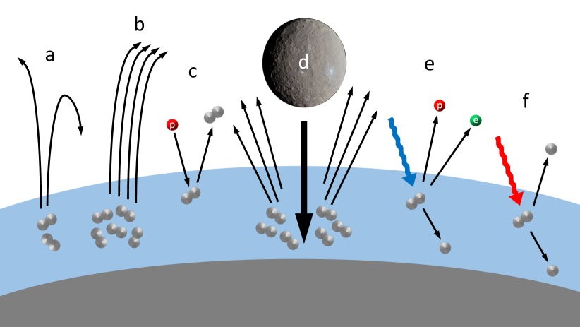
A number of different processes can contribute to atmospheric mass loss, although not all authors agree on the nomenclature (e.g. Catling & Zahnle 2009; Catling & Kasting 2017). Here, we group the relevant mass loss mechanisms into two broad categories, including (i) thermal escape and (ii) atmospheric erosion. The first class of mechanisms occurs when the atmosphere is heated, causing the constituent molecules to escape into space. Thermal escape can be considered in the limit where individual molecules escape from a collisionless exosphere (Jeans escape, Section 3.1), or when the outflow takes place in the fluid limit and is driven by atmospheric heating (hydrodynamic escape, Section 3.2). In this latter case, different heating mechanisms come into play, where this paper considers approximate treatments of both ionization heating (Section 3.5) and dissociation heating (Section 3.6). The second class of mechanisms, atmospheric erosion, includes ablation by stellar winds (Section 3.3) and impact erosion, which takes place as large bodies impinge upon the atmosphere (Section 3.4).111For completeness, we note that supra-thermal escape can also occur. In this setting, individual particles are accelerated to escape velocity due to chemical reactions or ionic interactions. These mechanisms are generally subdominant and are not considered here (Catling & Kasting, 2017). These mass loss mechanisms are depicted schematically in Figure 1.
3.1 Jeans Escape
The first means of atmospheric mass-loss is Jeans escape. In this case, the atoms and/or molecules in the high-velocity tail of the Maxwell-Boltzmann distribution are moving fast enough to escape the gravity well of the planet (Catling & Zahnle, 2009). The particles in this high-energy tail continually escape from the top of the atmosphere. Jeans escape is considered significant if the escape velocity is less than about six times the mean molecular speed, which occurs on Earth only for hydrogen and helium.
Jeans escape depends on the temperature of the exosphere and is thus exponentially increased when the young planet is heated by rapid accretion. The rate of Jeans escape (in molecules per unit area per unit time) can be derived from the Maxwell-Boltzmann distribution and is given by
| (1) |
where is the most probable molecular speed, and is the escape parameter, given by . The density of the exobase, , is determined by setting the scale height equal to the mean free path, i.e.,
| (2) | |||
| (3) |
where is the cross section of the molecules, and is the mean molecular weight. At a temperature of = 4,500 K, the hydrogen gas will be dissociated (which will not be the case at later times when photoexcitation becomes more important), so we must use the values for atomic hydrogen with a molecular weight of u and an atomic diameter of picometers.
Because of the low density of molecules at the exobase, Jeans escape is slow, and relatively little mass can be removed from the thick atmosphere in our model. Even at very high temperatures, the rate of escape increase only slowly with temperature, scaling with , so this conclusion would remain valid even if our temperature estimate is too low. In this model, if we assume km, then the mass loss rate of hydrogen from the planet is g/s. For a time span of 3 Myr, the total mass loss would be about . In terms of pressure, this result implies that Jeans escape is sufficient to evaporate 0.6 bars of hydrogen from an Earth-like primordial atmosphere.
3.2 General Hydrodynamic Escape
In the limit where the gas is coupled (the fluid limit), hydrodynamic winds provide an important description of mass loss. These winds can remove mass from the upper atmosphere at a rate determined by the temperature of the atmosphere. We can estimate the outflow rate for the case of an isothermal atmosphere, which is expected to be a good approximation to a planet’s upper atmosphere, based on the requirement that the flow must pass smoothly through the sonic point222Whereas this section presents the general mechanism for hydrodynamical escape, later sections consider specific heating mechanisms, but utilize an approximate description of the dynamics (Sections 3.5, 3.6). Other forces can further suppress hydrodynamic escape such as magnetic fields (Owen & Adams, 2014), but these are beyond the scope of this paper. The full derivation of these results is given in Appendix A. In the isothermal approximation, the thermal wind from the atmosphere is given by
| (4) |
where is the density at the base of the outflow, , is the sound speed, and the parameter is a function of the dimensionless potential . To first order, this parameterization can be approximated with the expressions
| (5) | ||||
| (6) |
To evaluate the mass loss rate from Equation (4), we need to determine the number density at the base of the flow. For example, when the mass loss is driven by incoming UV photons, the base occurs where the incoming radiation becomes optically thick and the expression for mass loss becomes
| (7) |
where the values use to compute this are specified in the Appendix. (Note that this assumes .)
Because the parameter depends on the sound speed, it is temperature-dependent. Specifically, . For typical exospheric properties of and K predicted by planetesimal accretion models, km s-1, and . If we define the prefactor , then for , . takes on a maximum value of 0.81 for . At higher temperatures, the flow does not transition smoothly through the sonic point and will be time-dependent, or will take on the form of a shock, while at low temperatures, it is exponentially suppressed.
In this paper, we consider two major regimes of hydrodynamic escape. First, there is the short-lived, large-radius, high-temperature state caused by heating due to pebble accretion or giant impacts. For conditions of = 3,000 K and , approaches its maximum value of 0.8, which yields a mass loss over 3 Myr of , corresponding to 118 bars of hydrogen removed from an Earth-like primordial atmosphere.
Second, we consider a quasi-steady state outflow due to ultraviolet heating over the lifetime of the planet. This regime is extremely temperature-sensitive, but if we assume optimistic values for this regime of = 1,500 K and , then , then the integrated mass loss over 5 Gyr is 0.026 , which is greater than the initial hydrogen content of our model and justifies using the energy-limited approximation for computing mass loss up to the order of this quantity.
3.3 Ablation by Stellar Winds
Stellar winds can erode planetary atmospheres by directly imparting momentum to the upper atmosphere through the action of wind particles. This effect can be calculated from the mass loss rate and speed of the stellar wind. The mass loss rate from young stars as a function of time can be described with a simple model of the form (Skumanich & Eddy, 1981),
| (8) |
where the benchmark mass loss rate for Sun-like stars is yr-1, and the time scale = 100 Myr (Wood et al., 2002). We can find an upper limit to the planetary mass loss driven (directly) by the stellar wind by first finding the total amount of (stellar) mass that flows through the volume subtended by the planet, i.e.,
| (9) |
where is the radius of the planet, and is the radius of the planetary orbit (assumed here to be circular). The total mass that intercepts the planet is thus about g. Notice that we are assuming R⊕ instead of the exospheric radius because we are considering the problem over a longer time scale of 100 Myr, over which time the planet would cool, and the atmosphere would compress so that the effective radius will be near that of the solid surface.
The amount of mass that can be directly removed by the incoming wind is limited by conservation of momentum: . Since the wind speed is about km/s, and the escape speed from the planet is about km s-1, the incoming mass could (at most) remove a mass of . Stellar wind ablation can remove only 10 bars of hydrogen from an Earth-like primordial atmosphere, much less than any other processes under consideration.
3.4 Impact Erosion
While giant impacts are generally a feature of planetesimal formation models, it is clear that they will occur regardless of the formation mechanism. In particular, the mass loss caused by giant impacts in the context of the Moon-forming collision has been studied for some time, with a range of results. For example, Ahrens (1993), implied that the Moon-forming impact could have unbound Earth’s entire atmosphere by itself, whereas Genda & Abe (2003) estimated only a 20% atmosphere loss. However, the general theory of mass loss caused by possible multiple giant impacts of a range of sizes is more complex.
Giant impacts can cause mass loss from planets in two ways: [1] The direct mechanical ejection of a large fraction of the atmosphere, and [2] Through the thermal wind induced by the heating of the remaining atmosphere. Both of these mechanisms can be major contributors to mass loss, with magnitudes comparable to or greater than the other mechanisms under consideration.
The mechanical ejection of the atmosphere by impacts over a wide range of impactor sizes was studied by Schlichting et al. (2015). They identified four regimes based on the size of the impactor and additional energy considerations. For small impactors, the shock generated by the impact (or airburst) is not strong enough to eject any of the atmosphere. Slightly larger impacts may be approximated such that they can remove all of the atmosphere up to a certain airmass, thus ejecting a cone above the impact point. The threshold for this ejection is approximated such that the mass of solid ejecta () is greater than the atmosphere mass per unit solid angle. As such, the minimum impactor size for mass ejection varies with the thickness of the atmosphere. For an Earth-like atmosphere, quite small impacts can reach this threshold, but for a primordial atmosphere with a mass of 0.02 , this minimum size is km.
As the impactor size grows, the ejected cone widens until it reaches the horizon, thus ejecting the entire spherical cap above the tangent plane to the impact. For our primordial atmosphere model, this critical impactor size is km. In the third regime, from this size scale up to km, the amount of mass loss is constant as a function of impactor size, and is still determined by the spherical cap above the tangent plane. Finally, for truly giant impactors of km, regardless of atmosphere mass, direct transfer of momentum through the solid mass of the planet will eject significantly more of the atmosphere than the spherical cap (Schlichting et al., 2015).
Planetesimal accretion predicts Mars-sized impactors as a distinct population. Interestingly, these giant impacts are not predicted to eject the entire atmosphere. Indeed, even with equal-mass impactors, tens of percent of their atmospheres would be ejected, but not the entire atmosphere (Schlichting et al., 2015). Ten Mars-sized impactors in sequence, however, could plausibly remove virtually all of the primordial atmosphere from an Earth-mass planet over the course of planet formation. In this case, any remaining atmosphere would have to be produced via outgassing.
Another surprising result of Schlichting et al. (2015) is that while total mass lost will be dominated by giant impacts, smaller bodies produce the most efficient atmosphere stripping in terms of mass of gas ejected per unit mass of impactor. The optimal case occurs for small impactors near the minimum size for ejection, which have an ejection efficiency of 20%. This extremal case provides an upper bound for impact erosion that can be also be applied to pebble accretion: no more than 20% of the mass accreted in the form of planetesimals (with km in our example) will be ejected from the atmosphere.
The other important process in impact erosion is the thermal wind induced by the heating of the atmosphere after the impact (Biersteker & Schlichting, 2019). This heating would also inflate the atmosphere, not just by several Earth radii, but potentially all the way to the Bondi radius at tens of Earth radii (or the Hill radius for close-in planets, for which it is smaller). Such an extended atmosphere will thermally evaporate much more quickly than any of the processes we study in this work. However, the amount of mass lost via thermal wind following a giant impact depends on the base temperature of the atmosphere, for which models indicate a wide range of possibilities. Biersteker & Schlichting (2019) modeled scenarios with base temperatures ranging from 2,000 K, for which the mass loss is negligible, to 10,000 K, for which almost the entire envelope is evaporated in 2 Myr (with a comparable cooling timescale). While these numbers are approximate, for the most likely temperatures it appears that mechanical ejection is dominant over thermal winds.
Unfortunately, the left-over mass from pebble accretion that would form into planetesimals is not well-studied, and its quantity is uncertain. Planetesimal accretion models often postulate a “late veneer” scenario (e.g. Schlichting et al. 2012), in which Earth accreted an additional 1% of its mass from small bodies after the final assembly of the planets. However, this is not necessarily a good guide for the pebble accretion scenario we consider because models that invoke pebble accretion can form planets much faster, in less than 1 Myr, and their solid particle dynamics are very different, being influenced by the gas disk, given that typical gas disk lifetimes are 3 Myr for sun-like stars. In this model, we consider only impacts occurring after the dissipation of the gas disk, i.e. after the atmosphere has finished accreting.
Planetesimal accretion and pebble accretion can potentially coexist in comparable amounts during the gas disk lifetime (Schoonenberg et al., 2019), but late-stage planetesimal accretion in a pebble accretion model is expected to be (cf. Madhusudhan et al. 2017 and Fig. 7 of Liu et al. 2019). Thus, we adopt a value of 0.01 of planetesimals accreted within our pebble accretion scenario as a plausible upper bound, with the caveat that the true number could differ by an order of magnitude. If this mass increment in planetesimals is deposited on the planetary surface with an ejection efficiency of 20%, including thermal winds, 0.002 of gas will be lost. In this toy model, impact erosion will remove 2,300 bars of hydrogen from the planet, any Moon-forming impacts notwithstanding.
3.5 XUV Photo-Ionization and Evaporation
The standard prescription for mass loss on super-Earths, due to Watson et al. 1981, is to assume an energy-limited approximation for ionization by XUV photons, using a specific efficiency factor, usually 10%. This is an optimistic approximation for hydrodynamic escape, but it often applies for low stellar fluxes (e.g. Murray-Clay et al. 2009; Owen & Wu 2017), so we likewise use is as an optimistic approximation for our analysis.
To compute the mass loss rate due to photoevaporation, consider that the escape energy per unit mass is given by the gravitational potential, , and the energy intercepted by the planet is . Assuming an efficiency factor , the total mass loss rate is then given by
| (10) |
where is the radius of the planet at the altitude at which XUV photons are absorbed. For a hydrogen atmosphere in Earth gravity, the UV cross section for atomic hydrogen is cm2, and the photosphere occurs at a pressure of nbar. Note that this assumes a certain percentage of the intercepted XUV energy is converted to kinetic energy of lost particles (and consequently encapsulated by the efficiency factor), not just one atom lost per XUV photon. A tidal correction must be applied to planets orbiting very close to their parent stars, but for our model, we assume it to be negligible.
Because we wish to express the mass loss in terms of surface pressure, this expression can be simplified. The mass of the planet cancels out, so that for a cumulative XUV flux, , impinging on the atmosphere, the integrated atmospheric loss is
| (11) | |||||
where “1 bar” represents an atmosphere mass of .
The XUV flux from a Solar-type star is estimated at 1 AU by Ribas et al. (2005) as a function of age in Gyr, :
| (12) | |||
| (13) |
Note that this expression is an overestimate because it covers the wavelength range of 1 – 118 nm rather than the 1 – 91 nm of interest here (although this range will become relevant again in Section 3.6). However, we use this estimate here because it is the standard for modeling mass loss from irradiated exoplanets. For our model, we assume R R⊕ for the purposes of photoevaporation, given the high temperature and low molecular weight of the primordial atmosphere, but cooler and more compact than the more extended atmosphere present immediately after formation.
To compute the total mass loss based on this formula precisely would require modeling the depth and scale height of the atmosphere over time. However, a rough estimate can be made by computing the total XUV radiation absorbed by the planet over its lifetime. For our general results, compute the integrated mass loss over 5 Gyr, which is both the median age of planet host stars in the solar neighborhood (Bonfanti et al., 2016) and is close to the age of our own solar system. While the stellar XUV flux falls off significantly within a few hundred Myr, we integrate all the way to 5 Gyr for completeness. Note, however, that for the particular case of Earth, planet formation models must account for the apparent loss of the primordial atmosphere at much earlier times.
The integrated XUV flux in our model over 5 Gyr is erg cm-2. With an efficiency of 10%, the total mass of hydrogen lost to photoionization from the prescription in Eq. 13 is 750 bars. As a consistency check, in Section 3.6 we obtain a very similar result with a more precise prescription for the ionizing flux.
XUV irradiation from the central star is not the only potential source of ionizing radiation in the planet’s environment. The galactic background of FUV radiation, usually taken to be erg s-1 cm-2 (91 – 200 nm), is negligible. However, most stars are born in clusters. The mean XUV flux in the birth cluster is likely to be a few erg s-1 cm-2, which is subdominant, but fluxes near the center of the birth cluster may be as much as 100 times greater, comparable to the flux from the parent star (Fatuzzo & Adams, 2008). As a result, a planet in a solar system forming in an especially favorable position in the birth cluster may experience up to twice as much photoevaporation as a planet orbiting an isolated star. Note also that these results assume the star’s X-ray flux saturates at an age of 100 Myr, in accordance with the Ribas et al. (2005) model. If it saturates at an earlier time, the star’s initial XUV flux will be higher, allowing for greater mass loss in the first 100 Myr of the planet’s history.
3.6 EUV Photo-Dissociation and Evaporation
We now consider a second mechanism for ultraviolet-induced photoevaporation. In addition to ionization, longer-wavelength photons of 91 – 111 nm (11.2-13.7 eV) are sufficient to photodissociate hydrogen molecules (Draine & Bertoldi, 1996). This dissociation is a second pathway to input energy into the upper atmosphere and drive evaporation, analogous to the action of ionization, and suggests that the usual convention of 10% efficiency of photoevaporation may be underestimated. Both of these wavelength regimes stand in contrast to the case of longer wavelength photons, which mostly undergo elastic scattering and do not input energy.
In addition to considering a second ultraviolet heating process, we can obtain a more precise estimate of the XUV flux from the fit of Ribas et al. (2005). For greater accuracy, they broke down their fit into five wavelength bins, the reddest of which is 92 – 118 nm. Each bin is fit with a function of the form . For this subsection, we compute the flux of the individual wavelength bins for a more precise result, which can also be applied to photoionization. We multiply the reddest bin by 0.73 to include only the flux with enough energy to dissociate hydrogen (91 – 111 nm).
An even more precise model is available from Claire et al. (2012), who fitted the same parameters to International Ultraviolet Explorer spectra of solar analogs. However, they found an integrated flux over the 2 – 118 nm range about 30% lower than the Ribas et al. (2005) model, so to be generous, we use the Ribas et al. (2005) fit.
For completeness, we note that previous authors have used different long wavelength cutoffs for the relevant XUV and EUV bands (cf. Ingersoll 1969; Lee 1984; Wu & Chen 1993).
| (nm) | ||
|---|---|---|
| 0.1-2 | 2.40 | -1.92 |
| 2-10 | 4.45 | -1.27 |
| 10-36 | 13.5 | -1.20 |
| 36-92 | 4.56 | -1.00 |
| 92-111 | 1.85 | -0.85 |
With these fits, we can compute a better estimate of the absorbed XUV and FUV flux over the Sun’s lifetime by integrating over each bin and adding it to our estimate of a pure blackbody. The integrated fluxes over each bin are shown in Table 2. This table also shows the corresponding atmosphere loss to photoevaporation, assuming an efficiency of 10% at all wavelengths.
| (nm) | Flux over 100 Myr (erg cm2) | Flux over 5 Gyr (erg cm2) | Atmosphere Loss (bar) |
|---|---|---|---|
| 0.1-2 | 171 | ||
| 2-10 | 118 | ||
| 10-36 | 330 | ||
| 36-92 | 93 | ||
| 92-111 | 34 | ||
| 0.1-111 | 746 |
With an efficiency factor of 10%, the combined ionizing and dissociating flux impinging on a young, Earth-like planet could remove about 750 bars of hydrogen, or about 0.065% of the mass of our model planet. We compute the losses due to ionizing flux specifically at 712 bars, 5% less than our estimate using a single-component model for the stellar flux.
For completeness, we note that using the energy limited approximation, provides an upper limit to the expected evaporation rates. For sufficiently strong radiation fluxes (usually associated with very short-period planets) and hence large mass loss rates, the efficacy of UV heating tends to saturate (e.g., Murray-Clay et al. 2009; Owen & Adams 2014), so that the linear relationship in equation (10) breaks down (the mass loss rate increases more slowly than a linear function of the radiation flux). Although such considerations are beyond the scope of this paper, future work should consider more sophisticated models of this process that go beyond the energy limited regime.
3.7 Total Mass Loss
The previous subsections have outlined the various mechanisms through which mass loss can take place. Jeans escape (Section 3.1) corresponds to the limiting case where the escaping molecules are collisionless. Because this process takes place high in the atmosphere, where the density is low, this mechanism is inefficient. In the opposite limit where the atmosphere is collisional, the outflowing material behaves as a fluid. The most restrictive case, described in Section 3.2 and denoted here as a “hydrodynamic wind,” explicitly requires the flow to pass smoothly through its sonic transition. This hydrodynamic model applies for different heating mechanisms. We consider the case of heating from both photoionization (Section 3.5) and photodissociation (Section 3.6) for the case where the outflow is energy-limited. We also consider outflow driven by stellar wind ablation (Section 3.3) and impact erosion (Section 3.4), where the latter provides a substantial contribution.
The results of the models indicate that photodissociation is a non-negligible contribution to mass loss on a young, Earth-like planet formed by pebble accretion, and photoevaporation in general is dominant over all other mechanisms other than impact erosion even before accounting for the potential greater efficiency due to the dissociation contribution to upper atmosphere heating. Because the amount of impact erosion in pebble accretion is uncertain, it is possible that photoevaporation could be dominant. Nonetheless, the total mass loss we compute for all of the processes we study for our model planet is 3.1, or 2.7 kbar, only 15% of the mass of the initial hydrogen envelope. The contributions of each of these mechanisms to the total are listed in Table 3.
| Process | Mass Removed (bars) | Mass Removed () |
|---|---|---|
| Jeans Escape | 0.6 | 50 |
| Stellar Wind Ablation | 20 | 8 |
| Impact Erosion11Based 0.01 of impactor mass. | 2,300 | 2,000 |
| Photoionization | 712 | 619 |
| Photodissociation | 34 | 30 |
| Total | 3,067 | 2,700 |
The difficulty, as noted above, is that planet formation models that seek to explain rapid terrestrial planet formation must strip any primary atmosphere early in the planet’s history, and the total mass loss we find for an early Earth analog is not sufficient. It may yet be possible to evaporate the entire primordial atmosphere if the fraction of late planetesimal accretion is greater, closer to 5-10% of Earth’s mass rather than 1%. Otherwise, the initial gas accretion must be significantly less efficient, leading to a less massive initial atmosphere. The prescription for accretion in Ginzburg et al. (2016) suggests that the accreted mass of hydrogen could vary by perhaps a factor of 2. The efficiency of photoevaporation may also be higher, accounting for the overlap between the ionizing and dissociating radiation wavelength ranges, but even an efficiency of 25% would increase the total mass loss by only 50%, far from sufficient to evaporate all of the hydrogen and helium. The most plausible scenario in this context would seem to be pebble accretion followed multiple late giant impacts of the Moon-forming type could potentially strip the entire atmosphere.
4 Discussion and Implications
Given an Earth-like planet formed by pebble accretion that accretes 2% of its mass in hydrogen and helium from the gas disk, we are unable to find a clear path to evaporating all of this atmosphere. However, for the purpose of modeling exoplanets, energy-limited photodissociation could be a significant contributor to photoevaporation and should be incorporated into existing models of mass loss. This has significant implications for the location of the evaporation valley in radius-flux space.
Yet it is also true that there are several mechanisms that could reduce the predicted mass loss. For photoevaporation, a further complication is that its efficiency may be reduced due to energy loss from line cooling. Both Ly cooling and metal line cooling have been considered in the case of photoionization (Murray-Clay et al., 2009). When photodissociation is added, molecular lines must also be included and will further enhance this effect. Of particular concern is that, for water dissociation, some of the photon energy will be lost to rotational and vibrational modes of the hydroxide radical, reducing the mass loss efficiency by over much of the FUV range. However, the relatively low abundance of water in the primordial atmosphere means this is a negligible effect compared with the evaporation of hydrogen. Dissociation of molecular hydrogen does not have this concern because the dissociated atoms have no molecular lines.
Additionally, magnetic fields are predicted to suppress mass loss in hot jupiters (Adams, 2011; Owen & Adams, 2014). If the surface fields are of order 1 gauss, then magnetic fields may be sufficient to suppress outflows from terrestrial planets. This would reduce our expected mass loss for most processes except for impact erosion, but a full treatment of this problem is beyond the scope of this paper.
Our photodissociation model of mass loss may also be applied to close-orbiting exoplanets. Observations indicate that this population appears to have been significantly sculpted by mass loss (Fulton & Petigura, 2018). For these highly irradiated planets, photoevaporation is usually assumed to dominate over impact erosion even in a planetesimal accretion scenario. This work suggests a possible mechanism for even greater mass loss than is usually predicted, and further study is needed to determine whether adding photodissociation to mass loss models improves modeling of the evaporation valley.
5 Summary and Conclusions
This paper has explored a collection of mass loss mechanisms that can sculpt the atmospheres of Earth-like planets during their first few hundred million years of evolution. These calculations are presented in the context of a fast pebble accretion scenario for terrestrial planet formation, where the resulting planets can capture a significant atmosphere before dissipation of the gas disk, but the results are more broadly applicable. We review various mechanisms that could contribute, assess their importance, and discuss their impact on the resulting composition of the atmosphere. In particular, we discuss whether the dominant hydrogen and helium envelopes can be removed, thereby leaving water and other heavy volatile molecules on the planet. Our primary conclusions can be listed as follows:
-
1.
Photodissociation of molecular species can be a significant source of mass loss in the early evolution of temperate planetary atmospheres in addition to photoionization.
-
2.
Impact erosion in a pebble accretion scenario is uncertain, but could easily dominate mass loss on young terrestrial planets. This process can remove 2,000 bars in our model.
-
3.
Other sources of mass loss (including Jeans escape, traditional forms of a thermal wind, and ablation by stellar winds), are unlikely to contribute significantly in the scenario we explore here.
-
4.
Within the context of our model, where the planet forms rapidly in the presence of a gas rich disk, the early Earth is expected to develop an atmosphere of bars. However, there is not a clear path to evaporating the bulk of this primordial hydrogen and helium.
-
5.
The remaining atmosphere would be enriched in water and perhaps other volatiles because of the preferential loss of hydrogen (and helium) in the outer atmosphere.
More work is needed to understand the timescales (and nature) of planet formation in the pebble accretion scenario, investigate impact erosion in a self-consistent way in this context, and further constrain the distribution of volatile elements in the gas rich disk during terrestrial planet formation via rapid pebble accretion inside the ice-line. We further suggest that researchers studying mass loss in temperate planet atmospheres consider the impact of photodissociation in their models. This initial effort has calculated mass loss rates using a (standard) energy limited approximation with a fixed efficiency; future work should generalize this approach, especially to consider efficiency as a function of wavelength given the two processes involved.
References
- Adams (2011) Adams, F. C. 2011, ApJ, 730, 27
- Ahrens (1993) Ahrens, T. J. 1993, Annual Review of Earth and Planetary Sciences, 21, 525
- Baraffe et al. (2004) Baraffe, I., Selsis, F., Chabrier, G., Barman, T. S., Allard, F., Hauschildt, P. H., & Lammer, H. 2004, A&A, 419, L13
- Benz et al. (2007) Benz, W., Anic, A., Horner, J., & Whitby, J. A. 2007, Space Sci. Rev., 132, 189
- Benz et al. (2014) Benz, W., Ida, S., Alibert, Y., Lin, D., & Mordasini, C. 2014, in Protostars and Planets VI, ed. H. Beuther, R. S. Klessen, C. P. Dullemond, & T. Henning, 691
- Biersteker & Schlichting (2019) Biersteker, J. B., & Schlichting, H. E. 2019, MNRAS, 485, 4454
- Bitsch et al. (2015) Bitsch, B., Lambrechts, M., & Johansen, A. 2015, A&A, 582, A112
- Bonfanti et al. (2016) Bonfanti, A., Ortolani, S., & Nascimbeni, V. 2016, A&A, 585, A5
- Catling & Kasting (2017) Catling, D. C., & Kasting, J. F. 2017, Atmospheric Evolution on Inhabited and Lifeless Worlds
- Catling & Zahnle (2009) Catling, D. C., & Zahnle, K. J. 2009, Scientific American, 300, 36
- Chambers (2018) Chambers, J. 2018, ApJ, 865, 30
- Chambers (2016) Chambers, J. E. 2016, ApJ, 825, 63
- Ciesla & Cuzzi (2006) Ciesla, F. J., & Cuzzi, J. N. 2006, Icarus, 181, 178
- Claire et al. (2012) Claire, M. W., Sheets, J., Cohen, M., Ribas, I., Meadows, V. S., & Catling, D. C. 2012, ApJ, 757, 95
- Draine & Bertoldi (1996) Draine, B. T., & Bertoldi, F. 1996, ApJ, 468, 269
- Fatuzzo & Adams (2008) Fatuzzo, M., & Adams, F. C. 2008, ApJ, 675, 1361
- Fulton & Petigura (2018) Fulton, B. J., & Petigura, E. A. 2018, AJ, 156, 264
- Genda & Abe (2003) Genda, H., & Abe, Y. 2003, Icarus, 164, 149
- Ginzburg et al. (2016) Ginzburg, S., Schlichting, H. E., & Sari, R. 2016, ApJ, 825, 29
- Goldreich et al. (2004) Goldreich, P., Lithwick, Y., & Sari, R. 2004, ApJ, 614, 497
- Hallis et al. (2015) Hallis, L. J., Huss, G. R., Nagashima, K., Taylor, G. J., Halldórsson, S. A., Hilton, D. R., Mottl, M. J., & Meech, K. J. 2015, Science, 350, 795
- Heays et al. (2017) Heays, A. N., Bosman, A. D., & van Dishoeck, E. F. 2017, A&A, 602, A105
- Howe & Burrows (2015) Howe, A. R., & Burrows, A. 2015, ApJ, 808, 150
- Howe et al. (2014) Howe, A. R., Burrows, A., & Verne, W. 2014, ApJ, 787, 173
- Hubbard et al. (2007) Hubbard, W. B., Hattori, M. F., Burrows, A., Hubeny, I., & Sudarsky, D. 2007, Icarus, 187, 358
- Ingersoll (1969) Ingersoll, A. P. 1969, Journal of Atmospheric Sciences, 26, 1191
- Jin et al. (2014) Jin, S., Mordasini, C., Parmentier, V., van Boekel, R., Henning, T., & Ji, J. 2014, ApJ, 795, 65
- Johansen & Lambrechts (2017) Johansen, A., & Lambrechts, M. 2017, Annual Review of Earth and Planetary Sciences, 45, 359
- Johnstone et al. (2019) Johnstone, C. P., Khodachenko, M. L., Lüftinger, T., Kislyakova, K. G., Lammer, H., & Güdel, M. 2019, A&A, 624, L10
- Jura (2004) Jura, M. 2004, ApJ, 605, L65
- Lammer et al. (2003) Lammer, H., Selsis, F., Ribas, I., Guinan, E. F., Bauer, S. J., & Weiss, W. W. 2003, ApJ, 598, L121
- Lammer et al. (2014) Lammer, H., et al. 2014, MNRAS, 439, 3225
- Lee (1984) Lee, L. C. 1984, ApJ, 282, 172
- Liu et al. (2019) Liu, B., Ormel, C. W., & Johansen, A. 2019, A&A, 624, A114
- Lopez et al. (2012) Lopez, E. D., Fortney, J. J., & Miller, N. 2012, ApJ, 761, 59
- Madhusudhan et al. (2017) Madhusudhan, N., Bitsch, B., Johansen, A., & Eriksson, L. 2017, MNRAS, 469, 4102
- Meech & Castillo-Rogez (2015) Meech, K. J., & Castillo-Rogez, J. C. 2015, IAU General Assembly, 22, 2257859
- Miller-Ricci et al. (2009) Miller-Ricci, E., Meyer, M. R., Seager, S., & Elkins-Tanton, L. 2009, ApJ, 704, 770
- Murray-Clay et al. (2009) Murray-Clay, R. A., Chiang, E. I., & Murray, N. 2009, ApJ, 693, 23
- Owen & Adams (2014) Owen, J. E., & Adams, F. C. 2014, MNRAS, 444, 3761
- Owen & Wu (2017) Owen, J. E., & Wu, Y. 2017, ApJ, 847, 29
- Popovas et al. (2018) Popovas, A., Nordlund, Å., Ramsey, J. P., & Ormel, C. W. 2018, MNRAS, 479, 5136
- Ribas et al. (2005) Ribas, I., Guinan, E. F., Güdel, M., & Audard, M. 2005, ApJ, 622, 680
- Safronov & Zvjagina (1969) Safronov, V. S., & Zvjagina, E. V. 1969, Icarus, 10, 109
- Schlichting et al. (2015) Schlichting, H. E., Sari, R., & Yalinewich, A. 2015, Icarus, 247, 81
- Schlichting et al. (2012) Schlichting, H. E., Warren, P. H., & Yin, Q.-Z. 2012, ApJ, 752, 8
- Schoonenberg et al. (2019) Schoonenberg, D., Liu, B., Ormel, C. W., & Dorn, C. 2019, arXiv e-prints, arXiv:1906.00669
- Skumanich & Eddy (1981) Skumanich, A., & Eddy, J. A. 1981, in NATO ASIC Proc. 68: Solar Phenomena in Stars and Stellar Systems, ed. R. M. Bonnet & A. K. Dupree, 349–397
- van Dishoeck et al. (2014) van Dishoeck, E. F., Bergin, E. A., Lis, D. C., & Lunine, J. I. 2014, in Protostars and Planets VI, ed. H. Beuther, R. S. Klessen, C. P. Dullemond, & T. Henning, 835
- Ward & Canup (2000) Ward, W. R., & Canup, R. M. 2000, Nature, 403, 741
- Watson et al. (1981) Watson, A. J., Donahue, T. M., & Walker, J. C. G. 1981, Icarus, 48, 150
- Wetherill & Stewart (1993) Wetherill, G. W., & Stewart, G. R. 1993, Icarus, 106, 190
- Wood et al. (2002) Wood, B. E., Müller, H.-R., Zank, G. P., & Linsky, J. L. 2002, ApJ, 574, 412
- Wu & Chen (1993) Wu, C. Y. R., & Chen, F. Z. 1993, J. Geophys. Res., 98, 7415
Appendix A Derivation of Thermal Wind Mass Loss Rate
The rate of thermal wind erosion from a planetary atmosphere can be estimated from a reduced version of the equations of motion where the flow is taken to be isothermal, which is a reasonable approximation for the upper atmosphere. For this case, the solutions for the dimensionless fluid fields can be found analytically, including the required conditions for the flow to pass smoothly through the sonic transition. In order to complete the solution, we must then specify the values for the physical parameters, i.e., the density at the exobase (the inner boundary of the flow) and the sound speed .
A.0.1 Formulation of the Wind/Outflow Problem
The equations of motion for this problem include the continuity equation,
| (A1) |
the force equation,
| (A2) |
and the energy equation
| (A3) |
We consider the gravitational potential to be that of the planet, which is taken to be spherical with mass and radius . Since the planet spins, the full potential has an additional contribution from the rotating frame of reference. The order of this correction term is , which has size near the planet’s surface and can be ignored in this treatment.
In the energy equation (A3), is the specific energy of the fluid, is the heating rate (per unit volume), and is the cooling rate. To start, we consider the gas to be isothermal and replace the energy equation with the simple equation of state
| (A4) |
A.1 Reduced Equations of Motion
In this section, we consider steady-state solutions and spherical symmetry. In this regime, the continuity and force equations thus reduce to the forms
| (A5) |
Next, we assume that the flow is isothermal with constant sound speed and define the following dimensionless quantities,
| (A6) |
Here, is the radius of the planet and is the density at the inner boundary = 1. The continuity equation thus takes the form
| (A7) |
and the force equation becomes
| (A8) |
where
| (A9) |
These equations can be integrated immediately to obtain the solutions
| (A10) |
and
| (A11) |
where the parameters and are constant.
A.2 Sonic Point Conditions
In order for the flow to pass smoothly through the sonic point, only particular values of the constant are allowed. To quantify this constraint, the boundary conditions at the planetary surface take the form
| (A12) |
where the final equality follows from the continuity equation evaluated at the surface. Since is determined by the conditions at the sonic point, is specified. The remaining parameter is determined by evaluating the force equation at the inner boundary of the flow, i.e.,
| (A13) |
The outflow starts with subsonic speeds so that , whereas typical planet properties imply that . As a result, we can use the approximation .
For the equations of motion (A10) and (A11), the required matching conditions at the sonic point take the form
| (A14) |
The value of the parameter that allows for smooth flow through the sonic point is given by
| (A15) |
Equation (A15) provides an implicit solution for the parameter . However, the term on the right hand side of equation (A15) is extremely small (equal to ) and can be ignored to leading order; doing so results in an explicit solution for the parameter , which can be written in the form
| (A16) |
A.3 Estimating the Physical Constants
The previous subsections specify the solutions for the dimensionless fluid fields, including the necessary conditions for passing smoothly through the sonic point and specification of the dimensionless mass outflow rate . In this section, we complete the solution by estimating values for the physical parameters and that determine the full mass outflow rate, where
| (A17) |
We first note that the dimensionless potential can be written
| (A18) |
To estimate the density at the base of the flow, we start by assuming that incoming radiation heats the atmosphere down to a layer where the incoming UV photons are optically thick. If the atmosphere is isothermal with scale height , then the number density has the form
| (A19) |
and the optical depth as a function of height (measured from the planetary surface) takes the form
| (A20) | ||||
where cm-2 is the cross section for hydrogen to absorb the incoming UV radiation. Setting , we thus find the starting estimate for the density
| (A21) |
For a thin atmosphere, the scale height is given by
| (A22) |
The number density at the base of the flow then becomes
| (A23) |
It is thus useful to define a fiducial mass loss rate
| (A24) | ||||
where is the molecular weight for atomic hydrogen (since the dominant heating process we consider is dissociating). Then, taking an optimistic value of km. The full mass loss rate can then be written,
| (A25) |