Dynamical quantum collapse and an experimental test

Abstract

The quantum measurement problem may have a resolution in de Broglie-Bohm theory in which measurements lead to dynamical wavefunction collapse. We study the collapse in a simple setup and find that there may be slight differences between probabilities derived from standard quantum mechanics versus those from de Broglie-Bohm theory in certain situations, possibly paving the way for an experimental test.

The quantum measurement problem has a long history, dating back to the discovery of quantum mechanics, sometimes stated in terms of “wavefunction collapse” or the “projection postulate”. The essence of the problem is that the quantum state is supposed to change instantaneously and in a stochastic, non-Hamiltonian way when a measurement is made. The collapse is even more puzzling because the detector is built from microscopic constituents whose interactions with the quantum system should be described by Hamiltonian evolution.

A variety of ideas have been proposed to resolve the quantum measurement problem (see Bassi et al. (2013) for a review). Here we will adapt the de Broglie-Bohm (dBB) idea as applied specifically to a non-relativistic, spinless, quantum particle (for related references see Bohm (1952a, b); Holland (1993); Struyve (2004); Perez et al. (2006); Valentini (2007); Ryssens (2019); Bassi and Ghirardi (2003); Bassi et al. (2005); Gasbarri et al. (2017); Nikolic (2012)). In this approach, the particle is described by the wavefunction, $\psi(t,x)$, and a classical realization, $r(t)$. The wavefunction evolves according to the Schrodinger equation; the realization evolves according to an equation of motion that we will specify below. The constituents of the detector are quantum but there is a collective coordinate (e.g. center of mass coordinate) that is well described by a classical variable and is the “pointer” variable. The particle is “detected”, by definition, once the wavefunction has collapsed on to the detector. We will describe the system in more detail in Sec. I.

Our strategy in this paper is to consider a quantum particle in a one-dimensional, infinite square well in which we also place a detector that can detect the particle’s position. Initially the particle is in its ground state and the rules of quantum mechanics (QM) tell us that the detection probability is given by the square of the wavefunction. Using the dBB theory we recover this result but by a dynamical process in which we explicitly see the collapse of the wavefunction. Then we study the situation when there are multiple detectors placed within the square well. In this case, the rules of quantum mechanics would still lead to the usual detection probability given by the square of the wavefunction. However wavefunction collapse is a dynamical process in dBB theory and time-evolution in the presence of several detectors differs from that when there is only one detector. Roughly speaking, it takes time for the wavefunction to collapse at the location of a detector and so the probability density $|\psi(t,x)|^{2}$ changes with time and the probability for a given detector to detect the particle is not simply given by the initial probability density $|\psi(0,x)|^{2}$. This result is sensitive to the classical nature of the detector – to the number of microscopic degrees of freedom that are represented in the collective coordinate – and the differences between QM and dBB are most dramatic for small detectors. This leads to the possibility of experimentally distinguishing standard QM from dBB theory, and to a possible resolution of the quantum measurement problem.

I System

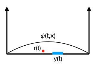
Figure 1: A sketch of the infinite square well with a particle and a single detector (represented by the blue horizontal bar). The variables in the dBB theory are the wavefunction $\psi(t,x)$ of the quantum particle, the particular realization $r(t)$ of the paricle, and the classical variable, $y(t)$, of the detector.

We consider a quantum particle with position variable $x$ and a particle detector in a one-dimensional, infinite square well as sketched in Figure 1. The detector is made up of a number of microscopic degrees of freedom. Call these $\xi_{i}$ where $i=1,\ldots,N$. Then the Hamiltonian can be written as

$$H = \frac{p_{x}^{2}}{2m}+V(x)+\sum_{i}\frac{p_{\xi_{i}}^{2}}{2\mu}+U_{1}(\{|\xi_{i}-\xi_{j}|\})$$ (1)

$$+U_{2}\biggr{(}\sum_{i}\xi_{i}/N\biggr{)}-\lambda W(x)\sum_{i}\xi_{i}$$

Here we use standard notation: $p_{x}$ and $p_{\xi_{i}}$ refer to conjugate momenta for $x$ and $\xi_{i}$; $m$ and $\mu$ are masses of the quantum particle and the detector microscopic degrees of freedom; $V(x)$ is the infinite square well potential

$$V(x)=\begin{cases}0,&x\in[-L,L]\\ \infty,&{\rm otherwise}\end{cases}$$ (2)

$U_{1}(\{|\xi_{i}-\xi_{j}|\})$ is some potential function for the relative internal coordinates of the detector; $U_{2}$ is the potential for the collective coordinate of the detector, taken to be

$$y\equiv\frac{1}{N}\sum_{i}\xi_{i}$$ (3)

The “window function” $W(x)$ defines the range of $x$ in which there is interaction with the detector. For example, this might be a Gaussian function, $W(x)\propto\exp(-x^{2}/2\sigma^{2})$. For simplicity, we will choose the window function to be a top-hat,

$$W(x)=\begin{cases}1&x\in[x_{0}-d,x_{0}+d]\\ 0,&{\rm otherwise}\end{cases}$$ (4)

where $x_{0}$ is the central location of the detector and $2d$ is its full width.

The Hamiltonian can now be written as

$$H = \frac{p_{x}^{2}}{2m}+V(x)$$ (5)

$$+\frac{p_{y}^{2}}{2N\mu}+U_{2}(y)-\lambda NyW(x)+\ldots$$

where the ellipsis denote terms that describe the internal degrees of freedom of the detector and will be ignored.

The detector collective coordinate $y$ is taken to be classical. This is a valid approximation when the wavefunction for $y$ is in the form of a tight wavepacket that remains tight throughout the evolution. For a free particle the time-scale for the spreading of the wavepacket is inversely proportional to the mass of the particle. So our classical treatment of $y(t)$ should be valid for large $N\mu$. Then we may write,

$$H=\frac{p_{x}^{2}}{2m}+V(x)-\lambda NW(x)y(t)+H(y(t))$$ (6)

The Schrodinger equation can now be written as

$$-\frac{1}{2m}\partial_{x}^{2}\psi+V(x)\psi-\lambda Ny(t)W(x)\psi=i\partial_{t}\psi$$ (7)

while the equation for the classical variable $y$ is

$$N\mu{\ddot{y}}+\partial_{y}U_{2}(y)=\lambda NW(x)$$ (8)

The problem is that (8) involves the classical variable $y$ and the quantum variable $x$ through $W(x)$. In the semiclassial approximation $W(x)$ would be replaced by its expectation value. Here however we will replace $x$ by a “realization” of the particle’s position, $r(t)$. This modification – that interactions occur between realizations – is not discussed in dBB theory but seems like a natural extension. So the $y$ equation becomes,

$$N\mu{\ddot{y}}+\partial_{y}U_{2}=\lambda NW(r(t))$$ (9)

We now need an equation for the realization $r(t)$.

The probability distribution $|\psi(t=0,r)|^{2}$ is used to choose the initial value $r(t=0)$. Subsequently $r(t)$ obeys the “guidance equation” of dBB theory Bohm (1952a, b),

$$m{\dot{r}}=\partial_{r}S(t,r)$$ (10)

where $S$ is the phase of the wavefunction: $\psi(t,x)=R(t,x)\exp(iS(t,x))$ where $R$ and $S$ are real. Note that we do not restrict $R$ to be non-negative. The functions $R$ and $S$ will vary smoothly, even through points where $R=0$.

To summarize, the equations describing the quantum particle and the detector are:

$$-\frac{1}{2m}\partial_{x}^{2}\psi+V(x)\psi-\lambda Ny(t)W(x)\psi=i\partial_{t}\psi$$ (11)

$$\mu{\ddot{y}}+\frac{1}{N}\partial_{y}U_{2}(y)=\lambda W(r)$$ (12)

$$m{\dot{r}}=\partial_{r}S(t,r)$$ (13)

where $r(t=0)$ is drawn from the probability distribution $|\psi(t=0,r)|^{2}$. The initial conditions for the detector variable are taken to be $y(0)=0={\dot{y}}(0)$.

We can generalize the model to several detectors by summing over detector variables and window functions. For $D$ identical detectors, the equations become,

$$-\frac{1}{2m}\partial_{x}^{2}\psi+V\psi-\lambda N\sum_{i=1}^{D}y_{i}(t)W_{i}(x)\psi = i\partial_{t}\psi$$ (14)

$$\mu{\ddot{y}}_{i}+\frac{1}{N}\partial_{y_{i}}U_{2}(\{y_{i}\})=\lambda W_{i}(r),$$ (15)

$$m{\dot{r}}=\partial_{r}S(t,r)$$ (16)

The function $U_{2}$ determines the nature of the detector, for example, how will the detector respond if there is no detection? Here we will consider the case that the detector state does not change unless there is an interaction with the particle realization and, for simplicity, set $U_{2}=0$. Then the state of the detector changes only if $r(t)$ lies where the window function does not vanish. This behavior can easily be modified for example by choosing the window function $W$ to be $+1$ if $r$ is within the detector and $-1$ (not $0$) otherwise. In addition we can assume different dynamics for the detector variable by choosing different potential functions $U_{2}$, for example, a restoring force that brings $y$ back to zero when there is no interaction. We can also include dissipation in the dynamics of the detector variables. The exact detector dynamics will depend on the physical interpretation of the detector variable $y(t)$ (current, pointer location, etc.) and its dynamics in the specific detector of interest.

II Wavefunction collapse in a square well

We now solve the system of equations (14), (15), and (16) numerically by discretizing $x$ and using Visscher’s algorithm to solve Schrodinger’s equation Visscher (1991). We choose parameters as follows: the lattice spacing $dx=0.1$ and the time-step is $dt=dx^{2}/4$. Our grid size consists of 200 points and the physical half-width of the box is $L=10$. The detector half-width $d=1$, so $d=L/10$. We choose $\lambda=0.01$, $m=1$ and $\mu=1$ and will consider $N=1,\ldots,10$ with most of the runs with $N=1$. (Larger values of $N$ gave numerical problems in certain cases.) We will locate the detector at lattice points $0,10,\ldots,90$ equivalent to $x=0,1,\ldots,8,9$. (Note that not all parameters are relevant. For example, we can absorb the masses by rescaling the $x$ and $t$ coordinates.) Initially the particle is taken to be in its ground state,

$$\psi(0,x)=\frac{1}{\sqrt{L}}\sin\left(\frac{\pi(x-L)}{2L}\right)$$ (17)

and the detector is undisturbed,

$$y(0)=0,\ \ {\dot{y}}(0)=0$$ (18)

The particle realization $r(0)$ is chosen in various places in the domain $(-L,+L)$ and will lead to different outcomes.

Since the quantum particle is in an infinite square well, we set: $\psi(t,|x|\geq L)=0$. One issue is that then the phase $S$ is undefined for $|x|\geq L$ and boundary conditions must be imposed on the particle realization once $r(t)$ becomes $\pm L$. We will assume “absorptive” boundary conditions: if $r(t)$ reaches within a lattice spacing of the boundaries, we set the value of $r$ to the boundary value ($\pm L$). The boundary conditions are only important for the detectors that lie adjacent to the walls of the infinite square well.

II.1 $r(0)$ outside the detector

If the initial particle realization, $r(0)$, lies outside the detector, i.e. outside the interval $(x_{0}-d,x_{0}+d)$, Equation (15) (with $U_{2}=0$) tells us that $y(t)=0$. Then the wavefunction retains the form in (17) for all times, and $r(t)=r(0)$. This is the trivial solution in which the whole system is stationary.

As mentioned above, in our setup a “no detection of a particle” is not equivalent to “detection of no particle”. The former is equivalent to no interaction between the particle and the detector; it is as if the detector is not even turned on. The latter would require a change in the detector corresponding to the lack of a particle.

II.2 $r(0)$ inside the detector

If $r(0)$ lies within the detector, the evolution is non-trivial as seen in Figure 2. It is clear that the wavefunction collapses onto the detector after some “collapse time” $t_{c}$. We define $t_{c}$ to be the time taken for the probability of the particle to be in the detector to become 0.95.

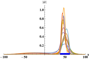
Figure 2: The collapse of the ground state wavefunction when the detector is located at $x=50$ and with half-width $d=10$ lattice units. This run is for $N=1$ and with $r(0)=55$ lattice units. Other parameters are as noted in the text. As time progresses, the wavefunction accumulates at the location of the detector. At time-step 289295, the probability for the particle to be in the detector reaches 0.95. With our chosen time-step, this corresponds to a time of collapse $t_{c}=723.238$ in units of inverse particle mass.

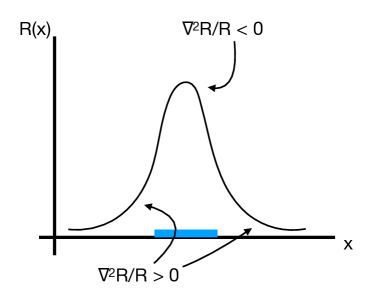
Figure 3: If the wavefunction has a peak within the detector – the horizontal blue line in the sketch – the quantum force given by the last term in Eq. (21) tends to drive the particle realization out of the detector. This is seen by examing the signs of $\nabla^{2}R/R$ at various locations as indicated in the plot. Then the force, which is proportional to $\nabla(\nabla^{2}R/R)$ tends to push the realization out of the detector. This tendency must be overcome by the forces due to the detector potential for the wavefunction to collapse and the particle to be detected.

We can understand the tendency of the realization to stay within the detector in the following way. If we write $\psi(t,x)=R(t,x)\exp(iS(t,x))$, the equation for $S$ is,

$$\partial_{t}S+\frac{(\nabla S)^{2}}{2m}+V_{T}(x)-\frac{1}{2m}\frac{\nabla^{2}R}{R}=0$$ (19)

where $V_{T}$ represents all the potential terms (including for the detector). The velocity of the realization is given by

$${\dot{r}}=\frac{\nabla S(x)}{m}\biggr{|}_{x=r(t)}$$ (20)

and the force on the realization is

$$m{\ddot{r}}=-\nabla V_{T}(x)+\frac{1}{2m}\nabla\left(\frac{\nabla^{2}R}{R}\right)$$ (21)

The first term arises due to the potential well of the detector and tends to keep the realization within the detector. The second term acts in the opposite way and tends to drive the $r(t)$ out of the detector. This is illustrated in Figure 3. The term $-\nabla^{2}R/R$ acts like an additional potential term for the dynamics of $r(t)$. If there is a peak of $R$ within the detector, $-\nabla^{2}R/R>0$ at the peak and $-\nabla^{2}R/R<0$ away from the peak. Hence the additional potential term has a barrier at the peak of the wavefunction and a trough away from the peak. Thus it provides a force on $r(t)$ towards the edges of the detector. If this force can overcome the force due to the detector potential well $V_{T}$, the realization may move out of the detector, leading to the possibility that wavefunction collapse may only occur for “strong detectors”.

The rate of collapse of the wavefunction depends on the location of the detector. In Figure 4 we plot the probability of the particle to be in the detector as a function of time for various locations of the detector. There are oscillations of the probability during the collapse that are most prominent when the detector is placed close to the boundary of the infinite square well.

Figure 4: Plot of the probability to be in the detector versus time-step for various locations of the detector corresponding to Fig. 5. We choose $\lambda=0.01$, $N=1$ and the detector locations range from $x_{0}=0,10,\ldots,80$, with $r(0)=5,15,\ldots,85$ lattice units respectively. The collapse occurs most quickly for detectors placed close to the center of the square well and takes longer for detectors close to the boundaries. The detector at $x_{0}=90$ lattice units is not shown because $r(t)$ quickly moves to the boundary of the square well; the curves for the $x_{0}=0$ and $x_{0}=10$ detectors lie too close to each other to be distinguishable in the plot.

We now turn to the evolution of the particle realization, $r(t)$. This is plotted in Figure 5 for various locations of the detector. Here too we see rapid oscillations in $r(t)$ but the most interesting feature is that $r(t)$ strays out of the detector in which it started but then returns to the detector. This will have important consequences when we consider multiple detectors as in the sections below.

Next we consider the dependence of the collapse on the number of degrees of freedom of the detector, $N$. We fix the position of the detector to be $x_{0}=0$ lattice units and study wavefunction collapse for $N=2,4,6,8,10$ as shown in Figure 6. Increasing $N$ makes the collapse occur more quickly. We quantify this feature in Figure 7 where we plot the collapse time $t_{c}$ versus $N$ on a log-log scale. The straight line indicates a power law,

$$t_{c}\propto N^{-0.38}$$ (22)

This shows that detectors with larger number of internal degrees of freedom make the wavefunction collapse more quickly, in accordance with expectations.

Figure 5: Plot of the realization $r(t)$ vs. time-step for the same parameters and initial conditions as in Fig. 4. For example, the fifth (purple) curve from below corresponds to a detector at $x_{0}=40$ with half-width $10$ lattice units and with $r(0)=45$ lattice units. Although the particle realization is initially inside the detector, it briefly strays out of the detector (to about $x=58$) but then returns to stay trapped within the detector until full collapse occurs.

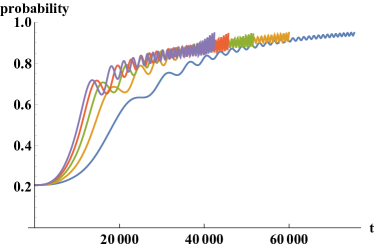
Figure 6: Plot of the probability to be in the detector versus time-step for $N=2$ (blue), 4 (orange), 6 (green), 8 (red), and 10 (purple), for $\lambda=0.01$ when the detector is placed at the center of the square well and $r(0)=5$ lattice units. As $N$ increases the collapse occurs more quickly.

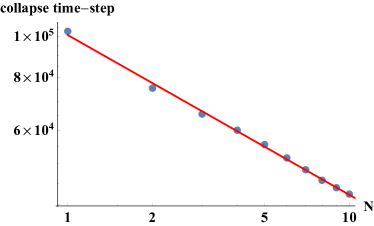
Figure 7: Log-log plot of the time of collapse when the probability to be in the detector reaches 0.95 versus $N$ for $\lambda=0.01$ when the detector is placed at the center of the square well and $r(0)=5$ lattice units. The best fit line is also shown: $y=11.52-0.38x$ and corresponds to an $N^{-0.38}$ fall off of the collapse time with increasing number of degrees of freedom.

II.3 Stochastic $r(0)$

The initial realization, $r(0)$, is a stochastic variable. From the analysis above, if $r(0)$ is inside the detector, then the wavefunction will collapse on to the detector; while if $r(0)$ is outside the detector, then the wavefunction does not collapse and the particle is not detected. Therefore the dBB theory with a single detector will agree with quantum mechanics predictions if the probability density for $r(0)$, denoted $P$, is given by the square of the wavefunction,

$$P[r(0)=r_{0}]=|\psi(0,r_{0})|^{2}$$ (23)

This conclusion applies when the initial wavefunction is in a stationary state. It is not clear to us what distribution of $r(0)$ is appropriate when the initial state is not a stationary state.

III Two detectors

We now consider wavefunction collapse when there are two detectors simultaneously present. The collapse should occur on only one detector and this is indeed what happens as can be seen in Fig. 8. With more than one detector, the evolution of the wavefunction can be affected by the presence of the “dormant” detectors, leading to new dynamics and differences with standard quantum mechanics. For example, if the particle is realized in one detector but meanders into another detector, as seen in Fig. 5, the collapse may occur on the second detector as shown in the bottom right plot of Fig. 8.

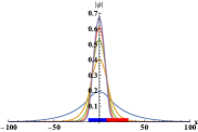
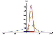
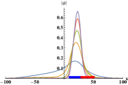
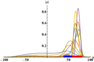
Figure 8: Wavefunction collapse with two detectors in various locations shown by thick blue and red horizontal line segments. (If the detectors are widely separated, the system evolves as in the single detector case.) The model parameters are $\lambda=0.01$ and $N=1$. In the first three cases, the second detector plays no role and the collapse proceeds as if there was only one detector. In the fourth case (bottom right) $r(0)$ is chosen within the left detector, which is also where the wavefunction starts to collapse. However, after some time the collapse shifts to the detector on the right where the particle is eventually detected.

IV Detector array

Now we consider the situation where the square well is lined with an array of 10 detectors that cover $x\in[-L,L]$. We solve equations (14), (15), and (16) as before, scanning over $r(0)$, the initial value of the realization. In each run, the wavefunction collapses on a detector but the collapse onto a detector is affected by the presence of other detectors as we have already seen in the case of two detectors in Sec. III.

Next we factor in the probability distribution of $r(0)$ as in Eq. (23). Thus each initial value of $r(0)$ carries a weight given by the initial probability $|\psi(t=0,r(0))|^{2}$ and we can determine the probability that the wavefunction will collapse on any given detector. Define $S_{n}$ to be the set of $r(0)$ values for which the wavefunction collapses on to the $n^{th}$ detector. Then the probability for collapse on to the $n^{\rm th}$ detector is,

$$p_{n}=\sum_{r_{0}\in S_{n}}P[r_{0}]$$ (24)

The result for $p_{n}$ for each detector is shown in Figure 9 where we compare it to the usual quantum mechanics prediction,

$$p_{n}^{(0)}=\int_{D_{n}}dx\,|\psi(0,x)|^{2}$$ (25)

where the integration is over the extent of the $n^{th}$ detector. We see from Figure 9 that $p_{n}$ is different from $p_{n}^{(0)}$ for $N=1$ and $N=2$. (For the $N=2$ case, the time-dependent potential in (14) is larger and we encountered numerical issues for a handful of values of $r(0)$. So we made our criterion defining collapse less stringent by setting the cutoff probability to count as a collapse to be 0.75 instead of 0.95.) From Figure 9 we see that only the probabilities for the central two detectors in dBB theory agree with quantum mechanics for $N=1$. When we increase $N$ to 2, the agreement improves to the central four detectors. From this trend it appears that probabilities in dBB theory tend towards standard quantum mechanics probabilities as $N$ gets larger and will agree perfectly in the $N\to\infty$ limit. The different probabilities predicted by dBB theory and standard quantum mechanics for smaller values of $N$ may pave the way for an experimental test of dBB theory.

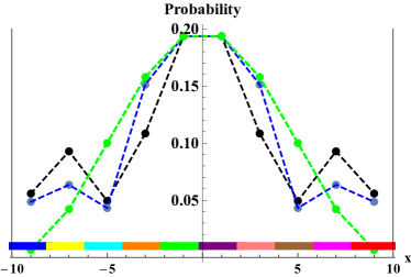
Figure 9: The probability for wavefunction collapse on a detector when there is an array of 10 detectors laid out across the infinite square well. The dBB theory result is shown in black dots joined by the dashed black curve for $N=1$ and by the blue dots and blue dashed curve for $N=2$, though with a lower collapse probability threshold of 0.75 (instead of 0.95) for $N=2$ case for numerical reasons. The probabilities calculated in standard quantum mechanics are shown by the green dots joined by the dashed green curve. The ten detectors are represented by the thick horizontal colored lines.

V Conclusions

In quantum mechanics definite classical realizations of quantum systems are postulated when measurements are made but the quantum to classical transition (wavefunction collapse) is not resolved. In dBB theory, there is a dynamical resolution of wavefunction collapse. We have examined this process in a very specific simple setup. We find dynamical collapse of the wavefunction during a measurement and that the collapse occurs more rapidly with larger number of degrees of freedom of the detector: the collapse time decreases with $N$ as $N^{-0.38}$ as in Figure 7. If the system consists of a single detector, we can postulate a probability distribution of the hidden variable of dBB theory such that the detection probabilities agree with those of standard quantum mechanics. With multiple detectors present, the detection probabilities in dBB theory show departures from standard quantum mechanics as in Figure 9.

The departures from standard quantum mechanics should be a general conclusion for all models in which there is dynamical wavefunction collapse because the wavefunction has to “decide” on which detector to collapse and this can take time during which the dynamics of the wavefunction can be altered. (Departures from quantum mechanics predictions in cosmology have also been studied in a Continuous Collapse Localization model Martin and Vennin (2019a, b).) With dynamical collapse and multiple measuring devices that are each trying to collapse the wavefunction, the detectors can start interfering with each other. We expect that the departures from standard quantum mechanics will become minimal as we go to larger and more complex detectors. An experimental test of dBB theory would be to obtain detection probabilities when there are multiple, small detectors present in the experimental setup.

Our analysis has been restricted to a very simple and idealized system. It is important to extend the analysis to more realistic systems. It would also be useful to apply a similar analysis to discrete (spin) systems and to see if they can provide an experimental test of dBB theory. Finally, it remains to be seen if an analogous system can be set up in field theory in terms of a wavefunctional and a classical realization of the field.