Reconstruction of moiré lattices in twisted transition metal dichalcogenide bilayers

Abstract

An important step in understanding the exotic electronic, vibrational, and optical properties of the moiré lattices is the inclusion of the effects of structural relaxation of the un-relaxed moiré lattices. Here, we propose novel structures for twisted bilayer of transition metal dichalcogenides (TMDs). For $\theta\gtrsim 58.4^{\circ}$, we show a dramatic reconstruction of the moiré lattices, leading to a trimerization of the unfavorable stackings. We show that the development of curved domain walls due to the three-fold symmetry of the stacking energy landscape is responsible for such lattice reconstruction. Furthermore, we show that the lattice reconstruction notably changes the electronic band-structure. This includes the occurrence of flat bands near the edges of the conduction as well as valence bands, with the valence band maximum, in particular, corresponding to localized states enclosed by the trimer. We also find possibilities for other complicated, entropy stabilized, lattice reconstructed structures.

The formation of flat bands in the electronic band structure of moiré patterns of two-dimensional materials is central to understanding the observed exotic electronic phases Bistritzer and MacDonald (2011); Cao et al. (2018a, b); Yankowitz et al. (2019). Twisted bilayer TMDs can possess flat bands for a continuum of twist angles Naik and Jain (2018); Naik et al. (2019a); Fleischmann et al. (2019); Wang et al. (2020); Zhang et al. (2019); Wu et al. (2019); Bi et al. (2019); Angeli and MacDonald (2020); Pan et al. (2020); Zhan et al. (2020); Zhai and Yao (2020). To accurately calculate their electronic band structure, incorporation of structural relaxation effects is crucial Naik et al. (2019a); Gargiulo and Yazyev (2017); Yoo et al. (2019); Naik and Jain (2018); Lucignano et al. (2019); Nam and Koshino (2017); Leconte et al. (2019); Halbertal et al. (2021). Typically, these relaxations are performed by starting from a configuration and only allowing downhill motion in the potential energy landscape using local search algorithms (standard minimization). Since the number of local minima in the potential energy landscape increases exponentially with the number of atoms, standard minimizations are often insufficient for finding the stable structuresPickard and Needs (2011); Stillinger (1999); Kirkpatrick et al. (1983). All the studies conducted on moiré materials to date presume that the moiré lattice constant of the un-relaxed twisted structure remains intact even after relaxation. Bistritzer and MacDonald (2011); Cao et al. (2018a, b); Yankowitz et al. (2019); Naik and Jain (2018); Naik et al. (2019a); Fleischmann et al. (2019); Wang et al. (2020); Zhang et al. (2019); Wu et al. (2019); Gargiulo and Yazyev (2017); Yoo et al. (2019); Lucignano et al. (2019); Nam and Koshino (2017); Carr et al. (2018); Enaldiev et al. (2020); Weston et al. (2020); Rosenberger et al. (2020); Leconte et al. (2019).

Here, from the structures obtained using simulated annealing we demonstrate that a dramatic reconstruction of moiré lattices of TMDs takes place for $\theta\gtrsim 58.4^{\circ}$. Thus, the presumption that the moiré lattice constant of the rigidly twisted structures continues to characterize the relaxed structures is not always valid. Such lattice reconstructions are not accessible in standard minimization approaches. We discuss below the details of the lattice reconstruction for twisted bilayer (tBL) of $\mathrm{MoS_{2}}$. We have also verified our conclusions for $\mathrm{MoSe_{2},\ WSe_{2},\ WS_{2}}$ (see Supplementary Information (SI), Sec. II SI ). We demonstrate that the lattice reconstruction substantially changes the electronic band structure.

We use the TWISTER code Naik and Jain (2018) to construct tBLTMDs. We use the Stillinger-Weber and Kolmogorov-Crespi (KC) potential to capture the intra and interlayer interaction of tBLTMDs, respectively Jiang and Zhou (2017); Naik et al. (2019b). The used KC parameters have been shown to accurately capture the interlayer van der Waals interaction present in the TMDs Naik et al. (2019b). We relax the tBLTMDs in LAMMPS using standard minimization Plimpton (1995); Bitzek et al. (2006), denoted as standard relaxation (SR). We also perform classical molecular dynamics simulations using the canonical ensemble at $T=1$ K and cool down snapshots to 0 K, and then carry out an energy minimization. We refer to this second approach as simulated annealing (SA). The phonon frequencies are calculated using modified PHONOPYTogo and Tanaka (2015) code. We perform electronic structure calculations using density functional theoryKohn and Sham (1965) with SIESTA Lin et al. (2014); Soler et al. (2002); zhe Yu et al. (2018); Lin et al. (2009); Troullier and Martins (1991); Dion et al. (2004); Cooper (2010); van Setten et al. (2018) (SI Sec. I for details SI ).

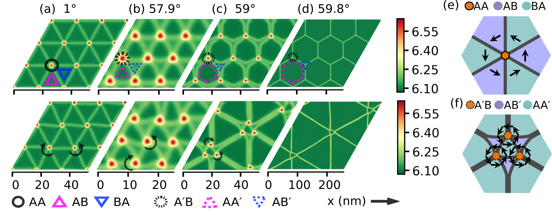
Figure 1: (a)-(d): Interlayer separation landscape of $\mathrm{tBLMoS_{2}}$ using standard relaxation (top panel) and simulated annealing (bottom panel). The smallest repetitive cell in the top panel is a moiré unit cell. The scales of the colorbar, in Å and corresponds to interlayer separation. The curling of domain walls near a few $\mathrm{AA,\ A^{\prime}B}$ stackings are marked. (e),(f): Schematics near the topological defects for $\mathrm{tBLTMDs}$ for $\theta=1^{\circ},\ 59^{\circ}$, respectively. The order parameter is shown with arrows.

Due to the presence of different sub-lattice atoms (Mo/W, S/Se) in TMD, the tBLTMD possesses distinct high-symmetry stackings for $\theta$ near $0^{\circ}$ ($\mathrm{AA,\ AB,\ BA}$) and near $60^{\circ}$ ($\mathrm{AA^{\prime}\ ,AB^{\prime},\ A^{\prime}B}$) Liang et al. (2017). Nevertheless, the lattice constants of the un-relaxed tBL are identical for $\theta$ and $60^{\circ}-\theta$ (e.g. $1^{\circ}$ and $59^{\circ}$). Among the above mentioned stackings, $\mathrm{AB}$ is energetically the most favourable stacking as $\theta\to 0^{\circ}$ ($E_{\mathrm{AB}}=E_{\mathrm{BA}}<E_{\mathrm{AA}}$, six-fold symmetric around $\mathrm{AA}$) and $\mathrm{AA^{\prime}}$ for $\theta\to 60^{\circ}$ ($E_{\mathrm{AA^{\prime}}}<E_{\mathrm{AB^{\prime}}}<E_{\mathrm{A^{\prime}B}}$, three-fold symmetric around $\mathrm{A^{\prime}B}$) Naik et al. (2019b); Carr et al. (2018).

In Fig. 1 we show the interlayer separation (ILS) landscape for a $3\times 3\times 1$ moiré supercell of $\mathrm{tBLMoS_{2}}$, obtained using both SR and SA. The landscape for $\theta=1^{\circ}$ is a representative of $\theta\to 0^{\circ}$ (Fig. 1a, top panel). With SR we find straight domain walls separating AB, BA stackings. On the other hand, the ILS landscape computed with SA shows a slight curling of the domain walls near AA stacking (Fig. 1a, bottom panel). Although the number of clockwise and counter-clockwise curlings are equal, they do not always form a checkerboard-like pattern. While the checkerboard pattern is the lowest in energy, the energy difference between the checkerboard pattern and a random distribution of curlings is small (a few meV per moiré lattice). Nevertheless, the AA stackings always form a triangular lattice for any $\theta$ close to $0^{\circ}$, consistent with experiments Weston et al. (2020); Rosenberger et al. (2020); Zhang et al. (2019).

In contrast, the behavior of the ILS landscape shows very different, and intriguing features as $\theta\to 60^{\circ}$. We categorize the $\theta$ dependence into two regions. Region I ($\theta<58.3^{\circ}$) : With SR both the $\mathrm{AA^{\prime}}$ and $\mathrm{AB^{\prime}}$ stackings occupy comparable areas of the supercell, with each forming an approximate equilateral triangle (Fig. 1b). Similar to $\theta\to 0^{\circ}$, the ILS landscape obtained with SA shows curlings of domain walls near $\mathrm{A^{\prime}B}$ stacking (Fig. 1b, bottom panel). Region II ($\theta\gtrsim 58.4^{\circ}$) : The most favorable ($\mathrm{AA^{\prime}}$) stacking increases in area significantly and evolves from Reuleaux triangles to approximate hexagonal structures, as obtained with SR (Fig. 1c-d, top panel), consistent with previous studies Carr et al. (2018); Enaldiev et al. (2020). In this case, the domain walls connecting $\mathrm{A^{\prime}B}$ stackings are significantly curved and never straight-lines. These latter structures show notable reconstruction with SA. In particular, a triangular lattice is formed with three $\mathrm{A^{\prime}B}$ stackings trimerizing to form a motif (Fig. 1c-d, bottom panel). Moreover, the domain walls connecting different $\mathrm{A^{\prime}B}$ stackings are almost straight in the reconstructed structures. The reconstructed structures obtained using SA are always energetically more stable than those obtained using SR.

We characterize the domain walls using the order-parameter, defined as the shortest displacement vector required to take any stacking to the most unfavorable stacking Alden et al. (2013); Naik and Jain (2018); Gargiulo and Yazyev (2017). Irrespective of $\theta$, we find the domain walls to be shear solitons (change in order parameter is along the domain wall as we go from $\mathrm{AB}\to\mathrm{BA}$ for $\theta\to 0^{\circ}$ and $\mathrm{AA^{\prime}}\to\mathrm{AA^{\prime}}$ for $\theta\to 60^{\circ}$). In Region II, two domain walls come close together and the effective width increases. For $\theta\to 0^{\circ}$ ($\theta\to 60^{\circ}$), the calculated widths of the domain walls are : 2.9 (4.3) for $\mathrm{tBLMoS_{2}}$, 2.9 (3.8) for $\mathrm{tBLMoSe_{2}}$, 3.7 (4.7) for $\mathrm{tBLWSe_{2}}$, 3.5 (4.5 ) for $\mathrm{tBLWS_{2}}$ ( all in nm). Our estimated domain wall widths are in good agreement with experiment Weston et al. (2020). Moreover, the order parameter rotates by $2\pi$ at $\mathrm{AA/A^{\prime}B}$, indicating it’s topological nature (Fig. 1e, 1f). We do not find any new creation or annihilation of the topological defects and domain walls in our simulations.

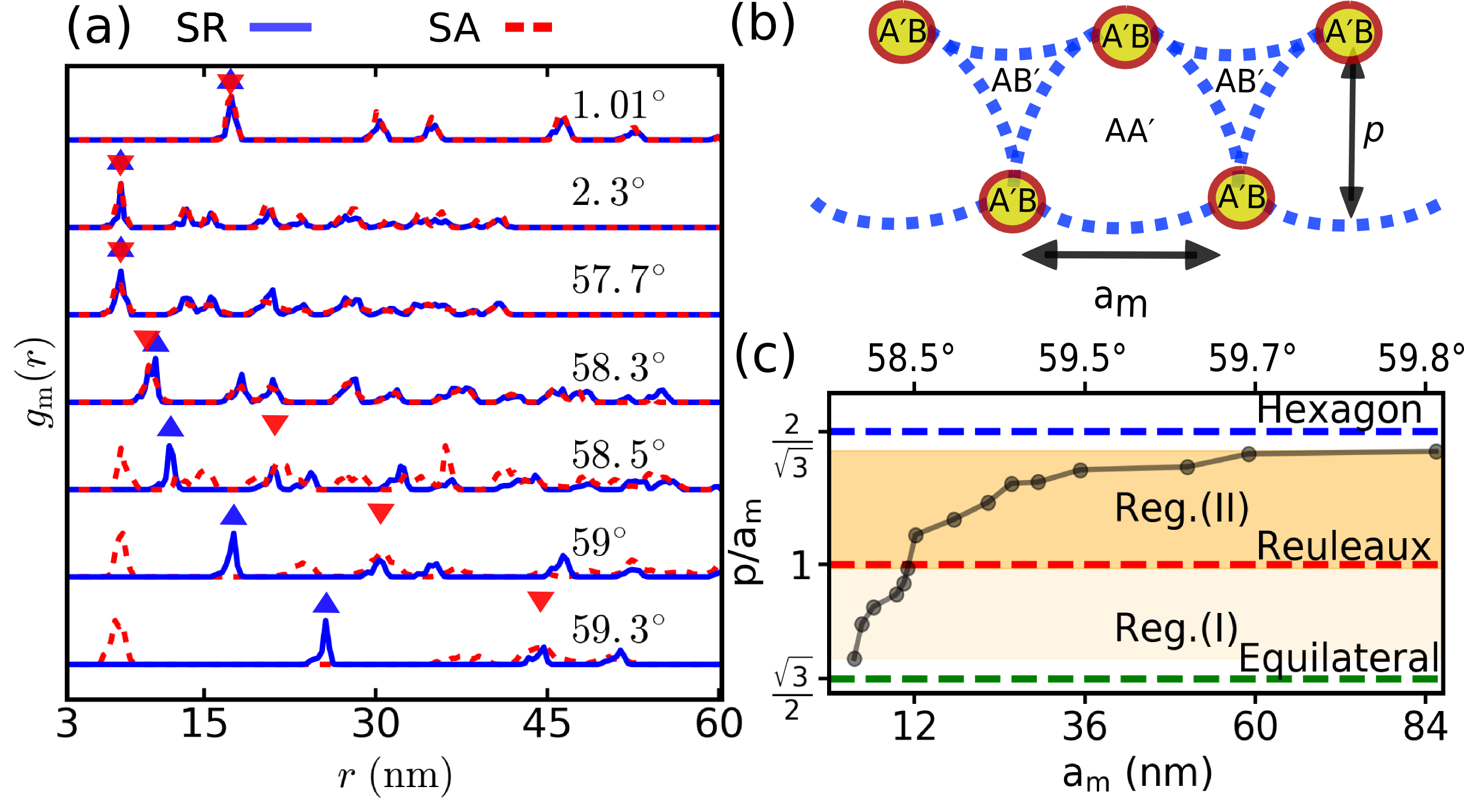
Figure 2: (a) Radial distribution function, $g_{\mathrm{m}}(r)$ computed with standard relaxation (SR) and simulated annealing (SA). The moiré lattice constants are marked (blue triangle pointing up for SR, red triangle pointing down for SA). (b) Schematics of $\mathrm{tBLMoS_{2}}$ as $\theta\to 60^{\circ}$ with SR. (c) Change of $p/\mathrm{a_{m}}$ with $\mathrm{a_{m}}$. Several ideal geometric structures are marked with dashed lines.

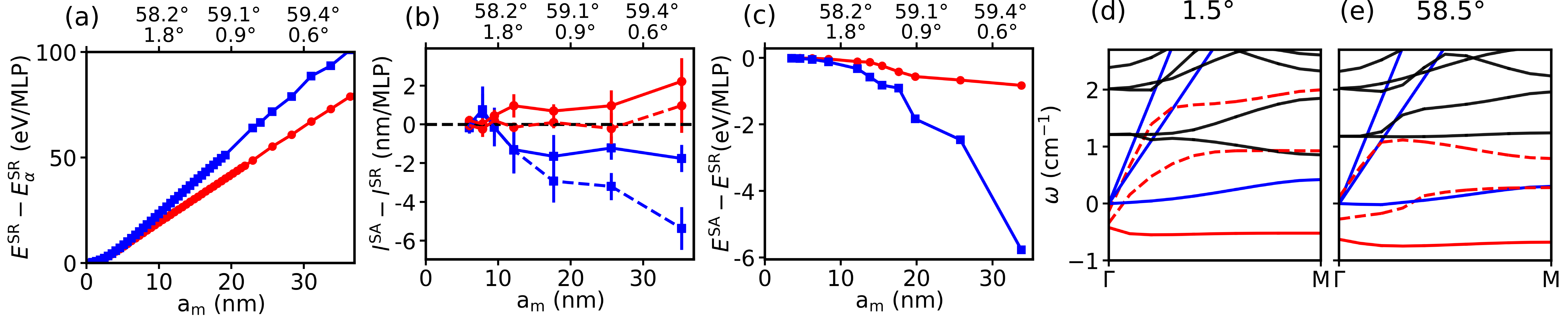
Figure 3: (a) Change of total energy computed with respect to stable stacking, $\alpha$ using SR with $\mathrm{a_{m}}$ (corresponding $\theta$ are marked; blue (red) for near $60^{\circ}$ ($0^{\circ}$) for (a)-(c)). (b) Change in domain wall length with SA compared to SR excluding (dashed lines) and including (solid lines) curling near $\mathrm{AA/A^{\prime}B}$. The error bar denotes standard deviation of the estimated change. (d) Total energy gain with SA compared to SR. (d),(e) Phonon dispersion with SR for $1\times 1\times 1$ moiré cell. The solid blue, dashed red, solid red lines represent the acoustic, phason, buckling mode localized at $\mathrm{AA/A^{\prime}B}$, respectively.

We investigate the structural long-range order by computing the radial distribution function. In the $\mathrm{tBL}$ there are two distinct length scales, one for the individual TMD layer given by the lattice constant $a$, and the other for the moiré lattice given by the $\theta$ dependent moiré lattice constant, $\mathrm{a_{m}}=a/(2\sin(\theta/2))$. Therefore, we define two separate radial distribution functions, one for atoms of the individual layers and another for stackings of the moiré lattice. We compute the moiré-scale radial distribution function, $g_{\mathrm{m}}(r)$ using the $\mathrm{AA/A^{\prime}B}$ stackings of $\mathrm{tBLMoS_{2}}$ (Fig. 2a). Each $\mathrm{AA/A^{\prime}B}$ stacking represents a moiré lattice point (MLP).

For $\theta\to 0^{\circ}$, $g_{\mathrm{m}}(r)$ obtained using SR and SA are similar (Fig. 2a). The average number of nearest neighbour MLPs is always 6, calculated by integrating the first peak of $g_{\mathrm{m}}(r)$. This confirms the existence of the hexagonal network formed by domain walls (Fig. 1a). Furthermore, the moiré lattice constant calculated from $g_{\mathrm{m}}(r)$ is identical to that of un-relaxed $\mathrm{tBLMoS_{2}}$. Therefore, the long-range order of the un-relaxed structures remains intact as $\theta\to 0^{\circ}$. As $\theta\to 60^{\circ}$ within Region I, the moiré lattice constants are again identical for un-relaxed and relaxed structures, $\mathrm{a_{m}=a_{m}^{SR}=a_{m}^{SA}}$ (Fig. 2a), and the number of nearest neighbour MLP is always 6. In contrast, the lattice reconstruction in Region II leads to the formation of a triangular lattice with a modified lattice constant, $\mathrm{a_{m}^{SA}=\sqrt{3}a_{m}}$ (Fig. 2a). The first peak in the $g_{\mathrm{m}}(r)$ ($\approx 7.5$ nm) corresponds to the motif of the triangular lattice. The motif consists of 3 $\mathrm{A^{\prime}B}$ stackings. We find that the number of the nearest neighbor of $\mathrm{A^{\prime}B}$ is 2. We also examine the atomic radial distribution function for individual $\mathrm{MoS_{2}}$ layers. Irrespective of $\theta$, the long-range order is preserved at the unit-cell $\mathrm{MoS_{2}}$ scale. This establishes that the aforementioned reconstruction in Region II is an emergent phenomenon arising at the moiré-scale.

To pinpoint the onset of the lattice reconstruction geometrically, we consider the ratio of the perpendicular bisector, $p$, to $\mathrm{a_{m}}$ of $\mathrm{tBLMoS_{2}}$ obtained using SR (Fig. 2b). Interestingly, we find lattice reconstruction as $p/a_{\mathrm{m}}$ becomes $\gtrsim 1$ (Fig. 2c). When $p/\mathrm{a_{m}}=1$ ($\theta\sim 58.5^{\circ}$), the $\mathrm{AA^{\prime}}$ stacking represents a Reuleaux triangle with the domain walls occupying it’s perimeter. When one considers the perimeter² to area ratio, the Reuleaux triangle is a local maximum Modes and Kamien (2013). Since the domain walls are energetically unfavorable compared to $\mathrm{AA^{\prime}}$, the Reuleaux triangle is expected to undergo rearrangements to minimize the total energy. The shortest distance between two $\mathrm{A^{\prime}B}$ stackings is $\approx d^{\mathrm{A^{\prime}B}}+d^{\mathrm{AB^{\prime}}}\approx 3.3+4.5=7.8$ nm, where $d^{\mathrm{A^{\prime}B}},d^{\mathrm{AB^{\prime}}}$ denote the sizes of the corresponding stackings. This explains the occurrence of first peak in $g_{\mathrm{m}}(r)$ in Region II at $\approx 7.5$ nm.

Next, we investigate the origin of these reconstructions from energetics. The total energy of the $\mathrm{tBLMoS_{2}}$ is a sum of the intralayer energy, which is a combination of strain and bending energy Maity et al. (2018), and the interlayer energy. For $\theta\to 60^{\circ}$, the interlayer energy per MLP can be approximated as,

$$E_{\mathrm{inter}}-E_{\mathrm{inter}}^{\mathrm{AA^{\prime}}}=\delta E^{\mathrm{A^{\prime}B}}_{\mathrm{inter}}S^{\mathrm{A^{\prime}B}}+\delta E^{\mathrm{DW}}_{\mathrm{inter}}S^{\mathrm{DW}}+\delta E^{\mathrm{AB^{\prime}}}_{\mathrm{inter}}S^{\mathrm{AB^{\prime}}}$$ (1)

Here, $\delta E^{\alpha}_{\mathrm{inter}}$ represents the interlayer energy of stacking $\alpha$, evaluated with respect to $\mathrm{AA^{\prime}}$ and $S^{\alpha}$ denotes the occupied area. For small $\theta$, $S^{\mathrm{A^{\prime}B}},\ S^{\mathrm{AB^{\prime}}}$ and the width of the domain wall (DW), $w$, become constant ($S^{\mathrm{DW}}=wl$). Therefore, the interlayer energy as in Eqn.(1) becomes linear with the domain wall length, $l$, and is repulsive. Moreover, the intralayer strain energies are concentrated on the domain walls and scales as $l/w$ Alden et al. (2013); Zhang and Tadmor (2018). Thus, the minimization of $l$ will minimize both the interlayer and intralayer energies. In Fig. 3a we show the scaling of the total energy with $\mathrm{a_{m}}$ using SR. The domain walls obtained with SR are always significantly curved for $\theta>58.4^{\circ}$. The lengths of these curved domain walls can be minimized by lattice reconstruction such that the domain walls become straightlines (as in Fig. 1c,1d, bottom panel). On the other hand, the domain walls are straightlines for the corresponding set of $\theta$ near $0^{\circ}$ with SR. Thus, $l$ per moiré lattice is already minimized. As a result, we do not find lattice reconstruction with SA as $\theta\to 0^{\circ}$. However, the domain walls obtained with SA are always curled near the $\mathrm{AA,\ A^{\prime}B}$ stackings, irrespective of lattice reconstruction. This originates from a buckling instability, primarily localized at $\mathrm{AA,A^{\prime}B}$ (see below). Taking these into account, $l^{\mathrm{SA}}$ is expected to be greater than $l^{\mathrm{SR}}$ in the absence of lattice reconstruction. In Fig. 3b we show the estimate of $(l^{\mathrm{SA}}-l^{\mathrm{SR}})$ per MLP as $\theta\to 0^{\circ},\ \to 60^{\circ}$ (see SI, Sec. III for details). For $\theta\gtrsim 58.4^{\circ}$, the difference becomes negative, indicating a reduction in the domain wall length for the reconstructed lattice. The reduction in $l$, disregarding the curling of the domain walls with SA, is large in Region II (Fig. 3b). Fig. 3c shows the gain in total energy with SA relative to SR, which is significantly greater in Region II than that for a corresponding $\theta$ near $0^{\circ}$ . The energy gain near $0^{\circ}$ arises from curling of the domain walls near $\mathrm{AA}$, whereas the gain in Region II arises predominantly from lattice reconstruction.

We also compare the low-frequency vibrational modes of $1.5^{\circ}$ and $58.5^{\circ}$ tBL$\mathrm{MoS_{2}}$. One of the phason modes Maity et al. (2020) softens significantly and becomes nearly dispersion-less with attributes of a zero mode for $58.5^{\circ}$ (Fig. 3d, 3e). Such a mode is expected to cause reconstruction of lattices Sun et al. (2012). Furthermore, with SR we find a soft mode with imaginary frequency for both $1.5^{\circ}$ and $58.5^{\circ}$ (Fig. 3d, 3e). The corresponding eigenvector at $\Gamma$, which is localized on $\mathrm{AA/A^{\prime}B}$, denotes a buckling instability and can be removed without lattice reconstruction.

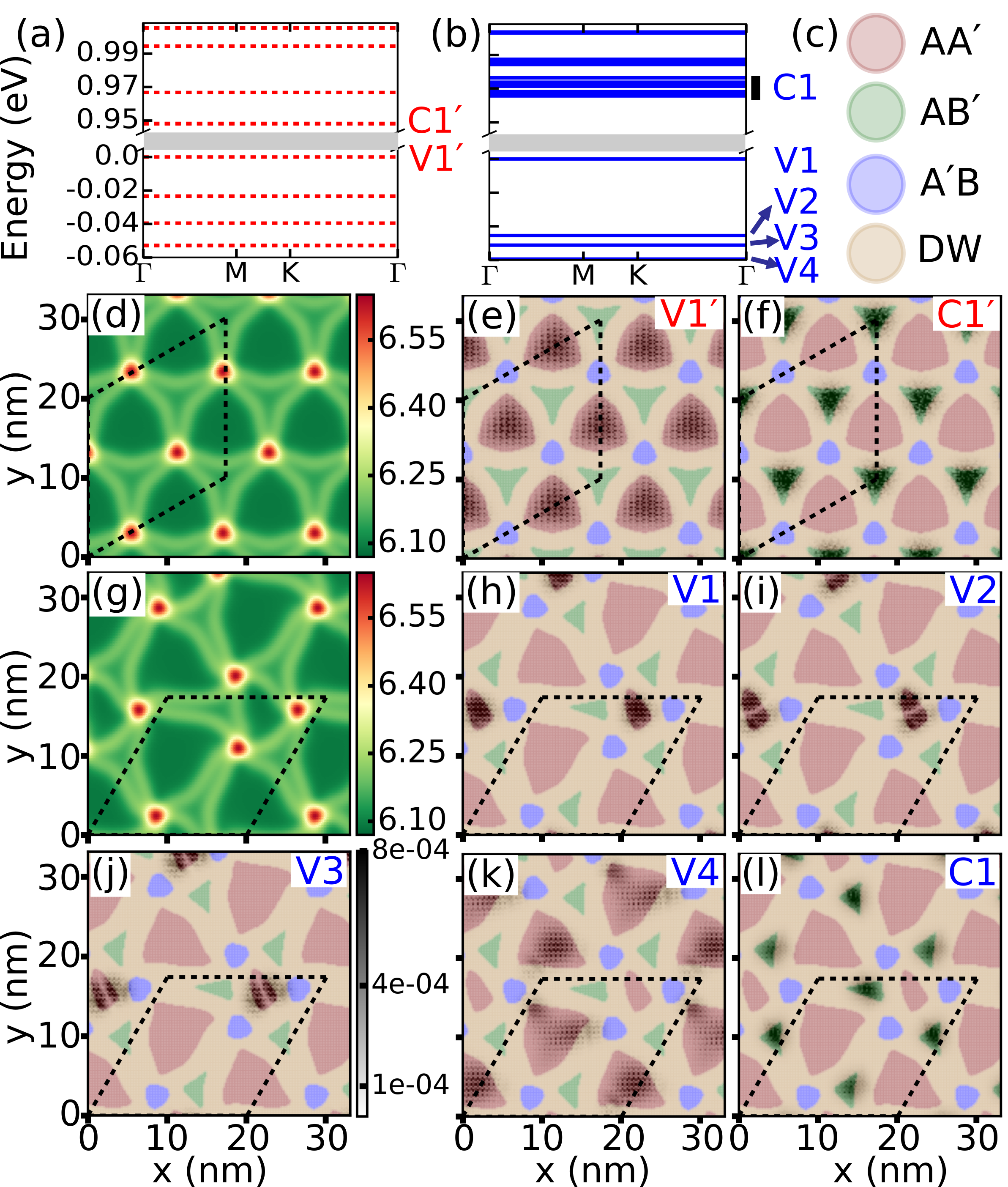
Figure 4: (a),(b) Electronic band structures near the band edges of a $\sqrt{3}\times\sqrt{3}\times 1$ supercell of $\mathrm{tBLMoS_{2}}$ for $58.47^{\circ}$ with SR and SA, respectively. The supercell is marked with black dashed lines. (c) Colors used to denote stackings in (e)-(f),(h)-(l). (d),(g) ILS landscape for $58.47^{\circ}$ with SR and SA, respectively. $|\psi_{\Gamma}(\vec{r})|^{2}$ averaged in the out-of-plane direction of the states near VBM, and near CBM for structures obtained with SR ((e)-(f)) and with SA ((h)-(l)) with the corresponding colorbar shown in (j). A linear combination is shown in (l) as C1 corresponding to bands marked in (b).

During our simulations we find transient structures, such as, distorted hexagon, kagome, etc, which evolve to form the structures shown in Fig 1c,d (SI, Sec. IV). To investigate entropic effects, we also simulate a supercell with 100 moiré lattices allowing significantly large degrees of freedom for lattice reconstruction. We find that lattice reconstructed structures with motifs of $>3$ $\mathrm{A^{\prime}B}$ stackings, nonuniform hexagons with parallel domain walls are also possible (SI, Sec. IV). These structures can be metastable due to the presence of a substrate, strain, etc in an experiment. These external effects can modify the characteristic angle for the onset of lattice reconstruction. Our study suggests that the highly non-uniform hexagons with complex domain wall structures found in the experiments Weston et al. (2020); Rosenberger et al. (2020) are closely connected to the intrinsic lattice reconstruction. The “breathing” of hexagons in a hexagonal network of domain walls can give rise to distorted hexagons and carry large entropy Riste (2012). Our calculations suggest that these effects are realized for a general class of domain wall networks in moiré materials (Reuleaux triangle to hexagons).

In Fig. 4a-b we compare the electronic band structures of $\mathrm{tBLMoS_{2}}$ obtained for $58.47^{\circ}$, which contains 24966 atoms. The lattice reconstruction leads to an increment in the band-gap by $\sim 20$ meV and significant changes in the spacing of energy levels near the band edges. Interestingly, we find the bands are ultra-flat (bandwidth $\lessapprox 1$ meV within DFT) near the band-edges for both the structures obtained with SR and SA. However, the wave-function localizations corresponding to these flat bands are strikingly different. To illustrate this, we show the density associated with the first few-bands near the band edges. With SR, the states near the valence band maximum (VBM) resemble the states of a particle confined in a two dimensional equilateral triangular well and are localized on $\mathrm{AA^{\prime}}$ (Fig. 4c,4e) Naik et al. (2019a). In the reconstructed lattice, the degeneracies associated with the equilateral triangular well are lifted, as triangles of various shapes and depths are realized. In particular, the wave functions corresponding to first three bands near the VBM are localized on the $\mathrm{AA^{\prime}}$ stacking enclosed by the trimer (Fig. 4h-j), whereas for the fourth band, the wave function is localized on the larger $\mathrm{AA^{\prime}}$ stackings (Fig. 4k). Since the area enclosed by the trimer in the reconstructed lattice (Fig. 4d) is $\theta$ independent, the spatial extension of the localized VBM is expected to be $\theta$ independent. The states near the conduction band minimum (CBM) are localized on the $\mathrm{AB^{\prime}}$ stacking (Fig. 4f, 4l), whose size is also $\theta$ independent. This explains the experimentally observed large tunnelling current at $\mathrm{AB^{\prime}}$ Weston et al. (2020); Rosenberger et al. (2020). The distinct spatial localizations of electrons and holes originate from an in-plane strain driven moiré potential Naik et al. (2019a). For the un-reconstructed lattice, the height of the moiré potential is identical at all $\mathrm{AA^{\prime}}$ stackings ($\approx 132$ meV). After lattice reconstruction, the height of the moiré potential at $\mathrm{AA^{\prime}}$ enclosed by the trimer is maximal ($\approx 171$ meV) and at other $\mathrm{AA^{\prime}}$ stackings is unmistakably smaller ($\approx 98$ meV) (SI, Sec. V for details). The depth of the moiré potential at $\mathrm{AB^{\prime}}$ also changes after lattice reconstruction ($\approx-306$ with SR and $\approx-255$ with SA, in meV). Furthermore, we have also obtained fully relaxed structures with SR and SA using DFT calculations for a $\sqrt{3}\times\sqrt{3}\times 1$ supercell of 58.53^∘ tBLMoS₂. After applying a small ($s>1.5\%$ )compressive strain, we show that the lattice reconstructed structures obtained from SA are more stable (SI, Sec. VI).

We have demonstrated reconstruction of the moiré lattices of TMDs for $\theta>58.5^{\circ}$. These structures can be probed using electron microscopy, optical imaging, etc., and are expected to be generic for tBLs with different sub-lattice atoms, including TMD heterostructures Alden et al. (2013); Yoo et al. (2019); Weston et al. (2020); Rosenberger et al. (2020); Zhang et al. (2018); Xu et al. (2020); Andersen et al. (2019); Scuri et al. (2020); Baek et al. (2020); Ni et al. (2019); Jiang et al. (2016); Holler et al. (2020); Gadelha et al. (2020).

Supplementary Information:
Reconstruction of moiré lattices in twisted transition metal dichalcogenide bilayers

Indrajit Maity, Prabal K. Maiti, H. R. Krishnamurthy

Manish Jain

I I: Simulation details

Classical force-field based calculations:
(A) Details of structural relaxation: The standard relaxation (SR) is performed with the target pressure of P = 0 bar. For the simulated annealing (SA), the simulation box dimensions were kept the same as in SR. We use Nosé-Hoover thermostat while performing simulations with canonical ensemble. It should be noted that annealing at higher temperatures ($>1$ K) produces results similar to the ones discussed in the main text. In total, we have simulated $\sim 70$ twist angles ($\sim 40$ of them near $60^{\circ}$ and $\sim 30$ of them near $0^{\circ}$ ), with systems containing $10^{5}-10^{7}$ atoms, within the twist angle range, $0.2^{\circ}\leq\theta\leq 59.8^{\circ}$. For total energy comparisons as in Fig.3 of main text we use energy tolerance of $10^{-11}$ to perform the relaxation.

(B) Details of phonon calculations: While computing the phonon frequencies we have used force tolerance of $10^{-6}$ eV/Å for the results presented in the main text. The relaxed structures are obtained by SR method.

(C) Radial distribution function: The radial distribution function at the moiré scale, $g_{\mathrm{m}}(r)$ is computed with $9\times 9\times 1$ moiré supercell and averaged over 30 configurations. After performing molecular dynamics on a $3\times 3\times 1$ supercell, we replicate the structure to further create $9\times 9\times 1$ supercell and perform molecular dynamics. Identifying the moiré lattice points (MLPs) corresponding to $\mathrm{AA/A^{\prime}B}$ from the interlayer separation (ILS) landscape, we calculate the $g_{\mathrm{m}}(r)$ defined as, $\frac{\langle N(r+\delta r)\rangle}{A(\delta r)}$ with $\langle N(r+\delta r)\rangle$ representing the average number of MLPs within a ring of radius $r$, width $\delta r$ and the area $A(\delta r)$.

Quantum simulations: We use a double-$\zeta$ plus polarization basis for the expansion of wavefunctions. For all the electronic structure calculations we use the $\Gamma$ point in the moiré Brillouin zone to obtain the converged ground state charge density. A large vacuum spacing of $\sim 40$ Å is used in the out-of-plane direction for all the density functional theory (DFT) calculations. We use a plane wave energy cut-off of 80 Ry to generate the 3D grid for the simulation. To check the adequacy of the effects of the small energy cut-off, we also simulate a $\mathrm{tBLMoS_{2}}$ with large twist angle ($50.6^{\circ}$, 222 atoms) using this cutoff as well as a larger cut-off of 320 Ry. We find a negligibly small difference in the electronic band structures (obtained with the two different cut-offs 320 Ry and 80 Ry). We do not include spin-orbit coupling in our DFT calculations. To study the effects of lattice reconstruction on electronic structure of the twisted bilayer $\mathrm{MoS_{2}}$ we simulate a $\sqrt{3}\times\sqrt{3}\times 1$ moiré supercell for $\theta=58.47^{\circ}$, which contains 24966 atoms. On this supercell, we perform SR (which does not show lattice reconstruction i.e. moiré periodicity of unrelaxed structure is preserved) and SA (which shows lattice reconstruction leading to trimerization i.e. moiré periodicity of un-relaxed structure is not preserved), as described in the main text. We perform electronic structure calculations in two ways:

(D) Multiscale simulations: We use the relaxed structures obtained with accurate classical force-field based simulations and carry out DFT calculations. In this approach, we do not further relax the structures, and local density approximation is used for the exchange-correlation functional. We employ the norm-conserving pseudopotentials Troullier and Martins (1991). This approach critically depends on the accuracy of the classical force-fields. The interlayer classical forcefield parameters were obtained by fitting the interlayer binding energy landscape obtained from the van der Waals corrected DFT calculations Naik et al. (2019b). This multiscale approach is widely used in predicting the electronic properties of the moié materials Naik et al. (2019b, a). All the electronic structure calculations reported in the main text (Fig. 4, for example) are obtained with this approach unless otherwise specified.

(E) Relaxation using DFT: We use the relaxed structures obtained with classical simulations as a starting configuration and further perform relaxation with DFT. In this approach, we use van der Waals density functional that includes a non-local energy functional Dion et al. (2004) alongside Cooper exchange Cooper (2010) as implemented in SIESTA. We employ norm-conserving, scalar relativistic pseudopotential obtained from PseudoDojo van Setten et al. (2018). The relaxations with DFT are performed with 100 meV/Å as the maximum atomic force tolerance for any atom. It should be noted that we use a relatively large atomic force tolerance as the system under consideration contains 24966 atoms. However, we find only a small fraction of atoms ($\approx 0.6\%$) has atomic forces greater than 40 meV/Å in the fully relaxed structure. The atomic force tolerance of 40 meV/Å is the default in SIESTA. Therefore, we expect the ordering of total energetics as shown in table 5 to be reliable. All the related structural relaxation calculations are performed with 4800 cores on a CRAY XC40 machine over 100 days’ worth of computing (total: 4,80,000 core-hours) using SIESTA.

We obtain the ground state charge density using convergence criteria on both densities (with a tolerance of $10^{-4}$) and Hamiltonian (with a tolerance of $10^{-3}$ eV). We use the recently developed Pole Expansion, and Selected Inversion (PEXSI) technique Lin et al. (2009); zhe Yu et al. (2018); Lin et al. (2014) to construct the ground state charge density of large systems. This enables us to perform full DFT relaxation and compute the electronic properties of large-scale moiré patterns of TMDs within a reasonable time. We use the obtained ground state charge density and diagonalize to compute the electronic band-structure. We have also computed the ground-state charge density using standard diagonalization techniques and computed the electronic structure of $\sqrt{3}\times\sqrt{3}\times 1$ lattice reconstructed structures. We find negligibly small differences in the electronic properties between these two approaches.

II II : Reconstruction of moiré lattices for other TMDs

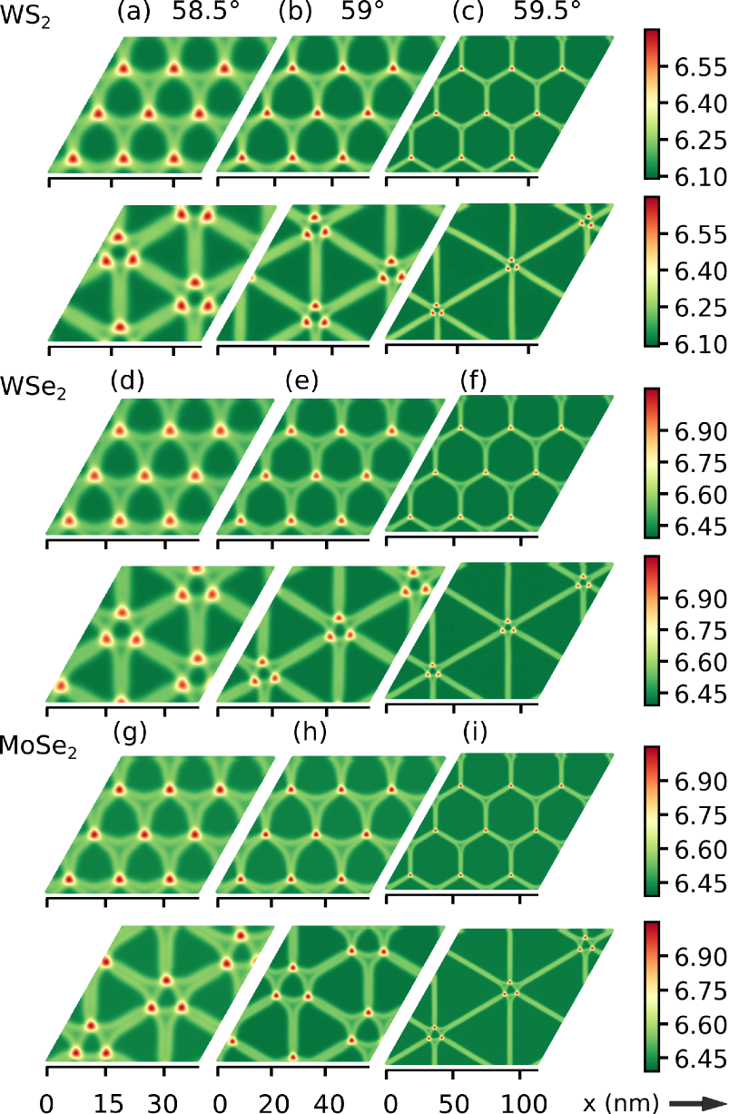
Figure S1: Interlayer separation landscape for for $\mathrm{WS_{2}\,WSe_{2},\ MoSe_{2}}$ using standard relaxation (upper panel for each material) and simulated annealing (lower panel for each material) computed with a $3\times 3\times 1$ moiré supercell. The scales of the associated colorbars are for the interlayer separation in Å.

III III : Estimation of domain wall length

The estimation of the domain wall length, $l$ is done in four steps : (i) Identifying approximately the regions exclusively belonging to the domain walls (ii) Defining a polygon that encloses all the points for a representative domain wall (iii) Finding a suitable representation of the thick domain wall as a line. (iv) Averaging over the supercell to get statistically significant results. We illustrate this in Fig. S2.

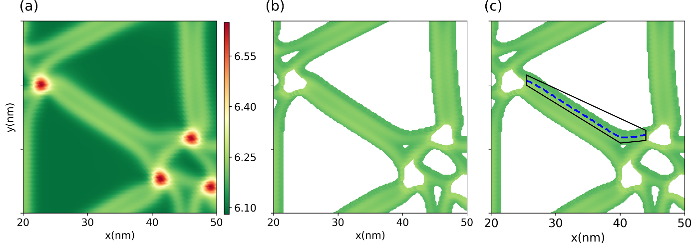
Figure S2: (a) Interlayer separation landscape using the simulated annealing approach for $\theta=59^{\circ}$. The scales of the associated colorbar are for the interlayer separation in Å. (b) Identification of the domain wall region from ILS landscape (c) Defining the polygon (solid black line) and finding a suitable representation of the domain wall (dashed blue line).

IV IV : Transient structures as $\theta\to 60^{\circ}$

With $3\times 3\times 1$ moiré supercell

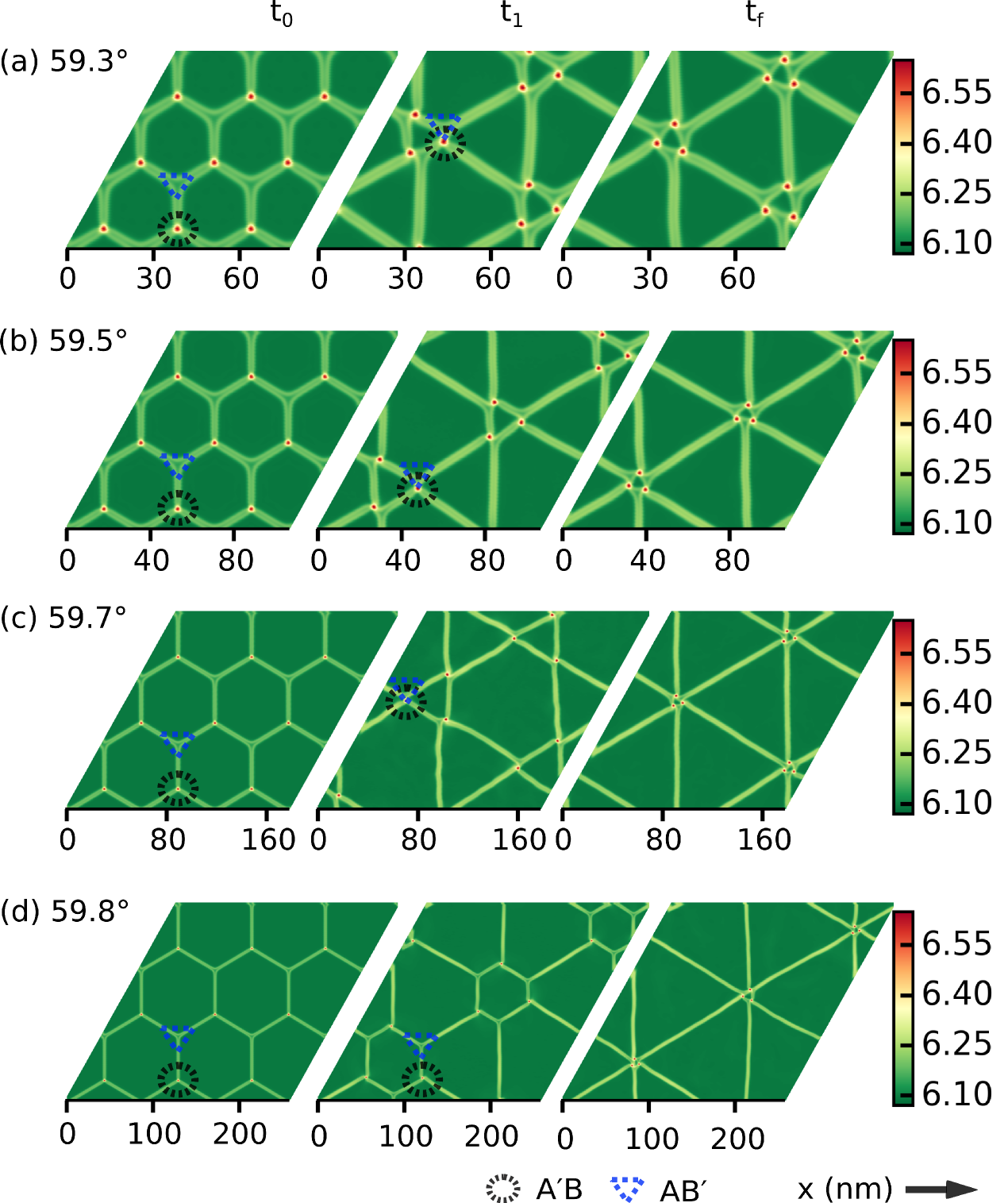
Figure S3: Interlayer separation landscape using the simulated annealing approach during the equilibration of molecular dynamics simulations of a $3\times 3\times 1$ supercell of $\mathrm{tBL\ MoS_{2}}$. $t_{0}$ denotes results with standard relaxation, $t_{1}$ labels results before completely equilibrating, $t_{f}$ denotes results when the trimerization is complete (most stable). Similar results are obtained for other TMDs, as well. The scales of the associated colorbars are for the interlayer separation in Å. Only $\mathrm{A^{\prime}B,\ AB^{\prime}}$ stackings are marked for a few cases.

With $10\times 10\times 1$ moiré supercell

Furthermore, we have also simulated a moiré supercell containing 100 moiré unit cells ($10\times 10\times 1$). This helps us in establishing two important aspects:

(a) The larger number of degrees of freedom can result in complicated lattice reconstructed structures. Some of the transient structures found here resemble the structures observed in recent experiments Weston et al. (2020); Rosenberger et al. (2020). Our results suggest that the distorted hexagons observed in the experiment are results of intrinsic lattice reconstruction. Although, the external substrate, strain etc. can make the transient structures found in our calculations metastable or stable.

(b) Since the $10\times 10\times 1$ supercell contains 100 $\mathrm{A^{\prime}B}$ stackings, a complete trimerization can not be formed (as 100/3 is not an integer). Therefore, complex reconstruction of moiré lattices (other than trimerization) is realized.

We find that the simplest example of lattice reconstruction of moiré lattice is trimerization of the unfavourable stackings. The corresponding figures are shown in the main text (see Fig. 1). However, we find that other complicated lattice reconstructed structures are also possible. It should be noted that the energy difference between the trimerized and other lattice reconstructed structures (such as distorted hexagons, etc.) are only a few tens of meV per moiré lattice. Therefore, the difference between these structures is primarily entropic. To illustrate this, we compute the total energies of the un-reconstructed ($E^{\mathrm{SR}}$), lattice reconstructed structures containing only trimers ($E^{\mathrm{SA}}_{trimer}$), and lattice reconstructed structures containing kagome-like patterns, large parallel domain walls, ($E^{\mathrm{SA}}_{distorted}$) see table 1. It is evident from the table that both the lattice reconstructed structures obtained with SA are significantly energetically lower than the lattice un-reconstructed structures obtained with SR. The difference in energy is $\approx-7$ eV per moiré unit-cell. However, the difference between the energies of the different lattice reconstructed structures is $\approx 50$ meV per moiré unit-cell. For clarity, all the three structures are shown in Fig. S4. We expect that the distorted reconstructed structures such as the one shown in Fig. S4 (c) have higher entropy, and might therefore become the favored structures at finite temperatures via entropic stabilization.

Twist angle	$E^{\mathrm{SR}}$	$E^{\mathrm{SA}}_{trimer}$	$E^{\mathrm{SA}}_{distorted}$
59.5∘	-98699.294 eV	-98706.667 eV	-98706.611 eV

Table 1: Total energies per moiré lattice computed used force-field based simulations. $E^{\mathrm{SR}}$ and $E^{\mathrm{SA}}_{distorted}$ are computed with a moiré supercell containing 100 moiré lattices ($10\times 10\times 1$) and $E^{\mathrm{SA}}_{trimer}$ is computed with a moiré supercell containing 81 moiré lattices ($9\times 9\times 1$).

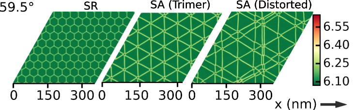
Figure S4: (a): Interlayer separation landscape of $\mathrm{tBLMoS_{2}}$ of lattice un-reconstructed structures, (b): lattice reconstructed structures consisted of only trimers, and (c): lattice reconstructed structures with large parallel domain walls. The scales of the colorbar, in Å and corresponds to interlayer separation.

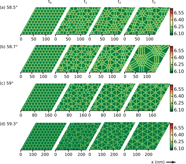
Figure S5: (a) Interlayer separation (ILS) landscape using the simulated annealing approach for several twist angles with $10\times 10\times 1$ moiré supercells. The scales of the associated colorbars are for the interlayer separation in Å. For every twist angle four ILS landscapes are shown, where the snapshots for annealing are taken from 1-1.5 nanosecond molecular dynamics runs. $t_{0}=0$ ns, $t_{1}\sim 0.1-0.2$ ns, $t_{2}\sim 0.3-0.4$ ns, and $t_{3}\sim 1-1.5$ ns i.e. $t_{0}<t_{1}<t_{2}<t_{3}$.

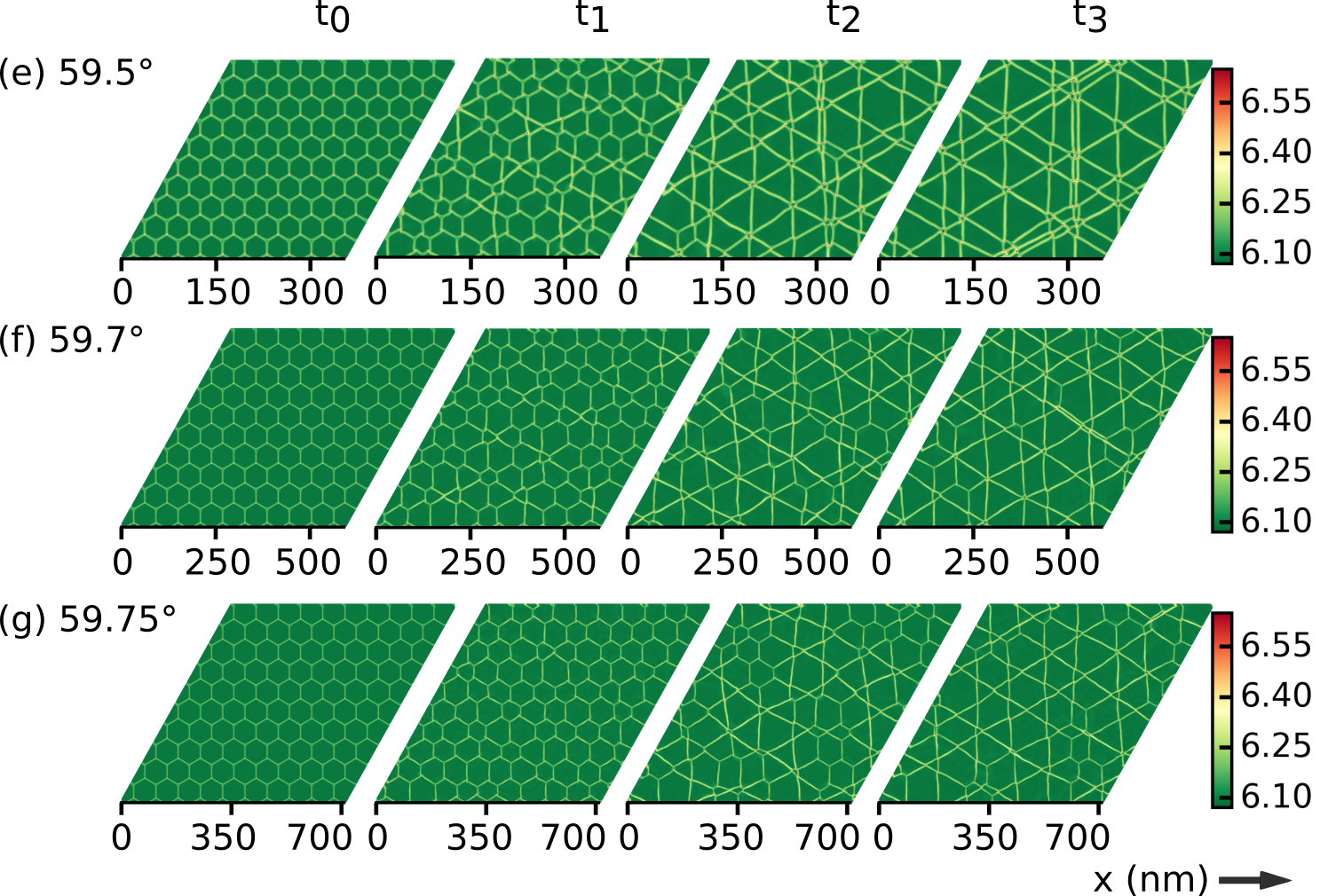
Figure S6: (a) Interlayer separation (ILS) landscape using the simulated annealing approach for several additional twist angles with $10\times 10\times 1$ moiré supercells. The scales of the associated colorbars are for the interlayer separation in Å. For every twist angle four ILS landscapes are shown, where the snapshots for annealing are taken from 1 nanosecond molecular dynamics runs. $t_{0}=0$ ns, $t_{1}\sim 0.3-0.4$ ns, $t_{2}\sim 0.6$ ns and $t_{3}\sim 1$ ns i.e. $t_{0}<t_{1}<t_{2}<t_{3}$.

V V : Confining potential from DFT

To compute the effective moiré potential, we use the following steps:- (a) We average the self-consistent total DFT potential in the out-of-plane direction. (b) We create a map of the local potential using the Voronoi cells obtained from the positions of the Mo atoms ($x_{\mathrm{Mo}},y_{\mathrm{Mo}}$) of bottom layer $\mathrm{MoS_{2}}$ and obtain the macroscopic potential ($V_{\mathrm{M}}(x_{\mathrm{Mo}},y_{\mathrm{Mo}})$). (c) We compute the confining potential by subtracting the average: $V_{\mathrm{conf}}=V_{\mathrm{M}}-\bar{V}_{\mathrm{M}}$. The confining potential is plotted in Fig S7. The electrons (holes) are localized at the $\mathrm{A^{\prime}B}$ ($\mathrm{AA^{\prime}}$) stacking where the confining potential has a minimum (maximum). The minimum and maximum of the potential at these stackings are tabulated in table 2. All these calculations are performed using multi-scale simulations, as outlined above. We also tabulate the first few eigenvalues near VBM and CBM for both un-reconstructed structures (table 3) and lattice reconstructed structures (table 4). As can be seen from the table, the separation between the first few bands near the band edges and associated degeneracies change significantly.

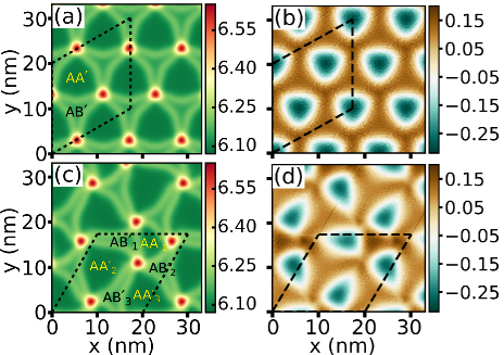
Figure S7: (a), (b): Interlayer separation landscape and the confining moiré potential, respectively, for structures obtained with SR. (c), (d) Interlayer separation landscape and the confining moiré potential, respectively, for structures obtained with SA. The scales of the associated colorbars for the interlayer separation are in Å. The scales of the associated colorbars for moiré potential are in eV. The moiré $\sqrt{3}\times\sqrt{3}\times 1$ cell is marked with black dashed lines. Different stacking locations are marked in (a), (b).

Structure	$V_{\mathrm{AA^{\prime}_{1}}}$ (meV)	$V_{\mathrm{AA^{\prime}_{2}}}$ (meV)	$V_{\mathrm{AA^{\prime}_{3}}}$ (meV)	$V_{\mathrm{AB^{\prime}_{1}}}$ (meV)	$V_{\mathrm{AB^{\prime}_{2}}}$ (meV)	$V_{\mathrm{AB^{\prime}_{3}}}$ (meV)
SR ($\sqrt{3}\times\sqrt{3}\times 1$)	132	132	132	-306	-306	-306
SA ($\sqrt{3}\times\sqrt{3}\times 1$)	171	97	103	-240	-268	-258

Table 2: Moiré potential height at different stackings for the unreconstructed structures obtained with SR and the lattice reconstructed structures obtained with SA.

	$\mathrm{V_{1}}$ (eV)	$\mathrm{V_{2}}$ (eV)	$\mathrm{V_{3}}$ (eV)	$\mathrm{V_{4}}$ (eV)	$\mathrm{C_{1}}$ (eV)	$\mathrm{C_{2}}$ (eV)	$\mathrm{C_{3}}$ (eV)
Structure	[d]	[d]	[d]	[d]	[d]	[d]	[d]
SR ($\sqrt{3}\times\sqrt{3}\times 1$)	-4.342	-4.365	-4.381	-4.395	-3.394	-3.376	-3.337
	[$1\times 3$]	[2$\times$3]	[$1\times 3$]	[$2\times 3$]	[$6\times 3$]	[$2\times 3$]	[$2\times 3$]

Table 3: First few bands near the valence band maximum and the conduction band minimum with the degeneracies specified in brackets.

	$\mathrm{V_{1}}$ (eV)	$\mathrm{V_{2}}$ (eV)	$\mathrm{V_{3}}$ (eV)	$\mathrm{V_{4}}$ (eV)	$\mathrm{C_{1}}$ (eV)	$\mathrm{C_{2}}$ (eV)	$\mathrm{C_{3}}$ (eV)
Structure	[d]	[d]	[d]	[d]	[d]	[d]	[d]
SA ($\sqrt{3}\times\sqrt{3}\times 1$)	-4.32	-4.365	-4.372	-4.379	-3.354	-3.352	-3.348
	[1]	[1]	[2]	[1]	[2]	[3]	[4]

Table 4: First few bands near valence and conduction bands with the degeneracies specified in brackets.

VI VI : Structural relaxation results using DFT

The unit-cell lattice constant of the $\mathrm{BLMoS_{2}}$ is 3.138 Åand the optimum interlayer separation for the most stable $\mathrm{AA^{\prime}}$ stacking is 6.1 Å. Using classical force-field based simulations, we find the reconstruction of the moiré lattices occur for $\theta>58.5^{\circ}$. The characteristic angle of $\theta_{c}\approx 58.5^{\circ}$ is dependent on both the intralayer elastic energy parameters and the stacking energy parameters. Therefore, we expect the characteristic angle for the onset of lattice reconstruction with DFT to be slightly different from that seen in force-field-based simulations. To prove purely using DFT that the reconstructed structures obtained with classical force-field based simulations are more stable than the un-reconstructed structures, one would have to perform several huge DFT calculations. This is, of course, practically impossible as the system contains $2.5\times 10^{4}$ to $10^{6}$ atoms. One possible strategy to circumvent this immensely computationally expensive task is to tune the characteristic angle for the onset of lattice reconstruction and reduce the moiré supercell size on which DFT based relaxations are performed. This can be achieved by applying a small compressive strain.

We have applied a series of small compressive strains and created the moiré lattices of $\mathrm{MoS_{2}}$ for $\theta=58.53^{\circ}$ with systems containing 24966 atoms. We have performed SR and SA on the $\sqrt{3}\times\sqrt{3}\times 1$ supercell of the moiré lattice using force-field based simulations. Using these structures as starting configurations, we have performed structural relaxation using DFT with SIESTA. As can be seen from the table 5, the lattice reconstructed structures obtained with SA becomes more stable than the lattice un-reconstructed structures obtained with SR when the compressive compressive strain exceeds a threshold. Thus, we have established the reconstruction of moiré lattices in twisted TMD bilayers close to $60^{\circ}$ twist angles, using both classical force-field based calculations and first-principles based DFT calculations. We show the change in total energies per moiré unit-cell during the relaxation based on DFT in Fig S8.

$\theta$ (supercell)	Strain	Moiré supercell	$\Delta E$ per moiré
		$\sqrt{3}a_{\mathrm{M}}$
58.47∘ ($\sqrt{3}\times\sqrt{3}\times 1$)	0%	202.42 Å	8.4 eV
58.47∘ ($\sqrt{3}\times\sqrt{3}\times 1$)	-0.7%	201 Å	1.8 eV
58.47∘ ($\sqrt{3}\times\sqrt{3}\times 1$)	-1.5%	199.3 Å	0.03 eV
58.47∘ ($\sqrt{3}\times\sqrt{3}\times 1$)	-2 %	198.03 Å	-0.175 eV

Table 5: $\Delta E=(E^{\mathrm{SA}}-E^{\mathrm{SR}})/3$: Total energy differences between the trimerized structure (SA) and lattice un-reconstructed structure (SR) for several small compressive strains computed after relaxations performed with DFT.

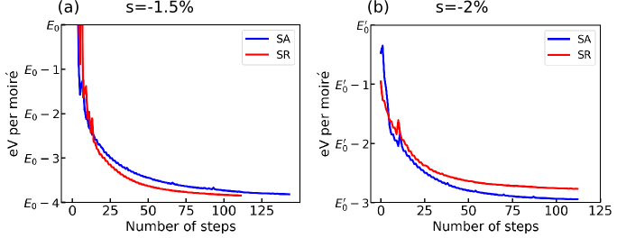
Figure S8: The change in total energies during the relaxation in SIESTA for a compressive strain of $-1.5\%$ (in (a)) and $-2\%$ (in (b)). $E_{0}$ (=-6968752 eV) and $E_{0}^{\prime}$ (=-6968695 eV) are the offsets for the total energy. SR denotes standard relaxation and SA denotes simulated annealing.

We also compute the bi-axial strain dependence of the energetics between structures obtained with SR and SA using force-field based simulations. We find the energy differences between these structures are sensitive to strain (Fig. S9). The lattice reconstructed structures are always more stable than the structures obtained with SR for any biaxial compressive strain. However, under sufficient tensile strain, the structures obtained with SR are more stable than the lattice reconstructed structures. The largest tensile strain applied in our simulation is $\approx 3.8\%$

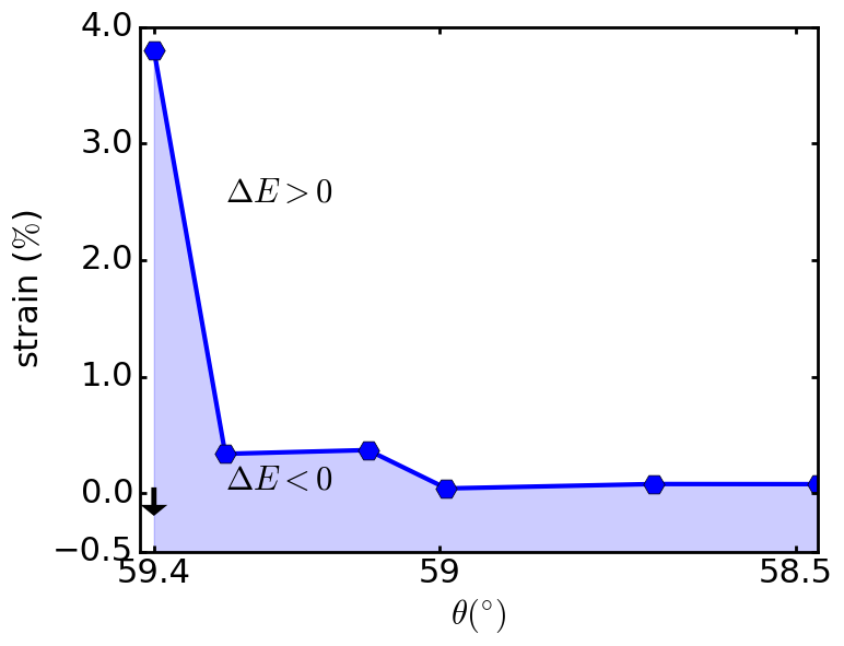
Figure S9: Strain-twist angle phase diagram computed with force-field based simulations. When the energy difference between lattice reconstructed and un-reconstructed structures ($\Delta E$) is negative, the lattice reconstructed structures are more stable (the shaded region). Under the application of large bi-axial tensile strain, the lattice un-reconstructed structures obtained with SR become energetically more stable. All the calculations are performed on a $\sqrt{3}\times\sqrt{3}\times 1$ supercell for several twist angles with classical force-field based simulations.

References

- Bistritzer and MacDonald (2011) R. Bistritzer and A. H. MacDonald, Proceedings of the National Academy of Sciences 108, 12233 (2011).
- Cao et al. (2018a) Y. Cao, V. Fatemi, A. Demir, S. Fang, S. L. Tomarken, J. Y. Luo, J. D. Sanchez-Yamagishi, K. Watanabe, T. Taniguchi, E. Kaxiras, R. C. Ashoori, and P. Jarillo-Herrero, Nature 556, 80 (2018a).
- Cao et al. (2018b) Y. Cao, V. Fatemi, S. Fang, K. Watanabe, T. Taniguchi, E. Kaxiras, and P. Jarillo-Herrero, Nature 556, 43 (2018b).
- Yankowitz et al. (2019) M. Yankowitz, S. Chen, H. Polshyn, Y. Zhang, K. Watanabe, T. Taniguchi, D. Graf, A. F. Young, and C. R. Dean, Science 363, 1059 (2019).
- Naik and Jain (2018) M. H. Naik and M. Jain, Phys. Rev. Lett. 121, 266401 (2018).
- Naik et al. (2019a) M. H. Naik, S. Kundu, I. Maity, and M. Jain, arXiv preprint arXiv:1908.10399 (2019a).
- Fleischmann et al. (2019) M. Fleischmann, R. Gupta, S. Sharma, and S. Shallcross, arXiv preprint arXiv:1901.04679 (2019).
- Wang et al. (2020) L. Wang, E.-M. Shih, A. Ghiotto, L. Xian, D. A. Rhodes, C. Tan, M. Claassen, D. M. Kennes, Y. Bai, B. Kim, K. Watanabe, T. Taniguchi, X. Zhu, J. Hone, A. Rubio, A. N. Pasupathy, and C. R. Dean, Nature Materials (2020), 10.1038/s41563-020-0708-6.
- Zhang et al. (2019) Z. Zhang, Y. Wang, K. Watanabe, T. Taniguchi, K. Ueno, E. Tutuc, and B. J. LeRoy, arXiv preprint arXiv:1910.13068 (2019).
- Wu et al. (2019) F. Wu, T. Lovorn, E. Tutuc, I. Martin, and A. H. MacDonald, Phys. Rev. Lett. 122, 086402 (2019).
- Bi et al. (2019) Z. Bi, N. F. Q. Yuan, and L. Fu, Phys. Rev. B 100, 035448 (2019).
- Angeli and MacDonald (2020) M. Angeli and A. H. MacDonald, arXiv e-prints , arXiv:2008.01735 (2020), arXiv:2008.01735 [cond-mat.str-el] .
- Pan et al. (2020) H. Pan, F. Wu, and S. Das Sarma, Phys. Rev. Research 2, 033087 (2020).
- Zhan et al. (2020) Z. Zhan, Y. Zhang, P. Lv, H. Zhong, G. Yu, F. Guinea, J. A. Silva-Guillén, and S. Yuan, Phys. Rev. B 102, 241106 (2020).
- Zhai and Yao (2020) D. Zhai and W. Yao, Phys. Rev. Materials 4, 094002 (2020).
- Gargiulo and Yazyev (2017) F. Gargiulo and O. V. Yazyev, 2D Materials 5, 015019 (2017).
- Yoo et al. (2019) H. Yoo, R. Engelke, S. Carr, S. Fang, K. Zhang, P. Cazeaux, S. H. Sung, R. Hovden, A. W. Tsen, T. Taniguchi, K. Watanabe, G.-C. Yi, M. Kim, M. Luskin, E. B. Tadmor, E. Kaxiras, and P. Kim, Nature Materials 18, 448 (2019).
- Lucignano et al. (2019) P. Lucignano, D. Alfè, V. Cataudella, D. Ninno, and G. Cantele, Phys. Rev. B 99, 195419 (2019).
- Nam and Koshino (2017) N. N. T. Nam and M. Koshino, Phys. Rev. B 96, 075311 (2017).
- Leconte et al. (2019) N. Leconte, S. Javvaji, J. An, and J. Jung, arXiv preprint arXiv:1910.12805 (2019).
- Halbertal et al. (2021) D. Halbertal, N. R. Finney, S. S. Sunku, A. Kerelsky, C. Rubio-Verdú, S. Shabani, L. Xian, S. Carr, S. Chen, C. Zhang, L. Wang, D. Gonzalez-Acevedo, A. S. McLeod, D. Rhodes, K. Watanabe, T. Taniguchi, E. Kaxiras, C. R. Dean, J. C. Hone, A. N. Pasupathy, D. M. Kennes, A. Rubio, and D. N. Basov, Nature Communications 12, 242 (2021).
- Pickard and Needs (2011) C. J. Pickard and R. J. Needs, Journal of Physics: Condensed Matter 23, 053201 (2011).
- Stillinger (1999) F. H. Stillinger, Phys. Rev. E 59, 48 (1999).
- Kirkpatrick et al. (1983) S. Kirkpatrick, C. D. Gelatt, and M. P. Vecchi, Science 220, 671 (1983).
- Carr et al. (2018) S. Carr, D. Massatt, S. B. Torrisi, P. Cazeaux, M. Luskin, and E. Kaxiras, Phys. Rev. B 98, 224102 (2018).
- Enaldiev et al. (2020) V. V. Enaldiev, V. Zólyomi, C. Yelgel, S. J. Magorrian, and V. I. Fal’ko, Phys. Rev. Lett. 124, 206101 (2020).
- Weston et al. (2020) A. Weston, Y. Zou, V. Enaldiev, A. Summerfield, N. Clark, V. Zólyomi, A. Graham, C. Yelgel, S. Magorrian, M. Zhou, J. Zultak, D. Hopkinson, A. Barinov, T. H. Bointon, A. Kretinin, N. R. Wilson, P. H. Beton, V. I. Fal’ko, S. J. Haigh, and R. Gorbachev, Nature Nanotechnology (2020).
- Rosenberger et al. (2020) M. R. Rosenberger, H.-J. Chuang, M. Phillips, V. P. Oleshko, K. M. McCreary, S. V. Sivaram, C. S. Hellberg, and B. T. Jonker, ACS Nano 14, 4550 (2020).
- (29) See Supplementary Information (SI) at http://------ for simulation details, reconstruction of other TMDs, several transient structures, confining moiré potential computed with DFT, and structural relaxation with DFT .
- Jiang and Zhou (2017) J.-W. Jiang and Y.-P. Zhou, (2017).
- Naik et al. (2019b) M. H. Naik, I. Maity, P. K. Maiti, and M. Jain, The Journal of Physical Chemistry C 123, 9770 (2019b).
- Plimpton (1995) S. Plimpton, Journal of Computational Physics 117, 1 (1995).
- Bitzek et al. (2006) E. Bitzek, P. Koskinen, F. Gähler, M. Moseler, and P. Gumbsch, Phys. Rev. Lett. 97, 170201 (2006).
- Togo and Tanaka (2015) A. Togo and I. Tanaka, Scripta Materialia 108, 1 (2015).
- Kohn and Sham (1965) W. Kohn and L. J. Sham, Phys. Rev. 140, A1133 (1965).
- Lin et al. (2014) L. Lin, A. García, G. Huhs, and C. Yang, Journal of Physics: Condensed Matter 26, 305503 (2014).
- Soler et al. (2002) J. M. Soler, E. Artacho, J. D. Gale, A. García, J. Junquera, P. Ordejón, and D. Sánchez-Portal, Journal of Physics: Condensed Matter 14, 2745 (2002).
- zhe Yu et al. (2018) V. W. zhe Yu, F. Corsetti, A. García, W. P. Huhn, M. Jacquelin, W. Jia, B. Lange, L. Lin, J. Lu, W. Mi, A. Seifitokaldani, Álvaro Vázquez-Mayagoitia, C. Yang, H. Yang, and V. Blum, Computer Physics Communications 222, 267 (2018).
- Lin et al. (2009) L. Lin, J. Lu, L. Ying, R. Car, and W. E, Commun. Math. Sci. 7, 755 (2009).
- Troullier and Martins (1991) N. Troullier and J. L. Martins, Phys. Rev. B 43, 1993 (1991).
- Dion et al. (2004) M. Dion, H. Rydberg, E. Schröder, D. C. Langreth, and B. I. Lundqvist, Phys. Rev. Lett. 92, 246401 (2004).
- Cooper (2010) V. R. Cooper, Phys. Rev. B 81, 161104 (2010).
- van Setten et al. (2018) M. van Setten, M. Giantomassi, E. Bousquet, M. Verstraete, D. Hamann, X. Gonze, and G.-M. Rignanese, Computer Physics Communications 226, 39 (2018).
- Liang et al. (2017) L. Liang, A. A. Puretzky, B. G. Sumpter, and V. Meunier, Nanoscale 9, 15340 (2017).
- Alden et al. (2013) J. S. Alden, A. W. Tsen, P. Y. Huang, R. Hovden, L. Brown, J. Park, D. A. Muller, and P. L. McEuen, Proceedings of the National Academy of Sciences 110, 11256 (2013).
- Modes and Kamien (2013) C. D. Modes and R. D. Kamien, Soft Matter 9, 11078 (2013).
- Maity et al. (2018) I. Maity, P. K. Maiti, and M. Jain, Phys. Rev. B 97, 161406 (2018).
- Zhang and Tadmor (2018) K. Zhang and E. B. Tadmor, Journal of the Mechanics and Physics of Solids 112, 225 (2018).
- Maity et al. (2020) I. Maity, M. H. Naik, P. K. Maiti, H. R. Krishnamurthy, and M. Jain, Phys. Rev. Research 2, 013335 (2020).
- Sun et al. (2012) K. Sun, A. Souslov, X. Mao, and T. C. Lubensky, Proceedings of the National Academy of Sciences 109, 12369 (2012).
- Riste (2012) T. Riste, Ordering in strongly fluctuating condensed matter systems, Vol. 50 (Springer Science & Business Media, 2012).
- Zhang et al. (2018) C. Zhang, M.-Y. Li, J. Tersoff, Y. Han, Y. Su, L.-J. Li, D. A. Muller, and C.-K. Shih, Nature Nanotechnology 13, 152 (2018).
- Xu et al. (2020) Y. Xu, S. Liu, D. A. Rhodes, K. Watanabe, T. Taniguchi, J. Hone, V. Elser, K. F. Mak, and J. Shan, Nature 587, 214 (2020).
- Andersen et al. (2019) T. I. Andersen, G. Scuri, A. Sushko, K. De Greve, J. Sung, Y. Zhou, D. S. Wild, R. J. Gelly, H. Heo, K. Watanabe, T. Taniguchi, P. Kim, H. Park, and M. D. Lukin, arXiv e-prints , arXiv:1912.06955 (2019), arXiv:1912.06955 [cond-mat.mes-hall] .
- Scuri et al. (2020) G. Scuri, T. I. Andersen, Y. Zhou, D. S. Wild, J. Sung, R. J. Gelly, D. Bérubé, H. Heo, L. Shao, A. Y. Joe, A. M. Mier Valdivia, T. Taniguchi, K. Watanabe, M. Lončar, P. Kim, M. D. Lukin, and H. Park, Phys. Rev. Lett. 124, 217403 (2020).
- Baek et al. (2020) H. Baek, M. Brotons-Gisbert, Z. X. Koong, A. Campbell, M. Rambach, K. Watanabe, T. Taniguchi, and B. D. Gerardot, Science Advances 6 (2020), 10.1126/sciadv.aba8526.
- Ni et al. (2019) G. X. Ni, H. Wang, B.-Y. Jiang, L. X. Chen, Y. Du, Z. Y. Sun, M. D. Goldflam, A. J. Frenzel, X. M. Xie, M. M. Fogler, and D. N. Basov, Nature Communications 10, 4360 (2019).
- Jiang et al. (2016) L. Jiang, Z. Shi, B. Zeng, S. Wang, J.-H. Kang, T. Joshi, C. Jin, L. Ju, J. Kim, T. Lyu, Y.-R. Shen, M. Crommie, H.-J. Gao, and F. Wang, Nature Materials 15, 840 (2016).
- Holler et al. (2020) J. Holler, S. Meier, M. Kempf, P. Nagler, K. Watanabe, T. Taniguchi, T. Korn, and C. Schüller, Applied Physics Letters 117, 013104 (2020).
- Gadelha et al. (2020) A. C. Gadelha, D. A. A. Ohlberg, C. Rabelo, E. G. S. Neto, T. L. Vasconcelos, J. L. Campos, J. S. Lemos, V. Ornelas, D. Miranda, R. Nadas, F. C. Santana, K. Watanabe, T. Taniguchi, B. van Troeye, M. Lamparski, V. Meunier, V.-H. Nguyen, D. Paszko, J.-C. Charlier, L. C. Campos, L. G. Cançado, G. Medeiros-Ribeiro, and A. Jorio, arXiv e-prints , arXiv:2006.09482 (2020), arXiv:2006.09482 [cond-mat.mes-hall] .