Nikhef-2019-056

MPP-2019-252

Testing Lepton Flavour Universality with (Semi)-Leptonic $\boldsymbol{D_{(s)}}$ Decays

Robert Fleischer ^a,b, Ruben Jaarsma ^a and Gabriël Koole ^a,c

^aNikhef, Science Park 105, NL-1098 XG Amsterdam, Netherlands

^bFaculty of Science, Vrije Universiteit Amsterdam,
NL-1081 HV Amsterdam, Netherlands

^cMax Planck Institute for Physics,
Föhringer Ring 6, 80805 München, Germany

Data in $B$-meson decays indicate violations of lepton flavour universality, thereby raising the question about such phenomena in the charm sector. We perform a model-independent analysis of NP contributions in (semi)-leptonic decays of $D_{(s)}$ mesons which originate from $c\to d\bar{\ell}\nu_{\ell}$ and $c\to s\bar{\ell}\nu_{\ell}$ charge-current interactions. Starting from the most general low-energy effective Hamiltonian containing four-fermion operators and the corresponding short-distance coefficients, we explore the impact of new (pseudo)-scalar, vector and tensor operators and constrain their effects through the interplay with current data. We pay special attention to the elements $|V_{cd}|$ and $|V_{cs}|$ of the Cabibbo–Kobayashi–Maskawa matrix and extract them from the $D_{(s)}$ decays in the presence of possible NP decay contributions, comparing them with determinations utilizing unitarity. We find a picture in agreement with the Standard Model within the current uncertainties. Using the results from our analysis, we make also predictions for leptonic $D_{(s)}^{+}\to e^{+}\nu_{e}$ modes which could be hugely enhanced with respect to their tiny Standard Model branching ratios. It will be interesting to apply our strategy at the future high-precision frontier.

December 2019

1 Introduction

Forty-five years after the discovery of the charm quark, flavour physics has developed into a broad line of research, allowing us to probe the Standard Model (SM) with unprecedented sensitivity to new interactions and particles at energy scales far beyond the TeV regime which is directly accessible at the Large Hadron Collider (LHC) today [1].

In these explorations, decays of $B$ mesons usually play the key role. Measurements by the BaBar, Belle and LHCb collaborations of processes originating from $b\to c\ell^{-}\bar{\nu}_{\ell}$ and $b\to s\ell^{+}\ell^{-}$ quark-level transitions indicate deviations from the SM, where the following observables are in the focus ($\ell=e,\mu$):

$$\mathcal{R}_{D^{(*)}}\equiv\frac{\mathcal{B}(B\to D^{(*)}\tau^{-}\nu_{\tau})}{\mathcal{B}(B\to D^{(*)}\ell^{-}\nu_{\ell})},\hskip 28.45274ptR_{K^{(*)}}\equiv\frac{\mathcal{B}(B\to K^{(*)}\mu^{+}\mu^{-})}{\mathcal{B}(B\to K^{(*)}e^{+}e^{-})}.$$ (1)

The experimental values of these ratios show tensions with respect to the corresponding SM predictions at the $(2\mbox{--}3)\sigma$ level (for recent reviews, see, e.g., Refs. [2, 3]). In particular, the data raise the exciting question of a possible violation of a central feature of the SM: lepton flavour universality (LFU).

On the theory side, various models of New Physics (NP), i.e. physics lying beyond the SM, have been proposed that could explain the $B$-decay anomalies, allowing in particular also for violations of LFU. Important specific scenarios are given by leptoquark models [7, 8, 9, 10, 11, 12], $Z^{\prime}$ models [13, 14, 15] or Two-Higgs-Doublet models [16, 17, 18], implying usually a rich phenomenology of patterns and correlations among various observables.

In view of the potential violation of LFU in $B$-meson decays, it is interesting to search for such phenomena and possible signals of physics beyond the SM also in the charm sector. In fact, in NP scenarios allowing us to describe the $B$ decay anomalies, effects may also arise in weak decay processes of $D$ mesons. In Ref. [19], rare decays of the kind $D\to\pi\ell\ell$ and $D_{s}\to K\ell\ell$ have recently been analyzed. These modes arise form flavour-changing neutral current (FCNC) interactions and are the counterparts of the rare $B$ decays entering the $R_{K^{(*)}}$ ratios in Eq. (1). Such processes are usually considered as particularly powerful NP probes as they are not allowed in the SM at the tree level but originate from quantum fluctuations at the loop level. For an analysis of rare $s\to d$ kaon processes, see Ref. [20]. However, decays caused by charged-current interactions at the SM tree level may also be affected by NP effects, as indicated by the $\mathcal{R}_{D^{(*)}}$ observables in Eq. (1). This opens up the door to investigate such NP effects in the corresponding decays of charmed mesons as well [21].

In this paper, we shall probe LFU violating effects through (semi)-leptonic $D_{(s)}$-meson decays, applying the strategy proposed in Refs. [22, 23] for (semi)-leptonic decays of $B_{(s)}$ mesons. Precise lattice QCD calculations and experimental information on leptonic and semileptonic decays of $D_{(s)}$ mesons, arising from $c\to d\bar{\ell}\nu_{\ell}$ or $c\to s\bar{\ell}\nu_{\ell}$ quark-level transitions, allow us to test LFU in the charm sector. In particular, we constrain short-distance coefficients describing physics beyond the SM through a comparison of theoretical calculations with experimental data. Furthermore, we will extract the Cabibbo–Kobayashi–Maskawa (CKM) matrix elements $|V_{cd}|$ and $|V_{cs}|$ from weak charm decays, also in the presence of NP contributions, and will make predictions for leptonic $D_{(s)}^{+}\to e^{+}\nu_{e}$ decays. These modes could be hugely enhanced through new pseudoscalar contributions, in fact close to the current experimental upper bounds on the corresponding branching ratios.

The outline of this paper is as follows: in Section 2, we introduce the most general basis of local operators describing (semi)-leptonic $D_{(s)}$ decays, and discuss the resulting low-energy effective Hamiltonian. Furthermore, we exploit the unitarity of the CKM matrix to determine $|V_{cd(s)}|$ without any use of information following from $D_{(s)}$ decay data. In Section 3, we utilize current experimental information on leptonic $D_{(s)}$ decays to constrain the short-distance coefficients for NP contributions. Subsequently, in Section 4 we perform a similar analysis for semileptonic $D_{(s)}$ decays. In Section 5, we use some of the obtained constraints to determine $|V_{cd}|$ and $|V_{cs}|$ in the presence of pseudoscalar NP interactions. In Section 6, we discuss predictions for leptonic $D_{(s)}^{+}\to e^{+}\nu_{e}$ decays. Finally, we present our conclusions and outlook in Section 7.

2 Theoretical Framework

2.1 Low-Energy Effective Hamiltonian

The charged-current interaction processes underlying weak decays of $D_{(s)}$ mesons can be described by local four-fermion operators with their associated short-distance Wilson coefficient functions. Considering all possible Lorentz structures for decays originating from $c\rightarrow d\bar{\ell}\nu_{\ell}$ or $c\rightarrow s\bar{\ell}\nu_{\ell}$ transitions (with $\ell=e,\mu,\tau$) and assuming neutrinos to be left-handed, we obtain the following operator basis (with $q=d,s$) [24, 25]:

$$\mathcal{O}^{\ell}_{V_{L}} =(\bar{q}_{L}\gamma_{\mu}c_{L})(\bar{\nu}_{\ell L}\gamma^{\mu}\ell_{L}),\hskip 28.45274pt \mathcal{O}^{\ell}_{V_{R}} =(\bar{q}_{R}\gamma_{\mu}c_{R})(\bar{\nu}_{\ell L}\gamma^{\mu}\ell_{L}),$$ (2)

$$\mathcal{O}^{\ell}_{S_{1}} =(\bar{q}_{L}c_{R})(\bar{\nu}_{\ell L}\ell_{R}), \mathcal{O}^{\ell}_{S_{2}} =(\bar{q}_{R}c_{L})(\bar{\nu}_{\ell L}\ell_{R}),$$

$$\mathcal{O}^{\ell}_{T} =(\bar{q}_{L}\sigma^{\mu\nu}c_{R})(\bar{\nu}_{\ell L}\sigma_{\mu\nu}\ell_{R}).$$

The antisymmetric tensor is defined as $\sigma^{\mu\nu}\equiv\frac{i}{2}[\gamma^{\mu},\gamma^{\nu}]$. Using the appropriate Fierz identity, one can show that the tensor operator with opposite quark chiralities vanishes. In our analysis, it will be convenient to switch to an operator basis that contains a single operator describing the scalar interactions and, similarly, a single pseudoscalar operator. To this end, we define the scalar and pseudoscalar operators in the following way:

$$\mathcal{O}^{\ell}_{S}\equiv\frac{1}{2}\big{(}\mathcal{O}^{\ell}_{S_{1}}+\mathcal{O}^{\ell}_{S_{2}}\big{)}=\frac{1}{2}(\bar{q}c)(\bar{\nu}_{\ell L}\ell_{R}),\hskip 22.76219pt \mathcal{O}^{\ell}_{P}\equiv\frac{1}{2}\big{(}\mathcal{O}^{\ell}_{S_{1}}-\mathcal{O}^{\ell}_{S_{2}}\big{)}=\frac{1}{2}(\bar{q}\gamma_{5}c)(\bar{\nu}_{\ell L}\ell_{R}).$$ (3)

The most general effective Hamiltonian containing all possible local operators of the lowest dimension for $c\rightarrow q\bar{\ell}\nu_{\ell}$ transitions can therefore be written as

$$\mathcal{H}_{\text{eff}}=\frac{4G_{F}}{\sqrt{2}}V_{cq}\Big{[}(1+C^{\ell}_{V_{L}})\mathcal{O}^{\ell}_{V_{L}}+C^{\ell}_{V_{R}}\mathcal{O}^{\ell}_{V_{R}}+C^{\ell}_{S}\mathcal{O}^{\ell}_{S}+C^{\ell}_{P}\mathcal{O}^{\ell}_{P}+C^{\ell}_{T}\mathcal{O}^{\ell}_{T}\Big{]},$$ (4)

where the subscripts $V_{L}$, $V_{R}$, $S$, $P$ and $T$ denote the left-handed vector, right-handed vector, scalar, pseudoscalar and tensor contributions, respectively. In the SM, only the left-handed vector operator is present with an overall Wilson coefficient equal to one. In our analysis, we shall assume real Wilson coefficients for simplicity, i.e. that the NP effects do not involve new sources of CP violation. For a discussion of such effects in the analogous $B$ decays, we refer the reader to Ref. [22, 23].

2.2 $|V_{cd}|$ and $|V_{cs}|$ from Unitarity

The CKM matrix elements $V_{cd}$ and $V_{cs}$ are usually determined directly from leptonic and semileptonic $D_{(s)}$ decays and assuming the SM (such an extraction from experimental $D$ decay rates using lattice QCD form factors was performed in Ref. [26]). In this work, we are investigating these decays in the presence of NP contributions, hence we need an independent determination of $V_{cd}$ and $V_{cs}$. To this end, we adopt the Wolfenstein parametrization [27] of the CKM matrix, exploiting its unitarity. Here, $V_{cd}$ and $V_{cs}$ are related to the Wolfenstein parameters $\{\lambda,A,\rho,\eta\}$. Including corrections up to $\mathcal{O}(\lambda^{5})$ yields the following expressions [28, 29]:

$$V_{cd}=-\lambda+\frac{1}{2}A^{2}\lambda^{5}[1-2(\rho+i\eta)]+\mathcal{O}(\lambda^{7}),$$ (5)

$$V_{cs}=1-\frac{1}{2}\lambda^{2}-\frac{1}{8}\lambda^{4}(1+4A^{2})+\mathcal{O}(\lambda^{6}).$$ (6)

The Wolfenstein parameters entering here can be determined without any information from $D_{(s)}$ decays, which is a very advantageous feature of the charm system. The parameters $\lambda$ and $A$ are related to the CKM elements $V_{us}$ and $V_{cb}$, respectively. The absolute value of $V_{us}$ is determined from the experimental information on kaon decays and assuming the SM. The current average of the results from semileptonic $K^{0}_{S}$, $K^{0}_{L}$ and $K^{\pm}$ decays, combined with $K\to\mu\nu(\gamma)$ decays, is given as follows [30]:

$$|V_{us}|=0.2243\pm 0.0005,$$ (7)

where the SM has been assumed. For $|V_{cb}|$, the current world average from exclusive and inclusive semileptonic decays of $B$ mesons to charm takes the following value [30]:

$$|V_{cb}|=A\lambda^{2}+{\cal O}(\lambda^{8})=(42.2\pm 0.8)\times 10^{-3};$$ (8)

measurements of $|V_{cb}|$ obtained from $\mathcal{B}(B\to D^{(*)}\tau\bar{\nu})$ are not included. To determine the remaining Wolfenstein parameters, we further exploit the unitarity of the CKM matrix. The side $R_{b}$ of the unitarity triangle (UT) of the CKM matrix together with the UT angle $\gamma$ allows us to determine $\rho$ and $\eta$. For the determination of $R_{b}$, we use the following current world average for $|V_{ub}|$ obtained from inclusive and exclusive semileptonic $B$ decays assuming the SM [30]:

$$|V_{ub}|=(3.94\pm 0.36)\times 10^{-3},$$ (9)

combined with the result in Eq. (8). There exist tensions at the 3 $\sigma$ level between the inclusive and exclusive determinations of $|V_{cb}|$ and $|V_{ub}|$[31]. However, for our analysis, it has an essentially negligible impact as these CKM parameters enter only through strongly suppressed higher-order corrections: $|V_{ub}|$ appears only in the corrections in Eq. (5), which differ from the leading term by four orders of $\lambda$. The angle $\gamma$ is usually determined from the tree-dominated $B\to DK$ decays which yield $\gamma=(73.5^{+4.2}_{-5.1})^{\circ}$ [30]. However, as possible NP could slightly affect its value, we allow $\gamma$ to be within $[60^{\circ},80^{\circ}]$. Varying $\gamma$ within this range has a very minor impact. Finally, we obtain the following values for $|V_{cd}|$ and $|V_{cs}|$ from the unitarity of the CKM matrix:

$$|V_{cd}|=0.2242\pm 0.0005,$$ (10)

$$|V_{cs}|=0.9736\pm 0.0001.$$ (11)

The important feature of these results is that they are independent of possible NP contributions to (semi)-leptonic charged-current charm transitions, which are usually exploited to determine these CKM matrix elements from experimental data. We shall use them as reference values for our analysis discussed below.

3 Leptonic Decays

Leptonic $D^{+}_{(s)}\rightarrow\ell^{+}\nu_{\ell}$ decays are the simplest and cleanest weak decay class of charmed mesons. All the hadronic dynamics is captured by a single parameter: the $D_{(s)}$-meson decay constant $f_{D^{+}_{(s)}}$. Leptonic decays of $D$ and $D_{s}$ mesons contain the flavour-changing quark transitions $c\rightarrow d$ and $c\rightarrow s$, respectively. Accurate non-perturbative calculations of the decay constants combined with precise experimental results provide excellent opportunities to perform tests of lepton flavour universality.

In the SM, the branching fraction for leptonic $D^{+}_{(s)}$ decays is given as

$$\mathcal{B}(D^{+}_{(s)}\rightarrow\ell^{+}\nu_{\ell})\big{|}_{\text{SM}}=\frac{G_{F}^{2}}{8\pi}|V_{cq}|^{2}f_{D^{+}_{(s)}}^{2}M_{D^{+}_{(s)}}m^{2}_{\ell}\Big{(}1-\frac{m^{2}_{\ell}}{M^{2}_{D^{+}_{(s)}}}\Big{)}^{2}\tau_{D^{+}_{(s)}},$$ (12)

where $G_{F}$ is Fermi’s constant, $\tau_{D^{+}_{(s)}}$ is the lifetime of the $D_{(s)}^{+}$ meson, and $M^{+}_{D_{(s)}}$ and $m_{\ell}$ are the masses of the $D^{+}_{(s)}$ meson and the lepton ($\ell=e,\mu,\tau$), respectively. The decay constants $f_{D^{+}}$ and $f_{D^{+}_{s}}$ are determined from lattice QCD calculations. For our analysis, we use the values determined by the FLAG working group [32]:

$$f_{D^{+}}=(209.0\pm 2.4)\text{ MeV},$$ (13)

$$f_{D^{+}_{s}}=(248.0\pm 1.6)\text{ MeV}.$$ (14)

The resulting leptonic branching fractions in the SM and their experimental values are given in Table 1. Here, we use the values for $|V_{cd}|$ and $|V_{cs}|$ obtained from unitarity, given in Eqs. (10) and (11), respectively. For the $D_{(s)}\to e^{+}\nu_{e}$ decays, only experimental upper bounds are available. This is due to the extremely strong helicity suppression in these processes, which is reflected by the proportionality of the branching fraction to $m_{\ell}^{2}$. However, potential contributions from pseudoscalar NP interactions could lift the helicity suppression in these decays, thereby making them excellent probes for NP. For previous studies of NP effects in these decays, see Refs. [33, 34, 35].

Decay	SM	Experiment
$\mathcal{B}(D^{+}\rightarrow e^{+}\nu_{e})$	$(9.16\pm 0.22)\times 10^{-9}$	$<8.8\times 10^{-6}$	[30]
$\mathcal{B}(D^{+}\rightarrow\mu^{+}\nu_{\mu})$	$(3.89\pm 0.09)\times 10^{-4}$	$(3.74\pm 0.17)\times 10^{-4}$	[30]
$\mathcal{B}(D^{+}\rightarrow\tau^{+}\nu_{\tau})$	$(1.04\pm 0.03)\times 10^{-3}$	$(1.20\pm 0.27)\times 10^{-3}$	[36]
$\mathcal{B}(D_{s}^{+}\rightarrow e^{+}\nu_{e})$	$(1.24\pm 0.02)\times 10^{-7}$	$<8.3\times 10^{-5}$	[30]
$\mathcal{B}(D_{s}^{+}\rightarrow\mu^{+}\nu_{\mu})$	$(5.28\pm 0.08)\times 10^{-3}$	$(5.50\pm 0.23)\times 10^{-3}$	[30]
$\mathcal{B}(D_{s}^{+}\rightarrow\tau^{+}\nu_{\tau})$	$(5.15\pm 0.08)\times 10^{-2}$	$(5.48\pm 0.23)\times 10^{-2}$	[30]

Table 1: Branching ratios of leptonic $D_{s}^{+}$ decays calculated in the SM and comparison with the currently available experimental values.

3.1 Constraints on Pseudoscalar Coefficients

As the scalar contributions coming from $\mathcal{O}_{S}$ vanish due to parity conservation, we start our NP analysis by considering contributions from new pseudoscalar particles. Using the low-energy effective Hamiltonian in Eq. (4), we complement the SM branching fraction with a pseudoscalar contribution and obtain the following expression:

$$\mathcal{B}(D_{(s)}^{+}\rightarrow\ell^{+}\nu_{\ell})=\mathcal{B}(D_{(s)}^{+}\rightarrow\ell^{+}\nu_{\ell})\big{|}_{\text{SM}}\Bigg{|}1+C^{\ell}_{P}\frac{M^{2}_{D^{+}_{(s)}}}{m_{\ell}(m_{c}+m_{q})}\Bigg{|}^{2},$$ (15)

where $C^{\ell}_{P}$ is the short-distance coefficient for the pseudoscalar NP contribution, and $m_{c}$ and $m_{q}$ are the masses of the charm and down (strange) quarks. In these branching fractions, the decay constants are the source of the largest theoretical uncertainties. Moreover, they contain the CKM elements $|V_{cd}|$ or $|V_{cs}|$, which we would finally like to determine from these decays, also in the presence of NP contributions. With this in mind, we consider the following ratio of two leptonic decays:

$$R^{\ell_{1}}_{\ell_{2}}\equiv\frac{\mathcal{B}(D_{(s)}^{+}\rightarrow\ell_{1}^{+}\nu_{\ell_{1}})}{\mathcal{B}(D_{(s)}^{+}\rightarrow\ell_{2}^{+}\nu_{\ell_{2}})}=\frac{\alpha^{\ell_{1}}\big{|}1+\beta^{\ell_{1}}C^{\ell_{1}}_{P}\big{|}^{2}}{\alpha^{\ell_{2}}\big{|}1+\beta^{\ell_{2}}C^{\ell_{2}}_{P}\big{|}^{2}},$$ (16)

where

$$\alpha^{\ell_{1(2)}}=m^{2}_{\ell_{1(2)}}\Big{(}1-\frac{m^{2}_{\ell_{1(2)}}}{M^{2}_{D^{+}_{(s)}}}\Big{)}^{2}\quad\mbox{and}\quad\beta^{\ell_{1(2)}}=\frac{M^{2}_{D^{+}_{(s)}}}{[m_{\ell_{1(2)}}(m_{c}+m_{q})]}.$$ (17)

This observable is theoretically clean as the decay constants and also the CKM matrix elements cancel.

Let us first consider leptonic decays of $D$ mesons. Using the experimental information in Table 1, we obtain the following value for the ratio between two leptonic $D$ decays with tau leptons and muons in the final state:

$$(R^{\tau}_{\mu})^{D}=3.21\pm 0.73,$$ (18)

where we have utilized the recent first observation of the decay $D^{+}\to\tau^{+}\nu_{\tau}$ by the BESIII collaboration [36]. By comparing the experimental value with the corresponding theoretical expression, we determine the allowed regions in the $C^{\mu}_{P}$–$C^{\tau}_{P}$ plane. The result is presented in Fig. 1 (left), where the uncertainties coming from the masses are neglected due to their smallness. The SM prediction ($C^{\mu}_{P}=C^{\tau}_{P}=0$), indicated by the black star, is in agreement with the obtained constraints at the 1$\sigma$ level.

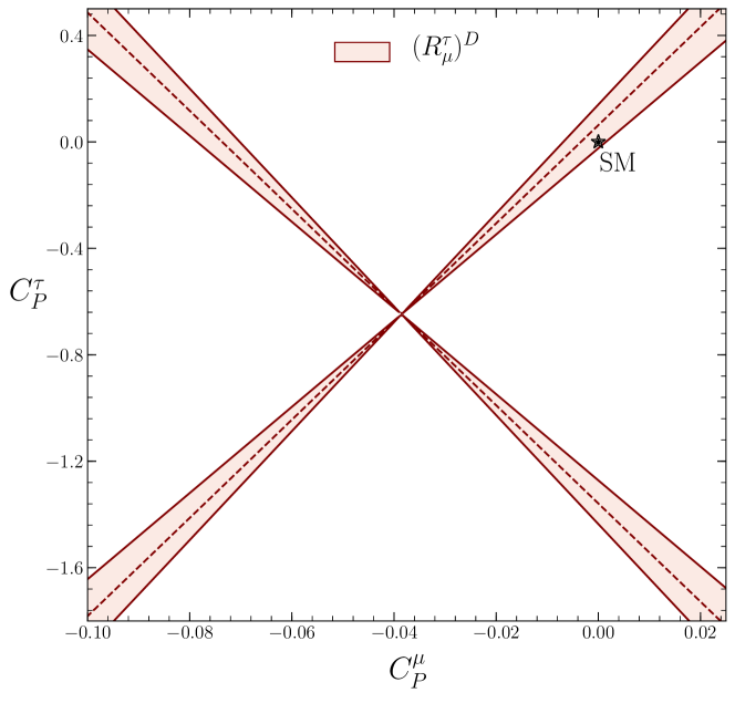
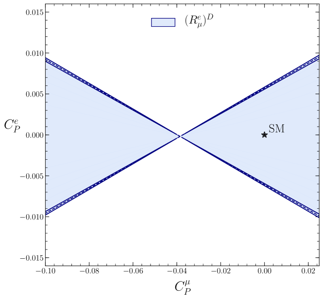
Figure 1: The allowed regions in the $C^{\mu}_{P}$–$C^{\tau}_{P}$ (left) and $C^{\mu}_{P}$–$C^{e}_{P}$ (right) planes following from the ratios $(R^{\tau}_{\mu})^{D}$ and $(R^{e}_{\mu})^{D}$, respectively. The black stars indicate the SM predictions.

For electrons and muons in the final state, we obtain

$$(R^{e}_{\mu})^{D}<(2.35\pm 0.11)\times 10^{-2}.$$ (19)

Comparison with the corresponding theoretical expression allows us to calculate the allowed regions in the $C^{\mu}_{P}$–$C^{e}_{P}$ plane. For the branching fraction $\mathcal{B}(D^{+}\to e^{+}\nu_{e})$, only an experimental upper bound is available, resulting in the large wedge-shaped allowed regions in the panel on the right-hand side of Fig. 1. The SM prediction ($C^{\mu}_{P}=C^{e}_{P}=0$) lies within the obtained 1 $\sigma$ contour. A future measurement of $\mathcal{B}(D^{+}\to e^{+}\nu_{e})$ would allow us to determine more stringent constraints in the $C^{\mu}_{P}$–$C^{e}_{P}$ plane from the $(R^{e}_{\mu})^{D}$ ratio, in analogy to the constraints following from $(R^{\tau}_{\mu})^{D}$.

For $D_{s}$ decays, we perform a similar analysis in the presence of pseudoscalar NP. From the experimental information on leptonic $D_{s}$ decays in Table 1, we obtain the following value for $(R^{\tau}_{\mu})^{D_{s}}$:

$$(R^{\tau}_{\mu})^{D_{s}}=9.96\pm 0.59.$$ (20)

Using this result, we constrain the corresponding short-distance coefficients. The resulting allowed regions in the $C^{\mu}_{P}$–$C^{\tau}_{P}$ plane are shown in the panel on the left-hand side in Fig. 2. For $(R^{e}_{\mu})^{D_{s}}$, we obtain the experimental value

$$(R^{e}_{\mu})^{D_{s}}<(1.51\pm 0.06)\times 10^{-2}.$$ (21)

By comparing our theoretical expression with the experimental information, we obtain the allowed regions in the $C^{\mu}_{P}$–$C^{e}_{P}$ plane shown in the panel on the right-hand side of Fig. 2. We observe that the obtained 1$\sigma$ contours for both $(R^{\tau}_{\mu})^{D_{s}}$ and $(R^{e}_{\mu})^{D_{s}}$ contain the SM predictions. We would like to note that also for $\mathcal{B}(D^{+}_{s}\to e^{+}\nu_{e})$, only an experimental upper bound is available. A future measurement of this branching fraction would allow us to put more stringent constraints on the relevant NP coefficients. We shall return to $D^{+}_{(s)}\to e^{+}\nu_{e}$ decays in Section 6.

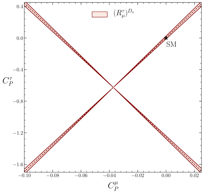
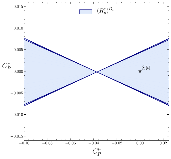
Figure 2: The allowed regions in the $C^{\mu}_{P}$–$C^{\tau}_{P}$ (left) and $C^{\mu}_{P}$–$C^{e}_{P}$ (right) planes following from the ratios $(R^{\tau}_{\mu})^{D_{s}}$ and $(R^{e}_{\mu})^{D_{s}}$, respectively. The black stars indicate the SM predictions.

3.2 Constraints on Vector Coefficients

Besides pseudoscalar NP contributions, the SM branching fraction may also be complemented by contributions from additional vector interactions. Including possible left-handed (LH) vector interactions leads to the following branching fraction:

$$\mathcal{B}(D_{(s)}^{+}\rightarrow\ell^{+}\nu_{\ell})=\mathcal{B}(D_{(s)}^{+}\rightarrow\ell^{+}\nu_{\ell})\big{|}_{\text{SM}}\Big{|}1+C^{\ell}_{V_{L}}\Big{|}^{2},$$ (22)

where $C^{\ell}_{V_{L}}$ is the short-distance coefficient for the LH vector interaction. Just as for the pseudoscalar coefficients, we need a theoretically clean observable for the extraction of constraints on the vector coefficients. In analogy to Eq. (16), we define the ratio of two leptonic branching fractions with different leptons in the final state:

$$R^{\ell_{1}}_{\ell_{2}}\equiv\frac{\mathcal{B}(D_{(s)}^{+}\rightarrow\ell_{1}^{+}\nu_{\ell_{1}})}{\mathcal{B}(D_{(s)}^{+}\rightarrow\ell_{2}^{+}\nu_{\ell_{2}})}=\frac{\alpha^{\ell_{1}}\big{|}1+C^{\ell_{1}}_{V_{L}}\big{|}^{2}}{\alpha^{\ell_{2}}\big{|}1+C^{\ell_{2}}_{V_{L}}\big{|}^{2}}.$$ (23)

We constrain the LH vector coefficients by comparing the theoretical expressions to the experimental information in Eqs. (18–21). The obtained allowed regions in the $C^{\mu}_{V_{L}}$–$C^{\tau}_{V_{L}}$ and $C^{\mu}_{V_{L}}$–$C^{e}_{V_{L}}$ planes are given in Fig. 3.

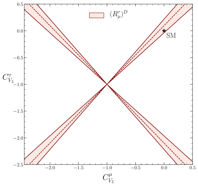
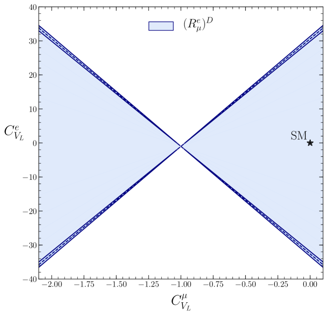
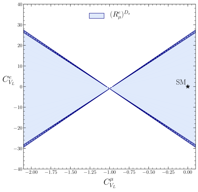
Figure 3: Allowed regions in the $C^{\mu}_{V_{L}}$–$C^{\tau}_{V_{L}}$ plane using the ratios $(R^{\tau}_{\mu})^{D}$ (top left) and $(R^{\tau}_{\mu})^{D_{s}}$ (bottom left), and in the $C^{\mu}_{V_{L}}$–$C^{e}_{V_{L}}$ plane using the ratios $(R^{e}_{\mu})^{D}$ (top right) and $(R^{e}_{\mu})^{D_{s}}$ (bottom right). The black stars indicate the SM predictions.

We proceed our analysis by considering right-handed (RH) vector NP interactions. The branching fraction including RH vector contributions takes the following form:

$$\mathcal{B}(D_{(s)}^{+}\rightarrow\ell^{+}\nu_{\ell})=\mathcal{B}(D_{(s)}^{+}\rightarrow\ell^{+}\nu_{\ell})\big{|}_{\text{SM}}\Big{|}1-C^{\ell}_{V_{R}}\Big{|}^{2},$$ (24)

where $C^{\ell}_{V_{R}}$ is the short-distance coefficient for the RH vector interaction.

Just as for the LH vector coefficients, we define the ratio of two leptonic branching fractions with different leptons in the final state:

$$R^{\ell_{1}}_{\ell_{2}}\equiv\frac{\mathcal{B}(D_{(s)}^{+}\rightarrow\ell_{1}^{+}\nu_{\ell_{1}})}{\mathcal{B}(D_{(s)}^{+}\rightarrow\ell_{2}^{+}\nu_{\ell_{2}})}=\frac{\alpha^{\ell_{1}}\big{|}1-C^{\ell_{1}}_{V_{R}}\big{|}^{2}}{\alpha^{\ell_{2}}\big{|}1-C^{\ell_{2}}_{V_{R}}\big{|}^{2}}.$$ (25)

Using the experimental constraints, we obtain the allowed regions in the $C^{\mu}_{V_{R}}$–$C^{\tau}_{V_{R}}$ and $C^{\mu}_{V_{R}}$–$C^{e}_{V_{R}}$ planes shown in Fig. 4.

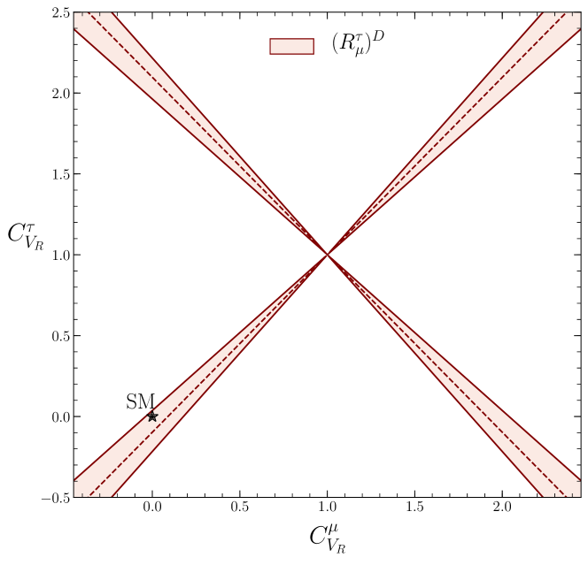
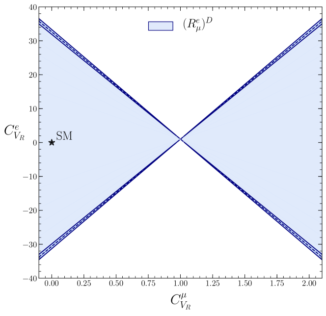
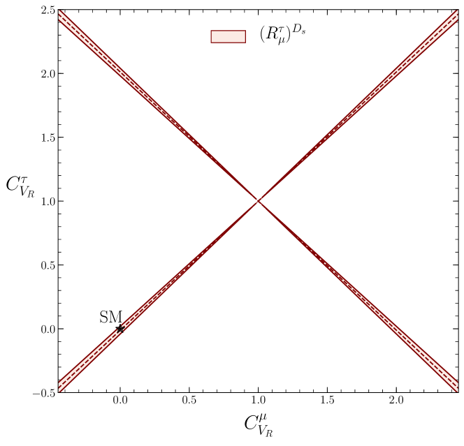
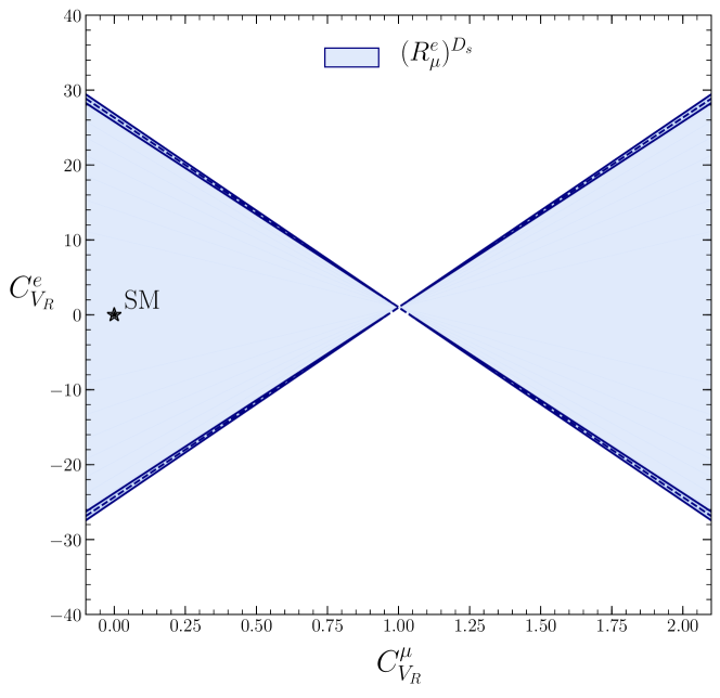
Figure 4: Allowed regions in the $C^{\mu}_{V_{R}}$–$C^{\tau}_{V_{R}}$ plane using the ratios $(R^{\tau}_{\mu})^{D}$ (top left) and $(R^{\tau}_{\mu})^{D_{s}}$ (bottom left), and in the $C^{\mu}_{V_{R}}$–$C^{e}_{V_{R}}$ plane using the ratios $(R^{e}_{\mu})^{D}$ (top right) and $(R^{e}_{\mu})^{D_{s}}$ (bottom right). The black stars indicate the SM predictions.

4 Semileptonic Decays

Semileptonic $D_{(s)}$ decays provide further powerful ways to constrain the short-distance NP coefficients. Since they are driven by the same $c\to d\bar{\ell}\nu_{\ell}$ and $c\to s\bar{\ell}\nu_{\ell}$ quark transitions, these processes are effectively described by the same local operators. Consequently, constraints on the short-distance coefficients coming from semileptonic decays can be utilized to complement those from leptonic decays.

4.1 $D\to P\bar{\ell}\nu_{\ell}$ Decays

First, we consider the semileptonic $D$ decays of the form $D\to P\bar{\ell}\nu_{\ell}$, where $P$ denotes a pseudoscalar meson. The differential branching fraction is given in the SM as follows [25]:

$$\begin{split}\frac{d\mathcal{B}(D\rightarrow P\bar{\ell}\nu_{\ell})}{dq^{2}}\Bigg{|}_{\text{SM}}&=\frac{G_{F}^{2}\tau_{D}|V_{cq}|^{2}}{24\pi^{3}M_{D}^{2}}\Bigg{[}\frac{(H^{P}_{V,0})^{2}}{4}\Big{(}1+\frac{m_{\ell}^{2}}{2q^{2}}\Big{)}+\frac{3}{8}\frac{m_{\ell}^{2}}{q^{2}}(H^{P}_{V,s})^{2}\Bigg{]}\frac{(q^{2}-m_{\ell}^{2})^{2}}{q^{2}}|\vec{p}_{P}|,\end{split}$$ (26)

where $q^{2}$ is the four-momentum of the lepton-neutrino pair, satisfying the relation

$$m_{\ell}^{2}\leq q^{2}\leq(M_{D}-M_{P})^{2}.$$ (27)

In order to calculate the amplitudes $H^{P}_{V,0}$ and $H^{P}_{V,s}$, hadronic form factors are needed, requiring non-perturbative methods. In the literature, various form-factor parametrizations were proposed (for a more detailed discussion, see Appendix A). In Table 2, the SM branching fractions for semileptonic $D\to\pi$ and $D\to K$ decays with electrons or muons in the final states are given, along with their experimental counterparts. For the SM predictions, we used the values of $|V_{cd}|$ and $|V_{cs}|$ in Eqs. (10) and (11), respectively, obtained from the unitarity of the CKM matrix. Furthermore, we applied the lattice results given in Refs.  [37] and [38], adopting double-pole and $z$-series parametrizations, respectively. As the latter approach results in smaller uncertainties for the branching fractions, we will use it in our analysis outlined below. For a studies using quark model caclulations, we refer the reader to Refs. [39, 40].

Decay	Double-pole	$z$-series	Experiment
$\mathcal{B}(D^{0}\rightarrow\pi^{-}e^{+}\nu_{e})$	$(3.21\pm 0.68)\times 10^{-3}$	$(2.64\pm 0.31)\times 10^{-3}$	$(2.91\pm 0.04)\times 10^{-3}$
$\mathcal{B}(D^{0}\rightarrow K^{-}e^{+}\nu_{e})$	$(3.64\pm 0.76)\times 10^{-2}$	$(3.49\pm 0.29)\times 10^{-2}$	$(3.542\pm 0.035)\times 10^{-2}\hskip 1.70717pt$
$\mathcal{B}(D^{+}\rightarrow\pi^{0}e^{+}\nu_{e})$	$(4.17\pm 0.88)\times 10^{-3}$	$(3.42\pm 0.41)\times 10^{-3}$	$(3.72\pm 0.17)\times 10^{-3}\hskip 11.38109pt$
$\mathcal{B}(D^{+}\rightarrow\overline{K}^{0}e^{+}\nu_{e})$	$(9.31\pm 1.95)\times 10^{-2}$	$(8.92\pm 0.75)\times 10^{-2}$	$(8.73\pm 0.10)\times 10^{-2}\hskip 11.38109pt$
$\mathcal{B}(D^{0}\rightarrow\pi^{-}\mu^{+}\nu_{\mu})$	$(3.17\pm 0.67)\times 10^{-3}$	$(2.60\pm 0.31)\times 10^{-3}$	$(2.67\pm 0.12)\times 10^{-3}\hskip 11.38109pt$
$\mathcal{B}(D^{0}\rightarrow K^{-}\mu^{+}\nu_{\mu})$	$(3.56\pm 0.74)\times 10^{-2}$	$(3.40\pm 0.29)\times 10^{-2}$	$(3.41\pm 0.04)\times 10^{-2}\hskip 11.38109pt$
$\mathcal{B}(D^{+}\rightarrow\pi^{0}\mu^{+}\nu_{\mu})$	$(4.12\pm 0.87)\times 10^{-3}$	$(3.38\pm 0.40)\times 10^{-3}$	$(3.50\pm 0.15)\times 10^{-3}\hskip 11.38109pt$
$\mathcal{B}(D^{+}\rightarrow\overline{K}^{0}\mu^{+}\nu_{\mu})$	$(9.11\pm 1.90)\times 10^{-2}$	$(8.70\pm 0.73)\times 10^{-2}$	$(8.76\pm 0.19)\times 10^{-2}\hskip 11.38109pt$

Table 2: Branching fractions for semileptonic $D$ decays calculated in the SM using double-pole [37] and $z$-series [38] parametrizations, and comparison with the current experimental results given in Ref. [30].

4.1.1 Constraints on (Pseudo)-Scalar Coefficients

Allowing for scalar NP interactions, the differential branching fraction for semileptonic $D$ decays into a pseudoscalar meson and a lepton–neutrino pair takes the following form:

$$\begin{split}\frac{d\mathcal{B}(D\rightarrow P\bar{\ell}\nu_{\ell})}{dq^{2}}&=\frac{G_{F}^{2}\tau_{D}|V_{cq}|^{2}}{24\pi^{3}M_{D}^{2}}\Bigg{\{}\Bigg{[}\frac{(H^{P}_{V,0})^{2}}{4}\Big{(}1+\frac{m_{\ell}^{2}}{2q^{2}}\Big{)}+\frac{3}{8}\frac{m_{\ell}^{2}}{q^{2}}(H^{P}_{V,t})^{2}\Bigg{]}\\ &\hskip 42.67912pt+\frac{3}{8}|C_{S}^{\ell}|^{2}(H^{P}_{S})^{2}+\frac{3}{4}\mathcal{R}e(C_{S}^{\ell*})\frac{m_{\ell}}{\sqrt{q^{2}}}H^{P}_{S}H^{P}_{V,t}\Bigg{\}}\frac{(q^{2}-m_{\ell}^{2})^{2}}{q^{2}}|\vec{p}_{P}|,\end{split}$$ (28)

where the term in the square brackets is the SM part. The other terms, containing the NP contributions, are sensitive to the scalar coefficient $C_{S}^{\ell}$. In order to obtain an observable that is independent of $V_{cd}$ or $V_{cs}$, we consider the ratio between a leptonic $D_{(s)}$ decay and a semileptonic $D$ decay containing the same quark transition and lepton flavour in the final state. Semileptonic $D$ decays with tau leptons are kinematically forbidden, and for leptonic decays to electrons only an experimental upper bound is available. Therefore, we restrict ourselves to decays with muons in the final state and define the following ratios:

$$\mathcal{R}^{\mu}_{\mu;\pi^{0}}\equiv\frac{\mathcal{B}(D^{+}\to\mu^{+}\nu_{\mu})}{\mathcal{B}(D^{+}\to\pi^{0}\mu^{+}\nu_{\mu})},\hskip 28.45274pt\mathcal{R}^{\mu}_{\mu;\pi^{-}}\equiv\frac{\mathcal{B}(D^{+}\to\mu^{+}\nu_{\mu})}{\mathcal{B}(D^{0}\to\pi^{-}\mu^{+}\nu_{\mu})},$$ (29)

and

$$\mathcal{R}^{\mu}_{\mu;\overline{K}^{0}}\equiv\frac{\mathcal{B}(D_{s}^{+}\to\mu^{+}\nu_{\mu})}{\mathcal{B}(D^{+}\to\overline{K}^{0}\mu^{+}\nu_{\mu})},\hskip 28.45274pt\mathcal{R}^{\mu}_{\mu;K^{-}}\equiv\frac{\mathcal{B}(D_{s}^{+}\to\mu^{+}\nu_{\mu})}{\mathcal{B}(D^{0}\to K^{-}\mu^{+}\nu_{\mu})}.$$ (30)

These observables are sensitive to the scalar and pseudoscalar coefficients $C^{\ell}_{S}$ and $C^{\ell}_{P}$. For the $D^{+}\to\pi^{0}\mu^{+}\nu_{\mu}$ decay, an isospin factor of 1/2 has to be taken into account since $\pi^{0}=(u\bar{u}-d\bar{d})/\sqrt{2}$. From the measured branching fractions given in Table 2, we obtain the following experimental values:

$$\mathcal{R}^{\mu}_{\mu;\pi^{0}}=(1.07\pm 0.07)\times 10^{-1},\hskip 28.45274pt\mathcal{R}^{\mu}_{\mu;\pi^{-}}=(1.40\pm 0.09)\times 10^{-1},$$ (31)

and

$$\mathcal{R}^{\mu}_{\mu;\overline{K}^{0}}=(6.28\pm 0.30)\times 10^{-2},\hskip 28.45274pt\mathcal{R}^{\mu}_{\mu;K^{-}}=(1.61\pm 0.07)\times 10^{-1}.$$ (32)

By comparing the theoretical expressions for the ratios in Eqs. (29) and (30) with the corresponding experimental values, we constrain the (pseudo)-scalar coefficients. From $\mathcal{R}^{\mu}_{\mu;\pi^{0}}$ and $\mathcal{R}^{\mu}_{\mu;\pi^{-}}$, we obtain the allowed regions in the $C_{P}^{\mu}$–$C_{S}^{\mu}$ plane shown in Fig. 5. The results are in agreement with the SM prediction $C_{P}^{\mu}$ = $C_{S}^{\mu}$ = 0 at the 1$\sigma$ level. This is also the case for the allowed regions obtained from $\mathcal{R}^{\mu}_{\mu;\overline{K}^{0}}$ and $\mathcal{R}^{\mu}_{\mu;K^{-}}$, shown in Fig. 6.

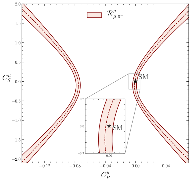
Figure 5: Allowed regions in the $C^{\mu}_{P}$–$C^{\mu}_{S}$ plane using the ratios $\mathcal{R}^{\mu}_{\mu;\pi^{0}}$ (left) and $\mathcal{R}^{\mu}_{\mu;\pi^{-}}$ (right).

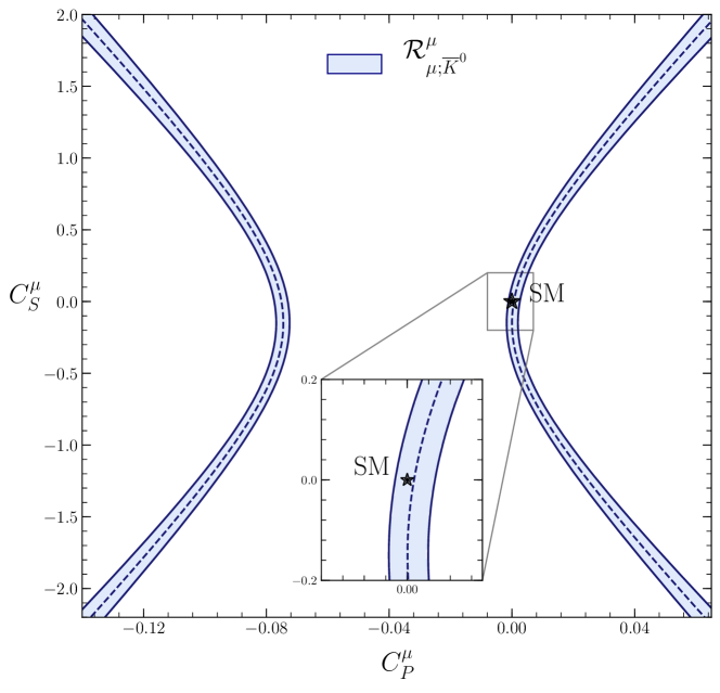
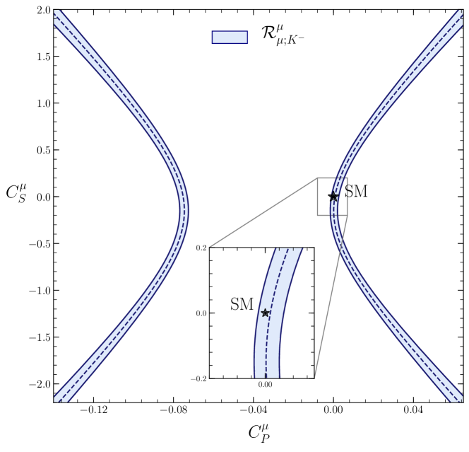
Figure 6: Allowed regions in the $C^{\mu}_{P}$–$C^{\mu}_{S}$ plane using the ratios $\mathcal{R}^{\mu}_{\mu;\overline{K}^{0}}$ (left) and $\mathcal{R}^{\mu}_{\mu;K^{-}}$ (right).

4.1.2 Constraints on Vector Coefficients

Next, we consider contributions from LH and RH vector NP interactions. The differential branching fraction can be written as follows:

$$\begin{split}\frac{d\mathcal{B}(D\rightarrow P\bar{\ell}\nu_{\ell})}{dq^{2}}&=\frac{d\mathcal{B}(D\rightarrow P\bar{\ell}\nu_{\ell})}{dq^{2}}\Bigg{|}_{\text{SM}}\Big{|}1+C^{\ell}_{V_{L(R)}}\Big{|}^{2}.\end{split}$$ (33)

In principle, we could define ratios in analogy to Eqs. (29) and (30) given in the previous section, but include vector contributions instead of (pseudo)-scalar ones. However, Eqs. (22) and (33) indicate that the LH vector NP contributions would cancel. On the other hand, in the case of RH vector contributions, they would not cancel due to the relative sign difference, but the structure of the formulae does prohibit the extraction of stringent constraints.

We can, however, investigate possible vector NP interactions through ratios between two semileptonic decays with different flavours of leptons. To this end, we define the following observables:

$$\mathcal{R}^{e}_{\mu;\pi^{0}}\equiv\frac{\mathcal{B}(D^{+}\to\pi^{0}e^{+}\nu_{e})}{\mathcal{B}(D^{+}\to\pi^{0}\mu^{+}\nu_{\mu})},\hskip 28.45274pt\mathcal{R}^{e}_{\mu;\pi^{-}}\equiv\frac{\mathcal{B}(D^{0}\to\pi^{-}e^{+}\nu_{e})}{\mathcal{B}(D^{0}\to\pi^{-}\mu^{+}\nu_{\mu})},$$ (34)

and

$$\mathcal{R}^{e}_{\mu;\overline{K}^{0}}\equiv\frac{\mathcal{B}(D^{+}\to\overline{K}^{0}e^{+}\nu_{e})}{\mathcal{B}(D^{+}\to\overline{K}^{0}\mu^{+}\nu_{\mu})},\hskip 28.45274pt\mathcal{R}^{e}_{\mu;K^{-}}\equiv\frac{\mathcal{B}(D^{0}\to K^{-}e^{+}\nu_{e})}{\mathcal{B}(D^{0}\to K^{-}\mu^{+}\nu_{\mu})}.$$ (35)

These observables are independent of CKM matrix elements and sensitive to the coefficients $C^{\ell}_{V_{L(R)}}$, with $\ell=e,\mu$. Hence, they provide interesting opportunities to test lepton flavour universality in $D$ decays. From the measured branching fractions in Table 2, we obtain the following experimental values:

$$\mathcal{R}^{e}_{\mu;\pi^{0}}=1.06\pm 0.07,\hskip 28.45274pt\mathcal{R}^{e}_{\mu;\pi^{-}}=1.09\pm 0.05,$$ (36)

and

$$\mathcal{R}^{e}_{\mu;\overline{K}^{0}}=(9.97\pm 0.24)\times 10^{-1},\hskip 28.45274pt\mathcal{R}^{e}_{\mu;K^{-}}=1.04\pm 0.01.$$ (37)

The structure of the theoretical expressions for these observables, following from Eq. (33), is identical for LH and RH vector NP interactions. Therefore, the allowed regions in the $C^{\mu}_{V_{L}}$–$C^{e}_{V_{L}}$ and $C^{\mu}_{V_{R}}$–$C^{e}_{V_{R}}$ planes, obtained by comparing these expression with the experimental values, are the same. This is can be seen in Figs. 7 and 8. Furthermore, as leptonic and semileptonic decays are described by the same operators, we may compare these constraints with the ones obtained from leptonic decays in Fig. 3 (right) and Fig. 4 (right). The constraints presented there are a significant improvement, resulting from the fact that semileptonic decays do not suffer from helicity suppression. It is interesting to note that the SM predictions, $C^{\mu}_{V_{L(R)}}=C^{e}_{V_{L(R)}}=0$, lie just outside the 1$\sigma$ contours in three of the four plots.

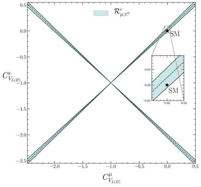
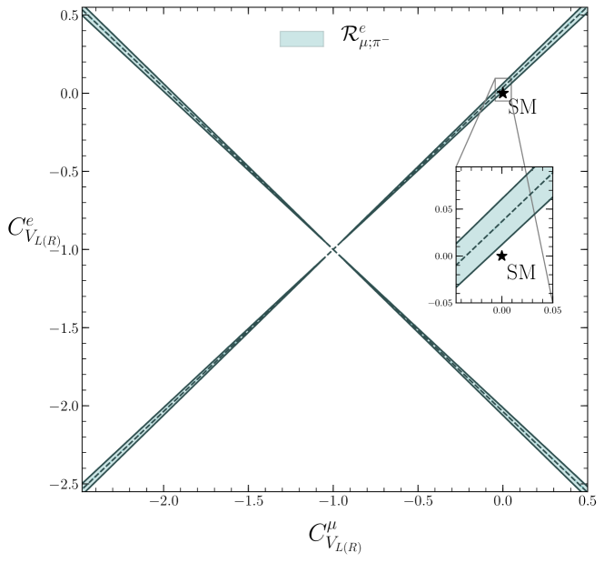
Figure 7: Allowed regions in the $C^{\mu}_{V_{L(R)}}$–$C^{e}_{V_{L(R)}}$ plane using the ratios $\mathcal{R}^{\mu}_{\mu;\pi^{0}}$ (left) and $\mathcal{R}^{\mu}_{\mu;\pi^{-}}$ (right).

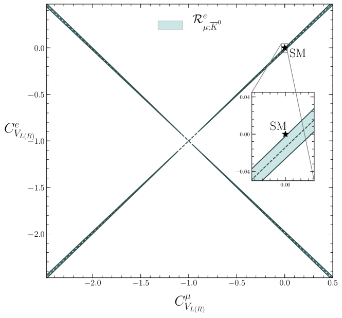
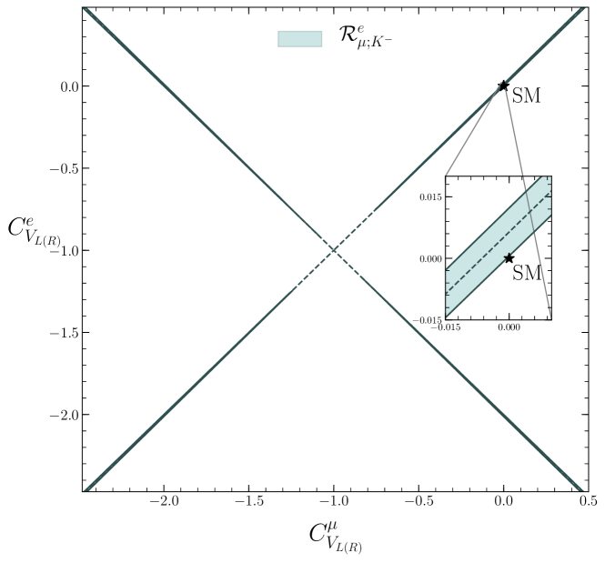
Figure 8: Allowed regions in the $C^{\mu}_{V_{L(R)}}$–$C^{e}_{V_{L(R)}}$ plane using the ratios $\mathcal{R}^{\mu}_{\mu;\overline{K}^{0}}$ (left) and $\mathcal{R}^{\mu}_{\mu;K^{-}}$ (right).

4.1.3 Constraints on Tensor Coefficients

Finally, let us probe the tensor operator in the operator basis given in Eq. (2) through its impact on the semileptonic decays. The differential branching fraction including such tensor interactions is given as

$$\begin{split}\frac{d\mathcal{B}(D\rightarrow P\bar{\ell}\nu_{\ell})}{dq^{2}}&=\frac{G_{F}^{2}\tau_{D}|V_{cq}|^{2}}{24\pi^{3}M_{D}^{2}}\Bigg{\{}\Bigg{[}\frac{(H^{P}_{V,0})^{2}}{4}\Big{(}1+\frac{m_{\ell}^{2}}{2q^{2}}\Big{)}+\frac{3}{8}\frac{m_{\ell}^{2}}{q^{2}}(H^{P}_{V,t})^{2}\Bigg{]}\\ &\hskip 14.22636pt+2|C_{T}^{\ell}|^{2}\Big{(}1+\frac{2m_{\ell}^{2}}{q^{2}}\Big{)}(H^{P}_{T})^{2}-3\mathcal{R}e(C_{T}^{\ell*})\frac{m_{\ell}}{\sqrt{q^{2}}}H^{P}_{T}H^{P}_{V,0}\Bigg{\}}\frac{(q^{2}-m_{\ell}^{2})^{2}}{q^{2}}|\vec{p}_{P}|.\end{split}$$ (38)

For the amplitude $H^{P}_{T}$, we use the lattice results obtained in Ref. [41] for the corresponding form factors (for details, see Appendix A). This leads to expressions for the semileptonic branching fractions, dependent on the tensor NP coefficients $C^{\ell}_{T}$. As the tensor operator in Eq. (2) is antisymmetric in $\mu$ and $\nu$, there are no tensor contributions to leptonic decays. Consequently, we cannot probe tensor NP through ratios between leptonic and semileptonic decays. Hence, we take the ratios in Eqs. (34) and (35), but allow for tensor contributions instead of vector contributions. These ratios are then sensitive to the tensor coefficients $C^{e}_{T}$ and $C^{\mu}_{T}$.

By comparing our theoretical expressions with the experimental information in Eqs. (36) and (37), we determine the allowed regions in the $C^{\mu}_{T}$–$C^{e}_{T}$ plane. The constraints from $\mathcal{R}^{e}_{\mu;\pi^{0}}$ and $\mathcal{R}^{e}_{\mu;\pi^{-}}$ are shown in the panels on the left- and right-hand sides of Fig. 9, respectively. In the latter case, it is interesting to see that the SM prediction corresponding to $C^{\mu}_{T}=C^{e}_{T}=0$ is excluded at the 1 $\sigma$ level. In Fig. 10, the allowed regions in the $C^{\mu}_{T}$–$C^{e}_{T}$ plane are shown, following from the constraints on $\mathcal{R}^{e}_{\mu;\overline{K}^{0}}$ (left) and $\mathcal{R}^{e}_{\mu;K^{-}}$ (right). We observe that in the case of $\mathcal{R}^{e}_{\mu;\overline{K}^{0}}$, the SM prediction lies just outside the 1 $\sigma$ contours.

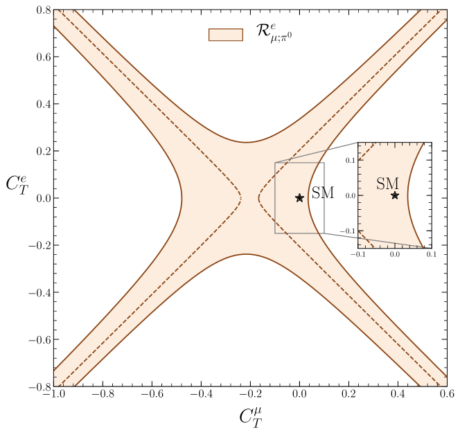
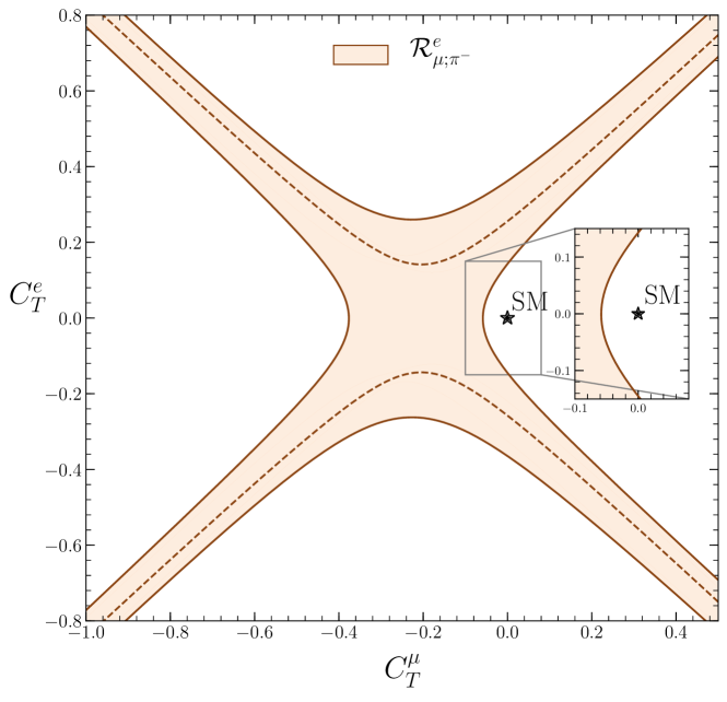
Figure 9: Allowed regions in the $C^{\mu}_{T}-C^{e}_{T}$ plane using the ratios $\mathcal{R}^{e}_{\mu;\pi^{0}}$ (left) and $\mathcal{R}^{e}_{\mu;\pi^{-}}$ (right).

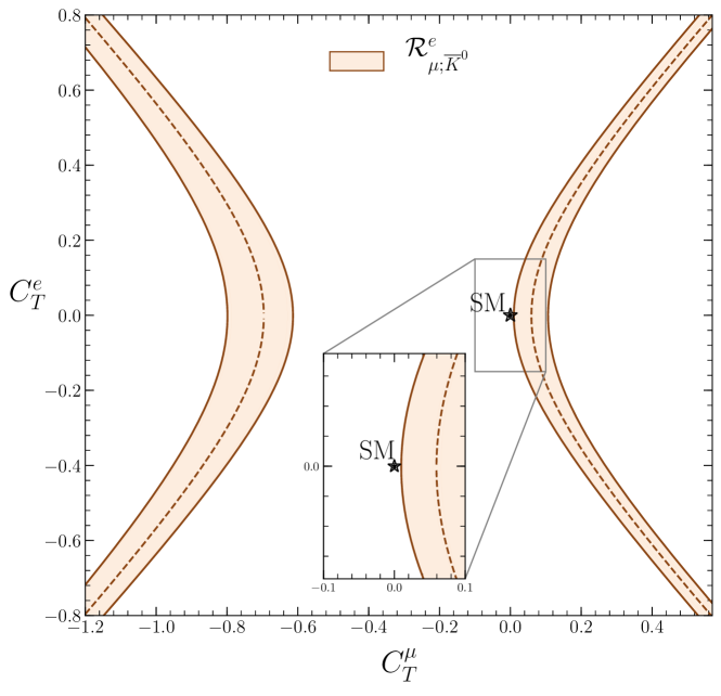
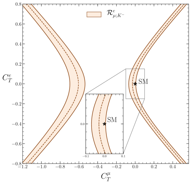
Figure 10: Allowed regions in the $C^{\mu}_{T}-C^{e}_{T}$ plane using the ratios $\mathcal{R}^{e}_{\mu;\overline{K}^{0}}$ (left) and $\mathcal{R}^{e}_{\mu;K^{-}}$ (right).

4.2 $D\to V\bar{\ell}\nu_{\ell}$ Decays

We continue our analysis of semileptonic $D_{(s)}$ decays by considering decays of the form $D\to V\bar{\ell}\nu_{\ell}$, where $V$ denotes a vector meson. Measurements of the branching fractions for $D\to\rho$ and $D\to K^{*}$ decays allow us to further constrain the short-distance NP coefficients. In particular, $D\to V$ decays are sensitive to the pseudoscalar NP coefficient $C_{P}^{\ell}$, thereby offering an interesting complement to the constraints following from the leptonic decays in Section 3.

The SM expression for the differential branching fraction for $D\rightarrow V\bar{\ell}\nu_{\ell}$ decays takes the form [25]

$$\begin{split}\frac{d\mathcal{B}(D\rightarrow V\bar{\ell}\nu_{\ell})}{dq^{2}}&=\frac{G_{F}^{2}\tau_{D}|V_{cq}|^{2}}{24\pi^{3}M^{2}_{D}}\Bigg{\{}\frac{1}{4}\Big{(}1+\frac{m_{\ell}^{2}}{2q^{2}}\Big{)}\Big{[}(H^{V}_{V,+})^{2}+(H^{V}_{V,-})^{2}+(H^{V}_{V,0})^{2}\Big{]}\\ &\hskip 71.13188pt+\frac{3}{8}\frac{m_{\ell}^{2}}{q^{2}}(H^{V}_{V,t})^{2}\Bigg{\}}\frac{(q^{2}-m_{\ell}^{2})^{2}}{q^{2}}|\vec{p}_{V}|,\end{split}$$ (39)

where $q^{2}$ has the kinematical range

$$m_{\ell}^{2}\leq q^{2}\leq(M_{D}-M_{V})^{2}.$$ (40)

In comparison with the pseudoscalar case, we have now a considerably more complex situation due to the amplitudes $H^{V}_{V,+}$, $H^{V}_{V,-}$, $H^{V}_{V,0}$ and $H^{V}_{V,t}$, which involve various hadronic form factors. Unfortunately, to the best of our knowledge, the most recent lattice calculation of the $D\to\rho,K^{*}$ form factors dates back to 1995 [42]. As significant improvements have recently been made in lattice QCD, a calculation of the $D\to V$ form factors exploiting the current state-of-the-art methods would be very desirable for testing LFU in the charm sector.

In our work, we complement the lattice QCD (LQCD) calculation in Ref. [42] with the results from Ref. [43], using light-cone sum rules (LCSR). The latter calculation is done in the framework of Heavy Quark Effective Field Theory (HQEFT). It should be mentioned that HQEFT, as the name suggests, relies on the assumption of a heavy quark, which in the case of $D$ mesons has to be treated carefully [44]. The definitions and different parametrizations of the form factors are given in Appendix A. The resulting SM predictions for the branching fractions and the corresponding experimental results are summarized in Table 3. For the SM predictions, we use the values for $|V_{cd}|$ and $|V_{cs}|$ in Eqs. (10) and (11), respectively.

Decay	LQCD	LCSR	Experiment
$\mathcal{B}(D^{+}\to\rho^{0}e^{+}\nu_{e})$	$(2.23\pm 0.70)\times 10^{-3}$	$(2.25\pm 0.28)\times 10^{-3}$	$(2.18^{+0.17}_{-0.25})\times 10^{-3}$
$\mathcal{B}(D^{+}\to\overline{K}^{*}(892)^{0}e^{+}\nu_{e})$	$(6.26\pm 1.84)\times 10^{-2}$	$(5.02\pm 0.56)\times 10^{-2}$	$(5.40\pm 0.10)\times 10^{-2}$
$\mathcal{B}(D^{+}\to\rho^{0}\mu^{+}\nu_{\mu})$	$(2.13\pm 0.64)\times 10^{-3}$	$(2.14\pm 0.27)\times 10^{-3}$	$(2.4\pm 0.4)\times 10^{-3}$
$\mathcal{B}(D^{+}\to\overline{K}^{*}(892)^{0}\mu^{+}\nu_{\mu})$	$(5.95\pm 1.67)\times 10^{-2}$	$(4.75\pm 0.53)\times 10^{-2}$	$(5.27\pm 0.15)\times 10^{-2}$

Table 3: SM predictions for $D\to V\bar{\ell}\nu_{\ell}$ branching ratios using LQCD and LCSR form-factor information from Refs. [42] and [43], respectively; the experimental values are from Ref. [30].

4.2.1 Constraints on Pseudoscalar Coefficients

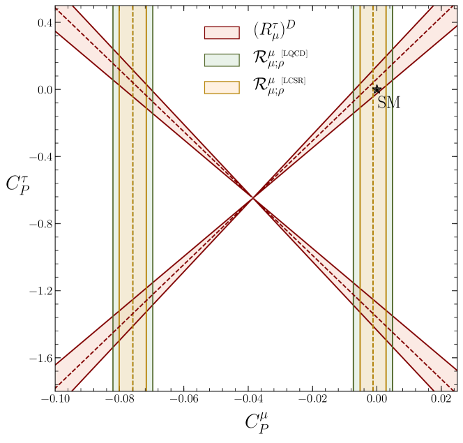
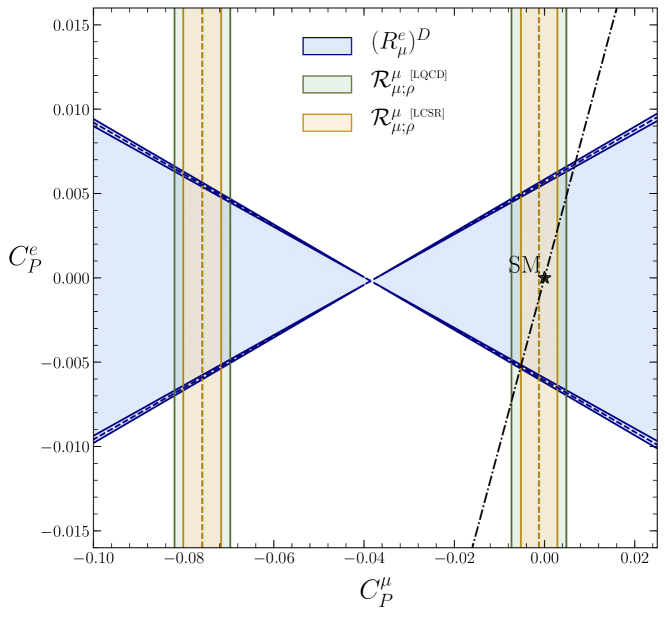
Figure 11: Allowed regions in the $C^{\mu}_{P}$–$C^{\tau}_{P}$ (left) and $C^{\mu}_{P}$–$C^{e}_{P}$ (right) planes using the ratios $(R^{\tau}_{\mu})^{D}$, $\mathcal{R}^{\mu}_{\mu;\rho}$ and $(R^{e}_{\mu})^{D}$, $\mathcal{R}^{\mu}_{\mu;\rho}$, respectively. The dashed-dotted line corresponds to $C^{e}_{P}=C^{\mu}_{P}$.

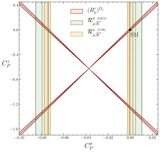
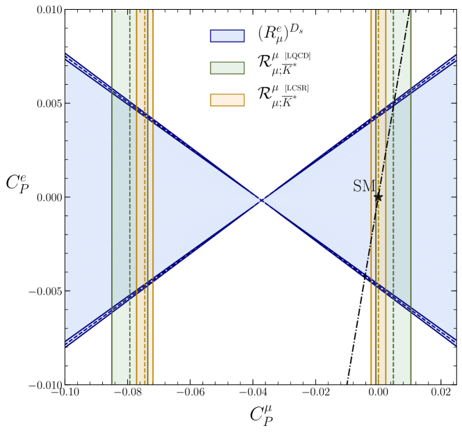
Figure 12: Allowed regions in the $C^{\mu}_{P}$–$C^{\tau}_{P}$ (left) and $C^{\mu}_{P}$–$C^{e}_{P}$ (right) planes using the ratios $(R^{\tau}_{\mu})^{D_{s}}$, $\mathcal{R}^{\mu}_{\mu;\overline{K}^{*}}$ and $(R^{e}_{\mu})^{D_{s}}$, $\mathcal{R}^{\mu}_{\mu;\overline{K}^{*}}$, respectively. The dashed-dotted line corresponds to $C^{e}_{P}=C^{\mu}_{P}$.

If we allow for pseudoscalar NP interactions, we obtain the following expression for the differential branching fraction for semileptonic $D$ decays with vector mesons in the final state:

$$\begin{split}&\frac{d\mathcal{B}(D\rightarrow V\bar{\ell}\nu_{\ell})}{dq^{2}}=\frac{G_{F}^{2}\tau_{D}|V_{cq}|^{2}}{24\pi^{3}M^{2}_{D}}\Bigg{\{}\Bigg{[}\frac{1}{4}\Big{(}1+\frac{m_{\ell}^{2}}{2q^{2}}\Big{)}\Big{[}(H^{V}_{V,+})^{2}+(H^{V}_{V,-})^{2}+(H^{V}_{V,0})^{2}\Big{]}\\ &+\frac{3}{8}\frac{m_{\ell}^{2}}{q^{2}}(H^{V}_{V,t})^{2}\Bigg{]}+\frac{3}{8}|C_{P}^{\ell}|^{2}(H^{V}_{S})^{2}+\frac{3}{4}\mathcal{R}e(C_{P}^{\ell*})\frac{m_{\ell}}{\sqrt{q^{2}}}H^{V}_{S}H^{V}_{V,t}\Bigg{\}}\frac{(q^{2}-m_{\ell}^{2})^{2}}{q^{2}}|\vec{p}_{V}|,\end{split}$$ (41)

where the terms in the large square brackets represent the SM part. In order to constrain the pseudoscalar NP coefficients $C^{\ell}_{P}$, we introduce the ratios

$$\begin{split}\mathcal{R}^{\mu}_{\mu;\rho}&=\frac{\mathcal{B}(D^{+}\to\mu^{+}\nu_{\mu})}{\mathcal{B}(D^{+}\to\rho^{0}\mu^{+}\nu_{\mu})},\hskip 28.45274pt\mathcal{R}^{\mu}_{\mu;\overline{K}^{*}}=\frac{\mathcal{B}(D_{s}^{+}\to\mu^{+}\nu_{\mu})}{\mathcal{B}(D^{+}\to\overline{K}^{*}(892)^{0}\mu^{+}\nu_{\mu}}.\end{split}$$ (42)

Since each of these observables depends on $C^{\mu}_{P}$, they can be used to complement the constraints for this coefficient following from the leptonic $D$ decays. Note that for the $D^{+}\to\rho^{0}\mu^{+}\nu_{\mu}$ channel, a factor of 1/2 has to be taken into account due to the wave function of the $\rho^{0}$ meson. Using the measured branching fractions in Table 3, we obtain the following experimental values:

$$\begin{split}\mathcal{R}^{\mu}_{\mu;\rho}&=(1.56\pm 0.27)\times 10^{-1},\hskip 28.45274pt\mathcal{R}^{\mu}_{\mu;\overline{K}^{*}}=(1.04\pm 0.05)\times 10^{-1}.\\ \end{split}$$ (43)

These constraints can be converted correspondingly into allowed ranges for $C^{\mu}_{P}$, employing $c\to d$ and $c\to s$ transitions. The results are listed in Table 4, utilizing information on the form factors both from LQCD and from LCSR calculations.

Coefficient	LQCD	LCSR
$C^{\mu}_{P}\big{|}_{cd}$	$(-7.58\pm 0.62)\times 10^{-2}$	$(-7.59\pm 0.42)\times 10^{-2}$
	$(-1.23\pm 6.08)\times 10^{-3}$	$(-1.19\pm 4.04)\times 10^{-3}$
$C^{\mu}_{P}\big{|}_{cs}$	$(-7.93\pm 0.57)\times 10^{-2}$	$(-7.45\pm 0.26)\times 10^{-2}$
	$(4.82\pm 5.59)\times 10^{-3}$	$(0.05\pm 2.34)\times 10^{-3}$

Table 4: Allowed values for the coefficients $C^{\mu}_{P}\big{|}_{cd}$ and $C^{\mu}_{P}\big{|}_{cs}$, obtained through the ratios $\mathcal{R}^{\mu}_{\mu;\rho}$ and $\mathcal{R}^{\mu}_{\mu;\overline{K}^{*}}$, respectively, using LQCD [42] and LCSR [43] form-factor information.

We may use the obtained ranges for $C^{\mu}_{P}$ to further constrain the allowed regions shown in Figs. 1 and 2. This yields the vertical bands in Figs. 11 and 12. The constraints obtained using LQCD and LCSR form-factor information are indicated by the green and yellow bands, respectively. The dashed-dotted lines in Figs. 11 (right) and 12 (right) indicate the correlations arising from $C^{e}_{P}=C^{\mu}_{P}$. In both cases, we find no large discrepancies with the SM predictions where the pseudoscalar NP coefficients vanish.

4.2.2 Constraints on Vector Coefficients

Besides pseudoscalar NP interactions, semileptonic $D$ decays with a vector meson in the final state are also sensitive probes of LH and RH vector contributions from physics beyond the SM. The differential branching fraction in the presence of LH vector NP interactions can be written as

$$\begin{split}\frac{d\mathcal{B}(D\rightarrow V\bar{\ell}\nu_{\ell})}{dq^{2}}=\frac{d\mathcal{B}(D\rightarrow V\bar{\ell}\nu_{\ell})}{dq^{2}}\Bigg{|}_{\text{SM}}\big{|}1+C_{V_{L}}|^{2}.\end{split}$$ (44)

In analogy to decays with pseudoscalar mesons in the final states, the ratio between a leptonic and semileptonic decay does not yield further constraints since the additional LH vector contributions cancel. The differential branching fraction in the presence of RH vector NP interactions is slightly different from the pseudoscalar case [25]:

$$\begin{split}&\frac{d\mathcal{B}(D\rightarrow V\bar{\ell}\nu_{\ell})}{dq^{2}}=\frac{G_{F}^{2}\tau_{D}|V_{cq}|^{2}}{24\pi^{3}M^{2}_{D}}\Bigg{\{}\Bigg{[}\frac{1}{4}\Big{(}1+\frac{m_{\ell}^{2}}{2q^{2}}\Big{)}\Big{[}(H^{V}_{V,+})^{2}+(H^{V}_{V,-})^{2}+(H^{V}_{V,0})^{2}\Big{]}\\ &+\frac{3}{8}\frac{m_{\ell}^{2}}{q^{2}}(H^{V}_{V,t})^{2}\Bigg{]}(1+|C^{\ell}_{V_{R}}|^{2})-2\mathcal{R}e(C_{V_{R}}^{\ell*})\Bigg{[}\frac{1}{4}\Big{(}1+\frac{m_{\ell}^{2}}{2q^{2}}\Big{)}\Big{[}(H^{V}_{V,0})^{2}+2H^{V}_{V,+}H^{V}_{V,-}\Big{]}\\ &+\frac{3}{8}\frac{m_{\ell}^{2}}{q^{2}}(H^{V}_{V,t})^{2}\Bigg{]}\Bigg{\}}\frac{(q^{2}-m_{\ell}^{2})^{2}}{q^{2}}|\vec{p}_{V}|.\end{split}$$ (45)

However, the structure of the formulae does prohibit the extractions of further constraints through the ratio between a leptonic and a semileptonic decay with the same lepton flavour. Therefore, in analogy to Eqs. (34) and (35), we define the following ratios between two semileptonic decays with different flavours of leptons:

$$\mathcal{R}^{e}_{\mu;\rho}\equiv\frac{\mathcal{B}(D^{+}\to\rho^{0}e^{+}\nu_{e})}{\mathcal{B}(D^{+}\to\rho^{0}\mu^{+}\nu_{\mu})},\hskip 28.45274pt\mathcal{R}^{e}_{\mu;\overline{K}^{*}}\equiv\frac{\mathcal{B}(D^{+}\to\overline{K}^{*}(892)^{0}e^{+}\nu_{e})}{\mathcal{B}(D^{+}\to\overline{K}^{*}(892)^{0}\mu^{+}\nu_{\mu})}.$$ (46)

From the measured branching fractions in Table 3, we obtain the following experimental constraints:

$$\mathcal{R}^{e}_{\mu;\rho}=(9.08\pm 1.75)\times 10^{-1},\hskip 28.45274pt\mathcal{R}^{e}_{\mu;\overline{K}^{*}}=1.02\pm 0.03.$$ (47)

By comparing Eqs. (33) and (44) with each other, it is clear that the contours in the $C^{\mu}_{V_{L}}$–$C^{e}_{V_{L}}$ planes will be of the same shape; the expressions differ only up to a scale-factor. As the form-factor information for $D\to P$ decays is significantly more precise than for $D\to V$ decays, and the experimental precision is more or less the same, the constraints coming from $D\to V$ decays do not improve the constraints in Figs. 7 and 8. For RH vector interactions, however, the slightly different structure is worth investigating. For $\mathcal{R}^{e}_{\mu;\rho},$ this leads to the contour shown in Fig. 13 (left), and for $\mathcal{R}^{e}_{\mu;\overline{K}^{*}}$, this leads to the contour shown in Fig. 13 (right). In both plots, the SM prediction is included in the 1$\sigma$ contours.

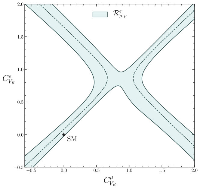
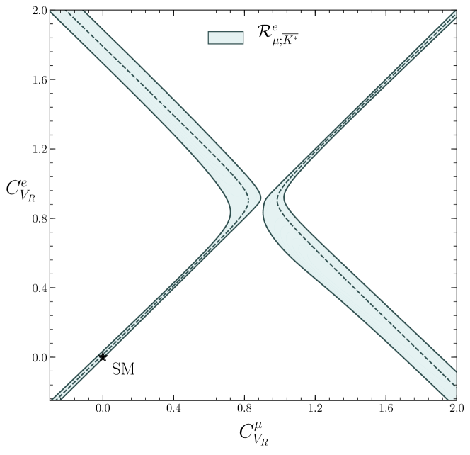
Figure 13: Allowed regions in the $C^{\mu}_{V_{R}}$–$C^{e}_{V_{R}}$ plane using the ratios $\mathcal{R}^{e}_{\mu;\rho}$ (left) and $\mathcal{R}^{e}_{\mu;\overline{K}^{*}}$ (right).

4.2.3 Constraints on Tensor Coefficients

Finally, let us have a closer look at NP tensor contributions, which are the final category of potential NP contributions to semileptonic $D$ decays with a vector meson in the final state. Allowing for such an effect, we obtain the following differential branching ratio:

$$\begin{split}&\frac{d\mathcal{B}(D\rightarrow V\bar{\ell}\nu_{\ell})}{dq^{2}}=\frac{G_{F}^{2}\tau_{D}|V_{cq}|^{2}}{24\pi^{3}M^{2}_{D}}\Bigg{\{}\Bigg{[}\frac{1}{4}\Big{(}1+\frac{m_{\ell}^{2}}{2q^{2}}\Big{)}\Big{[}(H^{V}_{V,+})^{2}+(H^{V}_{V,-})^{2}+(H^{V}_{V,0})^{2}\Big{]}\\ &+\frac{3}{8}\frac{m_{\ell}^{2}}{q^{2}}(H^{V}_{V,t})^{2}\Bigg{]}+2|C^{\ell}_{T}|^{2}\Big{(}1+\frac{2m_{\ell}^{2}}{q^{2}}\Big{)}\Big{[}(H^{V}_{T,+})^{2}+(H^{V}_{T,-})^{2}+(H^{V}_{T,0})^{2}\Big{]}\\ &-3\mathcal{R}e(C^{\ell*}_{T})\frac{m_{\ell}}{\sqrt{q^{2}}}\big{(}H^{V}_{T,0}H^{V}_{V,0}+H^{V}_{T,+}H^{V}_{V,-}-H^{V}_{T,-}H^{V}_{V,+}\big{)}\Bigg{\}}\frac{(q^{2}-m_{\ell}^{2})^{2}}{q^{2}}|\vec{p}_{V}|.\end{split}$$ (48)

However, to the best of our knowledge, there is no explicit lattice calculation of the tensor form factors for $D\to V$ decays available. In Ref. [43], the tensor form factors are related to the vector and scalar form factors $A_{1}$, $A_{2}$, $A_{3}$, $V$ in the framework of HQEFT. A lattice determination of the tensor form factors in $D\to V$ transitions would be very desirable. However, as currently no lattice information is available for these quantities, we will use the HQEFT relations to obtain constraints, albeit for illustrative purpose. The relations for the form factors are given as follows [43]:

$$T_{1}(q^{2}) =\frac{M_{D}^{2}-m_{V}^{2}+q^{2}}{2M_{D}}\frac{V(q^{2})}{M_{D}+m_{V}}+\frac{M_{D}+m_{V}}{2M_{D}}A_{1}(q^{2}),$$ (49)

$$T_{2}(q^{2}) =\frac{2}{M_{D}^{2}-m_{V}^{2}}\Bigg{[}\frac{(M_{D}-y)(M_{D}+m_{V})}{2}A_{1}(q^{2})+\frac{M_{D}(y^{2}-m_{V}^{2})}{M_{D}+m_{V}}V(q^{2})\Bigg{]},$$ (50)

$$T_{3}(q^{2}) =-\frac{M_{D}+m_{V}}{2M_{D}}A_{1}(q^{2})+\frac{M_{D}-m_{V}}{2M_{D}}\big{[}A_{2}(q^{2})-A_{3}(q^{2})\big{]}+\frac{M_{D}^{2}+3m_{V}^{2}-q^{2}}{2M_{D}(M_{D}+m_{V})}V(q^{2}).$$ (51)

where $y=(M_{D}^{2}+m_{V}^{2}-q^{2})/(2M_{D})$ is the energy of the vector meson. We use the ratios defined in Eq. (46) and allow for tensor contributions instead of vector contributions. Using the HQEFT relations and the experimental information, we find the allowed regions in the $C^{\mu}_{T}$–$C^{e}_{T}$ plane shown in Fig. 14. We observe that the SM points fall just within in the 1 $\sigma$ regions in both cases.

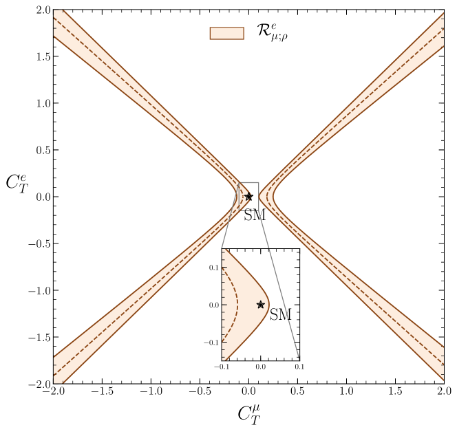
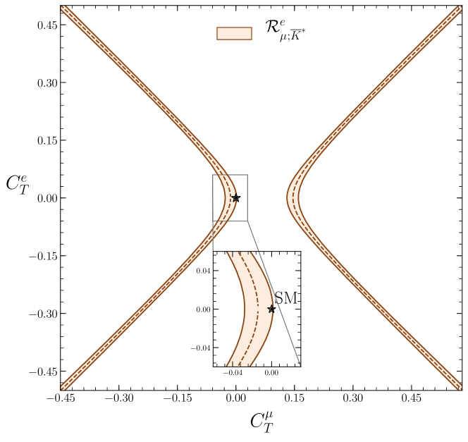
Figure 14: Allowed regions in the $C^{\mu}_{T}$–$C^{e}_{T}$ plane using the ratios $\mathcal{R}^{\mu}_{\mu;\rho}$ (left) and $\mathcal{R}^{\mu}_{\mu;\overline{K}^{*}}$ (right).

5 Determination of $|V_{cd}|$ and $|V_{cs}|$

The determination of $|V_{cd}|$ or $|V_{cs}|$ is done by exploiting data from charged-current interactions involving $c\to d\bar{\ell}\nu_{\ell}$ or $c\to s\bar{\ell}\nu_{\ell}$ quark-level transitions, respectively. Usually, these determinations assume just the corresponding SM expressions. However, there may be NP contributions present in these processes, as is the main focus of our analysis. In the case of (semi)-leptonic $D_{(s)}$ decays, their SM expressions could be used to determine $|V_{cd(s)}|$ from the data and non-perturbative information on the hadronic parameters. In Section 2.2, we have determined $|V_{cd(s)}|$ independently of $D_{(s)}$ decays, utilizing the Wolfenstein parametrization of the CKM matrix. Here, we have assumed the SM in the corresponding kaon and $B$ decay processes.

Physics beyond the SM may also affect the values of the CKM matrix elements. Consequently, we have probed NP through observables that do not involve such parameters. Combining the theoretical expressions for these observables with experimental information on the branching fractions allows us to constrain NP coefficients, independently of the CKM matrix elements. Finally, having these constraints available, we may use them to extract $|V_{cd(s)}|$ from $D_{(s)}$ decays, even in the presence of possible NP effects in the corresponding transition amplitudes.

5.1 The Strategy

In our analysis, we follow a strategy first proposed for $B$ decays in Ref. [22]. It has not yet been applied to the charm sector. Using the NP constraints obtained from the observables $\mathcal{R}^{\mu}_{\mu;\rho}$ and $\mathcal{R}^{\mu}_{\mu;\overline{K}^{*}}$, we will finally also determine $|V_{cd}|$ or $|V_{cs}|$ in the presence of pseudoscalar NP contributions. To distinguish the coefficients corresponding either to a $c\to d$ transition or a $c\to s$ transition, we denote the latter with $\tilde{C}^{\mu}_{P}$. There are three steps in this approach, after which we obtain the CKM matrix elements:

• We start with the expressions for $\mathcal{R}^{\mu}_{\mu;\rho}$ and $\mathcal{R}^{\mu}_{\mu;\overline{K}^{*}}$ in Eq. (42), which depend only on one coefficient, either $C^{\mu}_{P}$ or $\tilde{C}^{\mu}_{P}$. Consequently, we can solve for $C^{\mu}_{P}$ or $\tilde{C}^{\mu}_{P}$.

• This results in the functions $C^{\mu}_{P}(\mathcal{R}^{\mu}_{\mu;\rho})$ and $\tilde{C}^{\mu}_{P}(\mathcal{R}^{\mu}_{\mu;\overline{K}^{*}})$. For both functions, there are two independent solutions for the coefficients, corresponding to the two bands shown in Figs. 11 and 12.

• We then evaluate any of the individual branching fractions for each of these ratios and solve for the corresponding CKM matrix element. Comparing the resulting expression to individual measurements of the branching fractions allows us to obtain the value of $|V_{cd}|$ or $|V_{cs}|$.

5.2 $|V_{cd}|$ and $|V_{cs}|$

We apply the described strategy to leptonic and semileptonic $D_{(s)}$ decays to determine the CKM matrix elements $|V_{cd}|$ and $|V_{cs}|$. To this end, we recall the following ratios:

$$\begin{split}\mathcal{R}^{\mu}_{\mu;\rho}&=\frac{\mathcal{B}(D^{+}\to\mu^{+}\nu_{\mu})}{\mathcal{B}(D^{+}\to\rho^{0}\mu^{+}\nu_{\mu})},\hskip 28.45274pt\mathcal{R}^{\mu}_{\mu;\overline{K}^{*}}=\frac{\mathcal{B}(D_{s}^{+}\to\mu^{+}\nu_{\mu})}{\mathcal{B}(D^{+}\to\overline{K}^{*}(892)^{0}\mu^{+}\nu_{\mu}},\\ \end{split}$$ (52)

which were given in Section 4.2.2, along with the theoretical expressions for the branching fractions including pseudoscalar NP contributions. Using these expressions, we write the ratios as follows:

$$\mathcal{R}^{\ell}_{\ell;V}=\frac{\tilde{\alpha}^{\ell}\Big{|}1+\beta^{\ell}C^{\ell}_{P}\Big{|}^{2}}{\mathcal{I}_{1}+\mathcal{I}_{2}|C_{P}^{\ell}|^{2}+\mathcal{I}_{3}\mathcal{R}e(C_{P}^{\ell*})},$$ (53)

where $V=\rho,\overline{K}^{*}$ and $\tilde{\alpha}^{\ell}=\alpha^{\ell}f_{D}^{2}$. To keep the notation clear, the subscript $s$ is omitted; in the case $\mathcal{R}^{\mu}_{\mu;\overline{K}^{*}}$ the notation $D\to D_{s}$ and $C^{\ell}_{P}\to\tilde{C}^{\ell}_{P}$ is implied. The integrals $\mathcal{I}_{1}$, $\mathcal{I}_{2}$, $\mathcal{I}_{3}$ take the forms

$$\begin{split}\mathcal{I}_{1}&=I_{0}\int_{m_{\ell}^{2}}^{(M_{D}-m_{V})^{2}}dq^{2}\Bigg{[}\frac{1}{4}\Big{(}1+\frac{m_{\ell}^{2}}{2q^{2}}\Big{)}\Big{[}(H^{+}_{V})^{2}+(H_{V}^{-})^{2}+(H_{V}^{0})^{2}\Big{]}+\frac{3}{8}\frac{m_{\ell}^{2}}{q^{2}}(H^{t}_{V})^{2}\Bigg{]}\frac{(q^{2}-m_{\ell}^{2})^{2}}{q^{2}}|\vec{p}_{V}|,\\ \mathcal{I}_{2}&=I_{0}\int_{m_{\ell}^{2}}^{(M_{D}-m_{V})^{2}}dq^{2}\frac{3}{8}(H^{0}_{P})^{2}\frac{(q^{2}-m_{\ell}^{2})^{2}}{q^{2}}|\vec{p}_{V}|,\\ \mathcal{I}_{3}&=I_{0}\int_{m_{\ell}^{2}}^{(M_{D}-m_{V})^{2}}dq^{2}\frac{3}{4}\frac{m_{\ell}}{\sqrt{q^{2}}}H^{0}_{P}H^{t}_{V}\frac{(q^{2}-m_{\ell}^{2})^{2}}{q^{2}}|\vec{p}_{V}|,\end{split}$$ (54)

where $I_{0}=1/(3\pi^{2}M^{2}_{D})$. Note that for $\mathcal{R}^{\mu}_{\mu;\overline{K}^{*}}$, an additional factor of $\tau_{D_{s}}/\tau_{D}$ should be included, as the decaying D mesons in the leptonic and semileptonic decays are different. We assume the coefficients to be real and solve for $C^{\mu}_{V_{R}}$, $\tilde{C}^{\mu}_{V_{R}}$. The resulting expressions are the functions $C^{\mu}_{P}(\mathcal{R}^{\mu}_{\mu;\rho})$ and $\tilde{C}^{\mu}_{P}(\mathcal{R}^{\mu}_{\mu;\overline{K}^{*}})$. Subsequently, we insert $C^{\mu}_{P}(\mathcal{R}^{\mu}_{\mu;\rho})$ and $\tilde{C}^{\mu}_{P}(\mathcal{R}^{\mu}_{\mu;\overline{K}^{*}})$ in the expressions for the (semi)-leptonic branching fractions and solve for the corresponding CKM element. For the leptonic branching fractions, this yields:

$$\begin{split}|V_{\text{cq}}|&=\Bigg{(}\frac{8\pi\mathcal{B}(D_{(s)}^{+}\rightarrow\mu^{+}\nu_{\mu})}{G_{F}^{2}\tau_{D_{(s)}}\alpha^{\mu}\big{|}1+\beta^{\mu}C^{\mu}_{P}(\mathcal{R}^{\mu}_{\mu;V})\big{|}^{2}}\Bigg{)}^{1/2}.\end{split}$$ (55)

As there are two solutions for $C^{\mu}_{P}$ and $\tilde{C}^{\mu}_{P}$, corresponding to the either of the two vertical bands in Figs. 11 and 12, we obtain two independent solutions for the each of the CKM matrix elements. Using the form factors calculated in LQCD [42], these results are equivalent at the current level of precision. In both cases, we obtain

$$|V_{cd}|=0.227\pm 0.037,$$ (56)

$$|V_{cs}|=0.880\pm 0.115.$$ (57)

Using the LCSR [43] form-factor information, we obtain the following results:

$$|V_{cd}|=0.227\pm 0.027\hskip 14.22636pt\lor\hskip 14.22636pt|V_{cd}|=0.227\pm 0.025,$$ (58)

$$|V_{cs}|=0.992\pm 0.080\hskip 14.22636pt\lor\hskip 14.22636pt|V_{cs}|=0.993\pm 0.066.$$ (59)

In Table 5, we list the values for the CKM elements obtained in Section 2.2, denoted as $V_{\text{UT}}$, the values determined in the presence of pseudoscalar NP, denoted as $V^{\text{NP}}_{\text{LQCD}}$ and $V^{\text{NP}}_{\text{LCSR}}$, and the PDG values, denoted as $V_{\text{PDG}}$. For both $|V_{cd}|$ and $|V_{cs}|$, the obtained values allowing for pseudoscalar NP agree with the SM and PDG values at the 1$\sigma$ level. This was to be expected, as we did not find large deviations from the SM when investigating NP contributions. Although our determined values have considerably larger uncertainties, the aim here is to show how to properly account for NP in the determination of CKM elements. Interestingly, there are discrepancies between our UT value and the PDG value assuming the SM of 1.5 $\sigma$ and 1.4$\,\sigma$ for $|V_{cd}|$ and $|V_{cs}|$, respectively.

	$V_{\text{UT}}$	$V^{\text{NP}}_{\text{LQCD}}$	$V^{\text{NP}}_{\text{LCSR}}$	$V_{\text{PDG}}$
$|V_{cd}|$	$0.2242\pm 0.0005$	$0.227\pm 0.037$	$0.227\pm 0.027$	$0.218\pm 0.004$
		$0.227\pm 0.037$	$0.227\pm 0.025$
$|V_{cs}|$	$0.9736\pm 0.0001$	$0.880\pm 0.115$	$0.992\pm 0.080$	$0.997\pm 0.017$
		$0.880\pm 0.115$	$0.993\pm 0.066$
	$V^{\text{NP}}_{\text{LQCD}}-V_{\text{UT}}$	$V^{\text{NP}}_{\text{LCSR}}-V_{\text{UT}}$	$V^{\text{NP}}_{\text{LQCD}}-V_{\text{PDG}}$	$V^{\text{NP}}_{\text{LCSR}}-V_{\text{PDG}}$
$\Delta_{|V_{cd}|}$	$0.07$	$0.09$	$0.24$	$0.31$
	$0.08$	$0.10$	$0.24$	$0.34$
$\Delta_{|V_{cs}|}$	$0.82$	$0.23$	$1.01$	$0.06$
	$0.81$	$0.29$	$1.01$	$0.07$

Table 5: The CKM matrix elements $|V_{cd}|$ and $|V_{cs}|$ obtained in the present analysis and their PDG values [30]. $\Delta_{|V_{cd}|}$ and $\Delta_{|V_{cs}|}$ denote the differences between the indicated values in standard deviations.

6 Predictions for Branching Fractions

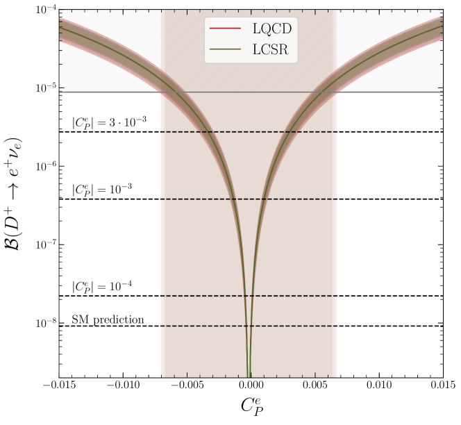
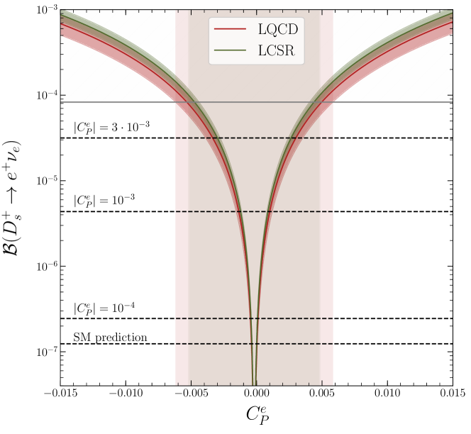
Figure 15: $\mathcal{B}(D_{(s)}^{+}\to e^{+}\nu_{e})$ as functions of $C^{e}_{P}$. The grey regions indicate experimentally excluded regions, while the red and green ones show the allowed values for $C^{e}_{P}$.

Now that we have constraints on the pseudoscalar NP coefficients and determinations of the CKM elements at our disposal, we may combine them to make predictions for the following leptonic branching fractions that have yet to be measured:

$$\mathcal{B}(D^{+}\to e^{+}\nu_{e}),\hskip 28.45274pt\mathcal{B}(D_{s}^{+}\to e^{+}\nu_{e}).$$ (60)

In the SM, these decays are strongly helicity suppressed, as indicated by the smallness of the corresponding SM predictions in Table 1. However, this suppression may be lifted by new pseudoscalar interactions. This is shown in Fig. 15. Here, the branching fractions $\mathcal{B}(D^{+}\to e^{+}\nu_{e})$ and $\mathcal{B}(D_{s}^{+}\to e^{+}\nu_{e})$ are plotted as a function of the coefficient $C^{e}_{P}$. The labels “LQCD” and “LCSR” refer to the form-factor information used to determine the relevant CKM elements in the presence of pseudoscalar NP, given in Eqs. (56–59). The grey regions indicate the experimental upper bounds on the branching fractions. In order to illustrate the sensitivity of the branching fractions to the absolute value of $C^{e}_{P}$, the SM prediction and three predictions for different values of $|C^{e}_{P}|$ are shown in each plot. We see that even a small value for $|C^{e}_{P}|$ has a potentially large effect on the branching fraction, which is a direct consequence of the pseudoscalar NP contributions lifting the helicity suppression in these decays.

At the same time, the obtained constraints on the NP coefficients allow us to predict the branching fractions discussed here in the context of different scenarios related to LFU violation. Let us consider the following scenarios:

• $C^{e}_{P}=C^{\mu}_{P}$. This correlation is indicated by the dashed-dotted lines in Figs. 11 (right) and 12 (right).

• $C^{e}_{P}=(m_{e}/m_{\mu})C^{\mu}_{P}$. This correlation arises, for instance, in the context of a type II Two-Higgs-Doublet model.

• $C^{e}_{P}\gg C^{\mu}_{P}$. We probe the impact of $C^{e}_{P}=10C^{\mu}_{P}$ on the relevant branching fractions.

• $C^{e}_{P}\ll C^{\mu}_{P}$. Similar to the previous scenario, but focusing on the effect of setting $C^{e}_{P}=10^{-1}C^{\mu}_{P}$ for the corresponding branching fractions.

We use the obtained constraints on $C^{\mu}_{P}$, given in Table 4, and relate them to $C^{e}_{P}$ in each scenario accordingly. Subsequently, we use the corresponding values for the CKM elements, given in Table 5, and apply the results to Eq. (15) to obtain a theoretical prediction for the branching fractions $\mathcal{B}(D^{+}\to e^{+}\nu_{e})$ and $\mathcal{B}(D_{s}^{+}\to e^{+}\nu_{e})$ in each of the scenarios. In Figs. 16 and 17, we compare our predictions to the corresponding SM predictions, where $C^{e}_{P}=C^{\mu}_{P}=0$. For the SM prediction, the $|V_{cd(s)}|$ values obtained from unitarity were used. The determination of the relevant CKM elements using LQCD or LCSR form-factor information is indicated by the red and green colours of the bars, respectively. Furthermore, the grey regions indicate the values that are currently already excluded by experiment.

It is interesting to see that in the case $C^{e}_{P}=C^{\mu}_{P}$ in Fig. 16, our predictions for $\mathcal{B}(D^{+}\to e^{+}\nu_{e})$ are very close to the experimental upper limit. For $\mathcal{B}(D_{s}^{+}\to e^{+}\nu_{e})$ illustrated in Fig. 17, our predictions using either LQCD or LCSR based form-factor calculations differ substantially, underlining the importance of precise lattice information on the semileptonic form factors. An observation of spectacularly enhanced $D_{(s)}^{+}\to e^{+}\nu_{e}$ modes close to the current experimental limits would be an unambiguous signal of physics beyond the SM.

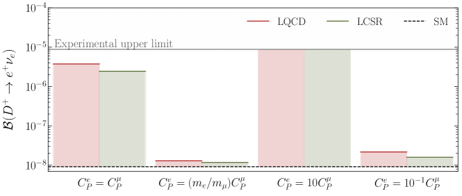
Figure 16: Predictions of $\mathcal{B}(D^{+}\to e^{+}\nu_{e})$ for the scenarios discussed in the text. The red and green bands indicate the LQCD and LCSR form-factor information used. The grey line is the experimental upper limit, while the dashed line is the SM prediction.

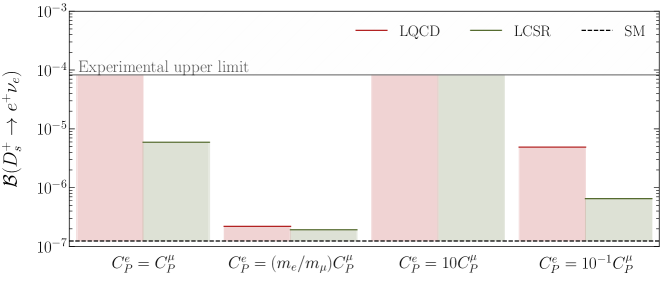
Figure 17: Predictions of $\mathcal{B}(D_{s}^{+}\to e^{+}\nu_{e})$ for the scenarios discussed in the text. The red and green bands indicate the LQCD and LCSR form-factor information used. The grey line is the experimental upper limit, while the dashed line is the SM prediction.

7 Conclusions

We have presented a comprehensive analysis of (semi)-leptonic $D_{(s)}$-meson decays to constrain possible effects of physics from beyond the SM arising from new (pseudo)-scalar, vector and tensor operators, allowing also for violations of LFU. The central role is played by various ratios of decay rates that are independent of the CKM matrix elements $|V_{cd}|$ and $|V_{cs}|$. In the case of leptonic decays, the decay constants cancel there and in the case of combinations of leptonic and semileptonic decays, ratios of non-perturbative hadronic parameters arise that are usually more precise than the individual parameters.

We obtain a picture in agreement with the SM, including a few deviations at the $1\,\sigma$ level. Following our strategy, we may also determine $|V_{cd}|$ and $|V_{cs}|$ from the (semi)-leptonic decays in the presence of NP contributions. The corresponding results are fully consistent with values arising from the unitarity of the CKM matrix and the Wolfenstein parameterization that do not involve any experimental input from the charm system. We have identified various form factors with interesting potential for future improvement through lattice QCD calculations.

The leptonic $D_{(s)}^{+}\to e^{+}\nu_{e}$ decays are hugely helicity suppressed in the SM. However, this suppression may be lifted through new pseudoscalar interactions. Using the constraints following from the interplay between leptonic $D_{(s)}$ decays with muon or tau leptons in the final state and $D\to V\bar{\ell}\nu_{\ell}$ decays, we illustrate that the branching ratio for $D_{(s)}^{+}\to e^{+}\nu_{e}$ may be hugely enhanced and could enter the regime close to the current experimental upper bounds. A future observation of these modes would be an unambiguous signal of NP effects.

We look forward to obtaining stronger constraints on possible violations of LFU in the charged-current interactions in $D_{(s)}$ decays in the high-precision era of quark-flavour physics which is ahead of us.

Appendix A Form Factors

A.1 $D\to P$

The form factors for $D\to P$ decays in the helicity basis are defined as follows [25]:

where $\lambda_{P}(q^{2})=[(M_{D_{(s)}}-m_{P})^{2}-q^{2}][(M_{D_{(s)}}+m_{P})^{2}-q^{2}]$. For our calculations, we adopt the $z$-series parametrization from Ref. [38]. For the $D\to\pi$ case, the scalar and vector form factors are given by

$$f^{D\to\pi}_{+}(q^{2})=\frac{f^{D\to\pi}(0)+c^{D\to\pi}_{+}(z-z_{0})(1+\frac{1}{2}(z+z_{0}))}{1-P_{V}q^{2}},$$ (62)

$$f^{D\to\pi}_{0}(q^{2})=\frac{f^{D\to\pi}(0)+c^{D\to\pi}_{0}(z-z_{0})(1+\frac{1}{2}(z+z_{0}))}{1-P_{S}q^{2}},$$ (63)

where $z_{0}=z(0,t_{0}^{\pi})$. In the case of $D\rightarrow K$ transitions, the scalar and vector form factors are parametrized as

$$f^{D\to K}_{+}(q^{2})=\frac{f^{D\to K}(0)+c^{D\to K}_{+}(z-z_{0})(1+\frac{1}{2}(z+z_{0}))}{1-q^{2}/M^{2}_{D_{s}^{*}}},$$ (64)

$$f^{D\to K}_{0}(q^{2})=f^{D\to K}(0)+c^{D\to K}_{0}(z-z_{0})\Big{(}1+\frac{1}{2}(z+z_{0})\Big{)},$$ (65)

where $z_{0}=z(0,t_{0}^{K})$. The fit parameters are listed in Table 6.

Decay	$f(0)$	$c_{+}$	$P_{V}$ (GeV)-2	$c_{0}$	$P_{S}$ (GeV)-2
$D\rightarrow\pi$	0.6117 (354)	-1.985 (347)	0.1314 (127)	-1.188 (256)	0.0342 (122)
$D\rightarrow K$	0.7647 (308)	-0.066 (333)	-	-2.084 (283)	-

Table 6: Fit parameters for $f_{0}$, $f_{+}$ in the $z$-series expansion [38].

For the tensor form factor, we use the lattice calculation of Ref. [41]. Here, $f_{T}$ is parametrized in the following way:

$$f^{D\to\pi}_{T}(q^{2})=\frac{f^{D\to\pi}_{T}(0)+c^{D\to\pi}_{T}(z-z_{0})(1+\frac{1}{2}(z+z_{0}))}{1-P^{D\to\pi}_{T}q^{2}},$$ (66)

$$f^{D\to K}_{T}(q^{2})=\frac{f^{D\to K}_{T}(0)+c^{D\to K}_{T}(z-z_{0})(1+\frac{1}{2}(z+z_{0}))}{1-P^{D\to K}_{T}q^{2}}.$$ (67)

The fit parameters are given in Table 7.

Decay	$f_{T}(0)$	$c_{T}$	$P_{T}$ (GeV)-2
$D\rightarrow\pi$	0.5063 (786)	-1.10 (1.03)	0.1461 (681)
$D\rightarrow K$	0.6871 (542)	-2.86 (1.46)	0.0854 (671)

Table 7: Fit parameters for $f_{T}$ in the $z$-series expansion [41].

A.2 $D\to V$

The non-zero form factors for $D\to V$ decays in the helicity basis are defined as follows [25]:

$$H^{V}_{V,\pm}=(M_{D}+m_{V})A_{1}(q^{2})\mp\frac{\sqrt{\lambda_{V}(q^{2})}}{M_{D}+m_{V}}V(q^{2}),$$ (68a)

$$H^{V}_{V,0}=\frac{M_{D}+m_{V}}{2M_{V}\sqrt{q^{2}}}\big{[}-(M^{2}_{D}-M_{V}^{2}-q^{2})A_{1}(q^{2})+\frac{\lambda_{V}(q^{2})}{(M_{D}+m_{V})^{2}}A_{2}(q^{2})\big{]},$$ (68b)

$$H^{V}_{V,t}=\sqrt{\frac{\lambda_{V}(q^{2})}{q^{2}}}A_{0}(q^{2}),$$ (68c)

$$H^{V}_{P}=-\frac{\sqrt{\lambda_{V}(q^{2})}}{m_{c}+m_{q}}A_{0}(q^{2}),$$ (68d)

$$H^{V}_{T,\pm}=\frac{1}{\sqrt{q^{2}}}\Big{[}\pm(M^{2}_{D}-m_{V}^{2})T_{2}(q^{2})+\sqrt{\lambda_{V}(q^{2})}T_{1}(q^{2})\Big{]},$$ (68e)

$$H^{V}_{T,0}=\frac{1}{2m_{V}}\big{[}-(M^{2}_{D}+3m^{2}_{V}-q^{2})T_{2}(q^{2})+\frac{\lambda_{V}(q^{2})}{M_{D}^{2}-m_{V}^{2}}T_{3}(q^{2})\big{]},$$ (68f)

where $\lambda_{V}(q^{2})=[(M_{D}-m_{V})^{2}-q^{2}][(M_{D}+m_{V})^{2}-q^{2}]$. We use the lattice determination of the $D\to\rho$ and $D\to K^{*}$ semileptonic form factors from Ref. [42]. The $q^{2}$ dependence is obtained through a single-pole parametrization:

$$V(q^{2})=\frac{V(0)}{1-q^{2}/m^{2}_{1^{-}}},\hskip 14.22636ptA_{0}(q^{2})=\frac{A_{0}(0)}{1-q^{2}/m^{2}_{0^{-}}},\hskip 14.22636ptA_{i}(q^{2})=\frac{A_{i}(0)}{1-q^{2}/m^{2}_{1^{+}}},$$ (69)

where $i=1,2,3$ and $m_{J^{P}}$ denotes the mass of the meson with spin $J$ and parity $P$ corresponding to the relevant quark transition, i.e., $c\bar{d}$ for $D\to\rho$ and $c\bar{s}$ for $D\to K^{*}$. The values for the parameters are given in Table 8. The masses are listed in units of the inverse lattice spacing, which is given by $a^{-1}=(2.73\pm 0.05)$ GeV. The form factor $A_{3}$ is related to the form factors $A_{1}$ and $A_{2}$ in the following way:

$$A_{3}(q^{2})=\frac{M_{D}+m_{V}}{2m_{V}}A_{1}(q^{2})-\frac{M_{D}-m_{V}}{2m_{V}}A_{2}(q^{2}).$$ (70)

Decay	Form Factor	$F(0)$	$m_{J^{P}}[a^{-1}]$
$D\rightarrow\rho$	$A_{0}$	$0.70^{+0.05}_{-0.12}$	$m^{c\bar{d}}_{0^{-}}=0.60^{+0.07}_{-0.05}$
	$A_{1}$	$0.63^{+0.06}_{-0.09}$	$m^{c\bar{d}}_{1^{+}}=1.1^{+0.3}_{-0.2}$
	$A_{2}$	$0.51^{+0.10}_{-0.15}$	$m^{c\bar{d}}_{1^{+}}=0.44^{+0.09}_{-0.05}$
	$V$	$0.95^{+0.29}_{-0.14}$	$m^{c\bar{d}}_{1^{-}}=0.91^{+0.36}_{-0.18}$
$D\rightarrow K^{*}$	$A_{0}$	$0.75^{+0.05}_{-0.11}$	$m^{c\bar{s}}_{0^{-}}=0.59^{+0.06}_{-0.05}$
	$A_{1}$	$0.70^{+0.07}_{-0.10}$	$m^{c\bar{s}}_{1^{+}}=1.1^{+0.3}_{-0.2}$
	$A_{2}$	$0.66^{+0.10}_{-0.15}$	$m^{c\bar{s}}_{1^{+}}=0.46^{+0.16}_{-0.07}$
	$V$	$1.01^{+0.30}_{-0.13}$	$m^{c\bar{s}}_{1^{-}}=0.85^{+0.24}_{-0.15}$

Table 8: LQCD fit parameters for the $D\to\rho$ and $D\to K^{*}$ form factors, taken from Ref. [42].

We complement the lattice calculation with the LCSR calculation of Ref. [43]. This work dates back to 2006, but there exists a more recent determination of the $D\to\rho$ form factors [45]. In this analysis, the massless lepton limit is taken, neglecting the form factor $A_{0}$. In our study, we investigate the difference between different lepton flavours, therefore requiring information on $A_{0}$. We therefore utilize the form-factor information of Ref. [43], where the following double-pole parametrization was adopted:

$$F^{i}(q^{2})=\frac{F^{i}(0)}{1-a_{F^{i}}q^{2}/M_{D}^{2}+b_{F^{i}}(q^{2}/M_{D_{(s)}}^{2})^{2}},$$ (71)

with $F^{i}$ denoting any of the form factors $A_{1}$, $A_{2}$, $A_{3}$ or $V$. Here, a different convention is used: instead of the set $\{A_{0},A_{1},A_{2}\}$, the hadronic matrix elements are parametrized by the set $\{A_{1},A_{2},A_{3}\}$. The relation between the different conventions is given by the following relation [46]:

$$A_{0}(q^{2})=\frac{1}{2m_{V}}\Big{[}(M_{D}+m_{V})A_{1}(q^{2})-(M_{D}-m_{V})A_{2}(q^{2})-\frac{q^{2}}{M_{D}+m_{V}}A_{3}(q^{2})\Big{]}.$$ (72)

The results from LCSR for the fit parameters for $D\to\rho$ and $D\to K^{*}$ transitions are listed in Table 9.

Decay	Form Factor	$F(0)$	$a_{F}$	$b_{F}$
$D\rightarrow\rho$	$A_{1}$	$0.590^{+0.031}_{-0.029}$	$0.44^{-0.04}_{+0.05}$	$0.20^{-0.03}_{+0.10}$
	$A_{2}$	$0.528^{+0.036}_{-0.031}$	$0.91^{+0.07}_{-0.13}$	$-1.01^{+0.22}_{-0.41}$
	$A_{3}$	$-0.528^{+0.031}_{-0.026}$	$0.91^{-0.13}_{+0.07}$	$-1.01^{-0.41}_{+0.22}$
	$V$	$0.735^{+0.032}_{-0.025}$	$0.48^{-0.11}_{+0.21}$	$2.25^{-0.21}_{+0.61}$
$D\rightarrow K^{*}$	$A_{1}$	$0.601^{+0.030}_{-0.029}$	$0.51^{-0.02}_{+0.02}$	$0.04^{+0.01}_{-0.01}$
	$A_{2}$	$0.541^{+0.038}_{-0.033}$	$0.91^{+0.05}_{-0.10}$	$-0.68^{+0.12}_{-0.21}$
	$A_{3}$	$-0.541^{+0.033}_{-0.038}$	$0.91^{-0.10}_{+0.05}$	$-0.68^{-0.21}_{+0.12}$
	$V$	$0.796^{+0.032}_{-0.027}$	$0.60^{-0.07}_{+0.13}$	$1.53^{-0.13}_{+0.30}$

Table 9: LCSR fit parameters for the $D\to\rho$ and $D\to K^{*}$ form factors, taken from Ref. [43].

References

- [1] A. J. Buras, D. Buttazzo, J. Girrbach-Noe, and R. Knegjens, Can we reach the Zeptouniverse with rare and decays?, JHEP 11 (2014) 121. arXiv: 1408.0728 [hep-ph].
- [2] Y. Li and C.–D. Lü, Recent Anomalies in B Physics, Sci. Bull. 63 (2018) 267-269. arXiv: 1808.02990 [hep-ph].
- [3] S. Bifani, S. Descotes-Genon, A. Romero Vidal and M.–H. Schune, Review of Lepton Universality tests in decays, J. Phys. G46 (2019) 2, 023001. arXiv: 1809.06229 [hep-ex].
- [4] Y. S. Amhis et al. (Heavy Flavor Averaging Group), Averages of -hadron, -hadron, and -lepton properties as of 2018, (2019). arXiv: 1909.12524 [hep-ex].
- [5] R. Aaij et al. (LHCb Collaboration), Search for lepton-universality violation in decays, Phys. Rev. Lett. 122 (2019) 19, 191801. arXiv: 1903.09252 [hep-ex].
- [6] R. Aaij et al. (LHCb Collaboration), Test of lepton universality with decays, JHEP 08 (2017) 055. arXiv: 1705.05802 [hep-ex].
- [7] D. Bečirević and O. Sumensari, A leptoquark model to accommodate and , JHEP 08 (2017) 104. arXiv: 1704.05835 [hep-ph].
- [8] L. Calibbi, A. Crivellin and T. Li, Model of vector leptoquarks in view of the -physics anomalies, Phys. Rev. D98 (2018) 11, 115002. arXiv: 1709.00692 [hep-ph].
- [9] M. Blanke and A. Crivellin, Meson Anomalies in a Pati-Salam Model within the Randall-Sundrum Background, Phys. Rev. Lett. 121 (2018) 1, 011801 arXiv: 1801.07256 [hep-ph].
- [10] A. Crivellin, C. Greub, D. Müller and F. Saturnino, Importance of Loop Effects in Explaining the Accumulated Evidence for New Physics in B Decays with a Vector Leptoquark, Phys. Rev. Lett. 122 (2019) 1, 011805. arXiv: 1807.02068 [hep-ph].
- [11] C. Cornella, J. Fuentes-Martin and G. Isidori, Revisiting the vector leptoquark explanation of the B-physics anomalies, JHEP 07 (2019) 168. arXiv: 1903.11517 [hep-ph].
- [12] O. Popov, M. A. Schmidt and G. White, as a single leptoquark solution to and , Phys. Rev. D100 (2019) 3, 035028. arXiv: 1905.06339 [hep-ph].
- [13] L. Bian, H. M. Lee and C. B. Park, -meson anomalies and Higgs physics in flavored model, Eur. Phys. J. C78 (2018) 4, 306. arXiv: 1711.08930 [hep-ph].
- [14] B. C. Allanach, T. Corbett, M. J. Dolan and T. You, Hadron collider sensitivity to fat flavourful s for , JHEP 03 (2019) 137. arXiv: 1810.02166 [hep-ph].
- [15] L. Calibbi, A. Crivellin, F. Kirk, C. A. Manzari and L. Vernazza, models with less-minimal flavour violation, (2019). arXiv: 1910.00014 [hep-ph].
- [16] C. Niehoff, P. Stangl and D. M. Straub, Violation of lepton flavour universality in composite Higgs models, Phys. Lett. B747 (2015) 182-186. arXiv: 1503.03865 [hep-ph].
- [17] S. Iguro and K. Tobe, in a general two Higgs doublet model, Nucl. Phys. B925 (2017) 560-606. arXiv: 1708.06176 [hep-ph].
- [18] A. Crivellin, D. Müller and C. Wiegand, transitions in two-Higgs-doublet models, JHEP 06 (2019) 119. arXiv: 1903.10440 [hep-ph].
- [19] R. Bause, M. Golz, G. Hiller and A. Tayduganov, The New Physics Reach of Null Tests with and Decays. arXiv: 1909.11108 [hep-ph].
- [20] A. Crivellin, G. D’Ambrosio, M. Hoferichter and L. C. Tunstall, Violation of lepton flavor and lepton flavor universality in rare kaon decays, Phys. Rev. D93 (2016) 7, 074038. arXiv: 1601.00970 [hep-ph].
- [21] S. Fajfer, I. Nisandzic and U. Rojec, Discerning new physics in charm meson leptonic and semileptonic decays, Phys. Rev. D91 (2015) 9, 094009. arXiv: 1502.07488 [hep-ph].
- [22] G. Banelli, R. Fleischer, R. Jaarsma and G. Tetlalmatzi-Xolocotzi, Decoding (Pseudo)-Scalar Operators in Leptonic and Semileptonic Decays, Eur. Phys. J. C78 (2018) 11, 911. arXiv: 1809.09051 [hep-ph].
- [23] G. Banelli, R. Fleischer, R. Jaarsma and G. Tetlalmatzi-Xolocotzi, Probing Lepton Universality with (Semi)-Leptonic B decays, SciPost Phys. Proc. 1 (2019) 013. arXiv:1812.05200 [hep-ph].
- [24] Tanaka, M. and Watanabe, R., New physics in the weak interaction of , Phys. Rev. D87 (2013) 3, 034028. arXiv: 1212.1878 [hep-ph] .
- [25] Y. Sakaki, M. Tanaka, A. Tayduganov and R. Watanabe, Testing leptoquark models in , Phys. Rev. D88 (2013) 9, 094012. arXiv: 1309.0301 [hep-ph].
- [26] L. Riggio, G. Salerno and S. Simula, Extraction of and from experimental decay rates using lattice QCD form factors, Eur. Phys. J. C78 (2018) 6, 501. arXiv: 1706.03657 [hep-lat].
- [27] L. Wolfenstein, Parametrization of the Kobayashi-Maskawa Matrix, Phys. Rev. Lett. 51 (1983) 1945. doi: 10.1103/PhysRevLett.51.1945 .
- [28] A. J. Buras, M. E. Lautenbacher and G. Ostermaier, Waiting for the top quark mass, , mixing and CP asymmetries in B decays, Phys. Rev. D50 (1994) 3433-3446. doi: 10.1103/PhysRevD.50.3433.
- [29] A. J. Buras, Unitarity triangle: 2002 and beyond, 14th Rencontres de Blois on Matter - Anti-matter Asymmetry Chateau de Blois, France, June 17-22, 2002 (2002). eprint: hep-ph/0210291 [hep-ph].
- [30] M. Tanabashi et al. (Particle Data Group), Review of Particle Physics, Phys. Rev. D98 (2018) 3, 030001. doi: 10.1103/PhysRevD.98.030001.
- [31] C. Bouchard, L. Cao and P. Owen, Summary of the 2018 CKM working group on semileptonic and leptonic -hadron decays, 10th International Workshop on the CKM Unitarity Triangle (CKM 2018) Heidelberg, Germany, September 17-21, 2018 (2019). arXiv: 1902.09412 [hep-ex].
- [32] S. Aoki et al. (Flavour Lattice Averaging Group), FLAG Review 2019, (2019). arXiv: 1902.08191 [hep-lat].
- [33] A. G. Akeroyd, Effect of on and , Prog. Theor. Phys. 111 (2004) 295-299. doi: 10.1143/PTP.111.295.
- [34] A. G. Akeroyd and F. Mahmoudi, Constraints on charged Higgs bosons from and , JHEP 04 (2009) 121. arXiv: 0902.2393 [hep-ph].
- [35] A. G. Akeroyd and S. Recksiegel, Large enhancement of and in parity violating SUSY models, Phys. Lett. B554 (2003) 38-44. doi: 10.1016/S0370-2693(02)03293-8.
- [36] M. Ablikim et al. (BESIII Collaboration), Observation of the leptonic decay , Phys. Rev. Lett. 123 (2019) 21, 211802. arXiv: 1908.08877 [hep-ex].
- [37] C. Aubin et al. (Fermilab Lattice, MILC and HPQCD Collaborations), Semileptonic decays of D mesons in three-flavor lattice QCD, Phys. Rev. Lett. 94 (2005) 011601. doi: 10.1103/PhysRevLett.94.011601.
- [38] V. Lubicz, L. Riggio, G. Salerno, S. Simula and C. Tarantino (ETM Collaboration), Scalar and vector form factors of decays with twisted fermions, Phys. Rev. D96 (2017) 5, 054514. arXiv: 1706.03017 [hep-lat].
- [39] M. A. Ivanov, J. G. Körner, J. N. Pandya, P. Santorelli, N. R. Soni and C. T. Tran, Exclusive semileptonic decays of D and Ds mesons in the covariant confining quark model, Front. Phys. (Beijing) 14 (2019) 6, 64401. arXiv: 1904.07740 [hep-ph].
- [40] R. N. Faustov, V. O. Galkin and X. W. Kang, Semileptonic decays of and mesons in the relativistic quark model, (2019). arXiv: 1911.08209 [hep-ph].
- [41] V. Lubicz, L. Riggio, G. Salerno, S. Simula and C. Tarantino (ETM Collaboration), Tensor form factor of and decays with twisted-mass fermions, Phys. Rev. D98 (2018) 1, 014516. arXiv: 1803.04807 [hep-lat].
- [42] K. C. Bowler et al. (UKQCD Collaboration), An ‘improved’ lattice study of semileptonic decays of D mesons, Phys. Rev. D51 (1995) 4905-4923. doi: 10.1103/PhysRevD.51.4905.
- [43] Y.–L. Wu, M. Zhong and Y.–B. Zuo, Transition Form Factors and Decay Rates with Extraction of the CKM parameters , , , Int. J. Mod. Phys. A21 (2004) 6125-6172. doi: 10.1142/S0217751X06033209.
- [44] M. Fael, T. Mannel and K. K. Vos, The Heavy Quark Expansion for Inclusive Semileptonic Charm Decays Revisited, JHEP 12 (2019) 067. arXiv: 1910.05234 [hep-ph].
- [45] H.–B. Fu, X. Yang, R. Lü, L. Zeng, W. Cheng and X.-G. Wu, The transition form factors within the QCD light-cone sum rules and the -meson semileptonic decays and , (2018). arXiv: 1808.06412 [hep-ph].
- [46] W. Y. Wang, Y.–L. Wu and M. Zhong, Heavy to light meson exclusive semileptonic decays in effective field theory of heavy quarks, Phys. Rev. D67 (2003) 014024. doi: 10.1103/PhysRevD.67.014024.