1 Introduction
In many applications in signal or image processing great importance is attached to precise information about the location and order of singularities of signals. In one dimension this corresponds to functions which are smooth apart from pointwise singularities. Many authors discussed this problem when the Fourier coefficients of a periodic function are given, see e.g. [1 , 6 , 7 , 27 , 31 , 34 ] .
Because of their localization properties in the time and frequency domain, wavelet expansions provide a powerful tool for detecting and analyzing point discontinuities in one or more dimensions [17 , 26 ] . The reason is that only very few wavelet coefficients of translates near the location of the singularity are large in magnitude, while all other wavelet coefficients corresponding to translates which are further away from the point discontinuity decay rapidly. A framework for univariate periodic wavelets was investigated by several authors [18 , 28 , 29 , 30 ] and some of these constructions were successfully used for the detection of pointwise singularities of periodic functions [27 ] .
In two dimensions the situation is more complex since not only point singularities can occur but also discontinuities along curves. To deal with these types of singularities, along with many other constructions, the theory of the continuous shearlet transform was developed [5 , 11 , 21 ] and defined as the mapping
f → 𝒮 ℋ ψ f ( a , s , p ) = ⟨ f , ψ a , s , 𝐩 ⟩ → 𝑓 𝒮 subscript ℋ 𝜓 𝑓 𝑎 𝑠 𝑝 𝑓 subscript 𝜓 𝑎 𝑠 𝐩
f\rightarrow\mathcal{SH}_{\psi}f(a,s,p)=\left\langle f,\psi_{a,s,\mathbf{p}}\right\rangle
with scale parameter a > 0 𝑎 0 a>0 s ∈ ℝ 𝑠 ℝ s\in\mathbb{R} 𝐩 ∈ ℝ 2 𝐩 superscript ℝ 2 \mathbf{p}\in\mathbb{R}^{2} ψ a , s , 𝐩 subscript 𝜓 𝑎 𝑠 𝐩
\psi_{a,s,\mathbf{p}} s 𝑠 s T ⊂ ℝ 2 𝑇 superscript ℝ 2 T\subset\mathbb{R}^{2} ∂ T 𝑇 \partial T 𝐩 ∉ ∂ T 𝐩 𝑇 \mathbf{p}\notin\partial T s = s 0 𝑠 subscript 𝑠 0 s=s_{0} ∂ T 𝑇 \partial T 𝐩 𝐩 \mathbf{p}
lim a → 0 + a − N 𝒮 ℋ ψ χ T ( a , s 0 , 𝐩 ) = 0 for all N > 0 . formulae-sequence subscript → 𝑎 superscript 0 superscript 𝑎 𝑁 𝒮 subscript ℋ 𝜓 subscript 𝜒 𝑇 𝑎 subscript 𝑠 0 𝐩 0 for all 𝑁 0 \lim\limits_{a\rightarrow 0^{+}}a^{-N}\mathcal{SH}_{\psi}\chi_{T}(a,s_{0},\mathbf{p})=0\qquad\text{for all}\;N>0. (1)
Otherwise, if 𝐩 ∈ ∂ T 𝐩 𝑇 \mathbf{p}\in\partial T s = s 0 𝑠 subscript 𝑠 0 s=s_{0} ∂ T 𝑇 \partial T 𝐩 𝐩 \mathbf{p}
lim a → 0 + a − 3 / 4 𝒮 ℋ ψ χ T ( a , s 0 , 𝐩 ) = C > 0 . subscript → 𝑎 superscript 0 superscript 𝑎 3 4 𝒮 subscript ℋ 𝜓 subscript 𝜒 𝑇 𝑎 subscript 𝑠 0 𝐩 𝐶 0 \lim\limits_{a\rightarrow 0^{+}}a^{-3/4}\mathcal{SH}_{\psi}\chi_{T}(a,s_{0},\mathbf{p})=C>0. (2)
The results were shown for continuous shearlets, which are compactly supported in the time [22 ] or frequency domain [9 , 12 , 13 , 20 ] .
Based on these theoretical results, practical applications for the detection of edges in images were developed [35 ] .
Therefore, discrete frames of shearlets were constructed by sampling the parameters of the continuous shearlet systems in a suitable way [19 ] . Based on the result for curvelets [4 ] , it was possible to show that discrete shearlet systems are essentially optimal for the sparse approximation of so-called cartoon-like functions [23 ] . This result implies the upper estimate
| ⟨ f , ψ j , ℓ , 𝐤 ⟩ | ≤ C 2 − 3 j / 2 𝑓 subscript 𝜓 𝑗 ℓ 𝐤
𝐶 superscript 2 3 𝑗 2 \left\lvert\left\langle f,\psi_{j,\ell,\mathbf{k}}\right\rangle\right\rvert\leq C\,2^{-3j/2} (3)
for some constant C > 0 𝐶 0 C>0 j 𝑗 j [14 ] , the authors showed the existence of a lower estimate | ⟨ χ T , ψ j , ℓ , 𝐤 ℓ ⟩ | ≥ C 2 − 3 j / 2 subscript 𝜒 𝑇 subscript 𝜓 𝑗 ℓ subscript 𝐤 ℓ
𝐶 superscript 2 3 𝑗 2 \left\lvert\left\langle\chi_{T},\psi_{j,\ell,\mathbf{k}_{\ell}}\right\rangle\right\rvert\geq C\,2^{-3j/2} Eq. 1 Eq. 2
The framework of multivariate periodic wavelets was developed for example in [8 , 25 ] . In [3 , 24 ] the corresponding wavelet functions were trigonometric polynomials of Dirichlet and de la Vallée Poussin-type, which can be well localized in the time and frequency domain. The construction allows for fast decomposition algorithms [2 ] with many different dilation matrices on each scale, including shearing. This gives rise to directional decompositions of the frequency domain similar to the tilling of the frequency plane in the case of discrete shearlet systems [4 , 14 ] .
In this paper we use the latter construction to prove two main theorems which provide upper and lower bounds similar to [14 ] , but this time for a discrete system of periodic de la Vallée Poussin-type wavelets that are trigonometric polynomials. The upper estimate in Theorem 3.1 Eq. 3 Theorem 3.2 [14 ] and implies that the constructed trigonometric polynomial shearlets in this paper are able to detect step discontinuities along boundary curves of periodic functions.
The paper is organized as follows. We start with the construction of a special case of directional de la Vallée Poussin wavelets in Section 2 Section 3 Section 4 Section 5 Section 6
2 Trigonometric polynomial shearlets
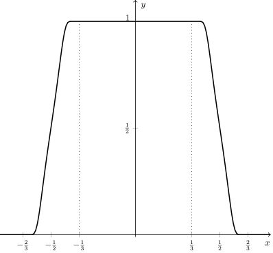
If a nonnegative and even function g : ℝ → ℝ : 𝑔 → ℝ ℝ g:\mathbb{R}\rightarrow\mathbb{R} supp g = ( − 2 3 , 2 3 ) supp 𝑔 2 3 2 3 \mathrm{supp}\,g=\left(-\frac{2}{3},\frac{2}{3}\right)
∑ z ∈ ℤ g ( x + z ) = 1 for all x ∈ ℝ , subscript 𝑧 ℤ 𝑔 𝑥 𝑧 1 for all 𝑥 ℝ \sum\limits_{z\in\mathbb{Z}}g(x+z)=1\;\;\text{for all}\;\;x\in\mathbb{R},
we call it window function and write g ∈ 𝒲 𝑔 𝒲 g\in\mathcal{W} g 𝑔 g q 𝑞 q g ∈ 𝒲 q 𝑔 superscript 𝒲 𝑞 g\in\mathcal{W}^{q} g ( x ) = 1 𝑔 𝑥 1 g(x)=1 x ∈ ( − 1 3 , 1 3 ) 𝑥 1 3 1 3 x\in\left(-\frac{1}{3},\frac{1}{3}\right) g 𝑔 g x ∈ ( − 2 3 , − 1 3 ] 𝑥 2 3 1 3 x\in\left(-\frac{2}{3},-\frac{1}{3}\right] x ∈ [ 1 3 , 2 3 ) 𝑥 1 3 2 3 x\in\left[\frac{1}{3},\frac{2}{3}\right) g ~ : ℝ → ℝ : ~ 𝑔 → ℝ ℝ \widetilde{g}:\mathbb{R}\rightarrow\mathbb{R} g ~ ( x ) : = g ( x 2 ) − g ( x ) \widetilde{g}(x)\mathrel{\mathop{:}}=g\left(\frac{x}{2}\right)-g(x)
As an example of a window function we consider
r ( x ) = { e − b / x 2 , for x > 0 , 0 , for x ≤ 0 , 𝑟 𝑥 cases superscript e 𝑏 superscript 𝑥 2 for 𝑥 0 0 for 𝑥 0 r(x)=\begin{cases}\mathrm{e}^{-b/x^{2}},&\text{for }x>0,\\
0,&\text{for }x\leq 0,\end{cases}
where b > 0 𝑏 0 b>0 s ( x ) = r ( 2 3 + x ) r ( 2 3 − x ) 𝑠 𝑥 𝑟 2 3 𝑥 𝑟 2 3 𝑥 s(x)=r\left(\frac{2}{3}+x\right)\,r\left(\frac{2}{3}-x\right)
g b ( x ) = s ( x ) ∑ k ∈ ℤ s ( x + k ) subscript 𝑔 𝑏 𝑥 𝑠 𝑥 subscript 𝑘 ℤ 𝑠 𝑥 𝑘 g_{b}(x)=\frac{s(x)}{\sum\limits_{k\in\mathbb{Z}}s(x+k)} (4)
we have g b ∈ 𝒲 ∞ subscript 𝑔 𝑏 superscript 𝒲 g_{b}\in\mathcal{W}^{\infty} Figure 1 b = 0.025 𝑏 0.025 b=0.025
We denote two-dimensional vectors by 𝐱 = ( x 1 , x 2 ) T 𝐱 superscript subscript 𝑥 1 subscript 𝑥 2 T \mathbf{x}=(x_{1},x_{2})^{\mathrm{T}} 𝐱 T 𝐲 : = x 1 y 1 + x 2 y 2 \mathbf{x}^{\mathrm{T}}\mathbf{y}\mathrel{\mathop{:}}=x_{1}\,y_{1}+x_{2}\,y_{2} | 𝐱 | 2 : = 𝐱 T 𝐱 \left\lvert\mathbf{x}\right\rvert_{2}\mathrel{\mathop{:}}=\sqrt{\mathbf{x}^{\mathrm{T}}\mathbf{x}} C ( A ) 𝐶 𝐴 C(A) A ⊆ ℝ 2 𝐴 superscript ℝ 2 A\subseteq\mathbb{R}^{2} ∥ f ∥ A , ∞ : = ∥ f ∥ C ( A ) : = sup 𝐱 ∈ A | f ( 𝐱 ) | \left\lVert f\right\rVert_{A,\infty}\mathrel{\mathop{:}}=\left\lVert f\right\rVert_{C(A)}\mathrel{\mathop{:}}=\sup\limits_{\mathbf{x}\in A}\left\lvert f(\mathbf{x})\right\rvert 𝐱 ∈ ℝ 2 𝐱 superscript ℝ 2 \mathbf{x}\in\mathbb{R}^{2} 𝐫 = ( r 1 , r 2 ) T ∈ ℕ 0 2 𝐫 superscript subscript 𝑟 1 subscript 𝑟 2 T superscript subscript ℕ 0 2 \mathbf{r}=(r_{1},r_{2})^{\mathrm{T}}\in\mathbb{N}_{0}^{2} f 𝑓 f
∂ 𝐫 f ( 𝐱 ) : = ∂ r 1 + r 2 ∂ x 1 r 1 ∂ x 2 r 2 f ( 𝐱 ) \partial^{\mathbf{r}}f(\mathbf{x})\mathrel{\mathop{:}}=\frac{\partial^{r_{1}+r_{2}}}{\partial x_{1}^{r_{1}}\partial x_{2}^{r_{2}}}f(\mathbf{x})
and the space of all q 𝑞 q
C 0 q ( A ) : = { f : A → ℝ : ∂ 𝐫 f ∈ C ( A ) for all 𝐫 ∈ ℕ 0 2 with r 1 + r 2 ≤ q , | supp f | < ∞ } C^{q}_{0}(A)\mathrel{\mathop{:}}=\left\{f:A\rightarrow\mathbb{R}:\partial^{\mathbf{r}}f\in C(A)\;\text{for all}\;\mathbf{r}\in\mathbb{N}_{0}^{2}\;\text{with}\;r_{1}+r_{2}\leq q,\,\left\lvert\mathrm{supp}\,f\right\rvert<\infty\right\}
with the norm
∥ f ∥ C q : = ∥ f ∥ C q ( A ) : = sup r 1 + r 2 ≤ q sup 𝐱 ∈ A | ∂ 𝐫 f ( 𝐱 ) | . \left\lVert f\right\rVert_{C^{q}}\mathrel{\mathop{:}}=\left\lVert f\right\rVert_{C^{q}(A)}\mathrel{\mathop{:}}=\sup\limits_{r_{1}+r_{2}\leq q}\,\sup\limits_{\mathbf{x}\in A}\left\lvert\partial^{\mathbf{r}}f(\mathbf{x})\right\rvert.
For i ∈ { h , v } 𝑖 h v i\in\{\mathrm{h},\mathrm{v}\} Ψ ( i ) : ℝ 2 → ℝ : superscript Ψ 𝑖 → superscript ℝ 2 ℝ \Psi^{(i)}:\mathbb{R}^{2}\rightarrow\mathbb{R}
Ψ ( h ) ( 𝐱 ) : = g ~ ( x 1 ) g ( x 2 ) , Ψ ( v ) ( 𝐱 ) : = g ( x 1 ) g ~ ( x 2 ) . \Psi^{(\mathrm{h})}(\mathbf{x})\mathrel{\mathop{:}}=\widetilde{g}(x_{1})\,g(x_{2}),\qquad\qquad\Psi^{(\mathrm{v})}(\mathbf{x})\mathrel{\mathop{:}}=g(x_{1})\,\widetilde{g}(x_{2}).
We remark that for g ∈ 𝒲 q 𝑔 superscript 𝒲 𝑞 g\in\mathcal{W}^{q} Ψ ( i ) ∈ C 0 q ( ℝ 2 ) superscript Ψ 𝑖 subscript superscript 𝐶 𝑞 0 superscript ℝ 2 \Psi^{(i)}\in C^{q}_{0}(\mathbb{R}^{2}) Ψ ( i ) ∈ 𝒲 2 q superscript Ψ 𝑖 superscript subscript 𝒲 2 𝑞 \Psi^{(i)}\in\mathcal{W}_{2}^{q} g ∈ 𝒲 𝑔 𝒲 g\in\mathcal{W}
supp Ψ ( h ) = ( ( − 4 3 , − 1 3 ) ∪ ( 1 3 , 4 3 ) ) × ( − 2 3 , 2 3 ) , supp superscript Ψ h 4 3 1 3 1 3 4 3 2 3 2 3 \displaystyle\mathrm{supp}\,\Psi^{(\mathrm{h})}=\left(\left(-\frac{4}{3},-\frac{1}{3}\right)\cup\left(\frac{1}{3},\frac{4}{3}\right)\right)\times\left(-\frac{2}{3},\frac{2}{3}\right),
supp Ψ ( v ) = ( − 2 3 , 2 3 ) × ( ( − 4 3 , − 1 3 ) ∪ ( 1 3 , 4 3 ) ) . supp superscript Ψ v 2 3 2 3 4 3 1 3 1 3 4 3 \displaystyle\mathrm{supp}\,\Psi^{(\mathrm{v})}=\left(-\frac{2}{3},\frac{2}{3}\right)\times\left(\left(-\frac{4}{3},-\frac{1}{3}\right)\cup\left(\frac{1}{3},\frac{4}{3}\right)\right).
For even j ∈ ℕ 0 𝑗 subscript ℕ 0 j\in\mathbb{N}_{0} ℓ ∈ ℤ ℓ ℤ \ell\in\mathbb{Z} | ℓ | ≤ 2 j / 2 ℓ superscript 2 𝑗 2 \lvert\ell\rvert\leq 2^{j/2}
𝐍 j , ℓ ( h ) : = ( 2 j ℓ 2 j / 2 0 2 j / 2 ) , 𝐍 j , ℓ ( v ) : = ( 2 j / 2 0 ℓ 2 j / 2 2 j ) \mathbf{N}_{j,\ell}^{(\mathrm{h})}\mathrel{\mathop{:}}=\begin{pmatrix}2^{j}&\ell\,2^{j/2}\\
0&2^{j/2}\end{pmatrix},\qquad\qquad\;\mathbf{N}_{j,\ell}^{(\mathrm{v})}\mathrel{\mathop{:}}=\begin{pmatrix}2^{j/2}&0\\
\ell\,2^{j/2}&2^{j}\end{pmatrix} (5)
and the corresponding discrete angles
θ j , ℓ ( h ) : = arctan ( ℓ 2 − j / 2 ) , θ j , ℓ ( v ) : = arccot ( ℓ 2 − j / 2 ) . \theta_{j,\ell}^{(\mathrm{h})}\mathrel{\mathop{:}}=\arctan\left(\ell\,2^{-j/2}\right),\qquad\qquad\theta_{j,\ell}^{(\mathrm{v})}\mathrel{\mathop{:}}=\mathrm{arccot}\left(\ell\,2^{-j/2}\right).
Note that these matrices occur in the construction of discrete shearlet systems, for example in [14 , 23 ] . Based on this, we introduce the notation
Ψ j , ℓ ( i ) ( ⋅ ) : = Ψ ( i ) ( ( 𝐍 j , ℓ ( i ) ) − T ⋅ ) \Psi^{(i)}_{j,\ell}(\cdot)\mathrel{\mathop{:}}=\Psi^{(i)}\left(\left(\mathbf{N}_{j,\ell}^{(i)}\right)^{-\mathrm{T}}\cdot\right) (6)
and, since det 𝐍 j , ℓ ( i ) = 2 3 j / 2 superscript subscript 𝐍 𝑗 ℓ
𝑖 superscript 2 3 𝑗 2 \det\mathbf{N}_{j,\ell}^{(i)}=2^{3j/2}
| supp Ψ j , ℓ ( i ) | = | supp Ψ ( i ) | det 𝐍 j , ℓ ( i ) = 8 3 2 3 j / 2 . supp subscript superscript Ψ 𝑖 𝑗 ℓ
supp superscript Ψ 𝑖 superscript subscript 𝐍 𝑗 ℓ
𝑖 8 3 superscript 2 3 𝑗 2 \left\lvert\mathrm{supp}\,\Psi^{(i)}_{j,\ell}\right\rvert=\left\lvert\mathrm{supp}\,\Psi^{(i)}\right\rvert\det\mathbf{N}_{j,\ell}^{(i)}=\frac{8}{3}\,2^{3j/2}. (7)
Figure 1: Left: The window function g 0.025 ∈ 𝒲 ∞ subscript 𝑔 0.025 superscript 𝒲 g_{0.025}\in\mathcal{W}^{\infty} Eq. 4 supp Ψ 10 , ℓ ( i ) supp superscript subscript Ψ 10 ℓ
𝑖 \mathrm{supp}\,\Psi_{10,\ell}^{(i)} W 10 , ℓ ( i ) superscript subscript 𝑊 10 ℓ
𝑖 W_{10,\ell}^{(i)} ℓ = 5 , 25 ℓ 5 25
\ell=5,25 i ∈ { h , v } 𝑖 h v i\in\{\mathrm{h},\mathrm{v}\} θ 10 , ℓ ( i ) superscript subscript 𝜃 10 ℓ
𝑖 \theta_{10,\ell}^{(i)}
In polar coordinates, we define the sets
W j , ℓ ( h ) : = { ( ρ , θ ) ∈ ℝ × [ − π 2 , π 2 ] : 2 j 3 < | ρ | < 2 j + 1 , θ j , ℓ − 2 ( h ) < θ < θ j , ℓ + 2 ( h ) } , \displaystyle W_{j,\ell}^{(\mathrm{h})}\mathrel{\mathop{:}}=\left\{(\rho,\theta)\in\mathbb{R}\times\left[-\frac{\pi}{2},\frac{\pi}{2}\right]:\frac{2^{j}}{3}<\left\lvert\rho\right\rvert<2^{j+1},\,\theta_{j,\ell-2}^{(\mathrm{h})}<\theta<\theta_{j,\ell+2}^{(\mathrm{h})}\right\},
W j , ℓ ( v ) : = { ( ρ , θ ) ∈ ℝ × [ 0 , π ] : 2 j 3 < | ρ | < 2 j + 1 , θ j , ℓ + 2 ( v ) < θ < θ j , ℓ − 2 ( v ) } \displaystyle W_{j,\ell}^{(\mathrm{v})}\mathrel{\mathop{:}}=\left\{(\rho,\theta)\in\mathbb{R}\times\left[0,\pi\right]:\frac{2^{j}}{3}<\left\lvert\rho\right\rvert<2^{j+1},\,\theta_{j,\ell+2}^{(\mathrm{v})}<\theta<\theta_{j,\ell-2}^{(\mathrm{v})}\right\}
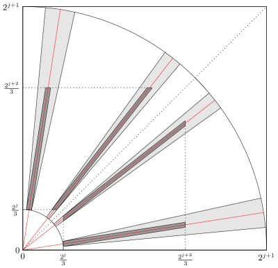
and based on ideas from [23 , Proposition 2.1] we show the following lemma, which is visualized on the right side of Figure 1
Lemma 2.1 .
For even j ≥ 10 𝑗 10 j\geq 10 ℓ ∈ ℤ ℓ ℤ \ell\in\mathbb{Z} | ℓ | ≤ 2 j / 2 ℓ superscript 2 𝑗 2 \left\lvert\ell\right\rvert\leq 2^{j/2} i ∈ { h , v } 𝑖 h v i\in\{\mathrm{h},\mathrm{v}\}
supp Ψ j , ℓ ( i ) ( ρ , θ ) ⊂ W j , ℓ ( i ) . supp superscript subscript Ψ 𝑗 ℓ
𝑖 𝜌 𝜃 superscript subscript 𝑊 𝑗 ℓ
𝑖 \mathrm{supp}\,\Psi_{j,\ell}^{(i)}(\rho,\theta)\subset W_{j,\ell}^{(i)}.
Proof.
We show only the case i = h 𝑖 h i=\mathrm{h} Eq. 6
Ψ j , ℓ ( h ) ( 𝝃 ) = Ψ ( h ) ( ( 𝐍 j , ℓ ( h ) ) − T 𝝃 ) = g ~ ( 2 − j ξ 1 ) g ( 2 − j ξ 1 ( 2 j / 2 ξ 2 ξ 1 − ℓ ) ) superscript subscript Ψ 𝑗 ℓ
h 𝝃 superscript Ψ h superscript superscript subscript 𝐍 𝑗 ℓ
h T 𝝃 ~ 𝑔 superscript 2 𝑗 subscript 𝜉 1 𝑔 superscript 2 𝑗 subscript 𝜉 1 superscript 2 𝑗 2 subscript 𝜉 2 subscript 𝜉 1 ℓ \Psi_{j,\ell}^{(\mathrm{h})}(\boldsymbol{\xi})=\Psi^{(\mathrm{h})}\left(\left(\mathbf{N}_{j,\ell}^{(\mathrm{h})}\right)^{-\mathrm{T}}\boldsymbol{\xi}\right)=\widetilde{g}(2^{-j}\xi_{1})\,g\left(2^{-j}\xi_{1}\left(2^{j/2}\,\frac{\xi_{2}}{\xi_{1}}-\ell\right)\right)
with the support property
supp g ~ ( 2 − j ξ 1 ) = { ξ 1 ∈ ℝ : 2 j 3 < | ξ 1 | < 2 j + 2 3 } supp ~ 𝑔 superscript 2 𝑗 subscript 𝜉 1 conditional-set subscript 𝜉 1 ℝ superscript 2 𝑗 3 subscript 𝜉 1 superscript 2 𝑗 2 3 \mathrm{supp}\,\widetilde{g}(2^{-j}\xi_{1})=\left\{\xi_{1}\in\mathbb{R}\,:\,\frac{2^{j}}{3}<\left\lvert\xi_{1}\right\rvert<\frac{2^{j+2}}{3}\right\}
and, assuming that ξ 1 ∈ supp g ~ ( 2 − j ⋅ ) \xi_{1}\in\mathrm{supp}\,\widetilde{g}(2^{-j}\cdot)
supp g ( 2 − j ξ 1 ( 2 j / 2 ξ 2 ξ 1 − ℓ ) ) supp 𝑔 superscript 2 𝑗 subscript 𝜉 1 superscript 2 𝑗 2 subscript 𝜉 2 subscript 𝜉 1 ℓ \displaystyle\mathrm{supp}\,g\left(2^{-j}\xi_{1}\left(2^{j/2}\,\frac{\xi_{2}}{\xi_{1}}-\ell\right)\right) = { ξ 2 ∈ ℝ : | 2 − j ξ 1 ( 2 j / 2 ξ 2 ξ 1 − ℓ ) | < 2 3 } absent conditional-set subscript 𝜉 2 ℝ superscript 2 𝑗 subscript 𝜉 1 superscript 2 𝑗 2 subscript 𝜉 2 subscript 𝜉 1 ℓ 2 3 \displaystyle=\left\{\xi_{2}\in\mathbb{R}\,:\,\left\lvert 2^{-j}\xi_{1}\left(2^{j/2}\,\frac{\xi_{2}}{\xi_{1}}-\ell\right)\right\rvert<\frac{2}{3}\right\}
= { ξ 2 ∈ ℝ : | ℓ − 2 j / 2 ξ 2 ξ 1 | < 2 j + 1 3 | ξ 1 | } absent conditional-set subscript 𝜉 2 ℝ ℓ superscript 2 𝑗 2 subscript 𝜉 2 subscript 𝜉 1 superscript 2 𝑗 1 3 subscript 𝜉 1 \displaystyle=\left\{\xi_{2}\in\mathbb{R}\,:\,\left\lvert\ell-2^{j/2}\,\frac{\xi_{2}}{\xi_{1}}\right\rvert<\frac{2^{j+1}}{3\,\left\lvert\xi_{1}\right\rvert}\right\}
⊂ { ξ 2 ∈ ℝ : | ℓ − 2 j / 2 ξ 2 ξ 1 | < 2 } . absent conditional-set subscript 𝜉 2 ℝ ℓ superscript 2 𝑗 2 subscript 𝜉 2 subscript 𝜉 1 2 \displaystyle\subset\left\{\xi_{2}\in\mathbb{R}\,:\,\left\lvert\ell-2^{j/2}\,\frac{\xi_{2}}{\xi_{1}}\right\rvert<2\right\}.
In the following, we introduce polar coordinates with the notation 𝝃 : = ρ 𝚯 ( θ ) \boldsymbol{\xi}\mathrel{\mathop{:}}=\rho\,\boldsymbol{\Theta}(\theta) 𝚯 ( θ ) : = ( cos θ , sin θ ) T \boldsymbol{\Theta}(\theta)\mathrel{\mathop{:}}=(\cos\theta,\sin\theta)^{\mathrm{T}} θ j , ℓ ( h ) = arctan ( ℓ 2 − j / 2 ) superscript subscript 𝜃 𝑗 ℓ
h ℓ superscript 2 𝑗 2 \theta_{j,\ell}^{(\mathrm{h})}=\arctan\left(\ell\,2^{-j/2}\right)
supp g ( 2 − j ξ 1 ( 2 j / 2 ξ 2 ξ 1 − ℓ ) ) supp 𝑔 superscript 2 𝑗 subscript 𝜉 1 superscript 2 𝑗 2 subscript 𝜉 2 subscript 𝜉 1 ℓ \displaystyle\mathrm{supp}\,g\left(2^{-j}\xi_{1}\left(2^{j/2}\,\frac{\xi_{2}}{\xi_{1}}-\ell\right)\right) ⊂ { θ ∈ [ − π 2 , π 2 ] : | ℓ − 2 j / 2 tan θ | < 2 } absent conditional-set 𝜃 𝜋 2 𝜋 2 ℓ superscript 2 𝑗 2 𝜃 2 \displaystyle\subset\left\{\theta\in\left[-\frac{\pi}{2},\frac{\pi}{2}\right]\,:\,\left\lvert\ell-2^{j/2}\,\tan\theta\right\rvert<2\right\}
= { θ ∈ [ − π 2 , π 2 ] : θ j , ℓ − 2 ( h ) < θ < θ j , ℓ + 2 ( h ) } . absent conditional-set 𝜃 𝜋 2 𝜋 2 superscript subscript 𝜃 𝑗 ℓ 2
h 𝜃 superscript subscript 𝜃 𝑗 ℓ 2
h \displaystyle=\left\{\theta\in\left[-\frac{\pi}{2},\frac{\pi}{2}\right]\,:\,\theta_{j,\ell-2}^{(\mathrm{h})}<\theta<\theta_{j,\ell+2}^{(\mathrm{h})}\right\}.
Since ρ 2 = ξ 1 2 ( 1 + tan 2 θ ) superscript 𝜌 2 superscript subscript 𝜉 1 2 1 superscript 2 𝜃 \rho^{2}=\xi_{1}^{2}\left(1+\tan^{2}\theta\right) | ℓ | ≤ 2 j / 2 ℓ superscript 2 𝑗 2 \left\lvert\ell\right\rvert\leq 2^{j/2}
| ρ | ≤ 2 j + 2 3 ( 1 + 2 − j ( | ℓ | + 2 ) 2 ) 1 / 2 ≤ 2 j + 2 3 ( 2 + 2 2 − j / 2 + 2 2 − j ) 1 / 2 < 2 j + 1 , 𝜌 superscript 2 𝑗 2 3 superscript 1 superscript 2 𝑗 superscript ℓ 2 2 1 2 superscript 2 𝑗 2 3 superscript 2 superscript 2 2 𝑗 2 superscript 2 2 𝑗 1 2 superscript 2 𝑗 1 \displaystyle\left\lvert\rho\right\rvert\leq\frac{2^{j+2}}{3}\Bigl{(}1+2^{-j}(\left\lvert\ell\right\rvert+2)^{2}\Bigr{)}^{1/2}\leq\frac{2^{j+2}}{3}\Bigl{(}2+2^{2-j/2}+2^{2-j}\Bigr{)}^{1/2}<2^{j+1},
where the last inequality holds for j ≥ 10 𝑗 10 j\geq 10 ρ 𝜌 \rho
| ρ | ≥ 2 j 3 ( 1 + 2 − j ( | ℓ | + 2 ) 2 ) 1 / 2 > 2 j 3 . 𝜌 superscript 2 𝑗 3 superscript 1 superscript 2 𝑗 superscript ℓ 2 2 1 2 superscript 2 𝑗 3 \left\lvert\rho\right\rvert\geq\frac{2^{j}}{3}\left(1+2^{-j}(\left\lvert\ell\right\rvert+2)^{2}\right)^{1/2}>\frac{2^{j}}{3}.
∎
The pattern of a regular matrix 𝐌 ∈ ℤ 2 × 2 𝐌 superscript ℤ 2 2 \mathbf{M}\in\mathbb{Z}^{2\times 2} 𝒫 ( 𝐌 ) : = 𝐌 − 1 ℤ 2 ∩ [ − 1 2 , 1 2 ) 2 \mathcal{P}(\mathbf{M})\mathrel{\mathop{:}}=\mathbf{M}^{-1}\mathbb{Z}^{2}\cap\left[-\frac{1}{2},\frac{1}{2}\right)^{2} [24 , Lemma 2.4] the patterns of the matrices in Eq. 5 ℓ ℓ \ell
𝒫 ( 𝐍 j , ℓ ( h ) ) = { 2 − j z 1 : z 1 = − 2 j − 1 , … , 2 j − 1 − 1 } × { 2 − j / 2 z 2 : z 2 = − 2 j / 2 − 1 , … , 2 j / 2 − 1 − 1 } , 𝒫 superscript subscript 𝐍 𝑗 ℓ
h conditional-set superscript 2 𝑗 subscript 𝑧 1 subscript 𝑧 1 superscript 2 𝑗 1 … superscript 2 𝑗 1 1
conditional-set superscript 2 𝑗 2 subscript 𝑧 2 subscript 𝑧 2 superscript 2 𝑗 2 1 … superscript 2 𝑗 2 1 1
\displaystyle\mathcal{P}\left(\mathbf{N}_{j,\ell}^{\mathrm{(h)}}\right)=\Bigl{\{}2^{-j}\,z_{1}\,:\,z_{1}=-2^{j-1},\dots,2^{j-1}-1\Bigr{\}}\times\Bigl{\{}2^{-j/2}\,z_{2}\,:\,z_{2}=-2^{j/2-1},\dots,2^{j/2-1}-1\Bigr{\}},
𝒫 ( 𝐍 j , ℓ ( v ) ) = { 2 − j / 2 z 1 : z 1 = − 2 j / 2 − 1 , … , 2 j / 2 − 1 − 1 } × { 2 − j z 2 : z 2 = − 2 j − 1 , … , 2 j − 1 − 1 } . 𝒫 superscript subscript 𝐍 𝑗 ℓ
v conditional-set superscript 2 𝑗 2 subscript 𝑧 1 subscript 𝑧 1 superscript 2 𝑗 2 1 … superscript 2 𝑗 2 1 1
conditional-set superscript 2 𝑗 subscript 𝑧 2 subscript 𝑧 2 superscript 2 𝑗 1 … superscript 2 𝑗 1 1
\displaystyle\mathcal{P}\left(\mathbf{N}_{j,\ell}^{\mathrm{(v)}}\right)=\Bigl{\{}2^{-j/2}\,z_{1}\,:\,z_{1}=-2^{j/2-1},\dots,2^{j/2-1}-1\Bigr{\}}\times\Bigl{\{}2^{-j}\,z_{2}\,:\,z_{2}=-2^{j-1},\dots,2^{j-1}-1\Bigr{\}}.
For i ∈ { h , v } 𝑖 h v i\in\{\mathrm{h},\mathrm{v}\} Ψ ( i ) ∈ 𝒲 2 q superscript Ψ 𝑖 subscript superscript 𝒲 𝑞 2 \Psi^{(i)}\in\mathcal{W}^{q}_{2} [3 ] ) on the pattern points 𝐲 ∈ 𝒫 ( 𝐍 j , ℓ ( i ) ) 𝐲 𝒫 superscript subscript 𝐍 𝑗 ℓ
𝑖 \mathbf{y}\in\mathcal{P}(\mathbf{N}_{j,\ell}^{(i)})
ψ j , ℓ , 𝐲 ( i ) ( 𝐱 ) : = ∑ 𝐤 ∈ ℤ 2 Ψ j , ℓ ( i ) ( 𝐤 ) e i 𝐤 T ( 𝐱 − 2 π 𝐲 ~ ) , \psi_{j,\ell,\mathbf{y}}^{(i)}(\mathbf{x})\mathrel{\mathop{:}}=\sum_{\mathbf{k}\in\mathbb{Z}^{2}}\Psi^{(i)}_{j,\ell}(\mathbf{k})\,\mathrm{e}^{\mathrm{i}\mathbf{k}^{\mathrm{T}}(\mathbf{x}-2\pi\widetilde{\mathbf{y}})},
where
𝐲 ~ : = { 𝐲 − ( 2 − j − 1 , 0 ) T , for 𝐲 ∈ 𝒫 ( 𝐍 j , ℓ ( h ) ) , 𝐲 − ( 0 , 2 − j − 1 ) T , for 𝐲 ∈ 𝒫 ( 𝐍 j , ℓ ( v ) ) . \widetilde{\mathbf{y}}\mathrel{\mathop{:}}=\begin{cases}\mathbf{y}-(2^{-j-1},0)^{\mathrm{T}},&\text{for\; }\mathbf{y}\in\mathcal{P}\left(\mathbf{\mathbf{N}}^{\mathrm{(h)}}_{j,\ell}\right),\\
\mathbf{y}-(0,2^{-j-1})^{\mathrm{T}},&\text{for\; }\mathbf{y}\in\mathcal{P}\left(\mathbf{\mathbf{N}}^{\mathrm{(v)}}_{j,\ell}\right).\end{cases}
In the following we call the functions ψ j , ℓ , 𝐲 ( i ) superscript subscript 𝜓 𝑗 ℓ 𝐲
𝑖 \psi_{j,\ell,\mathbf{y}}^{(i)}
3 Main results
Let ρ ( t ) : [ 0 , 2 π ) → [ 0 , π ) : 𝜌 𝑡 → 0 2 𝜋 0 𝜋 \rho(t):[0,2\pi)\rightarrow[0,\pi)
sup 0 ≤ t < 2 π | ρ ′′ ( t ) | ≤ κ < ∞ subscript supremum 0 𝑡 2 𝜋 superscript 𝜌 ′′ 𝑡 𝜅 \sup\limits_{0\leq t<2\pi}\left\lvert\rho^{\prime\prime}(t)\right\rvert\leq\kappa<\infty
and let 𝜸 : [ 0 , 2 π ) → ( − π , π ) 2 : 𝜸 → 0 2 𝜋 superscript 𝜋 𝜋 2 \boldsymbol{\gamma}:[0,2\pi)\rightarrow(-\pi,\pi)^{2}
𝜸 ( t ) : = ρ ( t ) ( cos t sin t ) , t ∈ [ 0 , 2 π ) , \boldsymbol{\gamma}(t)\mathrel{\mathop{:}}=\rho(t)\begin{pmatrix}\cos{t}\\
\sin{t}\end{pmatrix},\qquad t\in[0,2\pi),
which is a parametrization of the boundary of a set T ⊂ ( − π , π ) 2 𝑇 superscript 𝜋 𝜋 2 T\subset(-\pi,\pi)^{2} 𝒞 u ( κ ) superscript 𝒞 𝑢 𝜅 \mathcal{C}^{u}(\kappa)
f = f 0 + f 1 χ T , 𝑓 subscript 𝑓 0 subscript 𝑓 1 subscript 𝜒 𝑇 f=f_{0}+f_{1}\chi_{T}, (8)
where f 0 , f 1 ∈ C u ( [ − π , π ] 2 ) , u ≥ 2 formulae-sequence subscript 𝑓 0 subscript 𝑓 1
superscript 𝐶 𝑢 superscript 𝜋 𝜋 2 𝑢 2 f_{0},f_{1}\in C^{u}([-\pi,\pi]^{2}),\,u\geq 2
Following the ideas from [4 , 23 ] let 𝒬 j , j ∈ ℕ 0 , subscript 𝒬 𝑗 𝑗
subscript ℕ 0 \mathcal{Q}_{j},\,j\in\mathbb{N}_{0}, Q ⊆ [ − π , π ) 2 𝑄 superscript 𝜋 𝜋 2 Q\subseteq[-\pi,\pi)^{2}
Q = [ 2 π n 1 2 − j / 2 − π , 2 π ( n 1 + 1 ) 2 − j / 2 − π ) × [ 2 π n 2 2 − j / 2 − π , 2 π ( n 2 + 1 ) 2 − j / 2 − π ) 𝑄 2 𝜋 subscript 𝑛 1 superscript 2 𝑗 2 𝜋 2 𝜋 subscript 𝑛 1 1 superscript 2 𝑗 2 𝜋 2 𝜋 subscript 𝑛 2 superscript 2 𝑗 2 𝜋 2 𝜋 subscript 𝑛 2 1 superscript 2 𝑗 2 𝜋 Q=\left[2\pi n_{1}\,2^{-j/2}-\pi,2\pi(n_{1}+1)\,2^{-j/2}-\pi\right)\times\left[2\pi n_{2}\,2^{-j/2}-\pi,2\pi(n_{2}+1)\,2^{-j/2}-\pi\right) (9)
with n 1 , n 2 = 0 , … , 2 j / 2 − 1 formulae-sequence subscript 𝑛 1 subscript 𝑛 2
0 … superscript 2 𝑗 2 1
n_{1},n_{2}=0,\dots,2^{j/2}-1 Q ∈ 𝒬 j 1 ⊆ 𝒬 j 𝑄 superscript subscript 𝒬 𝑗 1 subscript 𝒬 𝑗 Q\in\mathcal{Q}_{j}^{1}\subseteq\mathcal{Q}_{j} ∂ T ∩ Q ≠ ∅ 𝑇 𝑄 \partial T\cap Q\neq\emptyset 𝒬 j 0 : = 𝒬 j ∖ 𝒬 j 1 \mathcal{Q}_{j}^{0}\mathrel{\mathop{:}}=\mathcal{Q}_{j}\setminus\mathcal{Q}_{j}^{1} | 𝒬 j 0 | ≤ C 2 j superscript subscript 𝒬 𝑗 0 𝐶 superscript 2 𝑗 \left\lvert\mathcal{Q}_{j}^{0}\right\rvert\leq C\,2^{j} | 𝒬 j 1 | ≤ C 2 2 j / 2 superscript subscript 𝒬 𝑗 1 subscript 𝐶 2 superscript 2 𝑗 2 \left\lvert\mathcal{Q}_{j}^{1}\right\rvert\leq C_{2}\,2^{j/2} [4 , 23 ] ).
Figure 2: Left: Characteristic function of a set T ⊂ ( − π , π ) 2 𝑇 superscript 𝜋 𝜋 2 T\subset(-\pi,\pi)^{2} ∂ T 𝑇 \partial T j = 10 𝑗 10 j=10 Q ∈ 𝒬 j 0 𝑄 superscript subscript 𝒬 𝑗 0 Q\in\mathcal{Q}_{j}^{0} Q ∈ 𝒬 j 1 𝑄 superscript subscript 𝒬 𝑗 1 Q\in\mathcal{Q}_{j}^{1} ∂ T 𝑇 \partial T
For Lebesgue measurable sets A ⊆ ℝ 2 𝐴 superscript ℝ 2 A\subseteq\mathbb{R}^{2} f : A → ℝ : 𝑓 → 𝐴 ℝ f:A\rightarrow\mathbb{R}
∥ f ∥ A , p : = ( ∫ A | f ( 𝐱 ) | p d 𝐱 ) 1 / p , 1 ≤ p < ∞ , \left\lVert f\right\rVert_{A,p}\mathrel{\mathop{:}}=\left(\int_{A}\left\lvert f(\mathbf{x})\right\rvert^{p}\,\mathrm{d}\mathbf{x}\right)^{1/p},\qquad 1\leq p<\infty,
and let L p ( A ) subscript 𝐿 𝑝 𝐴 L_{p}(A) ∥ f ∥ A , p < ∞ subscript delimited-∥∥ 𝑓 𝐴 𝑝
\left\lVert f\right\rVert_{A,p}<\infty 2 π 2 𝜋 2\pi f : 𝕋 2 → ℝ : 𝑓 → superscript 𝕋 2 ℝ f:\mathbb{T}^{2}\rightarrow\mathbb{R} 𝕋 2 : = ℝ 2 ∖ 2 π ℤ 2 \mathbb{T}^{2}\mathrel{\mathop{:}}=\mathbb{R}^{2}\setminus 2\pi\,\mathbb{Z}^{2} L 2 ( 𝕋 2 ) subscript 𝐿 2 superscript 𝕋 2 L_{2}(\mathbb{T}^{2})
⟨ f , g ⟩ 2 : = ( 2 π ) − 2 ∫ 𝕋 2 f ( 𝐱 ) g ( 𝐱 ) ¯ d 𝐱 , f , g ∈ L 2 ( 𝕋 2 ) , \langle f,g\rangle_{2}\mathrel{\mathop{:}}=(2\pi)^{-2}\int_{\mathbb{T}^{2}}f(\mathbf{x})\overline{g(\mathbf{x})}\,\mathrm{d}\mathbf{x},\qquad\qquad f,g\in L_{2}(\mathbb{T}^{2}),
and for f ∈ L 1 ( ℝ 2 ) 𝑓 subscript 𝐿 1 superscript ℝ 2 f\in L_{1}(\mathbb{R}^{2})
f 2 π : = ∑ 𝐧 ∈ ℤ 2 f ( ⋅ + 2 π 𝐧 ) f^{2\pi}\mathrel{\mathop{:}}=\sum_{\mathbf{n}\in\mathbb{Z}^{2}}f(\cdot+2\pi\mathbf{n}) (10)
the 2 π 2 𝜋 2\pi f 𝑓 f
The main results of this paper are stated in the following two theorems.
Theorem 3.1 .
Let f ∈ 𝒞 2 ( κ ) 𝑓 superscript 𝒞 2 𝜅 f\in\mathcal{C}^{2}(\kappa) Ψ ( i ) ∈ 𝒲 2 2 q , i ∈ { h , v } formulae-sequence superscript Ψ 𝑖 subscript superscript 𝒲 2 𝑞 2 𝑖 h v \Psi^{(i)}\in\mathcal{W}^{2q}_{2},\,i\in\{\mathrm{h},\mathrm{v}\} q ≥ 2 𝑞 2 q\geq 2 Q ∈ 𝒬 j 1 𝑄 superscript subscript 𝒬 𝑗 1 Q\in\mathcal{Q}_{j}^{1} 𝐱 0 : = 𝐱 0 ( Q ) ∈ ∂ T ∩ Q \mathbf{x}_{0}\mathrel{\mathop{:}}=\mathbf{x}_{0}(Q)\in\partial T\cap Q γ : = γ ( 𝐱 0 ) \gamma\mathrel{\mathop{:}}=\gamma(\mathbf{x}_{0}) ( cos γ , sin γ ) T superscript 𝛾 𝛾 T (\cos{\gamma},\sin{\gamma})^{\mathrm{T}} ∂ T 𝑇 \partial T 𝐱 0 subscript 𝐱 0 \mathbf{x}_{0}
| ⟨ f 2 π , ψ j , ℓ , 𝐲 ( i ) ⟩ 2 | ≤ C ( q ) ∑ Q ∈ 𝒬 j 1 ( 1 + 2 j | 𝐱 0 − 2 π 𝐲 ~ | 2 2 ) − q ( 1 + 2 j / 2 | sin ( θ j , ℓ ( i ) − γ ) | ) − 5 / 2 . subscript superscript 𝑓 2 𝜋 superscript subscript 𝜓 𝑗 ℓ 𝐲
𝑖
2 𝐶 𝑞 subscript 𝑄 superscript subscript 𝒬 𝑗 1 superscript 1 superscript 2 𝑗 superscript subscript subscript 𝐱 0 2 𝜋 ~ 𝐲 2 2 𝑞 superscript 1 superscript 2 𝑗 2 superscript subscript 𝜃 𝑗 ℓ
𝑖 𝛾 5 2 \left\lvert\left\langle f^{2\pi},\psi_{j,\ell,\mathbf{y}}^{(i)}\right\rangle_{2}\right\rvert\leq C(q)\,\sum_{Q\in\mathcal{Q}_{j}^{1}}\left(1+2^{j}\left\lvert\mathbf{x}_{0}-2\pi\widetilde{\mathbf{y}}\right\rvert_{2}^{2}\right)^{-q}\left(1+2^{j/2}\left\lvert\sin(\theta_{j,\ell}^{(i)}-\gamma)\right\rvert\right)^{-5/2}.
If 𝐲 ∈ 𝒫 ( 𝐍 j , ℓ ( i ) ) 𝐲 𝒫 superscript subscript 𝐍 𝑗 ℓ
𝑖 \mathbf{y}\in\mathcal{P}\left(\mathbf{N}_{j,\ell}^{(i)}\right) Theorem 3.1
| ⟨ f 2 π , ψ j , ℓ , 𝐲 ( i ) ⟩ 2 | ≤ C ( q ) 2 − j ( q − 1 / 2 ) . subscript superscript 𝑓 2 𝜋 superscript subscript 𝜓 𝑗 ℓ 𝐲
𝑖
2 𝐶 𝑞 superscript 2 𝑗 𝑞 1 2 \left\lvert\left\langle f^{2\pi},\psi_{j,\ell,\mathbf{y}}^{(i)}\right\rangle_{2}\right\rvert\leq C(q)2^{-j(q-1/2)}.
For the special case f 0 = 0 subscript 𝑓 0 0 f_{0}=0 f 1 = 1 subscript 𝑓 1 1 f_{1}=1 Eq. 8 𝒯 = χ T 𝒯 subscript 𝜒 𝑇 \mathcal{T}=\chi_{T} 𝒯 2 π superscript 𝒯 2 𝜋 \mathcal{T}^{2\pi} 2 π 2 𝜋 2\pi 𝒯 𝒯 \mathcal{T}
Theorem 3.2 .
Let Ψ ( i ) ∈ 𝒲 2 2 q superscript Ψ 𝑖 subscript superscript 𝒲 2 𝑞 2 \Psi^{(i)}\in\mathcal{W}^{2q}_{2} q ∈ ℕ 𝑞 ℕ q\in\mathbb{N} 𝐲 ∈ 𝒫 ( 𝐍 j , ℓ ( i ) ) 𝐲 𝒫 superscript subscript 𝐍 𝑗 ℓ
𝑖 \mathbf{y}\in\mathcal{P}\left(\mathbf{N}_{j,\ell}^{(i)}\right) j 𝑗 j 𝐱 0 ∈ ∂ T subscript 𝐱 0 𝑇 \mathbf{x}_{0}\in\partial T ( cos γ , sin γ ) T superscript 𝛾 𝛾 T (\cos{\gamma},\sin{\gamma})^{\mathrm{T}} A 0 subscript 𝐴 0 A_{0} | 𝐱 0 − 2 π 𝐲 ~ | 2 ≤ C 2 − j / 2 subscript subscript 𝐱 0 2 𝜋 ~ 𝐲 2 𝐶 superscript 2 𝑗 2 \left\lvert\mathbf{x}_{0}-2\pi\widetilde{\mathbf{y}}\right\rvert_{2}\leq C\,2^{-j/2} θ j , ℓ ( i ) ≤ γ ≤ θ j , ℓ + 1 ( i ) superscript subscript 𝜃 𝑗 ℓ
𝑖 𝛾 superscript subscript 𝜃 𝑗 ℓ 1
𝑖 \theta_{j,\ell}^{(i)}\leq\gamma\leq\theta_{j,\ell+1}^{(i)} i ∈ { h , v } 𝑖 h v i\in\{\mathrm{h},\mathrm{v}\} C ( q , A 0 ) > 0 𝐶 𝑞 subscript 𝐴 0 0 C(q,A_{0})>0
| ⟨ 𝒯 2 π , ψ j , ℓ , 𝐲 ( i ) ⟩ 2 | ≥ C ( q , A 0 ) . subscript superscript 𝒯 2 𝜋 superscript subscript 𝜓 𝑗 ℓ 𝐲
𝑖
2 𝐶 𝑞 subscript 𝐴 0 \left\lvert\left\langle\mathcal{T}^{2\pi},\psi_{j,\ell,\mathbf{y}}^{(i)}\right\rangle_{2}\right\rvert\geq C(q,A_{0}).
4 Numerical examples
In this section we give numerical examples to underline the main results of this paper by computing the shearlet coefficients of a characteristic function of a rotated ellipse. In order to do that, we need to compute the Fourier transform of the characteristic function of a disc, given by
D ( 𝐱 ) : = { 1 for | 𝐱 | 2 ≤ 1 , 0 else. D(\mathbf{x})\mathrel{\mathop{:}}=\begin{cases}1&\text{for }\left\lvert\mathbf{x}\right\rvert_{2}\leq 1,\\
0&\text{else.}\end{cases}
We transform 𝝃 = ρ 𝚯 ( θ ) 𝝃 𝜌 𝚯 𝜃 \boldsymbol{\xi}=\rho\,\boldsymbol{\Theta}(\theta) 𝐱 = r 𝚯 ( ϕ ) 𝐱 𝑟 𝚯 italic-ϕ \mathbf{x}=r\,\boldsymbol{\Theta}(\phi) 𝝃 T 𝐱 = r ρ cos ( θ − ϕ ) superscript 𝝃 T 𝐱 𝑟 𝜌 𝜃 italic-ϕ \boldsymbol{\xi}^{\mathrm{T}}\mathbf{x}=r\rho\cos\left(\theta-\phi\right)
ℱ [ D ] ( 𝝃 ) ℱ delimited-[] 𝐷 𝝃 \displaystyle\mathcal{F}[D](\boldsymbol{\xi}) = 1 ( 2 π ) 2 ∫ ℝ 2 D ( 𝐱 ) e − i 𝝃 T 𝐱 d 𝐱 absent 1 superscript 2 𝜋 2 subscript superscript ℝ 2 𝐷 𝐱 superscript e i superscript 𝝃 T 𝐱 differential-d 𝐱 \displaystyle=\frac{1}{(2\pi)^{2}}\int\limits_{\mathbb{R}^{2}}D(\mathbf{x})\,\mathrm{e}^{-\mathrm{i}\boldsymbol{\xi}^{\mathrm{T}}\mathbf{x}}\,\mathrm{d}\mathbf{x}
= 1 ( 2 π ) 2 ∫ 0 1 ∫ 0 2 π e − i r ρ cos ( θ − ϕ ) r d ϕ d r = 1 2 π ∫ 0 1 r J 0 ( r ρ ) d r , absent 1 superscript 2 𝜋 2 superscript subscript 0 1 superscript subscript 0 2 𝜋 superscript e i 𝑟 𝜌 𝜃 italic-ϕ 𝑟 differential-d italic-ϕ differential-d 𝑟 1 2 𝜋 superscript subscript 0 1 𝑟 subscript 𝐽 0 𝑟 𝜌 differential-d 𝑟 \displaystyle=\frac{1}{(2\pi)^{2}}\int\limits_{0}^{1}\int\limits_{0}^{2\pi}\,\mathrm{e}^{-\mathrm{i}r\rho\cos\left(\theta-\phi\right)}\,r\,\mathrm{d}\phi\,\mathrm{d}r=\frac{1}{2\pi}\int\limits_{0}^{1}r\,J_{0}(r\rho)\,\mathrm{d}r,
where J 0 subscript 𝐽 0 J_{0}
∫ 0 u t J 0 ( t ) d t = u J 1 ( u ) superscript subscript 0 𝑢 𝑡 subscript 𝐽 0 𝑡 differential-d 𝑡 𝑢 subscript 𝐽 1 𝑢 \int\limits_{0}^{u}t\,J_{0}(t)\,\mathrm{d}t=u\,J_{1}(u)
together with the change of variable λ = r ρ 𝜆 𝑟 𝜌 \lambda=r\rho
ℱ [ D ] ( 𝝃 ) = 1 2 π ∫ 0 1 r J 0 ( r ρ ) d r = 1 2 π ρ 2 ∫ 0 ρ λ J 0 ( λ ) d λ = J 1 ( ρ ) 2 π ρ = J 1 ( | 𝝃 | 2 ) 2 π | 𝝃 | 2 . ℱ delimited-[] 𝐷 𝝃 1 2 𝜋 superscript subscript 0 1 𝑟 subscript 𝐽 0 𝑟 𝜌 differential-d 𝑟 1 2 𝜋 superscript 𝜌 2 superscript subscript 0 𝜌 𝜆 subscript 𝐽 0 𝜆 differential-d 𝜆 subscript 𝐽 1 𝜌 2 𝜋 𝜌 subscript 𝐽 1 subscript 𝝃 2 2 𝜋 subscript 𝝃 2 \mathcal{F}[D](\boldsymbol{\xi})=\frac{1}{2\pi}\int\limits_{0}^{1}r\,J_{0}(r\rho)\,\mathrm{d}r=\frac{1}{2\pi\,\rho^{2}}\int\limits_{0}^{\rho}\lambda\,J_{0}(\lambda)\,\mathrm{d}\lambda=\frac{J_{1}(\rho)}{2\pi\rho}=\frac{J_{1}\left(\left\lvert\boldsymbol{\xi}\right\rvert_{2}\right)}{2\pi\left\lvert\boldsymbol{\xi}\right\rvert_{2}}.
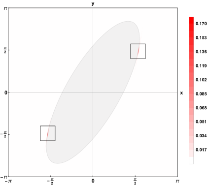
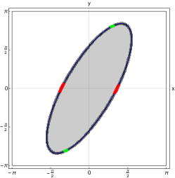
Figure 3: Left: Characteristic function D 1 , 3 , π 6 2 π superscript subscript 𝐷 1 3 𝜋 6
2 𝜋 D_{1,3,\frac{\pi}{6}}^{2\pi} | ⟨ D 1 , 3 , π 6 2 π , ψ 10 , − 3 , 𝐲 ( h ) ⟩ 2 | subscript superscript subscript 𝐷 1 3 𝜋 6
2 𝜋 superscript subscript 𝜓 10 3 𝐲
h
2 \left\lvert\left\langle D_{1,3,\frac{\pi}{6}}^{2\pi},\psi_{10,-3,\mathbf{y}}^{(\mathrm{h})}\right\rangle_{2}\right\rvert 𝐲 ∈ 𝒫 ( 𝐌 10 ) 𝐲 𝒫 subscript 𝐌 10 \mathbf{y}\in\mathcal{P}(\mathbf{M}_{10}) ∑ ℓ = − 2 j / 2 + 1 2 j / 2 − 1 | ⟨ D 1 , 3 , π 6 2 π , ψ 10 , ℓ , 𝐲 ( i ) ⟩ 2 | superscript subscript ℓ superscript 2 𝑗 2 1 superscript 2 𝑗 2 1 subscript superscript subscript 𝐷 1 3 𝜋 6
2 𝜋 superscript subscript 𝜓 10 ℓ 𝐲
𝑖
2 \sum\limits_{\ell=-2^{j/2}+1}^{2^{j/2}-1}\left\lvert\left\langle D_{1,3,\frac{\pi}{6}}^{2\pi},\psi_{10,\ell,\mathbf{y}}^{(i)}\right\rangle_{2}\right\rvert 𝐲 ∈ 𝒫 ( 𝐌 10 ) 𝐲 𝒫 subscript 𝐌 10 \mathbf{y}\in\mathcal{P}(\mathbf{M}_{10}) i ∈ { h , v } 𝑖 h v i\in\left\{\mathrm{h},\mathrm{v}\right\}
For a , b > 0 𝑎 𝑏
0 a,b>0 D a , b ( 𝐱 ) : = D ( a − 1 x 1 , b − 1 x 2 ) D_{a,b}(\mathbf{x})\mathrel{\mathop{:}}=D(a^{-1}x_{1},b^{-1}x_{2}) a 𝑎 a b 𝑏 b
ℱ [ D a , b ] ( 𝝃 ) = a b J 1 ( | ( a ξ 1 , b ξ 2 ) | 2 ) 2 π | ( a ξ 1 , b ξ 2 ) | 2 . ℱ delimited-[] subscript 𝐷 𝑎 𝑏
𝝃 𝑎 𝑏 subscript 𝐽 1 subscript 𝑎 subscript 𝜉 1 𝑏 subscript 𝜉 2 2 2 𝜋 subscript 𝑎 subscript 𝜉 1 𝑏 subscript 𝜉 2 2 \mathcal{F}\left[D_{a,b}\right](\boldsymbol{\xi})=\frac{ab\,J_{1}\bigl{(}\left\lvert(a\xi_{1},b\xi_{2})\right\rvert_{2}\bigr{)}}{2\pi\left\lvert(a\xi_{1},b\xi_{2})\right\rvert_{2}}.
If we further rotate the function D a , b subscript 𝐷 𝑎 𝑏
D_{a,b} γ ∈ [ 0 , 2 π ) 𝛾 0 2 𝜋 \gamma\in[0,2\pi) D a , b , γ ( 𝐱 ) : = D a , b ( 𝐑 γ 𝐱 ) D_{a,b,\gamma}(\mathbf{x})\mathrel{\mathop{:}}=D_{a,b}\left(\mathbf{R}_{\gamma}\,\mathbf{x}\right) ℱ [ D a , b , γ ] ( 𝝃 ) = ℱ [ D a , b ] ( 𝐑 T 𝝃 ) ℱ delimited-[] subscript 𝐷 𝑎 𝑏 𝛾
𝝃 ℱ delimited-[] subscript 𝐷 𝑎 𝑏
superscript 𝐑 T 𝝃 \mathcal{F}\left[D_{a,b,\gamma}\right](\boldsymbol{\xi})=\mathcal{F}\left[D_{a,b}\right](\mathbf{R}^{\mathrm{T}}\boldsymbol{\xi})
In order to calculate the shearlet coefficients of a rotated ellipse we consider the 2 π 2 𝜋 2\pi D a , b , γ 2 π ( 𝐱 ) superscript subscript 𝐷 𝑎 𝑏 𝛾
2 𝜋 𝐱 D_{a,b,\gamma}^{2\pi}(\mathbf{x}) Eq. 15
c 𝐤 ( D a , b , γ 2 π ) = ℱ [ D a , b , γ ] ( 𝐤 ) , 𝐤 ∈ ℤ 2 , formulae-sequence subscript 𝑐 𝐤 superscript subscript 𝐷 𝑎 𝑏 𝛾
2 𝜋 ℱ delimited-[] subscript 𝐷 𝑎 𝑏 𝛾
𝐤 𝐤 superscript ℤ 2 c_{\mathbf{k}}(D_{a,b,\gamma}^{2\pi})=\mathcal{F}\left[D_{a,b,\gamma}\right](\mathbf{k}),\;\mathbf{k}\in\mathbb{Z}^{2},
and Parseval’s identity finally gives
⟨ D a , b , γ 2 π , ψ j , ℓ , 𝐲 ( i ) ⟩ 2 = ∑ 𝐤 ∈ ℤ 2 ℱ [ D a , b , γ ] ( 𝐤 ) Ψ j , ℓ ( i ) ( 𝐤 ) e 2 π i 𝐤 T 𝐲 ~ . subscript superscript subscript 𝐷 𝑎 𝑏 𝛾
2 𝜋 subscript superscript 𝜓 𝑖 𝑗 ℓ 𝐲
2 subscript 𝐤 superscript ℤ 2 ℱ delimited-[] subscript 𝐷 𝑎 𝑏 𝛾
𝐤 subscript superscript Ψ 𝑖 𝑗 ℓ
𝐤 superscript e 2 𝜋 i superscript 𝐤 T ~ 𝐲 \left\langle D_{a,b,\gamma}^{2\pi},\psi^{(i)}_{j,\ell,\mathbf{y}}\right\rangle_{2}=\sum_{\mathbf{k}\in\mathbb{Z}^{2}}\mathcal{F}\left[D_{a,b,\gamma}\right](\mathbf{k})\,\Psi^{(i)}_{j,\ell}(\mathbf{k})\,\mathrm{e}^{2\pi\mathrm{i}\mathbf{k}^{\mathrm{T}}\widetilde{\mathbf{y}}}. (11)
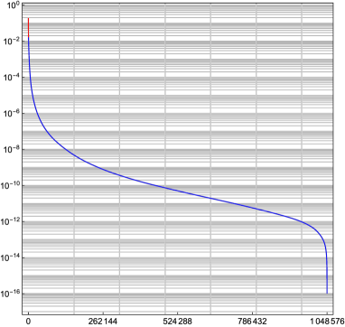
In our numerical example we calculate the inner product Eq. 11 Mathematica 12 . We fix the characteristic function of the rotated ellipse D 1 , 3 , π 6 2 π superscript subscript 𝐷 1 3 𝜋 6
2 𝜋 D_{1,3,\frac{\pi}{6}}^{2\pi} Figure 3 g 0.025 ∈ 𝒲 ∞ subscript 𝑔 0.025 superscript 𝒲 g_{0.025}\in\mathcal{W}^{\infty} Eq. 4 j = 10 𝑗 10 j=10 𝐌 10 = 2 10 𝐈 2 subscript 𝐌 10 superscript 2 10 subscript 𝐈 2 \mathbf{M}_{10}=2^{10}\,\mathbf{I}_{2} 𝐈 2 subscript 𝐈 2 \mathbf{I}_{2} Eq. 11 𝒫 ( 𝐌 10 ) 𝒫 subscript 𝐌 10 \mathcal{P}(\mathbf{M}_{10}) 1024 × 1024 1024 1024 1024\times 1024 1024 × 1024 1024 1024 1024\times 1024 ψ j , ℓ , 𝐲 ( i ) , 𝐲 ∈ 𝒫 ( 𝐌 10 ) superscript subscript 𝜓 𝑗 ℓ 𝐲
𝑖 𝐲
𝒫 subscript 𝐌 10 \psi_{j,\ell,\mathbf{y}}^{(i)},\;\mathbf{y}\in\mathcal{P}(\mathbf{M}_{10})
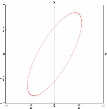
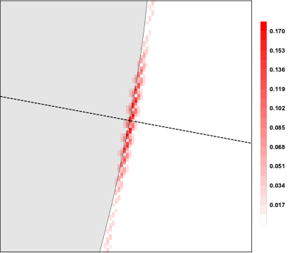
Figure 4: Left: Zoom into the upper right window from the left image of Figure 3 | ⟨ D 1 , 3 , π 6 2 π , ψ 10 , − 3 , 𝐲 ( h ) ⟩ 2 | subscript superscript subscript 𝐷 1 3 𝜋 6
2 𝜋 superscript subscript 𝜓 10 3 𝐲
h
2 \left\lvert\left\langle D_{1,3,\frac{\pi}{6}}^{2\pi},\psi_{10,-3,\mathbf{y}}^{(\mathrm{h})}\right\rangle_{2}\right\rvert 𝐲 ∈ 𝒫 ( 𝐌 10 ) 𝐲 𝒫 subscript 𝐌 10 \mathbf{y}\in\mathcal{P}(\mathbf{M}_{10})
On the left side of Figure 3 ℓ = − 3 ℓ 3 \ell=-3
| ⟨ D 1 , 3 , π 6 2 π , ψ 10 , − 3 , 𝐲 ( h ) ⟩ 2 | subscript superscript subscript 𝐷 1 3 𝜋 6
2 𝜋 superscript subscript 𝜓 10 3 𝐲
h
2 \left\lvert\left\langle D_{1,3,\frac{\pi}{6}}^{2\pi},\psi_{10,-3,\mathbf{y}}^{(\mathrm{h})}\right\rangle_{2}\right\rvert
are very close to zero except for the pattern points 𝐲 ∈ 𝒫 ( 𝐌 10 ) 𝐲 𝒫 subscript 𝐌 10 \mathbf{y}\in\mathcal{P}(\mathbf{M}_{10}) ψ 10 , − 3 , 𝐲 ( h ) superscript subscript 𝜓 10 3 𝐲
h \psi_{10,-3,\mathbf{y}}^{(\mathrm{h})} 𝐱 ∈ ∂ D 1 , 3 , π 6 2 π 𝐱 superscript subscript 𝐷 1 3 𝜋 6
2 𝜋 \mathbf{x}\in\partial D_{1,3,\frac{\pi}{6}}^{2\pi} θ 10 , − 3 ( h ) superscript subscript 𝜃 10 3
h \theta_{10,-3}^{(\mathrm{h})}
To make this more clear, the left image of Figure 4 θ 10 , − 3 ( h ) superscript subscript 𝜃 10 3
h \theta_{10,-3}^{(\mathrm{h})} ψ 10 , − 3 , 𝐲 ( h ) superscript subscript 𝜓 10 3 𝐲
h \psi_{10,-3,\mathbf{y}}^{(\mathrm{h})} ∂ D 1 , 3 , π 6 2 π superscript subscript 𝐷 1 3 𝜋 6
2 𝜋 \partial D_{1,3,\frac{\pi}{6}}^{2\pi} Eq. 11 Figure 4 | ⟨ D 1 , 3 , π 6 2 π , ψ 10 , − 3 , 𝐲 ( h ) ⟩ 2 | subscript superscript subscript 𝐷 1 3 𝜋 6
2 𝜋 superscript subscript 𝜓 10 3 𝐲
h
2 \left\lvert\left\langle D_{1,3,\frac{\pi}{6}}^{2\pi},\psi_{10,-3,\mathbf{y}}^{(\mathrm{h})}\right\rangle_{2}\right\rvert 𝐲 ∈ 𝒫 ( 𝐌 10 ) 𝐲 𝒫 subscript 𝐌 10 \mathbf{y}\in\mathcal{P}(\mathbf{M}_{10}) Figure 3 i ∈ { h , v } 𝑖 h v i\in\left\{\mathrm{h},\mathrm{v}\right\} ℓ = − 2 j / 2 + 1 , … , 2 j / 2 − 1 ℓ superscript 2 𝑗 2 1 … superscript 2 𝑗 2 1
\ell=-2^{j/2}+1,\ldots,2^{j/2}-1 Figure 3
∑ ℓ = − 2 j / 2 + 1 2 j / 2 − 1 | ⟨ D 1 , 3 , π 6 2 π , ψ 10 , ℓ , 𝐲 ( i ) ⟩ 2 | , i ∈ { h , v } , 𝐲 ∈ 𝒫 ( 𝐌 10 ) , formulae-sequence superscript subscript ℓ superscript 2 𝑗 2 1 superscript 2 𝑗 2 1 subscript superscript subscript 𝐷 1 3 𝜋 6
2 𝜋 superscript subscript 𝜓 10 ℓ 𝐲
𝑖
2 𝑖
h v 𝐲 𝒫 subscript 𝐌 10 \sum\limits_{\ell=-2^{j/2}+1}^{2^{j/2}-1}\left\lvert\left\langle D_{1,3,\frac{\pi}{6}}^{2\pi},\psi_{10,\ell,\mathbf{y}}^{(i)}\right\rangle_{2}\right\rvert,\qquad i\in\left\{\mathrm{h},\mathrm{v}\right\},\,\,\mathbf{y}\in\mathcal{P}(\mathbf{M}_{10}),
and one can clearly see the only significant coefficients for all the directions are exact on the boundary of D 1 , 3 , π 6 2 π superscript subscript 𝐷 1 3 𝜋 6
2 𝜋 D_{1,3,\frac{\pi}{6}}^{2\pi}
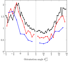
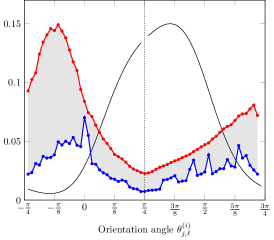
Figure 5: Left: U j , ℓ ( i ) subscript superscript 𝑈 𝑖 𝑗 ℓ
U^{(i)}_{j,\ell} j = 4 𝑗 4 j=4 j = 6 𝑗 6 j=6 j = 8 𝑗 8 j=8 L j , ℓ ( i ) subscript superscript 𝐿 𝑖 𝑗 ℓ
L^{(i)}_{j,\ell} j = 8 𝑗 8 j=8 ℓ ∈ ℤ ℓ ℤ \ell\in\mathbb{Z} | ℓ | < 2 j / 2 ℓ superscript 2 𝑗 2 \left\lvert\ell\right\rvert<2^{j/2} L 8 , − 8 ( h ) subscript superscript 𝐿 h 8 8
L^{(\mathrm{h})}_{8,-8} L 8 , − 8 ( v ) subscript superscript 𝐿 v 8 8
L^{(\mathrm{v})}_{8,-8} L j , ℓ ( i ) , max subscript superscript 𝐿 𝑖 max
𝑗 ℓ
L^{(i),\mathrm{max}}_{j,\ell} L j , ℓ ( i ) , min subscript superscript 𝐿 𝑖 min
𝑗 ℓ
L^{(i),\mathrm{min}}_{j,\ell} 1 20 κ ( x ) 1 20 𝜅 𝑥 \frac{1}{20}\kappa(x)
Besides the visual representations of the detection of step discontinuities with trigonometric polynomial shearlets, we want to illustrate the upper and lower estimates given in the two main theorems. In order to do so for the upper bound, we compute the quantity
U j , ℓ ( i ) : = max 𝐲 ∈ 𝒫 ( 𝐌 j ) | ⟨ D 1 , 3 , π 6 2 π , ψ j , ℓ , 𝐲 ( i ) ⟩ 2 | ∑ Q ∈ 𝒬 j 1 ( 1 + 2 j | 𝐱 0 − 2 π 𝐲 ~ | 2 2 ) − q ( 1 + 2 j / 2 | sin ( θ j , ℓ ( i ) − γ ) | ) − 5 / 2 . U^{(i)}_{j,\ell}\mathrel{\mathop{:}}=\max\limits_{\mathbf{y}\in\mathcal{P}(\mathbf{M}_{j})}\frac{\left\lvert\left\langle D_{1,3,\frac{\pi}{6}}^{2\pi},\psi_{j,\ell,\mathbf{y}}^{(i)}\right\rangle_{2}\right\rvert}{\sum\limits_{Q\in\mathcal{Q}_{j}^{1}}\left(1+2^{j}\left\lvert\mathbf{x}_{0}-2\pi\widetilde{\mathbf{y}}\right\rvert_{2}^{2}\right)^{-q}\left(1+2^{j/2}\left\lvert\sin(\theta_{j,\ell}^{(i)}-\gamma)\right\rvert\right)^{-5/2}}.
In the left graph of Figure 5 U j , ℓ ( i ) subscript superscript 𝑈 𝑖 𝑗 ℓ
U^{(i)}_{j,\ell} θ j , ℓ ( i ) superscript subscript 𝜃 𝑗 ℓ
𝑖 \theta_{j,\ell}^{(i)} U j , ℓ ( i ) subscript superscript 𝑈 𝑖 𝑗 ℓ
U^{(i)}_{j,\ell} j 𝑗 j ℓ ℓ \ell Theorem 3.1
For the lower bound, we collect all pattern points 𝐲 ∈ 𝒫 ( 𝐌 j ) 𝐲 𝒫 subscript 𝐌 𝑗 \mathbf{y}\in\mathcal{P}(\mathbf{M}_{j}) 𝐱 0 ∈ ∂ T subscript 𝐱 0 𝑇 \mathbf{x}_{0}\in\partial T ( cos γ , sin γ ) T superscript 𝛾 𝛾 T (\cos{\gamma},\sin{\gamma})^{\mathrm{T}} | 𝐱 0 − 2 π 𝐲 ~ | 2 ≤ C 2 − j / 2 subscript subscript 𝐱 0 2 𝜋 ~ 𝐲 2 𝐶 superscript 2 𝑗 2 \left\lvert\mathbf{x}_{0}-2\pi\widetilde{\mathbf{y}}\right\rvert_{2}\leq C\,2^{-j/2} θ j , ℓ ( i ) ≤ γ ≤ θ j , ℓ + 1 ( i ) superscript subscript 𝜃 𝑗 ℓ
𝑖 𝛾 superscript subscript 𝜃 𝑗 ℓ 1
𝑖 \theta_{j,\ell}^{(i)}\leq\gamma\leq\theta_{j,\ell+1}^{(i)} L j , ℓ ( i ) subscript superscript 𝐿 𝑖 𝑗 ℓ
L^{(i)}_{j,\ell} L j , ℓ ( i ) subscript superscript 𝐿 𝑖 𝑗 ℓ
L^{(i)}_{j,\ell} Figure 5 j = 8 𝑗 8 j=8 ℓ ∈ ℤ ℓ ℤ \ell\in\mathbb{Z} | ℓ | < 2 j / 2 ℓ superscript 2 𝑗 2 \left\lvert\ell\right\rvert<2^{j/2} L 8 , − 8 ( h ) subscript superscript 𝐿 h 8 8
L^{(\mathrm{h})}_{8,-8} L 8 , − 8 ( v ) subscript superscript 𝐿 v 8 8
L^{(\mathrm{v})}_{8,-8} 𝐱 0 ∈ ∂ T subscript 𝐱 0 𝑇 \mathbf{x}_{0}\in\partial T ( cos γ , sin γ ) T superscript 𝛾 𝛾 T (\cos{\gamma},\sin{\gamma})^{\mathrm{T}} θ 8 , − 8 ( i ) ≤ γ ≤ θ 8 , − 7 ( i ) superscript subscript 𝜃 8 8
𝑖 𝛾 superscript subscript 𝜃 8 7
𝑖 \theta_{8,-8}^{(i)}\leq\gamma\leq\theta_{8,-7}^{(i)} i ∈ { h , v } 𝑖 h v i\in\left\{\mathrm{h},\mathrm{v}\right\} Theorem 3.2 ψ 8 , − 8 , 𝐲 ( i ) subscript superscript 𝜓 𝑖 8 8 𝐲
\psi^{(i)}_{8,-8,\mathbf{y}} 𝐲 ∈ L 8 , − 8 ( i ) 𝐲 subscript superscript 𝐿 𝑖 8 8
\mathbf{y}\in L^{(i)}_{8,-8}
L j , ℓ ( i ) , max : = max 𝐲 ∈ L j , ℓ ( i ) | ⟨ D 1 , 3 , π 6 2 π , ψ j , ℓ , 𝐲 ( i ) ⟩ 2 | , L j , ℓ ( i ) , min : = min 𝐲 ∈ L j , ℓ ( i ) | ⟨ D 1 , 3 , π 6 2 π , ψ j , ℓ , 𝐲 ( i ) ⟩ 2 | L^{(i),\mathrm{max}}_{j,\ell}\mathrel{\mathop{:}}=\max\limits_{\mathbf{y}\in L^{(i)}_{j,\ell}}\left\lvert\left\langle D_{1,3,\frac{\pi}{6}}^{2\pi},\psi_{j,\ell,\mathbf{y}}^{(i)}\right\rangle_{2}\right\rvert,\quad L^{(i),\mathrm{min}}_{j,\ell}\mathrel{\mathop{:}}=\min\limits_{\mathbf{y}\in L^{(i)}_{j,\ell}}\left\lvert\left\langle D_{1,3,\frac{\pi}{6}}^{2\pi},\psi_{j,\ell,\mathbf{y}}^{(i)}\right\rangle_{2}\right\rvert
and show them in the right graph of Figure 5 θ j , ℓ ( i ) superscript subscript 𝜃 𝑗 ℓ
𝑖 \theta_{j,\ell}^{(i)} L j , ℓ ( i ) , min subscript superscript 𝐿 𝑖 min
𝑗 ℓ
L^{(i),\mathrm{min}}_{j,\ell} Theorem 3.2 ∂ D 1 , 3 , π 6 subscript 𝐷 1 3 𝜋 6
\partial D_{1,3,\frac{\pi}{6}} 𝜸 ( x ) = 1 2 ( 3 cos x + 3 sin x , 3 3 sin x − cos x ) T 𝜸 𝑥 1 2 superscript 3 𝑥 3 𝑥 3 3 𝑥 𝑥 T \boldsymbol{\gamma}(x)=\frac{1}{2}\bigl{(}\sqrt{3}\cos x+3\sin x,3\sqrt{3}\sin x-\cos x\bigr{)}^{\mathrm{T}} κ ( x ) = 3 ( 5 + 4 cos ( 2 x ) ) − 3 / 2 𝜅 𝑥 3 superscript 5 4 2 𝑥 3 2 \kappa(x)=3\left(5+4\cos(2x)\right)^{-3/2} Figure 5 κ ( x ) 𝜅 𝑥 \kappa(x) 𝐱 0 ∈ ∂ T subscript 𝐱 0 𝑇 \mathbf{x}_{0}\in\partial T 𝐱 0 subscript 𝐱 0 \mathbf{x}_{0} θ j , ℓ ( i ) subscript superscript 𝜃 𝑖 𝑗 ℓ
\theta^{(i)}_{j,\ell} | ℓ | < 2 j / 2 ℓ superscript 2 𝑗 2 \left\lvert\ell\right\rvert<2^{j/2} Theorem 3.2 L j , ℓ ( i ) , max , L j , ℓ ( i ) , min subscript superscript 𝐿 𝑖 max
𝑗 ℓ
subscript superscript 𝐿 𝑖 min
𝑗 ℓ
L^{(i),\mathrm{max}}_{j,\ell},L^{(i),\mathrm{min}}_{j,\ell}
5 Auxiliary results
For two-dimensional vector norms we use the notation
| 𝐱 | p : = { ( | x 1 | p + | x 2 | p ) 1 / p , if 1 ≤ p < ∞ , max { | x 1 | , | x 2 | } , if p = ∞ \left\lvert\mathbf{x}\right\rvert_{p}\mathrel{\mathop{:}}=\begin{cases}\left(\left\lvert x_{1}\right\rvert^{p}+\left\lvert x_{2}\right\rvert^{p}\right)^{1/p},&\text{if }1\leq p<\infty,\\
\max\left\{\left\lvert x_{1}\right\rvert,\left\lvert x_{2}\right\rvert\right\},&\text{if }p=\infty\end{cases}
and for binary relations and exponentials of vectors we write 𝐱 ≤ 𝐲 𝐱 𝐲 \mathbf{x}\leq\mathbf{y} x 1 ≤ y 1 subscript 𝑥 1 subscript 𝑦 1 x_{1}\leq y_{1} x 2 ≤ y 2 subscript 𝑥 2 subscript 𝑦 2 x_{2}\leq y_{2} 𝐱 𝐲 : = x 1 y 1 x 2 y 2 \mathbf{x}^{\mathbf{y}}\mathrel{\mathop{:}}=x_{1}^{y_{1}}\,x_{2}^{y_{2}} 𝐱 β : = 𝐱 β 𝟏 = x 1 β x 2 β \mathbf{x}^{\beta}\mathrel{\mathop{:}}=\mathbf{x}^{\beta\mathbf{1}}=x_{1}^{\beta}\,x_{2}^{\beta} β ∈ ℝ 𝛽 ℝ \beta\in\mathbb{R} 𝐤 , 𝐧 ∈ ℕ 0 2 𝐤 𝐧
superscript subscript ℕ 0 2 \mathbf{k},\mathbf{n}\in\mathbb{N}_{0}^{2} 𝐤 ≤ 𝐧 𝐤 𝐧 \mathbf{k}\leq\mathbf{n} n ∈ ℕ 0 𝑛 subscript ℕ 0 n\in\mathbb{N}_{0} 𝐤 ≤ n 𝟏 𝐤 𝑛 1 \mathbf{k}\leq n\mathbf{1} 𝐤 ! : = k 1 ! k 2 ! \mathbf{k}!\mathrel{\mathop{:}}=k_{1}!\,k_{2}!
( 𝐧 𝐤 ) : = 𝐧 ! 𝐤 ! ( 𝐧 − 𝐤 ) ! = ( n 1 k 1 ) ( n 2 k 2 ) , ( n 𝐤 ) : = n ! 𝐤 ! ( n − | 𝐤 | 1 ) ! . \binom{\mathbf{n}}{\mathbf{k}}\mathrel{\mathop{:}}=\frac{\mathbf{n}!}{\mathbf{k}!(\mathbf{n}-\mathbf{k})!}=\binom{n_{1}}{k_{1}}\,\binom{n_{2}}{k_{2}},\quad\binom{n}{\mathbf{k}}\mathrel{\mathop{:}}=\frac{n!}{\mathbf{k}!(n-\left\lvert\mathbf{k}\right\rvert_{1})!}.
The Fourier coefficients of a function f ∈ L 1 ( 𝕋 2 ) 𝑓 subscript 𝐿 1 superscript 𝕋 2 f\in L_{1}(\mathbb{T}^{2})
c 𝐤 ( f ) : = ( 2 π ) − 2 ∫ 𝕋 2 f ( 𝐱 ) e − i 𝐤 T 𝐱 d 𝐱 , 𝐤 ∈ ℤ 2 . c_{\mathbf{k}}(f)\mathrel{\mathop{:}}=(2\pi)^{-2}\int_{\mathbb{T}^{2}}f(\mathbf{x})\,\mathrm{e}^{-\mathrm{i}\mathbf{k}^{\mathrm{T}}\mathbf{x}}\,\mathrm{d}\mathbf{x},\qquad\mathbf{k}\in\mathbb{Z}^{2}.
The Fourier transform of f ∈ L 1 ( ℝ 2 ) 𝑓 subscript 𝐿 1 superscript ℝ 2 f\in L_{1}(\mathbb{R}^{2})
ℱ [ f ] ( 𝐱 ) : = ℱ f ( 𝐱 ) : = ( 2 π ) − 2 ∫ ℝ 2 f ( 𝝃 ) e − i 𝝃 T 𝐱 d 𝝃 , 𝐱 ∈ ℝ 2 , \mathcal{F}[f](\mathbf{x})\mathrel{\mathop{:}}=\mathcal{F}f(\mathbf{x})\mathrel{\mathop{:}}=(2\pi)^{-2}\int_{\mathbb{R}^{2}}f(\boldsymbol{\xi})\,\mathrm{e}^{-\mathrm{i}\boldsymbol{\xi}^{\mathrm{T}}\mathbf{x}}\,\mathrm{d}\boldsymbol{\xi},\qquad\mathbf{x}\in\mathbb{R}^{2},
and we have the operator
ℱ − 1 [ f ] ( 𝐱 ) : = ℱ − 1 f ( 𝐱 ) : = ∫ ℝ 2 f ( 𝝃 ) e i 𝝃 T 𝐱 d 𝝃 , 𝐱 ∈ ℝ 2 . \mathcal{F}^{-1}[f](\mathbf{x})\mathrel{\mathop{:}}=\mathcal{F}^{-1}f(\mathbf{x})\mathrel{\mathop{:}}=\int_{\mathbb{R}^{2}}f(\boldsymbol{\xi})\,\mathrm{e}^{\mathrm{i}\boldsymbol{\xi}^{\mathrm{T}}\mathbf{x}}\,\mathrm{d}\boldsymbol{\xi},\qquad\mathbf{x}\in\mathbb{R}^{2}.
For f ∈ L 1 ( ℝ 2 ) 𝑓 subscript 𝐿 1 superscript ℝ 2 f\in L_{1}(\mathbb{R}^{2}) ℱ f ∈ L 1 ( ℝ 2 ) ℱ 𝑓 subscript 𝐿 1 superscript ℝ 2 \mathcal{F}f\in L_{1}(\mathbb{R}^{2}) f ( 𝐱 ) = ℱ ℱ − 1 f ( 𝐱 ) = ℱ − 1 ℱ f ( 𝐱 ) 𝑓 𝐱 ℱ superscript ℱ 1 𝑓 𝐱 superscript ℱ 1 ℱ 𝑓 𝐱 f(\mathbf{x})=\mathcal{F}\mathcal{F}^{-1}f(\mathbf{x})=\mathcal{F}^{-1}\mathcal{F}f(\mathbf{x}) 𝐱 ∈ ℝ 2 𝐱 superscript ℝ 2 \mathbf{x}\in\mathbb{R}^{2} q ∈ ℕ 0 𝑞 subscript ℕ 0 q\in\mathbb{N}_{0} 𝐫 ∈ ℕ 0 2 𝐫 superscript subscript ℕ 0 2 \mathbf{r}\in\mathbb{N}_{0}^{2} | 𝐫 | 1 ≤ q subscript 𝐫 1 𝑞 \left\lvert\mathbf{r}\right\rvert_{1}\leq q f ∈ L 1 ( ℝ 2 ) 𝑓 subscript 𝐿 1 superscript ℝ 2 f\in L_{1}(\mathbb{R}^{2}) ( i 𝐱 ) q f ∈ L 1 ( ℝ 2 ) superscript i 𝐱 𝑞 𝑓 subscript 𝐿 1 superscript ℝ 2 (\mathrm{i}\,\mathbf{x})^{q}\,f\in L_{1}(\mathbb{R}^{2}) ℱ f ∈ C q ( ℝ 2 ) ℱ 𝑓 superscript 𝐶 𝑞 superscript ℝ 2 \mathcal{F}f\in C^{q}(\mathbb{R}^{2})
∂ 𝐫 ℱ f ( 𝝃 ) = ℱ [ ( i 𝐱 ) 𝐫 f ( 𝐱 ) ] ( 𝝃 ) . superscript 𝐫 ℱ 𝑓 𝝃 ℱ delimited-[] superscript i 𝐱 𝐫 𝑓 𝐱 𝝃 \partial^{\mathbf{r}}\mathcal{F}f(\boldsymbol{\xi})=\mathcal{F}\left[(\mathrm{i}\,\mathbf{x})^{\mathbf{r}}\,f(\mathbf{x})\right](\boldsymbol{\xi}). (12)
Moreover for f ∈ C q ( ℝ 2 ) 𝑓 superscript 𝐶 𝑞 superscript ℝ 2 f\in C^{q}(\mathbb{R}^{2}) ∂ 𝐫 f ∈ L 1 ( ℝ 2 ) superscript 𝐫 𝑓 subscript 𝐿 1 superscript ℝ 2 \partial^{\mathbf{r}}f\in L_{1}(\mathbb{R}^{2})
ℱ [ ∂ 𝐫 f ] ( 𝝃 ) = ( i 𝝃 ) 𝐫 ℱ f ( 𝝃 ) . ℱ delimited-[] superscript 𝐫 𝑓 𝝃 superscript i 𝝃 𝐫 ℱ 𝑓 𝝃 \mathcal{F}\left[\partial^{\mathbf{r}}f\right](\boldsymbol{\xi})=(\mathrm{i}\,\boldsymbol{\xi})^{\mathbf{r}}\,\mathcal{F}f(\boldsymbol{\xi}). (13)
It is well known that there are constants C 1 ( q , f ) , C 2 ( q , f ) > 0 subscript 𝐶 1 𝑞 𝑓 subscript 𝐶 2 𝑞 𝑓
0 C_{1}(q,f),C_{2}(q,f)>0 f ∈ C 0 q ( ℝ 2 ) 𝑓 superscript subscript 𝐶 0 𝑞 superscript ℝ 2 f\in C_{0}^{q}(\mathbb{R}^{2}) q ∈ ℕ 0 𝑞 subscript ℕ 0 q\in\mathbb{N}_{0} 𝐱 ∈ ℝ 2 𝐱 superscript ℝ 2 \mathbf{x}\in\mathbb{R}^{2}
| ℱ f ( 𝐱 ) | ≤ C 1 ( q , f ) ( 1 + | 𝐱 | 2 ) q , | ℱ − 1 f ( 𝐱 ) | ≤ C 2 ( q , f ) ( 1 + | 𝐱 | 2 ) q . formulae-sequence ℱ 𝑓 𝐱 subscript 𝐶 1 𝑞 𝑓 superscript 1 subscript 𝐱 2 𝑞 superscript ℱ 1 𝑓 𝐱 subscript 𝐶 2 𝑞 𝑓 superscript 1 subscript 𝐱 2 𝑞 \lvert\mathcal{F}f(\mathbf{x})\rvert\leq\frac{C_{1}(q,f)}{\left(1+\lvert\mathbf{x}\rvert_{2}\right)^{q}},\qquad\qquad\lvert\mathcal{F}^{-1}f(\mathbf{x})\rvert\leq\frac{C_{2}(q,f)}{\left(1+\lvert\mathbf{x}\rvert_{2}\right)^{q}}. (14)
The sum in Eq. 10 𝐱 ∈ 𝕋 2 𝐱 superscript 𝕋 2 \mathbf{x}\in\mathbb{T}^{2} f 2 π ∈ L 1 ( 𝕋 2 ) superscript 𝑓 2 𝜋 subscript 𝐿 1 superscript 𝕋 2 f^{2\pi}\in L_{1}(\mathbb{T}^{2})
c 𝐤 ( f 2 π ) = ℱ f ( 𝐤 ) , 𝐤 ∈ ℤ 2 . formulae-sequence subscript 𝑐 𝐤 superscript 𝑓 2 𝜋 ℱ 𝑓 𝐤 𝐤 superscript ℤ 2 c_{\mathbf{k}}(f^{2\pi})=\mathcal{F}f(\mathbf{k}),\qquad\mathbf{k}\in\mathbb{Z}^{2}. (15)
It is a consequence of Eq. 14 [33 , Corollary VII.2.6] that for a function f ∈ C 0 q ( ℝ 2 ) 𝑓 superscript subscript 𝐶 0 𝑞 superscript ℝ 2 f\in C_{0}^{q}(\mathbb{R}^{2}) q > 2 𝑞 2 q>2
∑ 𝐤 ∈ ℤ 2 ℱ f ( 𝐤 ) e i 𝐤 T 𝐱 = ∑ 𝐧 ∈ ℤ 2 f ( 𝐱 + 2 π 𝐧 ) = f 2 π ( 𝐱 ) subscript 𝐤 superscript ℤ 2 ℱ 𝑓 𝐤 superscript e i superscript 𝐤 T 𝐱 subscript 𝐧 superscript ℤ 2 𝑓 𝐱 2 𝜋 𝐧 superscript 𝑓 2 𝜋 𝐱 \sum_{\mathbf{k}\in\mathbb{Z}^{2}}\mathcal{F}f(\mathbf{k})\,\mathrm{e}^{\mathrm{i}\mathbf{k}^{\mathrm{T}}\mathbf{x}}=\sum_{\mathbf{n}\in\mathbb{Z}^{2}}f(\mathbf{x}+2\pi\mathbf{n})=f^{2\pi}(\mathbf{x}) (16)
holds true for all 𝐱 ∈ ℝ 2 𝐱 superscript ℝ 2 \mathbf{x}\in\mathbb{R}^{2}
In the following we prepare the proof of Theorem 3.1 i = h 𝑖 h i=\mathrm{h}
Lemma 5.1 .
For i ∈ { h , v } 𝑖 h v i\in\{\mathrm{h},\mathrm{v}\} q ∈ ℕ 0 𝑞 subscript ℕ 0 q\in\mathbb{N}_{0} Ψ ( i ) ∈ 𝒲 2 q superscript Ψ 𝑖 subscript superscript 𝒲 𝑞 2 \Psi^{(i)}\in\mathcal{W}^{q}_{2} 𝐫 ∈ ℕ 0 2 𝐫 superscript subscript ℕ 0 2 \mathbf{r}\in\mathbb{N}_{0}^{2} | 𝐫 | 1 ≤ q subscript 𝐫 1 𝑞 \left\lvert\mathbf{r}\right\rvert_{1}\leq q 𝐑 γ subscript 𝐑 𝛾 \mathbf{R}_{\gamma} γ ∈ [ 0 , 2 π ) 𝛾 0 2 𝜋 \gamma\in[0,2\pi)
| ∂ 𝐫 Ψ j , ℓ ( i ) ( 𝐑 γ 𝝃 ) | ≤ C ( q ) 2 − j | 𝐫 | 1 ( 1 + 2 ( j + 1 ) / 2 | sin ( θ j , ℓ ( i ) − γ ) | ) r 1 ( 1 + 2 ( j + 1 ) / 2 | cos ( θ j , ℓ ( i ) − γ ) | ) r 2 . superscript 𝐫 superscript subscript Ψ 𝑗 ℓ
𝑖 subscript 𝐑 𝛾 𝝃 𝐶 𝑞 superscript 2 𝑗 subscript 𝐫 1 superscript 1 superscript 2 𝑗 1 2 superscript subscript 𝜃 𝑗 ℓ
𝑖 𝛾 subscript 𝑟 1 superscript 1 superscript 2 𝑗 1 2 superscript subscript 𝜃 𝑗 ℓ
𝑖 𝛾 subscript 𝑟 2 \left\lvert\partial^{\mathbf{r}}\Psi_{j,\ell}^{(i)}(\mathbf{R}_{\gamma}\,\boldsymbol{\xi})\right\rvert\leq C(q)\,2^{-j\,\left\lvert\mathbf{r}\right\rvert_{1}}\left(1+2^{(j+1)/2}\left\lvert\sin\left(\theta_{j,\ell}^{(i)}-\gamma\right)\right\rvert\right)^{r_{1}}\left(1+2^{(j+1)/2}\left\lvert\cos\left(\theta_{j,\ell}^{(i)}-\gamma\right)\right\rvert\right)^{r_{2}}.
Proof.
We have 𝐑 γ = ( cos γ − sin γ sin γ cos γ ) subscript 𝐑 𝛾 matrix 𝛾 𝛾 𝛾 𝛾 \mathbf{R}_{\gamma}=\begin{pmatrix}\cos\gamma&-\sin\gamma\\
\sin\gamma&\cos\gamma\end{pmatrix} Eq. 6
Ψ j , ℓ ( h ) ( 𝐑 γ 𝝃 ) = g ( 2 − j / 2 ( ξ 1 sin γ + ξ 2 cos γ ) − ℓ 2 − j ( ξ 1 cos γ − ξ 2 sin γ ) ) g ~ ( 2 − j ( ξ 1 cos γ − ξ 2 sin γ ) ) . superscript subscript Ψ 𝑗 ℓ
h subscript 𝐑 𝛾 𝝃 𝑔 superscript 2 𝑗 2 subscript 𝜉 1 𝛾 subscript 𝜉 2 𝛾 ℓ superscript 2 𝑗 subscript 𝜉 1 𝛾 subscript 𝜉 2 𝛾 ~ 𝑔 superscript 2 𝑗 subscript 𝜉 1 𝛾 subscript 𝜉 2 𝛾 \Psi_{j,\ell}^{(\mathrm{h})}(\mathbf{R}_{\gamma}\,\boldsymbol{\xi})=g\left(2^{-j/2}(\xi_{1}\sin{\gamma}+\xi_{2}\cos{\gamma})-\ell\,2^{-j}(\xi_{1}\cos{\gamma}-\xi_{2}\sin{\gamma})\right)\widetilde{g}\Bigl{(}2^{-j}(\xi_{1}\cos{\gamma-}\xi_{2}\sin{\gamma})\Bigr{)}.
In this proof we will omit the long arguments of the function of the last line and simply write g 𝑔 g g ~ ~ 𝑔 \widetilde{g} 𝐦 = ( m 1 , m 2 ) T 𝐦 superscript subscript 𝑚 1 subscript 𝑚 2 T \mathbf{m}=(m_{1},m_{2})^{\mathrm{T}} | 𝐦 | 1 ≤ q subscript 𝐦 1 𝑞 \left\lvert\mathbf{m}\right\rvert_{1}\leq q
| ∂ 𝐦 g ~ | = ∥ g ~ ∥ C q 2 − j | 𝐦 | 1 | cos γ | m 1 | sin γ | m 2 ≤ C ( q ) 2 − j | 𝐦 | 1 superscript 𝐦 ~ 𝑔 subscript delimited-∥∥ ~ 𝑔 superscript 𝐶 𝑞 superscript 2 𝑗 subscript 𝐦 1 superscript 𝛾 subscript 𝑚 1 superscript 𝛾 subscript 𝑚 2 𝐶 𝑞 superscript 2 𝑗 subscript 𝐦 1 \left\lvert\partial^{\mathbf{m}}\widetilde{g}\right\rvert=\left\lVert\widetilde{g}\right\rVert_{C^{q}}\,2^{-j\left\lvert\mathbf{m}\right\rvert_{1}}\left\lvert\cos{\gamma}\right\rvert^{m_{1}}\left\lvert\sin{\gamma}\right\rvert^{m_{2}}\leq C(q)\,2^{-j\left\lvert\mathbf{m}\right\rvert_{1}}
and, since ℓ = 2 j / 2 tan ( θ j , ℓ ( h ) ) ℓ superscript 2 𝑗 2 superscript subscript 𝜃 𝑗 ℓ
h \ell=2^{j/2}\tan\left(\theta_{j,\ell}^{(\mathrm{h})}\right)
| ∂ 𝐦 g | superscript 𝐦 𝑔 \displaystyle\left\lvert\partial^{\mathbf{m}}g\right\rvert = ∥ g ∥ C q | 2 − j / 2 sin γ − ℓ 2 − j cos γ | m 1 | 2 − j / 2 cos γ + ℓ 2 − j sin γ | m 2 absent subscript delimited-∥∥ 𝑔 superscript 𝐶 𝑞 superscript superscript 2 𝑗 2 𝛾 ℓ superscript 2 𝑗 𝛾 subscript 𝑚 1 superscript superscript 2 𝑗 2 𝛾 ℓ superscript 2 𝑗 𝛾 subscript 𝑚 2 \displaystyle=\left\lVert g\right\rVert_{C^{q}}\left\lvert 2^{-j/2}\sin{\gamma}-\ell\,2^{-j}\cos\gamma\right\rvert^{m_{1}}\left\lvert 2^{-j/2}\cos{\gamma}+\ell\,2^{-j}\sin{\gamma}\right\rvert^{m_{2}}
= C 2 ( q ) 2 − j | 𝐦 | 1 ( 2 j / 2 | sin ( θ j , ℓ ( h ) − γ ) | | cos ( θ j , ℓ ( h ) ) | ) m 1 ( 2 j / 2 | cos ( θ j , ℓ ( h ) − γ ) | | cos ( θ j , ℓ ( h ) ) | ) m 2 . absent subscript 𝐶 2 𝑞 superscript 2 𝑗 subscript 𝐦 1 superscript superscript 2 𝑗 2 superscript subscript 𝜃 𝑗 ℓ
h 𝛾 superscript subscript 𝜃 𝑗 ℓ
h subscript 𝑚 1 superscript superscript 2 𝑗 2 superscript subscript 𝜃 𝑗 ℓ
h 𝛾 superscript subscript 𝜃 𝑗 ℓ
h subscript 𝑚 2 \displaystyle=C_{2}(q)\,2^{-j\left\lvert\mathbf{m}\right\rvert_{1}}\,\left(2^{j/2}\frac{\left\lvert\sin\left(\theta_{j,\ell}^{(\mathrm{h})}-\gamma\right)\right\rvert}{\left\lvert\cos\left(\theta_{j,\ell}^{(\mathrm{h})}\right)\right\rvert}\right)^{m_{1}}\left(2^{j/2}\frac{\left\lvert\cos\left(\theta_{j,\ell}^{(\mathrm{h})}-\gamma\right)\right\rvert}{\left\lvert\cos\left(\theta_{j,\ell}^{(\mathrm{h})}\right)\right\rvert}\right)^{m_{2}}.
For sufficiently smooth functions f , g : ℝ 2 → ℝ : 𝑓 𝑔
→ superscript ℝ 2 ℝ f,g:\mathbb{R}^{2}\rightarrow\mathbb{R}
∂ 𝐫 ( f g ) = ∑ 𝟎 ≤ 𝐬 ≤ 𝐫 ( 𝐫 𝐬 ) ∂ 𝐬 f ∂ 𝐫 − 𝐬 g , superscript 𝐫 𝑓 𝑔 subscript 0 𝐬 𝐫 binomial 𝐫 𝐬 superscript 𝐬 𝑓 superscript 𝐫 𝐬 𝑔 \partial^{\mathbf{r}}(fg)=\sum_{\mathbf{0}\leq\mathbf{s}\leq\mathbf{r}}\binom{\mathbf{r}}{\mathbf{s}}\partial^{\mathbf{s}}f\partial^{\mathbf{r}-\mathbf{s}}g, (17)
which together with the triangle inequality and the binomial theorem implies
| ∂ 𝐫 Ψ j , ℓ ( h ) ( 𝐑 γ 𝝃 ) | superscript 𝐫 superscript subscript Ψ 𝑗 ℓ
h subscript 𝐑 𝛾 𝝃 \displaystyle\left\lvert\partial^{\mathbf{r}}\Psi_{j,\ell}^{(\mathrm{h})}(\mathbf{R}_{\gamma}\,\boldsymbol{\xi})\right\rvert ≤ C 3 ( q ) 2 − j | 𝐫 | 1 ∑ 𝟎 ≤ 𝐬 ≤ 𝐫 ( 𝐫 𝐬 ) ( 2 j / 2 | sin ( θ j , ℓ ( h ) − γ ) | | cos ( θ j , ℓ ( h ) ) | ) s 1 ( 2 j / 2 | cos ( θ j , ℓ ( h ) − γ ) | | cos ( θ j , ℓ ( h ) ) | ) s 2 absent subscript 𝐶 3 𝑞 superscript 2 𝑗 subscript 𝐫 1 subscript 0 𝐬 𝐫 binomial 𝐫 𝐬 superscript superscript 2 𝑗 2 superscript subscript 𝜃 𝑗 ℓ
h 𝛾 superscript subscript 𝜃 𝑗 ℓ
h subscript 𝑠 1 superscript superscript 2 𝑗 2 superscript subscript 𝜃 𝑗 ℓ
h 𝛾 superscript subscript 𝜃 𝑗 ℓ
h subscript 𝑠 2 \displaystyle\leq C_{3}(q)\,2^{-j\left\lvert\mathbf{r}\right\rvert_{1}}\sum_{\mathbf{0}\leq\mathbf{s}\leq\mathbf{r}}\binom{\mathbf{r}}{\mathbf{s}}\left(2^{j/2}\frac{\left\lvert\sin\left(\theta_{j,\ell}^{(\mathrm{h})}-\gamma\right)\right\rvert}{\left\lvert\cos\left(\theta_{j,\ell}^{(\mathrm{h})}\right)\right\rvert}\right)^{s_{1}}\left(2^{j/2}\frac{\left\lvert\cos\left(\theta_{j,\ell}^{(\mathrm{h})}-\gamma\right)\right\rvert}{\left\lvert\cos\left(\theta_{j,\ell}^{(\mathrm{h})}\right)\right\rvert}\right)^{s_{2}}
≤ C 4 ( q ) 2 − j | 𝐫 | 1 ( 1 + 2 ( j + 1 ) / 2 | sin ( θ j , ℓ ( i ) − γ ) | ) r 1 ( 1 + 2 ( j + 1 ) / 2 | cos ( θ j , ℓ ( i ) − γ ) | ) r 2 , absent subscript 𝐶 4 𝑞 superscript 2 𝑗 subscript 𝐫 1 superscript 1 superscript 2 𝑗 1 2 superscript subscript 𝜃 𝑗 ℓ
𝑖 𝛾 subscript 𝑟 1 superscript 1 superscript 2 𝑗 1 2 superscript subscript 𝜃 𝑗 ℓ
𝑖 𝛾 subscript 𝑟 2 \displaystyle\leq C_{4}(q)\,2^{-j\left\lvert\mathbf{r}\right\rvert_{1}}\left(1+2^{(j+1)/2}\left\lvert\sin\left(\theta_{j,\ell}^{(i)}-\gamma\right)\right\rvert\right)^{r_{1}}\left(1+2^{(j+1)/2}\left\lvert\cos\left(\theta_{j,\ell}^{(i)}-\gamma\right)\right\rvert\right)^{r_{2}},
since 2 − 1 / 2 ≤ | cos ( θ j , ℓ ( h ) ) | ≤ 1 superscript 2 1 2 superscript subscript 𝜃 𝑗 ℓ
h 1 2^{-1/2}\leq\left\lvert\cos\left(\theta_{j,\ell}^{(\mathrm{h})}\right)\right\rvert\leq 1
In the following, we use notations and ideas from [4 , 23 ] and fix a function ϕ ∈ C 0 ∞ ( [ − π , π ] 2 ) italic-ϕ superscript subscript 𝐶 0 superscript 𝜋 𝜋 2 \phi\in C_{0}^{\infty}([-\pi,\pi]^{2}) ϕ j ( 𝐱 ) : = ϕ ( 2 j / 2 𝐱 ) \phi_{j}(\mathbf{x})\mathrel{\mathop{:}}=\phi\left(2^{j/2}\,\mathbf{x}\right) Q ∈ 𝒬 j 𝑄 subscript 𝒬 𝑗 Q\in\mathcal{Q}_{j} Eq. 9
ϕ Q ( 𝐱 ) : = ϕ ( 2 j / 2 ( x 1 + π ) − π ( 2 k 1 − 1 ) , 2 j / 2 ( x 2 + π ) − π ( 2 k 2 − 1 ) ) \phi_{Q}(\mathbf{x})\mathrel{\mathop{:}}=\phi\left(2^{j/2}(x_{1}+\pi)-\pi(2k_{1}-1),2^{j/2}(x_{2}+\pi)-\pi(2k_{2}-1)\right)
for k 1 , k 2 = 1 , … , 2 j / 2 formulae-sequence subscript 𝑘 1 subscript 𝑘 2
1 … superscript 2 𝑗 2
k_{1},k_{2}=1,\ldots,2^{j/2} ϕ italic-ϕ \phi
∑ Q ∈ 𝒬 j ϕ Q ( 𝐱 ) = 1 , 𝐱 ∈ [ − π , π ) 2 . formulae-sequence subscript 𝑄 subscript 𝒬 𝑗 subscript italic-ϕ 𝑄 𝐱 1 𝐱 superscript 𝜋 𝜋 2 \sum_{Q\in\mathcal{Q}_{j}}\phi_{Q}(\mathbf{x})=1,\qquad\mathbf{x}\in[-\pi,\pi)^{2}. (18)
The ideas of the proof of the next lemma can be found in [4 , 23 ] .
Lemma 5.2 .
For u ∈ ℕ 𝑢 ℕ u\in\mathbb{N} f ∈ C u ( ℝ 2 ) 𝑓 superscript 𝐶 𝑢 superscript ℝ 2 f\in C^{u}(\mathbb{R}^{2}) f j : = f ϕ j f_{j}\mathrel{\mathop{:}}=f\phi_{j} i ∈ { h , v } 𝑖 h v i\in\{\mathrm{h},\mathrm{v}\} 𝐫 ∈ ℕ 0 2 𝐫 superscript subscript ℕ 0 2 \mathbf{r}\in\mathbb{N}_{0}^{2}
∫ supp Ψ j , ℓ ( i ) | ∂ 𝐫 [ ℱ f j ] ( 𝝃 ) | 2 d 𝝃 ≤ C ( u , 𝐫 ) 2 − j ( 2 u + 1 + | 𝐫 | 1 ) . subscript supp superscript subscript Ψ 𝑗 ℓ
𝑖 superscript superscript 𝐫 delimited-[] ℱ subscript 𝑓 𝑗 𝝃 2 differential-d 𝝃 𝐶 𝑢 𝐫 superscript 2 𝑗 2 𝑢 1 subscript 𝐫 1 \int_{\mathrm{supp}\,\Psi_{j,\ell}^{(i)}}\left\lvert\partial^{\mathbf{r}}\left[\mathcal{F}f_{j}\right](\boldsymbol{\xi})\right\rvert^{2}\mathrm{d}\boldsymbol{\xi}\leq C(u,\mathbf{r})\,2^{-j(2u+1+\left\lvert\mathbf{r}\right\rvert_{1})}.
Proof.
Since ϕ j ∈ C 0 ∞ ( ℝ 2 ) subscript italic-ϕ 𝑗 subscript superscript 𝐶 0 superscript ℝ 2 \phi_{j}\in C^{\infty}_{0}(\mathbb{R}^{2}) f j ∈ C u ( ℝ 2 ) subscript 𝑓 𝑗 superscript 𝐶 𝑢 superscript ℝ 2 f_{j}\in C^{u}(\mathbb{R}^{2}) Eq. 17
∂ ( u , 0 ) f j = ∑ s = 0 u ( u s ) ∂ ( s , 0 ) ϕ j ∂ ( u − s , 0 ) f = ∑ s = 0 u η s , superscript 𝑢 0 subscript 𝑓 𝑗 superscript subscript 𝑠 0 𝑢 binomial 𝑢 𝑠 superscript 𝑠 0 subscript italic-ϕ 𝑗 superscript 𝑢 𝑠 0 𝑓 superscript subscript 𝑠 0 𝑢 subscript 𝜂 𝑠 \partial^{(u,0)}f_{j}=\sum_{s=0}^{u}\binom{u}{s}\partial^{(s,0)}\phi_{j}\,\partial^{(u-s,0)}f=\sum_{s=0}^{u}\eta_{s},
where η s : = ( u s ) ∂ ( s , 0 ) ϕ j ∂ ( u − s , 0 ) f \eta_{s}\mathrel{\mathop{:}}=\binom{u}{s}\,\partial^{(s,0)}\phi_{j}\,\partial^{(u-s,0)}f η s subscript 𝜂 𝑠 \eta_{s} s 𝑠 s ξ 1 subscript 𝜉 1 \xi_{1} 0 ≤ t ≤ s 0 𝑡 𝑠 0\leq t\leq s
∥ ∂ ( s + t , 0 ) ϕ j ∥ ℝ 2 , ∞ = ∥ 2 j ( s + t ) / 2 ∂ s + t ϕ ∂ ξ 1 s + t ( 2 j / 2 ⋅ ) ∥ ℝ 2 , ∞ ≤ C 1 2 j ( s + t ) / 2 ≤ C 1 2 j s , \left\lVert\partial^{(s+t,0)}\phi_{j}\right\rVert_{\mathbb{R}^{2},\infty}=\left\lVert 2^{j(s+t)/2}\,\frac{\partial^{s+t}\phi}{\partial\xi_{1}^{s+t}}\left(2^{j/2}\cdot\right)\right\rVert_{\mathbb{R}^{2},\infty}\leq C_{1}\,2^{j(s+t)/2}\leq C_{1}\,2^{js},
which leads to
∥ ∂ ( s , 0 ) η s ∥ ℝ 2 , ∞ = ∥ ( u s ) ∑ t = 0 s ( s t ) ∂ ( s + t , 0 ) ϕ j ∂ ( u − t , 0 ) f ∥ ℝ 2 , ∞ ≤ C 2 ( u , s ) 2 j s . subscript delimited-∥∥ superscript 𝑠 0 subscript 𝜂 𝑠 superscript ℝ 2
subscript delimited-∥∥ binomial 𝑢 𝑠 superscript subscript 𝑡 0 𝑠 binomial 𝑠 𝑡 superscript 𝑠 𝑡 0 subscript italic-ϕ 𝑗 superscript 𝑢 𝑡 0 𝑓 superscript ℝ 2
subscript 𝐶 2 𝑢 𝑠 superscript 2 𝑗 𝑠 \left\lVert\partial^{(s,0)}\eta_{s}\right\rVert_{\mathbb{R}^{2},\infty}=\left\lVert\binom{u}{s}\sum_{t=0}^{s}\binom{s}{t}\partial^{(s+t,0)}\phi_{j}\,\partial^{(u-t,0)}f\right\rVert_{\mathbb{R}^{2},\infty}\leq C_{2}(u,s)\,2^{js}.
By definition of the function ϕ j subscript italic-ϕ 𝑗 \phi_{j} | supp ϕ j | ≤ 2 − j supp subscript italic-ϕ 𝑗 superscript 2 𝑗 \left\lvert\mathrm{supp}\,\phi_{j}\right\rvert\leq 2^{-j} Eq. 13
∫ ℝ 2 | ( 2 π ) ( i ξ 1 ) s ℱ η s ( 𝝃 ) | 2 d 𝝃 = ∫ ℝ 2 | ∂ ( s , 0 ) η s ( 𝐱 ) | 2 d 𝐱 ≤ C 2 ( u ) 2 j ( 2 s − 1 ) . subscript superscript ℝ 2 superscript 2 𝜋 superscript i subscript 𝜉 1 𝑠 ℱ subscript 𝜂 𝑠 𝝃 2 differential-d 𝝃 subscript superscript ℝ 2 superscript superscript 𝑠 0 subscript 𝜂 𝑠 𝐱 2 differential-d 𝐱 subscript 𝐶 2 𝑢 superscript 2 𝑗 2 𝑠 1 \int_{\mathbb{R}^{2}}\left\lvert(2\pi)(\mathrm{i}\,\xi_{1})^{s}\,\mathcal{F}\eta_{s}(\boldsymbol{\xi})\right\rvert^{2}\mathrm{d}\boldsymbol{\xi}=\int_{\mathbb{R}^{2}}\left\lvert\partial^{(s,0)}\eta_{s}(\mathbf{x})\right\rvert^{2}\mathrm{d}\mathbf{x}\leq C_{2}(u)\,2^{j(2s-1)}.
For the first variable in supp Ψ j , ℓ ( i ) supp superscript subscript Ψ 𝑗 ℓ
𝑖 \mathrm{supp}\,\Psi_{j,\ell}^{(i)} 2 j − 1 ≤ ξ 1 ≤ 2 j + 1 superscript 2 𝑗 1 subscript 𝜉 1 superscript 2 𝑗 1 2^{j-1}\leq\xi_{1}\leq 2^{j+1}
( 2 π ) 2 ( i 2 j − 1 ) 2 s ∫ W j , ℓ ( i ) | ℱ η s ( 𝝃 ) | 2 d 𝝃 ≤ ∫ W j , ℓ ( i ) | ( 2 π ) ( i ξ 1 ) s ℱ η s ( 𝝃 ) | 2 d 𝝃 ≤ C 2 ( u ) 2 j ( 2 s − 1 ) , superscript 2 𝜋 2 superscript i superscript 2 𝑗 1 2 𝑠 subscript superscript subscript 𝑊 𝑗 ℓ
𝑖 superscript ℱ subscript 𝜂 𝑠 𝝃 2 differential-d 𝝃 subscript superscript subscript 𝑊 𝑗 ℓ
𝑖 superscript 2 𝜋 superscript i subscript 𝜉 1 𝑠 ℱ subscript 𝜂 𝑠 𝝃 2 differential-d 𝝃 subscript 𝐶 2 𝑢 superscript 2 𝑗 2 𝑠 1 (2\pi)^{2}(\mathrm{i}\,2^{j-1})^{2s}\int_{W_{j,\ell}^{(i)}}\left\lvert\mathcal{F}\eta_{s}(\boldsymbol{\xi})\right\rvert^{2}\mathrm{d}\boldsymbol{\xi}\leq\int_{W_{j,\ell}^{(i)}}\left\lvert(2\pi)(\mathrm{i}\,\xi_{1})^{s}\,\mathcal{F}\eta_{s}(\boldsymbol{\xi})\right\rvert^{2}\mathrm{d}\boldsymbol{\xi}\leq C_{2}(u)\,2^{j(2s-1)},
which implies
∫ W j , ℓ ( i ) | ℱ η s ( 𝝃 ) | 2 d 𝝃 ≤ C 3 ( u ) 2 − j subscript superscript subscript 𝑊 𝑗 ℓ
𝑖 superscript ℱ subscript 𝜂 𝑠 𝝃 2 differential-d 𝝃 subscript 𝐶 3 𝑢 superscript 2 𝑗 \int_{W_{j,\ell}^{(i)}}\left\lvert\mathcal{F}\eta_{s}(\boldsymbol{\xi})\right\rvert^{2}\mathrm{d}\boldsymbol{\xi}\leq C_{3}(u)\,2^{-j} (19)
for all 0 ≤ s ≤ u 0 𝑠 𝑢 0\leq s\leq u Eq. 13
( i ξ 1 ) u ℱ f j = ℱ [ ∂ ( u , 0 ) f j ] = ∑ s = 0 u ℱ η s , superscript i subscript 𝜉 1 𝑢 ℱ subscript 𝑓 𝑗 ℱ delimited-[] superscript 𝑢 0 subscript 𝑓 𝑗 superscript subscript 𝑠 0 𝑢 ℱ subscript 𝜂 𝑠 (\mathrm{i}\,\xi_{1})^{u}\,\mathcal{F}f_{j}=\mathcal{F}\left[\partial^{(u,0)}f_{j}\right]=\sum_{s=0}^{u}\,\mathcal{F}\eta_{s},
which leads together with Eq. 19
∫ W j , ℓ ( i ) | ℱ f j ( 𝝃 ) | 2 d 𝝃 subscript superscript subscript 𝑊 𝑗 ℓ
𝑖 superscript ℱ subscript 𝑓 𝑗 𝝃 2 differential-d 𝝃 \displaystyle\int_{W_{j,\ell}^{(i)}}\left\lvert\mathcal{F}f_{j}(\boldsymbol{\xi})\right\rvert^{2}\mathrm{d}\boldsymbol{\xi} ≤ C 4 ( u ) 2 − 2 j u ∫ W j , ℓ ( i ) | ( i ξ 1 ) u ℱ f j ( 𝝃 ) | 2 d 𝝃 absent subscript 𝐶 4 𝑢 superscript 2 2 𝑗 𝑢 subscript superscript subscript 𝑊 𝑗 ℓ
𝑖 superscript superscript i subscript 𝜉 1 𝑢 ℱ subscript 𝑓 𝑗 𝝃 2 differential-d 𝝃 \displaystyle\leq C_{4}(u)\,2^{-2ju}\int_{W_{j,\ell}^{(i)}}\left\lvert(\mathrm{i}\,\xi_{1})^{u}\,\mathcal{F}f_{j}(\boldsymbol{\xi})\right\rvert^{2}\mathrm{d}\boldsymbol{\xi}
≤ C 5 ( u ) 2 − 2 j u ∑ s = 0 u ∫ W j , ℓ ( i ) | ℱ η s ( 𝝃 ) | 2 d 𝝃 absent subscript 𝐶 5 𝑢 superscript 2 2 𝑗 𝑢 superscript subscript 𝑠 0 𝑢 subscript superscript subscript 𝑊 𝑗 ℓ
𝑖 superscript ℱ subscript 𝜂 𝑠 𝝃 2 differential-d 𝝃 \displaystyle\leq C_{5}(u)\,2^{-2ju}\sum_{s=0}^{u}\int_{W_{j,\ell}^{(i)}}\left\lvert\mathcal{F}\eta_{s}(\boldsymbol{\xi})\right\rvert^{2}\mathrm{d}\boldsymbol{\xi}
≤ C 6 ( u ) 2 − j ( 2 u + 1 ) . absent subscript 𝐶 6 𝑢 superscript 2 𝑗 2 𝑢 1 \displaystyle\leq C_{6}(u)\,2^{-j(2u+1)}. (20)
Next, we consider the function
𝐱 𝐫 f j ( 𝐱 ) = 2 − j | 𝐫 | 1 / 2 f ( 𝐱 ) 2 j | 𝐫 | 1 / 2 𝐱 𝐫 ϕ j ( 𝐱 ) = 2 − j | 𝐫 | 1 / 2 f ( 𝐱 ) ϕ 𝐫 ( 2 j / 2 𝐱 ) , superscript 𝐱 𝐫 subscript 𝑓 𝑗 𝐱 superscript 2 𝑗 subscript 𝐫 1 2 𝑓 𝐱 superscript 2 𝑗 subscript 𝐫 1 2 superscript 𝐱 𝐫 subscript italic-ϕ 𝑗 𝐱 superscript 2 𝑗 subscript 𝐫 1 2 𝑓 𝐱 subscript italic-ϕ 𝐫 superscript 2 𝑗 2 𝐱 \mathbf{x}^{\mathbf{r}}f_{j}(\mathbf{x})=2^{-j\left\lvert\mathbf{r}\right\rvert_{1}/2}f(\mathbf{x})\,2^{j\left\lvert\mathbf{r}\right\rvert_{1}/2}\,\mathbf{x}^{\mathbf{r}}\phi_{j}\left(\mathbf{x}\right)=2^{-j\left\lvert\mathbf{r}\right\rvert_{1}/2}\,f(\mathbf{x})\,\phi_{\mathbf{r}}\left(2^{j/2}\,\mathbf{x}\right),
where ϕ 𝐫 ( 𝐱 ) : = 𝐱 𝐫 ϕ j ( 𝐱 ) \phi_{\mathbf{r}}(\mathbf{x})\mathrel{\mathop{:}}=\mathbf{x}^{\mathbf{r}}\,\phi_{j}(\mathbf{x}) ϕ 𝐫 ( 2 j / 2 ⋅ ) ∈ C 0 ∞ ( ℝ 2 ) \phi_{\mathbf{r}}\left(2^{j/2}\cdot\right)\in C^{\infty}_{0}(\mathbb{R}^{2}) | supp ϕ 𝐫 | ≤ 2 − j supp subscript italic-ϕ 𝐫 superscript 2 𝑗 \left\lvert\mathrm{supp}\,\phi_{\mathbf{r}}\right\rvert\leq 2^{-j} f ( 𝐱 ) ϕ 𝐫 ( 2 j / 2 𝐱 ) 𝑓 𝐱 subscript italic-ϕ 𝐫 superscript 2 𝑗 2 𝐱 f(\mathbf{x})\,\phi_{\mathbf{r}}\left(2^{j/2}\mathbf{x}\right) Eq. 20 C 6 ( u , 𝐫 ) subscript 𝐶 6 𝑢 𝐫 C_{6}(u,\mathbf{r}) Eq. 12
∂ 𝐫 ℱ f j ( 𝝃 ) = ℱ [ ( i 𝐱 ) 𝐫 f j ( 𝐱 ) ] ( 𝝃 ) = i 𝐫 2 − j | 𝐫 | 1 / 2 ℱ [ f ( 𝐱 ) ϕ 𝐫 ( 2 j / 2 𝐱 ) ] ( 𝝃 ) , superscript 𝐫 ℱ subscript 𝑓 𝑗 𝝃 ℱ delimited-[] superscript i 𝐱 𝐫 subscript 𝑓 𝑗 𝐱 𝝃 superscript i 𝐫 superscript 2 𝑗 subscript 𝐫 1 2 ℱ delimited-[] 𝑓 𝐱 subscript italic-ϕ 𝐫 superscript 2 𝑗 2 𝐱 𝝃 \partial^{\mathbf{r}}\mathcal{F}f_{j}(\boldsymbol{\xi})=\mathcal{F}\left[(\mathrm{i}\,\mathbf{x})^{\mathbf{r}}f_{j}(\mathbf{x})\right](\boldsymbol{\xi})=\mathrm{i}^{\mathbf{r}}\,2^{-j\left\lvert\mathbf{r}\right\rvert_{1}/2}\,\mathcal{F}\left[f(\mathbf{x})\,\phi_{\mathbf{r}}\left(2^{j/2}\mathbf{x}\right)\right](\boldsymbol{\xi}),
which leads to
∫ W j , ℓ ( i ) | ∂ 𝐫 ℱ f j ( 𝝃 ) | 2 d 𝝃 subscript superscript subscript 𝑊 𝑗 ℓ
𝑖 superscript superscript 𝐫 ℱ subscript 𝑓 𝑗 𝝃 2 differential-d 𝝃 \displaystyle\int_{W_{j,\ell}^{(i)}}\left\lvert\partial^{\mathbf{r}}\mathcal{F}f_{j}(\boldsymbol{\xi})\right\rvert^{2}\mathrm{d}\boldsymbol{\xi} = 2 − j | 𝐫 | 1 ∫ W j , ℓ ( i ) | ℱ [ f ( 𝐱 ) ϕ 𝐫 ( 2 j / 2 𝐱 ) ] ( 𝝃 ) | 2 d 𝝃 absent superscript 2 𝑗 subscript 𝐫 1 subscript superscript subscript 𝑊 𝑗 ℓ
𝑖 superscript ℱ delimited-[] 𝑓 𝐱 subscript italic-ϕ 𝐫 superscript 2 𝑗 2 𝐱 𝝃 2 differential-d 𝝃 \displaystyle=2^{-j\left\lvert\mathbf{r}\right\rvert_{1}}\int_{W_{j,\ell}^{(i)}}\left\lvert\mathcal{F}\left[f(\mathbf{x})\,\phi_{\mathbf{r}}\left(2^{j/2}\mathbf{x}\right)\right](\boldsymbol{\xi})\right\rvert^{2}\mathrm{d}\boldsymbol{\xi}
≤ C 7 ( u , 𝐫 ) 2 − j ( 2 u + 1 + | 𝐫 | 1 ) . absent subscript 𝐶 7 𝑢 𝐫 superscript 2 𝑗 2 𝑢 1 subscript 𝐫 1 \displaystyle\leq C_{7}(u,\mathbf{r})\,2^{-j(2u+1+\left\lvert\mathbf{r}\right\rvert_{1})}.
∎
Lemma 5.3 .
For u ∈ ℕ 𝑢 ℕ u\in\mathbb{N} f ∈ C u ( ℝ 2 ) 𝑓 superscript 𝐶 𝑢 superscript ℝ 2 f\in C^{u}(\mathbb{R}^{2}) f j : = f ϕ j f_{j}\mathrel{\mathop{:}}=f\phi_{j} i ∈ { h , v } 𝑖 h v i\in\{\mathrm{h},\mathrm{v}\} q ≥ 2 𝑞 2 q\geq 2 Ψ ( i ) ∈ 𝒲 2 q superscript Ψ 𝑖 superscript subscript 𝒲 2 𝑞 \Psi^{(i)}\in\mathcal{W}_{2}^{q} Q ∈ 𝒬 j 0 𝑄 superscript subscript 𝒬 𝑗 0 Q\in\mathcal{Q}_{j}^{0} 𝐫 ∈ ℕ 0 2 𝐫 superscript subscript ℕ 0 2 \mathbf{r}\in\mathbb{N}_{0}^{2} | 𝐫 | 1 ≤ q subscript 𝐫 1 𝑞 \left\lvert\mathbf{r}\right\rvert_{1}\leq q
∥ ∂ 𝐫 [ ℱ [ f j ] Ψ j , ℓ ( i ) ] ∥ ℝ 2 , 2 2 ≤ C ( u , q ) 2 − j ( 2 u + 1 + | 𝐫 | 1 ) . superscript subscript delimited-∥∥ superscript 𝐫 delimited-[] ℱ delimited-[] subscript 𝑓 𝑗 superscript subscript Ψ 𝑗 ℓ
𝑖 superscript ℝ 2 2
2 𝐶 𝑢 𝑞 superscript 2 𝑗 2 𝑢 1 subscript 𝐫 1 \left\lVert\partial^{\mathbf{r}}\left[\mathcal{F}[f_{j}]\,\Psi_{j,\ell}^{(i)}\right]\right\rVert_{\mathbb{R}^{2},2}^{2}\leq C(u,q)\,2^{-j(2u+1+\left\lvert\mathbf{r}\right\rvert_{1})}.
Proof.
For the partial derivative of the product inside of the norm we use the multivariate Leibniz rule Eq. 17
∥ ∂ 𝐫 [ ℱ [ f j ] Ψ j , ℓ ( i ) ] ∥ ℝ 2 , 2 2 ≤ ∑ 𝟎 ≤ 𝐬 ≤ 𝐫 ( 𝐫 𝐬 ) ∫ ℝ 2 | ∂ 𝐬 [ ℱ f Q ] ( 𝝃 ) ∂ 𝐫 − 𝐬 [ Ψ j , ℓ ( i ) ] ( 𝝃 ) | 2 d 𝝃 . subscript superscript delimited-∥∥ superscript 𝐫 delimited-[] ℱ delimited-[] subscript 𝑓 𝑗 superscript subscript Ψ 𝑗 ℓ
𝑖 2 superscript ℝ 2 2
subscript 0 𝐬 𝐫 binomial 𝐫 𝐬 subscript superscript ℝ 2 superscript superscript 𝐬 delimited-[] ℱ subscript 𝑓 𝑄 𝝃 superscript 𝐫 𝐬 delimited-[] superscript subscript Ψ 𝑗 ℓ
𝑖 𝝃 2 differential-d 𝝃 \left\lVert\partial^{\mathbf{r}}\left[\mathcal{F}[f_{j}]\,\Psi_{j,\ell}^{(i)}\right]\right\rVert^{2}_{\mathbb{R}^{2},2}\leq\sum_{\mathbf{0}\leq\mathbf{s}\leq\mathbf{r}}\binom{\mathbf{r}}{\mathbf{s}}\int_{\mathbb{R}^{2}}\left\lvert\partial^{\mathbf{s}}\left[\mathcal{F}f_{Q}\right](\boldsymbol{\xi})\,\partial^{\mathbf{r}-\mathbf{s}}\left[\Psi_{j,\ell}^{(i)}\right](\boldsymbol{\xi})\right\rvert^{2}\mathrm{d}\boldsymbol{\xi}.
Lemma 5.1 𝝃 ∈ ℝ 2 𝝃 superscript ℝ 2 \boldsymbol{\xi}\in\mathbb{R}^{2}
| ∂ 𝐫 − 𝐬 [ Ψ j , ℓ ( i ) ] ( 𝝃 ) | 2 ≤ C 1 ( q ) 2 − j ( | 𝐫 | 1 − | 𝐬 | 1 ) superscript superscript 𝐫 𝐬 delimited-[] superscript subscript Ψ 𝑗 ℓ
𝑖 𝝃 2 subscript 𝐶 1 𝑞 superscript 2 𝑗 subscript 𝐫 1 subscript 𝐬 1 \left\lvert\partial^{\mathbf{r}-\mathbf{s}}\left[\Psi_{j,\ell}^{(i)}\right](\boldsymbol{\xi})\right\rvert^{2}\leq C_{1}(q)\,2^{-j(\left\lvert\mathbf{r}\right\rvert_{1}-\left\lvert\mathbf{s}\right\rvert_{1})}
holds, independent of the orientation parameter ℓ ℓ \ell Lemma 5.2
∥ ∂ 𝐫 ( ℱ [ f j ] Ψ j , ℓ ( i ) ) ∥ ℝ 2 , 2 2 superscript subscript delimited-∥∥ superscript 𝐫 ℱ delimited-[] subscript 𝑓 𝑗 superscript subscript Ψ 𝑗 ℓ
𝑖 superscript ℝ 2 2
2 \displaystyle\left\lVert\partial^{\mathbf{r}}\left(\mathcal{F}[f_{j}]\,\Psi_{j,\ell}^{(i)}\right)\right\rVert_{\mathbb{R}^{2},2}^{2} ≤ ∑ 𝟎 ≤ 𝐬 ≤ 𝐫 ( 𝐫 𝐬 ) sup 𝝃 ∈ ℝ 2 | ∂ 𝐫 − 𝐬 [ Ψ j , ℓ ( i ) ] ( 𝝃 ) | 2 ∫ supp Ψ j , ℓ ( i ) | ∂ 𝐬 [ ℱ f j ] ( 𝝃 ) | 2 d 𝝃 absent subscript 0 𝐬 𝐫 binomial 𝐫 𝐬 subscript supremum 𝝃 superscript ℝ 2 superscript superscript 𝐫 𝐬 delimited-[] superscript subscript Ψ 𝑗 ℓ
𝑖 𝝃 2 subscript supp superscript subscript Ψ 𝑗 ℓ
𝑖 superscript superscript 𝐬 delimited-[] ℱ subscript 𝑓 𝑗 𝝃 2 differential-d 𝝃 \displaystyle\leq\sum_{\mathbf{0}\leq\mathbf{s}\leq\mathbf{r}}\binom{\mathbf{r}}{\mathbf{s}}\sup\limits_{\boldsymbol{\xi}\in\mathbb{R}^{2}}\left\lvert\partial^{\mathbf{r}-\mathbf{s}}\left[\Psi_{j,\ell}^{(i)}\right](\boldsymbol{\xi})\right\rvert^{2}\int_{\mathrm{supp}\,\Psi_{j,\ell}^{(i)}}\left\lvert\partial^{\mathbf{s}}\left[\mathcal{F}f_{j}\right](\boldsymbol{\xi})\right\rvert^{2}\mathrm{d}\boldsymbol{\xi}
≤ ∑ 𝟎 ≤ 𝐬 ≤ 𝐫 ( 𝐫 𝐬 ) C 2 ( u , q ) 2 − j ( | 𝐫 | 1 − | 𝐬 | 1 ) 2 − j ( 2 u + 1 + | 𝐬 | 1 ) absent subscript 0 𝐬 𝐫 binomial 𝐫 𝐬 subscript 𝐶 2 𝑢 𝑞 superscript 2 𝑗 subscript 𝐫 1 subscript 𝐬 1 superscript 2 𝑗 2 𝑢 1 subscript 𝐬 1 \displaystyle\leq\sum_{\mathbf{0}\leq\mathbf{s}\leq\mathbf{r}}\binom{\mathbf{r}}{\mathbf{s}}C_{2}(u,q)\,2^{-j(\left\lvert\mathbf{r}\right\rvert_{1}-\left\lvert\mathbf{s}\right\rvert_{1})}\,2^{-j(2u+1+\left\lvert\mathbf{s}\right\rvert_{1})}
= C 3 ( u , q ) 2 − j ( 2 u + 1 + | 𝐫 | 1 ) . absent subscript 𝐶 3 𝑢 𝑞 superscript 2 𝑗 2 𝑢 1 subscript 𝐫 1 \displaystyle=C_{3}(u,q)\,2^{-j(2u+1+\left\lvert\mathbf{r}\right\rvert_{1})}.
∎
Following the approach from [4 , Chapter 6.1] we assume that for j ≥ j 0 𝑗 subscript 𝑗 0 j\geq j_{0} ∂ T 𝑇 \partial T ϕ Q , Q ∈ 𝒬 j 1 , subscript italic-ϕ 𝑄 𝑄
superscript subscript 𝒬 𝑗 1 \phi_{Q},\,Q\in\mathcal{Q}_{j}^{1},\, ( x 1 , E ( x 1 ) ) T superscript subscript 𝑥 1 𝐸 subscript 𝑥 1 T (x_{1},E(x_{1}))^{\mathrm{T}} ( E ( x 2 ) , x 2 ) T superscript 𝐸 subscript 𝑥 2 subscript 𝑥 2 T (E(x_{2}),x_{2})^{\mathrm{T}}
Definition 5.1 .
For x 2 ∈ [ − 2 − j / 2 , 2 − j / 2 ] subscript 𝑥 2 superscript 2 𝑗 2 superscript 2 𝑗 2 x_{2}\in\left[-2^{-j/2},2^{-j/2}\right] ( E ( x 2 ) , x 2 ) T superscript 𝐸 subscript 𝑥 2 subscript 𝑥 2 T (E(x_{2}),x_{2})^{\mathrm{T}} ∂ T 𝑇 \partial T E ( 0 ) = E ′ ( 0 ) = 0 𝐸 0 superscript 𝐸 ′ 0 0 E(0)=E^{\prime}(0)=0 f ∈ C 2 ( ℝ 2 ) 𝑓 superscript 𝐶 2 superscript ℝ 2 f\in C^{2}(\mathbb{R}^{2})
ℰ j ( 𝐱 ) = f ( 𝐱 ) ϕ j ( 𝐱 ) χ { x 1 ≥ E ( x 2 ) } ( 𝐱 ) subscript ℰ 𝑗 𝐱 𝑓 𝐱 subscript italic-ϕ 𝑗 𝐱 subscript 𝜒 subscript 𝑥 1 𝐸 subscript 𝑥 2 𝐱 \mathcal{E}_{j}(\mathbf{x})=f(\mathbf{x})\,\phi_{j}(\mathbf{x})\,\chi_{\{x_{1}\geq E(x_{2})\}}(\mathbf{x})
standard edge fragment.
Let ℰ j , 𝐱 0 , γ subscript ℰ 𝑗 subscript 𝐱 0 𝛾
\mathcal{E}_{j,\mathbf{x}_{0},\gamma} 𝐱 0 ∈ ∂ T subscript 𝐱 0 𝑇 \mathbf{x}_{0}\in\partial T ( cos γ , sin γ ) T superscript 𝛾 𝛾 T (\cos{\gamma},\sin{\gamma})^{\mathrm{T}} γ ∈ [ 0 , 2 π ) 𝛾 0 2 𝜋 \gamma\in[0,2\pi) ℰ j , 𝟎 , 0 = ℰ j subscript ℰ 𝑗 0 0
subscript ℰ 𝑗 \mathcal{E}_{j,\mathbf{0},0}=\mathcal{E}_{j} [4 , Corollary 6.7] it is remarked that, although an arbitrary edge fragment ℰ j , 𝐱 0 , γ subscript ℰ 𝑗 subscript 𝐱 0 𝛾
\mathcal{E}_{j,\mathbf{x}_{0},\gamma}
ℱ ℰ j , 𝐱 0 , γ ( 𝝃 ) = e − i 𝐱 0 T 𝝃 ℱ ℰ j ( 𝐑 γ T 𝝃 ) ℱ subscript ℰ 𝑗 subscript 𝐱 0 𝛾
𝝃 superscript e i superscript subscript 𝐱 0 T 𝝃 ℱ subscript ℰ 𝑗 superscript subscript 𝐑 𝛾 T 𝝃 \mathcal{F}\mathcal{E}_{j,\mathbf{x}_{0},\gamma}(\boldsymbol{\xi})=\mathrm{e}^{-\mathrm{i}\,\mathbf{x}_{0}^{\mathrm{T}}\boldsymbol{\xi}}\,\mathcal{F}\mathcal{E}_{j}(\mathbf{R}_{\gamma}^{\mathrm{T}}\,\boldsymbol{\xi}) (21)
of their Fourier transforms. The following lemma is a consequence of [4 , Corollary 6.6] .
Lemma 5.4 .
For j ∈ ℕ 𝑗 ℕ j\in\mathbb{N} I j = [ 2 j − 1 , 2 j + 1 ] subscript 𝐼 𝑗 superscript 2 𝑗 1 superscript 2 𝑗 1 I_{j}=\left[2^{j-1},2^{j+1}\right] ℰ j subscript ℰ 𝑗 \mathcal{E}_{j} θ , γ ∈ [ 0 , 2 π ) 𝜃 𝛾
0 2 𝜋 \theta,\gamma\in[0,2\pi) 𝐫 ∈ ℕ 0 2 𝐫 superscript subscript ℕ 0 2 \mathbf{r}\in\mathbb{N}_{0}^{2}
∫ | ρ | ∈ I j | ∂ 𝐫 [ ℱ ℰ j ] ( ρ 𝚯 ( θ − γ ) ) | 2 d ρ ≤ C ( 𝐫 ) 2 − j ( 2 + | 𝐫 | 1 ) ( 1 + 2 j / 2 | sin ( θ − γ ) | ) − 5 . \int\limits_{\left\lvert\rho\right\rvert\in I_{j}}\left\lvert\partial^{\mathbf{r}}\left[\mathcal{F}\mathcal{E}_{j}\right]\Bigr{(}\rho\,\boldsymbol{\Theta}(\theta-\gamma)\Bigl{)}\right\rvert^{2}\mathrm{d}\rho\leq C(\mathbf{r})2^{-j(2+\left\lvert\mathbf{r}\right\rvert_{1})}\,\Bigl{(}1+2^{j/2}\left\lvert\sin\left(\theta-\gamma\right)\right\rvert\Bigr{)}^{-5}.
We can deduce the following result, which proof uses ideas from [23 , Proposition 2.1] .
Lemma 5.5 .
For i ∈ { h , v } 𝑖 h v i\in\{\mathrm{h},\mathrm{v}\} Ψ ( i ) ∈ 𝒲 2 q superscript Ψ 𝑖 superscript subscript 𝒲 2 𝑞 \Psi^{(i)}\in\mathcal{W}_{2}^{q} ℰ j subscript ℰ 𝑗 \mathcal{E}_{j} 𝐑 γ subscript 𝐑 𝛾 \mathbf{R}_{\gamma} γ ∈ [ 0 , 2 π ) 𝛾 0 2 𝜋 \gamma\in[0,2\pi) 𝐫 ∈ ℕ 0 2 𝐫 superscript subscript ℕ 0 2 \mathbf{r}\in\mathbb{N}_{0}^{2}
∫ supp Ψ j , ℓ ( i ) | ∂ 𝐫 [ ℱ ℰ j ] ( 𝐑 γ T 𝝃 ) | 2 d 𝝃 ≤ C ( 𝐫 ) 2 − j ( 3 / 2 + | 𝐫 | 1 ) ( 1 + 2 j / 2 | sin ( θ j , ℓ ( i ) − γ ) | ) − 5 . \int\limits_{\mathrm{supp}\Psi_{j,\ell}^{(i)}}\left\lvert\partial^{\mathbf{r}}\left[\mathcal{F}\mathcal{E}_{j}\right]\Bigr{(}\mathbf{R}_{\gamma}^{\mathrm{T}}\,\boldsymbol{\xi}\Bigl{)}\right\rvert^{2}\mathrm{d}\boldsymbol{\xi}\leq C(\mathbf{r})\,2^{-j(3/2+\left\lvert\mathbf{r}\right\rvert_{1})}\,\left(1+2^{j/2}\left\lvert\sin(\theta_{j,\ell}^{(i)}-\gamma)\right\rvert\right)^{-5}.
Proof.
From Lemma 2.1 supp Ψ j , ℓ ( i ) ⊂ W j , ℓ ( i ) supp superscript subscript Ψ 𝑗 ℓ
𝑖 superscript subscript 𝑊 𝑗 ℓ
𝑖 \mathrm{supp}\,\Psi_{j,\ell}^{(i)}\subset W_{j,\ell}^{(i)} Lemma 5.4
∫ supp Ψ j , ℓ ( i ) | ∂ 𝐫 [ ℱ ℰ j ] ( 𝐑 γ T 𝝃 ) | 2 d 𝝃 \displaystyle\int\limits_{\mathrm{supp}\Psi_{j,\ell}^{(i)}}\left\lvert\partial^{\mathbf{r}}\left[\mathcal{F}\mathcal{E}_{j}\right]\Bigr{(}\mathbf{R}_{\gamma}^{\mathrm{T}}\,\boldsymbol{\xi}\Bigl{)}\right\rvert^{2}\mathrm{d}\boldsymbol{\xi} ≤ 2 j + 1 ∫ θ j , ℓ − 2 ( i ) θ j , ℓ + 2 ( i ) ∫ 2 j 3 2 j + 1 | ∂ 𝐫 [ ℱ ℰ j ] ( ρ 𝚯 ( θ − γ ) ) | 2 d ρ d θ \displaystyle\leq 2^{j+1}\int\limits_{\theta_{j,\ell-2}^{(i)}}^{\theta_{j,\ell+2}^{(i)}}\int\limits_{\frac{2^{j}}{3}}^{2^{j+1}}\left\lvert\partial^{\mathbf{r}}\left[\mathcal{F}\mathcal{E}_{j}\right]\Bigr{(}\rho\,\boldsymbol{\Theta}(\theta-\gamma)\Bigl{)}\right\rvert^{2}\,\mathrm{d}\rho\,\mathrm{d}\theta
≤ C ( 𝐫 ) 2 − j ( 1 + | 𝐫 | 1 ) ∫ θ j , ℓ − 2 ( i ) θ j , ℓ + 2 ( i ) ( 1 + 2 j / 2 | sin ( θ − γ ) | ) − 5 d θ absent 𝐶 𝐫 superscript 2 𝑗 1 subscript 𝐫 1 superscript subscript superscript subscript 𝜃 𝑗 ℓ 2
𝑖 superscript subscript 𝜃 𝑗 ℓ 2
𝑖 superscript 1 superscript 2 𝑗 2 𝜃 𝛾 5 differential-d 𝜃 \displaystyle\leq C(\mathbf{r})\,2^{-j(1+\left\lvert\mathbf{r}\right\rvert_{1})}\int\limits_{\theta_{j,\ell-2}^{(i)}}^{\theta_{j,\ell+2}^{(i)}}\left(1+2^{j/2}\left\lvert\sin(\theta-\gamma)\right\rvert\right)^{-5}\mathrm{d}\theta
≤ C 2 ( 𝐫 ) 2 − j ( 3 / 2 + | 𝐫 | 1 ) ( 1 + 2 j / 2 | sin ( θ j , ℓ ( i ) − γ ) | ) − 5 . absent subscript 𝐶 2 𝐫 superscript 2 𝑗 3 2 subscript 𝐫 1 superscript 1 superscript 2 𝑗 2 superscript subscript 𝜃 𝑗 ℓ
𝑖 𝛾 5 \displaystyle\leq C_{2}(\mathbf{r})\,2^{-j(3/2+\left\lvert\mathbf{r}\right\rvert_{1})}\left(1+2^{j/2}\left\lvert\sin(\theta_{j,\ell}^{(i)}-\gamma)\right\rvert\right)^{-5}.
∎
Lemma 5.6 .
For i ∈ { h , v } 𝑖 h v i\in\{\mathrm{h},\mathrm{v}\} Ψ ( i ) ∈ 𝒲 2 q superscript Ψ 𝑖 superscript subscript 𝒲 2 𝑞 \Psi^{(i)}\in\mathcal{W}_{2}^{q} ℰ j subscript ℰ 𝑗 \mathcal{E}_{j} 𝐑 γ subscript 𝐑 𝛾 \mathbf{R}_{\gamma} γ ∈ [ 0 , 2 π ) 𝛾 0 2 𝜋 \gamma\in[0,2\pi) 𝐫 ∈ ℕ 0 2 𝐫 superscript subscript ℕ 0 2 \mathbf{r}\in\mathbb{N}_{0}^{2}
∥ ∂ 𝐫 [ ℱ ℰ j ( 𝐑 γ T ⋅ ) Ψ j , ℓ ( i ) ] ∥ ℝ 2 , 2 2 ≤ C ( q ) 2 − j ( 3 / 2 + | 𝐫 | 1 ) ( 1 + 2 j / 2 | sin ( θ j , ℓ ( i ) − γ ) | ) − 5 . \left\lVert\partial^{\mathbf{r}}\left[\mathcal{F}\mathcal{E}_{j}(\mathbf{R}_{\gamma}^{\mathrm{T}}\cdot)\,\Psi_{j,\ell}^{(i)}\right]\right\rVert^{2}_{\mathbb{R}^{2},2}\leq C(q)\,2^{-j(3/2+\left\lvert\mathbf{r}\right\rvert_{1})}\,\left(1+2^{j/2}\left\lvert\sin(\theta_{j,\ell}^{(i)}-\gamma)\right\rvert\right)^{-5}.
The Laplace operator is denoted by Δ : = ∂ ( 2 , 0 ) + ∂ ( 0 , 2 ) \Delta\mathrel{\mathop{:}}=\partial^{(2,0)}+\partial^{(0,2)} q ∈ ℕ 0 𝑞 subscript ℕ 0 q\in\mathbb{N}_{0}
Δ q = ∑ | 𝐫 | 1 = q ( q 𝐫 ) ∂ 2 𝐫 . superscript Δ 𝑞 subscript subscript 𝐫 1 𝑞 binomial 𝑞 𝐫 superscript 2 𝐫 \Delta^{q}=\sum_{\left\lvert\mathbf{r}\right\rvert_{1}=q}\binom{q}{\mathbf{r}}\partial^{2\mathbf{r}}. (22)
For the next lemma we define the second order differential operator L : = I + 2 j Δ L\mathrel{\mathop{:}}=I+2^{j}\Delta [4 , 23 ] . Using Eq. 22
L q = ( I + 2 j Δ ) q = ∑ s = 0 q ( q s ) 2 j s Δ s = ∑ s = 0 q ( q s ) 2 j s ∑ | 𝐫 | 1 = s ( s 𝐫 ) ∂ 2 𝐫 . superscript 𝐿 𝑞 superscript 𝐼 superscript 2 𝑗 Δ 𝑞 superscript subscript 𝑠 0 𝑞 binomial 𝑞 𝑠 superscript 2 𝑗 𝑠 superscript Δ 𝑠 superscript subscript 𝑠 0 𝑞 binomial 𝑞 𝑠 superscript 2 𝑗 𝑠 subscript subscript 𝐫 1 𝑠 binomial 𝑠 𝐫 superscript 2 𝐫 L^{q}=\left(I+2^{j}\Delta\right)^{q}=\sum_{s=0}^{q}\binom{q}{s}\,2^{js}\,\Delta^{s}=\sum_{s=0}^{q}\binom{q}{s}\,2^{js}\sum_{\left\lvert\mathbf{r}\right\rvert_{1}=s}\binom{s}{\mathbf{r}}\partial^{2\mathbf{r}}. (23)
Lemma 5.7 .
For u ∈ ℕ 𝑢 ℕ u\in\mathbb{N} f ∈ C u ( ℝ 2 ) 𝑓 superscript 𝐶 𝑢 superscript ℝ 2 f\in C^{u}(\mathbb{R}^{2}) f j : = f ϕ j f_{j}\mathrel{\mathop{:}}=f\phi_{j} i ∈ { h , v } 𝑖 h v i\in\{\mathrm{h},\mathrm{v}\} Ψ ( i ) ∈ 𝒲 2 2 q superscript Ψ 𝑖 superscript subscript 𝒲 2 2 𝑞 \Psi^{(i)}\in\mathcal{W}_{2}^{2q} q ≥ 2 𝑞 2 q\geq 2
∥ L q [ ℱ [ h ] Ψ j , ℓ ( i ) ] ∥ ℝ 2 , 2 2 ≤ { C 1 ( u , q ) 2 − j ( 2 u + 1 ) h = f j , C 2 ( q ) 2 − 3 j / 2 ( 1 + 2 j / 2 | sin ( θ j , ℓ ( i ) − γ ) | ) − 5 h = ℰ j ( 𝐑 γ T ⋅ ) . \left\lVert L^{q}\left[\mathcal{F}[h]\,\Psi_{j,\ell}^{(i)}\right]\right\rVert^{2}_{\mathbb{R}^{2},2}\leq\begin{cases}C_{1}(u,q)\,2^{-j(2u+1)}&h=f_{j},\\
C_{2}(q)\,2^{-3j/2}\,\left(1+2^{j/2}\left\lvert\sin\left(\theta_{j,\ell}^{(i)}-\gamma\right)\right\rvert\right)^{-5}&h=\mathcal{E}_{j}(\mathbf{R}_{\gamma}^{\mathrm{T}}\cdot).\end{cases}
Proof.
By applying the Cauchy-Schwarz inequality twice we obtain
∥ L q [ ℱ [ h ] Ψ j , ℓ ( i ) ] ∥ ℝ 2 , 2 2 ≤ q ∑ s = 0 q ( q s ) 2 ( s + 1 ) 2 2 j s ∑ | 𝐫 | 1 = s ( s 𝐫 ) 2 ∥ ∂ 2 𝐫 [ ℱ [ h ] Ψ j , ℓ ( i ) ] ∥ ℝ 2 , 2 2 subscript superscript delimited-∥∥ superscript 𝐿 𝑞 delimited-[] ℱ delimited-[] ℎ superscript subscript Ψ 𝑗 ℓ
𝑖 2 superscript ℝ 2 2
𝑞 superscript subscript 𝑠 0 𝑞 superscript binomial 𝑞 𝑠 2 𝑠 1 superscript 2 2 𝑗 𝑠 subscript subscript 𝐫 1 𝑠 superscript binomial 𝑠 𝐫 2 subscript superscript delimited-∥∥ superscript 2 𝐫 delimited-[] ℱ delimited-[] ℎ superscript subscript Ψ 𝑗 ℓ
𝑖 2 superscript ℝ 2 2
\left\lVert L^{q}\left[\mathcal{F}[h]\,\Psi_{j,\ell}^{(i)}\right]\right\rVert^{2}_{\mathbb{R}^{2},2}\leq q\sum_{s=0}^{q}\binom{q}{s}^{2}\,(s+1)\,2^{2js}\,\sum_{\left\lvert\mathbf{r}\right\rvert_{1}=s}\binom{s}{\mathbf{r}}^{2}\left\lVert\partial^{2\mathbf{r}}\left[\mathcal{F}[h]\,\Psi_{j,\ell}^{(i)}\right]\right\rVert^{2}_{\mathbb{R}^{2},2}
and get the result by inserting the corresponding upper bounds for the norm from Lemma 5.3 Lemma 5.6
The last part of this section consists of lemmata which are needed to proof Theorem 3.2
Lemma 5.8 .
For i ∈ { h , v } 𝑖 h v i\in\{\mathrm{h},\mathrm{v}\} q ≥ 2 𝑞 2 q\geq 2 Ψ ( i ) ∈ 𝒲 2 2 q superscript Ψ 𝑖 superscript subscript 𝒲 2 2 𝑞 \Psi^{(i)}\in\mathcal{W}_{2}^{2q} 𝐱 ∈ [ − π , π ) 2 𝐱 superscript 𝜋 𝜋 2 \mathbf{x}\in[-\pi,\pi)^{2}
| ψ j , ℓ , 𝐲 ( i ) ( 𝐱 ) | ≤ C ( q ) 2 3 j / 2 min { 1 , ( 1 + 2 ( j + 1 ) / 2 | sin ( θ j , ℓ ( i ) − γ ) | ) q ( 2 j | 𝐱 − 2 π 𝐲 ~ | 2 ) q } , superscript subscript 𝜓 𝑗 ℓ 𝐲
𝑖 𝐱 𝐶 𝑞 superscript 2 3 𝑗 2 1 superscript 1 superscript 2 𝑗 1 2 superscript subscript 𝜃 𝑗 ℓ
𝑖 𝛾 𝑞 superscript superscript 2 𝑗 subscript 𝐱 2 𝜋 ~ 𝐲 2 𝑞 \left\lvert\psi_{j,\ell,\mathbf{y}}^{(i)}(\mathbf{x})\right\rvert\leq C(q)\,2^{3j/2}\min\left\{1,\frac{\left(1+2^{(j+1)/2}\left\lvert\sin\left(\theta_{j,\ell}^{(i)}-\gamma\right)\right\rvert\right)^{q}}{\left(2^{j}\left\lvert\mathbf{x}-2\pi\widetilde{\mathbf{y}}\right\rvert_{2}\right)^{q}}\right\},
where 𝐱 − 2 π 𝐲 ~ = | 𝐱 − 2 π 𝐲 ~ | 2 ( cos γ , sin γ ) T 𝐱 2 𝜋 ~ 𝐲 subscript 𝐱 2 𝜋 ~ 𝐲 2 superscript 𝛾 𝛾 T \mathbf{x}-2\pi\widetilde{\mathbf{y}}=\left\lvert\mathbf{x}-2\pi\widetilde{\mathbf{y}}\right\rvert_{2}(\cos{\gamma},\sin{\gamma})^{\mathrm{T}} γ ∈ [ 0 , 2 π ) 𝛾 0 2 𝜋 \gamma\in[0,2\pi)
Proof.
The function Ψ j , ℓ ( h ) superscript subscript Ψ 𝑗 ℓ
h \Psi_{j,\ell}^{(\mathrm{h})}
| ψ j , ℓ , 𝐲 ( h ) ( 𝐱 ) | ≤ ∑ 𝐤 ∈ ℤ 2 Ψ j , ℓ ( h ) ( 𝐤 ) = ψ j , ℓ , 𝐲 ( h ) ( 2 π 𝐲 ~ ) ≤ C 1 2 3 j / 2 , superscript subscript 𝜓 𝑗 ℓ 𝐲
h 𝐱 subscript 𝐤 superscript ℤ 2 subscript superscript Ψ h 𝑗 ℓ
𝐤 superscript subscript 𝜓 𝑗 ℓ 𝐲
h 2 𝜋 ~ 𝐲 subscript 𝐶 1 superscript 2 3 𝑗 2 \left\lvert\psi_{j,\ell,\mathbf{y}}^{(\mathrm{h})}(\mathbf{x})\right\rvert\leq\sum_{\mathbf{k}\in\mathbb{Z}^{2}}\Psi^{(\mathrm{h})}_{j,\ell}(\mathbf{k})=\psi_{j,\ell,\mathbf{y}}^{(\mathrm{h})}(2\pi\widetilde{\mathbf{y}})\leq C_{1}\,2^{3j/2},
where the last estimate follows from Eq. 7
Since Ψ j , ℓ ( h ) ∈ 𝒲 2 2 q superscript subscript Ψ 𝑗 ℓ
h subscript superscript 𝒲 2 𝑞 2 \Psi_{j,\ell}^{(\mathrm{h})}\in\mathcal{W}^{2q}_{2} Eq. 16
| ψ j , ℓ , 𝐲 ( h ) ( 𝐱 ) | superscript subscript 𝜓 𝑗 ℓ 𝐲
h 𝐱 \displaystyle\left\lvert\psi_{j,\ell,\mathbf{y}}^{(\mathrm{h})}(\mathbf{x})\right\rvert = | ∑ 𝐤 ∈ ℤ 2 Ψ j , ℓ ( h ) ( 𝐤 ) e i 𝐤 T ( 𝐱 − 2 π 𝐲 ~ ) | absent subscript 𝐤 superscript ℤ 2 superscript subscript Ψ 𝑗 ℓ
h 𝐤 superscript e i superscript 𝐤 T 𝐱 2 𝜋 ~ 𝐲 \displaystyle=\left\lvert\sum_{\mathbf{k}\in\mathbb{Z}^{2}}\Psi_{j,\ell}^{(\mathrm{h})}(\mathbf{k})\,\mathrm{e}^{\mathrm{i}\mathbf{k}^{\mathrm{T}}(\mathbf{x}-2\pi\widetilde{\mathbf{y}})}\right\rvert
= | ∑ 𝐧 ∈ ℤ 2 ℱ − 1 Ψ j , ℓ ( h ) ( 𝐱 − 2 π ( 𝐲 ~ − 𝐧 ) ) | ≤ ∑ 𝐧 ∈ ℤ 2 | S ( 𝐧 ) | , absent subscript 𝐧 superscript ℤ 2 superscript ℱ 1 superscript subscript Ψ 𝑗 ℓ
h 𝐱 2 𝜋 ~ 𝐲 𝐧 subscript 𝐧 superscript ℤ 2 𝑆 𝐧 \displaystyle=\left\lvert\sum_{\mathbf{n}\in\mathbb{Z}^{2}}\mathcal{F}^{-1}\Psi_{j,\ell}^{(\mathrm{h})}\Bigl{(}\mathbf{x}-2\pi(\widetilde{\mathbf{y}}-\mathbf{n})\Bigr{)}\right\rvert\leq\sum_{\mathbf{n}\in\mathbb{Z}^{2}}\left\lvert S(\mathbf{n})\right\rvert, (24)
where
S ( 𝐧 ) : = ∫ ℝ 2 Ψ j , ℓ ( h ) ( 𝝃 ) e i 𝝃 T ( 𝐱 − 2 π ( 𝐲 ~ − 𝐧 ) ) d 𝝃 . S(\mathbf{n})\mathrel{\mathop{:}}=\int_{\mathbb{R}^{2}}\Psi_{j,\ell}^{(\mathrm{h})}(\boldsymbol{\xi})\,\mathrm{e}^{\mathrm{i}\,\boldsymbol{\xi}^{\mathrm{T}}(\mathbf{x}-2\pi(\widetilde{\mathbf{y}}-\mathbf{n}))}\mathrm{d}\boldsymbol{\xi}.
Let 𝐑 γ subscript 𝐑 𝛾 \mathbf{R}_{\gamma} γ 𝛾 \gamma
𝐑 γ T ( 𝐱 − 2 π 𝐲 ~ ) = | 𝐱 − 2 π 𝐲 ~ | 2 𝐑 γ T ( cos γ , sin γ ) T = | 𝐱 − 2 π 𝐲 ~ | 2 ( 1 , 0 ) T subscript superscript 𝐑 T 𝛾 𝐱 2 𝜋 ~ 𝐲 subscript 𝐱 2 𝜋 ~ 𝐲 2 subscript superscript 𝐑 T 𝛾 superscript 𝛾 𝛾 T subscript 𝐱 2 𝜋 ~ 𝐲 2 superscript 1 0 T \mathbf{R}^{\mathrm{T}}_{\gamma}(\mathbf{x}-2\pi\widetilde{\mathbf{y}})=\left\lvert\mathbf{x}-2\pi\widetilde{\mathbf{y}}\right\rvert_{2}\mathbf{R}^{\mathrm{T}}_{\gamma}\,(\cos{\gamma},\sin{\gamma})^{\mathrm{T}}=\left\lvert\mathbf{x}-2\pi\widetilde{\mathbf{y}}\right\rvert_{2}\,(1,0)^{\mathrm{T}}
and in the integral S ( 𝟎 ) 𝑆 0 S(\mathbf{0})
S ( 𝟎 ) = ∫ ℝ 2 Ψ j , ℓ ( h ) ( 𝐑 γ 𝝃 ) e i ξ 1 | 𝐱 − 2 π 𝐲 ~ | 2 d 𝝃 . 𝑆 0 subscript superscript ℝ 2 superscript subscript Ψ 𝑗 ℓ
h subscript 𝐑 𝛾 𝝃 superscript e i subscript 𝜉 1 subscript 𝐱 2 𝜋 ~ 𝐲 2 differential-d 𝝃 S(\mathbf{0})=\int_{\mathbb{R}^{2}}\Psi_{j,\ell}^{(\mathrm{h})}(\mathbf{R}_{\gamma}\,\boldsymbol{\xi})\,\mathrm{e}^{\mathrm{i}\,\xi_{1}\left\lvert\mathbf{x}-2\pi\widetilde{\mathbf{y}}\right\rvert_{2}}\mathrm{d}\boldsymbol{\xi}.
Since the function Ψ j , ℓ ( h ) superscript subscript Ψ 𝑗 ℓ
h \Psi_{j,\ell}^{(\mathrm{h})} q 𝑞 q Lemma 5.1 Eq. 7
| S ( 𝟎 ) | ≤ sup 𝝃 ∈ ℝ 2 | ∂ ( q , 0 ) Ψ j , ℓ ( h ) ( 𝐑 γ ⋅ ) | | 𝐱 − 2 π 𝐲 ~ | 2 q ∫ supp Ψ j , ℓ ( h ) ( 𝐑 γ ⋅ ) d 𝝃 ≤ C ( q ) 2 3 j / 2 ( 1 + 2 ( j + 1 ) / 2 | sin ( θ j , ℓ ( h ) − γ ) | ) q ( 2 j | 𝐱 − 2 π 𝐲 ~ | 2 ) q . \left\lvert S(\mathbf{0})\right\rvert\leq\frac{\sup\limits_{\boldsymbol{\xi}\in\mathbb{R}^{2}}\left\lvert\partial^{(q,0)}\Psi_{j,\ell}^{(\mathrm{h})}(\mathbf{R}_{\gamma}\cdot)\right\rvert}{\left\lvert\mathbf{x}-2\pi\widetilde{\mathbf{y}}\right\rvert_{2}^{q}}\int\limits_{\mathrm{supp}\,\Psi_{j,\ell}^{(\mathrm{h})}(\mathbf{R}_{\gamma}\cdot)}\mathrm{d}\boldsymbol{\xi}\leq\frac{C(q)\,2^{3j/2}\left(1+2^{(j+1)/2}\left\lvert\sin\left(\theta_{j,\ell}^{(\mathrm{h})}-\gamma\right)\right\rvert\right)^{q}}{\left(2^{j}\left\lvert\mathbf{x}-2\pi\widetilde{\mathbf{y}}\right\rvert_{2}\right)^{q}}. (25)
Using the same idea as before we substitute with the rotation matrices 𝐑 γ 𝐧 subscript 𝐑 subscript 𝛾 𝐧 \mathbf{R}_{\gamma_{\mathbf{n}}} S ( 𝐧 ) 𝑆 𝐧 S(\mathbf{n}) γ 𝐧 subscript 𝛾 𝐧 \gamma_{\mathbf{n}} 𝐱 − 2 π ( 𝐲 ~ − 𝐧 ) 𝐱 2 𝜋 ~ 𝐲 𝐧 \mathbf{x}-2\pi\left(\widetilde{\mathbf{y}}-\mathbf{n}\right) Eq. 25 2 q 2 𝑞 2q Lemma 5.1 Eq. 7
| S ( 𝐧 ) | 𝑆 𝐧 \displaystyle\left\lvert S(\mathbf{n})\right\rvert ≤ C 2 ( q ) 2 3 j / 2 ( 1 + 2 ( j + 1 ) / 2 | sin ( θ j , ℓ ( h ) − γ 𝐧 ) | ) 2 q ( 2 j | 𝐱 − 2 π ( 𝐲 ~ − 𝐧 ) | 2 ) 2 q absent subscript 𝐶 2 𝑞 superscript 2 3 𝑗 2 superscript 1 superscript 2 𝑗 1 2 superscript subscript 𝜃 𝑗 ℓ
h subscript 𝛾 𝐧 2 𝑞 superscript superscript 2 𝑗 subscript 𝐱 2 𝜋 ~ 𝐲 𝐧 2 2 𝑞 \displaystyle\leq\frac{C_{2}(q)\,2^{3j/2}\left(1+2^{(j+1)/2}\left\lvert\sin\left(\theta_{j,\ell}^{(\mathrm{h})}-\gamma_{\mathbf{n}}\right)\right\rvert\right)^{2q}}{\left(2^{j}\left\lvert\mathbf{x}-2\pi(\widetilde{\mathbf{y}}-\mathbf{n})\right\rvert_{2}\right)^{2q}}
≤ C 3 ( q ) 2 3 j / 2 ( 2 j / 2 | 𝐱 − 2 π ( 𝐲 ~ − 𝐧 ) | 2 ) 2 q . absent subscript 𝐶 3 𝑞 superscript 2 3 𝑗 2 superscript superscript 2 𝑗 2 subscript 𝐱 2 𝜋 ~ 𝐲 𝐧 2 2 𝑞 \displaystyle\leq\frac{C_{3}(q)\,2^{3j/2}}{\left(2^{j/2}\left\lvert\mathbf{x}-2\pi(\widetilde{\mathbf{y}}-\mathbf{n})\right\rvert_{2}\right)^{2q}}. (26)
Observe that
π 2 ≥ π | 𝐱 − 2 π 𝐲 ~ | ∞ ≥ π 2 | 𝐱 − 2 π 𝐲 ~ | 2 ≥ | 𝐱 − 2 π 𝐲 ~ | 2 superscript 𝜋 2 𝜋 subscript 𝐱 2 𝜋 ~ 𝐲 𝜋 2 subscript 𝐱 2 𝜋 ~ 𝐲 2 subscript 𝐱 2 𝜋 ~ 𝐲 2 \pi^{2}\geq\pi\left\lvert\mathbf{x}-2\pi\widetilde{\mathbf{y}}\right\rvert_{\infty}\geq\frac{\pi}{\sqrt{2}}\left\lvert\mathbf{x}-2\pi\widetilde{\mathbf{y}}\right\rvert_{2}\geq\left\lvert\mathbf{x}-2\pi\widetilde{\mathbf{y}}\right\rvert_{2}
and with the inverse triangle inequality we can estimate
| 𝐱 − 2 π ( 𝐲 ~ − 𝐧 ) | 2 ≥ 2 π | 𝐧 | ∞ − | 𝐱 − 2 π 𝐲 ~ | ∞ ≥ | 𝐱 − 2 π 𝐲 ~ | 2 ( 2 | 𝐧 | ∞ − 1 ) . subscript 𝐱 2 𝜋 ~ 𝐲 𝐧 2 2 𝜋 subscript 𝐧 subscript 𝐱 2 𝜋 ~ 𝐲 subscript 𝐱 2 𝜋 ~ 𝐲 2 2 subscript 𝐧 1 \left\lvert\mathbf{x}-2\pi(\widetilde{\mathbf{y}}-\mathbf{n})\right\rvert_{2}\geq 2\pi\left\lvert\mathbf{n}\right\rvert_{\infty}-\left\lvert\mathbf{x}-2\pi\widetilde{\mathbf{y}}\right\rvert_{\infty}\geq\sqrt{\left\lvert\mathbf{x}-2\pi\widetilde{\mathbf{y}}\right\rvert_{2}}(2\left\lvert\mathbf{n}\right\rvert_{\infty}-1).
Since | { 𝐧 ∈ ℤ 2 ; | 𝐧 | ∞ = k , k ∈ ℕ } | = 8 k formulae-sequence 𝐧 superscript ℤ 2 formulae-sequence subscript 𝐧 𝑘 𝑘 ℕ 8 𝑘 \left\lvert\left\{\mathbf{n}\in\mathbb{Z}^{2}\,;\,\left\lvert\mathbf{n}\right\rvert_{\infty}=k,\,k\in\mathbb{N}\right\}\right\rvert=8k Eq. 26
∑ 𝐧 ∈ ℤ 2 ∖ { 𝟎 } | S ( 𝐧 ) | subscript 𝐧 superscript ℤ 2 0 𝑆 𝐧 \displaystyle\sum_{\mathbf{n}\in\mathbb{Z}^{2}\setminus\{\mathbf{0}\}}\left\lvert S(\mathbf{n})\right\rvert ≤ C 3 ( q ) 2 − j q 2 3 j / 2 ∑ 𝐧 ∈ ℤ 2 ∖ { 𝟎 } | 𝐱 − 2 π ( 𝐲 ~ − 𝐧 ) | 2 − 2 q absent subscript 𝐶 3 𝑞 superscript 2 𝑗 𝑞 superscript 2 3 𝑗 2 subscript 𝐧 superscript ℤ 2 0 superscript subscript 𝐱 2 𝜋 ~ 𝐲 𝐧 2 2 𝑞 \displaystyle\leq C_{3}(q)\,2^{-jq}\,2^{3j/2}\sum_{\mathbf{n}\in\mathbb{Z}^{2}\setminus\{\mathbf{0}\}}\left\lvert\mathbf{x}-2\pi(\widetilde{\mathbf{y}}-\mathbf{n})\right\rvert_{2}^{-2q}
≤ C 3 ( q ) 2 3 j / 2 ( 2 j | 𝐱 − 2 π 𝐲 ~ | 2 ) q ∑ k = 1 ∞ 8 k ( 2 k − 1 ) 2 q absent subscript 𝐶 3 𝑞 superscript 2 3 𝑗 2 superscript superscript 2 𝑗 subscript 𝐱 2 𝜋 ~ 𝐲 2 𝑞 superscript subscript 𝑘 1 8 𝑘 superscript 2 𝑘 1 2 𝑞 \displaystyle\leq\frac{C_{3}(q)\,2^{3j/2}}{\left(2^{j}\left\lvert\mathbf{x}-2\pi\widetilde{\mathbf{y}}\right\rvert_{2}\right)^{q}}\sum_{k=1}^{\infty}\frac{8k}{(2k-1)^{2q}} (27)
and the infinite sum in the last line converges because q ≥ 2 𝑞 2 q\geq 2 Eq. 25 Eq. 27 Eq. 24
Let 𝜸 : [ 0 , 2 π ) → ∂ T : 𝜸 → 0 2 𝜋 𝑇 \boldsymbol{\gamma}:[0,2\pi)\rightarrow\partial T ∂ T 𝑇 \partial T M ∈ ℕ 𝑀 ℕ M\in\mathbb{N} x ∈ [ a k , b k ] , k = 1 , … , M , formulae-sequence 𝑥 subscript 𝑎 𝑘 subscript 𝑏 𝑘 𝑘 1 … 𝑀
x\in[a_{k},b_{k}],k=1,\ldots,M, 𝜸 𝜸 \boldsymbol{\gamma} ( x , f ( x ) ) T superscript 𝑥 𝑓 𝑥 T (x,f(x))^{\mathrm{T}} ( f ( x ) , x ) T superscript 𝑓 𝑥 𝑥 T (f(x),x)^{\mathrm{T}} i ∈ { h , v } 𝑖 h v i\in\{\mathrm{h},\mathrm{v}\} i = h 𝑖 h i=\mathrm{h} ( f ( x ) , x ) T superscript 𝑓 𝑥 𝑥 T (f(x),x)^{\mathrm{T}} | f ′ ( x ) | ≤ 1 superscript 𝑓 ′ 𝑥 1 \left\lvert f^{\prime}(x)\right\rvert\leq 1 ( x , f ( x ) ) T superscript 𝑥 𝑓 𝑥 T (x,f(x))^{\mathrm{T}} | f ′ ( x ) | < 1 superscript 𝑓 ′ 𝑥 1 \left\lvert f^{\prime}(x)\right\rvert<1 i = v 𝑖 v i=\mathrm{v} ( f ( x ) , x ) T superscript 𝑓 𝑥 𝑥 T (f(x),x)^{\mathrm{T}} | f ′ ( x ) | < 1 superscript 𝑓 ′ 𝑥 1 \left\lvert f^{\prime}(x)\right\rvert<1 ( x , f ( x ) ) T superscript 𝑥 𝑓 𝑥 T (x,f(x))^{\mathrm{T}} | f ′ ( x ) | ≤ 1 superscript 𝑓 ′ 𝑥 1 \left\lvert f^{\prime}(x)\right\rvert\leq 1
Let 𝐲 = ( y 1 , y 2 ) T ∈ 𝒫 ( 𝐍 j , ℓ ( h ) ) 𝐲 superscript subscript 𝑦 1 subscript 𝑦 2 T 𝒫 superscript subscript 𝐍 𝑗 ℓ
h \mathbf{y}=(y_{1},y_{2})^{\mathrm{T}}\in\mathcal{P}\left(\mathbf{N}_{j,\ell}^{(\mathrm{h})}\right) ( f ( x ) , x ) T superscript 𝑓 𝑥 𝑥 T (f(x),x)^{\mathrm{T}} | x − 2 π y 2 | ≤ 2 − j / 2 𝑥 2 𝜋 subscript 𝑦 2 superscript 2 𝑗 2 \left\lvert x-2\pi y_{2}\right\rvert\leq 2^{-j/2} m : = f ′ ( 2 π y 2 ) ∈ [ − 1 , 1 ] m\mathrel{\mathop{:}}=f^{\prime}(2\pi y_{2})\in[-1,1] A : = 1 2 f ′′ ( 2 π y 2 ) A\mathrel{\mathop{:}}=\frac{1}{2}\,f^{\prime\prime}(2\pi y_{2})
T 𝐲 ( x ) = f ( 2 π y 2 ) + m ( x − 2 π y 2 ) + A ( x − 2 π y 2 ) 2 subscript 𝑇 𝐲 𝑥 𝑓 2 𝜋 subscript 𝑦 2 𝑚 𝑥 2 𝜋 subscript 𝑦 2 𝐴 superscript 𝑥 2 𝜋 subscript 𝑦 2 2 T_{\mathbf{y}}(x)=f(2\pi y_{2})+m(x-2\pi y_{2})+A(x-2\pi y_{2})^{2} (28)
be the second order Taylor approximation for f ( x ) 𝑓 𝑥 f(x) x 0 = 2 π y 2 subscript 𝑥 0 2 𝜋 subscript 𝑦 2 x_{0}=2\pi y_{2} 𝒯 ^ 𝐲 ( h ) superscript subscript ^ 𝒯 𝐲 h \widehat{\mathcal{T}}_{\mathbf{y}}^{(\mathrm{h})} 𝒯 𝒯 \mathcal{T} f ( x ) 𝑓 𝑥 f(x) T 𝐲 ( x ) subscript 𝑇 𝐲 𝑥 T_{\mathbf{y}}(x) | x − 2 π y 2 | ≤ 2 − j / 2 𝑥 2 𝜋 subscript 𝑦 2 superscript 2 𝑗 2 \left\lvert x-2\pi y_{2}\right\rvert\leq 2^{-j/2} 𝒯 ^ 𝐲 ( v ) superscript subscript ^ 𝒯 𝐲 v \widehat{\mathcal{T}}_{\mathbf{y}}^{(\mathrm{v})} 𝒯 𝒯 \mathcal{T} Lemma 5.10 Theorem 3.2 [14 ] for the discrete and in [12 , 13 ] for the continuous setting.
Lemma 5.9 .
For i ∈ { h , v } 𝑖 h v i\in\{\mathrm{h},\mathrm{v}\} q ∈ ℕ 𝑞 ℕ q\in\mathbb{N} Ψ ( i ) ∈ 𝒲 2 2 q superscript Ψ 𝑖 subscript superscript 𝒲 2 𝑞 2 \Psi^{(i)}\in\mathcal{W}^{2q}_{2} 𝐲 ∈ 𝒫 ( 𝐍 j , ℓ ( i ) ) 𝐲 𝒫 superscript subscript 𝐍 𝑗 ℓ
𝑖 \mathbf{y}\in\mathcal{P}\left(\mathbf{N}_{j,\ell}^{(i)}\right)
| ⟨ 𝒯 2 π − ( 𝒯 ^ 𝐲 ( i ) ) 2 π , ψ j , ℓ , 𝐲 ( i ) ⟩ 2 | ≤ C ( q ) 2 − j / 4 . subscript superscript 𝒯 2 𝜋 superscript superscript subscript ^ 𝒯 𝐲 𝑖 2 𝜋 superscript subscript 𝜓 𝑗 ℓ 𝐲
𝑖
2 𝐶 𝑞 superscript 2 𝑗 4 \left\lvert\left\langle\mathcal{T}^{2\pi}-\left(\widehat{\mathcal{T}}_{\mathbf{y}}^{(i)}\right)^{2\pi},\psi_{j,\ell,\mathbf{y}}^{(i)}\right\rangle_{2}\right\rvert\leq C(q)\,2^{-j/4}.
Proof.
We only show the proof for i = h 𝑖 h i=\mathrm{h} B j = { ( x 1 , x 2 ) T ∈ [ − π , π ) 2 : | x 2 − 2 π y ~ 2 | ≤ 2 − 7 j / 16 } subscript 𝐵 𝑗 conditional-set superscript subscript 𝑥 1 subscript 𝑥 2 T superscript 𝜋 𝜋 2 subscript 𝑥 2 2 𝜋 subscript ~ 𝑦 2 superscript 2 7 𝑗 16 B_{j}=\left\{(x_{1},x_{2})^{\mathrm{T}}\in[-\pi,\pi)^{2}\,:\,\left\lvert x_{2}-2\pi\widetilde{y}_{2}\right\rvert\leq 2^{-7j/16}\right\}
| ⟨ 𝒯 2 π − ( 𝒯 ^ 𝐲 ( h ) ) 2 π , ψ j , ℓ , 𝐲 ( h ) ⟩ 2 | subscript superscript 𝒯 2 𝜋 superscript superscript subscript ^ 𝒯 𝐲 h 2 𝜋 superscript subscript 𝜓 𝑗 ℓ 𝐲
h
2 \displaystyle\left\lvert\left\langle\mathcal{T}^{2\pi}-\left(\widehat{\mathcal{T}}_{\mathbf{y}}^{(\mathrm{h})}\right)^{2\pi},\psi_{j,\ell,\mathbf{y}}^{(\mathrm{h})}\right\rangle_{2}\right\rvert ≤ ∫ 𝕋 2 | ψ j , ℓ , 𝐲 ( h ) ( 𝐱 ) | | χ T ( 𝐱 ) − χ T ^ 𝐲 ( h ) ( 𝐱 ) | d 𝐱 absent subscript superscript 𝕋 2 subscript superscript 𝜓 h 𝑗 ℓ 𝐲
𝐱 subscript 𝜒 𝑇 𝐱 subscript 𝜒 superscript subscript ^ 𝑇 𝐲 h 𝐱 differential-d 𝐱 \displaystyle\leq\int\limits_{\mathbb{T}^{2}}\left\lvert\psi^{(\mathrm{h})}_{j,\ell,\mathbf{y}}(\mathbf{x})\right\rvert\left\lvert\chi_{T}(\mathbf{x})-\chi_{\widehat{T}_{\mathbf{y}}^{(\mathrm{h})}}(\mathbf{x})\right\rvert\mathrm{d}\mathbf{x}
= ( ∫ B j + ∫ B j c ) | ψ j , ℓ , 𝐲 ( h ) ( 𝐱 ) | | χ T ( 𝐱 ) − χ T ^ 𝐲 ( h ) ( 𝐱 ) | d 𝐱 absent subscript subscript 𝐵 𝑗 subscript superscript subscript 𝐵 𝑗 c subscript superscript 𝜓 h 𝑗 ℓ 𝐲
𝐱 subscript 𝜒 𝑇 𝐱 subscript 𝜒 superscript subscript ^ 𝑇 𝐲 h 𝐱 d 𝐱 \displaystyle=\Biggl{(}\;\int\limits_{B_{j}}+\int\limits_{B_{j}^{\mathrm{c}}}\Biggr{)}\left\lvert\psi^{(\mathrm{h})}_{j,\ell,\mathbf{y}}(\mathbf{x})\right\rvert\left\lvert\chi_{T}(\mathbf{x})-\chi_{\widehat{T}_{\mathbf{y}}^{(\mathrm{h})}}(\mathbf{x})\right\rvert\mathrm{d}\mathbf{x}
= : ℐ 1 + ℐ 2 . \displaystyle=\mathrel{\mathop{:}}\mathcal{I}_{1}+\mathcal{I}_{2}.
Using the definition of T 𝐲 ( x ) subscript 𝑇 𝐲 𝑥 T_{\mathbf{y}}(x) Eq. 28
| f ( x ) − T 𝐲 ( x ) | ≤ C | x − 2 π y 2 | 3 𝑓 𝑥 subscript 𝑇 𝐲 𝑥 𝐶 superscript 𝑥 2 𝜋 subscript 𝑦 2 3 \left\lvert f(x)-T_{\mathbf{y}}(x)\right\rvert\leq C\left\lvert x-2\pi y_{2}\right\rvert^{3}
for the area between 𝒯 𝒯 \mathcal{T} 𝒯 ^ 𝐲 ( h ) superscript subscript ^ 𝒯 𝐲 h \widehat{\mathcal{T}}_{\mathbf{y}}^{(\mathrm{h})} | x − 2 π y 2 | ≤ 2 − j / 2 𝑥 2 𝜋 subscript 𝑦 2 superscript 2 𝑗 2 \left\lvert x-2\pi y_{2}\right\rvert\leq 2^{-j/2} Lemma 5.8 | ψ j , ℓ , 𝐲 ( h ) ( 𝐱 ) | ≤ C ( q ) 2 3 j / 2 superscript subscript 𝜓 𝑗 ℓ 𝐲
h 𝐱 𝐶 𝑞 superscript 2 3 𝑗 2 \left\lvert\psi_{j,\ell,\mathbf{y}}^{(\mathrm{h})}(\mathbf{x})\right\rvert\leq C(q)\,2^{3j/2}
| ℐ 1 | ≤ C ( q ) 2 3 j / 2 ∫ | x − 2 π y ~ 2 | ≤ 2 − 7 j / 16 | x − 2 π y 2 | 3 d x ≤ C ( q ) 2 3 j / 2 2 − 7 j / 4 = C ( q ) 2 − j / 4 . subscript ℐ 1 𝐶 𝑞 superscript 2 3 𝑗 2 subscript 𝑥 2 𝜋 subscript ~ 𝑦 2 superscript 2 7 𝑗 16 superscript 𝑥 2 𝜋 subscript 𝑦 2 3 differential-d 𝑥 𝐶 𝑞 superscript 2 3 𝑗 2 superscript 2 7 𝑗 4 𝐶 𝑞 superscript 2 𝑗 4 \left\lvert\mathcal{I}_{1}\right\rvert\leq C(q)\,2^{3j/2}\int\limits_{\left\lvert x-2\pi\widetilde{y}_{2}\right\rvert\leq 2^{-7j/16}}\left\lvert x-2\pi y_{2}\right\rvert^{3}\mathrm{d}x\leq C(q)\,2^{3j/2}2^{-7j/4}=C(q)\,2^{-j/4}.
In addition we use again Lemma 5.8
| ℐ 2 | subscript ℐ 2 \displaystyle\left\lvert\mathcal{I}_{2}\right\rvert ≤ C ( q ) 2 3 j / 2 ∫ | x − 2 π y ~ 2 | > 2 − 7 j / 16 ( 2 j / 2 | x − 2 π y ~ 2 | ) − q d x absent 𝐶 𝑞 superscript 2 3 𝑗 2 subscript 𝑥 2 𝜋 subscript ~ 𝑦 2 superscript 2 7 𝑗 16 superscript superscript 2 𝑗 2 𝑥 2 𝜋 subscript ~ 𝑦 2 𝑞 differential-d 𝑥 \displaystyle\leq C(q)\,2^{3j/2}\int\limits_{\left\lvert x-2\pi\widetilde{y}_{2}\right\rvert>2^{-7j/16}}\left(2^{j/2}\left\lvert x-2\pi\widetilde{y}_{2}\right\rvert\right)^{-q}\,\mathrm{d}x
≤ C 3 ( q ) 2 3 j / 2 2 − j q / 2 2 7 ( q − 1 ) j / 16 = C 3 ( q ) 2 − j ( q / 16 − 17 / 16 ) absent subscript 𝐶 3 𝑞 superscript 2 3 𝑗 2 superscript 2 𝑗 𝑞 2 superscript 2 7 𝑞 1 𝑗 16 subscript 𝐶 3 𝑞 superscript 2 𝑗 𝑞 16 17 16 \displaystyle\leq C_{3}(q)\,2^{3j/2}\,2^{-jq/2}\,2^{7(q-1)j/16}=C_{3}(q)\ 2^{-j(q/16-17/16)}
for the second integral, which shows that the lemma is proved for q ≥ 21 𝑞 21 q\geq 21
From the divergence theorem one can see that the Fourier transform of a characteristic function 𝒯 = χ T 𝒯 subscript 𝜒 𝑇 \mathcal{T}=\chi_{T}
ℱ 𝒯 ( 𝝃 ) = ( 2 π ) − 2 ∫ ℝ 2 χ T ( 𝐱 ) e − i 𝐱 T 𝝃 d 𝐱 = i ( 2 π ) − 2 | 𝝃 | 2 ∫ ∂ T e − i 𝐱 T 𝝃 𝚯 T ( θ ) 𝐧 ( 𝐱 ) d σ ( 𝐱 ) ℱ 𝒯 𝝃 superscript 2 𝜋 2 subscript superscript ℝ 2 subscript 𝜒 𝑇 𝐱 superscript e i superscript 𝐱 T 𝝃 differential-d 𝐱 i superscript 2 𝜋 2 subscript 𝝃 2 subscript 𝑇 superscript e i superscript 𝐱 T 𝝃 superscript 𝚯 T 𝜃 𝐧 𝐱 differential-d 𝜎 𝐱 \mathcal{F}\mathcal{T}(\boldsymbol{\xi})=(2\pi)^{-2}\int\limits_{\mathbb{R}^{2}}\chi_{T}(\mathbf{x})\,\mathrm{e}^{-\mathrm{i}\mathbf{x}^{\mathrm{T}}\boldsymbol{\xi}}\,\mathrm{d}\mathbf{x}=\frac{\mathrm{i}\left(2\pi\right)^{-2}}{\left\lvert\boldsymbol{\xi}\right\rvert_{2}}\int\limits_{\partial T}\,\mathrm{e}^{-\mathrm{i}\mathbf{x}^{\mathrm{T}}\boldsymbol{\xi}}\,\boldsymbol{\Theta}^{\mathrm{T}}(\theta)\,\mathbf{n}(\mathbf{x})\,\mathrm{d}\sigma(\mathbf{x}) (29)
with the outer normal vector 𝐧 ( 𝐱 ) 𝐧 𝐱 \mathbf{n}(\mathbf{x}) ∂ T 𝑇 \partial T 𝜸 ( x ) , x ∈ [ 0 , 2 π ) 𝜸 𝑥 𝑥
0 2 𝜋 \boldsymbol{\gamma}(x),\,x\in[0,2\pi) Eq. 29
ℱ 𝒯 ( ρ , θ ) = i ( 2 π ) 2 ρ ∫ 0 2 π e − i ρ 𝚯 T ( θ ) 𝜸 ( x ) 𝚯 T ( θ ) 𝐧 ( 𝜸 ( x ) ) | 𝜸 ′ ( x ) | 2 d x = i ( 2 π ) 2 ρ ∑ k = 1 M ℐ k ( ρ , θ ) , ℱ 𝒯 𝜌 𝜃 i superscript 2 𝜋 2 𝜌 superscript subscript 0 2 𝜋 superscript e i 𝜌 superscript 𝚯 T 𝜃 𝜸 𝑥 superscript 𝚯 T 𝜃 𝐧 𝜸 𝑥 subscript superscript 𝜸 ′ 𝑥 2 differential-d 𝑥 i superscript 2 𝜋 2 𝜌 superscript subscript 𝑘 1 𝑀 subscript ℐ 𝑘 𝜌 𝜃 \mathcal{F}\mathcal{T}(\rho,\theta)=\frac{\mathrm{i}}{\left(2\pi\right)^{2}\rho}\int\limits_{0}^{2\pi}\mathrm{e}^{-\mathrm{i}\rho\,\boldsymbol{\Theta}^{\mathrm{T}}(\theta)\,\boldsymbol{\gamma}(x)}\,\boldsymbol{\Theta}^{\mathrm{T}}(\theta)\,\mathbf{n}(\boldsymbol{\gamma}(x))\left\lvert\boldsymbol{\gamma}^{\prime}(x)\right\rvert_{2}\mathrm{d}x=\frac{\mathrm{i}}{\left(2\pi\right)^{2}\rho}\sum_{k=1}^{M}\mathcal{I}_{k}(\rho,\theta),
where
ℐ k ( ρ , θ ) : = ∫ a k b k e − i ρ 𝚯 T ( θ ) 𝜸 k ( x ) 𝚯 T ( θ ) 𝜷 k ( x ) d x \mathcal{I}_{k}(\rho,\theta)\mathrel{\mathop{:}}=\int\limits_{a_{k}}^{b_{k}}\mathrm{e}^{-\mathrm{i}\rho\,\boldsymbol{\Theta}^{\mathrm{T}}(\theta)\,\boldsymbol{\gamma}_{k}(x)}\,\boldsymbol{\Theta}^{\mathrm{T}}(\theta)\,\boldsymbol{\beta}_{k}(x)\,\mathrm{d}x (30)
and 𝜷 k ( x ) : = 𝐧 ( 𝜸 k ( x ) ) 1 + ( f k ′ ( x ) ) 2 \boldsymbol{\beta}_{k}(x)\mathrel{\mathop{:}}=\mathbf{n}(\boldsymbol{\gamma}_{k}(x))\sqrt{1+\left(f_{k}^{\prime}(x)\right)^{2}}
ℱ − 1 [ ℱ [ 𝒯 ] Ψ j , ℓ ( i ) ] ( 2 π 𝐲 ~ ) superscript ℱ 1 delimited-[] ℱ delimited-[] 𝒯 subscript superscript Ψ 𝑖 𝑗 ℓ
2 𝜋 ~ 𝐲 \displaystyle\mathcal{F}^{-1}\left[\mathcal{F}[\mathcal{T}]\Psi^{(i)}_{j,\ell}\right](2\pi\widetilde{\mathbf{y}}) = ∫ ℝ 2 ℱ 𝒯 ( 𝝃 ) Ψ j , ℓ ( i ) ( 𝝃 ) e 2 π i 𝝃 T 𝐲 ~ d 𝝃 absent subscript superscript ℝ 2 ℱ 𝒯 𝝃 subscript superscript Ψ 𝑖 𝑗 ℓ
𝝃 superscript e 2 𝜋 i superscript 𝝃 T ~ 𝐲 differential-d 𝝃 \displaystyle=\int_{\mathbb{R}^{2}}\mathcal{F}\mathcal{T}(\boldsymbol{\xi})\,\Psi^{(i)}_{j,\ell}(\boldsymbol{\xi})\,\mathrm{e}^{2\pi\mathrm{i}\boldsymbol{\xi}^{\mathrm{T}}\widetilde{\mathbf{y}}}\mathrm{d}\boldsymbol{\xi}
= i ( 2 π ) 2 ∑ k = 1 M ∫ 0 ∞ ∫ 0 2 π Ψ j , ℓ ( i ) ( ρ , θ ) e 2 π i ρ 𝚯 T ( θ ) 𝐲 ~ ℐ k ( ρ , θ ) d θ d ρ absent i superscript 2 𝜋 2 superscript subscript 𝑘 1 𝑀 superscript subscript 0 superscript subscript 0 2 𝜋 superscript subscript Ψ 𝑗 ℓ
𝑖 𝜌 𝜃 superscript e 2 𝜋 i 𝜌 superscript 𝚯 T 𝜃 ~ 𝐲 subscript ℐ 𝑘 𝜌 𝜃 differential-d 𝜃 differential-d 𝜌 \displaystyle=\frac{\mathrm{i}}{\left(2\pi\right)^{2}}\sum_{k=1}^{M}\int\limits_{0}^{\infty}\int\limits_{0}^{2\pi}\Psi_{j,\ell}^{(i)}(\rho,\theta)\,\mathrm{e}^{2\pi\mathrm{i}\rho\boldsymbol{\Theta}^{\mathrm{T}}(\theta)\,\widetilde{\mathbf{y}}}\,\mathcal{I}_{k}(\rho,\theta)\,\mathrm{d}\theta\,\mathrm{d}\rho
= 2 j i ( 2 π ) 2 ∑ k = 1 M ∫ 0 ∞ ∫ 0 2 π Ψ j , ℓ ( i ) ( 2 j ρ , θ ) e 2 π i2 j ρ 𝚯 T ( θ ) 𝐲 ~ ℐ k ( 2 j ρ , θ ) d θ d ρ , absent superscript 2 𝑗 i superscript 2 𝜋 2 superscript subscript 𝑘 1 𝑀 superscript subscript 0 superscript subscript 0 2 𝜋 superscript subscript Ψ 𝑗 ℓ
𝑖 superscript 2 𝑗 𝜌 𝜃 superscript e 2 𝜋 superscript i2 𝑗 𝜌 superscript 𝚯 T 𝜃 ~ 𝐲 subscript ℐ 𝑘 superscript 2 𝑗 𝜌 𝜃 differential-d 𝜃 differential-d 𝜌 \displaystyle=\frac{2^{j}\,\mathrm{i}}{\left(2\pi\right)^{2}}\sum_{k=1}^{M}\int\limits_{0}^{\infty}\int\limits_{0}^{2\pi}\Psi_{j,\ell}^{(i)}(2^{j}\rho,\theta)\,\mathrm{e}^{2\pi\mathrm{i}2^{j}\rho\boldsymbol{\Theta}^{\mathrm{T}}(\theta)\,\widetilde{\mathbf{y}}}\,\mathcal{I}_{k}(2^{j}\rho,\theta)\,\mathrm{d}\theta\,\mathrm{d}\rho, (31)
where we again transformed the integral into polar coordinates and the interchange of summation and integration is valid since the function Ψ j , ℓ ( i ) superscript subscript Ψ 𝑗 ℓ
𝑖 \Psi_{j,\ell}^{(i)}
Denote by ℳ ( h ) ⊂ { 1 , … , M } superscript ℳ h 1 … 𝑀 \mathcal{M}^{(\mathrm{h})}\subset\{1,\ldots,M\} k ∈ ℳ ( h ) 𝑘 superscript ℳ h k\in\mathcal{M}^{(\mathrm{h})} 𝜸 k subscript 𝜸 𝑘 \boldsymbol{\gamma}_{k} ℳ ( v ) ⊂ { 1 , … , M } superscript ℳ v 1 … 𝑀 \mathcal{M}^{(\mathrm{v})}\subset\{1,\ldots,M\} k ∈ ℳ ( v ) 𝑘 superscript ℳ v k\in\mathcal{M}^{(\mathrm{v})} 𝜸 k subscript 𝜸 𝑘 \boldsymbol{\gamma}_{k} ℳ ( h ) ∪ ℳ ( v ) = { 1 , … , M } superscript ℳ h superscript ℳ v 1 … 𝑀 \mathcal{M}^{(\mathrm{h})}\cup\mathcal{M}^{(\mathrm{v})}=\{1,\ldots,M\} [14 ]
Lemma 5.10 .
For i ∈ { h , v } 𝑖 h v i\in\{\mathrm{h},\mathrm{v}\} q ∈ ℕ 𝑞 ℕ q\in\mathbb{N} Ψ ( i ) ∈ 𝒲 2 q superscript Ψ 𝑖 subscript superscript 𝒲 𝑞 2 \Psi^{(i)}\in\mathcal{W}^{q}_{2} n ∈ ℕ 𝑛 ℕ n\in\mathbb{N} C ( n ) > 0 𝐶 𝑛 0 C(n)>0 k ∈ ℳ ( i ) 𝑘 superscript ℳ 𝑖 k\in\mathcal{M}^{(i)}
| ∫ 0 ∞ ∫ 0 2 π Ψ j , ℓ ( i ) ( 2 j ρ , θ ) e 2 π i2 j ρ 𝚯 T ( θ ) 𝐲 ~ ℐ k ( 2 j ρ , θ ) d θ d ρ | ≤ C ( n ) 2 − j n . superscript subscript 0 superscript subscript 0 2 𝜋 superscript subscript Ψ 𝑗 ℓ
𝑖 superscript 2 𝑗 𝜌 𝜃 superscript e 2 𝜋 superscript i2 𝑗 𝜌 superscript 𝚯 T 𝜃 ~ 𝐲 subscript ℐ 𝑘 superscript 2 𝑗 𝜌 𝜃 differential-d 𝜃 differential-d 𝜌 𝐶 𝑛 superscript 2 𝑗 𝑛 \left\lvert\int\limits_{0}^{\infty}\int\limits_{0}^{2\pi}\Psi_{j,\ell}^{(i)}(2^{j}\rho,\theta)\,\mathrm{e}^{2\pi\mathrm{i}2^{j}\rho\,\boldsymbol{\Theta}^{\mathrm{T}}(\theta)\,\widetilde{\mathbf{y}}}\,\mathcal{I}_{k}(2^{j}\rho,\theta)\,\mathrm{d}\theta\,\mathrm{d}\rho\right\rvert\leq C(n)\,2^{-jn}.
Proof.
We show the result for i = h 𝑖 h i=\mathrm{h} k ∈ ℳ ( h ) 𝑘 superscript ℳ h k\in\mathcal{M}^{(\mathrm{h})} 𝜸 k ( x ) = ( x , f k ( x ) ) T subscript 𝜸 𝑘 𝑥 superscript 𝑥 subscript 𝑓 𝑘 𝑥 T \boldsymbol{\gamma}_{k}(x)=(x,f_{k}(x))^{\mathrm{T}} x ∈ [ a k , b k ] 𝑥 subscript 𝑎 𝑘 subscript 𝑏 𝑘 x\in[a_{k},b_{k}] x 𝑥 x 𝐧 ( 𝜸 k ( x ) ) = ( f k ′ ( x ) , − 1 ) T 𝐧 subscript 𝜸 𝑘 𝑥 superscript superscript subscript 𝑓 𝑘 ′ 𝑥 1 T \mathbf{n}(\boldsymbol{\gamma}_{k}(x))=(f_{k}^{\prime}(x),-1)^{\mathrm{T}}
ℐ k ( 2 j ρ , θ ) = ∫ a k b k e − i2 j ρ 𝚯 T ( θ ) ( x , f k ( x ) ) T ( f k ′ ( x ) , − 1 ) 𝚯 ( θ ) β k ( x ) d x . subscript ℐ 𝑘 superscript 2 𝑗 𝜌 𝜃 superscript subscript subscript 𝑎 𝑘 subscript 𝑏 𝑘 superscript e superscript i2 𝑗 𝜌 superscript 𝚯 T 𝜃 superscript 𝑥 subscript 𝑓 𝑘 𝑥 T superscript subscript 𝑓 𝑘 ′ 𝑥 1 𝚯 𝜃 subscript 𝛽 𝑘 𝑥 differential-d 𝑥 \mathcal{I}_{k}(2^{j}\rho,\theta)=\int\limits_{a_{k}}^{b_{k}}\mathrm{e}^{-\mathrm{i}2^{j}\rho\,\boldsymbol{\Theta}^{\mathrm{T}}(\theta)\,(x,f_{k}(x))^{\mathrm{T}}}\,(f_{k}^{\prime}(x),-1)\,\boldsymbol{\Theta}(\theta)\,\beta_{k}(x)\,\mathrm{d}x.
From the assumption on horizontal curves for i = h 𝑖 h i=\mathrm{h} | f k ′ ( x ) | < 1 superscript subscript 𝑓 𝑘 ′ 𝑥 1 \left\lvert f_{k}^{\prime}(x)\right\rvert<1 Ψ j , ℓ ( h ) superscript subscript Ψ 𝑗 ℓ
h \Psi_{j,\ell}^{(\mathrm{h})} Lemma 2.1
| θ | ≤ θ j , 2 j / 2 + 2 ( h ) = arctan ( 1 + 2 1 − j / 2 ) ≤ π 4 + δ 𝜃 superscript subscript 𝜃 𝑗 superscript 2 𝑗 2 2
h 1 superscript 2 1 𝑗 2 𝜋 4 𝛿 \left\lvert\theta\right\rvert\leq\theta_{j,2^{j/2}+2}^{(\mathrm{h})}=\arctan\left(1+2^{1-j/2}\right)\leq\frac{\pi}{4}+\delta
for some small δ > 0 𝛿 0 \delta>0
| ∂ ∂ x [ ( x , f k ( x ) ) 𝚯 ( θ ) ] | = | ∂ ∂ x [ cos θ ( x + f k ( x ) tan θ ) ] | ≥ | cos θ | ( 1 − | f k ′ ( x ) tan θ | ) ≥ C . 𝑥 delimited-[] 𝑥 subscript 𝑓 𝑘 𝑥 𝚯 𝜃 𝑥 delimited-[] 𝜃 𝑥 subscript 𝑓 𝑘 𝑥 𝜃 𝜃 1 superscript subscript 𝑓 𝑘 ′ 𝑥 𝜃 𝐶 \left\lvert\frac{\partial}{\partial x}\Bigl{[}(x,f_{k}(x))\,\boldsymbol{\Theta}(\theta)\Bigr{]}\right\rvert=\left\lvert\frac{\partial}{\partial x}\Bigl{[}\cos\theta(x+f_{k}(x)\tan\theta)\Bigr{]}\right\rvert\geq\left\lvert\cos\theta\right\rvert(1-\left\lvert f_{k}^{\prime}(x)\tan\theta\right\rvert)\geq C.
For n ∈ ℕ 𝑛 ℕ n\in\mathbb{N} n 𝑛 n x 𝑥 x | ℐ k ( 2 j ρ , θ ) | ≤ 2 − j N subscript ℐ 𝑘 superscript 2 𝑗 𝜌 𝜃 superscript 2 𝑗 𝑁 \left\lvert\mathcal{I}_{k}(2^{j}\rho,\theta)\right\rvert\leq 2^{-jN}
| ∫ 0 ∞ ∫ 0 2 π Ψ j , ℓ ( h ) ( 2 j ρ , θ ) e 2 π i2 j ρ 𝚯 T ( θ ) 𝐲 ~ ℐ k ( 2 j ρ , θ ) d θ d ρ | ≤ C ( n ) 2 − j n | supp Ψ j , ℓ ( h ) ( 2 j ⋅ ) | . \left\lvert\int\limits_{0}^{\infty}\int\limits_{0}^{2\pi}\Psi_{j,\ell}^{(\mathrm{h})}(2^{j}\rho,\theta)\,\mathrm{e}^{2\pi\mathrm{i}2^{j}\rho\boldsymbol{\Theta}^{\mathrm{T}}(\theta)\,\widetilde{\mathbf{y}}}\,\mathcal{I}_{k}(2^{j}\rho,\theta)\,\mathrm{d}\theta\,\mathrm{d}\rho\right\rvert\leq C(n)\,2^{-jn}\left\lvert\mathrm{supp}\,\Psi_{j,\ell}^{(\mathrm{h})}(2^{j}\cdot)\right\rvert.
Lemma 2.1 | supp Ψ j , ℓ ( h ) ( 2 j ⋅ ) | ≤ C \left\lvert\mathrm{supp}\,\Psi_{j,\ell}^{(\mathrm{h})}(2^{j}\cdot)\right\rvert\leq C n ∈ ℕ 𝑛 ℕ n\in\mathbb{N}
The proof of the following lemma was given in [13 ] .
Lemma 5.11 .
For i ∈ { h , v } 𝑖 h v i\in\{\mathrm{h},\mathrm{v}\} q ∈ ℕ 𝑞 ℕ q\in\mathbb{N} Ψ ( i ) ∈ 𝒲 2 q superscript Ψ 𝑖 subscript superscript 𝒲 𝑞 2 \Psi^{(i)}\in\mathcal{W}^{q}_{2} 𝐲 = ( y 1 , y 2 ) T ∈ 𝒫 ( 𝐍 j , ℓ ( i ) ) 𝐲 superscript subscript 𝑦 1 subscript 𝑦 2 T 𝒫 superscript subscript 𝐍 𝑗 ℓ
𝑖 \mathbf{y}=(y_{1},y_{2})^{\mathrm{T}}\in\mathcal{P}\left(\mathbf{N}_{j,\ell}^{(i)}\right) n ∈ ℕ 𝑛 ℕ n\in\mathbb{N} C ( n ) > 0 𝐶 𝑛 0 C(n)>0
| ∫ 0 ∞ ∫ 0 2 π ∫ | x − 2 π y 2 | > 2 − j / 2 Ψ j , ℓ ( i ) ( ρ , θ ) e i2 j ρ 𝚯 T ( θ ) ( 2 π 𝐲 ~ − 𝜸 ( x ) ) 𝚯 T ( θ ) 𝜷 ( x ) d x d θ d ρ | ≤ C ( n ) 2 − j n . superscript subscript 0 superscript subscript 0 2 𝜋 subscript 𝑥 2 𝜋 subscript 𝑦 2 superscript 2 𝑗 2 superscript subscript Ψ 𝑗 ℓ
𝑖 𝜌 𝜃 superscript e superscript i2 𝑗 𝜌 superscript 𝚯 T 𝜃 2 𝜋 ~ 𝐲 𝜸 𝑥 superscript 𝚯 T 𝜃 𝜷 𝑥 differential-d 𝑥 differential-d 𝜃 differential-d 𝜌 𝐶 𝑛 superscript 2 𝑗 𝑛 \left\lvert\int\limits_{0}^{\infty}\int\limits_{0}^{2\pi}\int\limits_{\left\lvert x-2\pi y_{2}\right\rvert>2^{-j/2}}\Psi_{j,\ell}^{(i)}(\rho,\theta)\,\mathrm{e}^{\mathrm{i}2^{j}\rho\boldsymbol{\Theta}^{\mathrm{T}}(\theta)\left(2\pi\widetilde{\mathbf{y}}-\boldsymbol{\gamma}(x)\right)}\,\boldsymbol{\Theta}^{\mathrm{T}}(\theta)\,\boldsymbol{\beta}(x)\,\mathrm{d}x\,\mathrm{d}\theta\,\mathrm{d}\rho\right\rvert\leq C(n)\,2^{-jn}.
The following lemma is a special case of [32 , Proposition 8.3] , called method of stationary phase.
Lemma 5.12 .
Let ϕ italic-ϕ \phi φ 𝜑 \varphi ϕ ′ ( t 0 ) = 0 superscript italic-ϕ ′ subscript 𝑡 0 0 \phi^{\prime}(t_{0})=0 ϕ ′′ ( t 0 ) ≠ 0 superscript italic-ϕ ′′ subscript 𝑡 0 0 \phi^{\prime\prime}(t_{0})\neq 0 φ 𝜑 \varphi t 0 subscript 𝑡 0 t_{0}
∫ ℝ e i Λ ϕ ( t ) φ ( t ) d t = a 0 Λ − 1 / 2 + O ( Λ − 1 ) subscript ℝ superscript e i Λ italic-ϕ 𝑡 𝜑 𝑡 differential-d 𝑡 subscript 𝑎 0 superscript Λ 1 2 𝑂 superscript Λ 1 \int\limits_{\mathbb{R}}\mathrm{e}^{\mathrm{i}\,\Lambda\,\phi(t)}\,\varphi(t)\,\mathrm{d}t=a_{0}\;\Lambda^{-1/2}+O(\Lambda^{-1})
as Λ → ∞ → Λ \Lambda\rightarrow\infty a 0 = ( 2 π i | ϕ ′′ ( t 0 ) | ) 1 / 2 φ ( t 0 ) subscript 𝑎 0 superscript 2 𝜋 i superscript italic-ϕ ′′ subscript 𝑡 0 1 2 𝜑 subscript 𝑡 0 a_{0}=\left(\frac{2\pi\mathrm{i}}{\left\lvert\phi^{\prime\prime}(t_{0})\right\rvert}\right)^{1/2}\varphi(t_{0})
For x ∈ ( 0 , ∞ ) 𝑥 0 x\in(0,\infty)
F c ( x ) : = 2 ∫ 0 x cos ( v 2 ) d v = ∫ 0 x cos ( v ) v d v , F s ( x ) : = 2 ∫ 0 x sin ( t 2 ) d t = ∫ 0 x sin ( v ) v d v Fc(x)\mathrel{\mathop{:}}=2\int\limits_{0}^{\sqrt{x}}\cos{\left(v^{2}\right)}\,\mathrm{d}v=\int\limits_{0}^{x}\frac{\cos{\left(v\right)}}{\sqrt{v}}\,\mathrm{d}v,\quad Fs(x)\mathrel{\mathop{:}}=2\int\limits_{0}^{\sqrt{x}}\sin{\left(t^{2}\right)}\,\mathrm{d}t=\int\limits_{0}^{x}\frac{\sin{\left(v\right)}}{\sqrt{v}}\,\mathrm{d}v
and define the functions F + ( x ) : = F c ( x ) + F s ( x ) F^{+}(x)\mathrel{\mathop{:}}=Fc(x)+Fs(x) F − ( x ) : = F c ( x ) − F s ( x ) F^{-}(x)\mathrel{\mathop{:}}=Fc(x)-Fs(x)
Figure 6: Visualization of the functions F + ( x ) superscript 𝐹 𝑥 F^{+}(x) F − ( x ) superscript 𝐹 𝑥 F^{-}(x) ( 1 + 2 ) | F − ( x ) | 1 2 superscript 𝐹 𝑥 \left(1+\sqrt{2}\right)\left\lvert F^{-}(x)\right\rvert x ∈ [ 0 , 20 ] 𝑥 0 20 x\in[0,20] Lemma 5.13
Lemma 5.13 .
We have
F + ( x ) > F − ( x ) > 0 superscript 𝐹 𝑥 superscript 𝐹 𝑥 0 \displaystyle F^{+}(x)>F^{-}(x)>0\qquad for 0 < x < 3 π 4 , for 0
𝑥 3 𝜋 4 \displaystyle\text{for}\quad 0<x<\frac{3\pi}{4},
F + ( x ) > ( 1 + 2 ) | F − ( x ) | superscript 𝐹 𝑥 1 2 superscript 𝐹 𝑥 \displaystyle F^{+}(x)>\left(1+\sqrt{2}\right)\bigl{\lvert}F^{-}(x)\bigr{\rvert}\qquad for x ≥ 3 π 4 . for 𝑥
3 𝜋 4 \displaystyle\text{for}\quad x\geq\frac{3\pi}{4}.
Proof.
It is clear that F c ( 0 ) = F s ( 0 ) = 0 𝐹 𝑐 0 𝐹 𝑠 0 0 Fc(0)=Fs(0)=0 x > 0 𝑥 0 x>0 F c ( x ) > 0 𝐹 𝑐 𝑥 0 Fc(x)>0 F s ( x ) > 0 𝐹 𝑠 𝑥 0 Fs(x)>0
F + ( x ) > F c ( x ) > F − ( x ) . superscript 𝐹 𝑥 𝐹 𝑐 𝑥 superscript 𝐹 𝑥 F^{+}(x)>Fc(x)>F^{-}(x). (32)
Moreover we have
d d x F + ( x ) = cos x + sin x x = 0 d d 𝑥 superscript 𝐹 𝑥 𝑥 𝑥 𝑥 0 \frac{\mathrm{d}}{\mathrm{d}x}F^{+}(x)=\frac{\cos{x}+\sin{x}}{\sqrt{x}}=0
for x ~ k : = 3 π 4 + k π , k ∈ ℕ 0 \widetilde{x}_{k}\mathrel{\mathop{:}}=\frac{3\pi}{4}+k\pi,\,k\in\mathbb{N}_{0}
d 2 d x 2 F + ( x ) = cos x − sin x x − cos x + sin x 2 ( x ) 3 . superscript d 2 d superscript 𝑥 2 superscript 𝐹 𝑥 𝑥 𝑥 𝑥 𝑥 𝑥 2 superscript 𝑥 3 \frac{\mathrm{d}^{2}}{\mathrm{d}x^{2}}F^{+}(x)=\frac{\cos{x}-\sin{x}}{\sqrt{x}}-\frac{\cos{x}+\sin{x}}{2(\sqrt{x})^{3}}.
Since
cos x ~ k − sin x ~ k x ~ k − cos x ~ k + sin x ~ k 2 ( x ~ k ) 3 = cos x ~ k − sin x ~ k x ~ k = { − 2 x ~ k < 0 for k even , 2 x ~ k > 0 for k odd , subscript ~ 𝑥 𝑘 subscript ~ 𝑥 𝑘 subscript ~ 𝑥 𝑘 subscript ~ 𝑥 𝑘 subscript ~ 𝑥 𝑘 2 superscript subscript ~ 𝑥 𝑘 3 subscript ~ 𝑥 𝑘 subscript ~ 𝑥 𝑘 subscript ~ 𝑥 𝑘 cases 2 subscript ~ 𝑥 𝑘 0 for 𝑘 even 2 subscript ~ 𝑥 𝑘 0 for 𝑘 odd \frac{\cos{\widetilde{x}_{k}}-\sin{\widetilde{x}_{k}}}{\sqrt{\widetilde{x}_{k}}}-\frac{\cos{\widetilde{x}_{k}}+\sin{\widetilde{x}_{k}}}{2(\sqrt{\widetilde{x}_{k}})^{3}}=\frac{\cos{\widetilde{x}_{k}}-\sin{\widetilde{x}_{k}}}{\sqrt{\widetilde{x}_{k}}}=\begin{cases}-\sqrt{\frac{2}{\widetilde{x}_{k}}}<0&\text{for }k\;\text{even},\\
\sqrt{\frac{2}{\widetilde{x}_{k}}}>0&\text{for }k\;\text{odd},\end{cases}
we see that x ~ k subscript ~ 𝑥 𝑘 \widetilde{x}_{k} F + superscript 𝐹 F^{+} k 𝑘 k k 𝑘 k
I 0 : = ∫ 0 x ~ 0 cos v + sin v v d v and I k : = ∫ x ~ k − 1 x ~ k cos v + sin v v d v for k ≥ 1 I_{0}\mathrel{\mathop{:}}=\int\limits_{0}^{\widetilde{x}_{0}}\frac{\cos{v}+\sin{v}}{\sqrt{v}}\,\mathrm{d}v\qquad\text{and}\qquad I_{k}\mathrel{\mathop{:}}=\int\limits_{\widetilde{x}_{k-1}}^{\widetilde{x}_{k}}\frac{\cos{v}+\sin{v}}{\sqrt{v}}\,\mathrm{d}v\quad\text{for\;}k\geq 1
and write F + ( x ~ k ) = ∑ j = 0 k I j superscript 𝐹 subscript ~ 𝑥 𝑘 superscript subscript 𝑗 0 𝑘 subscript 𝐼 𝑗 F^{+}(\widetilde{x}_{k})=\sum\limits_{j=0}^{k}I_{j} v ∈ ( x ~ k − 1 , x ~ k ) 𝑣 subscript ~ 𝑥 𝑘 1 subscript ~ 𝑥 𝑘 v\in(\widetilde{x}_{k-1},\widetilde{x}_{k}) ( cos v + sin v ) > 0 𝑣 𝑣 0 (\cos{v}+\sin{v})>0 k 𝑘 k ( cos v + sin v ) < 0 𝑣 𝑣 0 (\cos{v}+\sin{v})<0 k 𝑘 k I k > 0 subscript 𝐼 𝑘 0 I_{k}>0 k 𝑘 k I k < 0 subscript 𝐼 𝑘 0 I_{k}<0 k 𝑘 k I 0 > 3.36 > 1.45 > | I 1 | subscript 𝐼 0 3.36 1.45 subscript 𝐼 1 I_{0}>3.36>1.45>\left\lvert I_{1}\right\rvert v − 1 / 2 superscript 𝑣 1 2 v^{-1/2} | I k | > | I k + 1 | subscript 𝐼 𝑘 subscript 𝐼 𝑘 1 \left\lvert I_{k}\right\rvert>\left\lvert I_{k+1}\right\rvert k ≥ 1 𝑘 1 k\geq 1
Putting these observations together, we obtain ( I k + I k + 1 ) > 0 subscript 𝐼 𝑘 subscript 𝐼 𝑘 1 0 (I_{k}+I_{k+1})>0 k 𝑘 k ( I k + I k + 1 ) < 0 subscript 𝐼 𝑘 subscript 𝐼 𝑘 1 0 (I_{k}+I_{k+1})<0 k 𝑘 k x ~ 0 = 3 π 4 subscript ~ 𝑥 0 3 𝜋 4 \widetilde{x}_{0}=\frac{3\pi}{4} F + superscript 𝐹 F^{+} k > 0 𝑘 0 k>0
F + ( x ~ k ) = I 0 + ∑ j = 1 k I j < I 0 = F + ( x ~ 0 ) < 3.37 . superscript 𝐹 subscript ~ 𝑥 𝑘 subscript 𝐼 0 superscript subscript 𝑗 1 𝑘 subscript 𝐼 𝑗 subscript 𝐼 0 superscript 𝐹 subscript ~ 𝑥 0 3.37 F^{+}(\widetilde{x}_{k})=I_{0}+\sum\limits_{j=1}^{k}I_{j}<I_{0}=F^{+}(\widetilde{x}_{0})<3.37. (33)
Similarly for k > 1 𝑘 1 k>1
F + ( x ~ k ) = I 0 + I 1 + ∑ j = 2 k I j > I 0 + I 1 = F + ( x ~ 1 ) > 1.91 , superscript 𝐹 subscript ~ 𝑥 𝑘 subscript 𝐼 0 subscript 𝐼 1 superscript subscript 𝑗 2 𝑘 subscript 𝐼 𝑗 subscript 𝐼 0 subscript 𝐼 1 superscript 𝐹 subscript ~ 𝑥 1 1.91 F^{+}(\widetilde{x}_{k})=I_{0}+I_{1}+\sum\limits_{j=2}^{k}I_{j}>I_{0}+I_{1}=F^{+}(\widetilde{x}_{1})>1.91, (34)
which shows that smallest local minimum is obtained at the point x ~ 1 = 7 π 4 subscript ~ 𝑥 1 7 𝜋 4 \widetilde{x}_{1}=\frac{7\pi}{4} 1.91 < F + ( x ) < 3.37 1.91 superscript 𝐹 𝑥 3.37 1.91<F^{+}(x)<3.37 x ≥ x ~ 0 𝑥 subscript ~ 𝑥 0 x\geq\widetilde{x}_{0} 0 ≤ x < x ~ 0 0 𝑥 subscript ~ 𝑥 0 0\leq x<\widetilde{x}_{0} 0 ≤ F + ( x ) < 3.37 0 superscript 𝐹 𝑥 3.37 0\leq F^{+}(x)<3.37
Similarly one can show that x ^ k : = π 4 + k π , k ∈ ℕ 0 , \widehat{x}_{k}\mathrel{\mathop{:}}=\frac{\pi}{4}+k\pi,\,k\in\mathbb{N}_{0}, F − superscript 𝐹 F^{-} k 𝑘 k k 𝑘 k x ^ 0 < 3 π 4 < x ^ 1 = 5 π 4 subscript ^ 𝑥 0 3 𝜋 4 subscript ^ 𝑥 1 5 𝜋 4 \widehat{x}_{0}<\frac{3\pi}{4}<\widehat{x}_{1}=\frac{5\pi}{4} F − ( 3 π 4 ) > 0.14 > 0 superscript 𝐹 3 𝜋 4 0.14 0 F^{-}(\frac{3\pi}{4})>0.14>0 F − ( x ) > 0 superscript 𝐹 𝑥 0 F^{-}(x)>0 0 < x < 3 π 4 0 𝑥 3 𝜋 4 0<x<\frac{3\pi}{4} Eq. 32
With similar arguments as in Eq. 33 Eq. 34
− 0.69 < F − ( x ^ 1 ) ≤ F − ( x ) ≤ F − ( x ^ 2 ) < 0.53 0.69 superscript 𝐹 subscript ^ 𝑥 1 superscript 𝐹 𝑥 superscript 𝐹 subscript ^ 𝑥 2 0.53 -0.69<F^{-}(\widehat{x}_{1})\leq F^{-}(x)\leq F^{-}(\widehat{x}_{2})<0.53
for x ≥ 3 π 4 𝑥 3 𝜋 4 x\geq\frac{3\pi}{4} ( 1 + 2 ) 0.69 < 1.91 1 2 0.69 1.91 \left(1+\sqrt{2}\right)0.69<1.91 F + ( x ) > ( 1 + 2 ) | F − ( x ) | superscript 𝐹 𝑥 1 2 superscript 𝐹 𝑥 F^{+}(x)>\left(1+\sqrt{2}\right)\bigl{\lvert}F^{-}(x)\bigr{\rvert} x ≥ 3 π 4 𝑥 3 𝜋 4 x\geq\frac{3\pi}{4}
For the next lemma we define the integrals
a ( λ , p , A ) 𝑎 𝜆 𝑝 𝐴 \displaystyle a(\lambda,p,A) : = ∫ 0 ∞ ( g ( 2 A λ v + p λ ) + g ( 2 A λ v − p λ ) ) cos v v d v , \displaystyle\mathrel{\mathop{:}}=\int\limits_{0}^{\infty}\left(g\left(2\sqrt{A\lambda\,v}+p\,\lambda\right)+g\left(2\sqrt{A\lambda\,v}-p\,\lambda\right)\right)\,\frac{\cos{v}}{\sqrt{v}}\,\mathrm{d}v, (35)
b ( λ , p , A ) 𝑏 𝜆 𝑝 𝐴 \displaystyle b(\lambda,p,A) : = ∫ 0 ∞ ( g ( 2 A λ v + p λ ) + g ( 2 A λ v − p λ ) ) sin v v d v . \displaystyle\mathrel{\mathop{:}}=\int\limits_{0}^{\infty}\left(g\left(2\sqrt{A\lambda\,v}+p\,\lambda\right)+g\left(2\sqrt{A\lambda\,v}-p\,\lambda\right)\right)\,\frac{\sin{v}}{\sqrt{v}}\,\mathrm{d}v. (36)
Lemma 5.14 .
For λ ∈ [ 1 3 , 4 3 ] 𝜆 1 3 4 3 \lambda\in\left[\frac{1}{3},\frac{4}{3}\right] p ∈ [ − 1 4 , 1 4 ] 𝑝 1 4 1 4 p\in\left[-\frac{1}{4},\frac{1}{4}\right] A > 0 𝐴 0 A>0 a ( λ , p , A ) > 0 𝑎 𝜆 𝑝 𝐴 0 a(\lambda,p,A)>0 b ( λ , p , A ) > 0 𝑏 𝜆 𝑝 𝐴 0 b(\lambda,p,A)>0
a ( λ , p , A ) − b ( λ , p , A ) > 0 𝑎 𝜆 𝑝 𝐴 𝑏 𝜆 𝑝 𝐴 0 a(\lambda,p,A)-b(\lambda,p,A)>0
or
a ( λ , p , A ) + b ( λ , p , A ) > ( 1 + 2 ) | a ( λ , p , A ) − b ( λ , p , A ) | 𝑎 𝜆 𝑝 𝐴 𝑏 𝜆 𝑝 𝐴 1 2 𝑎 𝜆 𝑝 𝐴 𝑏 𝜆 𝑝 𝐴 a(\lambda,p,A)+b(\lambda,p,A)>\left(1+\sqrt{2}\right)\bigl{\lvert}a(\lambda,p,A)-b(\lambda,p,A)\bigr{\rvert}
is true.
Proof.
We consider only the case p ∈ [ 0 , 1 4 ] 𝑝 0 1 4 p\in\left[0,\frac{1}{4}\right] a ( λ , p , A ) 𝑎 𝜆 𝑝 𝐴 a(\lambda,p,A) b ( λ , p , A ) 𝑏 𝜆 𝑝 𝐴 b(\lambda,p,A) h ± : [ 1 3 , 4 3 ] × [ 0 , 1 4 ] × ( 0 , ∞ ) × [ 0 , ∞ ) → ℝ : superscript ℎ plus-or-minus → 1 3 4 3 0 1 4 0 0 ℝ h^{\pm}:\left[\frac{1}{3},\frac{4}{3}\right]\times\left[0,\frac{1}{4}\right]\times(0,\infty)\times[0,\infty)\rightarrow\mathbb{R}
h ± ( λ , p , A , v ) : = 2 A λ v ± p λ . h^{\pm}(\lambda,p,A,v)\mathrel{\mathop{:}}=2\sqrt{A\lambda\,v}\pm p\,\lambda.
For fixed ( λ , p , A ) ∈ [ 1 3 , 4 3 ] × [ 0 , 1 4 ] × ( 0 , ∞ ) 𝜆 𝑝 𝐴 1 3 4 3 0 1 4 0 (\lambda,p,A)\in\left[\frac{1}{3},\frac{4}{3}\right]\times\left[0,\frac{1}{4}\right]\times(0,\infty)
− 1 3 ≤ − p λ = h − ( λ , p , A , 0 ) ≤ h + ( λ , p , A , 0 ) = p λ ≤ 1 3 1 3 𝑝 𝜆 superscript ℎ 𝜆 𝑝 𝐴 0 superscript ℎ 𝜆 𝑝 𝐴 0 𝑝 𝜆 1 3 -\frac{1}{3}\leq-p\lambda=h^{-}(\lambda,p,A,0)\leq h^{+}(\lambda,p,A,0)=p\lambda\leq\frac{1}{3} (37)
and the functions h ± superscript ℎ plus-or-minus h^{\pm} v ≥ 0 𝑣 0 v\geq 0 g ∈ 𝒲 q 𝑔 superscript 𝒲 𝑞 g\in\mathcal{W}^{q} v 𝑣 v g ( h + ( λ , p , A , v ) ) 𝑔 superscript ℎ 𝜆 𝑝 𝐴 𝑣 g\bigl{(}h^{+}(\lambda,p,A,v)\bigr{)} g ( h − ( λ , p , A , v ) ) 𝑔 superscript ℎ 𝜆 𝑝 𝐴 𝑣 g\bigl{(}h^{-}(\lambda,p,A,v)\bigr{)} ( g ( h + ( λ , p , A , v ) ) + g ( h − ( λ , p , A , v ) ) ) 𝑔 superscript ℎ 𝜆 𝑝 𝐴 𝑣 𝑔 superscript ℎ 𝜆 𝑝 𝐴 𝑣 \Bigl{(}g\bigl{(}h^{+}(\lambda,p,A,v)\bigr{)}+g\bigl{(}h^{-}(\lambda,p,A,v)\bigr{)}\Bigr{)}
h + ( λ , p , A , v ) ≥ h − ( λ , p , A , v ) ≥ 2 3 if v ≥ p 3 A + 1 9 A λ + p 2 λ 4 A = : r ( λ , p , A ) > 0 , h^{+}(\lambda,p,A,v)\geq h^{-}(\lambda,p,A,v)\geq\frac{2}{3}\qquad\text{if}\qquad v\geq\frac{p}{3A}+\frac{1}{9A\lambda}+\frac{p^{2}\lambda}{4A}=\mathrel{\mathop{:}}r(\lambda,p,A)>0,
which leads to ( g ( h + ( λ , p , A , v ) ) + g ( h − ( λ , p , A , v ) ) ) = 0 𝑔 superscript ℎ 𝜆 𝑝 𝐴 𝑣 𝑔 superscript ℎ 𝜆 𝑝 𝐴 𝑣 0 \Bigl{(}g\bigl{(}h^{+}(\lambda,p,A,v)\bigr{)}+g\bigl{(}h^{-}(\lambda,p,A,v)\bigr{)}\Bigr{)}=0 v ≥ r ( λ , p , A ) 𝑣 𝑟 𝜆 𝑝 𝐴 v\geq r(\lambda,p,A) Eq. 37
lim v → 0 + g ( h + ( λ , p , A , v ) ) + g ( h − ( λ , p , A , v ) ) = 2 subscript → 𝑣 superscript 0 𝑔 superscript ℎ 𝜆 𝑝 𝐴 𝑣 𝑔 superscript ℎ 𝜆 𝑝 𝐴 𝑣 2 \lim\limits_{v\rightarrow 0^{+}}g\left(h^{+}(\lambda,p,A,v)\right)+g\left(h^{-}(\lambda,p,A,v)\right)=2
and we use the mean value theorem of integration to deduce that there exists x ∈ ( 0 , r ( λ , p , A ) ] 𝑥 0 𝑟 𝜆 𝑝 𝐴 x\in(0,r(\lambda,p,A)]
a ( λ , p , A ) ± b ( λ , p , A ) plus-or-minus 𝑎 𝜆 𝑝 𝐴 𝑏 𝜆 𝑝 𝐴 \displaystyle a(\lambda,p,A)\pm b(\lambda,p,A) = ∫ 0 r ( λ , p , A ) ( g ( 2 A λ v + p λ ) + g ( 2 A λ v − p λ ) ) cos v ± sin v v d v absent superscript subscript 0 𝑟 𝜆 𝑝 𝐴 𝑔 2 𝐴 𝜆 𝑣 𝑝 𝜆 𝑔 2 𝐴 𝜆 𝑣 𝑝 𝜆 plus-or-minus 𝑣 𝑣 𝑣 differential-d 𝑣 \displaystyle=\int\limits_{0}^{r(\lambda,p,A)}\left(g\left(2\sqrt{A\lambda v}+p\lambda\right)+g\left(2\sqrt{A\lambda v}-p\lambda\right)\right)\frac{\cos{v}\pm\sin{v}}{\sqrt{v}}\mathrm{d}v
= 2 F ± ( x ) . absent 2 superscript 𝐹 plus-or-minus 𝑥 \displaystyle=2\,F^{\pm}(x).
Using Lemma 5.13
For the last lemma of this section we define the following integrals
P 1 ( D , p , A ) subscript 𝑃 1 𝐷 𝑝 𝐴 \displaystyle P_{1}(D,p,A) : = ∫ 1 3 4 3 g ~ ( λ ) λ − 1 ( [ a ( λ , p , A ) + b ( λ , p , A ) ] cos ( D λ ) + [ a ( λ , p , A ) − b ( λ , p , A ) ] sin ( D λ ) ) d λ , \displaystyle\mathrel{\mathop{:}}=\int\limits_{\frac{1}{3}}^{\frac{4}{3}}\widetilde{g}(\lambda)\,\lambda^{-1}\,\Bigl{(}\Bigl{[}a(\lambda,p,A)+b(\lambda,p,A)\Bigr{]}\cos(D\lambda)+\Bigl{[}a(\lambda,p,A)-b(\lambda,p,A)\Bigr{]}\sin(D\lambda)\Bigr{)}\,\mathrm{d}\lambda,
P 2 ( D , p , A ) subscript 𝑃 2 𝐷 𝑝 𝐴 \displaystyle P_{2}(D,p,A) : = ∫ 1 3 4 3 g ~ ( λ ) λ − 1 ( [ a ( λ , p , A ) + b ( λ , p , A ) ] sin ( D λ ) − [ a ( λ , p , A ) − b ( λ , p , A ) ] cos ( D λ ) ) d λ . \displaystyle\mathrel{\mathop{:}}=\int\limits_{\frac{1}{3}}^{\frac{4}{3}}\widetilde{g}(\lambda)\,\lambda^{-1}\,\Bigl{(}\Bigl{[}a(\lambda,p,A)+b(\lambda,p,A)\Bigr{]}\sin(D\lambda)-\Bigl{[}a(\lambda,p,A)-b(\lambda,p,A)\Bigr{]}\cos(D\lambda)\Bigr{)}\,\mathrm{d}\lambda.
Lemma 5.15 .
There is a constant C > 0 𝐶 0 C>0 D ∈ [ − 3 π 4 , 3 π 4 ] 𝐷 3 𝜋 4 3 𝜋 4 D\in\left[-\frac{3\pi}{4},\frac{3\pi}{4}\right] p ∈ [ − 1 4 , 1 4 ] 𝑝 1 4 1 4 p\in\left[-\frac{1}{4},\frac{1}{4}\right] A > 0 𝐴 0 A>0
( | P 1 ( D , p , A ) | ≥ C ) or ( | P 2 ( D , p , A ) | ≥ C ) subscript 𝑃 1 𝐷 𝑝 𝐴 𝐶 or subscript 𝑃 2 𝐷 𝑝 𝐴 𝐶
\Bigl{(}\bigl{\lvert}P_{1}(D,p,A)\bigr{\rvert}\geq C\Bigr{)}\quad\text{or}\quad\Bigl{(}\bigl{\lvert}P_{2}(D,p,A)\bigr{\rvert}\geq C\Bigr{)} (38)
is true.
Proof.
We define
P + ( D , p , A ) : : superscript 𝑃 𝐷 𝑝 𝐴 absent \displaystyle P^{+}(D,p,A)\mathrel{\mathop{:}} = P 1 ( D , p , A ) + P 2 ( D , p , A ) absent subscript 𝑃 1 𝐷 𝑝 𝐴 subscript 𝑃 2 𝐷 𝑝 𝐴 \displaystyle=P_{1}(D,p,A)+P_{2}(D,p,A)
= 2 ∫ 1 3 4 3 g ~ ( λ ) λ − 1 [ b ( λ , p , A ) cos ( D λ ) + a ( λ , p , A ) sin ( D λ ) ] d λ absent 2 superscript subscript 1 3 4 3 ~ 𝑔 𝜆 superscript 𝜆 1 delimited-[] 𝑏 𝜆 𝑝 𝐴 𝐷 𝜆 𝑎 𝜆 𝑝 𝐴 𝐷 𝜆 differential-d 𝜆 \displaystyle=2\int\limits_{\frac{1}{3}}^{\frac{4}{3}}\widetilde{g}(\lambda)\,\lambda^{-1}\,\Bigl{[}b(\lambda,p,A)\cos(D\lambda)+a(\lambda,p,A)\sin(D\lambda)\Bigr{]}\mathrm{d}\lambda
and show that there exist a constant C > 0 𝐶 0 C>0 Eq. 38 ( | P + ( D , p , A ) | ≥ C ) superscript 𝑃 𝐷 𝑝 𝐴 𝐶 \Bigl{(}\left\lvert P^{+}(D,p,A)\right\rvert\geq C\Bigr{)} p ∈ [ − 1 4 , 1 4 ] 𝑝 1 4 1 4 p\in\left[-\frac{1}{4},\frac{1}{4}\right] A > 0 𝐴 0 A>0 D ∈ [ 0 , 3 π 4 ] 𝐷 0 3 𝜋 4 D\in[0,\frac{3\pi}{4}] D 𝐷 D D 𝐷 D Eq. 38 ( | P + ( D , p , A ) | ≥ C ) superscript 𝑃 𝐷 𝑝 𝐴 𝐶 \Bigl{(}\left\lvert P^{+}(D,p,A)\right\rvert\geq C\Bigr{)} g ~ ( λ ) λ − 1 > 0 ~ 𝑔 𝜆 superscript 𝜆 1 0 \widetilde{g}(\lambda)\,\lambda^{-1}>0 Lemma 5.14 a ( λ , p , A ) + b ( λ , p , A ) > 0 𝑎 𝜆 𝑝 𝐴 𝑏 𝜆 𝑝 𝐴 0 a(\lambda,p,A)+b(\lambda,p,A)>0 λ ∈ [ 1 3 , 4 3 ] 𝜆 1 3 4 3 \lambda\in\left[\frac{1}{3},\frac{4}{3}\right] D = 0 𝐷 0 D=0
P 1 ( 0 , p , A ) = ∫ 1 3 4 3 g ~ ( λ ) λ − 1 [ a ( λ , p , A ) + b ( λ , p , A ) ] d λ > 0 . subscript 𝑃 1 0 𝑝 𝐴 superscript subscript 1 3 4 3 ~ 𝑔 𝜆 superscript 𝜆 1 delimited-[] 𝑎 𝜆 𝑝 𝐴 𝑏 𝜆 𝑝 𝐴 differential-d 𝜆 0 P_{1}(0,p,A)=\int\limits_{\frac{1}{3}}^{\frac{4}{3}}\widetilde{g}(\lambda)\,\lambda^{-1}\Bigl{[}a(\lambda,p,A)+b(\lambda,p,A)\Bigr{]}\mathrm{d}\lambda>0.
For D ∈ ( 0 , 3 π 8 ] 𝐷 0 3 𝜋 8 D\in\left(0,\frac{3\pi}{8}\right] D λ ∈ ( 0 , π 2 ) 𝐷 𝜆 0 𝜋 2 D\lambda\in\left(0,\frac{\pi}{2}\right) sin ( D λ ) > 0 𝐷 𝜆 0 \sin(D\lambda)>0 cos ( D λ ) > 0 𝐷 𝜆 0 \cos(D\lambda)>0 Lemma 5.14 a ( λ , p , A ) > 0 𝑎 𝜆 𝑝 𝐴 0 a(\lambda,p,A)>0 b ( λ , p , A ) > 0 𝑏 𝜆 𝑝 𝐴 0 b(\lambda,p,A)>0 P + ( D , p , A ) > 0 superscript 𝑃 𝐷 𝑝 𝐴 0 P^{+}(D,p,A)>0
For D ∈ ( 3 π 8 , 3 π 4 ] 𝐷 3 𝜋 8 3 𝜋 4 D\in\left(\frac{3\pi}{8},\frac{3\pi}{4}\right] ∫ 1 3 4 3 = ( ∫ 1 3 π 2 D + ∫ π 2 D π D + ∫ π D 4 3 ) superscript subscript 1 3 4 3 superscript subscript 1 3 𝜋 2 𝐷 superscript subscript 𝜋 2 𝐷 𝜋 𝐷 superscript subscript 𝜋 𝐷 4 3 \int\limits_{\frac{1}{3}}^{\frac{4}{3}}=\left(\int\limits_{\frac{1}{3}}^{\frac{\pi}{2D}}+\int\limits_{\frac{\pi}{2D}}^{\frac{\pi}{D}}+\int\limits_{\frac{\pi}{D}}^{\frac{4}{3}}\right)
P 2 ( D , p , A ) subscript 𝑃 2 𝐷 𝑝 𝐴 \displaystyle P_{2}(D,p,A) : = P 21 ( D , p , A ) + P 22 ( D , p , A ) + P 23 ( D , p , A ) , \displaystyle\mathrel{\mathop{:}}=P_{21}(D,p,A)+P_{22}(D,p,A)+P_{23}(D,p,A),
P + ( D , p , A ) superscript 𝑃 𝐷 𝑝 𝐴 \displaystyle P^{+}(D,p,A) : = P 1 + ( D , p , A ) + P 2 + ( D , p , A ) + P 3 + ( D , p , A ) . \displaystyle\mathrel{\mathop{:}}=P^{+}_{1}(D,p,A)+P^{+}_{2}(D,p,A)+P^{+}_{3}(D,p,A).
Since 4 3 ≤ π D 4 3 𝜋 𝐷 \frac{4}{3}\leq\frac{\pi}{D} supp g ~ = [ 1 3 , 4 3 ] supp ~ 𝑔 1 3 4 3 \mathrm{supp}\,\widetilde{g}=\left[\frac{1}{3},\frac{4}{3}\right] P 23 ( D , p , A ) = P 3 + ( D , p , A ) = 0 subscript 𝑃 23 𝐷 𝑝 𝐴 subscript superscript 𝑃 3 𝐷 𝑝 𝐴 0 P_{23}(D,p,A)=P^{+}_{3}(D,p,A)=0
We assume a ( λ , p , A ) > b ( λ , p , A ) > 0 𝑎 𝜆 𝑝 𝐴 𝑏 𝜆 𝑝 𝐴 0 a(\lambda,p,A)>b(\lambda,p,A)>0 Lemma 5.14 P 1 + subscript superscript 𝑃 1 P^{+}_{1} D λ ∈ ( π 8 , π 2 ) 𝐷 𝜆 𝜋 8 𝜋 2 D\lambda\in\left(\frac{\pi}{8},\frac{\pi}{2}\right) sin ( D λ ) > 0 𝐷 𝜆 0 \sin(D\lambda)>0 cos ( D λ ) > 0 𝐷 𝜆 0 \cos(D\lambda)>0 P 1 + ( D , p , A ) > 0 subscript superscript 𝑃 1 𝐷 𝑝 𝐴 0 P^{+}_{1}(D,p,A)>0 D λ ∈ ( π 2 , π ) 𝐷 𝜆 𝜋 2 𝜋 D\lambda\in\left(\frac{\pi}{2},\pi\right) cos ( D λ ) < 0 𝐷 𝜆 0 \cos(D\lambda)<0 sin ( D λ ) > 0 𝐷 𝜆 0 \sin(D\lambda)>0 P 2 + subscript superscript 𝑃 2 P^{+}_{2}
P 2 + ( D , p , A ) subscript superscript 𝑃 2 𝐷 𝑝 𝐴 \displaystyle P^{+}_{2}(D,p,A) > ∫ π 2 D π D g ~ ( λ ) λ − 1 a ( λ , p , A ) ( cos ( D λ ) + sin ( D λ ) ) d λ absent superscript subscript 𝜋 2 𝐷 𝜋 𝐷 ~ 𝑔 𝜆 superscript 𝜆 1 𝑎 𝜆 𝑝 𝐴 𝐷 𝜆 𝐷 𝜆 differential-d 𝜆 \displaystyle>\int\limits_{\frac{\pi}{2D}}^{\frac{\pi}{D}}\widetilde{g}(\lambda)\,\lambda^{-1}\,a(\lambda,p,A)\Bigl{(}\cos(D\lambda)+\sin(D\lambda)\Bigr{)}\mathrm{d}\lambda
= ∫ π 2 D π D h ^ ( λ , p , A ) ( cos ( D λ ) + sin ( D λ ) ) d λ absent superscript subscript 𝜋 2 𝐷 𝜋 𝐷 ^ ℎ 𝜆 𝑝 𝐴 𝐷 𝜆 𝐷 𝜆 differential-d 𝜆 \displaystyle=\int\limits_{\frac{\pi}{2D}}^{\frac{\pi}{D}}\widehat{h}(\lambda,p,A)\Bigl{(}\cos(D\lambda)+\sin(D\lambda)\Bigr{)}\mathrm{d}\lambda (39)
with h ^ ( λ , p , A ) : = g ~ ( λ ) λ − 1 a ( λ , p , A ) \widehat{h}(\lambda,p,A)\mathrel{\mathop{:}}=\widetilde{g}(\lambda)\,\lambda^{-1}\,a(\lambda,p,A) λ ∈ [ 2 3 , 4 3 ] 𝜆 2 3 4 3 \lambda\in\left[\frac{2}{3},\frac{4}{3}\right] t = D λ − 3 π 4 𝑡 𝐷 𝜆 3 𝜋 4 t=D\lambda-\frac{3\pi}{4}
P 2 + ( D , p , A ) subscript superscript 𝑃 2 𝐷 𝑝 𝐴 \displaystyle P^{+}_{2}(D,p,A) > − 2 D ∫ − π 4 π 4 h ^ ( 3 π + 4 t 4 D , p , A ) sin t d t absent 2 𝐷 superscript subscript 𝜋 4 𝜋 4 ^ ℎ 3 𝜋 4 𝑡 4 𝐷 𝑝 𝐴 𝑡 d 𝑡 \displaystyle>-\frac{\sqrt{2}}{D}\int\limits_{-\frac{\pi}{4}}^{\frac{\pi}{4}}\widehat{h}\left(\frac{3\pi+4t}{4D},p,A\right)\sin{t}\,\mathrm{d}t
= 2 D ∫ 0 π 4 [ h ^ ( 3 π − 4 t 4 D , p , A ) − h ^ ( 3 π + 4 t 4 D , p , A ) ] sin t d t > 0 , absent 2 𝐷 superscript subscript 0 𝜋 4 delimited-[] ^ ℎ 3 𝜋 4 𝑡 4 𝐷 𝑝 𝐴 ^ ℎ 3 𝜋 4 𝑡 4 𝐷 𝑝 𝐴 𝑡 d 𝑡 0 \displaystyle=\frac{\sqrt{2}}{D}\int\limits_{0}^{\frac{\pi}{4}}\left[\widehat{h}\left(\frac{3\pi-4t}{4D},p,A\right)-\widehat{h}\left(\frac{3\pi+4t}{4D},p,A\right)\right]\sin{t}\,\mathrm{d}t>0, (40)
where we used the monotonicity of the function h ^ ^ ℎ \widehat{h} D ∈ ( 3 π 8 , 3 π 4 ] 𝐷 3 𝜋 8 3 𝜋 4 D\in\left(\frac{3\pi}{8},\frac{3\pi}{4}\right] a ( λ , p , A ) > b ( λ , p , A ) > 0 𝑎 𝜆 𝑝 𝐴 𝑏 𝜆 𝑝 𝐴 0 a(\lambda,p,A)>b(\lambda,p,A)>0 P 1 + ( D , p , A ) > 0 subscript superscript 𝑃 1 𝐷 𝑝 𝐴 0 P^{+}_{1}(D,p,A)>0 P 2 + ( D , p , A ) > 0 subscript superscript 𝑃 2 𝐷 𝑝 𝐴 0 P^{+}_{2}(D,p,A)>0 P 3 + ( D , p , A ) = 0 subscript superscript 𝑃 3 𝐷 𝑝 𝐴 0 P^{+}_{3}(D,p,A)=0 P + ( D , p , A ) > 0 superscript 𝑃 𝐷 𝑝 𝐴 0 P^{+}(D,p,A)>0
Let us assume a ( λ , p , A ) + b ( λ , p , A ) > ( 1 + 2 ) | a ( λ , p , A ) − b ( λ , p , A ) | 𝑎 𝜆 𝑝 𝐴 𝑏 𝜆 𝑝 𝐴 1 2 𝑎 𝜆 𝑝 𝐴 𝑏 𝜆 𝑝 𝐴 a(\lambda,p,A)+b(\lambda,p,A)>\left(1+\sqrt{2}\right)\bigl{\lvert}a(\lambda,p,A)-b(\lambda,p,A)\bigr{\rvert} Lemma 5.14 P 21 subscript 𝑃 21 P_{21} D λ ∈ ( π 8 , π 2 ) 𝐷 𝜆 𝜋 8 𝜋 2 D\lambda\in\left(\frac{\pi}{8},\frac{\pi}{2}\right) ( 1 + 2 ) sin ( D λ ) > cos ( D λ ) > 0 1 2 𝐷 𝜆 𝐷 𝜆 0 \left(1+\sqrt{2}\right)\sin(D\lambda)>\cos(D\lambda)>0
P 21 ( D , p , A ) > ∫ 1 3 π 2 D g ~ ( λ ) λ − 1 | a ( λ , p , A ) − b ( λ , p , A ) | ( ( 1 + 2 ) sin ( D λ ) − cos ( D λ ) ) d λ > 0 . subscript 𝑃 21 𝐷 𝑝 𝐴 superscript subscript 1 3 𝜋 2 𝐷 ~ 𝑔 𝜆 superscript 𝜆 1 𝑎 𝜆 𝑝 𝐴 𝑏 𝜆 𝑝 𝐴 1 2 𝐷 𝜆 𝐷 𝜆 differential-d 𝜆 0 P_{21}(D,p,A)>\int\limits_{\frac{1}{3}}^{\frac{\pi}{2D}}\widetilde{g}(\lambda)\lambda^{-1}\bigl{\lvert}a(\lambda,p,A)-b(\lambda,p,A)\bigr{\rvert}\,\left(\left(1+\sqrt{2}\right)\sin(D\lambda)-\cos(D\lambda)\right)\mathrm{d}\lambda>0.
To estimate the integral P 22 subscript 𝑃 22 P_{22} Section 5 Eq. 40 h ~ ( λ , p , A ) : = g ~ ( λ ) λ − 1 ( a ( λ , p , A ) + b ( λ , p , A ) ) \widetilde{h}(\lambda,p,A)\mathrel{\mathop{:}}=\widetilde{g}(\lambda)\,\lambda^{-1}\,\bigl{(}a(\lambda,p,A)+b(\lambda,p,A)\bigr{)} h ^ ^ ℎ \widehat{h} P 22 ( D , p , A ) > 0 subscript 𝑃 22 𝐷 𝑝 𝐴 0 P_{22}(D,p,A)>0 P 2 ( D , p , A ) > 0 subscript 𝑃 2 𝐷 𝑝 𝐴 0 P_{2}(D,p,A)>0
6 Proof of the main results
Recall that we denote the set of dyadic squares Q ⊆ [ − π , π ) 2 𝑄 superscript 𝜋 𝜋 2 Q\subseteq[-\pi,\pi)^{2} Eq. 9 j ∈ ℕ 0 𝑗 subscript ℕ 0 j\in\mathbb{N}_{0} 𝒬 j subscript 𝒬 𝑗 \mathcal{Q}_{j} ϕ Q subscript italic-ϕ 𝑄 \phi_{Q}
∑ Q ∈ 𝒬 j ϕ Q ( 𝐱 ) = 1 , 𝐱 ∈ [ − π , π ) 2 , formulae-sequence subscript 𝑄 subscript 𝒬 𝑗 subscript italic-ϕ 𝑄 𝐱 1 𝐱 superscript 𝜋 𝜋 2 \sum_{Q\in\mathcal{Q}_{j}}\phi_{Q}(\mathbf{x})=1,\qquad\mathbf{x}\in[-\pi,\pi)^{2},
are defined in Eq. 18 u ∈ ℕ 𝑢 ℕ u\in\mathbb{N} f ∈ C u ( ℝ 2 ) 𝑓 superscript 𝐶 𝑢 superscript ℝ 2 f\in C^{u}(\mathbb{R}^{2}) f Q : = f ϕ Q f_{Q}\mathrel{\mathop{:}}=f\phi_{Q} Q ∈ 𝒬 j 𝑄 subscript 𝒬 𝑗 Q\in\mathcal{Q}_{j}
f = ∑ Q ∈ 𝒬 j f Q = ∑ Q ∈ 𝒬 j 0 f Q + ∑ Q ∈ 𝒬 j 1 f Q , 𝑓 subscript 𝑄 subscript 𝒬 𝑗 subscript 𝑓 𝑄 subscript 𝑄 superscript subscript 𝒬 𝑗 0 subscript 𝑓 𝑄 subscript 𝑄 superscript subscript 𝒬 𝑗 1 subscript 𝑓 𝑄 f=\sum_{Q\in\mathcal{Q}_{j}}f_{Q}=\sum_{Q\in\mathcal{Q}_{j}^{0}}f_{Q}+\sum_{Q\in\mathcal{Q}_{j}^{1}}f_{Q}, (41)
where Q ∈ 𝒬 j 1 ⊆ 𝒬 j 𝑄 superscript subscript 𝒬 𝑗 1 subscript 𝒬 𝑗 Q\in\mathcal{Q}_{j}^{1}\subseteq\mathcal{Q}_{j} ∂ T ∩ Q ≠ ∅ 𝑇 𝑄 \partial T\cap Q\neq\emptyset 𝒬 j 0 : = 𝒬 j ∖ 𝒬 j 1 \mathcal{Q}_{j}^{0}\mathrel{\mathop{:}}=\mathcal{Q}_{j}\setminus\mathcal{Q}_{j}^{1}
According to Eq. 10 f Q 2 π superscript subscript 𝑓 𝑄 2 𝜋 f_{Q}^{2\pi} 2 π 2 𝜋 2\pi f Q subscript 𝑓 𝑄 f_{Q} f Q subscript 𝑓 𝑄 f_{Q} f Q ∈ L 1 ( ℝ 2 ) subscript 𝑓 𝑄 subscript 𝐿 1 superscript ℝ 2 f_{Q}\in L_{1}(\mathbb{R}^{2}) Eq. 15
c 𝐤 ( f Q 2 π ) = ℱ [ f Q ] ( 𝐤 ) , 𝐤 ∈ ℤ 2 . formulae-sequence subscript 𝑐 𝐤 superscript subscript 𝑓 𝑄 2 𝜋 ℱ delimited-[] subscript 𝑓 𝑄 𝐤 𝐤 superscript ℤ 2 c_{\mathbf{k}}(f_{Q}^{2\pi})=\mathcal{F}[f_{Q}](\mathbf{k}),\qquad\mathbf{k}\in\mathbb{Z}^{2}.
Moreover by Eq. 12 ℱ f Q ∈ C q ( ℝ 2 ) ℱ subscript 𝑓 𝑄 superscript 𝐶 𝑞 superscript ℝ 2 \mathcal{F}f_{Q}\in C^{q}(\mathbb{R}^{2}) q ∈ ℕ 0 𝑞 subscript ℕ 0 q\in\mathbb{N}_{0} Ψ j , ℓ ( i ) ∈ 𝒲 2 2 q subscript superscript Ψ 𝑖 𝑗 ℓ
subscript superscript 𝒲 2 𝑞 2 \Psi^{(i)}_{j,\ell}\in\mathcal{W}^{2q}_{2} ℱ [ f Q ] Ψ j , ℓ ( i ) ∈ C 0 q ( ℝ 2 ) ℱ delimited-[] subscript 𝑓 𝑄 superscript subscript Ψ 𝑗 ℓ
𝑖 superscript subscript 𝐶 0 𝑞 superscript ℝ 2 \mathcal{F}[f_{Q}]\,\Psi_{j,\ell}^{(i)}\in C_{0}^{q}(\mathbb{R}^{2}) Eq. 14
⟨ f Q 2 π , ψ j , ℓ , 𝐲 ( i ) ⟩ 2 subscript superscript subscript 𝑓 𝑄 2 𝜋 subscript superscript 𝜓 𝑖 𝑗 ℓ 𝐲
2 \displaystyle\left\langle f_{Q}^{2\pi},\psi^{(i)}_{j,\ell,\mathbf{y}}\right\rangle_{2} = ∑ 𝐤 ∈ ℤ 2 ℱ [ f Q ] ( 𝐤 ) Ψ j , ℓ ( i ) ( 𝐤 ) e 2 π i 𝐤 T 𝐲 ~ absent subscript 𝐤 superscript ℤ 2 ℱ delimited-[] subscript 𝑓 𝑄 𝐤 subscript superscript Ψ 𝑖 𝑗 ℓ
𝐤 superscript e 2 𝜋 i superscript 𝐤 T ~ 𝐲 \displaystyle=\sum_{\mathbf{k}\in\mathbb{Z}^{2}}\mathcal{F}[f_{Q}](\mathbf{k})\,\Psi^{(i)}_{j,\ell}(\mathbf{k})\,\mathrm{e}^{2\pi\mathrm{i}\mathbf{k}^{\mathrm{T}}\widetilde{\mathbf{y}}}
= ∑ 𝐧 ∈ ℤ 2 ℱ − 1 [ ℱ [ f Q ] Ψ j , ℓ ( i ) ] ( 2 π ( 𝐲 ~ + 𝐧 ) ) = ∑ 𝐧 ∈ ℤ 2 S Q ( 𝐧 ) , absent subscript 𝐧 superscript ℤ 2 superscript ℱ 1 delimited-[] ℱ delimited-[] subscript 𝑓 𝑄 subscript superscript Ψ 𝑖 𝑗 ℓ
2 𝜋 ~ 𝐲 𝐧 subscript 𝐧 superscript ℤ 2 subscript 𝑆 𝑄 𝐧 \displaystyle=\sum_{\mathbf{n}\in\mathbb{Z}^{2}}\mathcal{F}^{-1}\left[\mathcal{F}[f_{Q}]\Psi^{(i)}_{j,\ell}\right]\Bigl{(}2\pi(\widetilde{\mathbf{y}}+\mathbf{n})\Bigr{)}=\sum_{\mathbf{n}\in\mathbb{Z}^{2}}S_{Q}(\mathbf{n}),
where
S Q ( 𝐧 ) : = ∫ ℝ 2 ℱ [ f Q ] ( 𝝃 ) Ψ j , ℓ ( i ) ( 𝝃 ) e 2 π i 𝝃 T ( 𝐲 ~ + 𝐧 ) d 𝝃 . S_{Q}(\mathbf{n})\mathrel{\mathop{:}}=\int\limits_{\mathbb{R}^{2}}\mathcal{F}[f_{Q}](\boldsymbol{\xi})\,\Psi^{(i)}_{j,\ell}(\boldsymbol{\xi})\,\mathrm{e}^{2\pi\mathrm{i}\boldsymbol{\xi}^{\mathrm{T}}(\widetilde{\mathbf{y}}+\mathbf{n})}\,\mathrm{d}\boldsymbol{\xi}.
For Q ∈ 𝒬 j 0 𝑄 superscript subscript 𝒬 𝑗 0 Q\in\mathcal{Q}_{j}^{0} 𝐱 1 ∈ [ − π , π ] 2 subscript 𝐱 1 superscript 𝜋 𝜋 2 \mathbf{x}_{1}\in[-\pi,\pi]^{2}
1 ≤ | 2 π 𝐲 ~ − 𝐱 1 | ∞ ≤ | 2 π 𝐲 ~ − 𝐱 1 | 2 ≤ π 1 subscript 2 𝜋 ~ 𝐲 subscript 𝐱 1 subscript 2 𝜋 ~ 𝐲 subscript 𝐱 1 2 𝜋 1\leq\left\lvert 2\pi\widetilde{\mathbf{y}}-\mathbf{x}_{1}\right\rvert_{\infty}\leq\left\lvert 2\pi\widetilde{\mathbf{y}}-\mathbf{x}_{1}\right\rvert_{2}\leq\pi (42)
and define f ~ ( 𝐱 ) : = f Q ( 𝐱 − 𝐱 1 ) \widetilde{f}(\mathbf{x})\mathrel{\mathop{:}}=f_{Q}(\mathbf{x}-\mathbf{x}_{1}) Eq. 21 ℱ [ f ~ ] ( 𝝃 ) = e i 𝐱 1 T 𝝃 ℱ [ f Q ] ( 𝝃 ) ℱ delimited-[] ~ 𝑓 𝝃 superscript e i superscript subscript 𝐱 1 T 𝝃 ℱ delimited-[] subscript 𝑓 𝑄 𝝃 \mathcal{F}[\widetilde{f}](\boldsymbol{\xi})=\mathrm{e}^{\mathrm{i}\,\mathbf{x}_{1}^{\mathrm{T}}\boldsymbol{\xi}}\,\mathcal{F}[f_{Q}](\boldsymbol{\xi}) ℱ f ~ Ψ j , ℓ ( i ) ∈ C 0 q ( ℝ 2 ) ℱ ~ 𝑓 superscript subscript Ψ 𝑗 ℓ
𝑖 superscript subscript 𝐶 0 𝑞 superscript ℝ 2 \mathcal{F}\widetilde{f}\,\Psi_{j,\ell}^{(i)}\in C_{0}^{q}(\mathbb{R}^{2}) 𝐫 ∈ ℕ 0 2 𝐫 superscript subscript ℕ 0 2 \mathbf{r}\in\mathbb{N}_{0}^{2} | 𝐫 | 1 ≤ q subscript 𝐫 1 𝑞 \left\lvert\mathbf{r}\right\rvert_{1}\leq q
( 2 π i ( 𝐲 ~ + 𝐧 ) − 𝐱 1 ) 𝐫 S Q ( 𝐧 ) = ∫ ℝ 2 ∂ 𝐫 [ ℱ [ f ~ ] Ψ j , ℓ ( i ) ] ( 𝝃 ) e i 𝝃 T ( 2 π ( 𝐲 ~ + 𝐧 ) − 𝐱 1 ) d 𝝃 . superscript 2 𝜋 i ~ 𝐲 𝐧 subscript 𝐱 1 𝐫 subscript 𝑆 𝑄 𝐧 subscript superscript ℝ 2 superscript 𝐫 delimited-[] ℱ delimited-[] ~ 𝑓 subscript superscript Ψ 𝑖 𝑗 ℓ
𝝃 superscript e i superscript 𝝃 T 2 𝜋 ~ 𝐲 𝐧 subscript 𝐱 1 d 𝝃 \Bigl{(}2\pi\mathrm{i}(\widetilde{\mathbf{y}}+\mathbf{n})-\mathbf{x}_{1}\Bigr{)}^{\mathbf{r}}\,S_{Q}(\mathbf{n})=\int_{\mathbb{R}^{2}}\partial^{\mathbf{r}}\left[\mathcal{F}[\widetilde{f}]\,\Psi^{(i)}_{j,\ell}\right](\boldsymbol{\xi})\,\mathrm{e}^{\mathrm{i}\,\boldsymbol{\xi}^{\mathrm{T}}(2\pi(\widetilde{\mathbf{y}}+\mathbf{n})-\mathbf{x}_{1})}\mathrm{d}\boldsymbol{\xi}.
With the calculation
( 1 + 2 j | 2 π ( 𝐲 ~ + 𝐧 ) − 𝐱 1 | 2 2 ) q = ∑ s = 0 q ( q s ) 2 j s ∑ | 𝐫 | 1 = s ( s 𝐫 ) ( 2 π ( 𝐲 ~ + 𝐧 ) − 𝐱 1 ) 2 𝐫 superscript 1 superscript 2 𝑗 superscript subscript 2 𝜋 ~ 𝐲 𝐧 subscript 𝐱 1 2 2 𝑞 superscript subscript 𝑠 0 𝑞 binomial 𝑞 𝑠 superscript 2 𝑗 𝑠 subscript subscript 𝐫 1 𝑠 binomial 𝑠 𝐫 superscript 2 𝜋 ~ 𝐲 𝐧 subscript 𝐱 1 2 𝐫 \Bigl{(}1+2^{j}\left\lvert 2\pi(\widetilde{\mathbf{y}}+\mathbf{n})-\mathbf{x}_{1}\right\rvert_{2}^{2}\Bigr{)}^{q}=\sum_{s=0}^{q}\binom{q}{s}2^{js}\sum_{\left\lvert\mathbf{r}\right\rvert_{1}=s}\binom{s}{\mathbf{r}}\Bigl{(}2\pi(\widetilde{\mathbf{y}}+\mathbf{n})-\mathbf{x}_{1}\Bigr{)}^{2\mathbf{r}}
and the representation Eq. 23 q 𝑞 q L q superscript 𝐿 𝑞 L^{q}
( 1 + 2 j | 2 π ( 𝐲 ~ + 𝐧 ) − 𝐱 1 | 2 2 ) q S Q ( 𝐧 ) = ∫ ℝ 2 L q [ ℱ [ f ~ ] Ψ j , ℓ ( i ) ] ( 𝝃 ) e i 𝝃 T ( 2 π ( 𝐲 ~ + 𝐧 ) − 𝐱 1 ) d 𝝃 . superscript 1 superscript 2 𝑗 superscript subscript 2 𝜋 ~ 𝐲 𝐧 subscript 𝐱 1 2 2 𝑞 subscript 𝑆 𝑄 𝐧 subscript superscript ℝ 2 superscript 𝐿 𝑞 delimited-[] ℱ delimited-[] ~ 𝑓 subscript superscript Ψ 𝑖 𝑗 ℓ
𝝃 superscript e i superscript 𝝃 T 2 𝜋 ~ 𝐲 𝐧 subscript 𝐱 1 differential-d 𝝃 \Bigl{(}1+2^{j}\left\lvert 2\pi(\widetilde{\mathbf{y}}+\mathbf{n})-\mathbf{x}_{1}\right\rvert_{2}^{2}\Bigr{)}^{q}S_{Q}(\mathbf{n})=\int_{\mathbb{R}^{2}}L^{q}\left[\mathcal{F}[\widetilde{f}]\,\Psi^{(i)}_{j,\ell}\right](\boldsymbol{\xi})\,\mathrm{e}^{\mathrm{i}\,\boldsymbol{\xi}^{\mathrm{T}}(2\pi(\widetilde{\mathbf{y}}+\mathbf{n})-\mathbf{x}_{1})}\mathrm{d}\boldsymbol{\xi}. (43)
A consequence from Hölder’s inequality for a set A ⊂ ℝ 2 𝐴 superscript ℝ 2 A\subset\mathbb{R}^{2} | A | 𝐴 \left\lvert A\right\rvert 1 ≤ p ≤ s < ∞ 1 𝑝 𝑠 1\leq p\leq s<\infty f ∈ L s ( A ) 𝑓 subscript 𝐿 𝑠 𝐴 f\in L_{s}(A)
∥ f ∥ A , p ≤ | A | ( s − p ) / ( p s ) ∥ f ∥ A , s . subscript delimited-∥∥ 𝑓 𝐴 𝑝
superscript 𝐴 𝑠 𝑝 𝑝 𝑠 subscript delimited-∥∥ 𝑓 𝐴 𝑠
\left\lVert f\right\rVert_{A,p}\leq\left\lvert A\right\rvert^{(s-p)/(p\,s)}\,\left\lVert f\right\rVert_{A,s}. (44)
From Lemma 5.7 L q [ ℱ [ f ~ ] Ψ j , ℓ ( i ) ] ∈ L 2 ( ℝ 2 ) superscript 𝐿 𝑞 delimited-[] ℱ delimited-[] ~ 𝑓 subscript superscript Ψ 𝑖 𝑗 ℓ
subscript 𝐿 2 superscript ℝ 2 L^{q}\left[\mathcal{F}[\widetilde{f}]\,\Psi^{(i)}_{j,\ell}\right]\in L_{2}(\mathbb{R}^{2}) Eq. 44 p = 1 𝑝 1 p=1 s = 2 𝑠 2 s=2 Ψ j , ℓ ( i ) subscript superscript Ψ i 𝑗 ℓ
\Psi^{(\mathrm{i})}_{j,\ell} Eq. 7
∥ L q [ ℱ [ f ~ ] Ψ j , ℓ ( i ) ] ∥ ℝ 2 , 1 ≤ 2 3 j / 4 ∥ L q [ ℱ [ f ~ ] Ψ j , ℓ ( i ) ] ∥ ℝ 2 , 2 . subscript delimited-∥∥ superscript 𝐿 𝑞 delimited-[] ℱ delimited-[] ~ 𝑓 subscript superscript Ψ 𝑖 𝑗 ℓ
superscript ℝ 2 1
superscript 2 3 𝑗 4 subscript delimited-∥∥ superscript 𝐿 𝑞 delimited-[] ℱ delimited-[] ~ 𝑓 subscript superscript Ψ 𝑖 𝑗 ℓ
superscript ℝ 2 2
\left\lVert L^{q}\left[\mathcal{F}[\widetilde{f}]\,\Psi^{(i)}_{j,\ell}\right]\right\rVert_{\mathbb{R}^{2},1}\leq 2^{3j/4}\left\lVert L^{q}\left[\mathcal{F}[\widetilde{f}]\,\Psi^{(i)}_{j,\ell}\right]\right\rVert_{\mathbb{R}^{2},2}. (45)
Next, Eq. 43 Eq. 45 Lemma 5.7 u = 2 𝑢 2 u=2
| ⟨ f Q 2 π , ψ j , ℓ , 𝐲 ( i ) ⟩ 2 | subscript superscript subscript 𝑓 𝑄 2 𝜋 subscript superscript 𝜓 𝑖 𝑗 ℓ 𝐲
2 \displaystyle\left\lvert\left\langle f_{Q}^{2\pi},\psi^{(i)}_{j,\ell,\mathbf{y}}\right\rangle_{2}\right\rvert ≤ ∑ 𝐧 ∈ ℤ 2 ∥ L q [ ℱ [ f ~ ] Ψ j , ℓ ( i ) ] ∥ ℝ 2 , 1 ( 1 + 2 j | 2 π ( 𝐲 ~ + 𝐧 ) − 𝐱 1 | 2 2 ) − q absent subscript 𝐧 superscript ℤ 2 subscript delimited-∥∥ superscript 𝐿 𝑞 delimited-[] ℱ delimited-[] ~ 𝑓 subscript superscript Ψ 𝑖 𝑗 ℓ
superscript ℝ 2 1
superscript 1 superscript 2 𝑗 superscript subscript 2 𝜋 ~ 𝐲 𝐧 subscript 𝐱 1 2 2 𝑞 \displaystyle\leq\sum_{\mathbf{n}\in\mathbb{Z}^{2}}\left\lVert L^{q}\left[\mathcal{F}[\widetilde{f}]\,\Psi^{(i)}_{j,\ell}\right]\right\rVert_{\mathbb{R}^{2},1}\Bigl{(}1+2^{j}\left\lvert 2\pi(\widetilde{\mathbf{y}}+\mathbf{n})-\mathbf{x}_{1}\right\rvert_{2}^{2}\Bigr{)}^{-q}
≤ C ( q ) 2 − 7 j / 4 ∑ 𝐧 ∈ ℤ 2 ( 1 + 2 j | 2 π ( 𝐲 ~ + 𝐧 ) − 𝐱 1 | 2 2 ) − q . absent 𝐶 𝑞 superscript 2 7 𝑗 4 subscript 𝐧 superscript ℤ 2 superscript 1 superscript 2 𝑗 superscript subscript 2 𝜋 ~ 𝐲 𝐧 subscript 𝐱 1 2 2 𝑞 \displaystyle\leq C(q)\,2^{-7j/4}\sum_{\mathbf{n}\in\mathbb{Z}^{2}}\Bigl{(}1+2^{j}\left\lvert 2\pi(\widetilde{\mathbf{y}}+\mathbf{n})-\mathbf{x}_{1}\right\rvert_{2}^{2}\Bigr{)}^{-q}. (46)
We split up the infinite sum in the last line into
( 1 + 2 j | 2 π 𝐲 ~ − 𝐱 1 | 2 2 ) − q + ∑ 𝐧 ∈ ℤ 2 ∖ { 𝟎 } ( 1 + 2 j | 2 π ( 𝐲 ~ + 𝐧 ) − 𝐱 1 | 2 2 ) − q , superscript 1 superscript 2 𝑗 superscript subscript 2 𝜋 ~ 𝐲 subscript 𝐱 1 2 2 𝑞 subscript 𝐧 superscript ℤ 2 0 superscript 1 superscript 2 𝑗 superscript subscript 2 𝜋 ~ 𝐲 𝐧 subscript 𝐱 1 2 2 𝑞 \Bigl{(}1+2^{j}\left\lvert 2\pi\widetilde{\mathbf{y}}-\mathbf{x}_{1}\right\rvert_{2}^{2}\Bigr{)}^{-q}+\sum_{\mathbf{n}\in\mathbb{Z}^{2}\setminus\{\mathbf{0}\}}\Bigl{(}1+2^{j}\left\lvert 2\pi(\widetilde{\mathbf{y}}+\mathbf{n})-\mathbf{x}_{1}\right\rvert_{2}^{2}\Bigr{)}^{-q}, (47)
where due to Eq. 42 𝐧 = 𝟎 𝐧 0 \mathbf{n}=\mathbf{0} C ( q ) 2 − j q 𝐶 𝑞 superscript 2 𝑗 𝑞 C(q)\,2^{-jq}
| 2 π ( 𝐲 ~ + 𝐧 ) − 𝐱 1 | 2 ≥ | 2 π ( 𝐲 ~ + 𝐧 ) − 𝐱 1 | ∞ ≥ π ( 2 | 𝐧 | ∞ − | 2 𝐲 ~ − 𝐱 1 π | ∞ ) ≥ π ( 2 | 𝐧 | ∞ − 1 ) subscript 2 𝜋 ~ 𝐲 𝐧 subscript 𝐱 1 2 subscript 2 𝜋 ~ 𝐲 𝐧 subscript 𝐱 1 𝜋 2 subscript 𝐧 subscript 2 ~ 𝐲 subscript 𝐱 1 𝜋 𝜋 2 subscript 𝐧 1 \left\lvert 2\pi(\widetilde{\mathbf{y}}+\mathbf{n})-\mathbf{x}_{1}\right\rvert_{2}\geq\left\lvert 2\pi(\widetilde{\mathbf{y}}+\mathbf{n})-\mathbf{x}_{1}\right\rvert_{\infty}\geq\pi\left(2\left\lvert\mathbf{n}\right\rvert_{\infty}-\left\lvert 2\widetilde{\mathbf{y}}-\frac{\mathbf{x}_{1}}{\pi}\right\rvert_{\infty}\right)\geq\pi(2\left\lvert\mathbf{n}\right\rvert_{\infty}-1)
for 𝐧 ≠ 𝟎 𝐧 0 \mathbf{n}\neq\mathbf{0} Eq. 42 | 2 𝐲 ~ − 𝐱 1 π | ∞ ≤ 1 subscript 2 ~ 𝐲 subscript 𝐱 1 𝜋 1 \left\lvert 2\,\widetilde{\mathbf{y}}-\frac{\mathbf{x}_{1}}{\pi}\right\rvert_{\infty}\leq 1 | { 𝐧 ∈ ℤ 2 ; | 𝐧 | ∞ = k , k ∈ ℕ } | = 8 k formulae-sequence 𝐧 superscript ℤ 2 formulae-sequence subscript 𝐧 𝑘 𝑘 ℕ 8 𝑘 \left\lvert\left\{\mathbf{n}\in\mathbb{Z}^{2}\,;\,\left\lvert\mathbf{n}\right\rvert_{\infty}=k,\,k\in\mathbb{N}\right\}\right\rvert=8k
∑ 𝐧 ∈ ℤ 2 ∖ { 𝟎 } ( 1 + 2 j | 2 π ( 𝐲 ~ + 𝐧 ) − 𝐱 1 | 2 2 ) − q subscript 𝐧 superscript ℤ 2 0 superscript 1 superscript 2 𝑗 superscript subscript 2 𝜋 ~ 𝐲 𝐧 subscript 𝐱 1 2 2 𝑞 \displaystyle\sum_{\mathbf{n}\in\mathbb{Z}^{2}\setminus\{\mathbf{0}\}}\Bigl{(}1+2^{j}\left\lvert 2\pi(\widetilde{\mathbf{y}}+\mathbf{n})-\mathbf{x}_{1}\right\rvert_{2}^{2}\Bigr{)}^{-q} ≤ C ( q ) 2 − j q ∑ k = 1 ∞ ∑ | 𝐧 | ∞ = k ( 2 | 𝐧 | ∞ − 1 ) − 2 q absent 𝐶 𝑞 superscript 2 𝑗 𝑞 superscript subscript 𝑘 1 subscript subscript 𝐧 𝑘 superscript 2 subscript 𝐧 1 2 𝑞 \displaystyle\leq C(q)\,2^{-jq}\sum_{k=1}^{\infty}\sum_{\left\lvert\mathbf{n}\right\rvert_{\infty}=k}\left(2\left\lvert\mathbf{n}\right\rvert_{\infty}-1\right)^{-2q}
= C ( q ) 2 − j q ∑ k = 1 ∞ 8 k ( 2 k − 1 ) 2 q ≤ C 2 ( q ) 2 − j q . absent 𝐶 𝑞 superscript 2 𝑗 𝑞 superscript subscript 𝑘 1 8 𝑘 superscript 2 𝑘 1 2 𝑞 subscript 𝐶 2 𝑞 superscript 2 𝑗 𝑞 \displaystyle=C(q)\,2^{-jq}\sum_{k=1}^{\infty}\frac{8k}{(2k-1)^{2q}}\leq C_{2}(q)\,2^{-jq}. (48)
Using the splitting Eq. 47 Eq. 48 Eq. 46
| ⟨ f Q 2 π , ψ j , ℓ , 𝐲 ( i ) ⟩ 2 | ≤ C ( q ) 2 − j ( 7 / 4 + q ) subscript superscript subscript 𝑓 𝑄 2 𝜋 subscript superscript 𝜓 𝑖 𝑗 ℓ 𝐲
2 𝐶 𝑞 superscript 2 𝑗 7 4 𝑞 \left\lvert\left\langle f_{Q}^{2\pi},\psi^{(i)}_{j,\ell,\mathbf{y}}\right\rangle_{2}\right\rvert\leq C(q)\,2^{-j(7/4+q)}
in the case Q ∈ 𝒬 j 0 𝑄 superscript subscript 𝒬 𝑗 0 Q\in\mathcal{Q}_{j}^{0}
For Q ∈ 𝒬 j 1 𝑄 superscript subscript 𝒬 𝑗 1 Q\in\mathcal{Q}_{j}^{1} Eq. 21
S Q ( 𝐧 ) : = ∫ ℝ 2 ℱ [ ℰ j ] ( 𝐑 γ T 𝝃 ) Ψ j , ℓ ( i ) ( 𝝃 ) e i 𝝃 T ( 2 π ( 𝐲 ~ + 𝐧 ) − 𝐱 0 ) d 𝝃 , S_{Q}(\mathbf{n})\mathrel{\mathop{:}}=\int\limits_{\mathbb{R}^{2}}\mathcal{F}[\mathcal{E}_{j}](\mathbf{R}_{\gamma}^{\mathrm{T}}\,\boldsymbol{\xi})\,\Psi^{(i)}_{j,\ell}(\boldsymbol{\xi})\,\mathrm{e}^{\mathrm{i}\,\boldsymbol{\xi}^{\mathrm{T}}(2\pi(\widetilde{\mathbf{y}}+\mathbf{n})-\mathbf{x}_{0})}\,\mathrm{d}\boldsymbol{\xi},
where ℰ j subscript ℰ 𝑗 \mathcal{E}_{j} Lemma 5.7
| ⟨ f Q 2 π , ψ j , ℓ , 𝐲 ( i ) ⟩ 2 | subscript superscript subscript 𝑓 𝑄 2 𝜋 subscript superscript 𝜓 𝑖 𝑗 ℓ 𝐲
2 \displaystyle\left\lvert\left\langle f_{Q}^{2\pi},\psi^{(i)}_{j,\ell,\mathbf{y}}\right\rangle_{2}\right\rvert ≤ ∑ 𝐧 ∈ ℤ 2 ∥ L q [ ℱ [ ℰ j ] ( 𝐑 γ T ⋅ ) Ψ j , ℓ ( i ) ] ∥ ℝ 2 , 1 ( 1 + 2 j | 2 π ( 𝐲 ~ + 𝐧 ) − 𝐱 0 | 2 2 ) − q \displaystyle\leq\sum_{\mathbf{n}\in\mathbb{Z}^{2}}\left\lVert L^{q}\left[\mathcal{F}[\mathcal{E}_{j}](\mathbf{R}_{\gamma}^{\mathrm{T}}\cdot)\,\Psi^{(i)}_{j,\ell}\right]\right\rVert_{\mathbb{R}^{2},1}\Bigl{(}1+2^{j}\left\lvert 2\pi(\widetilde{\mathbf{y}}+\mathbf{n})-\mathbf{x}_{0}\right\rvert_{2}^{2}\Bigr{)}^{-q}
≤ C ( 1 + 2 j / 2 | sin ( θ j , ℓ ( i ) − γ ) | ) − 5 / 2 ∑ 𝐧 ∈ ℤ 2 ( 1 + 2 j | 2 π ( 𝐲 ~ + 𝐧 ) − 𝐱 0 | 2 2 ) − q absent 𝐶 superscript 1 superscript 2 𝑗 2 superscript subscript 𝜃 𝑗 ℓ
𝑖 𝛾 5 2 subscript 𝐧 superscript ℤ 2 superscript 1 superscript 2 𝑗 superscript subscript 2 𝜋 ~ 𝐲 𝐧 subscript 𝐱 0 2 2 𝑞 \displaystyle\leq C\left(1+2^{j/2}\left\lvert\sin(\theta_{j,\ell}^{(i)}-\gamma)\right\rvert\right)^{-5/2}\sum_{\mathbf{n}\in\mathbb{Z}^{2}}\Bigl{(}1+2^{j}\left\lvert 2\pi(\widetilde{\mathbf{y}}+\mathbf{n})-\mathbf{x}_{0}\right\rvert_{2}^{2}\Bigr{)}^{-q} (49)
and we split up the infinite sum into
( 1 + 2 j | 2 π 𝐲 ~ − 𝐱 0 | 2 2 ) − q + ∑ 𝐧 ∈ ℤ 2 ∖ { 𝟎 } ( 1 + 2 j | 2 π ( 𝐲 ~ + 𝐧 ) − 𝐱 0 | 2 2 ) − q . superscript 1 superscript 2 𝑗 superscript subscript 2 𝜋 ~ 𝐲 subscript 𝐱 0 2 2 𝑞 subscript 𝐧 superscript ℤ 2 0 superscript 1 superscript 2 𝑗 superscript subscript 2 𝜋 ~ 𝐲 𝐧 subscript 𝐱 0 2 2 𝑞 \Bigl{(}1+2^{j}\left\lvert 2\pi\widetilde{\mathbf{y}}-\mathbf{x}_{0}\right\rvert_{2}^{2}\Bigr{)}^{-q}+\sum_{\mathbf{n}\in\mathbb{Z}^{2}\setminus\{\mathbf{0}\}}\Bigl{(}1+2^{j}\left\lvert 2\pi(\widetilde{\mathbf{y}}+\mathbf{n})-\mathbf{x}_{0}\right\rvert_{2}^{2}\Bigr{)}^{-q}.
Using the same arguments, which led to Eq. 48 C ( q ) 2 − j q 𝐶 𝑞 superscript 2 𝑗 𝑞 C(q)\,2^{-jq}
| ⟨ f Q 2 π , ψ j , ℓ , 𝐲 ( i ) ⟩ 2 | ≤ C ( q ) ( 1 + 2 j / 2 | sin ( θ j , ℓ ( i ) − γ ) | ) − 5 / 2 ( 1 + 2 j | 𝐱 0 − 2 π 𝐲 ~ | 2 2 ) − q subscript superscript subscript 𝑓 𝑄 2 𝜋 subscript superscript 𝜓 𝑖 𝑗 ℓ 𝐲
2 𝐶 𝑞 superscript 1 superscript 2 𝑗 2 superscript subscript 𝜃 𝑗 ℓ
𝑖 𝛾 5 2 superscript 1 superscript 2 𝑗 superscript subscript subscript 𝐱 0 2 𝜋 ~ 𝐲 2 2 𝑞 \left\lvert\left\langle f_{Q}^{2\pi},\psi^{(i)}_{j,\ell,\mathbf{y}}\right\rangle_{2}\right\rvert\leq C(q)\,\left(1+2^{j/2}\left\lvert\sin(\theta_{j,\ell}^{(i)}-\gamma)\right\rvert\right)^{-5/2}\,\left(1+2^{j}\left\lvert\mathbf{x}_{0}-2\pi\widetilde{\mathbf{y}}\right\rvert_{2}^{2}\right)^{-q}
in the case Q ∈ 𝒬 j 1 𝑄 superscript subscript 𝒬 𝑗 1 Q\in\mathcal{Q}_{j}^{1}
To finish the proof we use the decomposition Eq. 41 | 𝒬 j 0 | ≤ C 2 j superscript subscript 𝒬 𝑗 0 𝐶 superscript 2 𝑗 \left\lvert\mathcal{Q}_{j}^{0}\right\rvert\leq C\,2^{j}
| ⟨ f 2 π , ψ j , ℓ , 𝐲 ( i ) ⟩ 2 | subscript superscript 𝑓 2 𝜋 subscript superscript 𝜓 𝑖 𝑗 ℓ 𝐲
2 \displaystyle\left\lvert\left\langle f^{2\pi},\psi^{(i)}_{j,\ell,\mathbf{y}}\right\rangle_{2}\right\rvert ≤ ∑ Q ∈ 𝒬 j 0 | ⟨ f Q 2 π , ψ j , ℓ , 𝐲 ( i ) ⟩ 2 | + ∑ Q ∈ 𝒬 j 1 | ⟨ f Q 2 π , ψ j , ℓ , 𝐲 ( i ) ⟩ 2 | absent subscript 𝑄 superscript subscript 𝒬 𝑗 0 subscript superscript subscript 𝑓 𝑄 2 𝜋 subscript superscript 𝜓 𝑖 𝑗 ℓ 𝐲
2 subscript 𝑄 superscript subscript 𝒬 𝑗 1 subscript superscript subscript 𝑓 𝑄 2 𝜋 subscript superscript 𝜓 𝑖 𝑗 ℓ 𝐲
2 \displaystyle\leq\sum_{Q\in\mathcal{Q}_{j}^{0}}\left\lvert\left\langle f_{Q}^{2\pi},\psi^{(i)}_{j,\ell,\mathbf{y}}\right\rangle_{2}\right\rvert+\sum_{Q\in\mathcal{Q}_{j}^{1}}\left\lvert\left\langle f_{Q}^{2\pi},\psi^{(i)}_{j,\ell,\mathbf{y}}\right\rangle_{2}\right\rvert
≤ C 3 ( q ) ∑ Q ∈ 𝒬 j 1 ( 1 + 2 j / 2 | sin ( θ j , ℓ ( i ) − γ ) | ) − 5 / 2 ( 1 + 2 j | 𝐱 0 − 2 π 𝐲 ~ | 2 2 ) − q . absent subscript 𝐶 3 𝑞 subscript 𝑄 superscript subscript 𝒬 𝑗 1 superscript 1 superscript 2 𝑗 2 superscript subscript 𝜃 𝑗 ℓ
𝑖 𝛾 5 2 superscript 1 superscript 2 𝑗 superscript subscript subscript 𝐱 0 2 𝜋 ~ 𝐲 2 2 𝑞 \displaystyle\leq C_{3}(q)\sum_{Q\in\mathcal{Q}_{j}^{1}}\,\left(1+2^{j/2}\left\lvert\sin(\theta_{j,\ell}^{(i)}-\gamma)\right\rvert\right)^{-5/2}\,\left(1+2^{j}\left\lvert\mathbf{x}_{0}-2\pi\widetilde{\mathbf{y}}\right\rvert_{2}^{2}\right)^{-q}.
∎
Theorem 3.2
For 𝐲 ∈ 𝒫 ( 𝐍 j , ℓ ( i ) ) 𝐲 𝒫 superscript subscript 𝐍 𝑗 ℓ
𝑖 \mathbf{y}\in\mathcal{P}(\mathbf{N}_{j,\ell}^{(i)}) 𝒯 ^ 𝐲 ( i ) superscript subscript ^ 𝒯 𝐲 𝑖 \widehat{\mathcal{T}}_{\mathbf{y}}^{(i)} 𝒯 ( i ) superscript 𝒯 𝑖 \mathcal{T}^{(i)} Eq. 28 𝒯 ^ 𝐲 ( i ) ∈ L 1 ( ℝ 2 ) , i ∈ { h , v } formulae-sequence superscript subscript ^ 𝒯 𝐲 𝑖 subscript 𝐿 1 superscript ℝ 2 𝑖 h v \widehat{\mathcal{T}}_{\mathbf{y}}^{(i)}\in L_{1}(\mathbb{R}^{2}),\,i\in\{\mathrm{h},\mathrm{v}\}\, Eq. 15
c 𝐤 ( ( 𝒯 ^ 𝐲 ( i ) ) 2 π ) = ℱ 𝒯 ^ 𝐲 ( i ) ( 𝐤 ) , 𝐤 ∈ ℤ 2 . formulae-sequence subscript 𝑐 𝐤 superscript superscript subscript ^ 𝒯 𝐲 𝑖 2 𝜋 ℱ superscript subscript ^ 𝒯 𝐲 𝑖 𝐤 𝐤 superscript ℤ 2 c_{\mathbf{k}}((\widehat{\mathcal{T}}_{\mathbf{y}}^{(i)})^{2\pi})=\mathcal{F}\widehat{\mathcal{T}}_{\mathbf{y}}^{(i)}(\mathbf{k}),\qquad\mathbf{k}\in\mathbb{Z}^{2}.
From the finite support of 𝒯 ^ 𝐲 ( i ) superscript subscript ^ 𝒯 𝐲 𝑖 \widehat{\mathcal{T}}_{\mathbf{y}}^{(i)} ℱ 𝒯 ^ 𝐲 ( i ) ∈ C 2 q ( ℝ 2 ) ℱ superscript subscript ^ 𝒯 𝐲 𝑖 superscript 𝐶 2 𝑞 superscript ℝ 2 \mathcal{F}\widehat{\mathcal{T}}_{\mathbf{y}}^{(i)}\in C^{2q}(\mathbb{R}^{2}) q ∈ ℕ 0 𝑞 subscript ℕ 0 q\in\mathbb{N}_{0} Ψ j , ℓ ( i ) ∈ 𝒲 2 2 q subscript superscript Ψ 𝑖 𝑗 ℓ
superscript subscript 𝒲 2 2 𝑞 \Psi^{(i)}_{j,\ell}\in\mathcal{W}_{2}^{2q} ℱ [ 𝒯 ^ 𝐲 ( i ) ] Ψ j , ℓ ( i ) ∈ C 0 2 q ( ℝ 2 ) ℱ delimited-[] superscript subscript ^ 𝒯 𝐲 𝑖 superscript subscript Ψ 𝑗 ℓ
𝑖 superscript subscript 𝐶 0 2 𝑞 superscript ℝ 2 \mathcal{F}[\widehat{\mathcal{T}}_{\mathbf{y}}^{(i)}]\,\Psi_{j,\ell}^{(i)}\in C_{0}^{2q}(\mathbb{R}^{2}) Theorem 3.1 Eq. 14
⟨ ( 𝒯 ^ 𝐲 ( i ) ) 2 π , ψ j , ℓ , 𝐲 ( i ) ⟩ 2 = ∑ 𝐧 ∈ ℤ 2 ℱ − 1 [ ℱ [ 𝒯 ^ 𝐲 ( i ) ] Ψ j , ℓ ( i ) ] ( 2 π ( 𝐲 ~ + 𝐧 ) ) = ∑ 𝐧 ∈ ℤ 2 S ( 𝐧 ) , subscript superscript superscript subscript ^ 𝒯 𝐲 𝑖 2 𝜋 subscript superscript 𝜓 𝑖 𝑗 ℓ 𝐲
2 subscript 𝐧 superscript ℤ 2 superscript ℱ 1 delimited-[] ℱ delimited-[] superscript subscript ^ 𝒯 𝐲 𝑖 subscript superscript Ψ 𝑖 𝑗 ℓ
2 𝜋 ~ 𝐲 𝐧 subscript 𝐧 superscript ℤ 2 𝑆 𝐧 \left\langle\left(\widehat{\mathcal{T}}_{\mathbf{y}}^{(i)}\right)^{2\pi},\psi^{(i)}_{j,\ell,\mathbf{y}}\right\rangle_{2}=\sum_{\mathbf{n}\in\mathbb{Z}^{2}}\mathcal{F}^{-1}\left[\mathcal{F}[\widehat{\mathcal{T}}_{\mathbf{y}}^{(i)}]\Psi^{(i)}_{j,\ell}\right](2\pi(\widetilde{\mathbf{y}}+\mathbf{n}))=\sum_{\mathbf{n}\in\mathbb{Z}^{2}}S(\mathbf{n}),
where
S ( 𝐧 ) : = ∫ ℝ 2 ℱ [ 𝒯 ^ 𝐲 ( i ) ] ( 𝝃 ) Ψ j , ℓ ( i ) ( 𝝃 ) e 2 π i 𝝃 T ( 𝐲 ~ + 𝐧 ) d 𝝃 . S(\mathbf{n})\mathrel{\mathop{:}}=\int\limits_{\mathbb{R}^{2}}\mathcal{F}[\widehat{\mathcal{T}}_{\mathbf{y}}^{(i)}](\boldsymbol{\xi})\,\Psi^{(i)}_{j,\ell}(\boldsymbol{\xi})\,\mathrm{e}^{2\pi\mathrm{i}\boldsymbol{\xi}^{\mathrm{T}}(\widetilde{\mathbf{y}}+\mathbf{n})}\,\mathrm{d}\boldsymbol{\xi}.
Using again the decomposition Eq. 41 𝒯 𝒯 \mathcal{T} Theorem 3.1
∑ 𝐧 ∈ ℤ 2 ∖ { 𝟎 } | S ( 𝐧 ) | ≤ C 1 ( q ) 2 − j q . subscript 𝐧 superscript ℤ 2 0 𝑆 𝐧 subscript 𝐶 1 𝑞 superscript 2 𝑗 𝑞 \sum_{\mathbf{n}\in\mathbb{Z}^{2}\setminus\{\mathbf{0}\}}\left\lvert S(\mathbf{n})\right\rvert\leq C_{1}(q)\,2^{-jq}.
Assume that we can show
| S ( 𝟎 ) | ≥ C 2 ( q ) . 𝑆 0 subscript 𝐶 2 𝑞 \left\lvert S(\mathbf{0})\right\rvert\geq C_{2}(q). (50)
With the inverse triangle inequality we can deduce
| ⟨ ( 𝒯 ^ 𝐲 ( i ) ) 2 π , ψ j , ℓ , 𝐲 ( i ) ⟩ 2 | ≥ | S ( 𝟎 ) | − ∑ 𝐧 ∈ ℤ 2 ∖ { 𝟎 } | S ( 𝐧 ) | ≥ C 3 ( q ) subscript superscript superscript subscript ^ 𝒯 𝐲 𝑖 2 𝜋 subscript superscript 𝜓 𝑖 𝑗 ℓ 𝐲
2 𝑆 0 subscript 𝐧 superscript ℤ 2 0 𝑆 𝐧 subscript 𝐶 3 𝑞 \left\lvert\left\langle\left(\widehat{\mathcal{T}}_{\mathbf{y}}^{(i)}\right)^{2\pi},\psi^{(i)}_{j,\ell,\mathbf{y}}\right\rangle_{2}\right\rvert\geq\left\lvert S(\mathbf{0})\right\rvert-\sum_{\mathbf{n}\in\mathbb{Z}^{2}\setminus\{\mathbf{0}\}}\left\lvert S(\mathbf{n})\right\rvert\geq C_{3}(q)
and again with the inverse triangle inequality and Lemma 5.9
| ⟨ 𝒯 2 π , ψ j , ℓ , 𝐲 ( i ) ⟩ 2 | ≥ | ⟨ ( 𝒯 ^ 𝐲 ( i ) ) 2 π , ψ j , ℓ , 𝐲 ( i ) ⟩ 2 | − | ⟨ 𝒯 2 π − ( 𝒯 ^ 𝐲 ( i ) ) 2 π , ψ j , ℓ , 𝐲 ( i ) ⟩ 2 | ≥ C 4 ( A 0 , q ) . subscript superscript 𝒯 2 𝜋 subscript superscript 𝜓 𝑖 𝑗 ℓ 𝐲
2 subscript superscript superscript subscript ^ 𝒯 𝐲 𝑖 2 𝜋 subscript superscript 𝜓 𝑖 𝑗 ℓ 𝐲
2 subscript superscript 𝒯 2 𝜋 superscript superscript subscript ^ 𝒯 𝐲 𝑖 2 𝜋 superscript subscript 𝜓 𝑗 ℓ 𝐲
𝑖
2 subscript 𝐶 4 subscript 𝐴 0 𝑞 \left\lvert\left\langle\mathcal{T}^{2\pi},\psi^{(i)}_{j,\ell,\mathbf{y}}\right\rangle_{2}\right\rvert\geq\left\lvert\left\langle\left(\widehat{\mathcal{T}}_{\mathbf{y}}^{(i)}\right)^{2\pi},\psi^{(i)}_{j,\ell,\mathbf{y}}\right\rangle_{2}\right\rvert-\left\lvert\left\langle\mathcal{T}^{2\pi}-\left(\widehat{\mathcal{T}}_{\mathbf{y}}^{(i)}\right)^{2\pi},\psi_{j,\ell,\mathbf{y}}^{(i)}\right\rangle_{2}\right\rvert\geq C_{4}(A_{0},q).
Thus it is left to show the existence of a constant C 2 ( q ) > 0 subscript 𝐶 2 𝑞 0 C_{2}(q)>0 Eq. 50 Eqs. 30 31
S ( 𝟎 ) = 2 j i ( 2 π ) 2 ∑ k = 1 M ∫ 0 ∞ ∫ 0 2 π Ψ j , ℓ ( i ) ( 2 j ρ , θ ) e 2 π i2 j ρ 𝚯 T ( θ ) 𝐲 ~ ℐ k ( 2 j ρ , θ ) d θ d ρ , 𝑆 0 superscript 2 𝑗 i superscript 2 𝜋 2 superscript subscript 𝑘 1 𝑀 superscript subscript 0 superscript subscript 0 2 𝜋 superscript subscript Ψ 𝑗 ℓ
𝑖 superscript 2 𝑗 𝜌 𝜃 superscript e 2 𝜋 superscript i2 𝑗 𝜌 superscript 𝚯 T 𝜃 ~ 𝐲 subscript ℐ 𝑘 superscript 2 𝑗 𝜌 𝜃 differential-d 𝜃 differential-d 𝜌 S(\mathbf{0})=\frac{2^{j}\,\mathrm{i}}{\left(2\pi\right)^{2}}\sum_{k=1}^{M}\int\limits_{0}^{\infty}\int\limits_{0}^{2\pi}\Psi_{j,\ell}^{(i)}(2^{j}\rho,\theta)\,\mathrm{e}^{2\pi\mathrm{i}2^{j}\rho\boldsymbol{\Theta}^{\mathrm{T}}(\theta)\,\widetilde{\mathbf{y}}}\,\mathcal{I}_{k}(2^{j}\rho,\theta)\,\mathrm{d}\theta\,\mathrm{d}\rho,
and consider only the case i = h 𝑖 h i=\mathrm{h} Lemma 5.10 | S ( 𝟎 ) | 𝑆 0 \left\lvert S(\mathbf{0})\right\rvert
2 j ( 2 π ) 2 ( | ∑ k ∈ ℳ ( v ) ∫ 0 ∞ ∫ 0 2 π Ψ j , ℓ ( h ) ( 2 j ρ , θ ) e 2 π i2 j ρ 𝚯 T ( θ ) 𝐲 ~ ℐ k ( 2 j ρ , θ ) d θ d ρ | − | ℳ ( h ) | C ( n ) 2 − j n ) , \frac{2^{j}}{\left(2\pi\right)^{2}}\Biggl{(}\Bigl{\lvert}\sum_{k\in\mathcal{M}^{(\mathrm{v})}}\int\limits_{0}^{\infty}\int\limits_{0}^{2\pi}\Psi_{j,\ell}^{(\mathrm{h})}(2^{j}\rho,\theta)\,\mathrm{e}^{2\pi\mathrm{i}2^{j}\rho\boldsymbol{\Theta}^{\mathrm{T}}(\theta)\,\widetilde{\mathbf{y}}}\mathcal{I}_{k}(2^{j}\rho,\theta)\,\mathrm{d}\theta\mathrm{d}\rho\Bigr{|}-\left\lvert\mathcal{M}^{(\mathrm{h})}\right\rvert C(n)2^{-jn}\Biggr{)},
where the last term is negligible for large j 𝑗 j n ∈ ℕ 𝑛 ℕ n\in\mathbb{N} k ∗ ∈ ℳ ( v ) superscript 𝑘 superscript ℳ v k^{*}\in\mathcal{M}^{(\mathrm{v})} [ 2 π y 2 − π 2 − j / 2 , 2 π y 2 + 2 − j / 2 ] ⊆ [ a k ∗ , b k ∗ ] 2 𝜋 subscript 𝑦 2 𝜋 superscript 2 𝑗 2 2 𝜋 subscript 𝑦 2 superscript 2 𝑗 2 subscript 𝑎 superscript 𝑘 subscript 𝑏 superscript 𝑘 \left[2\pi y_{2}-\pi\,2^{-j/2},2\pi y_{2}+2^{-j/2}\right]\subseteq\left[a_{k^{*}},b_{k^{*}}\right] k ∗ superscript 𝑘 k^{*} ε = 2 − j / 2 𝜀 superscript 2 𝑗 2 \varepsilon=2^{-j/2} Lemma 5.11
| ∑ k ∈ ℳ ( v ) ∫ 0 ∞ ∫ 0 2 π Ψ j , ℓ ( h ) ( 2 j ρ , θ ) e 2 π i2 j ρ 𝚯 T ( θ ) 𝐲 ~ ℐ ( 2 j ρ , θ ) d θ d ρ | subscript 𝑘 superscript ℳ v superscript subscript 0 superscript subscript 0 2 𝜋 superscript subscript Ψ 𝑗 ℓ
h superscript 2 𝑗 𝜌 𝜃 superscript e 2 𝜋 superscript i2 𝑗 𝜌 superscript 𝚯 T 𝜃 ~ 𝐲 ℐ superscript 2 𝑗 𝜌 𝜃 differential-d 𝜃 differential-d 𝜌 \displaystyle\left\lvert\sum_{k\in\mathcal{M}^{(\mathrm{v})}}\int\limits_{0}^{\infty}\int\limits_{0}^{2\pi}\Psi_{j,\ell}^{(\mathrm{h})}(2^{j}\rho,\theta)\,\mathrm{e}^{2\pi\mathrm{i}2^{j}\rho\boldsymbol{\Theta}^{\mathrm{T}}(\theta)\,\widetilde{\mathbf{y}}}\mathcal{I}(2^{j}\rho,\theta)\,\mathrm{d}\theta\,\mathrm{d}\rho\right\rvert
≥ | ∫ 0 ∞ ∫ 0 2 π ∫ 2 π y 2 − ε 2 π y 2 + ε Ψ j , ℓ ( h ) ( 2 j ρ , θ ) e i2 j ρ 𝚯 T ( θ ) ( 2 π 𝐲 ~ − ( f ( x ) , x ) T ) 𝚯 T ( θ ) 𝜷 ( x ) d x d θ d ρ | − C 2 2 − j n . absent superscript subscript 0 superscript subscript 0 2 𝜋 superscript subscript 2 𝜋 subscript 𝑦 2 𝜀 2 𝜋 subscript 𝑦 2 𝜀 superscript subscript Ψ 𝑗 ℓ
h superscript 2 𝑗 𝜌 𝜃 superscript e superscript i2 𝑗 𝜌 superscript 𝚯 T 𝜃 2 𝜋 ~ 𝐲 superscript 𝑓 𝑥 𝑥 T superscript 𝚯 T 𝜃 𝜷 𝑥 differential-d 𝑥 differential-d 𝜃 differential-d 𝜌 subscript 𝐶 2 superscript 2 𝑗 𝑛 \displaystyle\geq\left\lvert\int\limits_{0}^{\infty}\int\limits_{0}^{2\pi}\int\limits_{2\pi y_{2}-\varepsilon}^{2\pi y_{2}+\varepsilon}\Psi_{j,\ell}^{(\mathrm{h})}(2^{j}\rho,\theta)\,\mathrm{e}^{\mathrm{i}2^{j}\rho\boldsymbol{\Theta}^{\mathrm{T}}(\theta)\left(2\pi\widetilde{\mathbf{y}}-(f(x),x)^{\mathrm{T}}\right)}\,\boldsymbol{\Theta}^{\mathrm{T}}(\theta)\,\boldsymbol{\beta}(x)\,\mathrm{d}x\,\mathrm{d}\theta\,\mathrm{d}\rho\right\rvert-C_{2}\,2^{-jn}.
From the previous observations we conclude that, if we want to show | S ( 𝟎 ) | ≥ C ( q ) 𝑆 0 𝐶 𝑞 \left\lvert S(\mathbf{0})\right\rvert\geq C(q) C 2 ( q ) > 0 subscript 𝐶 2 𝑞 0 C_{2}(q)>0
| ∫ 0 ∞ ∫ 0 2 π ∫ 2 π y 2 − ε 2 π y 2 + ε Ψ j , ℓ ( h ) ( 2 j ρ , θ ) e i2 j ρ 𝚯 T ( θ ) ( 2 π 𝐲 ~ − ( f ( x ) , x ) T ) 𝚯 T ( θ ) 𝜷 ( x ) d x d θ d ρ | ≥ C 2 ( q ) 2 − j . superscript subscript 0 superscript subscript 0 2 𝜋 superscript subscript 2 𝜋 subscript 𝑦 2 𝜀 2 𝜋 subscript 𝑦 2 𝜀 superscript subscript Ψ 𝑗 ℓ
h superscript 2 𝑗 𝜌 𝜃 superscript e superscript i2 𝑗 𝜌 superscript 𝚯 T 𝜃 2 𝜋 ~ 𝐲 superscript 𝑓 𝑥 𝑥 T superscript 𝚯 T 𝜃 𝜷 𝑥 differential-d 𝑥 differential-d 𝜃 differential-d 𝜌 subscript 𝐶 2 𝑞 superscript 2 𝑗 \left\lvert\int\limits_{0}^{\infty}\int\limits_{0}^{2\pi}\int\limits_{2\pi y_{2}-\varepsilon}^{2\pi y_{2}+\varepsilon}\Psi_{j,\ell}^{(\mathrm{h})}(2^{j}\rho,\theta)\,\mathrm{e}^{\mathrm{i}2^{j}\rho\boldsymbol{\Theta}^{\mathrm{T}}(\theta)\left(2\pi\widetilde{\mathbf{y}}-(f(x),x)^{\mathrm{T}}\right)}\,\boldsymbol{\Theta}^{\mathrm{T}}(\theta)\,\boldsymbol{\beta}(x)\,\mathrm{d}x\,\mathrm{d}\theta\,\mathrm{d}\rho\right\rvert\geq C_{2}(q)\,2^{-j}.
We write the last integral as
I 𝐼 \displaystyle I : = ∫ 0 ∞ ∫ 0 2 π ∫ 2 π y 2 − ε 2 π y 2 + ε Ψ j , ℓ ( h ) ( 2 j ρ , θ ) e i2 j ρ 𝚯 T ( θ ) ( 2 π 𝐲 ~ − ( f ( x ) , x ) T ) 𝚯 T ( θ ) 𝜷 ( x ) d x d θ d ρ \displaystyle\mathrel{\mathop{:}}=\int\limits_{0}^{\infty}\int\limits_{0}^{2\pi}\int\limits_{2\pi y_{2}-\varepsilon}^{2\pi y_{2}+\varepsilon}\Psi_{j,\ell}^{(\mathrm{h})}(2^{j}\rho,\theta)\,\mathrm{e}^{\mathrm{i}2^{j}\rho\boldsymbol{\Theta}^{\mathrm{T}}(\theta)\left(2\pi\widetilde{\mathbf{y}}-(f(x),x)^{\mathrm{T}}\right)}\,\boldsymbol{\Theta}^{\mathrm{T}}(\theta)\,\boldsymbol{\beta}(x)\,\mathrm{d}x\,\mathrm{d}\theta\,\mathrm{d}\rho
= ∫ 0 ∞ ( ∫ − π 2 π 2 + ∫ π 2 3 π 2 ) ∫ 2 π y 2 − ε 2 π y 2 + ε Ψ j , ℓ ( h ) ( 2 j ρ , θ ) e i2 j ρ 𝚯 T ( θ ) ( 2 π 𝐲 ~ − ( f ( x ) , x ) T ) 𝚯 T ( θ ) 𝜷 ( x ) d x d θ d ρ absent superscript subscript 0 superscript subscript 𝜋 2 𝜋 2 superscript subscript 𝜋 2 3 𝜋 2 superscript subscript 2 𝜋 subscript 𝑦 2 𝜀 2 𝜋 subscript 𝑦 2 𝜀 superscript subscript Ψ 𝑗 ℓ
h superscript 2 𝑗 𝜌 𝜃 superscript e superscript i2 𝑗 𝜌 superscript 𝚯 T 𝜃 2 𝜋 ~ 𝐲 superscript 𝑓 𝑥 𝑥 T superscript 𝚯 T 𝜃 𝜷 𝑥 differential-d 𝑥 differential-d 𝜃 differential-d 𝜌 \displaystyle=\int\limits_{0}^{\infty}\bigg{(}\int\limits_{-\frac{\pi}{2}}^{\frac{\pi}{2}}+\int\limits_{\frac{\pi}{2}}^{\frac{3\pi}{2}}\bigg{)}\int\limits_{2\pi y_{2}-\varepsilon}^{2\pi y_{2}+\varepsilon}\Psi_{j,\ell}^{(\mathrm{h})}(2^{j}\rho,\theta)\mathrm{e}^{\mathrm{i}2^{j}\rho\boldsymbol{\Theta}^{\mathrm{T}}(\theta)\left(2\pi\widetilde{\mathbf{y}}-(f(x),x)^{\mathrm{T}}\right)}\boldsymbol{\Theta}^{\mathrm{T}}(\theta)\boldsymbol{\beta}(x)\mathrm{d}x\mathrm{d}\theta\mathrm{d}\rho
= : I 1 + I 2 . \displaystyle=\mathrel{\mathop{:}}I_{1}+I_{2}.
In the integral I 2 subscript 𝐼 2 I_{2} θ = τ + π 𝜃 𝜏 𝜋 \theta=\tau+\pi g ~ ~ 𝑔 \widetilde{g} g 𝑔 g
g ~ ( ρ cos ( τ + π ) ) = g ~ ( − ρ cos τ ) = g ~ ( ρ cos τ ) ~ 𝑔 𝜌 𝜏 𝜋 ~ 𝑔 𝜌 𝜏 ~ 𝑔 𝜌 𝜏 \widetilde{g}\left(\rho\cos(\tau+\pi)\right)=\widetilde{g}\left(-\rho\cos\tau\right)=\widetilde{g}\left(\rho\cos\tau\right)
and
g ( ρ cos ( τ + π ) ( 2 j / 2 tan ( τ + π ) − ℓ ) ) = g ( ρ cos τ ( 2 j / 2 tan τ − ℓ ) ) , 𝑔 𝜌 𝜏 𝜋 superscript 2 𝑗 2 𝜏 𝜋 ℓ 𝑔 𝜌 𝜏 superscript 2 𝑗 2 𝜏 ℓ g\left(\rho\cos(\tau+\pi)(2^{j/2}\tan(\tau+\pi)-\ell)\right)=g\left(\rho\cos\tau(2^{j/2}\tan\tau-\ell)\right),
which lead together with 𝚯 ( τ + π ) = − 𝚯 ( τ ) 𝚯 𝜏 𝜋 𝚯 𝜏 \boldsymbol{\Theta}(\tau+\pi)=-\boldsymbol{\Theta}(\tau) I = 2 i Im ( I 1 ) = 2 i Im ( I 2 ) 𝐼 2 i Im subscript 𝐼 1 2 i Im subscript 𝐼 2 I=2\,\mathrm{i}\,\mathrm{Im}(I_{1})=2\,\mathrm{i}\,\mathrm{Im}(I_{2})
I 2 subscript 𝐼 2 \displaystyle I_{2} = ∫ 0 ∞ ∫ − π 2 π 2 ∫ 2 π y 2 − ε 2 π y 2 + ε Ψ j , ℓ ( h ) ( 2 j ρ , τ + π ) e i2 j ρ 𝚯 T ( τ + π ) ( 2 π 𝐲 ~ − ( f ( x ) , x ) T ) 𝚯 ( τ + π ) 𝜷 ( x ) d x d τ d ρ absent superscript subscript 0 superscript subscript 𝜋 2 𝜋 2 superscript subscript 2 𝜋 subscript 𝑦 2 𝜀 2 𝜋 subscript 𝑦 2 𝜀 superscript subscript Ψ 𝑗 ℓ
h superscript 2 𝑗 𝜌 𝜏 𝜋 superscript e superscript i2 𝑗 𝜌 superscript 𝚯 T 𝜏 𝜋 2 𝜋 ~ 𝐲 superscript 𝑓 𝑥 𝑥 T 𝚯 𝜏 𝜋 𝜷 𝑥 differential-d 𝑥 differential-d 𝜏 differential-d 𝜌 \displaystyle=\int\limits_{0}^{\infty}\int\limits_{-\frac{\pi}{2}}^{\frac{\pi}{2}}\int\limits_{2\pi y_{2}-\varepsilon}^{2\pi y_{2}+\varepsilon}\Psi_{j,\ell}^{(\mathrm{h})}(2^{j}\rho,\tau+\pi)\,\mathrm{e}^{\mathrm{i}2^{j}\rho\boldsymbol{\Theta}^{\mathrm{T}}(\tau+\pi)\left(2\pi\widetilde{\mathbf{y}}-(f(x),x)^{\mathrm{T}}\right)}\,\boldsymbol{\Theta}(\tau+\pi)\,\boldsymbol{\beta}(x)\,\mathrm{d}x\,\mathrm{d}\tau\,\mathrm{d}\rho
= − ∫ 0 ∞ ∫ − π 2 π 2 ∫ 2 π y 2 − ε 2 π y 2 + ε Ψ j , ℓ ( h ) ( 2 j ρ , θ ) e − i2 j ρ 𝚯 T ( θ ) ( 2 π 𝐲 ~ − ( f ( x ) , x ) T ) 𝚯 ( θ ) 𝜷 ( x ) d x d θ d ρ = − I 1 ¯ . absent superscript subscript 0 superscript subscript 𝜋 2 𝜋 2 superscript subscript 2 𝜋 subscript 𝑦 2 𝜀 2 𝜋 subscript 𝑦 2 𝜀 superscript subscript Ψ 𝑗 ℓ
h superscript 2 𝑗 𝜌 𝜃 superscript e superscript i2 𝑗 𝜌 superscript 𝚯 T 𝜃 2 𝜋 ~ 𝐲 superscript 𝑓 𝑥 𝑥 T 𝚯 𝜃 𝜷 𝑥 differential-d 𝑥 differential-d 𝜃 differential-d 𝜌 ¯ subscript 𝐼 1 \displaystyle=-\int\limits_{0}^{\infty}\int\limits_{-\frac{\pi}{2}}^{\frac{\pi}{2}}\int\limits_{2\pi y_{2}-\varepsilon}^{2\pi y_{2}+\varepsilon}\Psi_{j,\ell}^{(\mathrm{h})}(2^{j}\rho,\theta)\,\mathrm{e}^{-\mathrm{i}2^{j}\rho\boldsymbol{\Theta}^{\mathrm{T}}(\theta)\left(2\pi\widetilde{\mathbf{y}}-(f(x),x)^{\mathrm{T}}\right)}\,\boldsymbol{\Theta}(\theta)\,\boldsymbol{\beta}(x)\,\mathrm{d}x\,\mathrm{d}\theta\,\mathrm{d}\rho=-\overline{I_{1}}.
Let us first assume A = 1 2 f ′′ ( 2 π y 2 ) > 0 𝐴 1 2 superscript 𝑓 ′′ 2 𝜋 subscript 𝑦 2 0 A=\frac{1}{2}f^{\prime\prime}(2\pi y_{2})>0 A < 0 𝐴 0 A<0 A = 0 𝐴 0 A=0 Lemma 5.9 f ( x ) 𝑓 𝑥 f(x) | x − 2 π y 2 | < 2 − j / 2 𝑥 2 𝜋 subscript 𝑦 2 superscript 2 𝑗 2 \left\lvert x-2\pi y_{2}\right\rvert<2^{-j/2}
T 𝐲 ( x ) = f ( 2 π y 2 ) + m ( x − 2 π y 2 ) + A ( x − 2 π y 2 ) 2 . subscript 𝑇 𝐲 𝑥 𝑓 2 𝜋 subscript 𝑦 2 𝑚 𝑥 2 𝜋 subscript 𝑦 2 𝐴 superscript 𝑥 2 𝜋 subscript 𝑦 2 2 T_{\mathbf{y}}(x)=f(2\pi y_{2})+m(x-2\pi y_{2})+A(x-2\pi y_{2})^{2}.
For every 𝐱 0 = ( f ( x 0 ) , x 0 ) T ∈ ∂ T subscript 𝐱 0 superscript 𝑓 subscript 𝑥 0 subscript 𝑥 0 T 𝑇 \mathbf{x}_{0}=(f(x_{0}),x_{0})^{\mathrm{T}}\in\partial T | 𝐱 0 − 2 π 𝐲 ~ | 2 ≤ C 2 − j / 2 subscript subscript 𝐱 0 2 𝜋 ~ 𝐲 2 𝐶 superscript 2 𝑗 2 \left\lvert\mathbf{x}_{0}-2\pi\widetilde{\mathbf{y}}\right\rvert_{2}\leq C\,2^{-j/2}
T 𝐲 ( x ) = C + B ( x − x 0 ) + A ( x − x 0 ) 2 , subscript 𝑇 𝐲 𝑥 𝐶 𝐵 𝑥 subscript 𝑥 0 𝐴 superscript 𝑥 subscript 𝑥 0 2 T_{\mathbf{y}}(x)=C+B(x-x_{0})+A(x-x_{0})^{2},
where B : = m + 2 ( x 0 − 2 π y 2 ) B\mathrel{\mathop{:}}=m+2(x_{0}-2\pi y_{2}) C : = f ( 2 π y 2 ) + m ( x 0 − 2 π y 2 ) + ( x 0 − 2 π y 2 ) 2 C\mathrel{\mathop{:}}=f(2\pi y_{2})+m(x_{0}-2\pi y_{2})+(x_{0}-2\pi y_{2})^{2} m = f ′ ( 2 π y 2 ) ∈ [ − 1 , 1 ] 𝑚 superscript 𝑓 ′ 2 𝜋 subscript 𝑦 2 1 1 m=f^{\prime}(2\pi y_{2})\in[-1,1] 𝐱 0 ∈ ∂ T subscript 𝐱 0 𝑇 \mathbf{x}_{0}\in\partial T ℓ ∈ { − 2 j / 2 , … , 2 j / 2 } ℓ superscript 2 𝑗 2 … superscript 2 𝑗 2 \ell\in\left\{-2^{j/2},\ldots,2^{j/2}\right\} | 2 j / 2 B + ℓ | ≤ 1 4 superscript 2 𝑗 2 𝐵 ℓ 1 4 \left\lvert 2^{j/2}B+\ell\right\rvert\leq\frac{1}{4} y ~ 1 = 2 − j ( z 1 − 1 2 ) , z 1 = − 2 j − 1 , … , 2 j − 1 − 1 formulae-sequence subscript ~ 𝑦 1 superscript 2 𝑗 subscript 𝑧 1 1 2 subscript 𝑧 1 superscript 2 𝑗 1 … superscript 2 𝑗 1 1
\widetilde{y}_{1}=2^{-j}(z_{1}-\frac{1}{2}),\,z_{1}=-2^{j-1},\dots,2^{j-1}-1 | 2 j ( 2 π y ~ 1 − C ) | ≤ 3 π 4 superscript 2 𝑗 2 𝜋 subscript ~ 𝑦 1 𝐶 3 𝜋 4 \left\lvert 2^{j}(2\pi\,\widetilde{y}_{1}-C)\right\rvert\leq\frac{3\pi}{4}
We follow the ideas of [14 , Section 3.2] and change the variable to v = x − x 0 𝑣 𝑥 subscript 𝑥 0 v=x-x_{0} I 1 subscript 𝐼 1 I_{1}
I 1 subscript 𝐼 1 \displaystyle I_{1} = ∫ 0 ∞ ∫ − π 2 π 2 ∫ − 2 ε 2 ε Ψ j , ℓ ( h ) ( 2 j ρ , θ ) e − i 2 j ρ 𝚯 T ( θ ) ( A v 2 + B v + C − 2 π y ~ 1 , v ) T φ ( v ) d v d θ d ρ absent superscript subscript 0 superscript subscript 𝜋 2 𝜋 2 superscript subscript 2 𝜀 2 𝜀 subscript superscript Ψ h 𝑗 ℓ
superscript 2 𝑗 𝜌 𝜃 superscript e i superscript 2 𝑗 𝜌 superscript 𝚯 T 𝜃 superscript 𝐴 superscript 𝑣 2 𝐵 𝑣 𝐶 2 𝜋 subscript ~ 𝑦 1 𝑣 T 𝜑 𝑣 differential-d 𝑣 differential-d 𝜃 differential-d 𝜌 \displaystyle=\int\limits_{0}^{\infty}\int\limits_{-\frac{\pi}{2}}^{\frac{\pi}{2}}\int\limits_{-2\varepsilon}^{2\varepsilon}\Psi^{(\mathrm{h})}_{j,\ell}(2^{j}\rho,\theta)\,\mathrm{e}^{-\mathrm{i}\,2^{j}\rho\,\boldsymbol{\Theta}^{\mathrm{T}}(\theta)(Av^{2}+Bv+C-2\pi\widetilde{y}_{1},v)^{\mathrm{T}}}\,\varphi(v)\,\mathrm{d}v\,\mathrm{d}\theta\,\mathrm{d}\rho (51)
= ∫ 0 ∞ ∫ − π 2 π 2 Ψ j , ℓ ( h ) ( 2 j ρ , θ ) e i 2 j ρ cos θ 2 π y ~ 1 ∫ − 2 ε 2 ε e i Λ R ( v ) φ ( v ) d v d θ d ρ , absent superscript subscript 0 superscript subscript 𝜋 2 𝜋 2 subscript superscript Ψ h 𝑗 ℓ
superscript 2 𝑗 𝜌 𝜃 superscript e i superscript 2 𝑗 𝜌 𝜃 2 𝜋 subscript ~ 𝑦 1 superscript subscript 2 𝜀 2 𝜀 superscript e i Λ 𝑅 𝑣 𝜑 𝑣 differential-d 𝑣 differential-d 𝜃 differential-d 𝜌 \displaystyle=\int\limits_{0}^{\infty}\int\limits_{-\frac{\pi}{2}}^{\frac{\pi}{2}}\Psi^{(\mathrm{h})}_{j,\ell}(2^{j}\rho,\theta)\,\mathrm{e}^{\mathrm{i}\,2^{j}\rho\,\cos{\theta}\,2\pi\widetilde{y}_{1}}\int\limits_{-2\varepsilon}^{2\varepsilon}\mathrm{e}^{\mathrm{i}\,\Lambda\,R(v)}\,\varphi(v)\,\mathrm{d}v\,\mathrm{d}\theta\,\mathrm{d}\rho,
where Λ : = 2 j ρ \Lambda\mathrel{\mathop{:}}=2^{j}\rho φ ( v ) : = ( − 1 , f ′ ( v + x 0 ) ) 𝚯 ( θ ) β ( v + x 0 ) \varphi(v)\mathrel{\mathop{:}}=\Bigl{(}-1,f^{\prime}(v+x_{0})\Bigr{)}\,\boldsymbol{\Theta}(\theta)\,\beta(v+x_{0})
R ( v ) 𝑅 𝑣 \displaystyle R(v) : = − 𝚯 T ( θ ) ( A v 2 + B v + C , v ) T \displaystyle\mathrel{\mathop{:}}=-\boldsymbol{\Theta}^{\mathrm{T}}(\theta)(Av^{2}+Bv+C,v)^{\mathrm{T}}
= − cos θ ( A ( v + B + tan θ 2 A ) 2 + C − ( B + tan θ ) 2 4 A ) . absent 𝜃 𝐴 superscript 𝑣 𝐵 𝜃 2 𝐴 2 𝐶 superscript 𝐵 𝜃 2 4 𝐴 \displaystyle=-\cos\theta\left(A\bigg{(}v+\frac{B+\tan\theta}{2A}\bigg{)}^{2}+C-\frac{(B+\tan\theta)^{2}}{4A}\right).
The equation R ′ ( v ) = 0 superscript 𝑅 ′ 𝑣 0 R^{\prime}(v)=0 v θ = − B + tan θ 2 A subscript 𝑣 𝜃 𝐵 𝜃 2 𝐴 v_{\theta}=-\frac{B+\tan\theta}{2A} ϕ ( v ) = R ( v ) − R ( v θ ) italic-ϕ 𝑣 𝑅 𝑣 𝑅 subscript 𝑣 𝜃 \phi(v)=R(v)-R(v_{\theta}) ϕ ( v θ ) = ϕ ′ ( v θ ) = 0 italic-ϕ subscript 𝑣 𝜃 superscript italic-ϕ ′ subscript 𝑣 𝜃 0 \phi(v_{\theta})=\phi^{\prime}(v_{\theta})=0 ϕ ′′ ( v θ ) = R ′′ ( v θ ) = − 2 A cos θ ≠ 0 superscript italic-ϕ ′′ subscript 𝑣 𝜃 superscript 𝑅 ′′ subscript 𝑣 𝜃 2 𝐴 𝜃 0 \phi^{\prime\prime}(v_{\theta})=R^{\prime\prime}(v_{\theta})=-2A\cos\theta\neq 0 I 1 subscript 𝐼 1 I_{1}
I 1 = ∫ 0 ∞ ∫ − π 2 π 2 Ψ j , ℓ ( h ) ( 2 j ρ , θ ) e i 2 j ρ cos θ 2 π y ~ 1 e i Λ R ( v θ ) ∫ − 2 ε 2 ε e i Λ ϕ ( v ) φ ( v ) d v d θ d ρ . subscript 𝐼 1 superscript subscript 0 superscript subscript 𝜋 2 𝜋 2 subscript superscript Ψ h 𝑗 ℓ
superscript 2 𝑗 𝜌 𝜃 superscript e i superscript 2 𝑗 𝜌 𝜃 2 𝜋 subscript ~ 𝑦 1 superscript e i Λ 𝑅 subscript 𝑣 𝜃 superscript subscript 2 𝜀 2 𝜀 superscript e i Λ italic-ϕ 𝑣 𝜑 𝑣 differential-d 𝑣 differential-d 𝜃 differential-d 𝜌 I_{1}=\int\limits_{0}^{\infty}\int\limits_{-\frac{\pi}{2}}^{\frac{\pi}{2}}\Psi^{(\mathrm{h})}_{j,\ell}(2^{j}\rho,\theta)\,\mathrm{e}^{\mathrm{i}\,2^{j}\rho\,\cos{\theta}\,2\pi\widetilde{y}_{1}}\mathrm{e}^{\mathrm{i}\,\Lambda\,R(v_{\theta})}\int\limits_{-2\varepsilon}^{2\varepsilon}\mathrm{e}^{\mathrm{i}\,\Lambda\,\phi(v)}\,\varphi(v)\,\mathrm{d}v\,\mathrm{d}\theta\,\mathrm{d}\rho. (52)
We apply Lemma 5.12 t 0 = v θ subscript 𝑡 0 subscript 𝑣 𝜃 t_{0}=v_{\theta}
∫ − 2 ε 2 ε e i Λ ϕ ( v ) φ ( v ) d v superscript subscript 2 𝜀 2 𝜀 superscript e i Λ italic-ϕ 𝑣 𝜑 𝑣 differential-d 𝑣 \displaystyle\int\limits_{-2\varepsilon}^{2\varepsilon}\mathrm{e}^{\mathrm{i}\,\Lambda\,\phi(v)}\,\varphi(v)\,\mathrm{d}v = ( 2 π i | ϕ ′′ ( v θ ) | ) 1 / 2 φ ( v θ ) Λ − 1 2 + O ( Λ − 1 ) absent superscript 2 𝜋 i superscript italic-ϕ ′′ subscript 𝑣 𝜃 1 2 𝜑 subscript 𝑣 𝜃 superscript Λ 1 2 𝑂 superscript Λ 1 \displaystyle=\left(\frac{2\pi\mathrm{i}}{\left\lvert\phi^{\prime\prime}(v_{\theta})\right\rvert}\right)^{1/2}\varphi(v_{\theta})\,\Lambda^{-\frac{1}{2}}+O(\Lambda^{-1})
= C π i ( 2 j ρ | A cos θ | ) − 1 2 φ ( v θ ) + O ( ( 2 j ρ ) − 1 ) . absent 𝐶 𝜋 i superscript superscript 2 𝑗 𝜌 𝐴 𝜃 1 2 𝜑 subscript 𝑣 𝜃 𝑂 superscript superscript 2 𝑗 𝜌 1 \displaystyle=C\,\sqrt{\pi\mathrm{i}}\,(2^{j}\rho\,\left\lvert A\,\cos\theta\right\rvert)^{-\frac{1}{2}}\,\varphi(v_{\theta})+O((2^{j}\rho)^{-1}). (53)
From Lemma 2.1 ρ ∈ [ 1 2 , 2 ] 𝜌 1 2 2 \rho\in\left[\frac{1}{2},2\right] O ( ( 2 j ρ ) − 1 ) 𝑂 superscript superscript 2 𝑗 𝜌 1 O((2^{j}\rho)^{-1}) r ( j ) 𝑟 𝑗 r(j) | r ( j ) | ≤ C 2 2 − j 𝑟 𝑗 subscript 𝐶 2 superscript 2 𝑗 \left\lvert r(j)\right\rvert\leq C_{2}\,2^{-j} j ≥ j 0 𝑗 subscript 𝑗 0 j\geq j_{0} [14 , p. 115] the constant C 2 > 0 subscript 𝐶 2 0 C_{2}>0 θ 𝜃 \theta ρ 𝜌 \rho j 𝑗 j ℓ ℓ \ell 𝐲 ~ ~ 𝐲 \widetilde{\mathbf{y}} Section 6 Eq. 52 I 1 = I 11 + I 12 subscript 𝐼 1 subscript 𝐼 11 subscript 𝐼 12 I_{1}=I_{11}+I_{12}
I 11 subscript 𝐼 11 \displaystyle I_{11} = C 2 − j / 2 π i ∫ 0 ∞ ∫ − π 2 π 2 Ψ j , ℓ ( h ) ( 2 j ρ , θ ) e i 2 j ρ cos θ 2 π y ~ 1 e i Λ R ( v θ ) ( ρ | A cos θ | ) − 1 2 φ ( v θ ) d θ d ρ , absent 𝐶 superscript 2 𝑗 2 𝜋 i superscript subscript 0 superscript subscript 𝜋 2 𝜋 2 subscript superscript Ψ h 𝑗 ℓ
superscript 2 𝑗 𝜌 𝜃 superscript e i superscript 2 𝑗 𝜌 𝜃 2 𝜋 subscript ~ 𝑦 1 superscript e i Λ 𝑅 subscript 𝑣 𝜃 superscript 𝜌 𝐴 𝜃 1 2 𝜑 subscript 𝑣 𝜃 differential-d 𝜃 differential-d 𝜌 \displaystyle=C\,2^{-j/2}\sqrt{\pi\mathrm{i}}\int\limits_{0}^{\infty}\int\limits_{-\frac{\pi}{2}}^{\frac{\pi}{2}}\Psi^{(\mathrm{h})}_{j,\ell}(2^{j}\rho,\theta)\mathrm{e}^{\mathrm{i}\,2^{j}\rho\,\cos{\theta}\,2\pi\widetilde{y}_{1}}\,\mathrm{e}^{\mathrm{i}\,\Lambda\,R(v_{\theta})}(\rho\left\lvert A\,\cos{\theta}\right\rvert)^{-\frac{1}{2}}\varphi(v_{\theta})\,\mathrm{d}\theta\,\mathrm{d}\rho,
I 12 subscript 𝐼 12 \displaystyle I_{12} = C 2 2 − j ∫ 0 ∞ ∫ − π 2 π 2 Ψ j , ℓ ( h ) ( 2 j ρ , θ ) e i 2 j ρ cos θ 2 π y ~ 1 e i Λ R ( v θ ) d θ d ρ . absent subscript 𝐶 2 superscript 2 𝑗 superscript subscript 0 superscript subscript 𝜋 2 𝜋 2 subscript superscript Ψ h 𝑗 ℓ
superscript 2 𝑗 𝜌 𝜃 superscript e i superscript 2 𝑗 𝜌 𝜃 2 𝜋 subscript ~ 𝑦 1 superscript e i Λ 𝑅 subscript 𝑣 𝜃 differential-d 𝜃 differential-d 𝜌 \displaystyle=C_{2}\,2^{-j}\int\limits_{0}^{\infty}\int\limits_{-\frac{\pi}{2}}^{\frac{\pi}{2}}\Psi^{(\mathrm{h})}_{j,\ell}(2^{j}\rho,\theta)\mathrm{e}^{\mathrm{i}\,2^{j}\rho\,\cos{\theta}\,2\pi\widetilde{y}_{1}}\,\mathrm{e}^{\mathrm{i}\,\Lambda\,R(v_{\theta})}\mathrm{d}\theta\,\mathrm{d}\rho.
In the integrals I 11 subscript 𝐼 11 I_{11} I 12 subscript 𝐼 12 I_{12} t = 2 j / 2 tan θ − ℓ 𝑡 superscript 2 𝑗 2 𝜃 ℓ t=2^{j/2}\tan\theta-\ell θ : = θ t = θ j , ℓ + t ( h ) \theta\mathrel{\mathop{:}}=\theta_{t}=\theta_{j,\ell+t}^{(\mathrm{h})} d θ = 2 − j / 2 cos 2 θ t d t d 𝜃 superscript 2 𝑗 2 superscript 2 subscript 𝜃 𝑡 d 𝑡 \mathrm{d}\theta=2^{-j/2}\cos^{2}{\theta_{t}}\,\mathrm{d}t Lemma 2.1
supp Ψ j , ℓ ( h ) ( 2 j ρ , θ t ) ⊂ { ( ρ , θ ) ∈ ℝ × [ − π 2 , π 2 ] : 1 3 < | ρ | < 2 , θ j , ℓ − 2 ( h ) < θ t < θ j , ℓ + 2 ( h ) } supp subscript superscript Ψ h 𝑗 ℓ
superscript 2 𝑗 𝜌 subscript 𝜃 𝑡 conditional-set 𝜌 𝜃 ℝ 𝜋 2 𝜋 2 formulae-sequence 1 3 𝜌 2 superscript subscript 𝜃 𝑗 ℓ 2
h subscript 𝜃 𝑡 superscript subscript 𝜃 𝑗 ℓ 2
h \mathrm{supp}\,\Psi^{(\mathrm{h})}_{j,\ell}(2^{j}\rho,\theta_{t})\subset\left\{(\rho,\theta)\in\mathbb{R}\times\left[-\frac{\pi}{2},\frac{\pi}{2}\right]:\frac{1}{3}<\left\lvert\rho\right\rvert<2,\,\theta_{j,\ell-2}^{(\mathrm{h})}<\theta_{t}<\theta_{j,\ell+2}^{(\mathrm{h})}\right\}
implying that I 11 = I 12 = 0 subscript 𝐼 11 subscript 𝐼 12 0 I_{11}=I_{12}=0 | t | > 2 𝑡 2 \left\lvert t\right\rvert>2
I 11 subscript 𝐼 11 \displaystyle I_{11} = C 2 − j π i ∫ 1 3 2 ∫ − 2 2 g ~ ( ρ cos θ t ) g ( t ρ cos θ t ) e − i ρ cos θ t ( 2 j C − 1 4 A ( 2 j / 2 B + ℓ + t ) 2 − 2 j 2 π y ~ 1 ) absent 𝐶 superscript 2 𝑗 𝜋 i superscript subscript 1 3 2 superscript subscript 2 2 ~ 𝑔 𝜌 subscript 𝜃 𝑡 𝑔 𝑡 𝜌 subscript 𝜃 𝑡 superscript e i 𝜌 subscript 𝜃 𝑡 superscript 2 𝑗 𝐶 1 4 𝐴 superscript superscript 2 𝑗 2 𝐵 ℓ 𝑡 2 superscript 2 𝑗 2 𝜋 subscript ~ 𝑦 1 \displaystyle=C\,2^{-j}\sqrt{\pi\mathrm{i}}\int\limits_{\frac{1}{3}}^{2}\int\limits_{-2}^{2}\widetilde{g}\left(\rho\cos\theta_{t}\right)\,g\left(t\,\rho\cos\theta_{t}\right)\,\mathrm{e}^{-\mathrm{i}\rho\cos\theta_{t}\left(2^{j}\,C-\frac{1}{4A}\left(2^{j/2}B+\ell+t\right)^{2}-2^{j}\,2\pi\widetilde{y}_{1}\right)}
× ( ρ | A cos θ t | ) − 1 2 φ ( v θ t ) cos 2 θ t d t d ρ , absent superscript 𝜌 𝐴 subscript 𝜃 𝑡 1 2 𝜑 subscript 𝑣 subscript 𝜃 𝑡 superscript 2 subscript 𝜃 𝑡 d 𝑡 d 𝜌 \displaystyle\qquad\times(\rho\left\lvert A\,\cos\theta_{t}\right\rvert)^{-\frac{1}{2}}\,\varphi(v_{\theta_{t}})\,\cos^{2}{\theta_{t}}\,\mathrm{d}t\,\mathrm{d}\rho,
I 12 subscript 𝐼 12 \displaystyle I_{12} = 2 − 3 j / 2 ∫ 1 3 2 ∫ − 2 2 Ψ j , ℓ ( h ) ( 2 j ρ , θ ) e − i ρ cos θ t ( 2 j C − 1 4 A ( 2 j / 2 B + ℓ + t ) 2 − 2 j 2 π y ~ 1 ) cos 2 θ t d t d ρ . absent superscript 2 3 𝑗 2 superscript subscript 1 3 2 superscript subscript 2 2 subscript superscript Ψ h 𝑗 ℓ
superscript 2 𝑗 𝜌 𝜃 superscript e i 𝜌 subscript 𝜃 𝑡 superscript 2 𝑗 𝐶 1 4 𝐴 superscript superscript 2 𝑗 2 𝐵 ℓ 𝑡 2 superscript 2 𝑗 2 𝜋 subscript ~ 𝑦 1 superscript 2 subscript 𝜃 𝑡 d 𝑡 d 𝜌 \displaystyle=2^{-3j/2}\int\limits_{\frac{1}{3}}^{2}\int\limits_{-2}^{2}\Psi^{(\mathrm{h})}_{j,\ell}(2^{j}\rho,\theta)\mathrm{e}^{-\mathrm{i}\rho\cos\theta_{t}\left(2^{j}\,C-\frac{1}{4A}\left(2^{j/2}B+\ell+t\right)^{2}-2^{j}\,2\pi\widetilde{y}_{1}\right)}\cos^{2}\theta_{t}\,\mathrm{d}t\,\mathrm{d}\rho.
It is straightforward to see that I 12 subscript 𝐼 12 I_{12}
| I 12 | ≤ C 2 − 3 j / 2 , subscript 𝐼 12 𝐶 superscript 2 3 𝑗 2 \left\lvert I_{12}\right\rvert\leq C\,2^{-3j/2}, (54)
where C 𝐶 C j 𝑗 j ℓ ℓ \ell 𝐲 𝐲 \mathbf{y}
p : = 2 j / 2 B + ℓ , D : = 2 j ( 2 π y ~ 1 − C ) p\mathrel{\mathop{:}}=2^{j/2}B+\ell,\qquad\qquad D\mathrel{\mathop{:}}=2^{j}(2\pi\,\widetilde{y}_{1}-C) (55)
and from the choice of 𝐱 0 ∈ ∂ T subscript 𝐱 0 𝑇 \mathbf{x}_{0}\in\partial T | p | ≤ 1 4 𝑝 1 4 \left\lvert p\right\rvert\leq\frac{1}{4} | D | ≤ 3 π 4 𝐷 3 𝜋 4 \left\lvert D\right\rvert\leq\frac{3\pi}{4} Eq. 50
In the following, we adapt some of the ideas from [14 ] . Since | 2 − j t | ≤ 2 − j + 1 superscript 2 𝑗 𝑡 superscript 2 𝑗 1 \left\lvert 2^{-j}t\right\rvert\leq 2^{-j+1} | t | ≤ 2 𝑡 2 \left\lvert t\right\rvert\leq 2 cos θ t = μ j , ℓ + O ( 2 − j / 2 ) subscript 𝜃 𝑡 subscript 𝜇 𝑗 ℓ
𝑂 superscript 2 𝑗 2 \cos\theta_{t}=\mu_{j,\ell}+O(2^{-j/2}) sin θ t = ( 2 − j / 2 ℓ ) μ j , ℓ + O ( 2 − j / 2 ) subscript 𝜃 𝑡 superscript 2 𝑗 2 ℓ subscript 𝜇 𝑗 ℓ
𝑂 superscript 2 𝑗 2 \sin\theta_{t}=(2^{-j/2}\ell)\,\mu_{j,\ell}+O(2^{-j/2}) μ j , ℓ : = ( 1 + ( 2 − j / 2 ℓ ) 2 ) − 1 / 2 \mu_{j,\ell}\mathrel{\mathop{:}}=(1+(2^{-j/2}\ell)^{2})^{-1/2} 2 − 1 / 2 ≤ | μ j , ℓ | ≤ 1 superscript 2 1 2 subscript 𝜇 𝑗 ℓ
1 2^{-1/2}\leq\left\lvert\mu_{j,\ell}\right\rvert\leq 1 q j , ℓ subscript 𝑞 𝑗 ℓ
q_{j,\ell} | β ( q j , ℓ ) − β ( v θ t ) | = O ( 2 − j / 2 ) 𝛽 subscript 𝑞 𝑗 ℓ
𝛽 subscript 𝑣 subscript 𝜃 𝑡 𝑂 superscript 2 𝑗 2 \left\lvert\beta(q_{j,\ell})-\beta(v_{\theta_{t}})\right\rvert=O(2^{-j/2}) β ( q j , ℓ ) ≠ 0 𝛽 subscript 𝑞 𝑗 ℓ
0 \beta(q_{j,\ell})\neq 0 | f ′ ( q ~ j , ℓ ) − f ′ ( v θ t ) | = O ( 2 − j / 2 ) superscript 𝑓 ′ subscript ~ 𝑞 𝑗 ℓ
superscript 𝑓 ′ subscript 𝑣 subscript 𝜃 𝑡 𝑂 superscript 2 𝑗 2 \left\lvert f^{\prime}(\tilde{q}_{j,\ell})-f^{\prime}(v_{\theta_{t}})\right\rvert=O(2^{-j/2}) f ′ ( q ~ j , ℓ ) ≠ 0 superscript 𝑓 ′ subscript ~ 𝑞 𝑗 ℓ
0 f^{\prime}(\tilde{q}_{j,\ell})\neq 0 I 11 subscript 𝐼 11 I_{11} β ( v θ t ) 𝛽 subscript 𝑣 subscript 𝜃 𝑡 \beta(v_{\theta_{t}}) β ( q j , ℓ ) 𝛽 subscript 𝑞 𝑗 ℓ
\beta(q_{j,\ell}) f ′ ( v θ t ) superscript 𝑓 ′ subscript 𝑣 subscript 𝜃 𝑡 f^{\prime}(v_{\theta_{t}}) f ′ ( q ~ j , ℓ ) superscript 𝑓 ′ subscript ~ 𝑞 𝑗 ℓ
f^{\prime}(\tilde{q}_{j,\ell}) cos θ t subscript 𝜃 𝑡 \cos\theta_{t} μ j , ℓ subscript 𝜇 𝑗 ℓ
\mu_{j,\ell} δ j , ℓ : = β ( q j , ℓ ) ( − μ j , ℓ + f ′ ( q ~ j , ℓ ) ( 2 − j / 2 ℓ ) μ j , ℓ ) \delta_{j,\ell}\mathrel{\mathop{:}}=\beta(q_{j,\ell})(-\mu_{j,\ell}+f^{\prime}(\tilde{q}_{j,\ell})(2^{-j/2}\ell)\mu_{j,\ell}) λ = ρ μ j , ℓ 𝜆 𝜌 subscript 𝜇 𝑗 ℓ
\lambda=\rho\,\mu_{j,\ell} I 11 subscript 𝐼 11 I_{11}
I 11 ( D , p ) subscript 𝐼 11 𝐷 𝑝 \displaystyle I_{11}(D,p) = C 2 − j μ j , ℓ 3 / 2 π i A ∫ 1 3 2 ∫ − ∞ ∞ g ~ ( ρ μ j , ℓ ) e i ρ μ j , ℓ ( D + 1 4 A ( p + t ) 2 ) g ( t ρ μ j , ℓ ) ρ − 1 / 2 d t d ρ absent 𝐶 superscript 2 𝑗 superscript subscript 𝜇 𝑗 ℓ
3 2 𝜋 i 𝐴 superscript subscript 1 3 2 superscript subscript ~ 𝑔 𝜌 subscript 𝜇 𝑗 ℓ
superscript e i 𝜌 subscript 𝜇 𝑗 ℓ
𝐷 1 4 𝐴 superscript 𝑝 𝑡 2 𝑔 𝑡 𝜌 subscript 𝜇 𝑗 ℓ
superscript 𝜌 1 2 differential-d 𝑡 differential-d 𝜌 \displaystyle=C\,2^{-j}\,\mu_{j,\ell}^{3/2}\sqrt{\frac{\pi\,\mathrm{i}}{A}}\int\limits_{\frac{1}{3}}^{2}\int\limits_{-\infty}^{\infty}\widetilde{g}\left(\rho\,\mu_{j,\ell}\right)\,\mathrm{e}^{\mathrm{i}\,\rho\,\mu_{j,\ell}\left(D+\frac{1}{4A}(p+t)^{2}\right)}\,g\left(t\,\rho\,\mu_{j,\ell}\right)\,\rho^{-1/2}\,\mathrm{d}t\,\mathrm{d}\rho
= C 2 2 − j i A ∫ 1 3 4 3 g ~ ( λ ) e i D λ λ − 1 / 2 H ( λ , p , A ) d λ absent subscript 𝐶 2 superscript 2 𝑗 i 𝐴 superscript subscript 1 3 4 3 ~ 𝑔 𝜆 superscript e i 𝐷 𝜆 superscript 𝜆 1 2 𝐻 𝜆 𝑝 𝐴 differential-d 𝜆 \displaystyle=C_{2}\,2^{-j}\,\sqrt{\frac{\mathrm{i}}{A}}\int\limits_{\frac{1}{3}}^{\frac{4}{3}}\widetilde{g}(\lambda)\,\mathrm{e}^{\mathrm{i}\,D\,\lambda}\,\lambda^{-1/2}\,H(\lambda,p,A)\,\mathrm{d}\lambda (56)
with
H ( λ , p , A ) : = ∫ − ∞ ∞ g ( t λ ) e i λ 1 4 A ( p + t ) 2 d t = ∫ − ∞ ∞ g ( ( u − p ) λ ) e i λ u 2 4 A d u . H(\lambda,p,A)\mathrel{\mathop{:}}=\int\limits_{-\infty}^{\infty}g\left(t\,\lambda\right)\,\mathrm{e}^{\mathrm{i}\,\lambda\,\frac{1}{4A}(p+t)^{2}}\mathrm{d}t=\int\limits_{-\infty}^{\infty}g\left((u-p)\,\lambda\right)\,\mathrm{e}^{\mathrm{i}\,\lambda\,\frac{u^{2}}{4A}}\,\mathrm{d}u.
We want to emphasize the dependency of the integral I 11 subscript 𝐼 11 I_{11} p 𝑝 p D 𝐷 D Eq. 55 v = λ u 2 4 A 𝑣 𝜆 superscript 𝑢 2 4 𝐴 v=\lambda\frac{u^{2}}{4A}
H ( λ , p , A ) 𝐻 𝜆 𝑝 𝐴 \displaystyle H(\lambda,p,A) = A λ ∫ 0 ∞ [ g ( 2 A λ v + p λ ) + g ( 2 A λ v − p λ ) ] e i v v d v absent 𝐴 𝜆 superscript subscript 0 delimited-[] 𝑔 2 𝐴 𝜆 𝑣 𝑝 𝜆 𝑔 2 𝐴 𝜆 𝑣 𝑝 𝜆 superscript e i 𝑣 𝑣 differential-d 𝑣 \displaystyle=\sqrt{\frac{A}{\lambda}}\int\limits_{0}^{\infty}\left[g\left(2\sqrt{A\lambda\,v}+p\,\lambda\right)+g\left(2\sqrt{A\lambda\,v}-p\,\lambda\right)\right]\,\frac{\mathrm{e}^{\mathrm{i}\,v}}{\sqrt{v}}\,\mathrm{d}v
= A λ ( a ( λ , p , A ) + i b ( λ , p , A ) ) , absent 𝐴 𝜆 𝑎 𝜆 𝑝 𝐴 i 𝑏 𝜆 𝑝 𝐴 \displaystyle=\sqrt{\frac{A}{\lambda}}\Bigl{(}a(\lambda,p,A)+\mathrm{i}\,b(\lambda,p,A)\Bigr{)},
where a ( λ , p , A ) 𝑎 𝜆 𝑝 𝐴 a(\lambda,p,A) b ( λ , p , A ) 𝑏 𝜆 𝑝 𝐴 b(\lambda,p,A) Eq. 35 Eq. 36 H ( λ , p , A ) 𝐻 𝜆 𝑝 𝐴 H(\lambda,p,A) i = 1 + i 2 i 1 i 2 \sqrt{\mathrm{i}}=\frac{1+\mathrm{i}}{\sqrt{2}} Eq. 56 I 11 ( D , p ) = Re ( I 11 ( D , p ) ) + i Im ( I 11 ( D , p ) ) subscript 𝐼 11 𝐷 𝑝 Re subscript 𝐼 11 𝐷 𝑝 i Im subscript 𝐼 11 𝐷 𝑝 I_{11}(D,p)=\mathrm{Re}(I_{11}(D,p))+\mathrm{i}\,\mathrm{Im}(I_{11}(D,p))
Im ( I 11 ( D , p ) ) = C 2 − j ∫ 1 3 4 3 g ~ ( λ ) λ − 1 ( [ a ( λ , p , A ) + b ( λ , p , A ) ] cos ( D λ ) + [ a ( λ , p , A ) − b ( λ , p , A ) ] sin ( D λ ) ) d λ . Im subscript 𝐼 11 𝐷 𝑝 𝐶 superscript 2 𝑗 superscript subscript 1 3 4 3 ~ 𝑔 𝜆 superscript 𝜆 1 delimited-[] 𝑎 𝜆 𝑝 𝐴 𝑏 𝜆 𝑝 𝐴 𝐷 𝜆 delimited-[] 𝑎 𝜆 𝑝 𝐴 𝑏 𝜆 𝑝 𝐴 𝐷 𝜆 differential-d 𝜆 \mathrm{Im}(I_{11}(D,p))=C\,2^{-j}\int\limits_{\frac{1}{3}}^{\frac{4}{3}}\widetilde{g}(\lambda)\,\lambda^{-1}\,\Bigl{(}\Bigl{[}a(\lambda,p,A)+b(\lambda,p,A)\Bigr{]}\cos(D\lambda)+\Bigl{[}a(\lambda,p,A)-b(\lambda,p,A)\Bigr{]}\sin(D\lambda)\Bigr{)}\mathrm{d}\lambda.
Using the connection I 2 = − I 1 ¯ subscript 𝐼 2 ¯ subscript 𝐼 1 I_{2}=-\overline{I_{1}} Eq. 51 Lemma 5.12 I 2 subscript 𝐼 2 I_{2} I 1 subscript 𝐼 1 I_{1} I 2 = I 21 + I 22 subscript 𝐼 2 subscript 𝐼 21 subscript 𝐼 22 I_{2}=I_{21}+I_{22} | I 22 | ≤ C 2 − 3 j / 2 subscript 𝐼 22 𝐶 superscript 2 3 𝑗 2 \left\lvert I_{22}\right\rvert\leq C\,2^{-3j/2} I 21 ( D , p ) = Re ( I 21 ( D , p ) ) + i Im ( I 21 ( D , p ) ) subscript 𝐼 21 𝐷 𝑝 Re subscript 𝐼 21 𝐷 𝑝 i Im subscript 𝐼 21 𝐷 𝑝 I_{21}(D,p)=\mathrm{Re}(I_{21}(D,p))+\mathrm{i}\,\mathrm{Im}(I_{21}(D,p))
Im ( I 21 ( D , p ) ) = C 2 − j ∫ 1 3 4 3 g ~ ( λ ) λ − 1 ( [ a ( λ , p , A ) + b ( λ , p , A ) ] sin ( D λ ) − [ a ( λ , p , A ) − b ( λ , p , A ) ] cos ( D λ ) ) d λ . Im subscript 𝐼 21 𝐷 𝑝 𝐶 superscript 2 𝑗 superscript subscript 1 3 4 3 ~ 𝑔 𝜆 superscript 𝜆 1 delimited-[] 𝑎 𝜆 𝑝 𝐴 𝑏 𝜆 𝑝 𝐴 𝐷 𝜆 delimited-[] 𝑎 𝜆 𝑝 𝐴 𝑏 𝜆 𝑝 𝐴 𝐷 𝜆 differential-d 𝜆 \mathrm{Im}(I_{21}(D,p))=C\,2^{-j}\int\limits_{\frac{1}{3}}^{\frac{4}{3}}\widetilde{g}(\lambda)\,\lambda^{-1}\,\Bigl{(}\Bigl{[}a(\lambda,p,A)+b(\lambda,p,A)\Bigr{]}\sin(D\lambda)-\Bigl{[}a(\lambda,p,A)-b(\lambda,p,A)\Bigr{]}\cos(D\lambda)\Bigr{)}\mathrm{d}\lambda.
As a consequence of the relation I = 2 i Im ( I 1 ) = 2 i Im ( I 2 ) 𝐼 2 i Im subscript 𝐼 1 2 i Im subscript 𝐼 2 I=2\,\mathrm{i}\,\mathrm{Im}(I_{1})=2\,\mathrm{i}\,\mathrm{Im}(I_{2}) I = 2 i Im ( I 11 + I 12 ) = 2 i Im ( I 21 + I 22 ) 𝐼 2 i Im subscript 𝐼 11 subscript 𝐼 12 2 i Im subscript 𝐼 21 subscript 𝐼 22 I=2\,\mathrm{i}\,\mathrm{Im}(I_{11}+I_{12})=2\,\mathrm{i}\,\mathrm{Im}(I_{21}+I_{22}) Eq. 54 I 22 subscript 𝐼 22 I_{22} Lemma 5.15 Theorem 3.2 A > 0 𝐴 0 A>0
In the case A = 0 𝐴 0 A=0 Eq. 51
I 1 = ∫ − π 2 π 2 ∫ − 2 ε 2 ε Ψ j , ℓ ( h ) ( 2 j ρ , θ ) e − i ρ cos θ ( 2 j / 2 v ( 2 j / 2 B + 2 j / 2 tan θ ) + 2 j ( C − 2 π y ~ 1 ) ) φ ( v ) d v d θ d ρ . subscript 𝐼 1 superscript subscript 𝜋 2 𝜋 2 superscript subscript 2 𝜀 2 𝜀 subscript superscript Ψ h 𝑗 ℓ
superscript 2 𝑗 𝜌 𝜃 superscript e i 𝜌 𝜃 superscript 2 𝑗 2 𝑣 superscript 2 𝑗 2 𝐵 superscript 2 𝑗 2 𝜃 superscript 2 𝑗 𝐶 2 𝜋 subscript ~ 𝑦 1 𝜑 𝑣 differential-d 𝑣 differential-d 𝜃 differential-d 𝜌 I_{1}=\int\limits_{-\frac{\pi}{2}}^{\frac{\pi}{2}}\int\limits_{-2\varepsilon}^{2\varepsilon}\Psi^{(\mathrm{h})}_{j,\ell}(2^{j}\rho,\theta)\,\mathrm{e}^{-\mathrm{i}\,\rho\,\cos\theta\left(2^{j/2}v\left(2^{j/2}B+2^{j/2}\tan\theta\right)+2^{j}\left(C-2\pi\widetilde{y}_{1}\right)\right)}\,\varphi(v)\,\mathrm{d}v\,\mathrm{d}\theta\,\mathrm{d}\rho.
Note that Lemma 5.12 u = 2 j / 2 v 𝑢 superscript 2 𝑗 2 𝑣 u=2^{j/2}v t = 2 j / 2 tan θ − ℓ 𝑡 superscript 2 𝑗 2 𝜃 ℓ t=2^{j/2}\tan\theta-\ell λ = ρ μ j , ℓ 𝜆 𝜌 subscript 𝜇 𝑗 ℓ
\lambda=\rho\,\mu_{j,\ell} Eq. 56
I 1 ( D , p ) subscript 𝐼 1 𝐷 𝑝 \displaystyle I_{1}(D,p) = C 2 − j ∫ 0 ∞ ∫ − 2 2 ∫ − ∞ ∞ g ~ ( ρ cos θ t ) g ( t ρ cos θ t ) e − i ρ cos θ t ( ( p + t ) u − D ) d u d t d ρ absent 𝐶 superscript 2 𝑗 superscript subscript 0 superscript subscript 2 2 superscript subscript ~ 𝑔 𝜌 subscript 𝜃 𝑡 𝑔 𝑡 𝜌 subscript 𝜃 𝑡 superscript e i 𝜌 subscript 𝜃 𝑡 𝑝 𝑡 𝑢 𝐷 differential-d 𝑢 differential-d 𝑡 differential-d 𝜌 \displaystyle=C\,2^{-j}\int\limits_{0}^{\infty}\int\limits_{-2}^{2}\int\limits_{-\infty}^{\infty}\widetilde{g}\left(\rho\cos\theta_{t}\right)\,g\left(t\,\rho\cos\theta_{t}\right)\,\mathrm{e}^{-\mathrm{i}\,\rho\,\cos\theta_{t}\bigl{(}(p+t)u-D\bigr{)}}\,\mathrm{d}u\,\mathrm{d}t\,\mathrm{d}\rho
= C 2 − j ∫ 0 ∞ ∫ − 2 2 ∫ − ∞ ∞ g ~ ( λ ) g ( t λ ) e − i λ ( ( p + t ) u − D ) d u d t d λ . absent 𝐶 superscript 2 𝑗 superscript subscript 0 superscript subscript 2 2 superscript subscript ~ 𝑔 𝜆 𝑔 𝑡 𝜆 superscript e i 𝜆 𝑝 𝑡 𝑢 𝐷 differential-d 𝑢 differential-d 𝑡 differential-d 𝜆 \displaystyle=C\,2^{-j}\int\limits_{0}^{\infty}\int\limits_{-2}^{2}\int\limits_{-\infty}^{\infty}\widetilde{g}\left(\lambda\right)\,g\left(t\,\lambda\right)\,\mathrm{e}^{-\mathrm{i}\,\lambda\bigl{(}(p+t)u-D\bigr{)}}\,\mathrm{d}u\,\mathrm{d}t\,\mathrm{d}\lambda.
Some direct calculations after the change of variable y = t λ 𝑦 𝑡 𝜆 y=t\,\lambda
I 1 ( D , p ) subscript 𝐼 1 𝐷 𝑝 \displaystyle I_{1}(D,p) = C 2 − j ∫ 0 ∞ g ~ ( λ ) λ − 1 e i D λ ∫ − ∞ ∞ ( ∫ − ∞ ∞ g ( y ) e − i y u d y ) e − i p λ u d u d λ absent 𝐶 superscript 2 𝑗 superscript subscript 0 ~ 𝑔 𝜆 superscript 𝜆 1 superscript e i 𝐷 𝜆 superscript subscript superscript subscript 𝑔 𝑦 superscript e i 𝑦 𝑢 differential-d 𝑦 superscript e i 𝑝 𝜆 𝑢 differential-d 𝑢 differential-d 𝜆 \displaystyle=C\,2^{-j}\int\limits_{0}^{\infty}\widetilde{g}\left(\lambda\right)\,\lambda^{-1}\,\mathrm{e}^{\mathrm{i}\,D\,\lambda}\int\limits_{-\infty}^{\infty}\left(\int\limits_{-\infty}^{\infty}g\left(y\right)\,\mathrm{e}^{-\mathrm{i}\,y\,u}\,\mathrm{d}y\right)\,\mathrm{e}^{-\mathrm{i}\,p\,\lambda\,u}\,\mathrm{d}u\,\mathrm{d}\lambda
= C 2 − j ∫ 0 ∞ g ~ ( λ ) λ − 1 e i D λ ( ∫ − ∞ ∞ ℱ g ( u ) e − i p λ u d u ) d λ absent 𝐶 superscript 2 𝑗 superscript subscript 0 ~ 𝑔 𝜆 superscript 𝜆 1 superscript e i 𝐷 𝜆 superscript subscript ℱ 𝑔 𝑢 superscript e i 𝑝 𝜆 𝑢 differential-d 𝑢 differential-d 𝜆 \displaystyle=C\,2^{-j}\int\limits_{0}^{\infty}\widetilde{g}\left(\lambda\right)\,\lambda^{-1}\,\mathrm{e}^{\mathrm{i}\,D\,\lambda}\left(\int\limits_{-\infty}^{\infty}\mathcal{F}g(u)\,\mathrm{e}^{-\mathrm{i}\,p\,\lambda\,u}\,\mathrm{d}u\right)\mathrm{d}\lambda
= C 2 − j ∫ 0 ∞ g ~ ( λ ) λ − 1 e i D λ g ( − p λ ) d λ absent 𝐶 superscript 2 𝑗 superscript subscript 0 ~ 𝑔 𝜆 superscript 𝜆 1 superscript e i 𝐷 𝜆 𝑔 𝑝 𝜆 differential-d 𝜆 \displaystyle=C\,2^{-j}\int\limits_{0}^{\infty}\widetilde{g}\left(\lambda\right)\,\lambda^{-1}\,\mathrm{e}^{\mathrm{i}\,D\,\lambda}\,g(-p\lambda)\,\mathrm{d}\lambda
and since g ( − p λ ) = 1 𝑔 𝑝 𝜆 1 g(-p\lambda)=1 λ ∈ [ 1 3 , 4 3 ] 𝜆 1 3 4 3 \lambda\in\left[\frac{1}{3},\frac{4}{3}\right] p ∈ [ − 1 4 , 1 4 ] 𝑝 1 4 1 4 p\in\left[-\frac{1}{4},\frac{1}{4}\right]
| Im ( I 1 ( D , p ) ) | = C 2 − j ∫ 0 ∞ g ~ ( λ ) λ − 1 sin ( D λ ) d λ > 0 Im subscript 𝐼 1 𝐷 𝑝 𝐶 superscript 2 𝑗 superscript subscript 0 ~ 𝑔 𝜆 superscript 𝜆 1 𝐷 𝜆 differential-d 𝜆 0 \bigl{\lvert}\mathrm{Im}(I_{1}(D,p))\bigr{\rvert}=C\,2^{-j}\int\limits_{0}^{\infty}\widetilde{g}\left(\lambda\right)\,\lambda^{-1}\,\sin(D\lambda)\,\mathrm{d}\lambda>0
for 0 < | D | ≤ 3 π 4 0 𝐷 3 𝜋 4 0<\left\lvert D\right\rvert\leq\frac{3\pi}{4} D = 0 𝐷 0 D=0 g ~ ~ 𝑔 \widetilde{g} I = 2 R e ( I 1 ( 0 , p ) ) > 0 𝐼 2 R e subscript 𝐼 1 0 𝑝 0 I=2\mathrm{Re}(I_{1}(0,p))>0