$\Lambda\Lambda$ and N$\Xi$ interactions from Lattice QCD
near the physical point

Abstract

The $S$-wave $\Lambda\Lambda$ and $N\Xi$ interactions are studied on the basis of the (2+1)-flavor lattice QCD simulations close to the physical point ($m_{\pi}\simeq 146{\rm{MeV}}$ and $m_{K}\simeq 525{\rm{MeV}}$). Lattice QCD potentials in four different spin-isospin channels are extracted by using the coupled-channel HAL QCD method and are parametrized by analytic functions to calculate the scattering phase shifts. The $\Lambda\Lambda$ interaction at low energies shows only a weak attraction, which does not provide a bound or resonant dihyperon. The $N\Xi$ interaction in the spin-singlet and isospin-singlet channel is most attractive and lead the $N\Xi$ system near unitarity. Relevance to the strangeness=$-2$ hypernuclei as well as to two-baryon correlations in proton-proton, proton-nucleus and nucleus-nucleus collisions is also discussed.

YITP-19-124

1 Introduction

The baryon-baryon interactions in the strangeness ${\cal{S}}=-2$ sector attract much attention to understand the nature of the dihyperon [1, 2, 3], the structures of double-$\Lambda$ or $\Xi$ hypernuclei [4, 5, 6], and the two-particle correlations in pp, pA and AA collisions [7, 8, 9]. Although various models with phenomenological parameters have been proposed so far for the hyperon interactions, it is of crucial importance at present to derive the ${\cal{S}}=-2$ interaction from first principle lattice QCD simulations. Such an attempt became possible by the development of high performance computing facilities as well as the theoretical progress of the HAL QCD method [10, 11, 12].

In this paper, we report the (2+1)-flavor lattice QCD results of the low-energy scattering of $N\Xi$ and $\Lambda\Lambda$ systems at nearly physical point ($m_{\pi}\simeq 146$ MeV and $m_{K}\simeq 525$ MeV) with a large spacetime volume $(L\simeq 8.1{\rm{fm}})$ on the basis of the coupled-channel HAL QCD method [13, 14, 15]. We note that the results for the $N\Omega$ (${\cal{S}}=-3$) system [16] and $\Omega\Omega$ (${\cal{S}}=-6$) system [17] have been recently reported with the same lattice setup.

The organization of this paper is as follows. In Sec. 2, we briefly review the coupled-channel HAL QCD method. In Sec. 3, our setup of lattice QCD simulations is summarized. In Sec. 4, numerical results of the $\Lambda\Lambda$ and $N\Xi$ potentials are presented. After fitting the numerical data of the lattice QCD potentials by analytic functions in Sec. 5, we discuss the scattering observables such as the scattering phase shifts and inelasticity in Sec. 6. Sec. 7 is devoted to summary and concluding remarks.

2 Coupled-channel baryon-baryon interaction

In the coupled-channel HAL QCD method [13, 14, 15], baryon-baryon interactions are expressed by an energy independent potential $U^{c}_{\ c^{\prime}}(\vec{r},\vec{r}^{\prime})$, which reproduces the scattering phase shifts subject to the QCD Lagrangian. Here the channel $c$ ($c^{\prime}$) denotes the system of two particles $c_{1}$ and $c_{2}$ ($c^{\prime}_{1}$ and $c^{\prime}_{2}$) with the rest masses $m_{c_{1}}$ and $m_{c_{2}}$ ($m_{c^{\prime}_{1}}$ and $m_{c^{\prime}_{2}}$), respectively. Let us start with a function $R^{c}_{\ d}$ which is defined as a normalized four-point correlation between channels $c$ and $d$;

$$R^{c}_{\ d}(\vec{r},t) \equiv \frac{\sum_{\vec{x}\in V}\langle 0\mid B_{c_{1}}(\vec{r}+\vec{x},t)B_{c_{2}}(\vec{x},t)\overline{{\cal J}}_{d}(0)\mid 0\rangle}{\sqrt{Z_{c_{1}}}\sqrt{Z_{c_{2}}}\exp[-(m_{c_{1}}+m_{c_{2}})t]}$$ (1)

$$= \sum_{j}\psi^{c}_{W_{j}}(\vec{r})e^{-\Delta W_{j}^{c}t}A_{d}^{W_{j}}+\cdots,$$

where $B_{c_{1}}$ and $B_{c_{2}}$ are local interpolating operators for the baryons, while ${{\cal J}}_{d}(0)$ is a source operator of two baryons at $t=0$. The wave function renormalization factors for single baryons are denoted by $Z_{c_{1}}$ and $Z_{c_{2}}$. The $j$-th eigen energy of the total system is denoted by $W_{j}$, while the energy shift from the threshold of the channel $c$ is defined by $\Delta W_{j}^{c}=W_{j}-(m_{c_{1}}+m_{c_{2}})$. The overlap factor of the source operator to the $j$-th eigen state is given by $A_{d}^{W_{j}}=\langle W_{j}|\overline{{\cal J}}_{d}(0)|0\rangle$. The Nambu-Bethe-Salpeter (NBS) wave function with total energy $W_{j}$ in the channel $c$ is denoted by $\psi^{c}_{W_{j}}(\vec{r})$. The ellipses in Eq. (1) corresponds to the inelastic contributions beyond the elastic scatterings in the coupled channel space.

An energy-independent non-local potential can be defined through the partial differential equation satisfied by $R^{c}_{d}(\vec{r},t)$ (see [15] for details):

$$\left(\frac{1+3\delta_{c}^{2}}{8\mu_{c}}\frac{\partial^{2}}{\partial t^{2}}-\frac{\partial}{\partial t}+\frac{\nabla^{2}}{2\mu_{c}}\right){R^{c}_{\ d}}(\vec{r},t)=\sum_{c^{\prime}}\int d^{3}r^{\prime}{U}^{c}_{\ c^{\prime}}(\vec{r},\vec{r}^{\,\prime}){\Delta}^{c}_{\ c^{\prime}}{R^{c^{\prime}}_{\ d}}(\vec{r}^{\,\prime},t),$$ (2)

where $\mu_{c}=m_{c_{1}}m_{c_{2}}/(m_{c_{1}}+m_{c_{2}})$ and $\delta_{c}\equiv(m_{c_{1}}-m_{c_{2}})/(m_{c_{1}}+m_{c_{2}})$. The factor ${\Delta}^{c}_{\ c^{\prime}}\equiv\exp[-(m_{c^{\prime}_{1}}+m_{c^{\prime}_{2}}-m_{c_{1}}-m_{c_{2}})t]$ plays a role to compensate the threshold energy difference between channels $c$ and $c^{\prime}$. We note that the term with second-order time-derivatives in Eq. (2) represents the relativistic effect. The terms with higher-order time-derivatives are neglected, since those contributions are numerically negligible. The NBS wave functions $\psi^{c}_{W_{j}}(\vec{r})$ are in general not orthogonal to each other, so that the potential matrix ${U}^{c}_{\ c^{\prime}}(\vec{r},\vec{r}^{\prime})$ is not necessarily Hermitian. Nevertheless, the energy eigenvalues $W_{j}$ are real by construction.

In the ${\cal{S}}=-2$ channel for the octet baryons, there are four asymptotic states from below, $\Lambda\Lambda$, $N\Xi$, $\Lambda\Sigma$ and $\Sigma\Sigma$. We consider only the two low-lying scattering states throughout this paper, so that we have two-by-two potential $U^{c}_{\ c^{\prime}}(\vec{r},\vec{r}^{\prime})$ with $c$ and $c^{\prime}$ being either $\Lambda\Lambda$ or $N\Xi$. All the inelastic effects outside of this two-by-two coupled channel space are included implicitly in $U^{c}_{\ c^{\prime}}$ as long as $W_{j}$ stays below the $\Lambda\Sigma$ threshold [13, 14].

We use the following local interpolating operator for octet baryons,

$$B(x)=\epsilon^{\alpha\beta\gamma}(q_{1,\alpha}^{T}(x)C\gamma_{5}q_{2,\beta}(x))q_{3,\gamma}(x)\equiv[q_{1}q_{2}]q_{3},$$ (3)

where $\alpha$, $\beta$ and $\gamma$ are color indices, and $q_{1}$, $q_{2}$ and $q_{3}$ takes either $u$, $d$ or $s$. Then the interpolating operators relevant to our analysis are $B_{\Lambda}(x)=([sd]u+[us]d-2[du]s)/\sqrt{6}$, $B_{p}(x)=[ud]u$, $B_{n}(x)=[ud]d$, $B_{\Xi^{0}}(x)=[su]s$ and $B_{\Xi^{-}}(x)=[sd]s$. The source operator ${\cal J}_{d}(0)$ is defined by the product of the baryon operator Eq. (3) with $q_{i}(x)$ replaced by $Q_{i}(0)=\sum_{\vec{x}}q_{i}(\vec{x},0)$ i.e. ${\cal J}_{d}=\left([Q_{1}Q_{2}]Q_{3}\right)_{d_{1}}\left([Q_{1^{\prime}}Q_{2^{\prime}}]Q_{3^{\prime}}\right)_{d_{2}}$ [15]. Such a wall source is known to have a large overlap with low-lying states [18, 19].

In order to handle the non-locality of the potential in Eq. (2), we employ the derivative expansion scheme [11, 14];

$${U^{c}_{\ c^{\prime}}}(\vec{r},\vec{r}^{\,\prime})=\left(V^{c}_{\ c^{\prime}}(\vec{r})+\sum_{n=1}^{\infty}V^{c\,(n)}_{\ c^{\prime}}(\vec{r})\nabla^{n}+\cdots\right)\delta(\vec{r}-\vec{r}^{\,\prime}).$$ (4)

In this work we consider only the leading order potential, $V^{c}_{\ c^{\prime}}(\vec{r})$: The validity of such truncation at low energies can be checked by the $t$-dependence of the resultant potentials. See also Ref. [18] for an explicit construction of the higher order terms as well as the convergence test of the derivative expansion.

3 Simulation setup of (2+1)-flavor QCD

Table 1: Baryon masses $m_{{}_{B}}$ are given in lattice unit and GeV unit. Statistical and systematic errors are shown in the first and second parentheses, respectively. The systematic errors are estimated by the difference between the results obtained by the fit range $[t/a]_{\rm min.}\leq t/a\leq[t/a]_{\rm max.}$ in the Table and those by the range $[t/a]_{\rm min.}+2\leq t/a\leq[t/a]_{\rm max.}+2$. The third parentheses given in GeV unit correspond to errors from the uncertainty in the lattice cutoff, $a^{-1}$.

	mass		fit range
Baryon	[$m_{{}_{B}}/a$]	[GeV]	[$t/a$]
$N$	0.40949(78)(52)	0.9553(18)(12)(74)	$13-17$
$\Lambda$	0.48856(49)(9)	1.1398(11)(2)(88)	$15-20$
$\Sigma$	0.52365(37)(64)	1.2217(9)(15)(94)	$15-20$
$\Xi$	0.58087(51)(3)	1.3552(12)(1)(105)	$20-25$

Lattice QCD simulations with the lattice spacing $a$ are performed on gauge configurations in the large volume ($(L/a)^{4}=96^{4}$), generated in the (2+1)-flavor lattice QCD with the Iwasaki gauge action at $\beta=1.82$ and the non-perturbatively ${\cal{O}}(a)$-improved Wilson quark action, together with the stout smearing, at nearly physical quark masses  [20] corresponding to $m_{\pi}\simeq 146$MeV and $m_{K}\simeq 525$ MeV. The lattice cutoff is $a^{-1}=2.333(18)$GeV ($a=0.0846(7)$fm) [20, 21] corresponding to $L\simeq 8.1$fm in the physical unit. This is sufficiently large to accommodate the interaction potential between two particles. For quark fields, we adopt the periodic boundary condition in the spacial direction, while the Dirichlet boundary condition in the temporal direction is imposed at $t=t_{0}+48a$ with $t_{0}$ being the source time. The latter allows us to average over the forward propagation and backward propagation in time due to time-reversal and charge conjugation symmetries. The quark propagators from the wall source with the Coulomb gauge fixing are calculated by the domain-decomposed solver [22, 23, 24, 25], and then the efficient algorithm developed in [26] is employed to calculate correlation functions. See also Ref. [27] for discussions of a computational algorithm.

By utilizing the hypercubic symmetry on the lattice ($4$ rotations and $96$ source locations) with $414$ gauge configurations, the total number of measurements becomes $414_{\rm{[confs]}}\times 4_{\rm{[rot.]}}\times 96_{\rm{[src.]}}$. We use the jackknife method with 23 jackknife samples and thus the bin size of $(414/23)\times 4\times 96$ data, to estimate the statistical errors. Table 1 gives octet baryon masses assuming a 1-state fit, which are a few $\%$ heavier than the physical values due to slightly heavier quark masses. We have checked that a 2-state fit by including the data for small $t/a$ provides baryon masses with less than 0.4% deviation from the results of the 1-state fit.

4 Numerical results of $\Lambda\Lambda$ and $N\Xi$ potentials

To characterize the $S$-wave $\Lambda\Lambda$ and $N\Xi$ interactions, we use the notation ${{}^{2I+1,2s+1}S_{J}}$ where $I$, $s$, and $J$ stand for the total isospin, the total spin, and the total angular momentum, respectively. There is a channel coupling between $\Lambda\Lambda$ and $N\Xi$ in ${{}^{11}S_{0}}$, while only $N\Xi$ contributes to the other states, ${{}^{31}S_{0}}$, ${{}^{13}S_{1}}$, and ${{}^{33}S_{1}}$. Note also that the obtained (central) potentials implicitly contain the effect of the tensor interactions in the case of ${{}^{13}S_{1}}$ and ${{}^{33}S_{1}}$ channels.

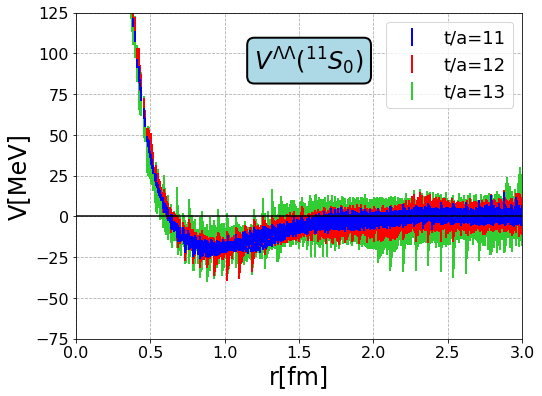
(a)

(b)

(c)

(d)

Figure 1: The $S$-wave coupled-channel $\Lambda\Lambda$-$N\Xi$ potential in ${{}^{11}S_{0}}$. The $V^{\Lambda\Lambda}$, $V^{\Lambda\Lambda}_{N\Xi}$, $V^{N\Xi}_{\ \Lambda\Lambda}$ and $V^{N\Xi}$ potentials are shown in (a), (b), (c) and (d), respectively.

In Fig. 1, the coupled channel potentials $V^{c}_{\ c^{\prime}}({{}^{11}S_{0}})(r)$ in the interval $11\leq t/a\leq 13$ are shown. (For the diagonal part ($c=c^{\prime}$), we omit the suffix $c^{\prime}$ for simplicity.) See Appendix A for the examples of wider range of $t/a$. Within the statistical errors, no significant $t$-dependence is found, which implies that the leading-order truncation of the derivative expansion is reasonable. The diagonal potentials, $V^{\Lambda\Lambda}$ and $V^{N\Xi}$ in Fig. 1 (a,d), have attractive pocket with a long-range tail together with a short-range repulsive core. From the meson exchange picture, the one-pion exchange is allowed only in $N\Xi$-$N\Xi$ channel. One interesting feature is that the overall attraction in $V^{N\Xi}$ is substantially larger than that in $V^{\Lambda\Lambda}$. The off-diagonal potentials shown in Fig. 1 (b,c) are found to be non-zero only at short distance, which suggests that the $\Lambda\Lambda$-$N\Xi$ coupling is weak at low energies.

(a)

(b)

(c)

Figure 2: The $S$-wave $N\Xi$ potentials in ${{}^{31}S_{0}}$, ${{}^{13}S_{1}}$, ${{}^{33}S_{1}}$ are plotted in (a), (b) and (c), respectively.

The $S$-wave $N\Xi$ potentials in the ${{}^{31}S_{0}}$, ${{}^{13}S_{1}}$ and ${{}^{33}S_{1}}$ states are shown in Fig. 2 (a), (b) and (c), respectively. Again, no significant $t$-dependence of the potentials is found in the interval $t/a=11-13$ within the statistical errors. Also, they have stronger repulsive core and weaker mid-range attraction than those in the ${{}^{11}S_{0}}$ $N\Xi$ potential.

(a)

(b)

(c)

(d)

Figure 3: The $S$-wave $N\Xi$ potentials in the operator basis: $V_{0}$, $V_{\sigma}$, $V_{\tau}$ and $V_{\sigma\tau}$ are shown in (a), (b), (c) and (d), respectively. The inset shows a zoom-up in the interval, $0.5\ {\rm fm}\leq r\leq 2.5\ {\rm fm}$.

To capture the strong spin and isospin dependence of the $N\Xi$ potentials, following decomposition with the operator basis is useful [28]

$$V(r)=V_{0}(r)+V_{\sigma}(r)(\vec{\sigma}_{1}\cdot\vec{\sigma}_{2})+V_{\tau}(r)(\vec{\tau}_{1}\cdot\vec{\tau}_{2})+V_{\sigma\tau}(r)(\vec{\sigma}_{1}\cdot\vec{\sigma}_{2})(\vec{\tau}_{1}\cdot\vec{\tau}_{2}).$$ (5)

This is equivalently rewritten as a relation between the spin-isospin basis and the operator basis;

$$\left(\begin{array}[]{c}V({{}^{11}S_{0}})(r)\\ V({{}^{31}S_{0}})(r)\\ V({{}^{13}S_{1}})(r)\\ V({{}^{33}S_{1}})(r)\end{array}\right)=\left(\begin{array}[]{cccc}1&-3&-3&9\\ 1&-3&1&-3\\ 1&1&-3&-3\\ 1&1&1&1\end{array}\right)\left(\begin{array}[]{c}V_{0}(r)\\ V_{\sigma}(r)\\ V_{\tau}(r)\\ V_{\sigma\tau}(r)\end{array}\right)\equiv\hat{A}\left(\begin{array}[]{c}V_{0}(r)\\ V_{\sigma}(r)\\ V_{\tau}(r)\\ V_{\sigma\tau}(r)\end{array}\right).$$ (22)

Shown in Fig. 3 are the $N\Xi$ potentials in the operator basis. The scalar part of the $N\Xi$ potential, $V_{0}^{N\Xi}$, have an attractive pocket at around $1.0$ fm as well as the short-range repulsion. The former may be related to the correlated two-pion exchange as in the case of the mid-range attraction in the $S$-wave $NN$ interactions. We also find that $V_{\sigma\tau}^{N\Xi}$ has a long-range attractive tail, which is consistent with the one-pion exchange picture.

5 Analytic forms of $\Lambda\Lambda$ and $N\Xi$ potentials

For phenomenological applications, it is useful to fit the LQCD potential in terms of a combination of simple analytic functions.

For the diagonal $\Lambda\Lambda$-$\Lambda\Lambda$ potential and the off-diagonal $\Lambda\Lambda$-$N\Xi$ potential in the ${{}^{11}S_{0}}$ channel shown in Fig. 1 (a,b), we consider the following fit functions,

$$V^{\Lambda\Lambda}(r) = \sum_{i=1}^{2}\alpha_{i}^{\Lambda\Lambda}e^{-\frac{r^{2}}{{\beta_{i}^{\Lambda\Lambda}}^{2}}}+\lambda_{2}^{\Lambda\Lambda}\left[{\cal{Y}}(\rho_{2}^{\Lambda\Lambda},m_{\pi},r)\right]^{2},$$ (23)

$$V^{\Lambda\Lambda}_{N\Xi}(r) = \sum_{i=1}^{2}\alpha_{i}e^{-\frac{r^{2}}{{\beta_{i}}^{2}}}+\lambda_{1}{\cal{Y}}(\rho_{1},m_{K},r),$$ (24)

where the Yukawa function with a form factor ${\cal{Y}}$ is defined as

$${\cal{Y}}(\rho,m,r)\equiv\left(1-e^{-\frac{r^{2}}{\rho^{2}}}\right)\frac{e^{-mr}}{r}.$$ (25)

In Eqs. (23,24), the Gauss functions describe the short range part of the potential, while the Yukawa functions are motivated by the meson exchange picture at medium and long range distances. In particular, the squared Yukawa function in eq. (23) represents the two-pion process in the $\Lambda\Lambda-\Lambda\Lambda$ interaction whose long-range part does not exchange isospin and strangeness. Similarly, the Yukawa function in eq. (24) represents the longest range single-kaon process in the $\Lambda\Lambda-N\Xi$ transition. Note that the kaon and pion masses $m_{K}$ and $m_{\pi}$ are fixed to be the measured values on the lattice, $525$ MeV and $146$ MeV, respectively.

As for the fitting to the $N\Xi$ potentials in Fig. 1 (d) and Fig. 2 (a,b,c), we consider the following analytic form;

$$V(C)(r)=\sum_{i=1}^{3}\alpha_{i}(C)e^{-\frac{r^{2}}{{\beta_{i}}^{2}}}+\lambda_{2}(C)\left[{\cal{Y}}(\rho_{2},m_{\pi},r)\right]^{2}+\lambda_{1}(C){\cal{Y}}(\rho_{1},m_{\pi},r),$$ (26)

with $C$ being ${{}^{11}S_{0}}$, ${{}^{31}S_{0}}$, ${{}^{13}S_{1}}$ or ${{}^{33}S_{1}}$. The range parameters $\beta_{1,2,3}$ and $\rho_{1,2}$ for $N\Xi$ potentials are assumed to be independent of $C$. The above form is motivated by the following analytic forms in the operator basis where the one-pion and two-pion exchange contributions are singled out explicitly in $V_{\sigma\tau}$ and $V_{0}$, respectively;

$$V_{0}(r) = \sum_{i=1}^{3}\alpha_{i}^{(0)}e^{-\frac{r^{2}}{{\beta_{i}}^{2}}}+\lambda_{2}^{(0)}\left[{\cal{Y}}(\rho_{2},m_{\pi},r)\right]^{2}$$

$$V_{\sigma}(r) = \sum_{i=1}^{3}\alpha_{i}^{(\sigma)}e^{-\frac{r^{2}}{{\beta_{i}}^{2}}},\ \ \ V_{\tau}(r)=\sum_{i=1}^{3}\alpha_{i}^{(\tau)}e^{-\frac{r^{2}}{{\beta_{i}}^{2}}}$$

$$V_{\sigma\tau}(r) = \sum_{i=1}^{3}\alpha_{i}^{(\sigma\tau)}e^{-\frac{r^{2}}{{\beta_{i}}^{2}}}+\lambda_{1}^{(\sigma\tau)}{\cal{Y}}(\rho_{1},m_{\pi},r).$$ (27)

The relation between the parameters are imposed as

$$\left(\begin{array}[]{c}\alpha_{i}({{}^{11}S_{0}})\\ \alpha_{i}({{}^{31}S_{0}})\\ \alpha_{i}({{}^{13}S_{1}})\\ \alpha_{i}({{}^{33}S_{1}})\end{array}\right)=\hat{A}\left(\begin{array}[]{c}\alpha_{i}^{(0)}\\ \alpha_{i}^{(\sigma)}\\ \alpha_{i}^{(\tau)}\\ \alpha_{i}^{(\sigma\tau)}\end{array}\right),\hskip 8.53581pt\left(\begin{array}[]{ccc}\lambda_{1}({{}^{11}S_{0}})\\ \lambda_{1}({{}^{31}S_{0}})\\ \lambda_{1}({{}^{13}S_{1}})\\ \lambda_{1}({{}^{33}S_{1}})\end{array}\right)=\left(\begin{array}[]{c}9\lambda_{1}^{(\sigma\tau)}\\ -3\lambda_{1}^{(\sigma\tau)}\\ -3\lambda_{1}^{(\sigma\tau)}\\ \lambda_{1}^{(\sigma\tau)}\end{array}\right),$$ (44)

and $\lambda_{2}(C)=\lambda_{2}^{(0)}$ being independent of the channel, $C$.

It is in order here to mention about the fitting procedure of the off-diagonal $\Lambda\Lambda$-$N\Xi$ potential. Although there is nothing wrong to solve the coupled-channel Schrödinger equation with non-Hermitian potential, it is customary to use Hermitian potential in phenomenological studies in nuclear physics. Since the difference between $V^{\Lambda\Lambda}_{N\Xi}$ and $V^{N\Xi}_{\Lambda\Lambda}$ are confined only at short distances if any (see Fig. 1 (b,c)), it does not affect the low-energy scattering observables. We have checked this explicitly by choosing an Hermitian potential with the off-diagonal part is taken either $V^{\Lambda\Lambda}_{N\Xi}$, $V^{N\Xi}_{\Lambda\Lambda}$ or their average $\bar{V}^{\Lambda\Lambda}_{N\Xi}=(V^{\Lambda\Lambda}_{N\Xi}+V^{N\Xi}_{\Lambda\Lambda})/2$. As shown in B, the phase shifts in these three cases do not have difference within the statistical errors. Therefore, in the following we show the fit parameters corresponding to $\bar{V}^{\Lambda\Lambda}_{N\Xi}$.

Final fit parameters are given in Table 2 for $V^{\Lambda\Lambda}({{}^{11}S_{0}})$ and Table 3 for $\bar{V}^{\Lambda\Lambda}_{N\Xi}({{}^{11}S_{0}})$, with three different values $t/a=11,12,13$. Also shown in Table 4 are those for $V^{N\Xi}$ in ${{}^{11}S_{0}}$, ${{}^{31}S_{0}}$, ${{}^{13}S_{1}}$ and ${{}^{33}S_{1}}$ channels with $t/a=11,12,13$, where the data in all $N\Xi$ channels are fitted simultaneously. We perform uncorrelated fit for the potential, where the fit range is taken to be $r=[0,2]$ fm independent of the potentials so that there are 220 coordinate data points to be fitted in each channel. For convenience, we show the corresponding parameters for $V^{N\Xi}$ in the operator basis in Table 1. As for the choice of these $t/a$, see A.

Table 2: Fitted parameters for $V^{\Lambda\Lambda}({{}^{11}S_{0}})$ with statistical errors using the data for $r=[0,2]$fm. $\alpha_{i}$, $\beta_{i}$ and $\rho_{i}$ are given in units of [MeV], [fm] and [fm], respectively. $\lambda_{1}$ and $\lambda_{2}$ are given in units of [MeV $\cdot$ fm] and [MeV $\cdot$ fm²], respectively. The values of $\chi^{2}$/d.o.f. with #d.o.f = $214$ are $1.30(40)$, $0.76(18)$ and $0.74(30)$ for $t/a=11$, $12$ and $13$, respectively.

	Gauss-1		Gauss-2		[Yukawa]2
$t/a$	$\alpha_{1}^{\Lambda\Lambda}$	$\beta_{1}^{\Lambda\Lambda}$	$\alpha_{2}^{\Lambda\Lambda}$	$\beta_{2}^{\Lambda\Lambda}$	$\lambda_{2}^{\Lambda\Lambda}$	$\rho_{2}^{\Lambda\Lambda}$
$11$	1466.4(28.4)	0.160(5)	407.1(43.9)	0.366(18)	-170.3(32.2)	0.918(87)
$12$	1486.7(46.5)	0.156(7)	418.2(64.6)	0.367(25)	-160.0(50.8)	0.929(148)
$13$	1338.0(89.5)	0.143(10)	560.7(124.2)	0.322(27)	-176.2(114.9)	1.033(292)

Table 3: Fitted parameters for the transition potential $\bar{V}^{\Lambda\Lambda}_{N\Xi}({{}^{11}S_{0}})$ with the statistical errors using the data for $r=[0,2]$fm. Units are the same as those in Table 2. The values of $\chi^{2}$/d.o.f. with #d.o.f = $214$ are $1.24(35)$, $1.01(28)$ and $1.13(28)$ for $t/a=11$, $12$ and $13$, respectively.

	Gauss-1		Gauss-2		Yukawa
$t/a$	$\alpha_{1}$	$\beta_{1}$	$\alpha_{2}$	$\beta_{2}$	$\lambda_{1}$	$\rho_{1}$
$11$	1228.0(21.9)	0.187(7)	294.9(16.6)	0.433(16)	-69.7(16.2)	0.130(8)
$12$	1206.7(27.0)	0.191(12)	307.4(30.3)	0.438(25)	-75.2(26.9)	0.133(13)
$13$	1252.7(47.6)	0.187(25)	306.9(46.4)	0.428(58)	-65.8(58.1)	0.128(28)

Table 4: Fitted parameters for $V^{N\Xi}$ $({{}^{11}S_{0}},{{}^{31}S_{0}},{{}^{13}S_{1}},{{}^{33}S_{1}})$ with the statistical errors using the data for $r=[0,2]$fm. In the last column, $\lambda_{2}(C)$ is independent of the channel, $C$. Units are the same as those in Table 2. For the corresponding parameters in the operator basis, see Table 1. The values of $\chi^{2}$/d.o.f. with #d.o.f = 861 are $2.34(39)$, $1.38(21)$ and $1.28(18)$ for $t/a=11$, $12$ and $13$, respectively.

	Gauss-1	Gauss-2	Gauss-3	Yukawa	[Yukawa]2
$t/a=11$	$\alpha_{1}$	$\alpha_{2}$	$\alpha_{3}$	$\lambda_{1}$	$\lambda_{2}$
${{}^{11}S_{0}}$	40.2(36.1)	51.5(28.2)	30.5(14.9)	-14.6(1.6)	-109.8(7.9)
${{}^{31}S_{0}}$	1766.1(75.6)	920.3(56.8)	240.5(31.1)	4.9(5)	-109.8(7.9)
${{}^{13}S_{1}}$	493.3(30.9)	300.8(22.9)	92.0(17.3)	4.9(5)	-109.8(7.9)
${{}^{33}S_{1}}$	944.8(46.8)	568.6(29.8)	190.3(25.0)	-1.6(2)	-109.8(7.9)
	$\beta_{1}$	$\beta_{2}$	$\beta_{3}$	$\rho_{1}$	$\rho_{2}$
	0.129(3)	0.258(12)	0.569(21)	0.249(38)	0.609(23)

	Gauss-1	Gauss-2	Gauss-3	Yukawa	[Yukawa]2
$t/a=12$	$\alpha_{1}$	$\alpha_{2}$	$\alpha_{3}$	$\lambda_{1}$	$\lambda_{2}$
${{}^{11}S_{0}}$	-81.3(54.3)	171.1(59.1)	4.9(27.3)	-12.8(2.2)	-97.3(9.6)
${{}^{31}S_{0}}$	1677.2(90.1)	991.3(62.7)	290.8(43.2)	4.3(7)	-97.3(9.6)
${{}^{13}S_{1}}$	449.2(52.5)	348.9(31.8)	110.3(22.3)	4.3(7)	-97.3(9.6)
${{}^{33}S_{1}}$	849.5(53.4)	653.9(32.7)	210.8(35.9)	-1.4(2)	-97.3(9.6)
	$\beta_{1}$	$\beta_{2}$	$\beta_{3}$	$\rho_{1}$	$\rho_{2}$
	0.124(3)	0.241(12)	0.533(22)	0.136(22)	0.603(48)

	Gauss-1	Gauss-2	Gauss-3	Yukawa	[Yukawa]2
$t/a=13$	$\alpha_{1}$	$\alpha_{2}$	$\alpha_{3}$	$\lambda_{1}$	$\lambda_{2}$
${{}^{11}S_{0}}$	62.4(125.4)	-43.6(144.7)	123.8(110.2)	-12.5(2.4)	-83.5(14.6)
${{}^{31}S_{0}}$	1599.4(308.3)	879.8(324.3)	496.7(136.8)	4.2(8)	-83.5(14.6)
${{}^{13}S_{1}}$	345.5(106.5)	287.0(153.7)	268.9(120.9)	4.2(8)	-83.5(14.6)
${{}^{33}S_{1}}$	836.0(163.3)	487.2(213.1)	383.1(125.2)	-1.4(3)	-83.5(14.6)
	$\beta_{1}$	$\beta_{2}$	$\beta_{3}$	$\rho_{1}$	$\rho_{2}$
	0.124(10)	0.228(34)	0.499(33)	0.307(307)	0.417(74)

The analytic forms of the potential, Eqs. (23), (24) and (26), together with the parameters in Table 2-4 are useful for phenomenological applications such as the calculation of the scattering phase shifts (as given in Fig. 4 and Fig. 5) and also the calculation of the binding energy of $\Xi$ hypernuclei (as discussed in ref.[31]). The diagonal potentials (Fig.1(a), Fig.1(d) and Fig.2) are composed of the short-range part (parametrized by $\alpha_{i}$ and $\beta_{i}$) and the medium/long range part (parametrized by $\lambda_{i}$, $\rho_{i}$). The positive values of $\alpha_{i}$ correspond to short-range repulsion, while the negative values of $\lambda_{i}$ correspond to medium/long range attraction.

6 Scattering observables

The $\Lambda\Lambda$ and $N\Xi$ coupled-channel scattering phase shifts in the ${{}^{11}S_{0}}$ channel are calculated by solving the coupled-channel Schrödinger equation in the infinite volume with the fitted potentials given in the previous section. Since we consider low-energy scatterings, we adopt the non-relativistic kinematics hereafter.

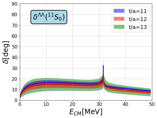
(a)

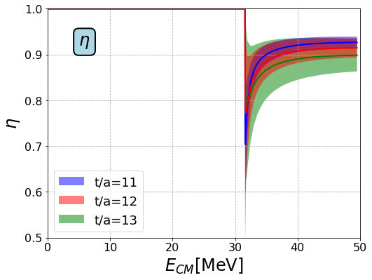
(b)

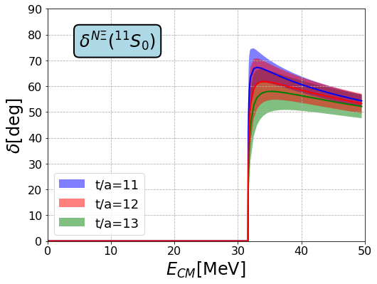
(c)

Figure 4: (a) $\Lambda\Lambda$ scattering phase shift, (b) $\Lambda\Lambda$ inelasticity, and (c) $N\Xi$ scattering phase shift in the ${{}^{11}S_{0}}$ channel.

The $\Lambda\Lambda$ phase shifts and the inelasticity are defined by the $\Lambda\Lambda$-component of the two-by-two S-matrix, $({\bf S})_{\Lambda\Lambda}=\eta\exp(2i\delta_{\Lambda\Lambda})$. In Fig. 4 (a,b), they are shown as a function of the center-of-mass energy $E_{\rm CM}=k^{2}/m_{\Lambda}$ with $k$ being the relative momentum between $\Lambda$s for $t/a=11,12,13$. The $t$-dependence is minor within the statistical errors. We found that $\Lambda\Lambda$ attraction is rather weak, as inferred from Fig. 1 (a). Accordingly, no bound or resonant di-hyperon exits around the $\Lambda\Lambda$ threshold in (2+1)-flavor QCD at nearly physical quark masses. This is in contrast to the case of a possible $H$-dibaryon in 3-flavor QCD at heavy quark masses [29, 30].

Low-energy part of $\Lambda\Lambda$ phase shifts in Fig. 4 (a) provides the scattering length and the effective range using the $S$-wave effective range expansion (ERE) formula,

$$k\cot\delta=-\frac{1}{a_{0}}+\frac{1}{2}r_{\rm{eff}}k^{2}+{\cal{O}}(k^{4}),$$ (45)

where we use the sign convention of $a_{0}$ in nuclear and atomic physics. The results are

$$a_{0}^{(\Lambda\Lambda)}=-0.81\pm 0.23{{}^{+0.00}_{-0.13}}\ [{\rm{fm}}],\hskip 10.00002ptr^{(\Lambda\Lambda)}_{\rm{eff}}=5.47\pm 0.78{{}^{+0.09}_{-0.55}}\ [{\rm{fm}}],$$ (46)

where the central values and the statistical errors are estimated at $t/a=12$, while the systematic errors are estimated from the central values for $t/a=11$ and $13$. For comparison, the experimental neutron-neutron ERE parameters are $(a_{0}^{(nn)},r^{(nn)}_{\rm{eff}})=(-18.5,2.80)$ fm. Our results in Eq. (46) were recently confirmed to be consistent with a constraint obtained from the $\Lambda\Lambda$ momentum correlation of in p-p and p-Pb collisions [8]. (Note that the sign convention of $a_{0}$ in [8] is defined to be opposite from ours.)

We note that the $\Lambda\Lambda$ phase shift in Fig. 4 (a) and the inelasticity $\eta$ in Fig. 4 (b) near the $N\Xi$ threshold, show a sharp enhancement and a rapid drop and show an enhancement, respectively, due to the off-diagonal coupling. Also, Fig. 4 (c) shows a sharp increase of the $N\Xi$ phase shift $\delta^{N\Xi}$ up to about $60^{\circ}$ just above the $N\Xi$ threshold, which indicates a significant $N\Xi$ attraction in the ${{}^{11}S_{0}}$ channel. Indeed, we have confirmed that the $N\Xi$ system is in the unitary region and a virtual pole is created in the ${{}^{11}S_{0}}$ channel.

(a)

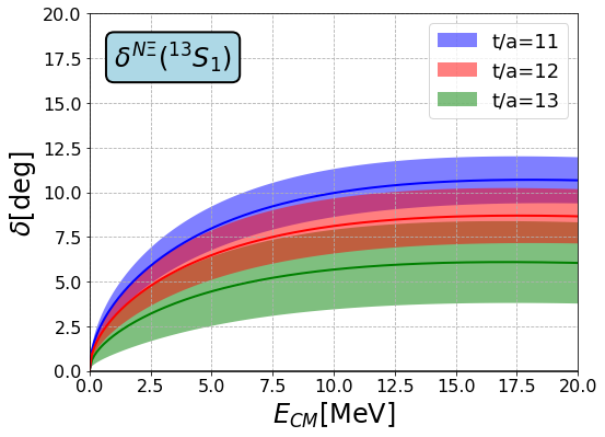
(b)

(c)

Figure 5: The $N\Xi$ scattering phase shifts in ${{}^{31}S_{0}}$, ${{}^{13}S_{1}}$ and ${{}^{33}S_{1}}$ are shown in (a), (b) and (c), respectively.

The $S$-wave $N\Xi$ scattering phase shifts in ${{}^{31}S_{0}}$, ${{}^{13}S_{1}}$ and ${{}^{33}S_{1}}$ channel are shown in Fig. 5 as a function of $E_{\rm CM}=k^{2}\times(1/(2m_{N})+1/(2m_{\Xi}))$. We find that the interaction in the ${{}^{31}S_{0}}$ channel is weakly repulsive while the ${{}^{13}S_{1}}$ and ${{}^{33}S_{1}}$ channels are weakly attractive, at low energies.

7 Summary and conclusion remarks

We have studied strangeness ${\cal{S}}=-2$ baryon-baryon interactions focusing on the $S$-wave $\Lambda\Lambda$ and $N\Xi$ potentials using the (2+1)-flavor lattice QCD configurations at the almost physical point ($m_{\pi}\simeq 146{\rm{MeV}}$ and $m_{K}\simeq 525{\rm{MeV}}$) analyzed by the coupled-channel HAL QCD method. Resultant lattice QCD potentials in different isospin-spin channels (${{}^{11}S_{0}}$, ${{}^{31}S_{0}}$, ${{}^{13}S_{1}}$ and ${{}^{33}S_{1}}$) are parametrized by analytic functions (a combination of Gaussian and Yukawa forms) for calculating the scattering observables such as the phase shift and inelasticity.

We found that $\Lambda\Lambda$ (${{}^{11}S_{0}}$) has attraction at low-energies, while it is not strong enough to generate bound or resonant dihyperon around the $\Lambda\Lambda$ threshold. Our scattering length and the effective range in Eq. (46) were recently confirmed to be consistent with an experimental constraint by ALICE experiment at LHC [8]. On the other hand, we found that the $N\Xi({{}^{11}S_{0}}$) has relatively a strong attraction to drive the system into the unitary regime, while $N\Xi({{}^{31}S_{0}}$) is weakly repulsive and $N\Xi({{}^{13}S_{1}})$ and $N\Xi({{}^{33}S_{1}})$ are weakly attractive. These features may lead to a light $\Xi$ hypernuclei as recently discussed in [31]. Also, they introduce an attractive momentum correlation between proton and $\Xi^{-}$ on top of the Coulomb attraction as suggested in [32] and confirmed recently by ALICE experiment at LHC [9].

There remain several future problems to be solved. First of all, we need to carry out (2+1)-flavor and (1+1+1)-flavor lattice simulations exactly at the physical point to check whether the virtual pole in the $N\Xi({{}^{11}S_{0}}$) channel turns into a resonance below the $N\Xi$ threshold. Another issue is to carry out full channel coupling analysis with $\Lambda\Sigma$ and $\Sigma\Sigma$ to cover the scattering energy beyond the $\Lambda\Sigma$ threshold.

Appendix A $t$-dependence of $N\Xi$ potentials

Fig. 1 shows the $t$-dependence of $S$-wave $N\Xi$ potentials in the range $t/a=9$ to $15$ which is wider than that used in the text. Overall stability of the results in this wider range of $t/a$ can be seen within the statistical error bars. Nevertheless, we find that the fitting by analytic functions in Sec. 5 is rather unstable against at short time (e.g. $t/a\leq 10$) probably due to the inelastic state contaminations. Also the large statistical errors prevent us to extract sensible fit parameters for $t/a\geq 14$. This is why we chose the optimal range $11\leq t/a\leq 13$ throughout this paper.

(a)

(b)

(c)

(d)

Figure 1: The $t$-dependence of $S$-wave $N\Xi$ potentials. The $V^{N\Xi}({{}^{11}S_{0}})$, $V^{N\Xi}({{}^{31}S_{0}})$, $V^{N\Xi}({{}^{13}S_{1}})$ and $V^{N\Xi}({{}^{33}S_{1}})$ are shown in (a), (b), (c) and (d), respectively.

Appendix B Dependence on different off-diagonal potentials

To check the observable difference among three choices of the off-diagonal part of the Hermitian potential ($V^{\Lambda\Lambda}_{N\Xi}$, $V^{N\Xi}_{\Lambda\Lambda}$ and their average $\bar{V}^{\Lambda\Lambda}_{N\Xi}$), the $\Lambda\Lambda$ scattering phase shifts and the $N\Xi$ scattering phase shifts are shown in Fig. 1 and in Fig. 2, respectively. Within the statistical errors, three results are consistent with each other for all $t/a$ used in this paper. Thus we consider $\bar{V}^{\Lambda\Lambda}_{N\Xi}$ in the text.

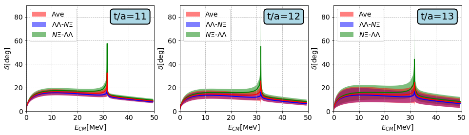
Figure 1: The $\Lambda\Lambda$ scattering phase shifts for $t/a=11$ (left), $t/a=12$ (middle) and $t/a=13$ (right). Blue, green and red curves correspond to the phase shifts calculated with $V^{\Lambda\Lambda}_{N\Xi}$, $V^{N\Xi}_{\Lambda\Lambda}$ and $\bar{V}^{\Lambda\Lambda}_{N\Xi}$, respectively.

Figure 2: Same with Fig. 1 but for $N\Xi$ scattering phase shifts.

Appendix C Fit parameters of $N\Xi$ potentials in the operator basis

We show the fit parameters of $N\Xi$ potentials in the operator basis, $\left(V_{0},V_{\sigma},V_{\tau},V_{\sigma\tau}\right)$ given in Eq. (5). For parameters in the spin-isospin basis, see Table 4.

Table 1: Fitting parameters for $V^{N\Xi}$ in the operator basis with the statistical errors. Units are the same as those in Table 4.

	Gauss-1	Gauss-2	Gauss-3	Yukawa	[Yukawa]2
$t/a=11$	$\alpha_{1}$	$\alpha_{2}$	$\alpha_{3}$	$\lambda_{1}$	$\lambda_{2}$
$V_{0}$	957.6(44.7)	552.0(29.3)	171.3(23.6)	—	-109.8(7.9)
$V_{\sigma}$	-125.7(8.3)	-50.4(6.5)	-5.6(1.6)	—	—
$V_{\tau}$	192.5(9.9)	104.5(8.0)	31.6(3.1)	—	—
$V_{\sigma\tau}$	-79.6(2.7)	-37.6(2.8)	-7.0(0.9)	-1.6(2)	—
	$\beta_{1}$	$\beta_{2}$	$\beta_{3}$	$\rho_{1}$	$\rho_{2}$
	0.129(3)	0.258(12)	0.569(21)	0.249(38)	0.609(23)

	Gauss-1	Gauss-2	Gauss-3	Yukawa	[Yukawa]2
$t/a=12$	$\alpha_{1}$	$\alpha_{2}$	$\alpha_{3}$	$\lambda_{1}$	$\lambda_{2}$
$V_{0}$	871.4(54.6)	629.8(33.0)	194.1(33.0)	—	-97.3(9.6)
$V_{\sigma}$	-122.0(9.3)	-52.2(8.9)	-8.4(2.7)	—	—
$V_{\tau}$	185.0(10.0)	108.5(7.2)	36.7(5.2)	—	—
$V_{\sigma\tau}$	-84.9(5.7)	-32.2(5.4)	-11.6(1.6)	-1.4(2)	—
	$\beta_{1}$	$\beta_{2}$	$\beta_{3}$	$\rho_{1}$	$\rho_{2}$
	0.124(3)	0.241(12)	0.533(22)	0.136(22)	0.603(48)

	Gauss-1	Gauss-2	Gauss-3	Yukawa	[Yukawa]2
$t/a=13$	$\alpha_{1}$	$\alpha_{2}$	$\alpha_{3}$	$\lambda_{1}$	$\lambda_{2}$
$V_{0}$	838.9(158.0)	490.1(206.4)	366.8(123.9)	—	-83.5(14.6)
$V_{\sigma}$	-125.4(27.1)	-53.0(24.1)	-12.2(4.4)	—	—
$V_{\tau}$	188.0(40.5)	95.2(36.6)	44.7(8.4)	—	—
$V_{\sigma\tau}$	-65.4(20.6)	-45.2(17.2)	-16.2(4.7)	-1.4(3)	—
	$\beta_{1}$	$\beta_{2}$	$\beta_{3}$	$\rho_{1}$	$\rho_{2}$
	0.124(10)	0.228(34)	0.499(33)	0.307(307)	0.417(74)

References

- [1] R. L. Jaffe, Phys. Rev. Lett. 38 (1977) 195 [Erratum-ibid. 38 (1977) 617].
- [2] T. Sakai, K. Shimizu and K. Yazaki, Prog. Theor. Phys. Suppl. 137 (2000) 121 [nucl-th/9912063].
- [3] B. H. Kim et al. [Belle Collaboration], Phys. Rev. Lett. 110 (2013) 222002 [arXiv:1302.4028 [hep-ex]].
- [4] K. Nakazawa et al., PTEP 2015 (2015) 033D02.
- [5] A. Gal, E. V. Hungerford, and D. J. Millener, Rev. Mod. Phys. 88 (2016) 035004.
- [6] E. Hiyama and K. Nakazawa, Ann. Rev. Nucl. Part. Sci. 68 (2018) 131.
- [7] Adamczyk et al. [STAR collaboration], Phys. Rev. Lett. 114 (2015) 022301.
-
[8]
S. Acharya et al. [ALICE Collaboration],
Phys. Rev. C 99, 024001 (2019) [arXiv:1805.12455 [nucl-ex]];
Phys. Lett. B 797, 134822 (2019) [arXiv:1905.07209 [nucl-ex]]. - [9] S. Acharya et al. [ALICE Collaboration], Phys. Rev. Lett. 123 (2019) 112002 [arXiv:1904.12198 [nucl-ex]].
- [10] N. Ishii, S. Aoki and T. Hatsuda, Phys. Rev. Lett. 99 (2007) 022001 [nucl-th/0611096].
- [11] S. Aoki, T. Hatsuda and N. Ishii, Prog. Theor. Phys. 123 (2010) 89 [arXiv:0909.5585 [hep-lat]].
- [12] N. Ishii et al. [HAL QCD Collaboration], Phys. Lett. B 712 (2012) 437 [arXiv:1203.3642 [hep-lat]].
- [13] S. Aoki et al. [HAL QCD Collaboration], Proc. Japan Acad. B 87 (2011) 509 [arXiv:1106.2281 [hep-lat]].
- [14] S. Aoki, B. Charron, T. Doi, T. Hatsuda, T. Inoue and N. Ishii, Phys. Rev. D 87 (2013) 034512 [arXiv:1212.4896 [hep-lat]].
- [15] K. Sasaki et al. [HAL QCD Collaboration], PTEP 2015 (2015) 113B01 [arXiv:1504.01717 [hep-lat]].
- [16] T. Iritani et al. [HAL QCD Collaboration], Phys. Lett. B 792 (2019) 284 [arXiv:1810.03416 [hep-lat]].
- [17] S. Gongyo et al., Phys. Rev. Lett. 120 (2018) 212001 [arXiv:1709.00654 [hep-lat]].
- [18] T. Iritani et al. [HAL QCD Collaboration], Phys. Rev. D 99 (2019) 014514 [arXiv:1805.02365 [hep-lat]].
- [19] T. Iritani et al. [HAL QCD Collaboration], JHEP 1903 (2019) 007 [arXiv:1812.08539 [hep-lat]].
- [20] K.-I. Ishikawa et al. [PACS Collaboration], PoS LATTICE 2015 (2016) 075 [arXiv:1511.09222 [hep-lat]].
- [21] K. I. Ishikawa et al. [PACS Collaboration], Phys. Rev. D 98 (2018) 074510 [arXiv:1807.03974 [hep-lat]].
- [22] T. Boku et al., PoS LATTICE 2012 (2012) 188 [arXiv:1210.7398 [hep-lat]].
- [23] M. Terai, K. I. Ishikawa, Y. Sugisaki, K. Minami, F. Shoji, Y. Nakamura, Y. Kuramashi, M. Yokokawa, IPSJ Transactions on Advanced Computing Systems, Vol.6 No.3 43-57 (Sep. 2013) (in Japanese).
- [24] Y. Nakamura, K.-I. Ishikawa, Y. Kuramashi, T. Sakurai and H. Tadano, Comput. Phys. Commun. 183 (2012) 34 [arXiv:1104.0737 [hep-lat]].
- [25] Y. Osaki and K. I. Ishikawa, PoS LATTICE 2010 (2010) 036 [arXiv:1011.3318 [hep-lat]].
- [26] T. Doi and M. G. Endres, Comput. Phys. Commun. 184 (2013) 117 [arXiv:1205.0585 [hep-lat]].
- [27] H. Nemura, Comput. Phys. Commun. 207 (2016) 91 [arXiv:1510.00903 [hep-lat]].
- [28] S. Okubo and R. E. Marshak, Ann. of Phys. 4 (1958)166.
-
[29]
T. Inoue et al. [HAL QCD Collaboration],
Prog. Theor. Phys. 124 (2010) 591 [arXiv:1007.3559 [hep-lat]];
Phys. Rev. Lett. 106 (2011) 162002 [arXiv:1012.5928 [hep-lat]];
Nucl. Phys. A 881 (2012) 28 [arXiv:1112.5926 [hep-lat]]. - [30] S. R. Beane et al. [NPLQCD Collaboration], Phys. Rev. Lett. 106 (2011) 162001 [arXiv:1012.3812 [hep-lat]].
- [31] E. Hiyama, K. Sasaki, T. Miyamoto, T. Doi, T. Hatsuda, Y. Yamamoto and T. A. Rijken, Phys. Rev. Lett. 124 (2020) no.9, 092501 [arXiv:1910.02864 [nucl-th]].
- [32] T. Hatsuda, K. Morita, A. Ohnishi and K. Sasaki, Nucl. Phys. A 967 (2017) 856 [arXiv:1704.05225 [nucl-th]].
- [33] International Lattice Data Grid (ILDG), (Available at:http://plone.jldg.org/ ).
- [34] Japan Lattice Data Grid (JLDG), (Available at:http://www.jldg.org/ ).
- [35] T. Amagasa, et al., J. Phys. Conf. Ser. 664 (2015) 042058.
- [36] M. Schröck and H. Vogt, Comput. Phys. Commun. 184 (2013) 1907 [arXiv:1212.5221 [hep-lat]].