Faster-Than-Light Solitons in $1+1$ Dimensions

Abstract

The existence of a faster-than-light particle is in direct opposition to Einstein’s relativity and the principle of causality. However, we show that the theory of classical relativistic fields is not inherently inconsistent with the existence of the faster-than-light particle-like soliton solutions in $1+1$ dimensions. We introduce two extended KG models ($k$-fields) that lead to a zero-energy and a nonzero-energy stable particle-like solution with faster-than light speeds, respectively.

Keywords : non-topological soliton, faster than light particle, solitary wave solution, nonlinear Klein-Gordon equation, $k$-field.

1 Introduction

The typical and classical conception assumes that a particle is a stable entity that may be found at any arbitrary velocity. In the context of the relativistic classical field theory, such stable particle-like solutions with localized energy density functions are called solitons [1, 2, 3, 4]. In many respects, they resemble the real stable particles. For example, they satisfy the same well-known relativistic energy-momentum relations of special relativity and their dimension would contract in the direction of motion according to the Lorentz contraction law. There are many works on relativistic solitons and solitary wave solutions, among which one can mention the kink (anti-kink) solutions of the real nonlinear Klein-Gordon (KG) systems in $1+1$ dimensions [5, 6, 7, 8, 9, 10, 11, 12, 13, 14, 15, 16, 17, 18, 19, 20, 21, 22, 23, 24, 25], the Q-ball solutions of the complex nonlinear KG systems [26, 27, 28, 29, 30, 31, 32, 33, 34, 35, 36, 37, 38, 40, 39, 41], the Skyrme’s model [4, 42, 43, 44, 45] of baryons, and ’t Hooft Polyakov’s model which yields monopole soliton solutions [1, 4, 46, 47, 48, 49, 50].

Solitary wave solutions and solitons can be divided into two groups, topological and non-topological, depending on how they are at the boundaries. The topological solitons do not have the same behavior at far distances (boundaries) and are inevitably stable. Apart from Q-balls, the other cases mentioned above are topological solitons. However, the non-topological solitary wave solutions have the same boundary behaviors and are not necessarily stable. If we do not restrict ourselves to the relativistic field systems, the study of non-topological soliton solutions in several branches of physics and mathematics has been of great interest, for example, one can mention [51, 52, 53, 54, 55, 56, 57, 58, 59, 60, 61, 62].

According to the special theory of relativity, the motion of any matter particle is restricted to be at speeds less than the speed of light. However, for first time, the hypothetical faster-than-light (FTL) particles concept, was proposed by Gerald Feinberg who coined the term tachyons [63, 64] and defined them as the quanta of a special relativistic quantum field theory with imaginary mass. The complex speeds open up another possibility to build a theory with hypothetical particles at FTL speeds [65]. There are some notable works on this matter, which can be useful for the interested reader [66, 67]. For the hypothetical FTL particles, the main implication is the violation of causality, which is accepted as an obvious principle in physics. Thus, FTL particles may be discussed in theory and mathematics, but in the real world, the existence of such particles contradicts the accepted axioms. It is well known that in contrast to group velocity, phase velocities can easily exceed the speed of light.

In classical relativistic field theory with solitons solutions, there have not been introduced a special system so far, which yields a solitary wave or soliton solution at FTL speeds. In this paper, we show mathematically how a classical relativistic field theory can lead to a non-topological soliton solution at FTL speeds in $1+1$ dimensions. Here, the speed of light is ordinarily a limiting speed for the motion of the soliton solution, that is it cannot move at speeds less than the speed of light. In fact, two extended KG models will be introduced which yields zero and non-zero energy FTL soliton solutions, respectively. These models can be considered as toy mathematical models to show that the theory of relativistic classical fields is not inherently inconsistent with the existence of FTL particle-like solutions.

The extended KG systems or the so-called $k$-fields, have Lagrangian densities which are not linear in the kinetic scalar terms ${\cal S}_{ij}={\cal S}_{ji}=\partial_{\mu}\phi_{i}\partial^{\mu}\phi_{j}$ [68, 69, 70, 71, 72, 73, 74, 75]. Such Lagrangian densities can be also called non-canonical Lagrangian (NCL) densities [76, 77, 78, 79, 80, 81]. The solitary wave and soliton solutions of such systems are known as defect structures [68, 69, 70]. There are many works which deal with such systems with defect structures (e.g., domain walls, vortices and monopoles), among which one can mention [68, 69, 70, 82, 83]. In cosmology, the models with $k$-fields have become especially popular. They are suggested in the context of inflation leading to $k$-inflation [84, 85, 86], or they are used for describing dark energy and dark matter [87, 34, 88, 89, 90].

The organization of this paper is as follows: In Section 2, we will introduce a standard nonlinear KG system with an unstable FTL solitary wave solution. In Section 3, zero energy solitary wave solutions are introduced first, then an extended KG will be introduced with an energetically stable zero-energy soliton solution at FTL speeds. In section 4, by combining these two models, we will introduce a new system that leads to a stable FTL solitary wave solution with nonzero-energy. The last section is devoted to summary and conclusion.

2 An unstable solitary wave solution at FTL speeds

In the standard relativistic theory of the classical fields, it is common to start with a proper Lagrangian density and then try to find its solitary wave solutions. There is another approach where one can first consider a special proposed solitary wave solution and then try to find a proper Lagrangian density for it [23]. A solitary wave solution is a special solution that has a localized energy density function. For example, based on the second approach, for a real scalar field $\varphi$, we can consider a nonlinear KG Lagrangian density,

$${\cal L}=\partial^{\mu}\varphi\partial_{\mu}\varphi-U(\varphi)=\dot{\varphi}-\varphi^{\prime}-U(\varphi),$$ (1)

which is assumed to have a special localized Gaussian solution at rest in the following form:

$$\varphi_{o}=\exp(-x^{2}).$$ (2)

Here $U(\varphi)$ is called the field potential and should be determined in such a way that Eq. (2) becomes a special solution of the Lagrangian density (1). Note that, in Eq. (1), the dot (prime) indicates the time (space) derivative, and for the sake of simplicity, throughout the paper, we assume the speed of light to be equal to one. In fact, Eq. (2) is considered to be a special solution of the dynamical equation, which results from the Lagrangian density (1):

$$\Box\varphi=\frac{\partial^{2}\varphi}{\partial t^{2}}-\frac{\partial^{2}\varphi}{\partial x^{2}}=-\frac{1}{2}\frac{dU}{d\varphi}.$$ (3)

Hence, for the proposed static solution (2), the dynamical equation (3) is reduced to

$$\frac{d^{2}\varphi_{o}}{dx^{2}}=\frac{1}{2}\frac{dU(\varphi_{o})}{d\varphi_{o}}.$$ (4)

Moreover, from Eq. (2), one can invert $x$ as a function of $\varphi_{o}$ , i.e. $x=\pm\sqrt{-\ln|\varphi_{o}|}$. Thus, if one inserts $\varphi_{o}$ into (4), it is easy to check that the right potential $U$ is

$$U(\varphi_{o})=-4\varphi_{o}^{2}\ln|\varphi_{o}|.$$ (5)

Now, one can omit the subscript _o and write the above result for $\varphi$ in general. Note that, such a localized non-topological solution (2) is essentially unstable and spontaneously breaks apart.

The most important advantage of the relativistic systems is that, if one can find a solution at rest, the moving version can be obtained easily just by applying a relativistic boost. In other words, one should replace $x$ and $t$ with $\gamma(x-vt)$ and $\gamma(t-vx)$ respectively, where $\gamma=1/\sqrt{1-v^{2}}$ and $v$ is any arbitrary velocity ($v<1$). For example, the moving version of the special solution (2) is $\varphi_{v}=\exp(-\gamma^{2}(x-vt)^{2})$. In general, for a system of the scalar fields $\phi_{i}$ ($i=1,2,\cdots,N$), if one can find a special solution at rest: $\phi_{io}(x,t)$ ($i=1,2,\cdots,N$), the moving version of it would be $\phi_{iv}(x,t)=\phi_{io}(\gamma(x-vt),\gamma(t-vx))$ ($i=1,2,\cdots,N$). Moreover, the same standard relativistic energy ($E$)-rest energy ($E_{o}$)-momentum ($P$) relations would exist between the moving and non-moving versions of any relativistic special solitary wave solution in general, i.e. $E_{v}=\gamma E_{o}$ and $P=\gamma E_{o}v$.

Now, instead of the localized solution (2), let us consider the Lagrangian density (1) with a non-localized un-bounded solution at rest in the following form:

$$\varphi_{o}=\exp(x^{2}).$$ (6)

Similar to the same approach which yields the appropriate potential (5) for the requested special solution (2), here one can find another appropriate potential for the non-localized solution (6) as well:

$$U(\varphi)=4\varphi^{2}\ln(|\varphi|).$$ (7)

The moving version of (6) would be

$$\varphi_{v}=\exp(\gamma^{2}(x-vt)^{2}).$$ (8)

This non-localized solution has no physical valency. But for the speeds larger than light, if we take the transformations $x\rightarrow\gamma(x-vt)$ and $t\rightarrow\gamma(t-vx)$ as a general rule, since $v^{2}>1$ and then $\gamma=1/(i\sqrt{v^{2}-1})$ would be a pure imaginary number. Thus, the moving solution (8) turns into

$$\varphi_{v}=\exp\left(-\frac{(x-vt)^{2}}{v^{2}-1}\right),$$ (9)

which is now a real localized moving solution and can be interesting. Note that, if $\varphi_{v}$ for the FTL speeds does not turn to a real function, we would not achieve our goal. In fact, we deliberately choose the proposed non-moving solution (8) as a function of $x^{2}$ for this goal. One can simply check that Eq. (9) is also a solution of the general dynamical equation (3) with the potential (7). Therefore, the existence of a fully relativistic field system with an FTL speed solitary wave solution (9) is mathematically possible.

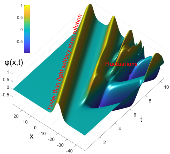
Figure 1: Numerical simulation of the motion of an FTL solitary wave solution (9) of a real nonlinear KG system (1). The potential (7) in the range $0<\varphi<1$ is negative, then the system and its solutions are essentially unstable. Hence, the emergence of some spontaneous fluctuations is related to this inherent instability of the system (1).

Numerically or theoretically, it is easy to show that the new FTL solitary wave solution (9) is essentially unstable. For example, based on a finite difference method for the PDE (3), one can simply simulate the motion of the special solitary solution (9) in Matlab for $v=2$. For a brief but remarkable time, it can be seen that a localized solitary wave solution at an FTL speed can actually exist in our simulation program (see Fig. 1). After a while, the form of the FTL solitary wave solution (9) does not remain stationary and gets disrupted along the time.

In general, according to the Noether’s theorem, the energy density and momentum density, which belong to the Lagrangian density (1) would be

$$\varepsilon(x,t)=\dot{\varphi}^{2}+\varphi^{\prime 2}+U(\varphi),\quad\textrm{and}\quad p(x,t)=-2\dot{\varphi}\varphi^{\prime},$$ (10)

respectively. The integration of these functions over the whole space, for any arbitrary localized solution, yields the related total energy and total momentum. Therefore, if one applies these integrations for the FTL solitary wave solution (9), the following results are obtained:

$$E_{v}=\int_{-\infty}^{\infty}[\dot{\varphi_{v}}^{2}+\varphi_{v}^{\prime 2}+U(\varphi_{v})]dx=\sqrt{\frac{2\pi}{v^{2}-1}},$$ (11)

and

$$P=\int_{-\infty}^{\infty}[-2\dot{\varphi_{v}}\varphi_{v}^{\prime}]dx=v\sqrt{\frac{2\pi}{v^{2}-1}}.$$ (12)

Contrary to what we expect, higher speeds here do not lead to larger total energies. In fact, a moving solitary wave solution at the speed of light has infinite energy, while the one moving at $v\rightarrow\infty$ has $E_{v}\rightarrow 0$. In regard to Fig. 1, numerical calculations show that despite the instability of the system and the occurrence of some fluctuations, total energy and total momentum remain constat according to Eqs. (11) and (12) for case $v=2$, meaning that the energy and momentum conservation laws are valid for such a system as we expected. Moreover, if one expects the same standard relativistic relations $E=\gamma E_{o}$, and $P=\gamma E_{o}$ to remain valid for the FTL solitary wave solution (9), the rest energy must be an imaginary value $E_{o}=i\sqrt{2\pi}$, resulting from an imaginary mass.

3 A zero-energy soliton solution at FTL speeds

In general, for a set of relativistic scalar fields $\phi_{i}$ ($i=1,\cdots,N$), the standard Lagrangian densities are functions of the fields and the kinetic scalars ${\cal S}_{ij}=\partial_{\mu}\phi_{i}\partial^{\mu}\phi_{j}$:

$${\cal L}={\cal L}(\phi_{r},{\cal S}_{ij}),$$ (13)

where $i,j,r=1,\cdots,N$. According to the principle of least action, the dynamical equations of motion would be:

$$\frac{\partial{\cal L}}{\partial\phi_{i}}-\frac{\partial}{\partial x^{\mu}}\left(\frac{\partial{\cal L}}{\partial\phi_{i,\mu}}\right)=\frac{\partial{\cal L}}{\partial\phi_{i}}-\sum_{j=1}^{N}(1+\delta_{ij})\left[\frac{\partial}{\partial x^{\mu}}\left(\frac{\partial{\cal L}}{\partial{\cal S}_{ij}}\right)\partial^{\mu}\phi_{j}+\frac{\partial{\cal L}}{\partial{\cal S}_{ij}}\partial_{\mu}\partial^{\mu}\phi_{j}\right]=0.$$ (14)

Since the Lagrangian density (13) is invariant under the infinitesimal space-time translations, there are four continuity equations $\partial_{\mu}T^{\mu\nu}=0$ and four conserved quantities $P^{\mu}=\int T^{o\mu}d^{3}\textbf{x}$, where

$$T^{\mu\nu}=\sum_{i=1}^{N}\frac{\partial{\cal L}}{\partial\phi_{i,\mu}}\frac{\partial\phi_{i}}{\partial x_{\nu}}-{\cal L}g^{\mu\nu}$$ (15)

is called the energy-momentum tensor and $g^{\mu\nu}$ is the Minkowski metric. The $T^{00}$ component of the energy-momentum tensor is the same as energy density function:

$$T^{00}=\varepsilon=\sum_{i=1}^{N}\frac{\partial{\cal L}}{\partial\dot{\phi}_{i}}\dot{\phi}_{i}-{\cal L}=\sum_{j=1}^{N}\sum_{i=1}^{N}\frac{\partial{\cal L}}{\partial{\cal S}_{ij}}\dot{\phi}_{i}\dot{\phi}_{j}(\delta_{ij}+1)-{\cal L}.$$ (16)

A zero-energy solitary wave solution can be introduced as a special localized solution for which the energy density function (16) is zero everywhere. More precisely, a zero-energy solution is a special solution of $N$ coupled PDEs (14) for which $\varepsilon=0$. Condition $\varepsilon=0$ can be interpreted as a new PDE along with $N$ coupled PDEs (14). It is mathematically unlikely that $N+1$ coupled PDEs have a common solution for $N$ fields. However, if the Lagrangian density is such that it and all its derivatives, i.e. ${\cal L}$, $\frac{\partial{\cal L}}{\partial\phi_{i}}$, $\frac{\partial{\cal L}}{\partial{\cal S}_{ij}}$, and $\frac{\partial}{\partial x^{\mu}}(\frac{\partial{\cal L}}{\partial{\cal S}_{ij}})$, become zero simultaneously for a special solution, thus those $N+1$ PDEs will be satisfied automatically and the special solution would be a zero-energy solution. Such a situation is possible only if the Lagrangian density would be a function of the powers of some scalar functionals, which are all zero simultaneously for a special solution. More precisely, for several scalar fields $\phi_{i}$ ($i=1,\cdots,N$), if there are a number of independent scalars $\mathbb{S}_{j}$ ($j=1,\cdots,m$), which are all zero simultaneously ($\mathbb{S}_{j}=0$) for a special solution, the general form of an extended KG Lagrangian density ($k$-field) with a zero-energy solution is:

$${\cal L}=\sum_{n_{1}=0}^{\infty}\sum_{n_{2}=0}^{\infty}\cdots\sum_{n_{m}=0}^{\infty}a({n_{1},\cdots,n_{m}})\mathbb{S}_{1}^{n_{1}}\mathbb{S}_{2}^{n_{2}}\cdots\mathbb{S}_{m}^{n_{m}},$$ (17)

provided $n_{1}+n_{2}+\cdots+n_{m}\geqslant 3$. Note that, scalars $\mathbb{S}_{j}$ ($j=1,\cdots,m$) and coefficients $a({n_{1},\cdots,n_{m}})$ can be arbitrary well-defined functions of the fields and the kinetic scalars ${\cal S}_{ij}$. For example, for a single scalar field $\phi$, an arbitrary scalar functional $\mathbb{S}={\cal S}+4\varphi^{2}\ln|\varphi|$ (${\cal S}=\partial_{\mu}\varphi\partial^{\mu}\varphi$) can be introduced, that $\varphi=\pm\exp(x^{2})$ is a solution for condition $\mathbb{S}=0$. Hence, this solution would be a canonical zero-energy solution for Lagrangian density ${\cal L}=\mathbb{S}^{3}$ as well. In fact, for ${\cal L}=\mathbb{S}^{3}$ we have $\frac{\partial{\cal L}}{\partial\phi}=3\mathbb{S}^{2}\frac{\partial\mathbb{S}}{\partial\phi}$, $\frac{\partial{\cal L}}{\partial{\cal S}}=3\mathbb{S}^{2}$, and $\frac{\partial}{\partial x^{\mu}}(\frac{\partial{\cal L}}{\partial{\cal S}})=6\mathbb{S}\frac{\partial\mathbb{S}}{\partial x^{\mu}}$, which obviously are all zero for condition $\mathbb{S}=0$.

Based on what we have said so far, finding a relativistic system of fields with a zero-energy solution does not seem difficult. However, if we want to have such a solution that fully satisfies the energetical stability considerations, there is not an easy task ahead of us. A solitary wave solution is energetically stable if any arbitrary variation above its background leads to an increase in the total energy. Therefore, the energetical stability condition imposes serious restrictions on the series (17), which causes it to be turned to special formats. In this regard, we introduce an extended KG system with a single energetically stable FTL solitary wave solution in $1+1$ dimensions. For this purpose, three scalar fields $\varphi$, $\theta$ and $\psi$ are used to introduce a proper Lagrangian density. First, we introduce five independent relativistic functional scalars as follows:

$$\mathbb{S}_{1}=\partial_{\mu}\theta\partial^{\mu}\theta-1,$$ (18)

$$\mathbb{S}_{2}=\partial_{\mu}\varphi\partial^{\mu}\varphi+4\varphi^{2}\ln|\varphi|,$$ (19)

$$\mathbb{S}_{3}=\partial_{\mu}\varphi\partial^{\mu}\varphi+4\varphi\psi,$$ (20)

$$\mathbb{S}_{4}=\partial_{\mu}\psi\partial^{\mu}\psi+4\psi^{2}\ln|\varphi|+8\psi^{2}+4\psi\varphi,$$ (21)

$$\mathbb{S}_{5}=\partial_{\mu}\psi\partial^{\mu}\psi+4\varphi^{2}\ln|\varphi|(\ln|\varphi|+1)^{2}.$$ (22)

Apart from $\mathbb{S}_{1}$, these scalars are built deliberately in such a way that four conditions $\mathbb{S}_{i}=0$ ($i=2,3,4,5$), as four independent PDEs, have a unique common solution at rest in the following form:

$$\varphi_{o}=\pm\exp(x^{2}),\quad\psi_{o}=\pm x^{2}\exp(x^{2}).$$ (23)

The moving version of this solution would be:

$$\varphi_{v}=\pm\exp(\gamma^{2}(x-vt)^{2}),\quad\psi_{v}=\pm\gamma^{2}(x-vt)^{2}\exp(\gamma^{2}(x-vt)^{2}).$$ (24)

Although such functions for speeds less than the speed of light are non-localized, but for the FTL speeds $v>1$, they turn to localized functions:

$$\varphi_{v}=\pm\exp\left(\frac{-(x-vt)^{2}}{v^{2}-1}\right),\quad\psi_{v}=\frac{\mp(x-vt)^{2}}{v^{2}-1}\exp\left(\frac{-(x-vt)^{2}}{v^{2}-1}\right),$$ (25)

which together can be considered as a localized FTL solution for four independent conditions $\mathbb{S}_{i}=0$ ($i=2,3,4,5$).

Now, we build the Lagrangian density,

$${\cal L}=B\sum_{i=1}^{5}{\cal K}_{i}^{3},$$ (26)

where $B$ is a positive constant, and

$${\cal K}_{1}=h_{1}^{2}\mathbb{S}_{1},$$ (27)

$${\cal K}_{2}=h_{2}^{2}\mathbb{S}_{1}+\mathbb{S}_{2},$$ (28)

$${\cal K}_{3}=h_{3}^{2}\mathbb{S}_{1}+\mathbb{S}_{3},$$ (29)

$${\cal K}_{4}=h_{4}^{2}\mathbb{S}_{1}+\mathbb{S}_{4},$$ (30)

$${\cal K}_{5}=h_{5}^{2}\mathbb{S}_{1}+\mathbb{S}_{5},$$ (31)

$$h_{1}=\varphi,$$ (32)

$$h_{2}=\varphi(2\ln|\varphi|+1)$$ (33)

$$h_{3}=2\varphi+\psi$$ (34)

$$h_{4}=2\varphi+5\psi+2\psi\ln|\varphi|$$ (35)

$$h_{5}=\sqrt{2}\varphi(\ln|\varphi|+1)^{2}.$$ (36)

Note that, since ${\cal K}_{i}$ ($i=1,2,\cdots,5$) are introduced as five independent linear combinations of $\mathbb{S}_{i}$ ($i=1,2,\cdots,5$), five conditions $\mathbb{S}_{i}=0$ are equivalent to ${\cal K}_{i}=0$ ($i=1,2,\cdots,5$).

Using the Euler-Lagrange equations (14) for the new Lagrangian density (26), one can easily obtain the related dynamical equations:

$$\sum_{i=1}^{5}{\cal K}_{i}\left[2(\partial_{\mu}{\cal K}_{i})\frac{\partial{\cal K}_{i}}{\partial(\partial_{\mu}\theta)}+{\cal K}_{i}\partial_{\mu}\left(\frac{\partial{\cal K}_{i}}{\partial(\partial_{\mu}\theta)}\right)\right]=0,$$ (37)

$$\sum_{i=1}^{5}{\cal K}_{i}\left[2(\partial_{\mu}{\cal K}_{i})\frac{\partial{\cal K}_{i}}{\partial(\partial_{\mu}\varphi)}+{\cal K}_{i}\partial_{\mu}\left(\frac{\partial{\cal K}_{i}}{\partial(\partial_{\mu}\varphi)}\right)-{\cal K}_{i}\frac{\partial{\cal K}_{i}}{\partial\varphi}\right]=0,$$ (38)

$$\sum_{i=1}^{5}{\cal K}_{i}\left[2(\partial_{\mu}{\cal K}_{i})\frac{\partial{\cal K}_{i}}{\partial(\partial_{\mu}\psi)}+{\cal K}_{i}\partial_{\mu}\left(\frac{\partial{\cal K}_{i}}{\partial(\partial_{\mu}\psi)}\right)-{\cal K}_{i}\frac{\partial{\cal K}_{i}}{\partial\psi}\right]=0.$$ (39)

Moreover, the related energy density function would be

$$\varepsilon(x,t)=\frac{\partial{\cal L}}{\partial\dot{\theta}}\dot{\theta}+\frac{\partial{\cal L}}{\partial\dot{\varphi}}\dot{\varphi}+\frac{\partial{\cal L}}{\partial\dot{\psi}}\dot{\psi}-{\cal L}=\sum_{i=1}^{5}B{\cal K}_{i}^{2}\left[3C_{i}-{\cal K}_{i}\right]=\sum_{i=1}^{5}\varepsilon_{i},$$ (40)

which is divided into five distinct parts, in which

$$C_{i}=\dfrac{\partial{\cal K}_{i}}{\partial\dot{\theta}}\dot{\theta}+\dfrac{\partial{\cal K}_{i}}{\partial\dot{\varphi}}\dot{\varphi}+\dfrac{\partial{\cal K}_{i}}{\partial\dot{\psi}}\dot{\psi}=\begin{cases}2h_{1}^{2}\dot{\theta}^{2}&\text{i=1}\\ 2h_{2}^{2}\dot{\theta}^{2}+2\dot{\varphi}^{2}&\text{i=2}\\ 2h_{3}^{2}\dot{\theta}^{2}+2\dot{\varphi}^{2}&\text{i=3}.\\ 2h_{4}^{2}\dot{\theta}^{2}+2\dot{\psi}^{2}&\text{i=4}.\\ 2h_{5}^{2}\dot{\theta}^{2}+2\dot{\psi}^{2}&\text{i=5}.\end{cases}$$ (41)

After a straightforward calculation, one can obtain:

$$\varepsilon_{1}=B{\cal K}_{1}^{2}[5h_{1}^{2}\dot{\theta}^{2}+h_{1}^{2}\theta^{\prime 2}+\varphi^{2}]\geq 0,$$ (42)

$$\varepsilon_{2}=B{\cal K}_{2}^{2}[5h_{2}^{2}\dot{\theta}^{2}+h_{2}^{2}\theta^{\prime 2}+5\dot{\varphi}^{2}+\varphi^{\prime 2}+\varphi^{2}+4(\varphi\ln|\varphi|)^{2}]\geq 0,$$ (43)

$$\varepsilon_{3}=B{\cal K}_{3}^{2}[5h_{3}^{2}\dot{\theta}^{2}+h_{3}^{2}\theta^{\prime 2}+5\dot{\varphi}^{2}+\varphi^{\prime 2}+4\varphi^{2}+4\psi^{2}]\geq 0,$$ (44)

$$\varepsilon_{4}=B{\cal K}_{4}^{2}[5h_{4}^{2}\dot{\theta}^{2}+h_{4}^{2}\theta^{\prime 2}+5\dot{\psi}^{2}+\psi^{\prime 2}+2\psi^{2}+4(\varphi+2\psi+\psi\ln|\varphi|)^{2}]\geq 0,$$ (45)

$$\varepsilon_{5}=B{\cal K}_{5}^{2}[5h_{5}^{2}\dot{\theta}^{2}+h_{5}^{2}\theta^{\prime 2}+5\dot{\psi}^{2}+\psi^{\prime 2}+2\varphi^{2}(1+\ln^{2}|\varphi|)(1+\ln|\varphi|)^{2}]\geq 0.$$ (46)

Since all bracket terms $[\cdots]$ in Eqs. (37)-(40) and (42)-(46) are multiplied by the scalar functionals ${\cal K}_{i}$ or ${\cal K}_{i}^{2}$ ($i=1,2,\cdots,5$), any set of functions $\theta$, $\varphi$ and $\psi$ for which ${\cal K}_{i}=0$ ($\mathbb{S}_{i}=0$) simultaneously, is a special zero-energy solution. As mentioned before, for four conditions $\mathbb{S}_{i}=0$ ($i=2,3,4,5$), there is a unique localized common solution (25). However, the condition $\mathbb{S}_{1}=0$, which is in no way related to other conditions $\mathbb{S}_{i}=0$ ($i=2,3,4,5$), has diverging solutions such as $\theta_{v}=\pm t$, $\theta_{v}=\frac{1}{\sqrt{3}}(2t-x)$, $\theta_{v}=\frac{1}{\sqrt{12}}(4t+2x)$, and so on. Hence, for a zero-energy localized solution, for which ${\cal K}_{i}=0$ ($i=1,2,\cdots,5$), the form of $\varphi$ and $\psi$ are unique (25), but $\theta$ can be considered as a free field, provided it satisfies the constraint $\partial_{\mu}\theta\partial^{\mu}\theta=1$. In fact, the field $\theta$ is expected to introduce a system for which all the terms in the energy density function will be positive definite.

In general, according to Eqs. (42)-(46), all the terms in the energy density function are positive definite and all ${\cal K}_{i}$’s ($i=1,2,3,4,5$), and subsequently all $\varepsilon_{i}$’s, are zero simultaneously just for the special solution (25). Therefore, for any arbitrary variation above the background of the special solution (25), at least one of the ${\cal K}_{i}$’s ($i=1,2,3,4,5$) would be a non-zero function, and then the energy density function changes to a non-zero positive function. Thus, for any arbitrary variation, the total energy always increases. In other words, the special solution (25) has the minimum total energy among the other solutions, meaning that it is energetically stable and then it is a soliton solution. More precisely, for any arbitrary (non-trivial) small variations $\delta\varphi$, $\delta\psi$, and $\delta\theta$ above the background of the special solution (25), i.e. $\varphi=\varphi_{v}+\delta\varphi$, $\psi=\psi_{v}+\delta\psi$, and $\theta=\theta_{v}+\delta\theta$, if one investigates $\varepsilon_{i}$ ($i=1,2,3,4,5$), and keep the terms to the least order of variations, it yields

$$\delta\varepsilon_{i}=B[3(C_{i}+\delta C_{i})({\cal K}_{i}+\delta{\cal K}_{i})^{2}-({\cal K}_{i}+\delta{\cal K}_{i})^{3}]=B[3(C_{i}+\delta C_{i})(\delta{\cal K}_{i})^{2}-(\delta{\cal K}_{i})^{3}]\approx$$

$$\quad\quad B[3C_{i}(\delta{\cal K}_{i})^{2}-(\delta{\cal K}_{i})^{3}]\approx B[3C_{i}(\delta{\cal K}_{i})^{2}]>0,\quad\quad$$ (47)

where ${\cal K}_{i}=0$ and $\varepsilon_{i}=0$ ($i=1,2,3,4,5$) for the special solution (25). Therefore, according to Eq. (3), since $C_{i}>0$, $\delta\varepsilon_{i}$ ($i=1,2,\cdots,5$), and then $\delta E$, are always positive definite for all small variations, that is, the special solution (25) is energetically stable. It should be noted again that, since ${\cal K}_{i}$’s ($i=1,2,\cdots,5$) are five completely independent functionals of three scalar fields $\theta$, $\varphi$ and $\psi$, it is not possible for them to be zero simultaneously except when the special solution (25) along with one of the solutions of $\mathbb{S}_{1}=0$. For extra evidence, let us consider the energy variations for a number of arbitrary small deformations above the background of the special solution (25) numerically. For example, twelve arbitrary (ad hoc) deformations can be introduced as follows:

$$\varphi=\pm\exp\left(\frac{-(1+\xi)\tilde{x}^{2}}{v^{2}-1}\right),\quad\psi=\frac{\mp\tilde{x}^{2}}{v^{2}-1}\exp\left(\frac{-\tilde{x}^{2}}{v^{2}-1}\right),\quad\quad\quad$$ (48)

$$\varphi=\pm\exp\left(\frac{-(1+\xi)\tilde{x}^{2}}{v^{2}-1}\right),\quad\psi=\frac{\mp\tilde{x}^{2}}{v^{2}-1}\exp\left(\frac{-(1+\xi)\tilde{x}^{2}}{v^{2}-1}\right),$$ (49)

$$\varphi=\pm(1+\xi)\exp\left(\frac{-\tilde{x}^{2}}{v^{2}-1}\right),\quad\psi=\frac{\mp(1+\xi)\tilde{x}^{2}}{v^{2}-1}\exp\left(\frac{-\tilde{x}^{2}}{v^{2}-1}\right),$$ (50)

$$\varphi=\pm(1+\xi)\exp\left(\frac{-\tilde{x}^{2}}{v^{2}-1}\right),\quad\psi=\frac{\mp\tilde{x}^{2}}{v^{2}-1}\exp\left(\frac{-\tilde{x}^{2}}{v^{2}-1}\right),$$ (51)

$$\varphi=\pm\exp\left(\frac{-\tilde{x}^{2}}{v^{2}-1+\xi}\right),\quad\psi=\frac{\mp\tilde{x}^{2}}{v^{2}-1+\xi}\exp\left(\frac{-\tilde{x}^{2}}{v^{2}-1+\xi}\right),$$ (52)

$$\varphi=\pm\exp\left(\frac{-\tilde{x}^{2}}{v^{2}-1}\right),\quad\psi=\frac{\mp(1+\xi)\tilde{x}^{2}}{v^{2}-1}\exp\left(\frac{-\tilde{x}^{2}}{v^{2}-1}\right),$$ (53)

$$\varphi=\pm\exp\left(\frac{-\tilde{x}^{2}}{v^{2}-1}\right)+\xi\tilde{x}\exp(-\tilde{x}^{2}),\quad\psi=\frac{\mp\tilde{x}^{2}}{v^{2}-1}\exp\left(\frac{-\tilde{x}^{2}}{v^{2}-1}\right),$$ (54)

$$\varphi=\pm\exp\left(\frac{-(x-(1+\xi)vt)^{2}}{v^{2}-1}\right),\quad\psi=\frac{\mp\tilde{x}^{2}}{v^{2}-1}\exp\left(\frac{-(x-(1+\xi)vt)^{2}}{v^{2}-1}\right),\quad\quad$$ (55)

$$\varphi=\pm\exp\left(\frac{-\tilde{x}^{2}}{v^{2}-1}\right),\quad\psi=\frac{\mp\tilde{x}^{2}}{v^{2}-1}\exp\left(\frac{-\tilde{x}^{2}}{v^{2}-1}\right),\quad\theta=(1+\xi)t$$ (56)

$$\varphi=\pm\exp\left(\frac{-\tilde{x}^{2}}{v^{2}-1}\right),\quad\psi=\frac{\mp(x-vt+\xi)^{2}}{v^{2}-1}\exp\left(\frac{-\tilde{x}^{2}}{v^{2}-1}\right),$$ (57)

$$\varphi=\pm\exp\left(\frac{-\tilde{x}^{2}}{v^{2}-1}\right)+\xi\exp(-x^{2}),\quad\psi=\frac{\mp\tilde{x}^{2}}{v^{2}-1}\exp\left(\frac{-\tilde{x}^{2}}{v^{2}-1}\right),$$ (58)

$$\varphi=\pm\exp\left(\frac{-\tilde{x}^{2}}{v^{2}-1}\right),\quad\psi=\frac{\mp\tilde{x}^{2}}{v^{2}-1}\exp\left(\frac{-\tilde{x}^{2}}{v^{2}-1}\right)+\xi t\exp(-\tilde{x}^{2}).$$ (59)

where $\tilde{x}=x-vt$, and $\xi$ is a small parameter, which can be considered as an indication of the order of small deformations. The case $\xi=0$ leads to the same special solution (25). For such arbitrary deformations (48)-(58) at $t=0$ and $v=2$, Fig. 2 demonstrates that a larger deformation leads to a further increase in the total energy, as we expected. Except for Eq. (56), the catalyzer field $\theta$ is considered to be one of the solutions of $\mathbb{S}_{1}=0$ for all arbitrary deformations. Furthermore, it is obvious that parameter $B$ has a main role in the stability of the special solution (25), and its larger values lead to more stability of the special solution (25). To put it differently, the larger the values, the greater will be the increase in the total energy for any arbitrary small variation above the background of the special solution (25).

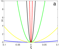
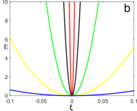
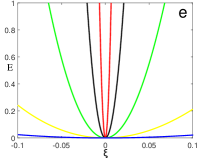
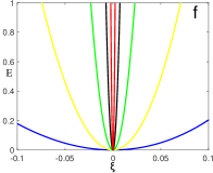
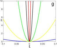
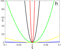
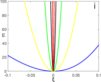
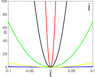
Figure 2: Plots. a-l represent variations of the total energy $E$ versus small $\xi$ for different deformations (48)-(59) at $t=0$ and $v=2$ in the context of system (26). Various colored curves blue, yellow, green, black, and red are related to $B=1$, $B=10$, $B=100$, $B=1000$, and $B=10000$, respectively.

For the vacuum solution, i.e. $\varphi=\psi=0$, according to Eqs. (42)-(46), since $h_{i}$’s$=0$ ($i=1,2,\cdots,5$), all $\varepsilon_{i}$’s$=0$ ($i=1,2,\cdots,5$). This means, when $\varphi=\psi=0$, it is not at all important what the form of the scalar field $\theta$ is. However, when $\varphi\neq 0$ and $\psi\neq 0$, to have a zero-energy solitary wave solution (25), $\theta$ must satisfy the equation $\partial_{\mu}\theta\partial^{\mu}\theta=1$ (i.e. $\mathbb{S}_{1}=0$). In summary, the role of the phase field $\theta$ is like a path in all space, along which the zero-energy particle (25) is stable and moves freely.

4 A nonzero-energy soliton solution at FTL speeds

We can now combine the models introduced in sections 2 and 3 and introduce a new model as follows:

$${\cal L}={\cal L}_{o}+{\cal L}_{cat}=\left[\partial^{\mu}\varphi\partial_{\mu}\varphi-U(\varphi)\right]+[B\sum_{i=1}^{5}{\cal K}_{i}^{3}],$$ (60)

where ${\cal L}_{o}$ and ${\cal L}_{cat}$ are the same Lagrangian densities which are introduced in Eqs. (1) and (26), respectively. In this model, $U(\varphi)=4\varphi^{2}\ln(|\varphi|)$, and ${\cal L}_{cat}$ can be called the catalyzer Lagrangian density. For the new system (60), the general dynamical equations would be:

$$\sum_{i=1}^{5}{\cal K}_{i}\left[2(\partial_{\mu}{\cal K}_{i})\frac{\partial{\cal K}_{i}}{\partial(\partial_{\mu}\theta)}+{\cal K}_{i}\partial_{\mu}\left(\frac{\partial{\cal K}_{i}}{\partial(\partial_{\mu}\theta)}\right)\right]=0,$$ (61)

$$\left[\Box\varphi+\frac{1}{2}\frac{dU}{d\varphi}\right]+\frac{3}{2}B\sum_{i=1}^{5}{\cal K}_{i}\left[2(\partial_{\mu}{\cal K}_{i})\frac{\partial{\cal K}_{i}}{\partial(\partial_{\mu}\varphi)}+{\cal K}_{i}\partial_{\mu}\left(\frac{\partial{\cal K}_{i}}{\partial(\partial_{\mu}\varphi)}\right)-{\cal K}_{i}\frac{\partial{\cal K}_{i}}{\partial\varphi}\right]=0,\quad\quad$$ (62)

$$\sum_{i=1}^{5}{\cal K}_{i}\left[2(\partial_{\mu}{\cal K}_{i})\frac{\partial{\cal K}_{i}}{\partial(\partial_{\mu}\psi)}+{\cal K}_{i}\partial_{\mu}\left(\frac{\partial{\cal K}_{i}}{\partial(\partial_{\mu}\psi)}\right)-{\cal K}_{i}\frac{\partial{\cal K}_{i}}{\partial\psi}\right]=0.$$ (63)

Moreover, the corresponding energy density function of the new system (60) would be:

$$\varepsilon(x,t)=\varepsilon_{o}+\varepsilon_{cat}=[\dot{\varphi}^{2}+\varphi^{\prime 2}+U(\varphi)]+\sum_{i=1}^{5}B{\cal K}_{i}^{2}\left[3C_{i}-{\cal K}_{i}\right].$$ (64)

where $\varepsilon_{o}$ and $\varepsilon_{cat}$ belonging to Lagrangian densities ${\cal L}_{o}$ and ${\cal L}_{cat}$, respectively.

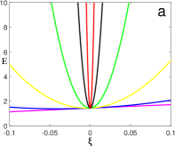
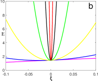
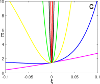
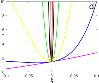
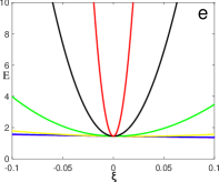
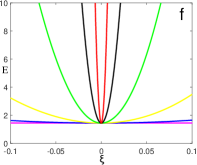
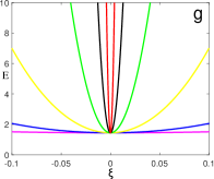
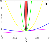
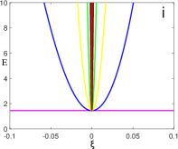
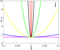
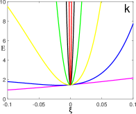
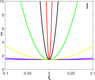
Figure 3: Plots. a-l are representing variations of the total energy $E$ versus small $\xi$ for different deformations (48)-(59) at $t=0$ and $v=2$ in the context of the new system (60). Various color curves of purple, blue, yellow, green, black, and red are related to $B=0$, $B=1$, $B=10$, $B=100$, $B=1000$, and $B=10000$, respectively. These Figs. confirm how larger values of parameter $B$ lead to more stability. In other words, the larger the value of $B$, the greater will be the increase in the total energy for any arbitrary small variation above the background of the FTL soliton solution (25).

For the coupled dynamical equations (61)-(63), the same Eq. (25) would again be a solution, but now it is not a zero-energy FTL solution anymore. In fact, for $\varphi_{v}=\pm\exp\left(-\tilde{x}^{2}/(v^{2}-1)\right)$, the expression $\Box\varphi+\frac{1}{2}\frac{dU}{d\varphi}$ would be independently zero. Furthermore, ${\cal K}_{i}$’s are all independently zero for the special solution (25) provided $\theta$ is one of the solutions of $\mathbb{S}_{1}=0$. Hence, all dynamical equations (61)-(63) are satisfied automatically for the special solution (25) along with one of the solutions of $\mathbb{S}_{1}=0$. More precisely, just for the special solution (25), all terms in the dynamical equations, that contain ${\cal K}_{i}$ and ${\cal K}_{i}^{2}$, would be automatically zero, and then the dynamical equations (61)-(63) are reduced to $\Box\varphi+\frac{1}{2}\frac{dU}{d\varphi}=0$ as the dominant dynamical equation of the special solution (25). Since $\varepsilon_{cat}$ is zero for the special solution (25), the total energy and momentum as a function of the speed is the same which was obtained in Eqs. (11) and (12), respectively. In other words, only the first part of the Lagrangian density (60) is responsible to generate energy and momentum for the special solution (25).

In general, it can be proved that the special solution (25) is again an energetically stable entity provided we use a system with a large parameter $B$. For any arbitrary small deformation $\delta\varphi$, $\delta\psi$, and $\delta\theta$ above the background of the special solution (25), which is not now a zero energy FTL soliton in the new model (60), the variation of the energy density function would be:

$$\delta\varepsilon=\delta\varepsilon_{o}+\delta\varepsilon_{cat}\approx\left(2\dot{\varphi}_{v}\delta\dot{\varphi}+2\varphi^{\prime}_{v}\delta\varphi^{\prime}+\frac{dU}{d\varphi}\delta\varphi\right)+\sum_{i=1}^{5}[3BC_{i}(\delta{\cal K}_{i})^{2}].\quad\quad$$ (65)

The second term in the energy density variation, i.e. $\delta\varepsilon_{cat}$, is a positive definite functional of the second order of variations. However, the first term, i.e. $\delta\varepsilon_{o}$, is a functional of the first order of variation $\delta\varphi$ and is not positive definite. Normally, we expect to exclude the terms that contain second-order of variations as opposed to the terms that contain first-order of variations. It should be noted that $\delta\varepsilon_{cat}$ contains parameter $B$, but $\delta\varepsilon_{o}$ does not, thus, the comparison between them needs to be examined more closely. For example, for the case $B=10^{40}$, the inequality $|\delta\varphi|>B(\delta\varphi)^{2}$ is fulfilled only for the very small variations less than $10^{-20}$, which are not physically significant. It means that the larger the value of $B$, the smaller variations required for validation of the inequality $|\delta\varphi|>B(\delta\varphi)^{2}$. Likewise, a similar comparison can be used between $|\delta\varepsilon_{o}|$ and $\delta\varepsilon_{cat}$. In other words, $|\delta\varepsilon_{o}|$ would be larger than $\delta\varepsilon_{cat}$ only for the very small variations; meaning that, only for such physically unimportant very small variations, $\delta\varepsilon=\delta\varepsilon_{o}+\delta\varepsilon_{cat}$ may not be a positive function, and then $\delta E=\int\delta\varepsilon d^{3}x$ may have a very small negative value (see Fig. 3). Accordingly, for such very small variations $\delta\varphi$, the special solution (25) may not be an energetically stable entity. However, they are so small physically that can be ignored in terms of energetical stability criterion. To summarize, for a large enough value of $B$, $\delta\varepsilon$ is always positive for all significant physical variations and then the stability of the special solution (25) would guaranteed appreciably in the context of the new system (60). Hence, just for some unimportant too small variations, it may be possible to see the violation of the energetical stability criterion, but the energy reduction for these variations are so small that they can be ignored physically.

Furthermore, it can be possible to show that the special solution (25) is really an energetically stable entity numerically. For example , we can study numerically the variation of the total energy for all arbitrary deformations (48)-(59) in the context of the new system (60) again. Figure 3, which is obtained for $v=2$, demonstrates that for large values of parameter $B$, the energetical stability of the special solution (25) would be guaranteed. Similar figures can be obtained for other FTL velocities. In fact, the catalyzer Lagrangian density ${\cal L}_{cat}$ behaves like a massless spook, which surrounds the special solution (25) and opposes any internal deformation. Although, the catalyzer term strongly guarantees the stability of the special solution (25), but it does not appear in any of the observable, and that is why we call it the stability catalyzer. In sum, the new model (60) with a large value of parameter $B$, leads to a nonzero-energy energetically stable solitary wave solution (25), which moves at FTL speeds. Moreover, Fig. 3 shows that clearly why the case $B=0$ leads to an unstable solitary wave solution. In other words, the case $B=0$ is the same original nonlinear KG system (1) for which the energy of the solitary wave solution (9) is not a minimum against any arbitrary deformation.

Since the special solution (25) is non-topological, a multi particle-like version of that can be easily constructed. In general, the non-topological solutions are zero at far distances, hence when they are too far apart, the tail of each non-topological solution would be zero at the position of the others. In other words, the effect of each non-topological solution on the other solutions is practically zero when the relative distances between them are large enough. Therefore, adding any arbitrary number of the special solutions (25) together, when they are initially far enough apart, would still be approximately a solution. In fact, the greater the distances between the non-topological solutions, the more accurate this approximation will be. For example, adding four distinct special solutions (25), which initially have different velocities $v_{i}$ ($i=1,2,3,4$) and stand at different positions $x_{i}$ is again a solution at the initial times (the times that are close to $t=0$):

$$\varphi=\sum_{i=1}^{4}\left[\pm\exp\left(\frac{-(x-v_{i}t-x_{i})^{2}}{v_{i}^{2}-1}\right)\right],$$

$$\psi=\sum_{i=1}^{4}\left[\frac{\mp(x-v_{i}t-x_{i})^{2}}{v_{i}^{2}-1}\exp\left(\frac{-(x-v_{i}t-x_{i})^{2}}{v_{i}^{2}-1}\right)\right],$$ (66)

provided that $|x_{i+1}-x_{i}|$ be large enough. For such a linear combination (4), it was observed numerically that the terms $\mathbb{S}_{i}$ ($i=1,\cdots,5$) are all approximately zero. Hence, based on dynamical equations (61)-(63), such a linear combination (4) would be approximately a solution again. The energy density function of this combination equals the sum of four distinct lumps moving towards each other, as we expected (see Fig. 4).

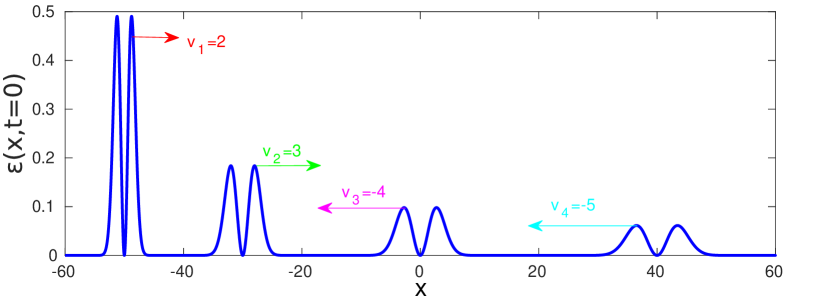
Figure 4: The energy density representation of a four-particle-like solution (4) at $t=0$ in the context of the new system (60) with $B=10^{10}$. We set the initial velocities and the initial positions to $v_{1}=2$, $v_{2}=3$, $v_{3}=-4$, $v_{4}=-5$, $x_{1}=-50$, $x_{2}=-30$, $x_{3}=0$, and $x_{4}=40$, respectively.

For a multi particle-like solution, the phase field $\theta$ can change from one solution to another. In regions between two special solutions, the scalar fields $\varphi$, $\psi$ are zero everywhere. Thus, there is not any rigorous restriction on $\theta$ to be one of the solutions of the condition $\mathbb{S}_{1}=0$. In other words, where the scalar fields $\varphi$, $\psi$ are almost zero, the phase field $\theta$ is completely free and evolves without any rigorous restriction. For example, if there is a two-particle-like solution, the phase field can change from $\theta_{1}=\pm t$ at the position of the first special solution to $\theta_{2}=\frac{1}{\sqrt{3}}(2t-x)$ at the position of the second one; or it may not change at all and have a definite form, e.g. $\theta=\pm t$, throughout the space, independent of any number of particle-like solutions.

5 Summary and Conclusion

For the relativistic classical field systems in $1+1$ dimensions, there is a general rule to obtain the form of a moving solution from its known non-moving version, by using $x\rightarrow\gamma(x-vt)$ and $t\rightarrow\gamma(t-vx)$ according to the Lorentz transformations, where $\gamma=1/\sqrt{1-v^{2}}$. Based on this general rule, if one finds a localized solution at rest, it turns to a localized solitary wave solution moving at arbitrary speed ($v<1$). However, for a non-localized solution at rest, which is a function of $x^{2}$, $t^{2}$, and $xt$, it may turn to a localized solitary wave solution at FTL speeds. In fact, with speeds faster than the speed of light, $\gamma$ would be a pure imaginary number, but the even powers of $\gamma$ would be a real number. Thus, for FTL speeds: $x^{2}\rightarrow\frac{-1}{v^{2}-1}(x-vt)^{2}$, $t^{2}\rightarrow\frac{-1}{v^{2}-1}(t-vx)^{2}$, and $xt\rightarrow\frac{-1}{v^{2}-1}(x-vt)(t-vx)$ which remain real expressions. For example, a relativistic field system with a special non-localized solution $\varphi=\exp(x^{2})$ at rest, is not physically interesting since it is not square integrable, but for $v>1$ it turns to a localized real function $\varphi=\exp(\frac{-1}{v^{2}-1}(x-vt)^{2})$, which can be physically interesting. Therefore, obtaining a special non-moving solution of a nonlinear field system may not be of physical importance, but it may turn to an interesting localized moving solution at FTL speeds.

In this paper, we first introduced a standard nonlinear KG system (1) for a single real scalar field $\varphi$, which leads to an unstable nonzero-energy solitary wave solution (9) at FTL speeds. Thereafter, an extended KG system (26) for three scalar fields $\theta$, $\varphi$ and $\psi$ was introduced. It was shown that this system has a single non-localized zero-energy solution (23) at rest, but it turns into a single localized stable zero-energy solution at FTL speeds (25). In general, a zero-energy solitary wave solution can be introduced as a special solution whose energy density function is zero everywhere. All the terms in the energy density function of the extended KG system (26) are positive definite and are zero simultaneously just for the special solution (25). In other words, the special solution (25) has the minimum energy among the other solutions. In fact, the special solution (25) is an energetically stable entity for which any arbitrary variation in its internal structure leads to an increase in the total energy. It should be noted that for several scalar fields $\phi_{i}$ ($i=1,\cdots,N$), the relativistic extended KG systems or $k$-fields are nonstandard field systems which are not linear in the kinetic scalars ${\cal S}_{ij}=\partial_{\mu}\phi_{i}\partial^{\mu}\phi_{j}$.

Finally, we showed how combining these systems together can lead to a new system (Lagrangian density) with a stable nonzero-energy solitary wave solution at FTL speeds. Every term in the new lagrangian density (60) has now a specific role. The first term, which is the same standard nonlinear KG system (1), is responsible to generate energy and momentum for the special solution (25). Although the energy of the second term (26) is zero for the special solution (25) and it does not appear in any of the observable, it is responsible to guarantee the stability of the special solution (25). Thus, the second term (26) in the new system (60) can be called the stability catalyzer. In fact, the second term (26) behaves like a zero-energy almost non-deformable backbone for the particle-like solution (25) at FTL speeds. The stability catalyzer term contains a parameter $B$, which has a crucial role in the stability. In fact, the larger the value of $B$, the greater will be the increase in the total energy for any arbitrary small variation above the background of the special solution (25). Therefore, to be sure that the stability catalyzer term does its role properly, we need to choose a system with a large enough parameter $B$.

It should be noted that although the existence of a FTL particle is in direct opposition to observation and the principle of causality, however this model, just as an example, shows that the theory of classical relativistic fields is not inherently inconsistent with the existence of the FTL particle-like solitary wave and soliton solutions in $1+1$ dimensions. It would be interesting to investigate whether FTL models can also be built using relativistic fields in $3+1$ dimensions.

References

- [1] R. Rajaraman, Solitons and Instantons (North Holland, Elsevier, Amsterdam, 1982).
- [2] A. Das, Integrable Models (World Scientific, 1989).
- [3] G. L. Lamb, Jr., Elements of Soliton Theory (John Wiley and Sons, USA, 1980).
- [4] N. Manton, P. sutcliffe, Topological Solitons, (Cambridge University Press, 2004).
- [5] Campbell, D. K., Peyrard, M., Sodano, P. (1986). Kink-antikink interactions in the double sine-Gordon equation. Physica D: Nonlinear Phenomena, 19(2), 165-205.
- [6] Goodman, R. H., Haberman, R. (2005). Kink-Antikink Collisions in the Equation: The -Bounce Resonance and the Separatrix Map. SIAM Journal on Applied Dynamical Systems, 4(4), 1195-1228.
- [7] Charkina, O. V., Bogdan, M. M. (2006). Internal modes of solitons and near-integrable highly-dispersive nonlinear systems. Symmetry, integrability and geometry: methods and applications, 2(0), 47-12.
- [8] Dorey, P., Mersh, K., Romanczukiewicz, T., Shnir, Y. (2011). Kink-antikink collisions in the model. Physical review letters, 107(9), 091602.
- [9] Gani, V. A., Kudryavtsev, A. E., Lizunova, M. A. (2014). Kink interactions in the -dimensional model. Physical Review D, 89(12), 125009.
- [10] Khare, A., Christov, I. C., Saxena, A. (2014). Successive phase transitions and kink solutions in , , and field theories. Physical Review E, 90(2), 023208.
- [11] Gani, V. A., Moradi Marjaneh, A., Saadatmand, D. (2019). Multi-kink scattering in the double sine-Gordon model. The European Physical Journal C, 79(7), 620.
- [12] Bazeia, D., Belendryasova, E., Gani, V. A. (2018). Scattering of kinks of the sinh-deformed model. The European Physical Journal C, 78(4), 340.
- [13] Gani, V. A., Marjaneh, A. M., Askari, A., Belendryasova, E., Saadatmand, D. (2018). Scattering of the double sine-Gordon kinks. The European Physical Journal C, 78(4), 345.
- [14] Dorey, P., Romańczukiewicz, T. (2018). Resonant kink–antikink scattering through quasinormal modes. Physics Letters B, 779, 117-123.
- [15] Gani, V. A., Lensky, V., Lizunova, M. A. (2015). Kink excitation spectra in the ()-dimensional model. Journal of High Energy Physics, 2015(8), 147.
- [16] Morris, J. R. (2018). Small deformations of kinks and walls. Annals of Physics, 393, 122-131.
- [17] Morris, J. R. (2019). Interacting kinks and meson mixing. Annals of Physics, 400, 346-365.
- [18] Bazeia, D., Menezes, R., Moreira, D. C. (2018). Analytical study of kinklike structures with polynomial tails. Journal of Physics Communications, 2(5), 055019.
- [19] Christov, I. C., Decker, R. J., Demirkaya, A., Gani, V. A., Kevrekidis, P. G., Khare, A., Saxena, A. (2019). Kink-kink and kink-antikink interactions with long-range tails. Physical review letters, 122(17), 171601.
- [20] Manton, N. S. (2019). Forces between kinks and antikinks with long-range tails. Journal of Physics A: Mathematical and Theoretical, 52(6), 065401.
- [21] Gani, V. A., Lensky, V., Lizunova, M. A. (2015). Kink excitation spectra in the -dimensional model. Journal of High Energy Physics, 2015(8), 147.
- [22] Hassanabadi, H., Lu, L., Maghsoodi, E., Liu, G., Zarrinkamar, S. (2014). Scattering of Klein–Gordon particles by a Kink-like potential. Annals of Physics, 342, 264-269.
- [23] Mohammadi, M., Riazi, N. (2011). Approaching integrability in bi-dimensional nonlinear field equations. Progress of Theoretical Physics, 126(2), 237-248.
- [24] Mohammadi, M., Riazi, N. (2019). The affective factors on the uncertainty in the collisions of the soliton solutions of the double field sine-Gordon system. Communications in Nonlinear Science and Numerical Simulation, 72, 176-193.
- [25] Mohammadi, M., Dehghani, R. (2021). Kink-Antikink Collisions in the Periodic Model. Communications in Nonlinear Science and Numerical Simulation, 94, 105575.
- [26] Wazwaz, A. M. (2006). Compactons, solitons and periodic solutions for some forms of nonlinear Klein-Gordon equations. Chaos, Solitons Fractals, 28(4), 1005-1013.
- [27] Panin, A. G., Smolyakov, M. N. (2017). Problem with classical stability of gauged Q-balls. Physical Review D, 95(6), 065006.
- [28] Kovtun, A., Nugaev, E., Shkerin, A. (2018). Vibrational modes of Q-balls. Physical Review D, 98(9), 096016.
- [29] Smolyakov, M. N. (2018). Perturbations against a Q-ball: Charge, energy, and additivity property. Physical Review D, 97(4), 045011.
- [30] Tsumagari, M. I., Copeland, E. J., Saffin, P. M. (2008). Some stationary properties of a Q-ball in arbitrary space dimensions. Physical Review D, 78(6), 065021
- [31] Lee, T. D., Pang, Y. (1992). Nontopological solitons. Physics Reports, 221(5-6), 251-350.
- [32] Coleman, S. (1985). Q-balls. Nuclear Physics B, 262(2), 263-283.
- [33] Bazeia, D., Marques, M. A., Menezes, R. (2016). Exact solutions, energy, and charge of stable Q-balls. The European Physical Journal C, 76(5), 241.
- [34] Bazeia, D., Losano, L., Marques, M. A., Menezes, R. (2017). Split Q-balls. Physics Letters B, 765, 359-364.
- [35] Anagnostopoulos, K. N., Axenides, M., Floratos, E. G., Tetradis, N. (2001). Large gauged Q balls. Physical Review D, 64(12), 125006.
- [36] Axenides, M., Komineas, S., Perivolaropoulos, L., Floratos, M. (2000). Dynamics of nontopological solitons: Q balls. Physical Review D, 61(8), 085006.
- [37] Bowcock, P., Foster, D., Sutcliffe, P. (2009). Q-balls, integrability and duality. Journal of Physics A: Mathematical and Theoretical, 42(8), 085403.
- [38] Shiromizu, T., Uesugi, T., Aoki, M. (1999). Perturbation analysis of deformed Q-balls and primordial magnetic field. Physical Review D, 59(12), 125010.
- [39] Shiromizu, T. (1998). Generation of a magnetic field due to excited Q-balls. Physical Review D, 58(10), 107301.
- [40] Ishihara, H., Ogawa, T. (2019). Charge-screened nontopological solitons in a spontaneously broken gauge theory. Progress of Theoretical and Experimental Physics, 2019(2), 021B01
- [41] Bazeia, D., Losano, L., Marques, M. A., Menezes, R., da Rocha, R. (2016). Compact Q-balls. Physics Letters B, 758, 146-151.
- [42] Skyrme, T. H. R. (1961). A non-linear field theory. Proceedings of the Royal Society A. 260, 127–138.
- [43] Skyrme, T. H. R. (1962). A unified field theory of mesons and baryons. Nuclear Physics, 31, 556-569.
- [44] Manton, N. S., Schroers, B. J., Singer, M. A. (2004). The interaction energy of well-separated Skyrme solitons. Communications in mathematical physics, 245(1), 123-147.
- [45] Manton, N. S. (1987). Geometry of skyrmions. Communications in Mathematical Physics, 111(3), 469-478.
- [46] ’t Hooft, G. (1974). Magnetic monopoles in unified theories. Nucl. Phys. B, 79 (CERN-TH-1876), 276-284.
- [47] Polyakov, A. M. (1974). Spectrum of particles in quantum field theory. JETP Lett, 20, 430-433.
- [48] Prasad, M. K. (1980). Instantons and monopoles in Yang-Mills gauge field theories. Physica D: Nonlinear Phenomena, 1(2), 167-191.
- [49] Nishino, S., Matsudo, R., Warschinke, M., Kondo, K. I. (2018). Magnetic monopoles in pure Yang-Mills theory with a gauge-invariant mass. Progress of Theoretical and Experimental Physics, 2018(10), 103B04.
- [50] Eto, M., Hirono, Y., Nitta, M., Yasui, S. (2014). Vortices and other topological solitons in dense quark matter. Progress of Theoretical and Experimental Physics, 2014(1), 012D01.
- [51] Sassaman, R., Biswas, A. (2009). Topological and non-topological solitons of the generalized Klein–Gordon equations. Applied Mathematics and Computation, 215(1), 212-220.
- [52] Wazwaz, A. M. (2004). Variants of the generalized KdV equation with compact and noncompact structures. Computers Mathematics with Applications, 47(4-5), 583-591.
- [53] Hassan, M. M. (2004). Exact solitary wave solutions for a generalized KdV–Burgers equation. Chaos, Solitons Fractals, 19(5), 1201-1206.
- [54] Cevikel, A. C., Aksoy, E., Güner, Ö., Bekir, A. (2013).Dark-bright soliton solutions for some evolution equations. Int. J. Nonlinear Sci, 16, 195-202.
- [55] Lan, Z., Gao, B. (2017). Solitons, breather and bound waves for a generalized higher-order nonlinear Schrödinger equation in an optical fiber or a planar waveguide. The European Physical Journal Plus, 132(12), 1-13.
- [56] Wang, P., Tian, B., Sun, K., Qi, F. H. (2015). Bright and dark soliton solutions and Bäcklund transformation for the Eckhaus–Kundu equation with the cubic–quintic nonlinearity. Applied Mathematics and Computation, 251, 233-242
- [57] Jia, T. T., Chai, Y. Z., Hao, H. Q. (2017). Multi-soliton solutions and Breathers for the generalized coupled nonlinear Hirota equations via the Hirota method. Superlattices and Microstructures, 105, 172-182.
- [58] Jia, T. T., Gao, Y. T., Feng, Y. J., Hu, L., Su, J. J., Li, L. Q., Ding, C. C. (2019). On the quintic time-dependent coefficient derivative nonlinear Schrödinger equation in hydrodynamics or fiber optics. Nonlinear Dynamics, 96(1), 229-241.
- [59] Liu, W., Yu, W., Yang, C., Liu, M., Zhang, Y., Lei, M. (2017). Analytic solutions for the generalized complex Ginzburg–Landau equation in fiber lasers. Nonlinear Dynamics, 89(4), 2933-2939.
- [60] Liu, W., Yang, C., Liu, M., Yu, W., Zhang, Y., Lei, M. (2017). Effect of high-order dispersion on three-soliton interactions for the variable-coefficients Hirota equation. Physical Review E, 96(4), 042201.
- [61] Liu, W., Zhang, Y., Wazwaz, A. M., Zhou, Q. (2019). Analytic study on triple-S, triple-triangle structure interactions for solitons in inhomogeneous multi-mode fiber. Applied Mathematics and Computation, 361, 325-331.
- [62] Yan, Y., Liu, W. (2019). Stable transmission of solitons in the complex cubic–quintic Ginzburg–Landau equation with nonlinear gain and higher-order effects. Applied Mathematics Letters, 98, 171-176.
- [63] Feinberg, G. (1967). Possibility of faster-than-light particles. Physical Review, 159(5), 1089.
- [64] Ehrlich, R. (2003). Faster-than-light speeds, tachyons, and the possibility of tachyonic neutrinos. American Journal of Physics, 71(11), 1109-1114.
- [65] Asaro, C. (1996). Complex speeds and special relativity. American Journal of Physics, 64(4), 421-429.
- [66] Liberati, S., Sonego, S., Visser, M. (2002). Faster-than-c signals, special relativity, and causality. Annals of physics, 298(1), 167-185.
- [67] Hill, J. M., Cox, B. J. (2012). Einstein’s special relativity beyond the speed of light. Proceedings of the Royal Society A: Mathematical, Physical and Engineering Sciences, 468(2148), 4174-4192.
- [68] Bazeia, D., Losano, L., Menezes, R., Oliveira, J. C. R. E. (2007). Generalized global defect solutions. The European Physical Journal C, 51(4), 953-962.
- [69] Adam, C., Sanchez-Guillen, J., Wereszczyński, A. (2007). -defects as compactons. Journal of Physics A: Mathematical and Theoretical, 40(45), 13625.
- [70] Babichev, E. (2006). Global topological -defects. Physical Review D, 74(8), 085004.
- [71] Mohammadi, M., Gheisari, R. (2019). Zero rest mass soliton solutions. Physica Scripta, 95(1), 015301.
- [72] Mohammadi, M. (2019). The role of the massless phantom term in the stability of a non-topological soliton solution. Iranian Journal of Science and Technology, Transactions A: Science, 43(5), 2627-2634.
- [73] Mohammadi, M. (2020). An energetically stable Q-ball solution in 3+ 1 dimensions. Physica Scripta, 95(4), 045302.
- [74] Diaz-Alonso, J., Rubiera-Garcia, D. (2009). A study on relativistic lagrangian field theories with non-topological soliton solutions. Annals of Physics, 324(4), 827-873.
- [75] Mohammadi, M. (2020). Stability catalyzer for a relativistic non-topological soliton solution. Annals of Physics, 168304.
- [76] Saha, A., Talukdar, B. (2014). Inverse variational problem for nonstandard Lagrangians. Reports on Mathematical Physics, 73(3), 299-309.
- [77] Musielak, Z. E. (2008). Standard and non-standard Lagrangians for dissipative dynamical systems with variable coefficients. Journal of Physics A: Mathematical and Theoretical, 41(5), 055205.
- [78] El-Nabulsi, A. R. (2013). Non-linear dynamics with non-standard Lagrangians. Qualitative theory of dynamical systems, 12(2), 273-291..
- [79] El-Nabulsi, R. A. (2015). Classical string field mechanics with non-standard Lagrangians. Mathematical Sciences, 9(3), 173-179.
- [80] El-Nabulsi, R. A. (2014). Nonlinear integro-differential Einstein’s field equations from nonstandard Lagrangians. Canadian Journal of Physics, 92(10), 1149-1153.
- [81] El-Nabulsi, R. A. (2013). Generalizations of the Klein-Gordon and the Dirac equations from non-standard Lagrangians. Proceedings of the National Academy of Sciences, India Section A: Physical Sciences, 83(4), 383-387.
- [82] Vasheghani, A., Riazi, N. (1996). Isovector solitons and Maxwell’s equations. International Journal of Theoretical Physics, 35(3), 587-591.
- [83] Mahzoon, M. H., Riazi, N. (2007). Nonlinear electrodynamics and NED-inspired chiral solitons. International Journal of Theoretical Physics, 46(4), 823-831.
- [84] Armendriz-Picn, C., Damour, T., Mukhanov, V. I. (1999). -Inflation. Physics Letters B, 458(2-3), 209-218.
- [85] Chiba, T., Okabe, T., Yamaguchi, M. (2000). Kinetically driven quintessence. Physical Review D, 62(2), 023511.
- [86] Armendariz-Picon, C., Mukhanov, V., Steinhardt, P. J. (2000). Dynamical solution to the problem of a small cosmological constant and late-time cosmic acceleration. Physical Review Letters, 85(21), 4438.
- [87] Armendariz-Picon, C., Lim, E. A. (2005). Haloes of -essence. Journal of Cosmology and Astroparticle Physics, 2005(08), 007.
- [88] Dimitrijevic, D. D., Milosevic, M. (2012, August). About non standard Lagrangians in cosmology. In AIP Conference Proceedings (Vol. 1472, No. 1, pp. 41-46). American Institute of Physics.
- [89] Padmanabhan, T., Choudhury, T. R. (2002). Can the clustered dark matter and the smooth dark energy arise from the same scalar field?. Physical Review D, 66(8), 081301.
- [90] Renaux-Petel, S., Tasinato, G. (2009). Nonlinear perturbations of cosmological scalar fields with non-standard kinetic terms. Journal of Cosmology and Astroparticle Physics, 2009(01), 012.