Impact of Backward Crosstalk in 2×2222\times 2 MIMO Transmitters on NMSE and Spectral Efficiency

Peter Händel,  Özlem Tuğfe Demir,  Emil Björnson,  and Daniel Rönnow P. Händel (deceased) was with the Department of Information Science and Engineering, KTH Royal Institute of Technology, 114 28 Stockholm, Sweden. Ö. T. Demir and E. Björnson are with the Department of Electrical Engineering (ISY), Linköping University, 581 83 Linköping, Sweden (e-mail: ozlem.tugfe.demir@liu.se, emil.bjornson@liu.se). D. Rönnow is with the Department of Electronics, Mathematics and Natural Sciences, University of Gävle, 801 76 Gävle, Sweden (e-mail: daniel.ronnow@hig.se).The work of Ö. T. Demir and E. Björnson was partially supported by ELLIIT and the Wallenberg AI, Autonomous Systems and Software Program (WASP) funded by the Knut and Alice Wallenberg Foundation. The work of D. Rönnow was partially financed by the European Commission within the European Regional Development Fund, the Swedish Agency for Economic and Regional Growth, and Region Gävleborg.
Abstract

We consider backward crosstalk in 2×2222\times 2 transmitters, which is caused by crosstalk from the outputs of the transmitter to the inputs or by the combination of output crosstalk and impedance mismatch. We analyze its impact via feedback networks together with third-order power amplifier non-linearities. We utilize the Bussgang decomposition to express the distorted output signals of the transmitter as a linear transformation of the input plus uncorrelated distortion. The normalized mean-square errors (NMSEs) between the distorted and desired amplified signals are expressed analytically and the optimal closed-form power back-off that minimizes the worst NMSE of the two branches is derived. In the second part of the paper, an achievable spectral efficiency (SE) is presented for the communication from this “dirty” transmitter to another single-antenna receiver. The SE-maximizing precoder is optimally found by exploiting the hardware characteristics. Furthermore, the optimal power back-off is analyzed for two sub-optimal precoders, which either do not exploit any hardware knowledge or only partial knowledge. The simulation results show that the performance of these sub-optimal precoders is close-to-optimal. We also discuss how the analysis in this paper can be extended to transmitters with an arbitrary number of antenna branches.

Index Terms:
Orthogonal frequency-division multiplexing (OFDM), input back-off, power amplifier, transmitter hardware imperfections, spectral efficiency.

I Introduction

Techniques to handle transmitter imperfections, including crosstalk between the transmitter branches, nonlinearity of the power amplifiers, mixer imbalance, and leakage are of utmost importance for future wireless systems, and is an active field of research [1, 2, 3, 4, 5, 6]. Transmitter imperfections can be combatted to increase the communication performance or appear as a side-effect of simplified design or implementation.

To complement the derivation of novel methods to combat the transmitter imperfections, there has been a recent focus on improving the understanding of the imperfections in single-input-single-output (SISO) and multiple-input-multiple-output (MIMO) transmitters under orthogonal frequency-division multiplexing (OFDM) signals. Recent works include [7, 8] that study different aspects of the normalized mean squared error (NMSE) for a SISO transmitter subject to ideal digital predistortion. A lower bound on the NMSE is derived in [7]. Additional results to those in [7] are provided in [8], where simple-to-interpret closed-form formulas for the NMSE in different regions of power amplifier compression are obtained. The same methodology is used in [9] to analyze the joint effect of the mixer and power amplifier imperfections in a SISO transmitter, where it is shown that the performance at the NMSE-minimizing power back-off is limited by the imperfections in the IQ-modulator.

A MIMO transmitter has additional artifacts compared with a SISO transmitter, including leakage/crosstalk between the transmitter branches or antennas, that negatively influence its performance [1]. 2×2222\times 2 MIMO transmitter structures have been proposed for IEEE 802.11 [10, 11], long term evolution (LTE) [12], and 79 GHz radar [13]. Several works also focused on the design of digital predistorters to compensate the adverse effects of crosstalk and power amplifier distortions for wide-band code-divison multiple access (WCDMA) and Worldwide Interoperability for Microwave Access (WiMAX) 2×2222\times 2 transmitters [1, 2, 5]. 2×2222\times 2 transmitters are of great importance in studying the performance degradation resulting from crosstalk due to the adjacent antenna branches. The motivation behind this is that the direct coupling between non-adjacent antennas becomes smaller as the distance between the antenna units increases [6]. In this paper, we mainly consider a 2×2222\times 2 MIMO transmitter, which enables us to follow a completely analytical approach and explore the joint impact of backward crosstalk and power amplifier non-linearities on different parts of a communication system.

In [14], a first study of the power amplifier compression distortion and effects of leakage between the branches in a 2×2222\times 2 MIMO transmitter is presented, where an analytical expression for the transmitter NMSE is presented for a transmitter subject to crosstalk between the input branches and between the output branches, respectively. Dirty transmitter analysis in the massive MIMO scenario is an identified active area of research [15, 16]. Note that these works do not consider crosstalk. The properties of an M×M𝑀𝑀M\times M transmitter with crosstalk is the subject of [6], including the asymptotic massive MIMO regime where M𝑀M\rightarrow\infty.

The previous works [7, 8, 9, 14, 6] all utilize the classical Bussgang decomposition [17] to provide an understanding of the transmitter performance. Despite being theoretical in nature, the Bussgang decomposition has been verified experimentally in both SISO [7] and MIMO [18] scenarios. It is here emphasized that the main purpose with employing the considered approach is in the understanding of the transmitter imperfections, including balancing the selection of mixers and transmitters, and effects of coupling between the branches of a transmitter.

I-A Contributions

Almost all of the above-mentioned works consider either linear or non-linear crosstalk that are both modeled by feed-forward connections between the antenna branches [1, 2, 14, 6]. One transmitter imperfection that has been overlooked in the majority of previous work is the so-called backward crosstalk between the MIMO transmitter branches. Backward crosstalk from one amplifier’s output to another’s input occurs when there is leakage between transmission lines. A phenomenon with similar effects occur when there is crosstalk between the outputs of two nonlinear amplifiers that are mismatched [3, 19]. Even if the power leakage is small relative to the output power, it can have a large impact since the inputs to the power amplifiers are also small. For example, if the amplification gain is 20 dB, then a 1% leakage will result in a crosstalk distortion that is equally strong as the input. The crosstalk appears when the transmitter branches (transmission lines) are physically close and, thus, the issue will likely be larger in future digital mmWave transceivers where many branches must be squeezed into a small circuit.

Different from the existing works [14, 6] that consider forward crosstalk, we consider backward crosstalk, which can be modeled by a feedback network and, hence, is analytically more challenging. Some approximations are introduced along the way to obtain analytically tractable and insightful results. In the simulations, we validate these approximations.

In [19], models for digital predistortion of transmitters under backward crosstalk were proposed and their performance was evaluated in laboratory experiments. [19] uses a generalized memory polynomials and does not exploit the Bussgang decomposition to obtain closed-form expressions for the NMSE. In this paper, we provide a deeper level of understanding of the backward crosstalk by employing the discussed Bussgang decomposition. Explicitly, the paper considers the performance of a 2×2222\times 2 MIMO transmitter subject to backward crosstalk, by aid of a fully analytical approach leading to a closed-form expression for the transmitter NMSE, as function of the transmitter imperfections. Transmitter NMSE is one of the common figure-of-merits, which is adapted for studying the effect of hardware impairments [7, 8, 9]. Different from the existing literature that exploits Bussgang decomposition for modeling the joint distortion caused by crosstalk and power amplifiers, we also consider the spectral efficiency (SE) in data transmission to a single-antenna receiver. The closed-form expressions are used to obtain the optimal power back-off to minimize the maximum of NMSE. Different from the existing literature which exploits Bussgang decomposition for crosstalk impairments, the optimal precoder is derived, which maximizes the SE in data transmission. The optimal input reference power is also found for the conventional maximum ratio transmission (MRT) that is a sub-optimal precoder under backward crosstalk and power amplifier non-linearities. In addition, the SE of another sub-optimal precoder that exploits the hardware impairments to maximize the desired signal strength is analyzed. Lastly, we include a discussion section how the derived closed-form results can be extended to transmitters with an arbitrary number of antennas. The closed-form expressions and the optimal results are expected to provide the academia and practitioners with a deeper insight into transmitter performance.

I-B Outline

The paper is organized as follows. In Section II, a 2×2222\times 2 dirty MIMO transmitter with backward crosstalk is modeled and its properties are analyzed. The model is used in Section III to analyze the NMSE at the transmitter output and determine the power back-off for minimizing the maximum of NMSE of two branches. Then, in Section IV, an SE expression of a point-to-point communication system with a single-antenna receiver is derived under backward crosstalk impairment at the transmitter. The optimal precoding vector which maximizes the SE is found analytically. Furthermore, the optimization of the input reference power of the two sub-optimal precoders is considered. Finally, numerical simulations and how to extend the derived results to more than 2-antenna transmitters are included in Section V and Section VI. The conclusions are drawn in Section VII.

Reproducible research: All the simulation results can be reproduced using the Matlab code and data files available at: https://github.com/emilbjornson/backward-crosstalk

Notation: ()Tsuperscript𝑇(\cdot)^{T} and ()Hsuperscript𝐻(\cdot)^{H} denote the transpose and Hermitian transpose of a vector, respectively. 𝐈𝐈{\bf I} is the identity matrix of an appropriate size and \triangleq denotes a definition. 𝔼[]𝔼delimited-[]\mathbb{E}[\cdot] denotes statistical expectation, while the multivariate circular symmetric complex distribution with covariance matrix 𝐂𝐂{\bf C} is denoted 𝒩(𝟎,𝐂)subscript𝒩0𝐂\mathcal{N}_{\mathbb{C}}({\bf 0},{\bf C}).

II Transmitter Model and Analysis

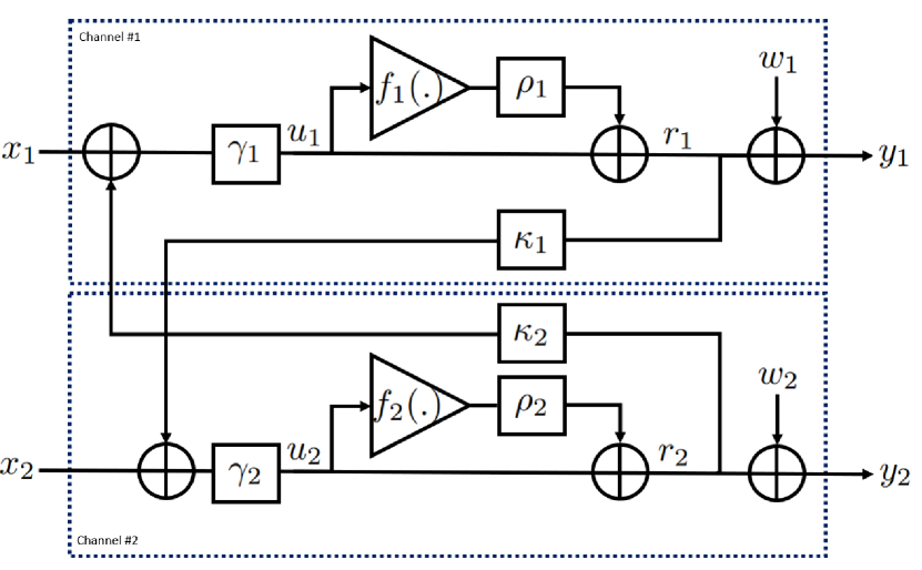
In this section, we derive a behavioral model of the 2×2222\times 2 MIMO transmitter with backward crosstalk shown in Fig. 1111Here the name “MIMO” refers to the hardware distortion model whose inputs and outputs are both related to the transmitter side. The inputs are the precoded signals and the outputs are the distorted signals to be transmitted.. In Fig. 1, the backward crosstalk is modeled by the parameters κ1subscript𝜅1\kappa_{1} and κ2subscript𝜅2\kappa_{2}. As mentioned above the backward crosstalk modeled in this way has two origins: crosstalk between in and output transmission lines, and the combination of output crosstalk and impedance mismatch. We have omitted the crosstalk from input to output. It is physically present due to reciprocity, but the contribution is small since it is not affected by the amplifier’s gain. We consider a symbol-sampled model where the outputs of the transmitter are denoted as y1,y2subscript𝑦1subscript𝑦2y_{1},y_{2}\in\mathbb{C}. The inputs of the transmitter are the OFDM modulated communication signals x1,x2subscript𝑥1subscript𝑥2x_{1},x_{2}\in\mathbb{C} [14], which are modeled as Gaussian distributed. All input signals have the same center frequency.
Refer to caption
Figure 1: A behavioral model of a 2×2222\times 2 MIMO transmitter with third-order polynomial nonlinearities f()subscript𝑓f_{\ell}(\cdot) with compression parameter ρsubscript𝜌\rho_{\ell}, subject to backward crosstalk via κsubscript𝜅\kappa_{\ell} and thermal noise wsubscript𝑤w_{\ell}.

Let 𝐱=(x1x2)T2×1𝐱superscriptsubscript𝑥1subscript𝑥2𝑇superscript21{\bf x}=(x_{1}\;x_{2})^{T}\in\mathbb{C}^{2\times 1} denote the inputs in vector form. When a MIMO transmitter is used for coherent beamforming, the inputs are correlated. To provide a general description, we therefore assume that 𝐱𝒩(𝟎,𝐂𝐱)similar-to𝐱subscript𝒩0subscript𝐂𝐱{\bf x}\sim\mathcal{N}_{\mathbb{C}}({\bf 0},{\bf C_{x}}), where 𝐂𝐱=𝔼[𝐱𝐱H]subscript𝐂𝐱𝔼delimited-[]superscript𝐱𝐱𝐻{\bf C_{x}}=\mathbb{E}[{\bf x}{\bf x}^{H}] denotes the covariance matrix. A general representation of 𝐂𝐱subscript𝐂𝐱{\bf C_{x}} is

𝐂𝐱=Px(1βξβξβ2),subscript𝐂𝐱subscript𝑃𝑥1𝛽𝜉𝛽superscript𝜉superscript𝛽2{\bf C_{x}}=P_{x}\left(\begin{array}[]{cc}1&\beta\xi\\ \beta\xi^{*}&\beta^{2}\end{array}\right), (1)

where the Px=𝔼[|x1|2]subscript𝑃𝑥𝔼delimited-[]superscriptsubscript𝑥12P_{x}=\mathbb{E}[|x_{1}|^{2}] is the power of the first input and it is taken as the reference power in the following parts of this paper. Moreover, β>0𝛽0\beta>0 is the square root of the ratio between the second signal’s power and the first signal’s power: β2=𝔼[|x2|2]/𝔼[|x1|2]superscript𝛽2𝔼delimited-[]superscriptsubscript𝑥22𝔼delimited-[]superscriptsubscript𝑥12\beta^{2}=\mathbb{E}[|x_{2}|^{2}]/\mathbb{E}[|x_{1}|^{2}]. The correlation coefficient of x1subscript𝑥1x_{1} and x2subscript𝑥2x_{2} is denoted by ξ𝜉\xi\in\mathbb{C} and satisfies |ξ|1𝜉1|\xi|\leq 1.

As shown in Fig. 1, the accessible transmitter output 𝐲=(y1y2)T2×1𝐲superscriptsubscript𝑦1subscript𝑦2𝑇superscript21{\bf y}=(y_{1}\;y_{2})^{T}\in\mathbb{C}^{2\times 1} is described by

𝐲=𝐫+𝐰,𝐲𝐫𝐰{\bf y}={\bf r}+{\bf w}, (2)

where 𝐫=(r1r2)T2×1𝐫superscriptsubscript𝑟1subscript𝑟2𝑇superscript21{\bf r}=(r_{1}\;r_{2})^{T}\in\mathbb{C}^{2\times 1} models the output from the power amplifiers and 𝐰=(w1w2)T𝒩(𝟎,σw2𝐈)𝐰superscriptsubscript𝑤1subscript𝑤2𝑇similar-tosubscript𝒩0superscriptsubscript𝜎𝑤2𝐈{\bf w}=(w_{1}\;w_{2})^{T}\sim\mathcal{N}_{\mathbb{C}}({\bf 0},\sigma_{w}^{2}\,{\bf I}) models the independent thermal noise that has variance σw2superscriptsubscript𝜎𝑤2\sigma_{w}^{2}.

II-A Bussgang Description of the Power Amplifier Output

The input to the \ellth power amplifier non-linearity is the internal amplified signal usubscript𝑢u_{\ell}\in\mathbb{C} and the output is rsubscript𝑟r_{\ell}\in\mathbb{C} for =1,212\ell=1,2. The input is an internal signal that is not equal to the amplified transmitter input γxsubscript𝛾subscript𝑥\gamma_{\ell}x_{\ell} when there is backward crosstalk. This is due to the feedback connection between antenna branches as illustrated in Fig. 1, i.e., the signal usubscript𝑢u_{\ell} represents the amplified version of the actual transmitter input, xsubscript𝑥x_{\ell}, plus the crosstalk signal that is coupled from the other antenna branch. We will model the backward crosstalk mathematically in Section II-B.

The \ellth power amplifier will ideally provide an amplification gain of γ>0subscript𝛾0\gamma_{\ell}>0, but has a nonlinear behavior determined by the compression parameter ρ0subscript𝜌0\rho_{\ell}\leq 0 and the function f()subscript𝑓f_{\ell}(\cdot). We assume that the power amplifiers are subject to third-order nonlinear distortion that compresses strong input signals, which implies f(u)=u|u|2subscript𝑓subscript𝑢subscript𝑢superscriptsubscript𝑢2f_{\ell}(u_{\ell})=u_{\ell}\,|u_{\ell}|^{2}. Hence, if usubscript𝑢u_{\ell} is the input to the \ellth amplifier, then the output is

r=u+ρf(u)=u+ρu|u|2,=1,2.formulae-sequencesubscript𝑟subscript𝑢subscript𝜌subscript𝑓subscript𝑢subscript𝑢subscript𝜌subscript𝑢superscriptsubscript𝑢212r_{\ell}=u_{\ell}+\rho_{\ell}\,f_{\ell}(u_{\ell})=u_{\ell}+\rho_{\ell}u_{\ell}\,|u_{\ell}|^{2},\quad\ell=1,2. (3)

The compression parameter values ρ1,ρ2subscript𝜌1subscript𝜌2\rho_{1},\rho_{2} are typically similar but nonidentical for the two branches. The vector signal 𝐫𝐫{\bf r} in (2) can then be expressed as

𝐫=𝐮+(ρ100ρ2)𝐆(u1|u1|2u2|u2|2)𝐟(𝐮),𝐫𝐮subscriptsubscript𝜌100subscript𝜌2absent𝐆subscriptsubscript𝑢1superscriptsubscript𝑢12missing-subexpressionsubscript𝑢2superscriptsubscript𝑢22missing-subexpressionabsent𝐟𝐮{\bf r}={\bf u}+\underbrace{\left(\begin{array}[]{cc}\rho_{1}&0\\ 0&\rho_{2}\end{array}\right)}_{\triangleq\displaystyle{\bf G}}\underbrace{\left(\begin{array}[]{cc}u_{1}\,|u_{1}|^{2}\\ u_{2}\,|u_{2}|^{2}\end{array}\right)}_{\triangleq\displaystyle{\bf f}({\bf u})}, (4)

where 𝐮=(u1u2)T𝐮superscriptsubscript𝑢1subscript𝑢2𝑇{\bf u}=(u_{1}\;u_{2})^{T} is the input to the nonlinearity. Note that in (4), the power amplifier output 𝐫𝐫{\bf r} is described as a function of the internal signal 𝐮𝐮{\bf u}, where 𝐮𝐮{\bf u} is a function of the transmitter gains, transmitter input 𝐱𝐱{\bf x} and the backward crosstalk via the power amplifier output 𝐫𝐫{\bf r}.

By Bussgang decomposition theory, the nonlinear transformation of the input 𝐮𝐮{\bf u} via 𝐟(𝐮)𝐟𝐮{\bf f}({\bf u}) in (4) can be equivalently described as

𝐫=𝐀𝐮+𝐯,𝐫𝐀𝐮𝐯{\bf r}={\bf A}\,{\bf u}+{\bf v}, (5)

where 𝐀𝐀{\bf A} is the constant Bussgang matrix and 𝐯𝐯{\bf v} is a zero-mean distortion term that is uncorrelated to the input 𝐮𝐮{\bf u} [14]. The observation bandwidth of 𝐫𝐫{\bf r} must be wide enough to comprise all spectral regrowth due to nonlinearities [20]. The Bussgang matrix 𝐀𝐀{\bf A} depends on both the properties of the input 𝐮𝐮{\bf u} exciting the nonlinearity and the nonlinearity 𝐟(𝐮)𝐟𝐮{\bf f}({\bf u}) itself. As shown in [16], it can be computed as 𝐀=𝔼[𝐫𝐮H](𝔼[𝐮𝐮H])1𝐀𝔼delimited-[]𝐫superscript𝐮𝐻superscript𝔼delimited-[]𝐮superscript𝐮𝐻1{\bf A}=\mathbb{E}[{\bf r}\,{\bf u}^{H}](\mathbb{E}[{\bf u}\,{\bf u}^{H}])^{-1} and by substituting (5) into this expression we obtain

𝐀=𝐈+𝐆𝐔¯𝐔1,𝐀𝐈𝐆¯𝐔superscript𝐔1{\bf A}={\bf I}+{\bf G}\,\overline{\bf U}\,{\bf U}^{-1}, (6)

where 𝐔𝔼[𝐮𝐮H]𝐔𝔼delimited-[]𝐮superscript𝐮𝐻{\bf U}\triangleq\mathbb{E}[{\bf u}\,{\bf u}^{H}] denotes the covariance matrix of 𝐮𝐮{\bf u} and 𝐔¯𝔼[𝐟(𝐮)𝐮H]¯𝐔𝔼delimited-[]𝐟𝐮superscript𝐮𝐻\overline{\bf U}\triangleq\mathbb{E}[{\bf f}({\bf u})\,{\bf u}^{H}] is a fourth-order moment matrix. Hence, the Bussgang matrix 𝐀𝐀{\bf A} in (6) depends on the transmitter model via 𝐆𝐆{\bf G} and the second- and fourth-order moments of the internal signal 𝐮𝐮{\bf u}, which are studied below. In addition, the properties of the power amplifier output 𝐫𝐫{\bf r} in (5) depends also on the nonlinear distortion noise 𝐯𝐯{\bf v} which is determined later.

II-B Modeling the Backward Crosstalk

We will now determine the power amplifier input 𝐮𝐮{\bf u} for the model in Fig. 1, where there is backward crosstalk between the transmission lines on the circuit board. This phenomenon is modeled by a feedback network, where

𝐮=(γ100γ2)𝐋𝐱+(0γ1κ2γ2κ10)𝐊𝐫.𝐮subscriptsubscript𝛾100subscript𝛾2absent𝐋𝐱subscript0subscript𝛾1subscript𝜅2subscript𝛾2subscript𝜅10absent𝐊𝐫{\bf u}=\underbrace{\left(\begin{array}[]{cc}\gamma_{1}&0\\ 0&\gamma_{2}\end{array}\right)}_{\triangleq\displaystyle{\bf L}}{\bf x}+\underbrace{\left(\begin{array}[]{cc}0&\gamma_{1}\,\kappa_{2}\\ \gamma_{2}\,\kappa_{1}&0\end{array}\right)}_{\triangleq\displaystyle{\bf K}}\,{\bf r}. (7)

Inserting (5) into (7) yields

𝐮=𝐋𝐱+𝐊(𝐀𝐮+𝐯).𝐮𝐋𝐱𝐊𝐀𝐮𝐯{\bf u}={\bf L}\,{\bf x}+{\bf K}({\bf A}\,{\bf u}+\,{\bf v}). (8)

By solving for 𝐮𝐮{\bf u}, the signal that excite the non-linearities is obtained as

𝐮=(𝐈𝐊𝐀)1(𝐋𝐱+𝐊𝐯).𝐮superscript𝐈𝐊𝐀1𝐋𝐱𝐊𝐯{\bf u}=({\bf I}-{\bf K}\,{\bf A})^{-1}\,({\bf L}\,{\bf x}+{\bf K}\,{\bf v}). (9)

This signal depends on the transmitter input 𝐱𝐱{\bf x}, the non-linear distortion noise 𝐯𝐯{\bf v}, and on the parameters of the considered transmitter model. We study these relationships in further detail in the following example.

II-B1 Linear Model and Transmitter Actual Gain

To focus on the impact of backward crosstalk, we will now exemplify a linear transmitter with 𝐆=𝟎𝐆0{\bf G}={\bf 0}, symmetric amplification γ=γ1=γ2𝛾subscript𝛾1subscript𝛾2\gamma=\gamma_{1}=\gamma_{2}, and a common backward crosstalk coefficient δ=γκ𝛿𝛾𝜅\delta=\gamma\,\kappa for which κ=κ1=κ2𝜅subscript𝜅1subscript𝜅2\kappa=\kappa_{1}=\kappa_{2}\in\mathbb{R} and |δ|<1𝛿1|\delta|<1. Then, according to (4), 𝐫=𝐮𝐫𝐮{\bf r}={\bf u}, and using (9) the power amplifier output becomes

𝐫𝐫\displaystyle{\bf r} =\displaystyle= 11δ2(1δδ1)(γ00γ)𝐱11superscript𝛿21𝛿𝛿1𝛾00𝛾𝐱\displaystyle\frac{1}{1-\delta^{2}}\left(\!\!\begin{array}[]{cc}1&\delta\\ \delta&1\end{array}\!\!\right)\left(\!\!\begin{array}[]{cc}\gamma&0\\ 0&\gamma\end{array}\!\!\right)\,{\bf x} (14)
=\displaystyle= 11δ2(γδγδγγ)𝐱.11superscript𝛿2𝛾𝛿𝛾𝛿𝛾𝛾𝐱\displaystyle\frac{1}{1-\delta^{2}}\left(\!\!\begin{array}[]{cc}\gamma&\delta\,\gamma\\ \delta\,\gamma&\gamma\end{array}\!\!\right)\,{\bf x}. (17)

Hence, the covariance matrix of 𝐫𝐫{\bf r} is

𝔼[𝐫𝐫H]=1(1δ2)2(γδγδγγ)𝐂𝐱(γδγδγγ).𝔼delimited-[]𝐫superscript𝐫𝐻1superscript1superscript𝛿22𝛾𝛿𝛾𝛿𝛾𝛾subscript𝐂𝐱𝛾𝛿𝛾𝛿𝛾𝛾\mathbb{E}[{\bf r}\,{\bf r}^{H}]=\frac{1}{(1-\delta^{2})^{2}}\left(\!\!\begin{array}[]{cc}\gamma&\delta\,\gamma\\ \delta\,\gamma&\gamma\end{array}\!\!\right){\bf C_{x}}\left(\!\!\begin{array}[]{cc}\gamma&\delta\,\gamma\\ \delta\,\gamma&\gamma\end{array}\!\!\right). (18)

In appropriately designed radio frequency transmitters, clearly the backward crosstalk yields small errors, that is |δ|1much-less-than𝛿1|\delta|\ll 1. As δ0𝛿0\delta\to 0, 𝔼[𝐫𝐫H]γ2𝐂𝐱𝔼delimited-[]𝐫superscript𝐫𝐻superscript𝛾2subscript𝐂𝐱\mathbb{E}[{\bf r}\,{\bf r}^{H}]\to\gamma^{2}{\bf C_{x}} and the transmitter only provides the amplification gain of γ𝛾\gamma. However, it is the case when |δ|𝛿|\delta| is small but non-zero that is of practical interest.

If the inputs are independent and symmetrically distributed, represented by 𝐂𝐱=Px𝐈subscript𝐂𝐱subscript𝑃𝑥𝐈{\bf C_{x}}=P_{x}\mathbf{I}, then for |δ|>0𝛿0|\delta|>0 we notice that (18) simplifies to

Px(1δ2)2(γ2(1+δ2)2δγ22δγ2γ2(1+δ2)).subscript𝑃𝑥superscript1superscript𝛿22superscript𝛾21superscript𝛿22𝛿superscript𝛾22𝛿superscript𝛾2superscript𝛾21superscript𝛿2\frac{P_{x}}{(1-\delta^{2})^{2}}\left(\!\!\begin{array}[]{cc}\gamma^{2}(1+\delta^{2})&2\delta\,\gamma^{2}\\ 2\delta\,\gamma^{2}&\gamma^{2}(1+\delta^{2})\end{array}\!\!\right). (19)

The non-zero off-diagonal elements in (19) show that the backward crosstalk makes the outputs correlated even when the inputs are uncorrelated. From (19), we also notice that the output power σr2=𝔼[|r|2]superscriptsubscript𝜎𝑟2𝔼delimited-[]superscriptsubscript𝑟2\sigma_{r\ell}^{2}=\mathbb{E}[|r_{\ell}|^{2}] of the \ellth output is

σr2=γ2(1+δ2)(1δ2)2Pxγ¯2Px,superscriptsubscript𝜎𝑟2superscript𝛾21superscript𝛿2superscript1superscript𝛿22subscript𝑃𝑥superscript¯𝛾2subscript𝑃𝑥\displaystyle\sigma_{r\ell}^{2}=\frac{\gamma^{2}\,(1+\delta^{2})}{(1-\delta^{2})^{2}}\,P_{x}\triangleq\bar{\gamma}^{2}\,P_{x}, (20)

where γ¯=γ1+δ2/(1δ2)¯𝛾𝛾1superscript𝛿21superscript𝛿2\bar{\gamma}=\gamma\sqrt{1+\delta^{2}}/(1-\delta^{2}) is the actual amplification gain of the transmitter. We have γ¯γsimilar-to-or-equals¯𝛾𝛾\bar{\gamma}\simeq\gamma for |δ|1much-less-than𝛿1|\delta|\ll 1, where similar-to-or-equals\simeq denotes an approximate expression where only the dominant terms are retained. Nevertheless, we want to further understand the small errors that also occur in the regime of |δ|1much-less-than𝛿1|\delta|\ll 1.

II-C Small-Error Analysis

In (9), we have derived that the internal signal 𝐮𝐮{\bf u} is a weighted sum of the input 𝐱𝐱{\bf x} and the non-linear distortion noise 𝐯𝐯{\bf v}, which is by construction uncorrelated to 𝐮𝐮\bf u. Although 𝐱𝐱{\bf x} was assumed to be Gaussian, the distortion noise 𝐯𝐯{\bf v} is non-Gaussian and also not independent of 𝐱𝐱{\bf x}, which makes an exact analysis cumbersome. In a small-error analysis where the distortion noise is negligible, the signal 𝐮𝐮{\bf u} in (9) can be approximated as

𝐮(𝐈𝐊𝐀)1𝐋𝐱.similar-to-or-equals𝐮superscript𝐈𝐊𝐀1𝐋𝐱{\bf u}\simeq({\bf I}-{\bf K}\,{\bf A})^{-1}\,{\bf L}\,{\bf x}. (21)

When the matrix representing the compression of power amplifiers, 𝐆𝐆{\bf G} is zero (i.e., the power amplifiers are ideal), the above approximation becomes exact. Note that this is a meaningful assumption when the power amplifiers operate close to the linear operation, which is possible with sufficient input power back-off. Furthermore, for a transmitter working close to its linear operation it holds that 𝐊𝐀𝐊similar-to-or-equals𝐊𝐀𝐊{\bf K}{\bf A}\simeq{\bf K} and |γ1γ2κ1κ2|1much-less-thansubscript𝛾1subscript𝛾2subscript𝜅1subscript𝜅21|\gamma_{1}\gamma_{2}\kappa_{1}\kappa_{2}|\ll 1, so that

𝐮(γ1γ1κ2γ2γ2κ1γ1γ2)𝐐𝐱.similar-to-or-equals𝐮subscriptsubscript𝛾1subscript𝛾1subscript𝜅2subscript𝛾2subscript𝛾2subscript𝜅1subscript𝛾1subscript𝛾2absent𝐐𝐱{\bf u}\simeq\underbrace{\left(\begin{array}[]{cc}\gamma_{1}&\gamma_{1}\,\kappa_{2}\,\gamma_{2}\\ \gamma_{2}\,\kappa_{1}\,\gamma_{1}&\gamma_{2}\end{array}\right)}_{\triangleq\displaystyle{\bf Q}}\,{\bf x}. (22)

From now on, we will utilize this approximate description, for which we can compute the Bussgang matrix 𝐀𝐀\mathbf{A} in closed form. The linear relation in (22) is based on two approximations: 1) the power amplifier operates close to its linear region, and 2) the power of the backward crosstalk is much smaller than the actual desired signal. These are all reasonable since the hardware is pre-calibrated to limit the distortion and only the small residual impairments remain to be modeled. In this paper, we analyze the system mathematically under these approximations and we then provide numerical simulations in Section V to demonstrate the accuracy.

From (22), we first notice that the internal signal 𝐮𝐮{\bf u} is now Gaussian distributed with covariance matrix 𝐔𝔼[𝐮𝐮H]𝐔𝔼delimited-[]𝐮superscript𝐮𝐻{\bf U}\triangleq\mathbb{E}[{\bf u}\,{\bf u}^{H}] given by

𝐔𝐔\displaystyle{\bf U} \displaystyle\triangleq (u11u12u12u22)=𝐐𝐂𝐱𝐐H,subscript𝑢11subscript𝑢12superscriptsubscript𝑢12subscript𝑢22𝐐subscript𝐂𝐱superscript𝐐𝐻\displaystyle\left(\begin{array}[]{cc}u_{11}&u_{12}\\ u_{12}^{*}&u_{22}\end{array}\right)={\bf Q}\,{\bf C_{x}}\,{\bf Q}^{H}, (25)

where the elements of 𝐔𝐔{\bf U} are denoted as

usubscript𝑢\displaystyle u_{\ell\ell} 𝔼[uu]=tPx,=1,2,formulae-sequenceabsent𝔼delimited-[]subscript𝑢superscriptsubscript𝑢subscript𝑡subscript𝑃𝑥12\displaystyle\triangleq\mathbb{E}[u_{\ell}\,u_{\ell}^{*}]=t_{\ell\ell}P_{x},\quad\ell=1,2, (26)
u12subscript𝑢12\displaystyle u_{12} 𝔼[u1u2]=t12Px,absent𝔼delimited-[]subscript𝑢1superscriptsubscript𝑢2subscript𝑡12subscript𝑃𝑥\displaystyle\triangleq\mathbb{E}[u_{1}\,u_{2}^{*}]=t_{12}P_{x},

where t11subscript𝑡11t_{11}, t12subscript𝑡12t_{12}, t22subscript𝑡22t_{22} can be computed as

t11subscript𝑡11\displaystyle t_{11} \displaystyle\triangleq γ12+2γ12γ2β{κ2ξ}+γ12γ22|κ2|2β2,superscriptsubscript𝛾122superscriptsubscript𝛾12subscript𝛾2𝛽superscriptsubscript𝜅2𝜉superscriptsubscript𝛾12superscriptsubscript𝛾22superscriptsubscript𝜅22superscript𝛽2\displaystyle\gamma_{1}^{2}+2\gamma_{1}^{2}\gamma_{2}\beta\Re\{\kappa_{2}^{*}\xi\}+\gamma_{1}^{2}\gamma_{2}^{2}|\kappa_{2}|^{2}\beta^{2}, (27)
t12subscript𝑡12\displaystyle t_{12} \displaystyle\triangleq γ1γ2(γ1κ1+βξ+γ1γ2κ1κ2βξ+γ2κ2β2),subscript𝛾1subscript𝛾2subscript𝛾1superscriptsubscript𝜅1𝛽𝜉subscript𝛾1subscript𝛾2superscriptsubscript𝜅1subscript𝜅2𝛽superscript𝜉subscript𝛾2subscript𝜅2superscript𝛽2\displaystyle\gamma_{1}\gamma_{2}\left(\gamma_{1}\kappa_{1}^{*}+\beta\xi+\gamma_{1}\gamma_{2}\kappa_{1}^{*}\kappa_{2}\beta\xi^{*}+\gamma_{2}\kappa_{2}\beta^{2}\right), (28)
t22subscript𝑡22\displaystyle t_{22} \displaystyle\triangleq γ22β2+2γ1γ22β{κ1ξ}+γ12γ22|κ1|2.superscriptsubscript𝛾22superscript𝛽22subscript𝛾1superscriptsubscript𝛾22𝛽subscript𝜅1𝜉superscriptsubscript𝛾12superscriptsubscript𝛾22superscriptsubscript𝜅12\displaystyle\gamma_{2}^{2}\beta^{2}+2\gamma_{1}\gamma_{2}^{2}\beta\Re\{\kappa_{1}\xi\}+\gamma_{1}^{2}\gamma_{2}^{2}|\kappa_{1}|^{2}. (29)

When the inputs to the non-linearity is Gaussian distributed, it follows that the Bussgang matrix 𝐀𝐀\mathbf{A} is diagonal [16, Sec. II.B] and given by

𝐀𝐀\displaystyle{\bf A} =(a100a2)=(𝔼[r1u1]𝔼[|u1|2]00𝔼[r2u2]𝔼[|u2|2])absentsubscript𝑎100subscript𝑎2𝔼delimited-[]subscript𝑟1superscriptsubscript𝑢1𝔼delimited-[]superscriptsubscript𝑢1200𝔼delimited-[]subscript𝑟2superscriptsubscript𝑢2𝔼delimited-[]superscriptsubscript𝑢22\displaystyle=\left(\!\!\begin{array}[]{cc}a_{1}&0\\ 0&a_{2}\end{array}\!\!\right)=\left(\!\!\begin{array}[]{cc}\frac{\mathbb{E}[r_{1}u_{1}^{*}]}{\mathbb{E}[|u_{1}|^{2}]}&0\\ 0&\frac{\mathbb{E}[r_{2}u_{2}^{*}]}{\mathbb{E}[|u_{2}|^{2}]}\end{array}\!\!\right) (34)
=(1+2ρ1u11001+2ρ2u22).absent12subscript𝜌1subscript𝑢110012subscript𝜌2subscript𝑢22\displaystyle=\left(\!\!\begin{array}[]{cc}1+2\rho_{1}u_{11}&0\\ 0&1+2\rho_{2}u_{22}\end{array}\!\!\right). (37)

This result alternatively can be obtained by the first part of Appendix A. Since ρ1,ρ2subscript𝜌1subscript𝜌2\rho_{1},\rho_{2} are negative parameters, the diagonal elements of 𝐀𝐀\mathbf{A} will be smaller than one. For practical parameter values it holds that 0<|1+2ρu|<1012subscript𝜌subscript𝑢10<|1+2\rho_{\ell}u_{\ell\ell}|<1, for =1,212\ell=1,2, thus when substituting (37) into (5), the output of the nonlinearity is the input with reduced gain plus the nonlinear distortion noise. We call 1+2ρu12subscript𝜌subscript𝑢1+2\rho_{\ell}u_{\ell\ell} the Bussgang attenuation.

II-D Transmitter Output Error

We will now utilize the Bussgang decomposition in (5), the closed-form results in the small-error regime, and the obtained properties of the internal signal 𝐮𝐮{\bf u} to derive properties of the transmitter output error. These properties are key to analyze the end performance of the transmitter.

The transmitter output 𝐲𝐲{\bf y} in (2) is now given as functions of the transmitter input 𝐱𝐱{\bf x}, nonlinear distortion noise 𝐯𝐯{\bf v}, and transmitter thermal noise 𝐰𝐰{\bf w} by

𝐲=𝐀𝐐𝐱+𝐯+𝐰,𝐲𝐀𝐐𝐱𝐯𝐰{\bf y}={\bf A}\,{\bf Q}\,{\bf x}+{\bf v}+{\bf w}, (38)

where (5) and (22) were used to form an expression of the input 𝐱𝐱{\bf x} and nonlinear distortion noise 𝐯𝐯{\bf v}. In (38), 𝐐𝐐{\bf Q} is given in (22) and the matrix 𝐀𝐀{\bf A} in (37). The ideal output 𝐲osubscript𝐲o{\bf y}_{\mbox{\scriptsize o}} of the transmitter is given by the purely amplified inputs, that is

𝐲o=(yo1yo2)𝐋𝐱,subscript𝐲osubscript𝑦o1subscript𝑦o2𝐋𝐱{\bf y}_{\mbox{\scriptsize o}}=\left(\begin{array}[]{c}y_{\mbox{\scriptsize o}1}\\ y_{\mbox{\scriptsize o}2}\end{array}\right)\triangleq{\bf L}\,{\bf x}, (39)

where the gain matrix 𝐋𝐋{\bf L} is defined in (7). From (38) and (39), the error signal 𝐞𝐞{\bf e} determining the full properties of the 2×2222\times 2 MIMO transmitter reads

𝐞𝐲𝐲o=(𝐀𝐐𝐋)𝐱𝐱~+𝐯+𝐰.𝐞𝐲subscript𝐲osubscript𝐀𝐐𝐋𝐱absent~𝐱𝐯𝐰{\bf e}\triangleq{\bf y}-{\bf y}_{\mbox{\scriptsize o}}=\underbrace{({\bf A}\,{\bf Q}-{\bf L})\,{\bf x}}_{\triangleq\displaystyle\widetilde{{\bf x}}}+{\bf v}+{\bf w}. (40)

The introduced signal 𝐱~~𝐱\widetilde{{\bf x}} captures (the linear part of) the error due to backward crosstalk and Bussgang attenuation, 𝐯𝐯{\bf v} is the nonlinear distortion noise, and 𝐰𝐰{\bf w} is the thermal noise. The model (40) of the transmitter output error 𝐞𝐞{\bf e} forms the basis for the performance analysis in the following sections.

III Performance Analysis Based on the NMSE

One way to measure the transmitter performance is to measure the NMSE between the ideal output 𝐲osubscript𝐲o{\bf y}_{\mbox{\scriptsize o}} in (39) and the true output in (38). This is the normalized power of the error vector in (40). The three error terms defining the total error in (40) are jointly uncorrelated. Accordingly, the error covariance 𝐄=𝔼[𝐞𝐞H]𝐄𝔼delimited-[]𝐞superscript𝐞𝐻{\bf E}=\mathbb{E}[{\bf e}\,{\bf e}^{H}] can be written as

𝐄=𝐗~+𝐕+σw2𝐈,𝐄~𝐗𝐕superscriptsubscript𝜎𝑤2𝐈{\bf E}=\widetilde{{\bf X}}+{\bf V}+\sigma_{w}^{2}\,{\bf I}, (41)

where the covariance matrices 𝐗~=𝔼[𝐱~𝐱~H]~𝐗𝔼delimited-[]~𝐱superscript~𝐱𝐻\widetilde{{\bf X}}=\mathbb{E}[\widetilde{{\bf x}}\,\widetilde{{\bf x}}^{H}] and 𝐕=𝔼[𝐯𝐯H]𝐕𝔼delimited-[]𝐯superscript𝐯𝐻{\bf V}=\mathbb{E}[{\bf v}\,{\bf v}^{H}] are to be determined, while σw2superscriptsubscript𝜎𝑤2\sigma_{w}^{2} still denotes the variance of the thermal noise.

III-A Properties of the Linear Error Matrix 𝐗~~𝐗\widetilde{{\bf X}}

From (40) it follows that the covariance matrix 𝐗~~𝐗\widetilde{{\bf X}} in (41) reads

𝐗~=(𝐀𝐐𝐋)𝐂𝐱(𝐀𝐐𝐋)H,~𝐗𝐀𝐐𝐋subscript𝐂𝐱superscript𝐀𝐐𝐋𝐻\widetilde{{\bf X}}=({\bf A}\,{\bf Q}-{\bf L}){\bf C_{x}}({\bf A}\,{\bf Q}-{\bf L})^{H}, (42)

where 𝔼[𝐱𝐱H]=𝐂𝐱𝔼delimited-[]𝐱superscript𝐱𝐻subscript𝐂𝐱\mathbb{E}[{\bf x}\,{\bf x}^{H}]={\bf C_{x}} was used. It follows from a straightforward calculation using 𝐀𝐀{\bf A} in (37), 𝐐𝐐{\bf Q} in (22), and 𝐋𝐋{\bf L} in (7) that

𝐀𝐐𝐋=(2γ1ρ1u11γ1κ2γ2(1+2ρ1u11)γ2κ1γ1(1+2ρ2u22)2γ2ρ2u22),𝐀𝐐𝐋2subscript𝛾1subscript𝜌1subscript𝑢11subscript𝛾1subscript𝜅2subscript𝛾212subscript𝜌1subscript𝑢11subscript𝛾2subscript𝜅1subscript𝛾112subscript𝜌2subscript𝑢222subscript𝛾2subscript𝜌2subscript𝑢22{\bf A}\,{\bf Q}-{\bf L}=\left(\!\!\begin{array}[]{cc}2\gamma_{1}\,\rho_{1}\,u_{11}&\gamma_{1}\,\kappa_{2}\,\gamma_{2}(1+2\rho_{1}u_{11})\\ \gamma_{2}\,\kappa_{1}\,\gamma_{1}(1+2\rho_{2}u_{22})&2\gamma_{2}\,\rho_{2}\,u_{22}\end{array}\!\!\right), (43)

where the result in (43) is expressed in terms of the intermediate diagonal elements of 𝐔𝐔{\bf U} in (25), and the transmitter parameters. We can also express 𝐀𝐐𝐋𝐀𝐐𝐋{\bf A}{\bf Q}-{\bf L} as

𝐀𝐐𝐋=2𝐆𝐁𝐐+𝐊𝐋,𝐀𝐐𝐋2𝐆𝐁𝐐𝐊𝐋{\bf A}{\bf Q}-{\bf L}=2{\bf G}{\bf B}{\bf Q}+{\bf K}{\bf L}, (44)

where 𝐊𝐊{\bf K} is defined in (7) and 𝐁𝐁{\bf B} is defined as

𝐁(u1100u22).𝐁subscript𝑢1100subscript𝑢22{\bf B}\triangleq\left(\begin{array}[]{cc}u_{11}&0\\ 0&u_{22}\end{array}\right). (45)

Using (25) and (44), the covariance matrix 𝐗~~𝐗\widetilde{{\bf X}} in (42) reads

𝐗~~𝐗\displaystyle\widetilde{{\bf X}} =\displaystyle= 4𝐆𝐁𝐔𝐁𝐆+𝐊𝐋𝐂𝐱𝐋𝐊H4𝐆𝐁𝐔𝐁𝐆subscript𝐊𝐋𝐂𝐱superscript𝐋𝐊𝐻\displaystyle 4{\bf G}{\bf B}{\bf U}{\bf B}{\bf G}+{\bf K}{\bf L}{\bf C_{x}}{\bf L}{\bf K}^{H} (46)
+2𝐊𝐋𝐂𝐱𝐐H𝐁𝐆+2𝐆𝐁𝐐𝐂𝐱𝐋𝐊H.2subscript𝐊𝐋𝐂𝐱superscript𝐐𝐻𝐁𝐆2subscript𝐆𝐁𝐐𝐂𝐱superscript𝐋𝐊𝐻\displaystyle+2{\bf K}{\bf L}{\bf C_{x}}{\bf Q}^{H}{\bf B}{\bf G}+2{\bf G}{\bf B}{\bf Q}{\bf C_{x}}{\bf L}{\bf K}^{H}.

If the elements of 𝐗~~𝐗\widetilde{{\bf X}} are denoted as

𝐗~(x~11x~12x~12x~22),~𝐗subscript~𝑥11subscript~𝑥12superscriptsubscript~𝑥12subscript~𝑥22\widetilde{{\bf X}}\triangleq\left(\begin{array}[]{cc}\tilde{x}_{11}&\tilde{x}_{12}\\ \tilde{x}_{12}^{*}&\tilde{x}_{22}\end{array}\right), (47)

then a straightforward calculation provides

x~11subscript~𝑥11\displaystyle\tilde{x}_{11} =\displaystyle= 4ρ12t113Px3+4γ12γ2t11ρ1(γ2β2|κ2|2+β{κ2ξ})Px24superscriptsubscript𝜌12superscriptsubscript𝑡113superscriptsubscript𝑃𝑥34superscriptsubscript𝛾12subscript𝛾2subscript𝑡11subscript𝜌1subscript𝛾2superscript𝛽2superscriptsubscript𝜅22𝛽subscript𝜅2superscript𝜉superscriptsubscript𝑃𝑥2\displaystyle 4\rho_{1}^{2}\,t_{11}^{3}\,P_{x}^{3}+4\gamma_{1}^{2}\gamma_{2}t_{11}\rho_{1}\left(\gamma_{2}\beta^{2}\left|\kappa_{2}\right|^{2}+\beta\Re\left\{\kappa_{2}\xi^{*}\right\}\right)P_{x}^{2} (48)
+β2γ12γ22|κ2|2Px,superscript𝛽2superscriptsubscript𝛾12superscriptsubscript𝛾22superscriptsubscript𝜅22subscript𝑃𝑥\displaystyle+\beta^{2}\gamma_{1}^{2}\gamma_{2}^{2}|\kappa_{2}|^{2}P_{x},
x~12subscript~𝑥12\displaystyle\tilde{x}_{12} =\displaystyle= 4ρ1ρ2t12t11t22Px3+2γ12γ2t11ρ1κ1(1+γ2βξκ2)Px24subscript𝜌1subscript𝜌2subscript𝑡12subscript𝑡11subscript𝑡22superscriptsubscript𝑃𝑥32superscriptsubscript𝛾12subscript𝛾2subscript𝑡11subscript𝜌1superscriptsubscript𝜅11subscript𝛾2𝛽superscript𝜉subscript𝜅2superscriptsubscript𝑃𝑥2\displaystyle 4\rho_{1}\,\rho_{2}\,t_{12}\,t_{11}\,t_{22}\,P_{x}^{3}+2\gamma_{1}^{2}\gamma_{2}t_{11}\rho_{1}\kappa_{1}^{*}\left(1+\gamma_{2}\beta\xi^{*}\kappa_{2}\right)P_{x}^{2} (49)
+2γ1γ22t22ρ2κ2(β2+γ1βξκ1)Px22subscript𝛾1superscriptsubscript𝛾22subscript𝑡22subscript𝜌2subscript𝜅2superscript𝛽2subscript𝛾1𝛽superscript𝜉superscriptsubscript𝜅1superscriptsubscript𝑃𝑥2\displaystyle+2\gamma_{1}\gamma_{2}^{2}t_{22}\rho_{2}\kappa_{2}\left(\beta^{2}+\gamma_{1}\beta\xi^{*}\kappa_{1}^{*}\right)P_{x}^{2}
+βξγ12γ22κ1κ2Px,𝛽superscript𝜉superscriptsubscript𝛾12superscriptsubscript𝛾22superscriptsubscript𝜅1subscript𝜅2subscript𝑃𝑥\displaystyle+\beta\xi^{*}\gamma_{1}^{2}\gamma_{2}^{2}\kappa_{1}^{*}\kappa_{2}P_{x},
x~22subscript~𝑥22\displaystyle\tilde{x}_{22} =\displaystyle= 4ρ22t223Px3+4γ1γ22t22ρ2(γ1|κ1|2+β{κ1ξ})Px24superscriptsubscript𝜌22superscriptsubscript𝑡223superscriptsubscript𝑃𝑥34subscript𝛾1superscriptsubscript𝛾22subscript𝑡22subscript𝜌2subscript𝛾1superscriptsubscript𝜅12𝛽subscript𝜅1𝜉superscriptsubscript𝑃𝑥2\displaystyle 4\rho_{2}^{2}\,t_{22}^{3}\,P_{x}^{3}+4\gamma_{1}\gamma_{2}^{2}t_{22}\rho_{2}\left(\gamma_{1}\left|\kappa_{1}\right|^{2}+\beta\Re\left\{\kappa_{1}\xi\right\}\right)P_{x}^{2} (50)
+γ12γ22|κ1|2Px.superscriptsubscript𝛾12superscriptsubscript𝛾22superscriptsubscript𝜅12subscript𝑃𝑥\displaystyle+\gamma_{1}^{2}\gamma_{2}^{2}|\kappa_{1}|^{2}P_{x}.

In the above equations, the results are compactly expressed in terms of the input signal and transmitter hardware parameters. Note that all the terms in (48)-(50) are third-order polynomials of the reference input power Pxsubscript𝑃𝑥P_{x}. The result above will be used to derive the error covariance in (41), once the elements of 𝐕𝐕{\bf V} have been determined.

III-B Properties of the Nonlinear Error Matrix 𝐕𝐕{\bf V}

The covariance matrix of the distortion noise 𝐯𝐯{\bf v} is known to be [14]

𝐕=𝐆(𝐔¯¯𝐔¯𝐔1𝐔¯H)𝐆H,𝐕𝐆¯¯𝐔¯𝐔superscript𝐔1superscript¯𝐔𝐻superscript𝐆𝐻{\bf V}={\bf G}\,(\overline{\overline{\bf U}}-\overline{\bf U}\,{\bf U}^{-1}\,\overline{\bf U}^{H})\,{\bf G}^{H}, (51)

where 𝐆𝐆{\bf G} is given in (4) and 𝐔¯¯=𝔼[𝐟(𝐮)𝐟(𝐮)H]¯¯𝐔𝔼delimited-[]𝐟𝐮𝐟superscript𝐮𝐻\overline{\overline{\bf U}}=\mathbb{E}[{\bf f}({\bf u})\,{\bf f}({\bf u})^{H}] is the matrix of higher-order moments. It is shown in Appendix A that (51) can be reduced to

𝐕=2𝐆𝐂𝐆H,𝐕2𝐆𝐂superscript𝐆𝐻{\bf V}=2\,{\bf G}\,{\bf C}\,{\bf G}^{H}, (52)

where the matrix 𝐂𝐂{\bf C} can be compactly written using the properties of the internal signal 𝐮𝐮{\bf u}:

𝐂=(u113u12|u12|2u12|u12|2u223).𝐂superscriptsubscript𝑢113subscript𝑢12superscriptsubscript𝑢122superscriptsubscript𝑢12superscriptsubscript𝑢122superscriptsubscript𝑢223\displaystyle{\bf C}=\left(\begin{array}[]{cc}u_{11}^{3}&u_{12}\,|u_{12}|^{2}\\ u_{12}^{*}\,|u_{12}|^{2}&u_{22}^{3}\end{array}\right). (55)

With (52) and (55) as starting point, a straightforward calculation reveals that the covariance matrix 𝐕𝐕{\bf V} in (51) reads

𝐕(v11v12v12v22),𝐕subscript𝑣11subscript𝑣12superscriptsubscript𝑣12subscript𝑣22{\bf V}\triangleq\left(\begin{array}[]{cc}v_{11}&v_{12}\\ v_{12}^{*}&v_{22}\end{array}\right), (56)

where

vsubscript𝑣\displaystyle v_{\ell\ell} =\displaystyle= 2ρ2u3=2ρ2t3Px3,=1,2,formulae-sequence2superscriptsubscript𝜌2superscriptsubscript𝑢32superscriptsubscript𝜌2superscriptsubscript𝑡3superscriptsubscript𝑃𝑥312\displaystyle 2\rho_{\ell}^{2}\,u_{\ell\ell}^{3}=2\rho_{\ell}^{2}t_{\ell\ell}^{3}P_{x}^{3},\quad\ell=1,2, (57)
v12subscript𝑣12\displaystyle v_{12} =\displaystyle= 2ρ1ρ2u12|u12|2=2ρ1ρ2t12|t12|2Px3.2subscript𝜌1subscript𝜌2subscript𝑢12superscriptsubscript𝑢1222subscript𝜌1subscript𝜌2subscript𝑡12superscriptsubscript𝑡122superscriptsubscript𝑃𝑥3\displaystyle 2\rho_{1}\,\rho_{2}\,u_{12}\,|u_{12}|^{2}=2\rho_{1}\rho_{2}t_{12}|t_{12}|^{2}P_{x}^{3}. (58)

III-C Closed-form Expressions for the NMSE

By denoting the diagonal elements of the error covariance 𝐄𝐄{\bf E} in (41) as e11subscript𝑒11e_{11}, e22subscript𝑒22e_{22}, the figure-of-merit NMSE for the first and second branch is given as

NMSE1subscriptNMSE1\displaystyle{\mbox{NMSE}}_{1} \displaystyle\triangleq e11𝔼{|yo1|2}=e11γ12Px,subscript𝑒11𝔼superscriptsubscript𝑦o12subscript𝑒11superscriptsubscript𝛾12subscript𝑃𝑥\displaystyle\frac{e_{11}}{\mathbb{E}\{|y_{\mbox{\scriptsize o}1}|^{2}\}}=\frac{e_{11}}{\gamma_{1}^{2}\,P_{x}}, (59)
NMSE2subscriptNMSE2\displaystyle{\mbox{NMSE}}_{2} \displaystyle\triangleq e22𝔼{|yo2|2}=e22γ22β2Px.subscript𝑒22𝔼superscriptsubscript𝑦o22subscript𝑒22superscriptsubscript𝛾22superscript𝛽2subscript𝑃𝑥\displaystyle\frac{e_{22}}{\mathbb{E}\{|y_{\mbox{\scriptsize o}2}|^{2}\}}=\frac{e_{22}}{\gamma_{2}^{2}\,\beta^{2}\,P_{x}}. (60)

By utilizing the expressions derived in (48), (50), (57), the diagonal elements e11subscript𝑒11e_{11} and e22subscript𝑒22e_{22} are obtained as

e11subscript𝑒11\displaystyle e_{11} =\displaystyle= x~11+v11+σw2subscript~𝑥11subscript𝑣11superscriptsubscript𝜎𝑤2\displaystyle\tilde{x}_{11}+v_{11}+\sigma_{w}^{2} (61)
=\displaystyle= 6ρ12t113Px3+4γ12γ2t11ρ1(γ2β2|κ2|2+β{κ2ξ})Px26superscriptsubscript𝜌12superscriptsubscript𝑡113superscriptsubscript𝑃𝑥34superscriptsubscript𝛾12subscript𝛾2subscript𝑡11subscript𝜌1subscript𝛾2superscript𝛽2superscriptsubscript𝜅22𝛽subscript𝜅2superscript𝜉superscriptsubscript𝑃𝑥2\displaystyle 6\rho_{1}^{2}\,t_{11}^{3}\,P_{x}^{3}+4\gamma_{1}^{2}\gamma_{2}t_{11}\rho_{1}\left(\gamma_{2}\beta^{2}\left|\kappa_{2}\right|^{2}+\beta\Re\left\{\kappa_{2}\xi^{*}\right\}\right)P_{x}^{2}
+β2γ12γ22|κ2|2Px+σw2,superscript𝛽2superscriptsubscript𝛾12superscriptsubscript𝛾22superscriptsubscript𝜅22subscript𝑃𝑥superscriptsubscript𝜎𝑤2\displaystyle+\beta^{2}\gamma_{1}^{2}\gamma_{2}^{2}|\kappa_{2}|^{2}P_{x}+\sigma_{w}^{2},
e22subscript𝑒22\displaystyle e_{22} =\displaystyle= x~22+v22+σw2subscript~𝑥22subscript𝑣22superscriptsubscript𝜎𝑤2\displaystyle\tilde{x}_{22}+v_{22}+\sigma_{w}^{2} (62)
=\displaystyle= 6ρ22t223Px3+4γ1γ22t22ρ2(γ1|κ1|2+β{κ1ξ})Px26superscriptsubscript𝜌22superscriptsubscript𝑡223superscriptsubscript𝑃𝑥34subscript𝛾1superscriptsubscript𝛾22subscript𝑡22subscript𝜌2subscript𝛾1superscriptsubscript𝜅12𝛽subscript𝜅1𝜉superscriptsubscript𝑃𝑥2\displaystyle 6\rho_{2}^{2}\,t_{22}^{3}\,P_{x}^{3}+4\gamma_{1}\gamma_{2}^{2}t_{22}\rho_{2}\left(\gamma_{1}\left|\kappa_{1}\right|^{2}+\beta\Re\left\{\kappa_{1}\xi\right\}\right)P_{x}^{2}
+γ12γ22|κ1|2Px+σw2.superscriptsubscript𝛾12superscriptsubscript𝛾22superscriptsubscript𝜅12subscript𝑃𝑥superscriptsubscript𝜎𝑤2\displaystyle+\gamma_{1}^{2}\gamma_{2}^{2}|\kappa_{1}|^{2}P_{x}+\sigma_{w}^{2}.

With the variances e11subscript𝑒11e_{11} and e22subscript𝑒22e_{22} of the first and second branch errors in (61)-(62), NMSE1subscriptNMSE1{\mbox{NMSE}}_{1} and NMSE2subscriptNMSE2{\mbox{NMSE}}_{2} becomes

NMSE1subscriptNMSE1\displaystyle{\mbox{NMSE}}_{1} =\displaystyle= 6ρ12t113γ12Px26superscriptsubscript𝜌12superscriptsubscript𝑡113superscriptsubscript𝛾12superscriptsubscript𝑃𝑥2\displaystyle\frac{6\rho_{1}^{2}\,t_{11}^{3}}{\gamma_{1}^{2}}\,P_{x}^{2} (63)
+4γ2t11ρ1(γ2β2|κ2|2+β{κ2ξ})Px4subscript𝛾2subscript𝑡11subscript𝜌1subscript𝛾2superscript𝛽2superscriptsubscript𝜅22𝛽subscript𝜅2superscript𝜉subscript𝑃𝑥\displaystyle+4\gamma_{2}t_{11}\rho_{1}\left(\gamma_{2}\beta^{2}\left|\kappa_{2}\right|^{2}+\beta\Re\left\{\kappa_{2}\xi^{*}\right\}\right)P_{x}
+β2γ22|κ2|2+σw2γ12Px,superscript𝛽2superscriptsubscript𝛾22superscriptsubscript𝜅22superscriptsubscript𝜎𝑤2superscriptsubscript𝛾12subscript𝑃𝑥\displaystyle+\beta^{2}\gamma_{2}^{2}|\kappa_{2}|^{2}+\frac{\sigma_{w}^{2}}{\gamma_{1}^{2}\,P_{x}},
NMSE2subscriptNMSE2\displaystyle{\mbox{NMSE}}_{2} =\displaystyle= 6ρ22t223γ22β2Px26superscriptsubscript𝜌22superscriptsubscript𝑡223superscriptsubscript𝛾22superscript𝛽2superscriptsubscript𝑃𝑥2\displaystyle\frac{6\rho_{2}^{2}\,t_{22}^{3}}{\gamma_{2}^{2}\beta^{2}}\,P_{x}^{2} (64)
+4γ1t22ρ2β2(γ1|κ1|2+β{κ1ξ})Px4subscript𝛾1subscript𝑡22subscript𝜌2superscript𝛽2subscript𝛾1superscriptsubscript𝜅12𝛽subscript𝜅1𝜉subscript𝑃𝑥\displaystyle+\frac{4\gamma_{1}t_{22}\rho_{2}}{\beta^{2}}\left(\gamma_{1}\left|\kappa_{1}\right|^{2}+\beta\Re\left\{\kappa_{1}\xi\right\}\right)P_{x}
+γ12|κ1|2β2+σw2γ22β2Px.superscriptsubscript𝛾12superscriptsubscript𝜅12superscript𝛽2superscriptsubscript𝜎𝑤2superscriptsubscript𝛾22superscript𝛽2subscript𝑃𝑥\displaystyle+\gamma_{1}^{2}\frac{|\kappa_{1}|^{2}}{\beta^{2}}+\frac{\sigma_{w}^{2}}{\gamma_{2}^{2}\,\beta^{2}P_{x}}.
Lemma 1

The NMSEs for the two antenna branches, NMSE1subscriptNMSE1{\mbox{NMSE}}_{1} and NMSE2subscriptNMSE2{\mbox{NMSE}}_{2}, are convex functions of the reference input power Pxsubscript𝑃𝑥P_{x} for Px0subscript𝑃𝑥0P_{x}\geq 0.

Proof:

This can easily be proved by taking the second derivative of NMSE1(Px)subscriptNMSE1subscript𝑃𝑥{\mbox{NMSE}}_{1}(P_{x}) and NMSE2(Px)subscriptNMSE2subscript𝑃𝑥{\mbox{NMSE}}_{2}(P_{x}) with respect to Pxsubscript𝑃𝑥P_{x} and show that they are positive. Direct differentiation yields

NMSE1′′(Px)=12ρ12t113γ12+2σw2γ12Px3,superscriptsubscriptNMSE1′′subscript𝑃𝑥12superscriptsubscript𝜌12superscriptsubscript𝑡113superscriptsubscript𝛾122superscriptsubscript𝜎𝑤2superscriptsubscript𝛾12superscriptsubscript𝑃𝑥3\displaystyle{\mbox{NMSE}}_{1}^{\prime\prime}(P_{x})=\frac{12\rho_{1}^{2}\,t_{11}^{3}}{\gamma_{1}^{2}}+\frac{2\sigma_{w}^{2}}{\gamma_{1}^{2}\,P_{x}^{3}},
NMSE2′′(Px)=12ρ22t223γ22β2+2σw2γ22β2Px3.superscriptsubscriptNMSE2′′subscript𝑃𝑥12superscriptsubscript𝜌22superscriptsubscript𝑡223superscriptsubscript𝛾22superscript𝛽22superscriptsubscript𝜎𝑤2superscriptsubscript𝛾22superscript𝛽2superscriptsubscript𝑃𝑥3\displaystyle{\mbox{NMSE}}_{2}^{\prime\prime}(P_{x})=\frac{12\rho_{2}^{2}\,t_{22}^{3}}{\gamma_{2}^{2}\beta^{2}}+\frac{2\sigma_{w}^{2}}{\gamma_{2}^{2}\,\beta^{2}P_{x}^{3}}. (65)

Both are positive for Px0subscript𝑃𝑥0P_{x}\geq 0 which is the range of interest. ∎

The closed-form NMSE expressions in (63) and (64) provide insights into the hardware behavior. Let us focus on NMSE1subscriptNMSE1{\mbox{NMSE}}_{1} since the other branch has identical characteristics, except for the different notation. If we assume that the strength of the backward crosstalk signal is very small compared to the main signal, we have γ2|κ2|1much-less-thansubscript𝛾2subscript𝜅21\gamma_{2}\left|\kappa_{2}\right|\ll 1 and t11subscript𝑡11t_{11} in (27) can be approximated as t11γ12similar-to-or-equalssubscript𝑡11superscriptsubscript𝛾12t_{11}\simeq\gamma_{1}^{2} and furthermore NMSE1subscriptNMSE1{\mbox{NMSE}}_{1} can be approximated as

NMSE16ρ12γ14Px2+4ρ1βγ2{κ2ξ}γ12Px+σw2γ12Px.similar-to-or-equalssubscriptNMSE16superscriptsubscript𝜌12superscriptsubscript𝛾14superscriptsubscript𝑃𝑥24subscript𝜌1𝛽subscript𝛾2subscript𝜅2superscript𝜉superscriptsubscript𝛾12subscript𝑃𝑥superscriptsubscript𝜎𝑤2superscriptsubscript𝛾12subscript𝑃𝑥\displaystyle{\mbox{NMSE}}_{1}\simeq 6\rho_{1}^{2}\gamma_{1}^{4}\,P_{x}^{2}+4\rho_{1}\beta\gamma_{2}\Re\left\{\kappa_{2}\xi^{*}\right\}\gamma_{1}^{2}P_{x}+\frac{\sigma_{w}^{2}}{\gamma_{1}^{2}\,P_{x}}. (66)

We note that it is a convex function of the ideal amplified signal power 𝔼{|yo1|2}=γ12Px𝔼superscriptsubscript𝑦o12superscriptsubscript𝛾12subscript𝑃𝑥\mathbb{E}\{|y_{\mbox{\scriptsize o}1}|^{2}\}=\gamma_{1}^{2}P_{x}. This means that when the desired amplifier gain of the first transmitter branch, γ1subscript𝛾1\gamma_{1} increases, the input reference power Pxsubscript𝑃𝑥P_{x} should be decreased at the same ratio with γ12superscriptsubscript𝛾12\gamma_{1}^{2} in order to keep the NMSE the same. Moreover, the first term in (66) is a monotonically increasing function of Pxsubscript𝑃𝑥P_{x} and as the compression ratio of the first branch’s power amplifier, |ρ1|subscript𝜌1|\rho_{1}|, increases, it increases with the square of it. Note that this term dominates the NMSE when γ12Pxsuperscriptsubscript𝛾12subscript𝑃𝑥\gamma_{1}^{2}P_{x} grows. The sign of the second term is dependent on {κ2ξ}subscript𝜅2superscript𝜉\Re\left\{\kappa_{2}\xi^{*}\right\}. Since ρ10subscript𝜌10\rho_{1}\leq 0, when the crosstalk parameter κ2subscript𝜅2\kappa_{2} and the correlation coefficient ξ𝜉\xi are phase-aligned, this term reduces the NMSE to some extent. In this case, the power amplifier non-linearity corresponding to the first term is the main source for the distortion. When {κ2ξ}<0subscript𝜅2superscript𝜉0\Re\left\{\kappa_{2}\xi^{*}\right\}<0, the sum of the first two terms monotonically increases with Pxsubscript𝑃𝑥P_{x} and we see a combination of power amplifer and backward crosstalk distortion. In this case, the last term regularizes the NMSE since it decreases with Pxsubscript𝑃𝑥P_{x} and goes to infinity as Px0subscript𝑃𝑥0P_{x}\to 0, hence the optimal input reference power is clearly non-zero. This term dominates the NMSE expression when Pxsubscript𝑃𝑥P_{x} is small compared to the thermal noise variance.

III-D Power Back-off for Minimizing Maximum NMSE

As discussed above, the NMSE of an antenna branch is minimized at a non-zero value of Pxsubscript𝑃𝑥P_{x}. For a single-antenna transceiver, there is only one NMSE and therefore it is desirable to find the average input power that minimizes its NMSE. We can study that special case by setting β=0𝛽0\beta=0, we obtain NMSE1=6ρ12γ14Px2+σw2γ12PxsubscriptNMSE16superscriptsubscript𝜌12superscriptsubscript𝛾14superscriptsubscript𝑃𝑥2superscriptsubscript𝜎𝑤2superscriptsubscript𝛾12subscript𝑃𝑥{\mbox{NMSE}}_{1}=6\rho_{1}^{2}\,\gamma_{1}^{4}\,P_{x}^{2}+\frac{\sigma_{w}^{2}}{\gamma_{1}^{2}\,P_{x}} from (63). It is then straightforward to show that it is minimized by

Px=1γ12σw212ρ123,subscript𝑃𝑥1superscriptsubscript𝛾123superscriptsubscript𝜎𝑤212superscriptsubscript𝜌12P_{x}=\frac{1}{\gamma_{1}^{2}}\sqrt[3]{\frac{\sigma_{w}^{2}}{12\rho_{1}^{2}}}, (67)

which depends on the compression parameter as 1/|ρ1|2/31superscriptsubscript𝜌1231/|\rho_{1}|^{2/3}.

Since we have a 2×\times2 MIMO transmitter structure with two different NMSE expressions, given in (63) and (64), there is generally not one value of Pxsubscript𝑃𝑥P_{x} that jointly minimizes both NMSEs. Hence, we take a min-max fair optimization approach that minimizes the maximum of NMSE1subscriptNMSE1{\mbox{NMSE}}_{1} and NMSE2subscriptNMSE2{\mbox{NMSE}}_{2}. The optimization problem for this aim can be cast as

minimizePx,ϵϵsubscript𝑃𝑥italic-ϵminimizeitalic-ϵ\displaystyle\underset{P_{x},\epsilon}{\text{minimize}}\ \ \ \epsilon (68)
subject toNMSE1(Px)ϵsubject tosubscriptNMSE1subscript𝑃𝑥italic-ϵ\displaystyle\text{subject to}\ \ \ {\mbox{NMSE}}_{1}(P_{x})\leq\epsilon
NMSE2(Px)ϵ,subscriptNMSE2subscript𝑃𝑥italic-ϵ\displaystyle\hskip 51.21504pt{\mbox{NMSE}}_{2}(P_{x})\leq\epsilon,

where ϵitalic-ϵ\epsilon represents the maximum NMSE value of the two branches. This is a convex optimization problem since the cost function is linear and the NMSEs are convex functions of Pxsubscript𝑃𝑥P_{x}, as proved in Lemma 1. Hence, the problem can be solved numerically using standard convex optimization solvers. However, the following theorem presents the optimal closed-form input reference power, Pxsubscript𝑃𝑥P_{x}, for the problem (68).

Theorem 1

The optimal input reference signal power, Pxsubscript𝑃𝑥P_{x} for the problem (68) is given by

PxNMSE-opt=argminPx𝒮max{NMSE1(Px),NMSE2(Px)},superscriptsubscript𝑃𝑥NMSE-optargsubscriptsubscript𝑃𝑥𝒮subscriptNMSE1subscript𝑃𝑥subscriptNMSE2subscript𝑃𝑥\displaystyle P_{x}^{\text{NMSE-opt}}=\text{arg}\min_{P_{x}\in\mathcal{S}}\ \ \max\bigg{\{}{\mbox{NMSE}}_{1}(P_{x}),{\mbox{NMSE}}_{2}(P_{x})\bigg{\}}, (69)

where 𝒮={Px(1),Px(2),Px(3)}𝒮superscriptsubscript𝑃𝑥1superscriptsubscript𝑃𝑥2superscriptsubscript𝑃𝑥3\mathcal{S}=\Big{\{}P_{x}^{(1)},P_{x}^{(2)},P_{x}^{(3)}\Big{\}} and the elements of the set 𝒮𝒮\mathcal{S} are given as follows:

1) Px(1)superscriptsubscript𝑃𝑥1P_{x}^{(1)} is the unique positive root of the third-order polynomial

12ρ12t113Px312superscriptsubscript𝜌12superscriptsubscript𝑡113superscriptsubscript𝑃𝑥3\displaystyle 12\rho_{1}^{2}\,t_{11}^{3}\,P_{x}^{3}
+4γ12γ2t11ρ1(γ2β2|κ2|2+β{κ2ξ})Px2σw2.4superscriptsubscript𝛾12subscript𝛾2subscript𝑡11subscript𝜌1subscript𝛾2superscript𝛽2superscriptsubscript𝜅22𝛽subscript𝜅2superscript𝜉superscriptsubscript𝑃𝑥2superscriptsubscript𝜎𝑤2\displaystyle+4\gamma_{1}^{2}\gamma_{2}t_{11}\rho_{1}\left(\gamma_{2}\beta^{2}\left|\kappa_{2}\right|^{2}+\beta\Re\left\{\kappa_{2}\xi^{*}\right\}\right)P_{x}^{2}-\sigma_{w}^{2}. (70)

2) Px(2)superscriptsubscript𝑃𝑥2P_{x}^{(2)} is the unique positive root of the third-order polynomial

12ρ22t223Px3+4γ1γ22t22ρ2(γ1|κ1|2+β{κ1ξ})Px2σw2.12superscriptsubscript𝜌22superscriptsubscript𝑡223superscriptsubscript𝑃𝑥34subscript𝛾1superscriptsubscript𝛾22subscript𝑡22subscript𝜌2subscript𝛾1superscriptsubscript𝜅12𝛽subscript𝜅1𝜉superscriptsubscript𝑃𝑥2superscriptsubscript𝜎𝑤2\displaystyle 12\rho_{2}^{2}\,t_{22}^{3}\,P_{x}^{3}+4\gamma_{1}\gamma_{2}^{2}t_{22}\rho_{2}\left(\gamma_{1}\left|\kappa_{1}\right|^{2}+\beta\Re\left\{\kappa_{1}\xi\right\}\right)P_{x}^{2}-\sigma_{w}^{2}. (71)

3) If it exists, Px(3)superscriptsubscript𝑃𝑥3P_{x}^{(3)} is the positive root of the third-order polynomial

6(ρ12t113γ22β2ρ22t223γ12)γ12γ22β2Px36superscriptsubscript𝜌12superscriptsubscript𝑡113superscriptsubscript𝛾22superscript𝛽2superscriptsubscript𝜌22superscriptsubscript𝑡223superscriptsubscript𝛾12superscriptsubscript𝛾12superscriptsubscript𝛾22superscript𝛽2superscriptsubscript𝑃𝑥3\displaystyle\frac{6\left(\rho_{1}^{2}\,t_{11}^{3}\,\gamma_{2}^{2}\beta^{2}-\rho_{2}^{2}\,t_{22}^{3}\gamma_{1}^{2}\right)}{\gamma_{1}^{2}\gamma_{2}^{2}\beta^{2}}\,P_{x}^{3}
+4γ2t11ρ1(γ2β2|κ2|2+β{κ2ξ})Px24subscript𝛾2subscript𝑡11subscript𝜌1subscript𝛾2superscript𝛽2superscriptsubscript𝜅22𝛽subscript𝜅2superscript𝜉superscriptsubscript𝑃𝑥2\displaystyle+4\gamma_{2}t_{11}\rho_{1}\left(\gamma_{2}\beta^{2}\left|\kappa_{2}\right|^{2}+\beta\Re\left\{\kappa_{2}\xi^{*}\right\}\right)P_{x}^{2}
4γ1t22ρ2β2(γ1|κ1|2+β{κ1ξ})Px24subscript𝛾1subscript𝑡22subscript𝜌2superscript𝛽2subscript𝛾1superscriptsubscript𝜅12𝛽subscript𝜅1𝜉superscriptsubscript𝑃𝑥2\displaystyle-\frac{4\gamma_{1}t_{22}\rho_{2}}{\beta^{2}}\left(\gamma_{1}\left|\kappa_{1}\right|^{2}+\beta\Re\left\{\kappa_{1}\xi\right\}\right)P_{x}^{2}
+(β2γ22|κ2|2γ12|κ1|2β2)Px+σw2γ12σw2γ22β2,superscript𝛽2superscriptsubscript𝛾22superscriptsubscript𝜅22superscriptsubscript𝛾12superscriptsubscript𝜅12superscript𝛽2subscript𝑃𝑥superscriptsubscript𝜎𝑤2superscriptsubscript𝛾12superscriptsubscript𝜎𝑤2superscriptsubscript𝛾22superscript𝛽2\displaystyle+\left(\beta^{2}\gamma_{2}^{2}|\kappa_{2}|^{2}-\gamma_{1}^{2}\frac{|\kappa_{1}|^{2}}{\beta^{2}}\right)P_{x}+\frac{\sigma_{w}^{2}}{\gamma_{1}^{2}}-\frac{\sigma_{w}^{2}}{\gamma_{2}^{2}\,\beta^{2}}, (72)

which makes NMSE1=NMSE2subscriptNMSE1subscriptNMSE2{\mbox{NMSE}}_{1}={\mbox{NMSE}}_{2} the smallest.

Proof:

The proof is provided in Appendix B. ∎

We call the optimal solution provided by Theorem 1 a closed-form solution since no optimization needs to be carried out to obtain it. We only need to compute the NMSEs for the three candidate solutions in 𝒮𝒮\mathcal{S} and pick the one that minimizes the maximum of the NMSEs of the two transmitter branches. We stress that the roots of third-order polynomials are available in closed form [21] but we will not give these expressions here since they are lengthy and offer no additional insights. We will instead analyze the solutions numerically in Section V.

IV Spectral Efficiency of 2×1212\times 1 MISO Channel

In this section, we turn the attention to the receiver side by considering the impact that the transmitter distortion (i.e., nonlinearity and backward crosstalk) has on the communication performance, characterized by the SE. More precisely, we consider a 2×1212\times 1 multiple-input single-output (MISO) channel222In this section, different from the previous parts, the name “MISO” refers to the 2×1212\times 1 physical channel between the outputs of the 2×2222\times 2 dirty MIMO transmitter and the single-antenna receiver. where the signals sent from the antennas are y1subscript𝑦1y_{1} and y2subscript𝑦2y_{2}, which is given in vector form as in (38), while the received signal at the single-antenna receiver is

z=𝐡T𝐲+n,𝑧superscript𝐡𝑇𝐲𝑛\displaystyle z={\bf h}^{T}{\bf y}+n, (73)

where n𝒩(0,σn2)similar-to𝑛subscript𝒩0superscriptsubscript𝜎𝑛2n\sim\mathcal{N}_{\mathbb{C}}\left(0,\sigma_{n}^{2}\right) is the independent receiver noise, which might also include interference. The vector 𝐡=(h1h2)T2×1𝐡superscriptsubscript1subscript2𝑇superscript21{\bf h}=(h_{1}\ h_{2})^{T}\in\mathbb{C}^{2\times 1} represents the equivalent baseband channel from transmitter to the receiver, where h1subscript1h_{1} and h2subscript2h_{2} are the channel coefficients from the first and second transmit antenna, respectively. Since our main aim is to quantify the impact of transmitter distortion, we assume the channel coefficients are deterministic and known, and we have also assumed that the receiver hardware is ideal. The data is encoded into the transmitted signal 𝐲𝐲{\bf y} by selecting the input signal 𝐱𝐱{\bf x}. Since we consider a single-antenna receiver, we consider precoded transmission:

𝐱=𝐜x¯,𝐱𝐜¯𝑥\displaystyle{\bf x}={\bf c}\bar{x}, (74)

with 𝐜=(c1c2)T2×1𝐜superscriptsubscript𝑐1subscript𝑐2𝑇superscript21{\bf c}=(c_{1}\ c_{2})^{T}\in\mathbb{C}^{2\times 1} being the fixed precoding vector and x¯¯𝑥\bar{x} is a scalar data signal. Since the SE is maximized by Gaussian data codebooks [22], we assume that x¯𝒩(0,1)similar-to¯𝑥subscript𝒩01\bar{x}\sim\mathcal{N}_{\mathbb{C}}(0,1) and, thus, the input 𝐱𝐱{\bf x} is a zero-mean complex Gaussian vector with covariance matrix

𝐂𝐱=𝐜𝐜H=(|c1|2c1c2c1c2|c2|2).subscript𝐂𝐱superscript𝐜𝐜𝐻superscriptsubscript𝑐12subscript𝑐1superscriptsubscript𝑐2superscriptsubscript𝑐1subscript𝑐2superscriptsubscript𝑐22\displaystyle{\bf C_{x}}={\bf c}{\bf c}^{H}=\left(\begin{array}[]{cc}|c_{1}|^{2}&c_{1}c_{2}^{*}\\ c_{1}^{*}c_{2}&|c_{2}|^{2}\end{array}\right). (77)

When comparing (77) with the original model in (1), we can identify Px=|c1|2subscript𝑃𝑥superscriptsubscript𝑐12P_{x}=|c_{1}|^{2}, β=|c2||c1|𝛽subscript𝑐2subscript𝑐1\beta=\frac{|c_{2}|}{|c_{1}|}, ξ=ejc1c2𝜉superscript𝑒𝑗subscript𝑐1superscriptsubscript𝑐2\xi=e^{j\angle{c_{1}c_{2}^{*}}}. Using (38) and (73), we can express the received signal z𝑧z as

z=𝐡T𝐀𝐐𝐜x¯+𝐡T𝐯+𝐡T𝐰+n,𝑧superscript𝐡𝑇𝐀𝐐𝐜¯𝑥superscript𝐡𝑇𝐯superscript𝐡𝑇𝐰𝑛\displaystyle z={\bf h}^{T}{\bf A}{\bf Q}{\bf c}\bar{x}+{\bf h}^{T}{\bf v}+{\bf h}^{T}{\bf w}+n, (78)

where the first term is the desired signal term and the other three terms are noise that are mutually uncorrelated with the desired signal and each other. However, the effective noise, 𝐡T𝐯+𝐡T𝐰+nsuperscript𝐡𝑇𝐯superscript𝐡𝑇𝐰𝑛{\bf h}^{T}{\bf v}+{\bf h}^{T}{\bf w}+n, is not Gaussian distributed, hence the exact channel capacity is hard to obtain. However, we can use a well-known result [22, Corollary 1.3] to obtain the following lower bound on the capacity: it is well known that the capacity of 2×1212\times 1 MISO channel is lower bounded by

R¯¯𝑅\displaystyle\bar{R} log2(1+|𝐡T𝐀𝐐𝐜|2𝔼{|𝐡T𝐯|2}+𝔼{|𝐡T𝐰|2}+σn2)absentsubscript21superscriptsuperscript𝐡𝑇𝐀𝐐𝐜2𝔼superscriptsuperscript𝐡𝑇𝐯2𝔼superscriptsuperscript𝐡𝑇𝐰2superscriptsubscript𝜎𝑛2\displaystyle\triangleq\log_{2}\left(1+\frac{\left|{\bf h}^{T}{\bf A}{\bf Q}{\bf c}\right|^{2}}{\mathbb{E}\left\{\left|{\bf h}^{T}{\bf v}\right|^{2}\right\}+\mathbb{E}\left\{\left|{\bf h}^{T}{\bf w}\right|^{2}\right\}+\sigma_{n}^{2}}\right)
=log2(1+|𝐡T𝐀𝐐𝐜|2𝐡T𝐕𝐡+σw2𝐡H𝐡+σn2).absentsubscript21superscriptsuperscript𝐡𝑇𝐀𝐐𝐜2superscript𝐡𝑇superscript𝐕𝐡superscriptsubscript𝜎𝑤2superscript𝐡𝐻𝐡superscriptsubscript𝜎𝑛2\displaystyle=\log_{2}\left(1+\frac{\left|{\bf h}^{T}{\bf A}{\bf Q}{\bf c}\right|^{2}}{{\bf h}^{T}{\bf V}{\bf h}^{*}+\sigma_{w}^{2}{\bf h}^{H}{\bf h}+\sigma_{n}^{2}}\right). (79)

This is called an achievable SE and is measured in bit per channel use. Note that in (IV), the matrix 𝐐𝐐{\bf Q}, the channel vector 𝐡𝐡{\bf h}, and the transmitter and receiver noise powers, σw2superscriptsubscript𝜎𝑤2\sigma_{w}^{2} and σn2superscriptsubscript𝜎𝑛2\sigma_{n}^{2} represent constant system parameters that are independent of the precoding vector 𝐜𝐜{\bf c}, and hence 𝐂𝐱subscript𝐂𝐱{\bf C_{x}}. The expression is valid for any precoding vector 𝐜𝐜{\bf c}, but it is desirable to identify the precoding that maximizes the SE.

In a distortion-free system, the SE is maximized by maximum ratio transmission (MRT) [23] for which 𝐜𝐜{\bf c} is a scaled version of the conjugate channel 𝐡superscript𝐡{\bf h}^{*}, where the scaling determines the transmit power. It is then desirable to transmit at as high power as possible to maximize the SE. None of these conventional properties hold under the considered transmitter distortion model, thus we will select 𝐜𝐜{\bf c} to maximize R¯¯𝑅\bar{R}.

IV-A Precoder Design for Maximizing Spectral Efficiency

We will now optimize 𝐜𝐜{\bf c} to maximize R¯¯𝑅\bar{R}, which is equivalent to maximizing the signal-to-noise-plus-distortion ratio (SNDR) inside the logarithm in (IV):

SNDR=|𝐡T𝐀𝐐𝐜|2𝐡T𝐕𝐡+σw2𝐡H𝐡+σn2.SNDRsuperscriptsuperscript𝐡𝑇𝐀𝐐𝐜2superscript𝐡𝑇superscript𝐕𝐡superscriptsubscript𝜎𝑤2superscript𝐡𝐻𝐡superscriptsubscript𝜎𝑛2\mathrm{SNDR}=\frac{\left|{\bf h}^{T}{\bf A}{\bf Q}{\bf c}\right|^{2}}{{\bf h}^{T}{\bf V}{\bf h}^{*}+\sigma_{w}^{2}{\bf h}^{H}{\bf h}+\sigma_{n}^{2}}. (80)

Due to the backward crosstalk, the input 𝐮𝐮{\bf u} to the power amplifiers has covariance matrix

𝐔=𝐐𝐂𝐱𝐐H=𝐐𝐜𝐜H𝐐H,𝐔𝐐subscript𝐂𝐱superscript𝐐𝐻superscript𝐐𝐜𝐜𝐻superscript𝐐𝐻{\bf U}={\bf Q}\,{\bf C_{x}}\,{\bf Q}^{H}={\bf Q}{\bf c}{\bf c}^{H}{\bf Q}^{H}, (81)

where the matrix 𝐐𝐐{\bf Q} is defined in (22). We therefore define the effective precoding vector 𝐜~𝐐𝐜~𝐜𝐐𝐜{\bf\tilde{c}}\triangleq{\bf Q}{\bf c} and note that 𝐔𝐔{\bf U} becomes

𝐔=(u11u12u12u22)=𝐜~𝐜~H=(|c~1|2c~1c~2c~1c~2|c~2|2).𝐔subscript𝑢11subscript𝑢12superscriptsubscript𝑢12subscript𝑢22~𝐜superscript~𝐜𝐻superscriptsubscript~𝑐12subscript~𝑐1superscriptsubscript~𝑐2superscriptsubscript~𝑐1subscript~𝑐2superscriptsubscript~𝑐22\displaystyle{\bf U}=\left(\begin{array}[]{cc}u_{11}&u_{12}\\ u_{12}^{*}&u_{22}\end{array}\right)={\bf\tilde{c}}{\bf\tilde{c}}^{H}=\left(\begin{array}[]{cc}|\tilde{c}_{1}|^{2}&\tilde{c}_{1}\tilde{c}_{2}^{*}\\ \tilde{c}_{1}^{*}\tilde{c}_{2}&|\tilde{c}_{2}|^{2}\end{array}\right). (86)

Since 𝐐𝐐{\bf Q} is an invertible matrix, we can without loss of generality maximize SNDRSNDR\mathrm{SNDR} with respect to 𝐜~~𝐜{\bf\tilde{c}} instead. With this new notation, the matrices 𝐀𝐀{\bf A} and 𝐕𝐕{\bf V} in the numerator and denominator of SNDRSNDR\mathrm{SNDR} can be expressed as

𝐀=(1+2ρ1|c~1|2001+2ρ2|c~2|2),𝐀12subscript𝜌1superscriptsubscript~𝑐120012subscript𝜌2superscriptsubscript~𝑐22\displaystyle{\bf A}=\left(\begin{array}[]{cc}1+2\rho_{1}|\tilde{c}_{1}|^{2}&0\\ 0&1+2\rho_{2}|\tilde{c}_{2}|^{2}\end{array}\right), (89)
𝐕=(2ρ12|c~1|62ρ1ρ2|c~1|2|c~2|2c~1c~22ρ1ρ2|c~1|2|c~2|2c~1c~22ρ22|c~2|6).𝐕2superscriptsubscript𝜌12superscriptsubscript~𝑐162subscript𝜌1subscript𝜌2superscriptsubscript~𝑐12superscriptsubscript~𝑐22subscript~𝑐1superscriptsubscript~𝑐22subscript𝜌1subscript𝜌2superscriptsubscript~𝑐12superscriptsubscript~𝑐22superscriptsubscript~𝑐1subscript~𝑐22superscriptsubscript𝜌22superscriptsubscript~𝑐26\displaystyle{\bf V}=\left(\begin{array}[]{cc}2\rho_{1}^{2}|\tilde{c}_{1}|^{6}&2\rho_{1}\rho_{2}|\tilde{c}_{1}|^{2}|\tilde{c}_{2}|^{2}\tilde{c}_{1}\tilde{c}_{2}^{*}\\ 2\rho_{1}\rho_{2}|\tilde{c}_{1}|^{2}|\tilde{c}_{2}|^{2}\tilde{c}_{1}^{*}\tilde{c}_{2}&2\rho_{2}^{2}|\tilde{c}_{2}|^{6}\end{array}\right). (92)

Using (92), the SE maximization problem can be equivalently expressed as

maximizec~1,c~22|h1c~1+h2c~2+h~1|c~1|2c~1+h~2|c~2|2c~2|2|h~1|c~1|2c~1+h~2|c~2|2c~2|2+σ2subscript~𝑐1subscript~𝑐2maximize2superscriptsubscript1subscript~𝑐1subscript2subscript~𝑐2subscript~1superscriptsubscript~𝑐12subscript~𝑐1subscript~2superscriptsubscript~𝑐22subscript~𝑐22superscriptsubscript~1superscriptsubscript~𝑐12subscript~𝑐1subscript~2superscriptsubscript~𝑐22subscript~𝑐22superscript𝜎2\displaystyle\underset{\tilde{c}_{1},\ \tilde{c}_{2}}{\text{maximize}}\ \ \ \frac{2\left|h_{1}\tilde{c}_{1}+h_{2}\tilde{c}_{2}+\tilde{h}_{1}|\tilde{c}_{1}|^{2}\tilde{c}_{1}+\tilde{h}_{2}|\tilde{c}_{2}|^{2}\tilde{c}_{2}\right|^{2}}{\left|\tilde{h}_{1}\left|\tilde{c}_{1}\right|^{2}\tilde{c}_{1}+\tilde{h}_{2}\left|\tilde{c}_{2}\right|^{2}\tilde{c}_{2}\right|^{2}+\sigma^{2}} (93)

where the following constants were defined for ease of notation:

h~2hρ,=1,2,σ22σw2𝐡H𝐡+2σn2.formulae-sequencesubscript~2subscriptsubscript𝜌formulae-sequence12superscript𝜎22superscriptsubscript𝜎𝑤2superscript𝐡𝐻𝐡2superscriptsubscript𝜎𝑛2\displaystyle\tilde{h}_{\ell}\triangleq 2h_{\ell}\rho_{\ell},\quad\ell=1,2,\ \ \ \ \ \sigma^{2}\triangleq 2\sigma_{w}^{2}{\bf h}^{H}{\bf h}+2\sigma_{n}^{2}. (94)

The optimal precoder weights are computed as follows.

Theorem 2

The precoding vector that maximizes the SE is given by 𝐜=𝐐1𝐜~opt𝐜superscript𝐐1superscript~𝐜opt{\bf c}={\bf Q}^{-1}{\bf\tilde{c}}^{\mathrm{opt}}, where 𝐜~opt=(c~1optc~2opt)Tsuperscript~𝐜optsuperscriptsuperscriptsubscript~𝑐1optsuperscriptsubscript~𝑐2opt𝑇{\bf\tilde{c}}^{\mathrm{opt}}=(\tilde{c}_{1}^{\mathrm{opt}}\;\tilde{c}_{2}^{\mathrm{opt}})^{T} is computed as

{c~1opt,c~2opt}=argmax{c~1,c~2}𝒞R¯(c~1,c~2),superscriptsubscript~𝑐1optsuperscriptsubscript~𝑐2optargsubscriptsubscript~𝑐1subscript~𝑐2𝒞¯𝑅subscript~𝑐1subscript~𝑐2\displaystyle\left\{\tilde{c}_{1}^{\mathrm{opt}},\tilde{c}_{2}^{\mathrm{opt}}\right\}=\text{arg}\max_{\left\{\tilde{c}_{1},\tilde{c}_{2}\right\}\in\mathcal{C}}\ \ \bar{R}(\tilde{c}_{1},\tilde{c}_{2}), (95)

where the set 𝒞𝒞\mathcal{C} is given by

𝒞=𝒞absent\displaystyle\mathcal{C}= {{0,ϱ2(1-B-1)},{0,ϱ2(1-B-2)},{ϱ1(1-C-1),0},\displaystyle\Bigg{\{}\left\{0,\varrho_{2}^{(\text{1-B-1})}\right\},\left\{0,\varrho_{2}^{(\text{1-B-2})}\right\},\left\{\varrho_{1}^{(\text{1-C-1})},0\right\},
{ϱ1(1-C-2),0},{ϱ1(1-C-1)ejh1h2,|ρ1||ρ2|ϱ1(1-C-1)},superscriptsubscriptitalic-ϱ11-C-20superscriptsubscriptitalic-ϱ11-C-1superscript𝑒𝑗superscriptsubscript1subscript2subscript𝜌1subscript𝜌2superscriptsubscriptitalic-ϱ11-C-1\displaystyle\left\{\varrho_{1}^{(\text{1-C-2})},0\right\},\left\{\varrho_{1}^{(\text{1-C-1})}e^{j\angle{h_{1}^{*}h_{2}}},\sqrt{\frac{\left|\rho_{1}\right|}{\left|\rho_{2}\right|}}\varrho_{1}^{(\text{1-C-1})}\right\},
{ϱ1(1-D)ejh1h2,|ρ1||ρ2|ϱ1(1-D)},superscriptsubscriptitalic-ϱ11-Dsuperscript𝑒𝑗superscriptsubscript1subscript2subscript𝜌1subscript𝜌2superscriptsubscriptitalic-ϱ11-D\displaystyle\left\{\varrho_{1}^{(\text{1-D})}e^{j\angle{h_{1}^{*}h_{2}}},\sqrt{\frac{\left|\rho_{1}\right|}{\left|\rho_{2}\right|}}\varrho_{1}^{(\text{1-D})}\right\},
{ϱ1(1-C-1)ejh1h2+jπ,|ρ1||ρ2|ϱ1(1-C-1)},superscriptsubscriptitalic-ϱ11-C-1superscript𝑒𝑗superscriptsubscript1subscript2𝑗𝜋subscript𝜌1subscript𝜌2superscriptsubscriptitalic-ϱ11-C-1\displaystyle\left\{\varrho_{1}^{(\text{1-C-1})}e^{j\angle{h_{1}^{*}h_{2}}+j\pi},\sqrt{\frac{\left|\rho_{1}\right|}{\left|\rho_{2}\right|}}\varrho_{1}^{(\text{1-C-1})}\right\},
{ϱ1(2)ejh1h2+jπ,|ρ1||ρ2|ϱ1(2)}},\displaystyle\left\{\varrho_{1}^{(\text{2})}e^{j\angle{h_{1}^{*}h_{2}}+j\pi},\sqrt{\frac{\left|\rho_{1}\right|}{\left|\rho_{2}\right|}}\varrho_{1}^{(\text{2})}\right\}\Bigg{\}}, (96)

where

  • ϱ2(1-B-1)=12ρ2superscriptsubscriptitalic-ϱ21-B-112subscript𝜌2\varrho_{2}^{(\text{1-B-1})}=\sqrt{\frac{1}{-2\rho_{2}}} and ϱ1(1-C-1)=12ρ1superscriptsubscriptitalic-ϱ11-C-112subscript𝜌1\varrho_{1}^{(\text{1-C-1})}=\sqrt{\frac{1}{-2\rho_{1}}}.

  • ϱ2(1-B-2)superscriptsubscriptitalic-ϱ21-B-2\varrho_{2}^{(\text{1-B-2})} is the unique positive root of the sixth-order polynomial

    2|h~2|2ϱ266ρ2σ2ϱ22σ2.2superscriptsubscript~22superscriptsubscriptitalic-ϱ266subscript𝜌2superscript𝜎2superscriptsubscriptitalic-ϱ22superscript𝜎2\displaystyle 2\left|\tilde{h}_{2}\right|^{2}\varrho_{2}^{6}-6\rho_{2}\sigma^{2}\varrho_{2}^{2}-\sigma^{2}. (97)
  • ϱ1(1-C-2)superscriptsubscriptitalic-ϱ11-C-2\varrho_{1}^{(\text{1-C-2})} is the unique positive root of the sixth-order polynomial

    2|h~1|2ϱ166ρ1σ2ϱ12σ2.2superscriptsubscript~12superscriptsubscriptitalic-ϱ166subscript𝜌1superscript𝜎2superscriptsubscriptitalic-ϱ12superscript𝜎2\displaystyle 2\left|\tilde{h}_{1}\right|^{2}\varrho_{1}^{6}-6\rho_{1}\sigma^{2}\varrho_{1}^{2}-\sigma^{2}. (98)
  • ϱ1(1-D)superscriptsubscriptitalic-ϱ11-D\varrho_{1}^{(\text{1-D})} is the unique positive root of the sixth-order polynomial

    2(|h~1|+|ρ1|3/2|ρ2|3/2|h~2|)2ϱ166ρ1σ2ϱ12σ2.2superscriptsubscript~1superscriptsubscript𝜌132superscriptsubscript𝜌232subscript~22superscriptsubscriptitalic-ϱ166subscript𝜌1superscript𝜎2superscriptsubscriptitalic-ϱ12superscript𝜎2\displaystyle 2\left(\left|\tilde{h}_{1}\right|+\frac{\left|\rho_{1}\right|^{3/2}}{\left|\rho_{2}\right|^{3/2}}\left|\tilde{h}_{2}\right|\right)^{2}\varrho_{1}^{6}-6\rho_{1}\sigma^{2}\varrho_{1}^{2}-\sigma^{2}. (99)
  • ϱ1(2)superscriptsubscriptitalic-ϱ12\varrho_{1}^{(\text{2})} is the only positive root of the sixth-order polynomial

    2(|h~1||ρ1|3/2|ρ2|3/2|h~2|)2ϱ166ρ1σ2ϱ12σ2.2superscriptsubscript~1superscriptsubscript𝜌132superscriptsubscript𝜌232subscript~22superscriptsubscriptitalic-ϱ166subscript𝜌1superscript𝜎2superscriptsubscriptitalic-ϱ12superscript𝜎2\displaystyle 2\left(\left|\tilde{h}_{1}\right|-\frac{\left|\rho_{1}\right|^{3/2}}{\left|\rho_{2}\right|^{3/2}}\left|\tilde{h}_{2}\right|\right)^{2}\varrho_{1}^{6}-6\rho_{1}\sigma^{2}\varrho_{1}^{2}-\sigma^{2}. (100)
Proof:

The proof is provided in Appendix C. ∎

Note that both the characteristics of the power amplifier non-linearity and the backward crosstalk should be known at the transmitter to implement the optimal precoder presented in Theorem 2. To determine how important it is to obtain these characteristics, in the following sections, we will consider two sub-optimal precoding vectors that neglect all or some of the hardware characteristics. In addition, we will also derive the optimal input reference power for these precoders.

IV-B Conventional MRT

In the absence of power amplifier non-linearity and backward crosstalk, conventional MRT is the optimal precoder and it is desirable to transmit with as high power as possible. If we consider MRT in the presence of non-linearities and crosstalk, the distortion and noise in the denominator in (80) also depends on the transmit power and therefore the SNDR is maximized at a finite reference power Pxsubscript𝑃𝑥P_{x}. In this section, we set

𝐜=P~x𝐡𝐜subscript~𝑃𝑥superscript𝐡{\bf c}=\sqrt{\widetilde{P}_{x}}{\bf h}^{*} (101)

and optimize the power control coefficient P~xsubscript~𝑃𝑥\widetilde{P}_{x} in order to maximize the SE and, equivalently, maximizing the SNDR in (80). The relation between the power control coefficient P~xsubscript~𝑃𝑥\widetilde{P}_{x} and the actual input reference power Pxsubscript𝑃𝑥P_{x} is Px=P~x|h1|2subscript𝑃𝑥subscript~𝑃𝑥superscriptsubscript12P_{x}=\widetilde{P}_{x}\left|h_{1}\right|^{2} according to (77). The effective precoding vector defined in the previous section is given as 𝐜~=𝐐𝐜=Px𝐐𝐡|h1|~𝐜𝐐𝐜subscript𝑃𝑥superscript𝐐𝐡subscript1{\bf\tilde{c}}={\bf Q}{\bf c}=\sqrt{P_{x}}\frac{{\bf Q}{\bf h}^{*}}{\left|h_{1}\right|}. Let us define the fixed part of the effective precoder as 𝐜^𝐐𝐡|h1|^𝐜superscript𝐐𝐡subscript1{\bf\hat{c}}\triangleq\frac{{\bf Q}{\bf h}^{*}}{\left|h_{1}\right|}, hence 𝐜~=Px𝐜^~𝐜subscript𝑃𝑥^𝐜{\bf\tilde{c}}=\sqrt{P_{x}}{\bf\hat{c}}. Using the expressions in (92), the SE maximization problem in terms of Pxsubscript𝑃𝑥P_{x} can be expressed as

maximizePx2Px(|k1|2Px2+2{k0k1}Px+|k0|2)|k1|2Px3+σ2subscript𝑃𝑥maximize2subscript𝑃𝑥superscriptsubscript𝑘12superscriptsubscript𝑃𝑥22subscript𝑘0superscriptsubscript𝑘1subscript𝑃𝑥superscriptsubscript𝑘02superscriptsubscript𝑘12superscriptsubscript𝑃𝑥3superscript𝜎2\displaystyle\underset{P_{x}}{\text{maximize}}\ \ \ \frac{2P_{x}\left(\left|k_{1}\right|^{2}P_{x}^{2}+2\Re\left\{k_{0}k_{1}^{*}\right\}P_{x}+\left|k_{0}\right|^{2}\right)}{\left|k_{1}\right|^{2}P_{x}^{3}+\sigma^{2}} (102)

where the two constants were defined for ease of notation:

k0=h1c^1+h2c^2,k1=h~1|c^1|2c^1+h~2|c^2|2c^2,formulae-sequencesubscript𝑘0subscript1subscript^𝑐1subscript2subscript^𝑐2subscript𝑘1subscript~1superscriptsubscript^𝑐12subscript^𝑐1subscript~2superscriptsubscript^𝑐22subscript^𝑐2\displaystyle k_{0}=h_{1}\hat{c}_{1}+h_{2}\hat{c}_{2}\in\mathbb{C},\ \ \ k_{1}=\tilde{h}_{1}|\hat{c}_{1}|^{2}\hat{c}_{1}+\tilde{h}_{2}|\hat{c}_{2}|^{2}\hat{c}_{2}\in\mathbb{C}, (103)

where h~subscript~\tilde{h}_{\ell}, =1,212\ell=1,2, and σ2superscript𝜎2\sigma^{2} are as in (94). For conventional MRT, k0subscript𝑘0k_{0} and k1subscript𝑘1k_{1} are not phase aligned since c^subscript^𝑐\angle{\hat{c}_{\ell}} may not be equal to hsuperscriptsubscript\angle{h_{\ell}^{*}} due to the effect of backward crosstalk. However, k0subscript𝑘0k_{0} and k1subscript𝑘1k_{1} are phase aligned for the optimal precoder as can be seen from Appendix C. Hence, neglecting backward crosstalk yields some drop in the SE.

To solve the one-dimensional optimization problem in (102), we take the derivative of the objective function and equate it to zero. We then obtain the candidate solutions as the positive roots of the following fourth-order polynomial of Pxsubscript𝑃𝑥P_{x}:

2|k1|2{k0k1}Px4+2|k1|2|k0|2Px32superscriptsubscript𝑘12subscript𝑘0superscriptsubscript𝑘1superscriptsubscript𝑃𝑥42superscriptsubscript𝑘12superscriptsubscript𝑘02superscriptsubscript𝑃𝑥3\displaystyle 2\left|k_{1}\right|^{2}\Re\left\{k_{0}k_{1}^{*}\right\}P_{x}^{4}+2\left|k_{1}\right|^{2}\left|k_{0}\right|^{2}P_{x}^{3}
3|k1|2σ2Px24{k0k1}σ2Px|k0|2σ2.3superscriptsubscript𝑘12superscript𝜎2superscriptsubscript𝑃𝑥24subscript𝑘0superscriptsubscript𝑘1superscript𝜎2subscript𝑃𝑥superscriptsubscript𝑘02superscript𝜎2\displaystyle-3\left|k_{1}\right|^{2}\sigma^{2}P_{x}^{2}-4\Re\left\{k_{0}k_{1}^{*}\right\}\sigma^{2}P_{x}-\left|k_{0}\right|^{2}\sigma^{2}. (104)

The optimal input reference power for Pxsubscript𝑃𝑥P_{x} is the root that maximizes the SNDR in (102).

Remark: Note that we have not been put any constraint on Pxsubscript𝑃𝑥P_{x} in any of the optimization problems considered so far. However, the Bussgang gains asubscript𝑎a_{\ell} are greater than zero in practice meaning that 1+2ρ|c^|2Px>012subscript𝜌superscriptsubscript^𝑐2subscript𝑃𝑥01+2\rho_{\ell}\left|\hat{c}_{\ell}\right|^{2}P_{x}>0, for =1,212\ell=1,2. However, ρ<0subscript𝜌0\rho_{\ell}<0 is usually very small in absolute value compared to 1 and only very large input power can make the Bussgang gains negative. Hence, we have not considered these practically implicit constraints. We also note that as Pxsubscript𝑃𝑥P_{x}\to\infty, it is clearly seen that the SNDR in (102) approaches 2. Since we consider practical range of input reference powers, we are not interested in this asymptotic behavior and evaluate only the critical points of the objective function.

IV-C Distortion-Aware MRT

In this section, we will find the optimal input power for another sub-optimal precoder which selects 𝐜~=𝐐𝐜=η𝐀T𝐡~𝐜𝐐𝐜𝜂superscript𝐀𝑇superscript𝐡{\bf\tilde{c}}={\bf Q}{\bf c}=\sqrt{\eta}{\bf A}^{T}{\bf h}^{*} in order to maximize the desired signal strength in the numerator of the SNDR. We call this precoder distortion-aware MRT and note that η>0𝜂0\eta>0 is a power control coefficient. Unlike the previous case, we cannot find the optimal input reference power, Pxsubscript𝑃𝑥P_{x}, by optimizing η𝜂\eta for a fixed value of 𝐀T𝐡superscript𝐀𝑇superscript𝐡{\bf A}^{T}{\bf h}^{*} since also the Bussgang matrix 𝐀𝐀{\bf A} depends on Pxsubscript𝑃𝑥P_{x}. More precisely, the elements of 𝐜~~𝐜{\bf\tilde{c}} are given as

c~=ηh(1+2ρ|c~|2).subscript~𝑐𝜂superscriptsubscript12subscript𝜌superscriptsubscript~𝑐2\displaystyle\tilde{c}_{\ell}=\sqrt{\eta}h_{\ell}^{*}\left(1+2\rho_{\ell}\left|\tilde{c}_{\ell}\right|^{2}\right). (105)

Assuming the Bussgang gains a=(1+2ρ|c~|2)subscript𝑎12subscript𝜌superscriptsubscript~𝑐2a_{\ell}=\left(1+2\rho_{\ell}\left|\tilde{c}_{\ell}\right|^{2}\right) are positive, the phase of c~subscript~𝑐\tilde{c}_{\ell} is hsuperscriptsubscript\angle{h_{\ell}^{*}}. However, there is a dependency between their gains as

η=|c~1||h1|(1+2ρ1|c~1|2)=|c~2||h2|(1+2ρ2|c~2|2).𝜂subscript~𝑐1subscript112subscript𝜌1superscriptsubscript~𝑐12subscript~𝑐2subscript212subscript𝜌2superscriptsubscript~𝑐22\displaystyle\sqrt{\eta}=\frac{\left|\tilde{c}_{1}\right|}{\left|h_{1}\right|\left(1+2\rho_{1}\left|\tilde{c}_{1}\right|^{2}\right)}=\frac{\left|\tilde{c}_{2}\right|}{\left|h_{2}\right|\left(1+2\rho_{2}\left|\tilde{c}_{2}\right|^{2}\right)}. (106)

By arranging the terms in (106), we obtain quadratic equations of |c~1|subscript~𝑐1\left|\tilde{c}_{1}\right| and |c~2|subscript~𝑐2\left|\tilde{c}_{2}\right|, which both have only one positive root. Hence, for a given η𝜂\eta, the elements of the effective precoding vector 𝐜~~𝐜{\bf\tilde{c}} are given as

c~=118ρ|h|2η4ρ|h|ηejh,=1,2.formulae-sequencesubscript~𝑐118subscript𝜌superscriptsubscript2𝜂4subscript𝜌subscript𝜂superscript𝑒𝑗superscriptsubscript12\displaystyle\tilde{c}_{\ell}=\frac{1-\sqrt{1-8\rho_{\ell}\left|h_{\ell}\right|^{2}\eta}}{4\rho_{\ell}\left|h_{\ell}\right|\sqrt{\eta}}e^{j\angle{h_{\ell}^{*}}},\ \ \ell=1,2. (107)

Due to the one-to-one relationship between c~1,c~2subscript~𝑐1subscript~𝑐2\tilde{c}_{1},\tilde{c}_{2} and η𝜂\eta, the SNDR maximization problem in (93) can be expressed as a one-dimensional optimization problem in terms of η𝜂\eta. However, the resultant objective function is complicated due to the square root expressions and finding its critical points are not easy. Instead, one can simply make a line search over η𝜂\eta to find the SE and the corresponding input reference power Px=|c1|2subscript𝑃𝑥superscriptsubscript𝑐12P_{x}=\left|c_{1}\right|^{2} where the actual precoder is given by 𝐜=𝐐1𝐜~𝐜superscript𝐐1~𝐜{\bf c}={\bf Q}^{-1}{\bf\tilde{c}}.

V Numerical Results and Discussion

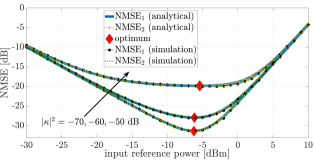
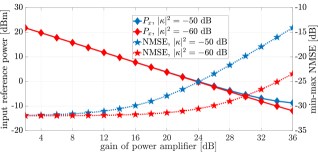
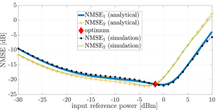
In this section, we simulate the impact of backward crosstalk and power amplifier non-linearity on the NMSE for a 2×2222\times 2 MIMO transmitter and on the SE of a 2×1212\times 1 MISO channel when using this 2×2222\times 2 transmitter.

First, we validate the Gaussian approximation derived in (22) by the solution of the non-linear equation system in (7) with (4) for a randomly generated Gaussian input 𝐱𝐱{\bf x} of length 10000. Then the corresponding 𝐮𝐮{\bf u} is obtained by using the “fsolve” function in MATLAB with the initial point 𝐐𝐱𝐐𝐱{\bf Q}{\bf x}. In this setup, the input power of two branches are the same (β=1𝛽1\beta=1) and the correlation coefficient is ξ=0𝜉0\xi=0. We consider a fully symmetric transmitter: κ1=κ2=κsubscript𝜅1subscript𝜅2𝜅\kappa_{1}=\kappa_{2}=\kappa, ρ1=ρ2=ρsubscript𝜌1subscript𝜌2𝜌\rho_{1}=\rho_{2}=\rho, and γ1=γ2=γsubscript𝛾1subscript𝛾2𝛾\gamma_{1}=\gamma_{2}=\gamma. The backward crosstalk parameter is selected as real and positive, and its power is 10log10(|κ|2)=5010subscript10superscript𝜅25010\log_{10}(|\kappa|^{2})=-50 dB. The power amplifier compression parameter is ρ=0.025𝜌0.025\rho=-0.025, and the thermal noise variance at the transmitter is σw2=10superscriptsubscript𝜎𝑤210\sigma_{w}^{2}=-10 dBm. The gain of power amplifier is 10log10(γ2)=3010subscript10superscript𝛾23010\log_{10}(\gamma^{2})=30 dB,333Note that the power of the leakage signal due to crosstalk is 10log10(|κ|2)+10log10(γ2)=2010subscript10superscript𝜅210subscript10superscript𝛾22010\log_{10}(|\kappa|^{2})+10\log_{10}(\gamma^{2})=-20 dB for this setup. where γ>0𝛾0\gamma>0 and γ2superscript𝛾2\gamma^{2} are the amplification and power gains, respectively. Since the transmitter is fully symmetric, both u1subscript𝑢1u_{1} and u2subscript𝑢2u_{2} have the same distribution and the cumulative distribution function (CDF) of the real and imaginary parts of them are shown in Fig. 2 for three values of input reference power: Px=20subscript𝑃𝑥20P_{x}=-20, Px=10subscript𝑃𝑥10P_{x}=-10, and Px=0subscript𝑃𝑥0P_{x}=0 dBm. As Fig. 2 shows, the approximation in (22) matches well with the exact solution of the non-linear system. Furthermore, the NMSE for the covariance of u1subscript𝑢1u_{1} and u2subscript𝑢2u_{2} between two sets of data is given as 3232-32 dB, 2222-22 dB, and 2929-29 dB, respectively for Px=20subscript𝑃𝑥20P_{x}=-20, Px=10subscript𝑃𝑥10P_{x}=-10, and Px=0subscript𝑃𝑥0P_{x}=0 dBm.

V-A NMSE Performance

We consider again the fully symmetric transmitter described above. Hence, the NMSE of the two branches are identical: NMSE1(Px)=NMSE2(Px)subscriptNMSE1subscript𝑃𝑥subscriptNMSE2subscript𝑃𝑥{\mbox{NMSE}}_{1}(P_{x})={\mbox{NMSE}}_{2}(P_{x}). Fig. 3 shows NMSE=NMSE1=NMSE2NMSEsubscriptNMSE1subscriptNMSE2{\mbox{NMSE}}={\mbox{NMSE}}_{1}={\mbox{NMSE}}_{2} versus the input reference power, Pxsubscript𝑃𝑥P_{x} for three levels of crosstalk: |κ|2=70superscript𝜅270|\kappa|^{2}=-70 dB, |κ|2=60superscript𝜅260|\kappa|^{2}=-60 dB, and |κ|2=50superscript𝜅250|\kappa|^{2}=-50 dB. Both the derived analytical results and simulation results obtained by averaging the Monte Carlo trials with the exact solution of the non-linear system are shown. The optimal solution of the min-max NMSE problem is shown by the red diamond. Since the NMSE for two branches is the same, the optimal Pxsubscript𝑃𝑥P_{x} is the minimizer of NMSE1(Px)=NMSE2(Px)subscriptNMSE1subscript𝑃𝑥subscriptNMSE2subscript𝑃𝑥{\mbox{NMSE}}_{1}(P_{x})={\mbox{NMSE}}_{2}(P_{x}). Although there are some slight deviations between the simulation and the analytical results obtained by the Gaussian approximation for 𝐮𝐮{\bf u} at some points, the closed-form results match very well with the simulation.

As seen from Fig. 3, as the crosstalk power decreases, the NMSE becomes more sensitive to the changes in input reference power, Pxsubscript𝑃𝑥P_{x}. For |κ|2=70superscript𝜅270|\kappa|^{2}=-70 dB, the optimum Pxsubscript𝑃𝑥P_{x} is around -6 dBm. When we decrease Pxsubscript𝑃𝑥P_{x} to -10 dBm or increase it to -2 dBm, the NMSE increases by around 2 dB. Moreover, the optimal Pxsubscript𝑃𝑥P_{x} also changes with the crosstalk level.
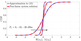
Refer to caption
Figure 2: The CDF of {u}subscript𝑢\Re\{u_{\ell}\} and {u}subscript𝑢\Im\{u_{\ell}\} for using the derived approximation and the solution of the non-linear system.
Refer to caption
Figure 3: NMSE versus input reference power, Pxsubscript𝑃𝑥P_{x} for a symmetric transmitter.
Refer to caption
Figure 4: Optimal input reference power, Pxsubscript𝑃𝑥P_{x} and NMSE versus power gain, γ2superscript𝛾2\gamma^{2}, for a symmetric transmitter.
Refer to caption
Figure 5: NMSE versus input reference power, Pxsubscript𝑃𝑥P_{x} for the asymmetric transmitter.

In Fig. 4, we plot the optimal input reference power that minimizes NMSE1=NMSE2subscriptNMSE1subscriptNMSE2{\mbox{NMSE}}_{1}={\mbox{NMSE}}_{2} and the corresponding NMSE by changing the power gain of amplifier, 10log10(γ2)10subscript10superscript𝛾210\log_{10}(\gamma^{2}) dB. We consider two different backward crosstalk parameters: |κ|2=50superscript𝜅250|\kappa|^{2}=-50 dB or |κ|2=60superscript𝜅260|\kappa|^{2}=-60 dB. For both cases, as the gain of power amplifier increases, the value of Pxsubscript𝑃𝑥P_{x} that minimizes the NMSE decreases. For relatively smaller values of γ2superscript𝛾2\gamma^{2}, optimal input reference power for both crosstalk levels are nearly the same. After some point, the gap between the input powers starts to become visible. Higher input power is needed at the optimal point when the crosstalk level increases. As expected, the corresponding optimal NMSE is higher for |κ|2=50superscript𝜅250|\kappa|^{2}=-50 dB where the gap increases with the power amplifier gain.

Next, we consider the performance of an asymmetric transmitter with different power levels and non-zero correlation between the two input signals. The amplitude ratio of the second input signal to the first one is taken as β=1.3𝛽1.3\beta=1.3. The correlation coefficient is ξ=0.7𝜉0.7\xi=0.7. The backward crosstalk parameters are 10log10(|κ1|2)=4810subscript10superscriptsubscript𝜅124810\log_{10}(|\kappa_{1}|^{2})=-48 dB and 10log10(|κ2|2)=5210subscript10superscriptsubscript𝜅225210\log_{10}(|\kappa_{2}|^{2})=-52 dB. The power amplifier compression parameters are ρ1=0.023subscript𝜌10.023\rho_{1}=-0.023, and ρ2=0.027subscript𝜌20.027\rho_{2}=-0.027. The gains of the power amplifiers are the same: 10log10(γ2)=3010subscript10superscript𝛾23010\log_{10}(\gamma^{2})=30 dB.

Fig. 5 shows NMSE1subscriptNMSE1{\mbox{NMSE}}_{1} and NMSE2subscriptNMSE2{\mbox{NMSE}}_{2} for the asymmetric transmitter versus the input reference power, Pxsubscript𝑃𝑥P_{x}. The optimal solution of the min-max NMSE problem for this setup is where NMSE1(Px)=NMSE2(Px)subscriptNMSE1subscript𝑃𝑥subscriptNMSE2subscript𝑃𝑥{\mbox{NMSE}}_{1}(P_{x})={\mbox{NMSE}}_{2}(P_{x}) which corresponds to Case 3 in Appendix B. Note that NMSE1subscriptNMSE1{\mbox{NMSE}}_{1} achieves its minimum at a clearly different point. When Pxsubscript𝑃𝑥P_{x} deviates from its optimal value, either NMSE1subscriptNMSE1{\mbox{NMSE}}_{1} or NMSE2subscriptNMSE2{\mbox{NMSE}}_{2} increases and max{NMSE1,NMSE2}subscriptNMSE1subscriptNMSE2\max\{{\mbox{NMSE}}_{1},{\mbox{NMSE}}_{2}\} changes substantially. In addition, the optimal Pxsubscript𝑃𝑥P_{x} for the exact simulation data is approximately the same with the analytical one. This shows that the derived analytical results model the effect of dirty MIMO transmitter properly.
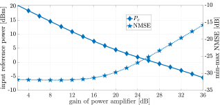
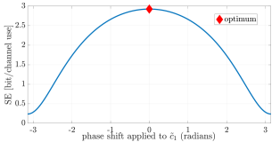
Refer to caption
Figure 6: Optimal input reference power, Pxsubscript𝑃𝑥P_{x} and NMSE versus γ2superscript𝛾2\gamma^{2} for the asymmetric transmitter.
Refer to caption
Figure 7: SE versus the phase shift applied to the optimal c~1subscript~𝑐1\tilde{c}_{1}.

We repeat the experiment in Fig. 4 but in the asymmetric transmitter case with 10log10(|κ1|2)=4810subscript10superscriptsubscript𝜅124810\log_{10}(|\kappa_{1}|^{2})=-48 dB and 10log10(|κ2|2)=5210subscript10superscriptsubscript𝜅225210\log_{10}(|\kappa_{2}|^{2})=-52 dB, and show the results in Fig. 6. We observe similar characteristics, except that the NMSE is around 5 dB greater for relatively small values of γ2superscript𝛾2\gamma^{2}.

V-B SE Performance

Now, we will consider the SE performance in the symmetric transmitter case described above. The channel coefficients are randomly and independently generated as h1,h2𝒩(0,1)similar-tosubscript1subscript2subscript𝒩01h_{1},h_{2}\sim\mathcal{N}_{\mathbb{C}}(0,1). The thermal noise variance at the receiver is taken as σn2superscriptsubscript𝜎𝑛2\sigma_{n}^{2}. Hence, channel gain over noise ratio is given by 1/σn21superscriptsubscript𝜎𝑛21/\sigma_{n}^{2}.

We first consider a single channel realization with σn2=1superscriptsubscript𝜎𝑛21\sigma_{n}^{2}=1 and verify the optimality of the proposed precoder in Theorem 2 that maximizes SE. Fig. 7 shows the SE when the first element of the optimal effective precoder, c~1subscript~𝑐1\tilde{c}_{1}, is phase shifted and all other parameters of the optimal precoder are kept constant. The zero phase shift corresponds to the proposed optimal precoder. As it can be seen from Fig. 7, when the phase of the optimal c~1subscript~𝑐1\tilde{c}_{1} is shifted, the SE can be reduced significantly compared to the optimal value. In Fig. 8, we are instead keeping the phases of the elements of the optimal effective precoder to be the same and scale c~1subscript~𝑐1\tilde{c}_{1} to see how the SE changes. We notice that the maximum SE is achieved when the scaling parameter is 1, which verifies the optimality of the proposed SE maximizing precoder. As the amplitude scaling increases above 1, the SE drops quickly towards zero. This is due to the decrease in the amplitude of the corresponding Bussgang gain and increased distortion level.
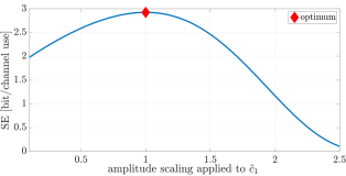
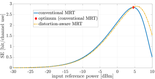
Refer to caption
Figure 8: SE versus the amplitude scaling applied to the optimal c~1subscript~𝑐1\tilde{c}_{1}.
Refer to caption
Figure 9: SE versus input reference power, Pxsubscript𝑃𝑥P_{x}, for conventional and distortion-aware MRT.

For the same single channel realization, Fig. 9 shows the SE versus input reference power, Pxsubscript𝑃𝑥P_{x}, for conventional and distortion-aware MRT. The proposed optimal solution for conventional MRT is shown by the red diamond and it obviously maximizes the SE. The SE curve for distortion-aware MRT is obtained by a line search over η𝜂\eta and using the relations in (107). We observe that the SE versus Pxsubscript𝑃𝑥P_{x} has a uni-modal characteristic. Furthermore, the gap between the SE curves for two precoders are very close for Px5subscript𝑃𝑥5P_{x}\leq 5 dBm. For higher values of Pxsubscript𝑃𝑥P_{x}, the distortion-aware MRT provides higher SE compared to the conventional MRT by exploiting the distortion characteristics. We note that although these two sub-optimal precoders do not utilize the full information related to the crosstalk distortion, the optimal Pxsubscript𝑃𝑥P_{x} is dependent on the all the hardware parameters. Hence, by neglecting crosstalk, the SE may deteriorate significantly. In the following experiments, we will find the optimal Pxsubscript𝑃𝑥P_{x} for the distortion-aware MRT by a line search over η𝜂\eta. Interestingly, the SE-maximizing input power is substantially higher (around 10 dB) than the NMSE-minimizing input power, which was shown in Fig. 3.

We now consider 1000 random channel realizations and plot the average SE for all the considered precoders: a) the optimal precoder that maximizes SE, b) distortion-aware MRT with optimized Pxsubscript𝑃𝑥P_{x}, c) conventional MRT with optimized Pxsubscript𝑃𝑥P_{x}. In Fig. 10, the SE performance of the three precoders is considered by changing channel gain over noise. Although there is a slight difference between the SE of the considered precoders, it is possible to attain the same SE with approximately 0.7 dB and 0.5 dB worse channel gain compared to the conventional MRT and the distortion-aware MRT, respectively. Hence, although the hardware distortion has clear impact on the SE, the same precoding still works fairly well.
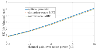
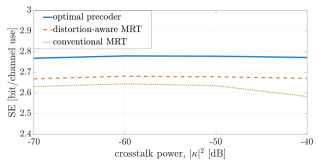
Refer to caption
Figure 10: Average SE versus channel gain over noise 1/σn21superscriptsubscript𝜎𝑛21/\sigma_{n}^{2}.
Refer to caption
Figure 11: Average SE versus crosstalk power, |κ|2superscript𝜅2|\kappa|^{2}.

In Fig. 11, we set the channel gain over noise to 0 dB and analyze the effect of the crosstalk parameter, κ𝜅\kappa, on the SE. The performance of the optimal precoder and the distortion-aware MRT is barely affected by the crosstalk change. This is due to the fact that they both exploit the structure of the matrix 𝐐𝐐{\bf Q} that is determined by the power amplifier gains and crosstalk parameters. The non-diagonal structure of this matrix yields that the optimal phase difference between the precoder weights is not equal to the phase difference between the channels of two antennas. In conventional MRT, the effect of 𝐐𝐐{\bf Q} is neglected and the phase deterioration results in a consistent drop in the SE with the increase of crosstalk strength after -60 dB although the input reference power is also optimized.

According to our observations, the optimal input reference power for maximum SE changes substantially with different channel realizations even if the channel variance is the same. This is typical for fading channels. Furthermore, it may significantly differ from the input reference power that minimizes the maximum NMSE of the two transmitter branches. One can often use a higher power for data transmission since the SE grows with Pxsubscript𝑃𝑥P_{x} as long as the numerator of the SNDR increases faster than the denominator.

VI Extension of M×M𝑀𝑀M\times M MIMO Transmitters

In this section, we will discuss how the analytical results derived in the previous sections can be extended to M×M𝑀𝑀M\times M MIMO transmitters. For such a transmitter with M𝑀M antennas, a feedback connection can be drawn as in Fig. 1 between two different antenna branches with crosstalk parameters κ,msubscript𝜅𝑚\kappa_{\ell,m}\in\mathbb{C}, where κ,msubscript𝜅𝑚\kappa_{\ell,m} is the scaling factor from the \ellth antenna branch to the m𝑚mth one. The input signal is 𝐱=(x1xM)T𝒩(𝟎,𝐂𝐱)𝐱superscriptsubscript𝑥1subscript𝑥𝑀𝑇similar-tosubscript𝒩0subscript𝐂𝐱{\bf x}=(x_{1}\ldots x_{M})^{T}\sim\mathcal{N}_{\mathbb{C}}\left({\bf 0},{\bf C_{x}}\right) where 𝐂𝐱M×Msubscript𝐂𝐱superscript𝑀𝑀{\bf C_{x}}\in\mathbb{C}^{M\times M} depends only one design parameter that is Px=𝔼[|x1|2]subscript𝑃𝑥𝔼delimited-[]superscriptsubscript𝑥12P_{x}=\mathbb{E}[|x_{1}|^{2}] as in (1). The output of the transmitter is given by 𝐲=𝐫+𝐰𝐲𝐫𝐰{\bf y}={\bf r}+{\bf w}, where the only difference compared to Section II is that all the vectors are M𝑀M-dimensional. The power amplifier outputs can be represented as in (4) with an M𝑀M-dimensional counterpart of the diagonal matrix 𝐆𝐆{\bf G} and the third-order distortion function 𝐟(𝐮)𝐟𝐮{\bf f}({\bf u}). All the equations in (5)–(9) are also valid for M×M𝑀𝑀M\times M transmitter with appropriately defined matrices. Note that the gain matrix 𝐋𝐋{\bf L} is diagonal with entries γsubscript𝛾\gamma_{\ell}, for =1,,M1𝑀\ell=1,\ldots,M and the feedback matrix 𝐊𝐊{\bf K} has zero diagonal elements with the (,m)𝑚\left(\ell,m\right)th element being γκm,subscript𝛾subscript𝜅𝑚\gamma_{\ell}\kappa_{m,\ell}, for m𝑚\ell\neq m. Using the same small-error approximations, a similar relationship can be obtained as in (22), where the elements of the matrix 𝐐M×M𝐐superscript𝑀𝑀{\bf Q}\in\mathbb{C}^{M\times M} all depend on the constant system parameters. Using this linear relation, the covariance matrix 𝐔𝐔{\bf U} becomes Px𝐓subscript𝑃𝑥𝐓P_{x}{\bf T} where the elements of the constant matrix 𝐓M×M𝐓superscript𝑀𝑀{\bf T}\in\mathbb{C}^{M\times M}, i.e., tmsubscript𝑡𝑚t_{\ell m} can easily be determined as in (27)–(29). Furthermore, the Bussgang matrix 𝐀𝐀{\bf A} is diagonal with elements a=1+2ρusubscript𝑎12subscript𝜌subscript𝑢a_{\ell}=1+2\rho_{\ell}u_{\ell\ell} when the power amplifier non-linearities affect each antenna signal separately [16, Sec. II.B].

Note that the simplified expressions for the fourth-order and the sixth-order matrices in Appendix A hold for any M𝑀M with proper dimensions. Using this fact and taking similar steps as in Section III, we can express the diagonal elements of the error covariance matrix 𝐄𝐄{\bf E} as the third-order polynomial functions of the reference input power, Pxsubscript𝑃𝑥P_{x} with the coefficient of Px3superscriptsubscript𝑃𝑥3P_{x}^{3} terms being positive. Hence, the NMSE for each transmitter branch becomes a convex function of Pxsubscript𝑃𝑥P_{x} as claimed by Lemma 1 and the min-max fair optimization problem in (68) is a convex programming problem. When M𝑀M is relatively large and the transmitter is asymmetric, checking all the candidate solutions in Theorem 1 is not efficient and a numerical solver should be utilized.

The optimal precoder that maximizes the SE may not be obtainable in a simple form for M>2𝑀2M>2 since the number of canditate solutions to be checked increases exponentially. However, for conventional MRT and distortion-aware MRT, the same steps in Section IV-B and Section IV-C can be followed to obtain the similar one-dimensional optimization problems with properly defined parameters.

VII Conclusions

In this paper, a non-ideal 2×2222\times 2 MIMO transmitter subject to backward crosstalk and power amplifier non-linearities has been analyzed using Bussgang theory for OFDM transmission. By utilizing the signal statistics, the feedback model for the backward crosstalk was reformulated as an approximately linear relation between the transmitter outputs and inputs. The NMSE compared to the ideal amplified signal at the transmitter output was derived in closed form. It was used to find the power back-off that minimizes the maximum NMSE of two branches. In general, the optimal value will not minimize both NMSEs, but find a suitable trade-off.

The SE of transmission to a single-antenna receiver has also been analyzed and a closed-form achievable SE was derived using the fact that the effective distortion noise in the Bussgang decomposition is uncorrelated with the desired communication signal. Three different precoders were considered. The first one maximizes the SE by exploiting full knowledge of the parameters in the backward crosstalk and power amplifier non-linearity models. One of the two sub-optimal precoders uses the optimal precoder structure for ideal hardware and the other one assumes partial knowledge about the backward crosstalk. We optimized the power back-off for maximum SE also for the sub-optimal solutions. Simulation results showed that the sub-optimal precoders achieve almost the same SE as the optimal precoder; thus, it is not of critical importance to estimate the hardware parameters in practice. However, when the strength of the crosstalk increases, the SE achieved by the sub-optimal precoder that assumes ideal hardware got worse compared to the others. Finally, we also noticed that the SE is often maximized when transmitting at a higher power than what is minimizing the NMSE.

Appendix A Derivation of the Elements of 𝐕𝐕{\bf V}

The elements of the matrix 𝐕𝐕{\bf V} in (51) depend on the matrices 𝐔¯¯𝐔\overline{\bf U} and 𝐔¯¯¯¯𝐔\overline{\overline{\bf U}}, which contain fourth- and sixth-order moments of the input signals. These matrices will be derived in this appendix, which finally leads to the simplified expression in (52).

Fourth-Order Moments 𝐔¯¯𝐔\overline{\bf U}

For the third-order nonlinearity 𝐟(𝐮)𝐟𝐮{\bf f}({\bf u}) in (4), the fourth-order moments in 𝐔¯=𝔼[𝐟(𝐮)𝐮H]¯𝐔𝔼delimited-[]𝐟𝐮superscript𝐮𝐻\overline{\bf U}=\mathbb{E}[{\bf f}({\bf u})\,{\bf u}^{H}] read

u¯subscript¯𝑢\displaystyle\overline{u}_{\ell\ell} \displaystyle\triangleq 𝔼[u|u|2u]=2u2,=1,2,formulae-sequence𝔼delimited-[]subscript𝑢superscriptsubscript𝑢2superscriptsubscript𝑢2superscriptsubscript𝑢212\displaystyle\mathbb{E}[u_{\ell}\,|u_{\ell}|^{2}\,u_{\ell}^{*}]=2\,u_{\ell\ell}^{2},\quad\ell=1,2, (108)
u¯ksubscript¯𝑢𝑘\displaystyle\overline{u}_{k\ell} \displaystyle\triangleq 𝔼[uk|uk|2u]=2ukkuk,k,formulae-sequence𝔼delimited-[]subscript𝑢𝑘superscriptsubscript𝑢𝑘2superscriptsubscript𝑢2subscript𝑢𝑘𝑘superscriptsubscript𝑢𝑘𝑘\displaystyle\mathbb{E}[u_{k}\,|u_{k}|^{2}\,u_{\ell}^{*}]=2\,u_{kk}\,u_{\ell k}^{*},\quad\ell\neq k, (109)

where 𝔼[uk|uk|2u]=2𝔼[ukuk]𝔼[uku]𝔼delimited-[]subscript𝑢𝑘superscriptsubscript𝑢𝑘2superscriptsubscript𝑢2𝔼delimited-[]subscript𝑢𝑘superscriptsubscript𝑢𝑘𝔼delimited-[]subscript𝑢𝑘superscriptsubscript𝑢\mathbb{E}[u_{k}\,|u_{k}|^{2}\,u_{\ell}^{*}]=2\,\mathbb{E}[u_{k}\,u_{k}^{*}]\,\mathbb{E}[u_{k}\,u_{\ell}^{*}] was used [24]. The higher-order moments matrix 𝐔¯¯𝐔\overline{\bf U} is now given by

𝐔¯=2(u1100u22)𝐁(u11u12u12u22)𝐔.¯𝐔2subscriptsubscript𝑢1100subscript𝑢22𝐁subscriptsubscript𝑢11subscript𝑢12superscriptsubscript𝑢12subscript𝑢22𝐔\overline{\bf U}=2\underbrace{\left(\begin{array}[]{cc}u_{11}&0\\ 0&u_{22}\end{array}\right)}_{\displaystyle{\bf B}}\,\underbrace{\left(\begin{array}[]{cc}u_{11}&u_{12}\\ u_{12}^{*}&u_{22}\end{array}\right)}_{\displaystyle{\bf U}}. (110)

Sixth-Order Moments 𝐔¯¯¯¯𝐔\overline{\overline{\bf U}}

For the third-order nonlinearity 𝐟(𝐮)𝐟𝐮{\bf f}({\bf u}) in (4), the components of 𝐔¯¯=𝔼[𝐟(𝐮)𝐟(𝐮)H]¯¯𝐔𝔼delimited-[]𝐟𝐮𝐟superscript𝐮𝐻\overline{\overline{\bf U}}=\mathbb{E}[{\bf f}({\bf u})\,{\bf f}({\bf u})^{H}] read

u¯¯subscript¯¯𝑢\displaystyle\overline{\overline{u}}_{\ell\ell} \displaystyle\triangleq 𝔼[u|u|2u|u|2]=6u3,=1,2,formulae-sequence𝔼delimited-[]subscript𝑢superscriptsubscript𝑢2superscriptsubscript𝑢superscriptsubscript𝑢26superscriptsubscript𝑢312\displaystyle\mathbb{E}[u_{\ell}\,|u_{\ell}|^{2}\,u_{\ell}^{*}\,|u_{\ell}|^{2}]=6\,u_{\ell\ell}^{3},\quad\ell=1,2, (111)
u¯¯12subscript¯¯𝑢12\displaystyle\overline{\overline{u}}_{12} \displaystyle\triangleq 𝔼[u1|u1|2u2|u2|2]=𝔼[(u1u2)2(u1u2)]𝔼delimited-[]subscript𝑢1superscriptsubscript𝑢12superscriptsubscript𝑢2superscriptsubscript𝑢22𝔼delimited-[]superscriptsubscript𝑢1superscriptsubscript𝑢22superscriptsubscript𝑢1superscriptsubscript𝑢2\displaystyle\mathbb{E}[u_{1}\,|u_{1}|^{2}\,u_{2}^{*}\,|u_{2}|^{2}]=\mathbb{E}[(u_{1}\,u_{2}^{*})^{2}\,(u_{1}\,u_{2}^{*})^{*}] (112)
=\displaystyle= 4u12u11u22+2u12|u12|2,4subscript𝑢12subscript𝑢11subscript𝑢222subscript𝑢12superscriptsubscript𝑢122\displaystyle 4u_{12}\,u_{11}\,u_{22}+2u_{12}\,|u_{12}|^{2},

where the following results was used [24]:

𝔼[(uuk)2(uuk)]𝔼delimited-[]superscriptsubscript𝑢superscriptsubscript𝑢𝑘2superscriptsubscript𝑢superscriptsubscript𝑢𝑘\displaystyle\mathbb{E}[(u_{\ell}\,u_{k}^{*})^{2}(u_{\ell}\,u_{k}^{*})^{*}]
=4𝔼[uuk]𝔼[uu]𝔼[ukuk]+2𝔼[uuk]2𝔼[uuk].absent4𝔼delimited-[]subscript𝑢superscriptsubscript𝑢𝑘𝔼delimited-[]subscript𝑢superscriptsubscript𝑢𝔼delimited-[]subscript𝑢𝑘superscriptsubscript𝑢𝑘2𝔼superscriptdelimited-[]subscript𝑢superscriptsubscript𝑢𝑘2𝔼delimited-[]superscriptsubscript𝑢subscript𝑢𝑘\displaystyle=4\mathbb{E}[u_{\ell}\,u_{k}^{*}]\,\mathbb{E}[u_{\ell}\,u_{\ell}^{*}]\,\mathbb{E}[u_{k}\,u_{k}^{*}]+2\mathbb{E}[u_{\ell}\,u_{k}^{*}]^{2}\,\mathbb{E}[u_{\ell}^{*}\,u_{k}]. (113)

The matrix 𝐔¯¯¯¯𝐔\overline{\overline{\bf U}} can now be divided into two terms as

𝐔¯¯¯¯𝐔\displaystyle\overline{\overline{\bf U}} =\displaystyle= 4(u113u12u11u22u12u11u22u223)4superscriptsubscript𝑢113subscript𝑢12subscript𝑢11subscript𝑢22superscriptsubscript𝑢12subscript𝑢11subscript𝑢22superscriptsubscript𝑢223\displaystyle 4\!\left(\!\!\!\begin{array}[]{cc}u_{11}^{3}&\!\!\!\!\!\!u_{12}\,u_{11}\,u_{22}\\ u_{12}^{*}\,u_{11}\,u_{22}&u_{22}^{3}\end{array}\!\!\!\right) (119)
+2(u113u12|u12|2u12|u12|2u223).2superscriptsubscript𝑢113subscript𝑢12superscriptsubscript𝑢122superscriptsubscript𝑢12superscriptsubscript𝑢122superscriptsubscript𝑢223\displaystyle\!+\!2\!\left(\!\!\!\begin{array}[]{cc}u_{11}^{3}&\!\!\!\!\!\!u_{12}\,|u_{12}|^{2}\\ u_{12}^{*}\,|u_{12}|^{2}&u_{22}^{3}\end{array}\!\!\!\right).

The result (119) can be expressed in 𝐁𝐁{\bf B} and 𝐔𝐔{\bf U} given in (110) as

𝐔¯¯=4𝐁𝐔𝐁+2𝐂,¯¯𝐔4𝐁𝐔𝐁2𝐂\overline{\overline{\bf U}}=4{\bf B}\,{\bf U}\,{\bf B}+2{\bf C}, (120)

where the matrix 𝐂𝐂{\bf C} was introduced as

𝐂=(u113u12|u12|2u12|u12|2u223).𝐂superscriptsubscript𝑢113subscript𝑢12superscriptsubscript𝑢122superscriptsubscript𝑢12superscriptsubscript𝑢122superscriptsubscript𝑢223\displaystyle{\bf C}=\left(\begin{array}[]{cc}u_{11}^{3}&u_{12}\,|u_{12}|^{2}\\ u_{12}^{*}\,|u_{12}|^{2}&u_{22}^{3}\end{array}\right). (123)

Final simplified expression

It follows directly from (110) that

𝐔¯𝐔1=2𝐁.¯𝐔superscript𝐔12𝐁\overline{\bf U}\,{\bf U}^{-1}=2{\bf B}. (124)

Furthermore, the matrix product 𝐔¯𝐔1𝐔¯H¯𝐔superscript𝐔1superscript¯𝐔𝐻\overline{\bf U}\,{\bf U}^{-1}\,\overline{\bf U}^{H} is required to evaluate the properties of the distortion noise. Combining (124) with (110) gives

𝐔¯𝐔1𝐔¯H=4𝐁𝐔𝐁,¯𝐔superscript𝐔1superscript¯𝐔𝐻4𝐁𝐔𝐁\overline{\bf U}\,{\bf U}^{-1}\,\overline{\bf U}^{H}=4{\bf B}\,{\bf U}\,{\bf B}, (125)

where the result follows from the fact that 𝐁=𝐁H𝐁superscript𝐁𝐻{\bf B}={\bf B}^{H}, and that 𝐔=𝐔H𝐔superscript𝐔𝐻{\bf U}={\bf U}^{H}. From (120) and (125) it now directly follows that

𝐔¯¯𝐔¯𝐔1𝐔¯H=2𝐂,¯¯𝐔¯𝐔superscript𝐔1superscript¯𝐔𝐻2𝐂\displaystyle\overline{\overline{\bf U}}-\overline{\bf U}\,{\bf U}^{-1}\,\overline{\bf U}^{H}=2{\bf C}, (126)

where 𝐂𝐂{\bf C} is given in (123). This leads to simplified expression in (52).

Appendix B Proof of Theorem 1

There are three cases to be evaluated to achieve the optimal solution to the problem (68) since we minimize the maximum of two convex functions. The optimal input reference power, Pxsubscript𝑃𝑥P_{x} is either the minimizer of NMSE1subscriptNMSE1{\mbox{NMSE}}_{1} or NMSE2subscriptNMSE2{\mbox{NMSE}}_{2}, or the one at which the NMSE1=NMSE2subscriptNMSE1subscriptNMSE2{\mbox{NMSE}}_{1}={\mbox{NMSE}}_{2} are equal. These three candidate solutions are given as follows:

Case 1: The unique minimizer of NMSE1(Px)subscriptNMSE1subscript𝑃𝑥{\mbox{NMSE}}_{1}(P_{x}), which is denoted Px(1)superscriptsubscript𝑃𝑥1P_{x}^{(1)}, is a solution to the equation

12ρ12t113γ12Px+4γ2t11ρ1(γ2β2|κ2|2+β{κ2ξ})=σw2γ12Px2,12superscriptsubscript𝜌12superscriptsubscript𝑡113superscriptsubscript𝛾12subscript𝑃𝑥4subscript𝛾2subscript𝑡11subscript𝜌1subscript𝛾2superscript𝛽2superscriptsubscript𝜅22𝛽subscript𝜅2superscript𝜉superscriptsubscript𝜎𝑤2superscriptsubscript𝛾12superscriptsubscript𝑃𝑥2\displaystyle\frac{12\rho_{1}^{2}\,t_{11}^{3}}{\gamma_{1}^{2}}\,P_{x}+4\gamma_{2}t_{11}\rho_{1}\left(\gamma_{2}\beta^{2}\left|\kappa_{2}\right|^{2}+\beta\Re\left\{\kappa_{2}\xi^{*}\right\}\right)=\frac{\sigma_{w}^{2}}{\gamma_{1}^{2}\,P_{x}^{2}}, (127)

which is obtained by taking the first derivative of NMSE1(Px)subscriptNMSE1subscript𝑃𝑥{\mbox{NMSE}}_{1}(P_{x}) with respect to Pxsubscript𝑃𝑥P_{x} and equating it to zero. Since NMSE1subscriptNMSE1{\mbox{NMSE}}_{1} is a convex function of Pxsubscript𝑃𝑥P_{x}, the candidate solution for this case is the only positive root of the third-order polynomial of Pxsubscript𝑃𝑥P_{x} in (70).

Case 2: Similarly, we find the unique minimizer of NMSE2(Px)subscriptNMSE2subscript𝑃𝑥{\mbox{NMSE}}_{2}(P_{x}), which is denoted Px(2)superscriptsubscript𝑃𝑥2P_{x}^{(2)}, as a solution to the equation

12ρ22t223γ22β2Px+4γ1t22ρ2β2(γ1|κ1|2+β{κ1ξ})=σw2γ22β2Px2,12superscriptsubscript𝜌22superscriptsubscript𝑡223superscriptsubscript𝛾22superscript𝛽2subscript𝑃𝑥4subscript𝛾1subscript𝑡22subscript𝜌2superscript𝛽2subscript𝛾1superscriptsubscript𝜅12𝛽subscript𝜅1𝜉superscriptsubscript𝜎𝑤2superscriptsubscript𝛾22superscript𝛽2superscriptsubscript𝑃𝑥2\displaystyle\frac{12\rho_{2}^{2}\,t_{22}^{3}}{\gamma_{2}^{2}\beta^{2}}\,P_{x}+\frac{4\gamma_{1}t_{22}\rho_{2}}{\beta^{2}}\left(\gamma_{1}\left|\kappa_{1}\right|^{2}+\beta\Re\left\{\kappa_{1}\xi\right\}\right)=\frac{\sigma_{w}^{2}}{\gamma_{2}^{2}\,\beta^{2}P_{x}^{2}}, (128)

which is obtained by equating the first derivative of NMSE2(Px)subscriptNMSE2subscript𝑃𝑥{\mbox{NMSE}}_{2}(P_{x}) to zero. There is a unique positive root of the third-order polynomial of Pxsubscript𝑃𝑥P_{x} in (71).

Case 3: In this case, we take the candidate solution which satisfies NMSE1(Px)=NMSE2(Px)subscriptNMSE1subscript𝑃𝑥subscriptNMSE2subscript𝑃𝑥{\mbox{NMSE}}_{1}(P_{x})={\mbox{NMSE}}_{2}(P_{x}). These are the positive roots of the third-order polynomial in (72). Let Px(3)superscriptsubscript𝑃𝑥3P_{x}^{(3)} denote the positive root of (72) which makes NMSE1=NMSE2subscriptNMSE1subscriptNMSE2{\mbox{NMSE}}_{1}={\mbox{NMSE}}_{2} the smallest assuming there exists at least one positive root of (72). If all the roots are non-positive, then we can consider only Case 1 and 2.

Considering all the three cases, the optimal input reference signal power, Pxsubscript𝑃𝑥P_{x}, for the problem (68) is given by the element of the set 𝒮={Px(1),Px(2),Px(3)}𝒮superscriptsubscript𝑃𝑥1superscriptsubscript𝑃𝑥2superscriptsubscript𝑃𝑥3\mathcal{S}=\Big{\{}P_{x}^{(1)},P_{x}^{(2)},P_{x}^{(3)}\Big{\}} that minimizes the objective function max{NMSE1(Px),NMSE2(Px)}subscriptNMSE1subscript𝑃𝑥subscriptNMSE2subscript𝑃𝑥\max\big{\{}{\mbox{NMSE}}_{1}(P_{x}),{\mbox{NMSE}}_{2}(P_{x})\big{\}}.

Appendix C Proof of Theorem 2

In order to simplify the optimization in (93), we express the optimization variables c~1subscript~𝑐1\tilde{c}_{1} and c~2subscript~𝑐2\tilde{c}_{2} in terms of their amplitudes and phase components as follows:

c~1=ϱ1χ1,c~2=ϱ2χ2,ϱ1,ϱ2,χ1,χ2,formulae-sequencesubscript~𝑐1subscriptitalic-ϱ1subscript𝜒1formulae-sequencesubscript~𝑐2subscriptitalic-ϱ2subscript𝜒2subscriptitalic-ϱ1formulae-sequencesubscriptitalic-ϱ2subscript𝜒1subscript𝜒2\displaystyle\tilde{c}_{1}=\varrho_{1}\chi_{1},\ \ \tilde{c}_{2}=\varrho_{2}\chi_{2},\ \ \varrho_{1},\ \varrho_{2}\in\mathbb{R},\ \ \chi_{1},\ \chi_{2}\in\mathbb{C}, (129)
ϱ10,ϱ20,|χ1|2=1,|χ2|2=1.formulae-sequencesubscriptitalic-ϱ10formulae-sequencesubscriptitalic-ϱ20formulae-sequencesuperscriptsubscript𝜒121superscriptsubscript𝜒221\displaystyle\varrho_{1}\geq 0,\ \ \varrho_{2}\geq 0,\ \ |\chi_{1}|^{2}=1,\ \ |\chi_{2}|^{2}=1. (130)

By neglecting the constant 2 in the numerator of (93), we can cast the problem in terms of the amplitude and phase shift variables in (129):

maximizeϱ1,ϱ2,χ1,χ2|(h1ϱ1+h~1ϱ13)χ1+(h2ϱ2+h~2ϱ23)χ2|2|h~1ϱ13χ1+h~2ϱ23χ2|2+σ2subscriptitalic-ϱ1subscriptitalic-ϱ2subscript𝜒1subscript𝜒2maximizesuperscriptsubscript1subscriptitalic-ϱ1subscript~1superscriptsubscriptitalic-ϱ13subscript𝜒1subscript2subscriptitalic-ϱ2subscript~2superscriptsubscriptitalic-ϱ23subscript𝜒22superscriptsubscript~1superscriptsubscriptitalic-ϱ13subscript𝜒1subscript~2superscriptsubscriptitalic-ϱ23subscript𝜒22superscript𝜎2\displaystyle\underset{\varrho_{1},\ \varrho_{2},\,\chi_{1},\ \chi_{2}}{\text{maximize}}\ \ \ \frac{\left|\left(h_{1}\varrho_{1}+\tilde{h}_{1}\varrho_{1}^{3}\right)\chi_{1}+\left(h_{2}\varrho_{2}+\tilde{h}_{2}\varrho_{2}^{3}\right)\chi_{2}\right|^{2}}{\left|\tilde{h}_{1}\varrho_{1}^{3}\chi_{1}+\tilde{h}_{2}\varrho_{2}^{3}\chi_{2}\right|^{2}+\sigma^{2}} (131)
subject toϱ10,ϱ20,|χ1|2=1,|χ2|2=1.formulae-sequencesubject tosubscriptitalic-ϱ10formulae-sequencesubscriptitalic-ϱ20formulae-sequencesuperscriptsubscript𝜒121superscriptsubscript𝜒221\displaystyle\text{subject to}\ \ \varrho_{1}\geq 0,\ \ \varrho_{2}\geq 0,\ \ |\chi_{1}|^{2}=1,\ \ |\chi_{2}|^{2}=1. (132)

We observe that the objective function does not change if a common phase rotation is applied to χ1subscript𝜒1\chi_{1} and χ2subscript𝜒2\chi_{2}. This means that if {χ1,χ2}superscriptsubscript𝜒1superscriptsubscript𝜒2\left\{\chi_{1}^{\star},\ \chi_{2}^{\star}\right\} are the optimal phase shifts, then {χ1ejθ,χ2ejθ}superscriptsubscript𝜒1superscript𝑒𝑗𝜃superscriptsubscript𝜒2superscript𝑒𝑗𝜃\left\{\chi_{1}^{\star}e^{j\theta},\ \chi_{2}^{\star}e^{j\theta}\right\} result in the same optimal objective for any θ[0,2π)𝜃02𝜋\theta\in[0,2\pi). Using this observation, we can simply take χ2=1subscript𝜒21\chi_{2}=1 and consider the optimization problem in terms of ϱ1,ϱ2subscriptitalic-ϱ1subscriptitalic-ϱ2\varrho_{1},\ \varrho_{2}, and χ1subscript𝜒1\chi_{1}. For this reduced-size problem, we obtain the necessary optimality condition for χ1subscript𝜒1\chi_{1} as follows:

DEN(h1ϱ1+h~1ϱ13)(h2ϱ2+h~2ϱ23)DENsuperscriptsubscript1subscriptitalic-ϱ1subscript~1superscriptsubscriptitalic-ϱ13subscript2subscriptitalic-ϱ2subscript~2superscriptsubscriptitalic-ϱ23\displaystyle\text{DEN}\left(h_{1}\varrho_{1}+\tilde{h}_{1}\varrho_{1}^{3}\right)^{*}\left(h_{2}\varrho_{2}+\tilde{h}_{2}\varrho_{2}^{3}\right)
NUM(h~1ϱ13)h~2ϱ23=1χ1,NUMsuperscriptsubscript~1superscriptsubscriptitalic-ϱ13subscript~2superscriptsubscriptitalic-ϱ23subscript1subscript𝜒1\displaystyle-\text{NUM}\left(\tilde{h}_{1}\varrho_{1}^{3}\right)^{*}\tilde{h}_{2}\varrho_{2}^{3}=\mathcal{L}_{1}\chi_{1}, (133)

where DEN and NUM denote the denominator and numerator of the objective function in (131). Note that they are both real and non-negative. 1subscript1\mathcal{L}_{1} is the real scaled Lagrange multiplier corresponding to the equality |χ1|2=1superscriptsubscript𝜒121|\chi_{1}|^{2}=1. Now, we have

χ1=ej(DEN1(h1ϱ1+h~1ϱ13)(h2ϱ2+h~2ϱ23)NUM1(h~1ϱ13)h~2ϱ23).subscript𝜒1superscript𝑒𝑗DENsubscript1superscriptsubscript1subscriptitalic-ϱ1subscript~1superscriptsubscriptitalic-ϱ13subscript2subscriptitalic-ϱ2subscript~2superscriptsubscriptitalic-ϱ23NUMsubscript1superscriptsubscript~1superscriptsubscriptitalic-ϱ13subscript~2superscriptsubscriptitalic-ϱ23\displaystyle\chi_{1}=e^{j\angle\left(\frac{\text{DEN}}{\mathcal{L}_{1}}\left(h_{1}\varrho_{1}+\tilde{h}_{1}\varrho_{1}^{3}\right)^{*}\left(h_{2}\varrho_{2}+\tilde{h}_{2}\varrho_{2}^{3}\right)-\frac{\text{NUM}}{\mathcal{L}_{1}}\left(\tilde{h}_{1}\varrho_{1}^{3}\right)^{*}\tilde{h}_{2}\varrho_{2}^{3}\right)}. (134)

Using the definitions of h~1subscript~1\tilde{h}_{1} and h~2subscript~2\tilde{h}_{2} in (94) and noting that ρ1<0subscript𝜌10\rho_{1}<0 and ρ2<0subscript𝜌20\rho_{2}<0 are real scalars, we see that the angle of (h1ϱ1+h~1ϱ13)subscript1subscriptitalic-ϱ1subscript~1superscriptsubscriptitalic-ϱ13\left(h_{1}\varrho_{1}+\tilde{h}_{1}\varrho_{1}^{3}\right) is either h1subscript1\angle{h_{1}} or h1+πsubscript1𝜋\angle{h_{1}}+\pi. Similar reasoning applies for (h2ϱ2+h~2ϱ23)subscript2subscriptitalic-ϱ2subscript~2superscriptsubscriptitalic-ϱ23\left(h_{2}\varrho_{2}+\tilde{h}_{2}\varrho_{2}^{3}\right). Hence, considering the two possible sign values for 1subscript1\mathcal{L}_{1}, we have two possibilities for the angle of χ1subscript𝜒1\chi_{1} which are

χ1=h1h2,orχ1=h1h2+π.formulae-sequencesubscript𝜒1superscriptsubscript1subscript2orsubscript𝜒1superscriptsubscript1subscript2𝜋\displaystyle\angle{\chi_{1}}=\angle{h_{1}^{*}h_{2}},\ \ \text{or}\ \ \angle{\chi_{1}}=\angle{h_{1}^{*}h_{2}}+\pi. (135)

Now, our aim is to find the optimal set of {ϱ1,ϱ2}subscriptitalic-ϱ1subscriptitalic-ϱ2\{\varrho_{1},\varrho_{2}\} for these two possibilities. Let us explore two cases one by one.

Case 1: In this case, we take the candidate solution χ1=ejh1h2subscript𝜒1superscript𝑒𝑗superscriptsubscript1subscript2\chi_{1}=e^{j\angle{h_{1}^{*}h_{2}}} together with χ2=1subscript𝜒21\chi_{2}=1. The maximization problem in (131)-(132) can be expressed in terms of ϱ1subscriptitalic-ϱ1\varrho_{1} and ϱ2subscriptitalic-ϱ2\varrho_{2} as follows:

maximizeϱ1,ϱ2(|h1|(ϱ1+2ρ1ϱ13)+|h2|(ϱ2+2ρ2ϱ23))2(|h~1|ϱ13+|h~2|ϱ23)2+σ2subscriptitalic-ϱ1subscriptitalic-ϱ2maximizesuperscriptsubscript1subscriptitalic-ϱ12subscript𝜌1superscriptsubscriptitalic-ϱ13subscript2subscriptitalic-ϱ22subscript𝜌2superscriptsubscriptitalic-ϱ232superscriptsubscript~1superscriptsubscriptitalic-ϱ13subscript~2superscriptsubscriptitalic-ϱ232superscript𝜎2\displaystyle\underset{\varrho_{1},\varrho_{2}}{\text{maximize}}\ \ \ \frac{\left(\left|h_{1}\right|\left(\varrho_{1}+2\rho_{1}\varrho_{1}^{3}\right)+\left|h_{2}\right|\left(\varrho_{2}+2\rho_{2}\varrho_{2}^{3}\right)\right)^{2}}{\left(\left|\tilde{h}_{1}\right|\varrho_{1}^{3}+\left|\tilde{h}_{2}\right|\varrho_{2}^{3}\right)^{2}+\sigma^{2}} (136)
subject toϱ10,ϱ20.formulae-sequencesubject tosubscriptitalic-ϱ10subscriptitalic-ϱ20\displaystyle\text{subject to}\ \ \varrho_{1}\geq 0,\ \ \varrho_{2}\geq 0. (137)

By KKT conditions for the problem in (136)-(137), there are four subcases according to complementary slackness conditions and the Lagrange multipliers for (137). These cases are as follows:

Case 1-A: The first case is ϱ1=ϱ2=0subscriptitalic-ϱ1subscriptitalic-ϱ20\varrho_{1}=\varrho_{2}=0 where both variables are at the boundary. This case results in zero SNDR and is obviously not the optimal solution.

Case 1-B: In this case, we take ϱ1=0subscriptitalic-ϱ10\varrho_{1}=0 and do not put any constraint on ϱ2subscriptitalic-ϱ2\varrho_{2}. After inserting ϱ1=0subscriptitalic-ϱ10\varrho_{1}=0 into the objective function and by equating the derivative of it with respect to ϱ2subscriptitalic-ϱ2\varrho_{2} to zero, we obtain

2ϱ2(2ρ2ϱ22+1)(2|h~2|2ϱ266ρ2σ2ϱ22σ2)(|h~2|2ϱ26+σ2)2=0,2subscriptitalic-ϱ22subscript𝜌2superscriptsubscriptitalic-ϱ2212superscriptsubscript~22superscriptsubscriptitalic-ϱ266subscript𝜌2superscript𝜎2superscriptsubscriptitalic-ϱ22superscript𝜎2superscriptsuperscriptsubscript~22superscriptsubscriptitalic-ϱ26superscript𝜎220\displaystyle-\frac{2\varrho_{2}\left(2\rho_{2}\varrho_{2}^{2}+1\right)\left(2\left|\tilde{h}_{2}\right|^{2}\varrho_{2}^{6}-6\rho_{2}\sigma^{2}\varrho_{2}^{2}-\sigma^{2}\right)}{\left(\left|\tilde{h}_{2}\right|^{2}\varrho_{2}^{6}+\sigma^{2}\right)^{2}}=0, (138)

where we obtain the critical points ϱ2(1-B-1)=12ρ2superscriptsubscriptitalic-ϱ21-B-112subscript𝜌2\varrho_{2}^{(\text{1-B-1})}=\sqrt{\frac{1}{-2\rho_{2}}} and the only positive root, ϱ2(1-B-2)superscriptsubscriptitalic-ϱ21-B-2\varrho_{2}^{(\text{1-B-2})}, of the polynomial in (97). We note the solution sets {0,ϱ2(1-B-1)}0superscriptsubscriptitalic-ϱ21-B-1\{0,\varrho_{2}^{(\text{1-B-1})}\} and {0,ϱ2(1-B-2)}0superscriptsubscriptitalic-ϱ21-B-2\{0,\varrho_{2}^{(\text{1-B-2})}\} as candidate optimum.

Case 1-C: This case is similar to Case 1-B, by the symmetric structure of the objective, i.e., now we take ϱ2=0subscriptitalic-ϱ20\varrho_{2}=0 and do not put any constraint on ϱ1subscriptitalic-ϱ1\varrho_{1}. After inserting ϱ2=0subscriptitalic-ϱ20\varrho_{2}=0 into the objective function and by equating the derivative of it with respect to ϱ1subscriptitalic-ϱ1\varrho_{1} to zero, we obtain the critical points as ϱ1(1-C-1)=12ρ1superscriptsubscriptitalic-ϱ11-C-112subscript𝜌1\varrho_{1}^{(\text{1-C-1})}=\sqrt{\frac{1}{-2\rho_{1}}} and the only positive root, ϱ1(1-C-2)superscriptsubscriptitalic-ϱ11-C-2\varrho_{1}^{(\text{1-C-2})}, of the polynomial in (98). We note the solution sets {ϱ1(1-C-1),0}superscriptsubscriptitalic-ϱ11-C-10\{\varrho_{1}^{(\text{1-C-1})},0\} and {ϱ1(1-C-2),0}superscriptsubscriptitalic-ϱ11-C-20\{\varrho_{1}^{(\text{1-C-2})},0\} as candidate optimum.

Case 1-D: In this case, we do not put any constraint on ϱ1subscriptitalic-ϱ1\varrho_{1} and ϱ2subscriptitalic-ϱ2\varrho_{2} and equate the Lagrange multipliers corresponding to the inequality constraints to zero. Then, by equating the derivatives of the objective function with respect to ϱ1subscriptitalic-ϱ1\varrho_{1} and ϱ2subscriptitalic-ϱ2\varrho_{2} to zero, we obtain the necessary optimality conditions. However, interpreting the resultant equations is hard. Instead, we consider an equivalent optimization problem:

maximizeϱ1,ϱ2,ϱ~1,ϱ~2(|h1|ϱ1|h~1|ϱ~1+|h2|ϱ2|h~2|ϱ~2)2(|h~1|ϱ~1+|h~2|ϱ~2)2+σ2subscriptitalic-ϱ1subscriptitalic-ϱ2subscript~italic-ϱ1subscript~italic-ϱ2maximizesuperscriptsubscript1subscriptitalic-ϱ1subscript~1subscript~italic-ϱ1subscript2subscriptitalic-ϱ2subscript~2subscript~italic-ϱ22superscriptsubscript~1subscript~italic-ϱ1subscript~2subscript~italic-ϱ22superscript𝜎2\displaystyle\underset{\varrho_{1},\ \varrho_{2},\ \tilde{\varrho}_{1},\ \tilde{\varrho}_{2}}{\text{maximize}}\ \ \ \frac{\left(\left|h_{1}\right|\varrho_{1}-\left|\tilde{h}_{1}\right|\tilde{\varrho}_{1}+\left|h_{2}\right|\varrho_{2}-\left|\tilde{h}_{2}\right|\tilde{\varrho}_{2}\right)^{2}}{\left(\left|\tilde{h}_{1}\right|\tilde{\varrho}_{1}+\left|\tilde{h}_{2}\right|\tilde{\varrho}_{2}\right)^{2}+\sigma^{2}} (139)
subject toϱ~1=ϱ13,ϱ~2=ϱ23.formulae-sequencesubject tosubscript~italic-ϱ1superscriptsubscriptitalic-ϱ13subscript~italic-ϱ2superscriptsubscriptitalic-ϱ23\displaystyle\text{subject to}\ \ \tilde{\varrho}_{1}=\varrho_{1}^{3},\ \ \tilde{\varrho}_{2}=\varrho_{2}^{3}. (140)

Note that we have included additional auxiliary variables, ϱ~1=ϱ13subscript~italic-ϱ1superscriptsubscriptitalic-ϱ13\tilde{\varrho}_{1}=\varrho_{1}^{3} and ϱ~2=ϱ23subscript~italic-ϱ2superscriptsubscriptitalic-ϱ23\tilde{\varrho}_{2}=\varrho_{2}^{3} in order to simplify the KKT conditions and omitted the non-negativity constraints for ϱ1subscriptitalic-ϱ1\varrho_{1} and ϱ2subscriptitalic-ϱ2\varrho_{2} since we assume in this case (Case 1-D), the Lagrange multipliers corresponding to these constraints are zero. However, we should select only the non-negative solutions of the problem (139)-(140) to be a candidate for the original problem. KKT conditions for the above problem are given as follows:

2|h|NUMDEN=3ϱ2,=1,2,formulae-sequence2subscriptNUMDEN3subscriptsuperscriptsubscriptitalic-ϱ212\displaystyle\frac{2\left|h_{\ell}\right|\text{NUM}}{\text{DEN}}=3\mathcal{L}_{\ell}\varrho_{\ell}^{2},\ \ \ \ell=1,2, (141)
2|h~|(NUMDEN+NUM2(|h~1|ϱ~1+|h~2|ϱ~2)DEN2)=,2subscript~NUMDENsuperscriptNUM2subscript~1subscript~italic-ϱ1subscript~2subscript~italic-ϱ2superscriptDEN2subscript\displaystyle-2\left|\tilde{h}_{\ell}\right|\left(\frac{\text{NUM}}{\text{DEN}}+\frac{\text{NUM}^{2}\left(\left|\tilde{h}_{1}\right|\tilde{\varrho}_{1}+\left|\tilde{h}_{2}\right|\tilde{\varrho}_{2}\right)}{\text{DEN}^{2}}\right)=-\mathcal{L}_{\ell},
=1,2,12\displaystyle\ell=1,2, (142)

where 1subscript1\mathcal{L}_{1} and 2subscript2\mathcal{L}_{2} are the Lagrange multipliers corresponding to the equalities in (140). NUM and DEN denote the term whose square is taken in the numerator and the denominator term of the objective function in (139), respectively, for ease of notation. By dividing both sides of (142) for =11\ell=1 and =22\ell=2, we obtain 1/2=|h~1|/|h~2|subscript1subscript2subscript~1subscript~2\mathcal{L}_{1}/\mathcal{L}_{2}=\left|\tilde{h}_{1}\right|/\left|\tilde{h}_{2}\right|. Using this relation in (141), we have

ϱ2=|ρ1||ρ2|ϱ1.subscriptitalic-ϱ2subscript𝜌1subscript𝜌2subscriptitalic-ϱ1\displaystyle\varrho_{2}=\sqrt{\frac{\left|\rho_{1}\right|}{\left|\rho_{2}\right|}}\varrho_{1}. (143)

If we insert ϱ2subscriptitalic-ϱ2\varrho_{2} in (143) into the original objective function, we obtain a similar problem as in Case 1-C and the critical points are ϱ1(1-C-1)=12ρ1superscriptsubscriptitalic-ϱ11-C-112subscript𝜌1\varrho_{1}^{(\text{1-C-1})}=\sqrt{\frac{1}{-2\rho_{1}}} and the only positive root, ϱ1(1-D)superscriptsubscriptitalic-ϱ11-D\varrho_{1}^{(\text{1-D})}, of the polynomial in (99). We note the solution sets {ϱ1(1-C-1),|ρ1||ρ2|ϱ1(1-C-1)}superscriptsubscriptitalic-ϱ11-C-1subscript𝜌1subscript𝜌2superscriptsubscriptitalic-ϱ11-C-1\{\varrho_{1}^{(\text{1-C-1})},\sqrt{\frac{\left|\rho_{1}\right|}{\left|\rho_{2}\right|}}\varrho_{1}^{(\text{1-C-1})}\} and {ϱ1(1-D),|ρ1||ρ2|ϱ1(1-D)}superscriptsubscriptitalic-ϱ11-Dsubscript𝜌1subscript𝜌2superscriptsubscriptitalic-ϱ11-D\{\varrho_{1}^{(\text{1-D})},\sqrt{\frac{\left|\rho_{1}\right|}{\left|\rho_{2}\right|}}\varrho_{1}^{(\text{1-D})}\} as candidate optimum.

Case 2: In this case, we take the other candidate solution χ1=ejh1h2+jπsubscript𝜒1superscript𝑒𝑗superscriptsubscript1subscript2𝑗𝜋\chi_{1}=e^{j\angle{h_{1}^{*}h_{2}}+j\pi} in (135) together with χ2=1subscript𝜒21\chi_{2}=1. In this case, the SNDR maximization problem in (131)-(132) can be expressed in terms of variables ϱ1subscriptitalic-ϱ1\varrho_{1} and ϱ2subscriptitalic-ϱ2\varrho_{2} as follows:

maximizeϱ1,ϱ2(|h1|(ϱ1+2ρ1ϱ13)|h2|(ϱ2+2ρ2ϱ23))2(|h~1|ϱ13|h~2|ϱ23)2+σ2subscriptitalic-ϱ1subscriptitalic-ϱ2maximizesuperscriptsubscript1subscriptitalic-ϱ12subscript𝜌1superscriptsubscriptitalic-ϱ13subscript2subscriptitalic-ϱ22subscript𝜌2superscriptsubscriptitalic-ϱ232superscriptsubscript~1superscriptsubscriptitalic-ϱ13subscript~2superscriptsubscriptitalic-ϱ232superscript𝜎2\displaystyle\underset{\varrho_{1},\ \varrho_{2}}{\text{maximize}}\ \ \ \frac{\left(\left|h_{1}\right|\left(\varrho_{1}+2\rho_{1}\varrho_{1}^{3}\right)-\left|h_{2}\right|\left(\varrho_{2}+2\rho_{2}\varrho_{2}^{3}\right)\right)^{2}}{\left(\left|\tilde{h}_{1}\right|\varrho_{1}^{3}-\left|\tilde{h}_{2}\right|\varrho_{2}^{3}\right)^{2}+\sigma^{2}} (144)
subject toϱ10,ϱ20.formulae-sequencesubject tosubscriptitalic-ϱ10subscriptitalic-ϱ20\displaystyle\text{subject to}\ \ \varrho_{1}\geq 0,\ \ \varrho_{2}\geq 0. (145)

Note that if at least one of ϱ1subscriptitalic-ϱ1\varrho_{1} or ϱ2subscriptitalic-ϱ2\varrho_{2} is zero, we obtain the same problem as in Case 1. The only difference occurs when ϱ1>0subscriptitalic-ϱ10\varrho_{1}>0 and ϱ2>0subscriptitalic-ϱ20\varrho_{2}>0. In this case, we can follow the same approach in the reformulation (139)-(140). After some straightforward calculations, we obtain the candidate set of solutions: {ϱ1(1-C-1),|ρ1||ρ2|ϱ1(1-C-1)}superscriptsubscriptitalic-ϱ11-C-1subscript𝜌1subscript𝜌2superscriptsubscriptitalic-ϱ11-C-1\Big{\{}\varrho_{1}^{(\text{1-C-1})},\sqrt{\frac{\left|\rho_{1}\right|}{\left|\rho_{2}\right|}}\varrho_{1}^{(\text{1-C-1})}\Big{\}} and {ϱ1(2),|ρ1||ρ2|ϱ1(2)}superscriptsubscriptitalic-ϱ12subscript𝜌1subscript𝜌2superscriptsubscriptitalic-ϱ12\Big{\{}\varrho_{1}^{(\text{2})},\sqrt{\frac{\left|\rho_{1}\right|}{\left|\rho_{2}\right|}}\varrho_{1}^{(\text{2})}\Big{\}}, where ϱ1(2)superscriptsubscriptitalic-ϱ12\varrho_{1}^{(\text{2})} is the only positive root of the polynomial in (100).

Now, considering all the candidate solutions, we obtain the optimal c~1subscript~𝑐1\tilde{c}_{1} and c~2subscript~𝑐2\tilde{c}_{2} by selecting the one that maximizes the SE, as formulated in (95). Given the optimal 𝐜~optsuperscript~𝐜opt{\bf\tilde{c}}^{\mathrm{opt}}, the optimal precoder is given by 𝐜=𝐐1𝐜~opt𝐜superscript𝐐1superscript~𝐜opt{\bf c}={\bf Q}^{-1}{\bf\tilde{c}}^{\mathrm{opt}}.

References

  • [1] S. A. Bassam, M. Helaoui, and F. M. Ghannouchi, “Crossover digital predistorter for the compensation of crosstalk and nonlinearity in MIMO transmitters,” IEEE Transactions on Microwave Theory and Techniques, vol. 57, no. 5, pp. 1119–1128, May 2009.
  • [2] S. Amin, P. N. Landin, P. Händel, and D. Rönnow, “Behavioral modeling and linearization of crosstalk and memory effects in RF MIMO transmitters,” IEEE Transactions on Microwave Theory and Techniques, vol. 62, no. 4, pp. 810–823, April 2014.
  • [3] K. Hausmair, P. N. Landin, U. Gustavsson, C. Fager, and T. Eriksson, “Digital predistortion for multi-antenna transmitters affected by antenna crosstalk,” IEEE Transactions on Microwave Theory and Techniques, vol. 66, no. 3, pp. 1524–1535, March 2018.
  • [4] P. Jaraut, M. Rawat, and F. M. Ghannouchi, “Composite neural network digital predistortion model for joint mitigation of crosstalk, i/q𝑖𝑞i/q imbalance, nonlinearity in MIMO transmitters,” IEEE Transactions on Microwave Theory and Techniques, vol. 66, no. 11, pp. 5011–5020, Nov 2018.
  • [5] S. A. Bassam, M. Helaoui, and F. M. Ghannouchi, “BER performance assessment of linearized MIMO transmitters in presence of RF crosstalk,” in 2010 IEEE Radio and Wireless Symposium (RWS), Jan 2010, pp. 33–36.
  • [6] P. Händel and D. Rönnow, “MIMO and massive MIMO transmitter crosstalk,” IEEE Transactions on Wireless Communications, 2019, to appear.
  • [7] J. Chani-Cahuana, C. Fager, and T. Eriksson, “Lower bound for the normalized mean square error in power amplifier linearization,” IEEE Microwave and Wireless Components Letters, vol. 28, no. 5, pp. 425–427, May 2018.
  • [8] P. Händel, “Understanding normalized mean squared error in power amplifier linearization,” IEEE Microwave and Wireless Components Letters, vol. 28, no. 11, pp. 1047–1049, Nov 2018.
  • [9] P. Händel and D. Rönnow, “Modeling mixer and power amplifier impairments,” IEEE Microwave and Wireless Components Letters, vol. 29, no. 7, pp. 441–443, July 2019.
  • [10] Y. Palaskas, A. Ravi, S. Pellerano, B. R. Carlton, M. A. Elmala, R. Bishop, G. Banerjee, R. B. Nicholls, S. K. Ling, N. Dinur, S. S. Taylor, and K. Soumyanath, “A 5-GHz 108-Mb/s 2 ×\times2 MIMO transceiver RFIC with fully integrated 20.5-dBm p1dbsubscriptp1db{\rm p}_{\rm 1db} power amplifiers in 90-nm CMOS,” IEEE Journal of Solid-State Circuits, vol. 41, no. 12, pp. 2746–2756, Dec 2006.
  • [11] A. Afsahi, A. Behzad, V. Magoon, and L. E. Larson, “Linearized dual-band power amplifiers with integrated baluns in 65 nm CMOS for a 2×\,\times\,2 802.11n MIMO WLAN SoC,” IEEE Journal of Solid-State Circuits, vol. 45, no. 5, pp. 955–966, May 2010.
  • [12] K. Lim, S. Lee, Y. Lee, B. Moon, H. Shin, K. Kang, S. Kim, J. Lee, H. Lee, H. Shim, C. Sung, K. Park, G. Lee, M. Kim, S. Park, H. Jung, Y. Lim, C. Song, J. Seong, H. Cho, J. Choi, J. Lee, and S. Han, “A 65-nm CMOS 2×2222\times 2 MIMO multi-band LTE RF transceiver for small cell base stations,” IEEE Journal of Solid-State Circuits, vol. 53, no. 7, pp. 1960–1976, July 2018.
  • [13] D. Guermandi, Q. Shi, A. Dewilde, V. Derudder, U. Ahmad, A. Spagnolo, I. Ocket, A. Bourdoux, P. Wambacq, J. Craninckx, and W. Van Thillo, “A 79-GHz 2 ×\times 2 MIMO PMCW radar SoC in 28-nm CMOS,” IEEE Journal of Solid-State Circuits, vol. 52, no. 10, pp. 2613–2626, Oct 2017.
  • [14] P. Händel and D. Rönnow, “Dirty MIMO transmitters: Does it matter?” IEEE Transactions on Wireless Communications, vol. 17, no. 8, pp. 5425–5436, Aug 2018.
  • [15] E. Björnson, J. Hoydis, M. Kountouris, and M. Debbah, “Massive MIMO systems with non-ideal hardware: Energy efficiency, estimation, and capacity limits,” IEEE Transactions on Information Theory, vol. 60, no. 11, pp. 7112–7139, Nov 2014.
  • [16] E. Björnson, L. Sanguinetti, and J. Hoydis, “Hardware distortion correlation has negligible impact on UL massive MIMO spectral efficiency,” IEEE Transactions on Communications, vol. 67, no. 2, pp. 1085–1098, Feb 2019.
  • [17] J. J. Bussgang, “Crosscorrelation functions of amplitude-distorted Gaussian signals,” Tech. Rep. 216, Research Lab. Electron, 1952.
  • [18] N. N. Moghadam, P. Zetterberg, P. Händel, and H. Hjalmarsson, “Correlation of distortion noise between the branches of MIMO transmit antennas,” in IEEE 23rd International Symposium on Personal, Indoor and Mobile Radio Communications (PIMRC), Sep. 2012, pp. 2079–2084.
  • [19] A. Vaezi, A. Abdipour, A. Mohammadi, and F. M. Ghannouchi, “On the modeling and compensation of backward crosstalk in MIMO transmitters,” IEEE Microwave and Wireless Components Letters, vol. 27, no. 9, pp. 842–844, Sep. 2017.
  • [20] D. Rönnow and P. Händel, “Nonlinear distortion noise and linear attenuation in MIMO systems–theory and application to multiband transmitters,” IEEE Transactions on Signal Processing, vol. 67, no. 20, pp. 5203–5212, Oct 2019.
  • [21] T. W. Hungerford, Abstract algebra: An introduction.   Brooks Cole, 1996.
  • [22] E. Björnson, J. Hoydis, and L. Sanguinetti, “Massive MIMO networks: Spectral, energy, and hardware efficiency,” Foundations and Trends in Signal Processing, vol. 11, no. 3-4, pp. 154–655, 2017.
  • [23] T. K. Y. Lo, “Maximum ratio transmission,” IEEE Transactions on Communications, vol. 47, no. 10, pp. 1458–1461, 1999.
  • [24] I. Reed, “On a moment theorem for complex gaussian processes,” IRE Transactions on Information Theory, vol. 8, no. 3, pp. 194–195, April 1962.