Cavendish-HEP-19/15
NLO QCD + electroweak predictions for off-shell ttH production at the LHC
Ansgar Denner∗, Jean-Nicolas Lang¶, Mathieu Pellen‡111Speaker, and Sandro Uccirati§
∗Universität Würzburg, Institut für Theoretische Physik und Astrophysik,
97074 Würzburg, Germany
¶Universität Zürich, Physik-Institut, 8057 Zürich, Switzerland
‡University of Cambridge, Cavendish Laboratory, Cambridge CB3 0HE, UK
§Università di Torino e INFN, 10125 Torino, Italy
In these proceedings, next-to-leading-order (NLO) QCD and electroweak (EW) corrections to at the LHC are presented. In these computations the top quarks are considered off their mass shell and all non-resonant contributions are included. The results are presented in the form of fiducial cross sections and differential distributions. Moreover, two prescriptions to combine QCD and EW corrections are examined.
PRESENTED AT
International Workshop on Top Quark Physics
Beijing, China, September 22–27, 2019
1 Introduction
At the LHC, the production of pairs of top-antitop quarks in association with a Higgs boson is key to probe the Yukawa coupling of the Higgs boson with the heaviest particle in the Standard Model, the top quark. To that end, solid theoretical predictions are required. In particular, the NLO QCD corrections for on-shell top quarks are known since more than 15 years [1, 2, 3, 4]. The electroweak (EW) ones have been computed only few years ago [5, 6, 7]. In addition, these fixed-order computations have been later supplemented by resummed ones [8, 9, 10, 11, 12] and by their matching to parton shower [13, 14, 15].
The first computation with off-shell top quarks has been obtained in Ref. [16]. The partonic process considered is and the computation featured NLO QCD corrections as well as all off-shell and non-resonant contributions. Later, the NLO EW corrections have been computed and combined with the previous NLO QCD computation [17]. These proceedings reproduce the main results of Ref. [17].
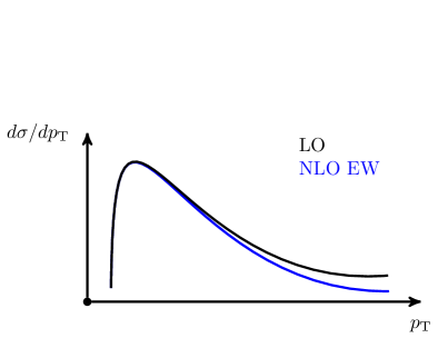
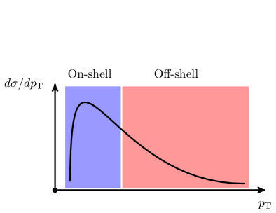
The two main aspects of this computation are the inclusion of EW corrections and of non-resonant contributions. Typically EW corrections become negatively large at high energy due to the effect of the so-called Sudakov logarithms. This is illustrated in a cartoon on the left-hand side of Fig. 1. In the same way, non-resonant contributions become sizeable in the tails of distributions. This is represented on the right-hand side of Fig. 1 where the on-shell region is dominated by the resonance while the off-shell region features sizeable non-resonant contributions. In both cases, these effects are critical in the high-energy tails of differential distributions which is the region where new physics is expected to appear. It is therefore crucial to have a good theoretical description of this part of phase space. With increasing experimental precision, this region will become accessible in the next few years, making such predictions indispensable.
This contribution is organised as follows: In the first part, results for the EW corrections are given. In the second section, the EW corrections are combined with the QCD ones using two different prescriptions.
2 Electroweak corrections
In this section we briefly present some differential distributions with EW corrections for at the LHC running at . For the details of the set-up we refer the reader to the original article [17].
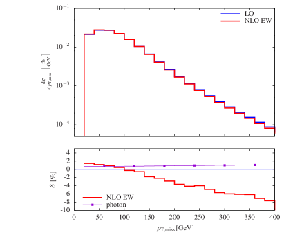
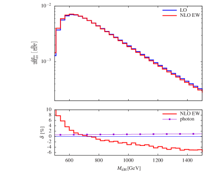
In Fig. 2 (left), the distribution in the missing transverse momentum is shown. The EW corrections display the typical Sudakov behaviour towards large transverse momentum. At GeV, the corrections reach about . For the invariant mass of the ttH system (right of Fig. 2), the corrections are positively large at threshold (above ). They decrease then steadily towards higher invariant mass and are at the level of around TeV.
3 Combination with QCD corrections
Let us now turn to the combination of the EW corrections with QCD corrections. Both NLO corrections are defined as
| (1) |
There exist multiple ways of combining them, but we focus here on two prescriptions. The first one is the so-called additive prescription which consists in adding both corrections
| (2) |
The second way of combining the two types of corrections is the multiplicative way. It is defined as:
| (3) |
Both prescriptions are equivalent at NLO accuracy. Nonetheless, the multiplicative one is usually preferred based on the argument of the factorisation of both types of corrections and consequently gives a better estimate of missing higher-order contributions of mixed type.
In the following, several cross sections and differential distributions are presented for at the LHC running at . Again, we refer the interested reader to Ref. [17] for details.
In Table 1, LO, NLO QCD, and NLO EW predictions are presented.***Note that and are not identical because different top widths have been used (see Ref. [17]). In addition, the numerical predictions for the combinations of the two NLO corrections are given. As can be seen, the difference between the two prescriptions is irrelevant. This is simply due to the fact that the NLO EW corrections are very small at the level of the total cross section.
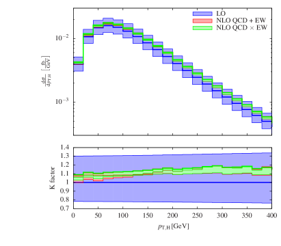
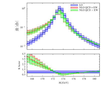
In Fig. 3, two differential distributions are shown for both the additive and the multiplicative combination of the NLO EW and QCD corrections. The plot on the left shows the transverse momentum of the Higgs boson. As for the total cross section, both prescriptions are very similar. This originates from the fact that the total corrections of this distribution are dominated by the QCD ones, while the EW corrections are small making the two combinations effectively identical. Turning to the differential distribution in the invariant mass of the reconstructed top quark (right), one can actually see differences between the two prescriptions. This is due to the large radiative tail for both types of corrections below the top-quark resonance, which leads to significant differences between the two combinations. These differences can give an estimate of missing higher-order corrections of mixed type.
4 Conclusion
In these proceedings results for the electroweak corrections to at the LHC have been presented. The main advantage of this computation is that it features EW corrections together with all off-shell and non-resonant effects. These corrections have been combined with the QCD ones following two prescriptions. All these effects will become particularly relevant in the next few years when the experimental precision will allow to explore further high-energy tails of differential distributions.
ACKNOWLEDGEMENTS
We are grateful to Robert Feger for providing and supporting the code MoCaNLO. The work of A.D. and M.P. was supported by the Bundesministerium für Bildung und Forschung (BMBF) under contract no. 05H15WWCA1. The research of M.P. has received funding from the European Research Council (ERC) under the European Union’s Horizon 2020 research and innovation programme (grant agreement No 683211).
References
- [1] W. Beenakker, S. Dittmaier, M. Krämer, B. Plümper, M. Spira and P. M. Zerwas, Phys. Rev. Lett. 87, 201805 (2001) [hep-ph/0107081].
- [2] W. Beenakker, S. Dittmaier, M. Krämer, B. Plümper, M. Spira and P. M. Zerwas, Nucl. Phys. B 653, 151 (2003) [hep-ph/0211352].
- [3] L. Reina and S. Dawson, Phys. Rev. Lett. 87, 201804 (2001) [hep-ph/0107101].
- [4] S. Dawson, C. Jackson, L. H. Orr, L. Reina and D. Wackeroth, Phys. Rev. D 68, 034022 (2003) doi:10.1103/PhysRevD.68.034022 [hep-ph/0305087].
- [5] S. Frixione, V. Hirschi, D. Pagani, H. S. Shao and M. Zaro, JHEP 1409, 065 (2014) [arXiv:1407.0823 [hep-ph]].
- [6] S. Frixione, V. Hirschi, D. Pagani, H.-S. Shao and M. Zaro, JHEP 1506, 184 (2015) [arXiv:1504.03446 [hep-ph]].
- [7] Y. Zhang, W. G. Ma, R. Y. Zhang, C. Chen and L. Guo, Phys. Lett. B 738, 1 (2014) [arXiv:1407.1110 [hep-ph]].
- [8] A. Kulesza, L. Motyka, T. Stebel and V. Theeuwes, JHEP 1603, 065 (2016) [arXiv:1509.02780 [hep-ph]].
- [9] A. Broggio, A. Ferroglia, B. D. Pecjak, A. Signer and L. L. Yang, JHEP 1603, 124 (2016) [arXiv:1510.01914 [hep-ph]].
- [10] A. Broggio, A. Ferroglia, B. D. Pecjak and L. L. Yang, JHEP 1702, 126 (2017) [arXiv:1611.00049 [hep-ph]].
- [11] A. Broggio, A. Ferroglia, R. Frederix, D. Pagani, B. D. Pecjak and I. Tsinikos, JHEP 1908, 039 (2019) [arXiv:1907.04343 [hep-ph]].
- [12] A. Kulesza, L. Motyka, D. Schwartländer, T. Stebel and V. Theeuwes, arXiv:2001.03031 [hep-ph].
- [13] R. Frederix, S. Frixione, V. Hirschi, F. Maltoni, R. Pittau and P. Torrielli, Phys. Lett. B 701, 427 (2011) [arXiv:1104.5613 [hep-ph]].
- [14] M. V. Garzelli, A. Kardos, C. G. Papadopoulos and Z. Trocsanyi, EPL 96, 11001 (2011) [arXiv:1108.0387 [hep-ph]].
- [15] H. B. Hartanto, B. Jager, L. Reina and D. Wackeroth, Phys. Rev. D 91, 094003 (2015) [arXiv:1501.04498 [hep-ph]].
- [16] A. Denner and R. Feger, JHEP 1511, 209 (2015) [arXiv:1506.07448 [hep-ph]].
- [17] A. Denner, J. N. Lang, M. Pellen and S. Uccirati, JHEP 1702, 053 (2017) [arXiv:1612.07138 [hep-ph]].
- [18] A. Manohar, P. Nason, G. P. Salam and G. Zanderighi, Phys. Rev. Lett. 117, 242002 (2016) [arXiv:1607.04266 [hep-ph]].
- [19] A. Denner and M. Pellen, JHEP 1608, 155 (2016) [arXiv:1607.05571 [hep-ph]].